Flow and Diffusion: Exact Solutions of Different Models Obtained with Traveling Wave and Self-Similar Transformations

Abstract

In this research work, we study different mathematical models that are capable of describing the particle diffusion phenomena in fluid flows. One-dimensional Cartesian models are defined to analyze the diffusion phenomena while they occur in a background stream. We derive exact solutions of the convection–diffusion equation with traveling wave and self-similar transformations in the case where the flow velocity is constant. The countable set of solutions presented is derived from the Gaussian distribution and from further solutions of the diffusion equation, which have even symmetry. In the case where the speed of the stream may vary, models for incompressible fluid flows are also considered. The investigated partial differential equation (PDE) systems are reduced to ordinary differential equation (ODE) systems with the self-similar Ansatz. The derived ODE systems for certain incompressible flows can be solved analytically, resulting in formulas containing Kummer’s M and Kummer’s U functions.

1. Introduction

Diffusion phenomena are important from a practical point of view and are among the most investigated transport processes in science (when particles are transported, we call it diffusion, and when energy is transported, we call it heat diffusion or heat conduction). The corresponding literature is enormous, so we just mention some fairly recent monographs [1,2,3,4]. A nice historical overview was written by Philibert [5]. Numerical methods for diffusion equations can be found in relevant studies [6,7,8,9].

Fluid flow—without any heat exchange—is another and even more relevant transport process with high complexity. The existing literature is considerable, so we just cite some textbooks [10,11,12,13]. To investigate the transport process in its full complexity, we need to couple diffusion and fluid flow problems [14,15,16,17]. There is a standard way to do this: considering the general form of conservation equations where the flow velocity is multiplied by the gradient of the concentration.

Shukha [18] published a state-of-the-art review of diffusion-induced hydrodynamic processes in 2001. He derived the conservation equations by making use of Onsager’s reciprocity relations, and basic solutions were presented for the binary and ternary fluid systems. These kinds of systems are also important from a biological point of view. As an example, we mention the diffusion and further transport dynamics of calcium in living cells, which was studied by Timofte [19].

In statistics, a similar description to the advection–diffusion equation is the Fokker–Planck equation. This equation is also characterized by diffusion and a possible drift term [20,21].

To broaden the horizon of our study, we should mention that as a far analogy, modern AI science also couples the phrases flow matching and diffusion [22,23]. In classical transport theory, diffusion in flow systems is described as the interplay between advection and stochastic spreading, typically formalized through the advection–diffusion equation. A velocity field transports material deterministically, while diffusion accounts for microscopic fluctuations that redistribute mass. Interestingly, modern generative models in artificial intelligence—particularly diffusion models and flow matching methods—rely on a mathematically analogous structure. In these models, probability density replaces physical density, and the evolution of a data distribution is governed by either a stochastic differential equation (diffusion models) or a velocity field (flow matching).

In a specific description for extended generality, according to the Benamou–Brenier dynamic formulation of optimal transport [24], the mass is transported between two distributions through a typically time-dependent velocity field that minimizes the kinetic energy.

Let us return to our physical systems. In recent years, we have investigated various Rayleigh–Bénard convection systems [25] and double-diffusion systems [26]—which are examples of the usual coupling—and presented analytical results. However, one may also consider other less well-known and less extensively studied diffusion-coupled flow phenomena in which the interaction between fluid flow and diffusion differs. All our presented models are based on certain phenomenological reasoning, which will be mentioned alongside the equations of the model and may eventually be derived from higher thermodynamic principles [27]. The aspects of irreversibility of the diffusion process have been discussed in Refs. [26,28].

In the following we present four models; all of them are formulated in one Cartesian space dimension. The first describes a diffusive flow with constant drift velocity, while the other three describe diffusion processes in incompressible fluid flows. We give physical interpretation of all our models. There are more generalizations possible, like the Darcy–Brinkman model, which describes diffusion in porous media [29,30], or reactive flows [31,32], which present certain situations for compressible or incompressible flows. The field of multiphase flow dynamics also discusses particle diffusion in fluid flows [33]. As a far-reaching aim, even magneto-hydrodynamical equations can be investigated [34] from the diffusion point of view.

As an investigation method, we apply the reduction mechanism with the self-similar Ansatz [35,36,37]. Our most important arguments in favor of this method are that it easily gives the Gaussian (or fundamental) solution of the regular diffusion equation and that the obtained self-similar exponents (in most cases) automatically show if a solution is convergent or divergent [38,39]. With this self-similar transformation, we have managed to solve diffusion systems, where we have found even and odd solutions of the diffusion equation beyond Gaussian solutions [38]. There are also cases where the diffusion coefficient is parameter-dependent [39,40,41]. Regarding two-dimensional systems, we have realized a comprehensive study of the two-dimensional heat diffusion equation, and the explicit self-similar Gaussian and non-Gaussian forms have been presented in [42]. In case of inhomogeneous media, two-dimensional diffusion has also been studied [43]. From a practical point of view, heat diffusion has also been analyzed in the context of insulation [44] or enhanced heat transfer [45]. In more complex cases or higher dimensions, numerical methods are also useful for such a class of systems [46]. Measurements with possible comparison to theoretical data support the importance of these phenomena and of different kinds of approaches [47,48]. The constant drift model can be solved with a quadrature that results in certain special analytic functions, while the coupled flow model needs a more complex evaluation method.

This paper presents solutions of the convection–diffusion equation which are beyond the Gaussian distribution, which travels in the sense of the stream. The first part of this study is an application of the results in diffusion found recently by the authors in research on the spreading phenomenon in streams. These solutions bring the possibility to describe diffusive phenomena for certain distributions of concentration which are not exactly the Gaussian distribution but are not far from it. Correspondingly this paper presents a countable set of advection non-Gaussian concentration profiles. The second part of this paper shows solutions of coupled equations of incompressible streams with diffusive material, where the streams may present decay in time.

2. The Models and the Derived Results

In general, diffusive flow has two aspects: one degree of freedom is related to flow and the other to diffusion. Usually, this means two functions, depending on the situation considered. To present a detailed analysis, we investigate the case of constant flow and another case, where the flow obeys the Navier–Stokes equation.

2.1. The Convection–Diffusion Equation

First, we discuss the spread of particles with concentration C which diffuse in an environment with velocity u. In this subsection, we consider this velocity to be constant and solve the problem relative to this constantly moving background. The model is intended to describe, among other things, the dispersion of pollutants in rivers or the local delivery of certain medications in blood vessels. The standard convection–diffusion equation is the following:

$${\displaystyle \frac{\partial C}{\partial t}}=-{\displaystyle \frac{\partial j}{\partial x}},$$

(1)

where j is the total current. The diffusion coefficient D is also considered constant in this model. The total current is composed of the diffusion current $-D{\displaystyle \frac{\partial C}{\partial x}}$ and the convective current $uC$

$$j=-D{\displaystyle \frac{\partial C}{\partial x}}+uC.$$

(2)

After evaluating the derivative on the right-hand side of Equation (1), one arrives at a standard form

$${\displaystyle \frac{\partial C}{\partial t}}=D{\displaystyle \frac{{\partial }^{2}C}{\partial x^2}}-u{\displaystyle \frac{\partial C}{\partial x}}.$$

(3)

At this point, we mention that this last equation is very similar to the Fokker–Planck equation, where instead of C there is a probability density function [20].

Equation (3) is homogeneous, which means that if $C(x,t)$ is a solution, then multiplying it by a constant also yields a solution of the problem. We treat the problem as a boundary value problem, which means that at the natural boundaries, plus and minus infinity, the concentration takes the same finite value. We solve the problem in the case where the boundary value is zero, with the observation that if $C(x,t)$ is solution of Equation (3), then $C_0+C(x,t)$ is also a solution, where $C_0$ is a constant. By this, the boundary value may differ from zero, depending on the background stream. One can choose this constant depending on further details of the problem.

In the first step, we make the transformation

$$\zeta =x-ut.$$

(4)

By this we arrive at a function $\tilde{C}(\zeta ,t)=C(x,t)$, which may still have an explicit dependence on t, beyond $\zeta$.

This change in variables characteristic of traveling wave problems yields the following:

$${\displaystyle \frac{\partial C}{\partial t}}={\displaystyle \frac{\partial \tilde{C}}{\partial t}}+{\displaystyle \frac{\partial \tilde{C}}{\partial \zeta }}{\displaystyle \frac{\partial \zeta }{\partial t}}={\displaystyle \frac{\partial \tilde{C}}{\partial t}}-u{\displaystyle \frac{\partial \tilde{C}}{\partial \zeta }}.$$

(5)

The other partial derivative with respect to x is

$${\displaystyle \frac{\partial C}{\partial x}}={\displaystyle \frac{\partial \tilde{C}}{\partial \zeta }}{\displaystyle \frac{\partial \zeta }{\partial x}}={\displaystyle \frac{\partial \tilde{C}}{\partial \zeta }},$$

(6)

with the second derivative

$${\displaystyle \frac{{\partial }^{2}C}{\partial x^2}}={\displaystyle \frac{{\partial }^2\tilde{C}}{\partial {\zeta }^2}},$$

(7)

This results in the following equation:

$${\displaystyle \frac{\partial \tilde{C}}{\partial t}}-u{\displaystyle \frac{\partial \tilde{C}}{\partial \zeta }}={\displaystyle \frac{{\partial }^2\tilde{C}}{\partial {\zeta }^2}}-u{\displaystyle \frac{\partial \tilde{C}}{\partial \zeta }}.$$

(8)

Finally, we arrive at the following equation of $\tilde{C}(\zeta ,t)$:

$${\displaystyle \frac{\partial \tilde{C}}{\partial t}}=D{\displaystyle \frac{{\partial }^2\tilde{C}}{\partial {\zeta }^2}}.$$

(9)

This equation is the diffusion equation in $\zeta$. The equation is important from many points of view, and a detailed analysis with a lot of practical solutions for finite horizons can be found in [4].

Equation (9) has quite a number of solutions for an infinite horizon, of which countable sets have certain symmetries, being even or odd [38]. At this point, we do not present the whole process which leads to the solutions, although for completeness we show some basic steps toward general solutions for extended domains. A self-similar transformation in the form $\tilde{C}(\zeta ,t)={\displaystyle \frac{1}{t^{\gamma }}}h\left(\eta \right)$, where $\eta =\zeta /\sqrt{t}$, transforms Equation (9) in the following way:

$$-\gamma h-{\displaystyle \frac{1}{2}}\eta {\displaystyle \frac{\partial h}{\partial \eta }}=D{\displaystyle \frac{{\partial }^{2}h}{\partial {\eta }^2}}.$$

(10)

In this equation, the parameter $\gamma$ remains free, and one arrives at a number of solutions depending on the parameter $\gamma$. The integer or half-integer values of this parameter lead to solutions which have odd or even symmetry.

2.1.1. The Fundamental Solution

The solutions of (9) have been widely discussed in classical works, from one to three dimensions [49]. This study covers the diffusion phenomena from a certain point of view, when the spreading takes place without boundary constraints.

We start with the fundamental solution of Equation (9), which is the Gaussian distribution regarding the variable $\zeta$,

$$\tilde{C}(\zeta ,t)=K_0{\displaystyle \frac{1}{\sqrt{t}}}{e}^{-{\displaystyle \frac{{\zeta }^2}{4Dt}}},$$

(11)

whose shape becomes wider as time goes by. $K_0$ is a constant that depends on the total amount which diffuses. If the total amount is a mass m, then this constant is considered to be $K_0=m/\sqrt{4D\pi }$. The solution has even symmetry in terms of $\zeta$. In this solution we insert $\zeta =x-ut$, and we get

$$C(x,t)={\displaystyle \frac{K_0}{\sqrt{t}}}{e}^{-{\displaystyle \frac{{(x-ut)}^2}{4Dt}}}={\displaystyle \frac{K_0}{\sqrt{t}}}{e}^{-{\displaystyle \frac{(x^2+u^2{t}^2-2xut)}{4Dt}}}.$$

(12)

In certain cases this solution is presented as follows:

$$C(x,t)={\displaystyle \frac{K_0}{\sqrt{t}}}{e}^{{\displaystyle \frac{u}{2D}}\left(x-{\displaystyle \frac{u}{2}}t\right)}{e}^{-{\displaystyle \frac{x^2}{4Dt}}}.$$

(13)

In this latter formula one can see that the Gaussian form which describes diffusion has a traveling amplitude.

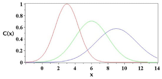
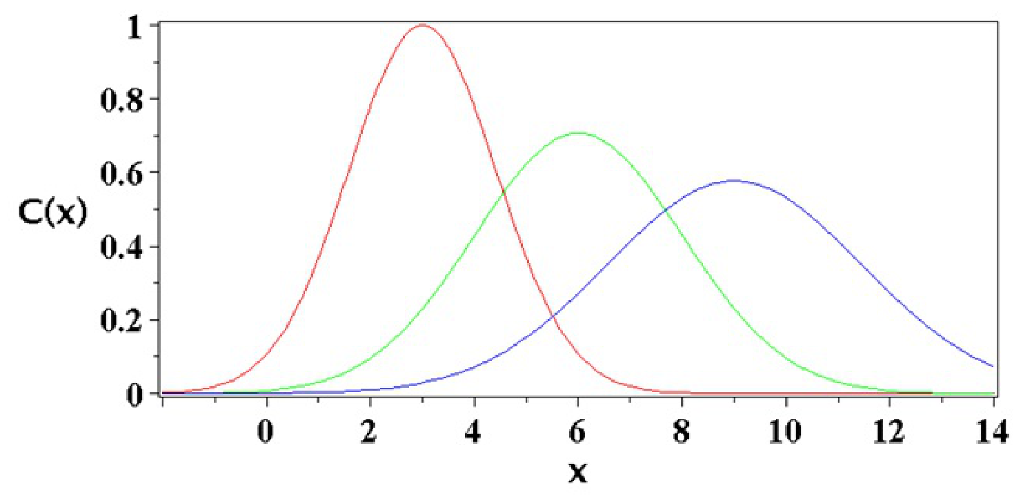
The form of this solution in presented in Figure 1. The figure shows the fundamental Gaussian form at different times. One can see that the shape of the Gaussian distribution becomes wider with time, and it drifts in the sense of the flow, while its maximum becomes lower. The above-mentioned equation is a solution for the initial condition $C(x,0)=\delta \left(x\right)$, and the convolution integral

$${\int }_{-\infty }^{\infty }{\displaystyle \frac{K_0}{\sqrt{t}}}{e}^{-{\displaystyle \frac{{(x-y-ut)}^2}{4Dt}}}\delta \left(y\right)dy={\displaystyle \frac{K_0}{\sqrt{t}}}{e}^{-{\displaystyle \frac{{(x-ut)}^2}{4Dt}}}.$$

results in Equation (12). This result can be interpreted as a distribution in the case where a locally introduced material spreads out in the presence of a flow.

Figure 1. The shape of the function in (13) for different times. In this figure, $K_0=1,D=1$, and $u=3$. The red, green, and blue lines correspond to the times $t=1,2,3$.

2.1.2. Further Quasi-Symmetric Solutions Related to Even Solutions of Diffusion Equation

Searching for further solutions of (9) beyond the fundamental one is a difficult task, and different schools have approached the problem. An interesting study is that by Bluman and Cole [50]: they arrived at slightly more general arguments than the ones presented above, with methods of Lie algebra.

An important breakthrough was realized in [38,51], where self-similar and algebraic methods were combined to arrive at further solutions.

Equation (10) has as solution the following shape function for $\gamma =3/2$:

$$h\left(\eta \right)=e^{-{\displaystyle \frac{{\eta }^2}{4D}}}\left(1-{\displaystyle \frac{{\eta }^2}{2D}}\right).$$

(14)

The index $n=2\gamma -1=2$ can be associated with this solution considering that the binomial term beside the Gaussian distribution can be adjusted to be proportional to the second-degree Hermite polynomial.

By this we arrive at the next even solution in terms of $\zeta$ of Equation (9):

$$\tilde{C}(\zeta ,t)=K_1{\displaystyle \frac{1}{\sqrt{t^3}}}{e}^{-{\displaystyle \frac{{\zeta }^2}{4Dt}}}\left(1-{\displaystyle \frac{{\zeta }^2}{2Dt}}\right),$$

(15)

where $K_1$ is a constant. The solution is symmetric relative to the parameter $\zeta$, which is the coordinate in the co-moving frame of the stream. This solution can be considered, in a certain sense, to be the first even possible adjustment to the Gaussian distribution. Correspondingly, the concentration C as a function of x and t is

$$C(x,t)=K_1{\displaystyle \frac{1}{\sqrt{t^3}}}{e}^{-{\displaystyle \frac{{(x-ut)}^2}{4Dt}}}\left(1-{\displaystyle \frac{{(x-ut)}^2}{2Dt}}\right).$$

(16)

The shift in the maximum in time and the decay of the amplitude can be better seen in the following form:

$$C(x,t)=K_1{\displaystyle \frac{1}{\sqrt{t^3}}}{e}^{{\displaystyle \frac{u}{2D}}\left(x-{\displaystyle \frac{u}{2}}t\right)}{e}^{-{\displaystyle \frac{x^2}{4Dt}}}\left(1-{\displaystyle \frac{{(x-ut)}^2}{2Dt}}\right).$$

(17)

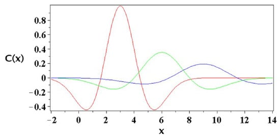
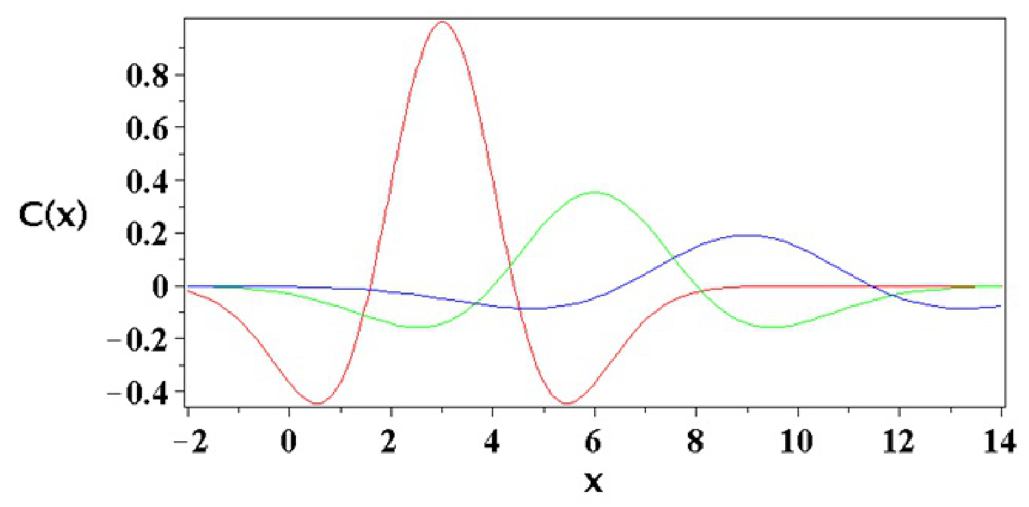
This solution is presented in Figure 2.

Figure 2. The function $C(x,t)$ of Equation (17) for different times. In this figure, $K_1=1,D=1$, and $u=3$. The red, green, and blue lines correspond to the times $t=1,2,3$.

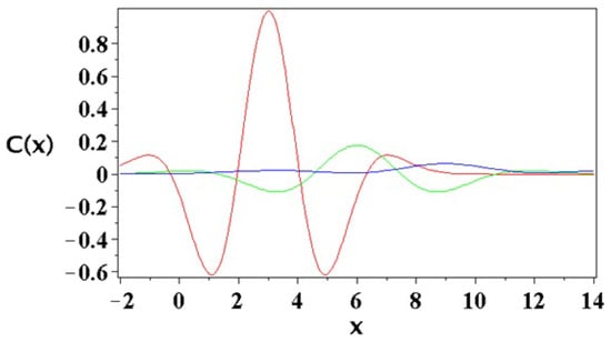
It is interesting to see that Figure 2 shows functions which have fine details and may go below the zero value. The concentration presented should be considered an additional concentration to a background value of C, or to the Gaussian distribution presented above.

The next even-shape function, which can be derived from (10), for $\gamma =5/2$ is

$$h\left(\eta \right)=e^{-{\displaystyle \frac{{\eta }^2}{4D}}}\left(1-{\displaystyle \frac{{\eta }^2}{D}}+{\displaystyle \frac{{\eta }^4}{12D}}\right).$$

(18)

The polynomial form beside the Gaussian distribution corresponds to the fourth-order Hermite polynomial, with index $n=4$. As a consequence, Equation (9) has the solution for infinite horizon, related to exponential and polynomial forms:

$$\tilde{C}(\zeta ,t)=K_2{\displaystyle \frac{1}{\sqrt{t^5}}}{e}^{-{\displaystyle \frac{{\zeta }^2}{4Dt}}}\left(1-{\displaystyle \frac{{\zeta }^2}{Dt}}+{\displaystyle \frac{{\zeta }^4}{12D^2{t}^2}}\right),$$

(19)

where $K_2$ is a constant.

The corresponding solution in terms of x and t is given by the following relation:

$$C(x,t)=K_2{\displaystyle \frac{1}{\sqrt{t^5}}}{e}^{-{\displaystyle \frac{{(x-ut)}^2}{4Dt}}}\left(1-{\displaystyle \frac{{(x-ut)}^2}{Dt}}+{\displaystyle \frac{{(x-ut)}^4}{12D^2{t}^2}}\right).$$

(20)

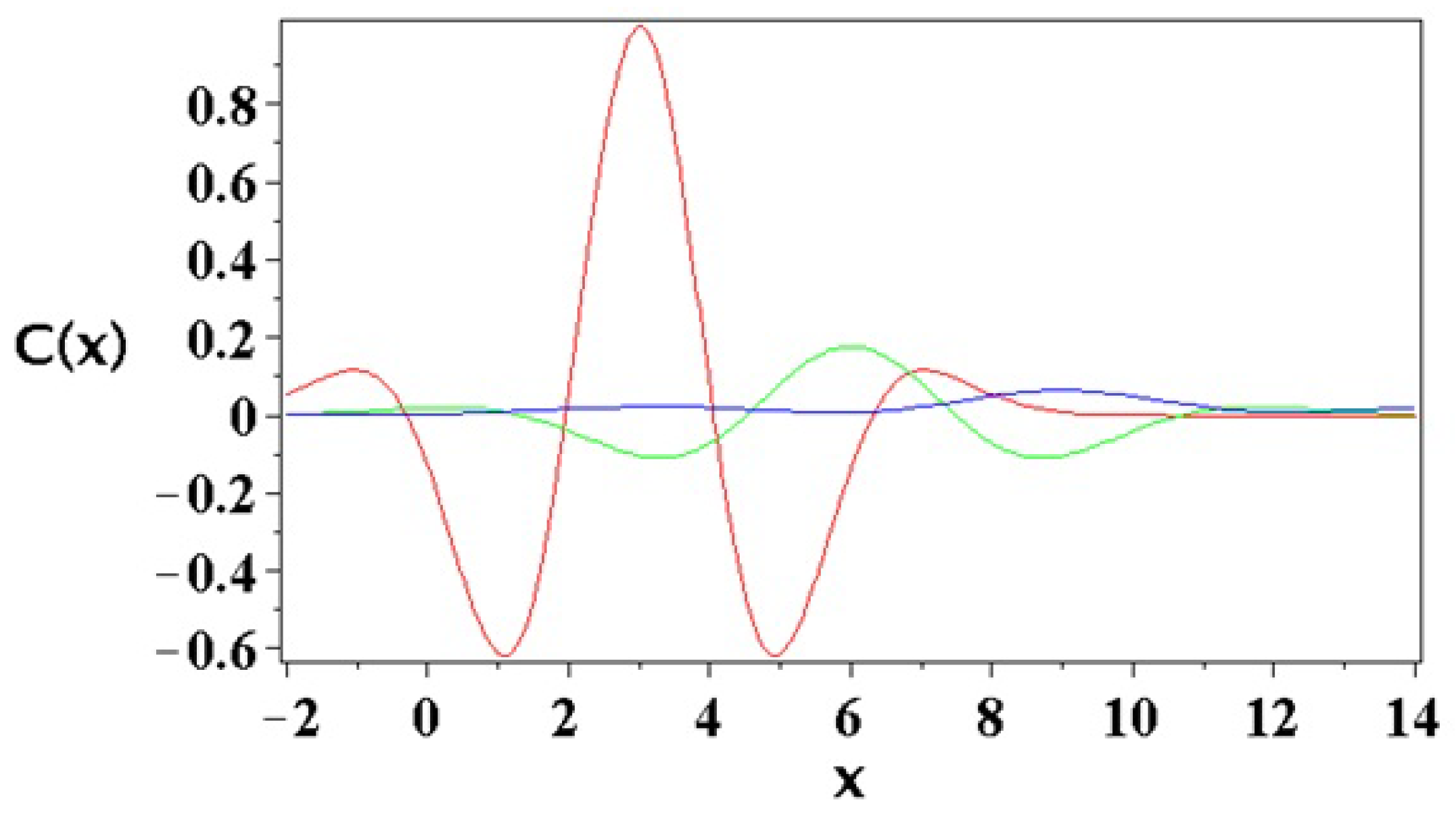
One can see this solution for different times in Figure 3. This third solution has even more oscillations and can express possible additional details of particle distributions relative to the normal distribution.

Figure 3. The function $C(x,t)$ of Equation (20) for different times. In this figure, $K_2=1,D=1$, and $u=3$. The red, green, and blue lines correspond to the times $t=1,2,3$.

These functions show further possibilities as solutions of the diffusion–convection equation. In practice, one can rather conceive linear combinations of these solutions which may appear beside the Gaussian distribution. By this, one may arrive at more diversified possibilities of analytical description of diffusion in streams.

We also mention the following solution for $\gamma =7/2$:

$$\begin{array}{ccc}\hfill C(x,t)& =& K_3{\displaystyle \frac{1}{t^{\frac{7}{2}}}}{e}^{-{\displaystyle \frac{{(x-ut)}^2}{4Dt}}}(1-{\displaystyle \frac{3}{2Dt}}{(x-ut)}^2\hfill \\ & +& {\displaystyle \frac{1}{4D^2{t}^2}}{(x-ut)}^4-{\displaystyle \frac{1}{120D^3{t}^3}}{(x-ut)}^6),\hfill \end{array}$$

(21)

where $K_3$ is a constant. Further properties of the solutions presented above can be found in Appendix A. To assure the positivity of the concentration, the solutions beyond the Gaussian one can be considered perturbations or adjustments to a constant concentration or to the Gaussian distribution so that the total concentration remains positive.

In the following, we consider the possibility of certain flows that are not constant in space or time. In principle, for non-constant flows, there are two special cases: one, the flow does not depend on the space variable but depends on time; the other, it conversely depends on space and not time. Even though the setup seems to allow for more kinds of dependencies, the incompressible principle with the diffusion equation will constrain the variation in fluid flow velocity.

2.2. Incompressible Models with Non-Constant Stream

We start with the usual description in one Cartesian space dimension where the continuity, Navier–Stokes and diffusion equations are coupled together:

$$\begin{array}{ccc}\hfill u_x& =& 0,\hfill \end{array}$$

(22)

$$\begin{array}{ccc}\hfill u_t+u{u}_x& =& -{\displaystyle \frac{p_x}{\rho }}+\nu u_{xx},\hfill \end{array}$$

(23)

$$\begin{array}{ccc}\hfill C_t+u{C}_x& =& D{C}_{xx}.\hfill \end{array}$$

(24)

From now on subscripts mean partial derivatives in respect to time and space throughout the whole study. The three dynamical variables are velocity $u(x,t)$, pressure $p(x,t)$ and concentration $C(x,t)$, and the three additional parameters of the physical constant are fluid density $\rho$, fluid viscosity $\nu$, and regular diffusion coefficient D. For stability reasons, D should be a positive real number. The same notation will be used in all three models. Due to the conservation of mass, momenta and particle number, this is the usual coupling of diffusion to fluid flows. The importance of the term $u{C}_x$ is well described in ref. [52]. All the left-hand sides of the equations describe the conservation of physical quantities with the help of the substantial derivative. The temporal change in the physical quantity is proportional to the flux and the quantity which flows in or out of the volume, plus the existing sources or minus the existing sinks, which are usually written on the right-hand side of the equations and describe mass variation.

In principle there are a number of possibilities for solving the presented system, and in the following, we will consider certain cases. Because of the one-dimensional incompressibility criterion $u_x=0$, $u_{xx}$ also vanishes, and the following specific self-similar transformation yields a variation in u in time rather than in space.

As a second model we may consider that diffusion is just coupled to the flow rather than to a source term. So the medium which undergoes diffusion has a source or sink:

$$\begin{array}{ccc}\hfill u_x& =& 0,\hfill \end{array}$$

(25)

$$\begin{array}{ccc}\hfill u_t+u{u}_x& =& -{\displaystyle \frac{p_x}{\rho }}+\nu u_{xx},\hfill \end{array}$$

(26)

$$\begin{array}{ccc}\hfill C_t& =& D{C}_{xx}+au,\hfill \end{array}$$

(27)

where a is the strength of the source term with the proper physical dimension. This model can be interpreted as a system, where the concentration C may have a source; i.e., a river has a concentration of a certain material, and the flow may dissolve this material from the bottom or bank of the river. In this model, the dissolution of material from the riverbed is proportional to the flow speed. This may typically happen if the bottom is a salty or calcareous environment. Regarding sources which come from reaction, one can find further details in Ref. [53].

We consider the viscosity constant; however, in certain cases of non-Newtonian fluids, viscosity is a power-law function of fluid velocity [54].

We seek the solutions of these flow systems in the following self-similar form Refs. [36,37]:

$$\begin{array}{ccc}\hfill u(x,t)& =& t^{-\alpha }·f\left({\displaystyle \frac{x}{t^{\beta }}}\right)=t^{-\alpha }f\left(\eta \right),\hfill \end{array}$$

(28)

$$\begin{array}{ccc}\hfill p(x,t)& =& t^{-\delta }·g\left(\eta \right),\hfill \end{array}$$

(29)

$$\begin{array}{ccc}\hfill C(x,t)& =& t^{-\gamma }·h\left(\eta \right).\hfill \end{array}$$

(30)

where $f\left(\eta \right),g\left(\eta \right)$ and $h\left(\eta \right)$ are the three independent shape functions depending on the reduced variable $\eta$ with the needed existing first and second continuous derivatives. Additionally, $\alpha ,\beta ,\gamma$ and $\delta$ are all real numbers and are called self-similar exponents. Usually, positive $\alpha ,\delta$ and $\gamma$ exponents mean a solution which decays as time goes to infinity. Negative exponents mean diverging solutions in general. Positive $\beta$ dictates the spreading of the solutions in time. We continue with the detailed analysis of all these three models. The time derivative of u can be written as follows:

$$u_t=-\alpha t^{-\alpha -1}f-\beta t^{-\alpha -1}\eta f^{\prime },$$

(31)

Above and in the following, primes ^′ denote derivation with respect to $\eta$. The derivative in time of C is similar and can be found if $\alpha$ is replaced with $\gamma$. The first derivative in the spatial variable is

$$u_x=t^{-\alpha }{f}^{\prime }{\displaystyle \frac{\partial \eta }{\partial x}}=t^{-\alpha -\beta }{f}^{\prime }.$$

(32)

The first spatial derivatives of p and C can be evaluated correspondingly with the exponents $\delta$ and $\gamma$. The second derivative in x is

$$u_{xx}=t^{-\alpha -\beta }{f}^{″}{\displaystyle \frac{\partial \eta }{\partial x}}=t^{-\alpha -2\beta }{f}^{″}.$$

(33)

From the first system, Equations (22)–(24), after some algebraic steps, we can easily derive the coupled ODE system for the shape functions with the self-similar exponents as constraints conditions. After simplifications, the ODE system reads as follows:

$$\begin{array}{ccc}\hfill f^{\prime }& =& 0,\hfill \end{array}$$

(34)

$$\begin{array}{ccc}\hfill -{\displaystyle \frac{f}{2}}-{\displaystyle \frac{\eta f^{\prime }}{2}}+f{f}^{\prime }& =& -{\displaystyle \frac{g^{\prime }}{\rho }}+\nu f^{″},\hfill \end{array}$$

(35)

$$\begin{array}{ccc}\hfill -\gamma h-{\displaystyle \frac{h^{\prime }\eta }{2}}+f{h}^{\prime }& =& D{h}^{″}.\hfill \end{array}$$

(36)

The exact values of the self-similar exponents are $\alpha =\beta ={\displaystyle \frac{1}{2}}$ and $\delta =1$, and $\gamma$ remains an arbitrary real number. For these values of the exponents, the LHS and RHS of the above Equations (22)–(24) have the same temporal decay. The solutions can be determined by integration:

$$\begin{array}{ccc}\hfill f\left(\eta \right)& =& c_1,u(x,t)={\displaystyle \frac{c_1}{t^{\frac{1}{2}}}},\hfill \end{array}$$

(37)

$$\begin{array}{ccc}\hfill g\left(\eta \right)& =& {\displaystyle \frac{c_1\rho \eta }{2}}+c_2,p(x,t)={\displaystyle \frac{c_1\rho x/t^{\frac{1}{2}}+c_2}{t}},\hfill \end{array}$$

(38)

$$\begin{array}{ccc}\hfill h\left(\eta \right)& =& c_3\mathrm{M}\left(\gamma ,{\displaystyle \frac{1}{2}},-{\displaystyle \frac{{(2c_1-\eta )}^2}{4D}}\right)+c_4\mathrm{U}\left(\gamma ,{\displaystyle \frac{1}{2}},-{\displaystyle \frac{{(2c_1-\eta )}^2}{4D}}\right),\hfill \end{array}$$

(39)

$$\begin{array}{ccc}\hfill C(x,t)& =& t^{-\gamma }·\left(c_3\mathrm{M}\left[\gamma ,{\displaystyle \frac{1}{2}},-{\displaystyle \frac{{(2c_1-[x/t^{\frac{1}{2}}])}^2}{4D}}\right]+c_4\mathrm{U}\left[\gamma ,{\displaystyle \frac{1}{2}},-{\displaystyle \frac{{(2c_1-[x/t^{\frac{1}{2}}])}^2}{4D}}\right]\right),\hfill \end{array}$$

(40)

From now on, all $c_i$ parameters are considered real integration constants. The velocity and the pressure fields are relatively simple. By this, the topic of the section becomes a study of time-varying advection. The concentration is more complex and depends on Kummer’s M and Kummer’s U functions [55,56]. The validity of the solution in (39) is proven in Appendix B. Note that now there are no extra Gaussian weight functions present.

Because the argument of Kummer’s functions $z=-{\displaystyle \frac{{(2c_1-\eta )}^2}{4D}}$ is always negative or zero, the asymptotic behavior of these functions is given by the value of the parameter $\gamma$ [55]. In general we have the expectation that negative $\gamma$ parameters give rather divergent solutions and positive $\gamma$ parameters mean decaying solutions.

Regarding regularity of the U function, we have the following observation: The asymptotic behavior of U for large values of $\left|z\right|$ is $\mathrm{U}(\gamma ,1/2,-|z\left|\right)\sim {\left|z\right|}^{-\gamma }{e}^{-i\pi \gamma }$, which is a decaying function for positive $\gamma$; for these values, the function remains finite.

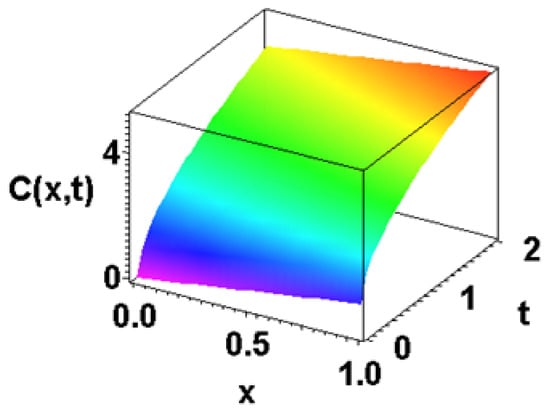
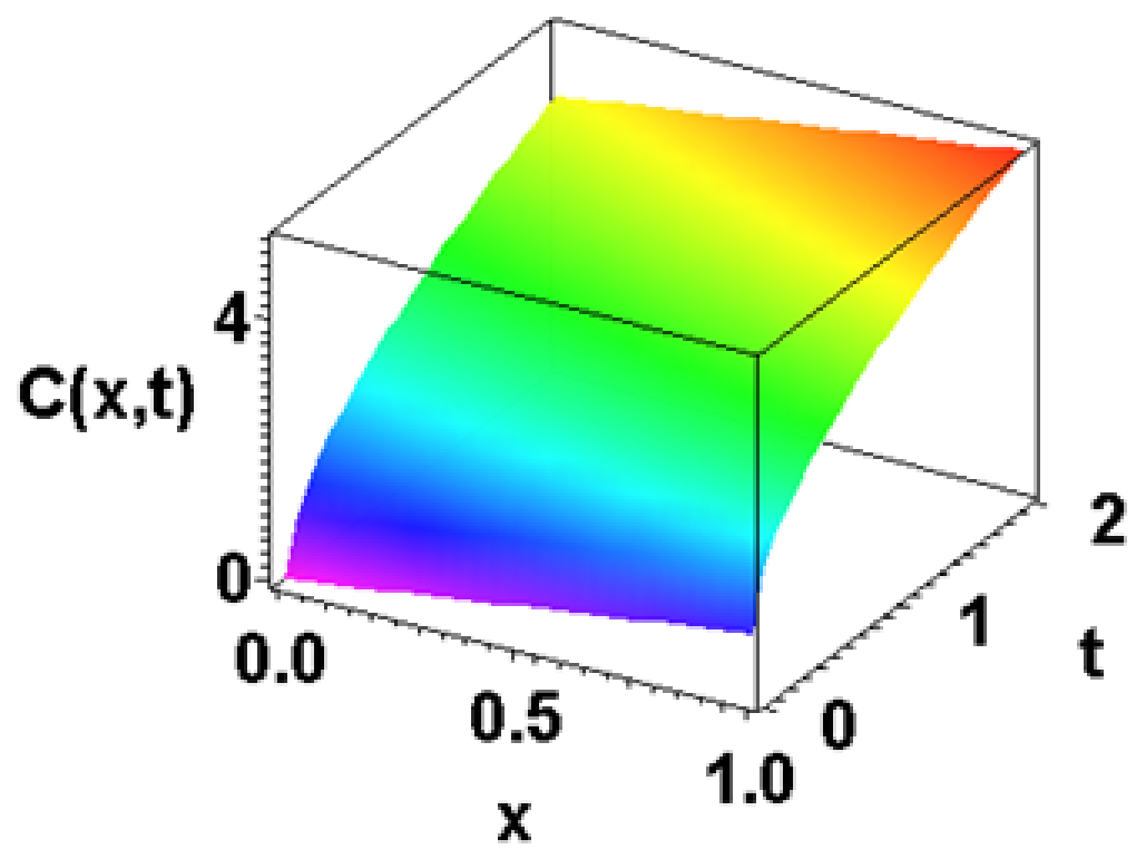
The solution of the diffusion equation in this case only shows a difference relative to the first model. Therefore, we focus on analyzing its properties. For understanding the main features of the solutions, one can see that the shape functions is also composed from special Kummer’s function and, from this point of view, may have certain similar properties. In an interesting way, in the latter model, there is no explicit decay in terms of exponential function. Figure 4 shows Equation (40) for the parameters of $\gamma =1/2,c_1=1/2,c_3=1,c_4=0$ and $D=1$. In this case Kummer’s M function gives a regular behavior at the boundaries as well.

Figure 4. The figure shows Equation (40) for the values $\gamma =1/2,c_1=1/2$ and $c_4=0$. All the other previously not specified parameters are set to unity.

Regarding integrability of Kummer’s functions, it depends on the parameter $\gamma$. The most straightforward case is $c_3\ne 0$ and $c_4=0$. In this case the integrability of Kummer’s M function can support the physical feature of the concentration. If $\gamma =0$, for $c_1=1$ and $D=1$, one has

$$\mathrm{M}\left(0,{\displaystyle \frac{1}{2}},-{\displaystyle \frac{{(2-\eta )}^2}{4}}\right)=1.$$

(41)

If one integrates it, the integral is divergent.

For $\gamma =1/2$, we have the following integral:

$${\int }_{-\infty }^{\infty }\mathrm{M}\left({\displaystyle \frac{1}{2}},{\displaystyle \frac{1}{2}},-{\displaystyle \frac{{(2-\eta )}^2}{4}}\right)d\eta =2\sqrt{\pi }.$$

(42)

This means that this integral is finite and that the integrand can be related to a possible physical solution of the equation system with finite mass.

For a higher value $\gamma =3/2$, the integral is also finite:

$${\int }_{-\infty }^{\infty }\mathrm{M}\left({\displaystyle \frac{3}{2}},{\displaystyle \frac{1}{2}},-{\displaystyle \frac{{(2-\eta )}^2}{4}}\right)d\eta =0.$$

(43)

Similarly, the integral for $\gamma =5/2$ yields

$${\int }_{-\infty }^{\infty }\mathrm{M}\left({\displaystyle \frac{5}{2}},{\displaystyle \frac{1}{2}},-{\displaystyle \frac{{(2-\eta )}^2}{4}}\right)d\eta =0.$$

(44)

One can see that there are solutions of the presented model which have finite integrals. The concentrations related to these solutions belong to a finite-mass system.

The second model, Equations (25)–(27), has internal self-similar symmetry with all fixed exponents $\alpha =1/2,\beta =1/2,\delta =1,\gamma =-1/2$, which assure, for the RHS and LHS of the governing equations, the same temporal decay as one can see in Appendix C. The following ODE system is obtained:

$$\begin{array}{ccc}\hfill f^{\prime }& =& 0,\hfill \end{array}$$

(45)

$$\begin{array}{ccc}\hfill -{\displaystyle \frac{f}{2}}-{\displaystyle \frac{\eta f^{\prime }}{2}}+f{f}^{\prime }& =& -{\displaystyle \frac{g^{\prime }}{\rho }}+\nu f^{″},\hfill \end{array}$$

(46)

$$\begin{array}{ccc}\hfill +{\displaystyle \frac{h}{2}}-{\displaystyle \frac{h^{\prime }\eta }{2}}& =& D{h}^{″}+af.\hfill \end{array}$$

(47)

One can see that Equation (47) has an interesting symmetry. The equation remains unchanged under the change in the variables $\eta \to -\eta$ and $h(-\eta )\to h\left(\eta \right)$, which means that we can expect at least an even-symmetry solution.

The velocity and the pressure fields are the same as Equations (37) and (38). Due to the fixed negative value of the $\gamma$ self-similar exponent, the shape function $h\left(\eta \right)$ and the concentration distribution $C(x,t)$ have the form

$$\begin{array}{ccc}\hfill h\left(\eta \right)& =& \left(D{e}^{-{\displaystyle \frac{{\eta }^2}{4D}}}+{\displaystyle \frac{\sqrt{D\pi }}{2}}·\eta ·\mathrm{erf}\left[{\displaystyle \frac{\eta }{2\sqrt{D}}}\right]\right)c3+\eta c_4+2a{c}_1,\hfill \end{array}$$

(48)

$$\begin{array}{ccc}\hfill C(x,t)& =& t^{{\displaystyle \frac{1}{2}}}·\left(\left[D{e}^{-{\displaystyle \frac{x^2}{4Dt}}}+{\displaystyle \frac{\sqrt{D\pi }x}{2\sqrt{t}}}·\mathrm{erf}\left\{{\displaystyle \frac{x}{2\sqrt{Dt}}}\right\}\right]c3+c_4{\displaystyle \frac{x}{\sqrt{t}}}+2a{c}_1\right),\hfill \end{array}$$

(49)

where erf$\left\{\right\}$ is the Gauss error function [55,56]. Due to the negative exponent $\gamma$, the concentration $C(x,t)$ has a slight divergence in time, which can be explained by the presence of the source. Beyond the mathematical result, from a physical point of view, these equations are valid for the time in which one can afford the source supply of Equation (27).

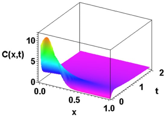
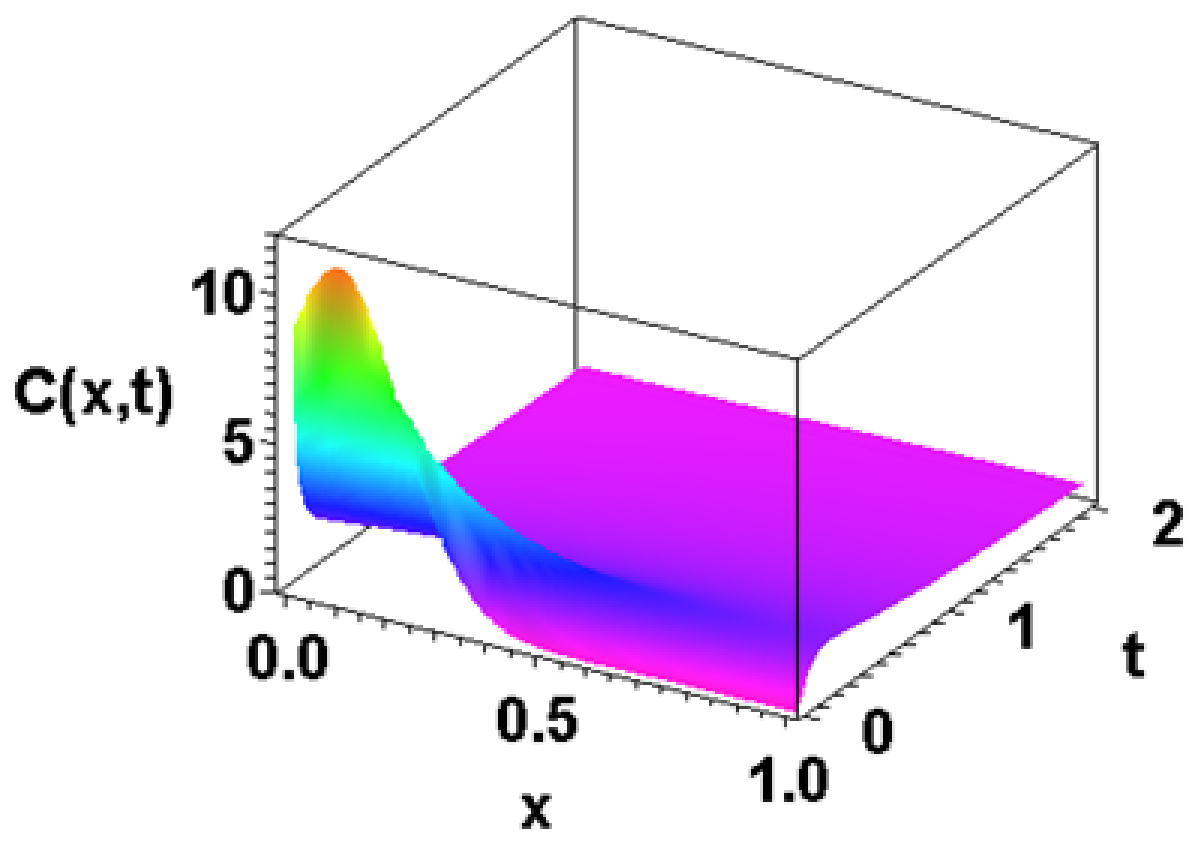
Figure 5 shows Equation (49) for $\gamma =-1/2$ with all other parameters set to unity. The function exhibits a square-root increase in time, which is due to the presence of the source in the dynamics. In an interesting way, this increase is less than linear, because the source itself, as result of the solution of the system, has a slight decrease in time.

Figure 5. The function $C(x,t)$ of Equation (49) for $\gamma =-{\displaystyle \frac{1}{2}}$. The diffusion coefficient $D=1$, while the other constants $a=1$, $c_1=1$, $c_3=1$ and $c_4=1$.

We also present the case, as a third incompressible model, where both the stream and the source term are present.

$$\begin{array}{ccc}\hfill u_x& =& 0,\hfill \end{array}$$

(50)

$$\begin{array}{ccc}\hfill u_t+u{u}_x& =& -{\displaystyle \frac{p_x}{\rho }}+\nu u_{xx},\hfill \end{array}$$

(51)

$$\begin{array}{ccc}\hfill C_t+u{C}_x& =& D{C}_{xx}+au.\hfill \end{array}$$

(52)

This system with convection and source can be transformed, using the self-similar Ansatz, and one arrives at the following system of equations. The complexity comes from the fact that it has the constraints which come from convection and from the presence of the source.

We use the self-similar transformation presented in (28)–(30). The exponents are all fixed in this construction as $\alpha =1/2,\beta =1/2,\delta =1,\gamma =-1/2$, resulting in the ODE system

$$\begin{array}{ccc}\hfill f^{\prime }& =& 0,\hfill \end{array}$$

(53)

$$\begin{array}{ccc}\hfill -{\displaystyle \frac{f}{2}}-{\displaystyle \frac{\eta f^{\prime }}{2}}+f{f}^{\prime }& =& -{\displaystyle \frac{g^{\prime }}{\rho }}+\nu f^{″},\hfill \end{array}$$

(54)

$$\begin{array}{ccc}\hfill +{\displaystyle \frac{h}{2}}-{\displaystyle \frac{h^{\prime }\eta }{2}}+f{h}^{\prime }& =& D{h}^{″}+af.\hfill \end{array}$$

(55)

The solution of this system is $f=c_1$, which is constant. The next shape function $g=c_1\rho {\displaystyle \frac{\eta }{2}}$ if there is no free term, and the corresponding form of pressure is $p={\displaystyle \frac{1}{t}}{c}_1\rho {\displaystyle \frac{x}{2\sqrt{t}}}$, which shows the evolution of this quantity.

The expression of h is the following:

$$h\left(\eta \right)=C_2(-2c_1+\eta )+C_1\left(2\sqrt{\pi D}{e}^{{\displaystyle \frac{\eta (4c_1-\eta )}{D}}}+(2c_1-\eta )e^{{\displaystyle \frac{c{1}^2}{D}}}·erf\left({\displaystyle \frac{c_1-\frac{\eta }{2}}{\sqrt{D}}}\right)\pi \right)+2a{c}_1,$$

(56)

which is specific for dynamics.

The corresponding C(x,t) is

$$\begin{array}{ccc}\hfill C(x,t)& =& t^{{\displaystyle \frac{1}{2}}}[C_2\left({\displaystyle \frac{x}{\sqrt{t}}}-2c_1\right)+2a{c}_1\hfill \\ & +& C_1(2\sqrt{\pi D}{e}^{{\displaystyle \frac{\frac{x}{\sqrt{t}}(4c_1-\frac{x}{\sqrt{t}})}{D}}}+\left(2c_1-{\displaystyle \frac{x}{\sqrt{t}}}\right)e^{{\displaystyle \frac{c{1}^2}{D}}}·erf\left({\displaystyle \frac{c_1-\frac{x}{2\sqrt{t}}}{\sqrt{D}}}\right)\pi )].\hfill \end{array}$$

(57)

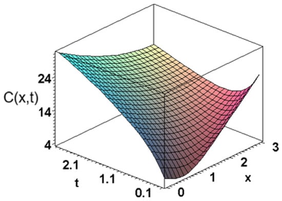
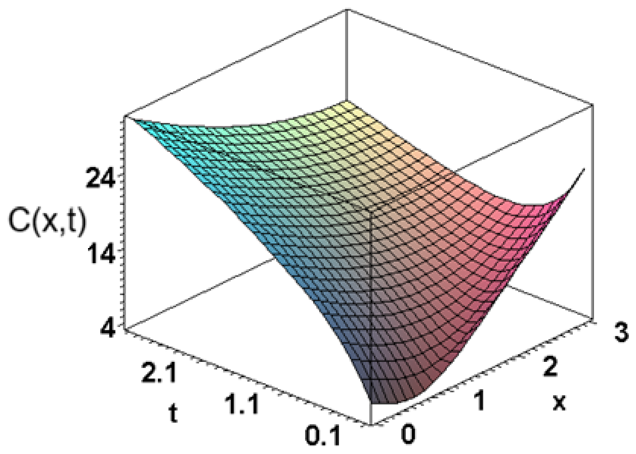
This function is presented in Figure 6.

Figure 6. The function $C(x,t)$ of Equation (57) for $\gamma =-{\displaystyle \frac{1}{2}}$. The diffusion coefficient $D=1$, and $c_1=1,C_2=1,C_1=1,a=1$.

One can see that this last solution has a specific shape. The shape of the function shows the variety characterized by both source and the flow in the system.

3. Summary and Outlook

In the presented study, we investigated four different types of coupling mechanisms between viscous fluid flow and diffusion phenomena. Incompressible one-dimensional systems were investigated with the self-similar Ansatz. For these systems, most of the results are analytical and can be expressed with Kummer’s M and Kummer’s U functions or with the error functions. In case of constant flow velocity, the results show a part which expresses the presence of the stream and another part which shows diffusion. Regarding the diffusive part, the presented functions have even symmetry: one of them is the Gaussian, and the others are further even solutions of the diffusion equation found recently by the authors.

In the other cases, where the stream may vary in time, the stream still remains incompressible, and the results depend on further details of the dynamics. If there is no source term in the dynamics, the results can be expressed in terms of Kummer functions, which have reasonable decay, a characteristic of diffusive phenomena. In the presence of particle source in dynamics, the solution is still analytic in terms of the error function and has a temporal increase because of the mass inflow due to the source.

Further works are in progress to find and analyze models that are capable of describing more complex diffusion phenomena like reactive flows [31] that combine elements of our first and third models.

A second kind of straightforward option is to investigate the same systems in a spherical coordinate system; due to the additional $1/r$ factors, singular solutions may emerge.

References

- Cussler, E.L. Diffusion: Mass Transfer in Fluid Systems, 3rd ed.; Cambridge University Press: Cambridge, UK, 2009. [Google Scholar]
- Ghez, R. Diffusion Phenomena; Dover Publications Inc.: Mineola, NY, USA, 2018. [Google Scholar]
- Bunde, A.; Caro, J.; Kärger, J.; Vogl, G. Diffusive Spreading in Nature, Technology and Society; Springer: Berlin/Heidelberg, Germany, 2018. [Google Scholar]
- Thambynayagam, R.K.M. The Diffusion Handbook: Applied Solutions for Engineers; McGraw-Hill: New York, NY, USA, 2011. [Google Scholar]
- Philibert, J. One and a half century of diffusion: Fick, Einstein, before and beyond. Diffus. Fundam. 2005, 2, 1.1–1.10. [Google Scholar] [CrossRef] [Scilit]
- Holmes, M.H. Introduction to Numerical Methods in Differential Equations; Springer: New York, NY, USA, 2007. [Google Scholar]
- Versteeg, H.K.; Malalasekera, W. An Introduction to Computational Fluid Dynamics, 2nd ed.; Pearson Education Limited: Harlow, UK, 2007. [Google Scholar]
- Jalghaf, H.K.; Kovács, E.; Majár, J.; Nagy, A.; Askar, A.H. Explicit Stable Finite Difference Methods for Diffusion-Reaction Type Equations. Mathematics 2021, 9, 3308. [Google Scholar] [CrossRef] [Scilit]
- Kovács, E.; Majár, J.; Saleh, M. Unconditionally Positive, Explicit, Fourth Order Method for the Diffusion- and Nagumo-Type Diffusion-Reaction Equations. J. Sci. Comput. 2024, 98, 39. [Google Scholar] [CrossRef] [Scilit]
- Batchelor, G. An Introduction to Fluid Dynamics; Cambridge University Press: Cambridge, UK, 1967. [Google Scholar]
- Landau, L.D.; Lifshitz, E. Fluid Mechanics, 2nd ed.; Pergamon Press: Oxford, UK; Elmsford, NY, USA, 1987. [Google Scholar]
- Eckert, M. The Dawn of Fluid Mechanics: A Discipline Between Science and Technology; Wiley-VCH, Verlag GmBH & Co.KgaA: Weinheim, Germany, 2006. [Google Scholar]
- Nazarenko, S. Fluid Dynamics via Examples and Solutions; CRC Press (Taylor Francis Group): Boca Raton, FL, USA, 2014. [Google Scholar]
- Bennett, T.D. Transport by Advection and Diffusion: Momentum, Heat and Mass Transfer; John Wiley & Sons: Hoboken, NJ, USA, 2013. [Google Scholar]
- Newman, J.; Battaglia, V. The Newman Lectures on Transport Phenomena; Jenny Stanford Publishing: Singapore, 2021. [Google Scholar]
- Ashan, A. Convection and Conduction Heat Transfer; IntechOpen: Rijeka, Croatia, 2011. [Google Scholar]
- Klages, R. Microscopic Chaos, Fractals and Transport in Nonequilibrium Statistical Mechanics; Advanced Series in Nonlinear Dynamics; World Scientific: Singapore, 2007; Volume 24. [Google Scholar]
- Shukla, K. Hydrodynamics of diffusive processes. Appl. Mech. Rev. 2001, 54, 391–404. [Google Scholar] [CrossRef] [Scilit]
- Timofte, C. A bidomain model for the calcium dynamics in living cells. Rom. Rep. Phys. 2024, 76, 105. [Google Scholar] [CrossRef] [Scilit]
- Risken, H. The Fokker-Planck Equation, 2nd ed.; Springer: Berlin/Heidelberg, Germany, 1996. [Google Scholar] [CrossRef] [Scilit]
- Barbu, T.; Moroşanu, C.; Pavăl, S.D. A Fokker-Planck Model for Optical Flow Estimation and Image Registration. Mathematics 2025, 13, 2807. [Google Scholar] [CrossRef] [Scilit]
- Holderrieth, P.; Erives, E. An Introduction to Flow Matching and Diffusion Models. arXiv 2025, arXiv:2506.02070. [Google Scholar] [CrossRef] [Scilit]
- Schusterbauer, J.; Gui, M.; Fundel, F.; Björn, O. Diff2Flow: Training Flow Matching Models via Diffusion Model Alignment. arXiv 2025, arXiv:2506.02221. [Google Scholar] [CrossRef] [Scilit]
- Villani, C. Optimal Transport: Old and New; Springer: Berlin/Heidelberg, Germany, 2009. [Google Scholar]
- Barna, I.F.; Mátyás, L.; Pocsai, M.A. Self-similar analysis of a viscous heated Oberbeck–Boussinesq flow system. Fluid Dyn. Res. 2020, 52, 015515. [Google Scholar] [CrossRef] [Scilit]
- Barna, I.; Mátyás, L. Analytic Solutions and Entropy Production of the Double-Diffusive Equation System. Entropy 2025, 27, 946. [Google Scholar] [CrossRef] [Scilit] [PubMed]
- Vita, A.D. Non-Equilibrium Thermodynamics; Springer: Berling/Heidelberg, Germany, 2022. [Google Scholar]
- Rondoni, L.; Di Florio, V. Probability Turns Material: The Boltzmann Equation. Entropy 2024, 26, 171. [Google Scholar] [CrossRef] [Scilit] [PubMed]
- Brinkman, H.C. A calculation of the viscous force exerted by a flowing fluid on a dense swarm of particles. Flow Turbul. Combust. 1949, 1, 27. [Google Scholar] [CrossRef] [Scilit]
- Bear, J. Dynamics of Fluids in Porous Media; Dover Publications Inc.: Mineola, NY, USA, 1988. [Google Scholar]
- Pope, S.B. Turbulent Flows; Cambridge Univerity Press: Cambridge, UK, 2000. [Google Scholar]
- Oran, E.S.; Boris, J.P. Numerical Simulations of Reactive Flows; Cambridge Univerity Press: Cambridge, UK, 1987. [Google Scholar]
- Michaelides, M.; Clayton, C.T.; Schwarckopf, J.D. Multiphase Flow Handbook; CRC Press: Boca Raton, FL, USA, 2016. [Google Scholar]
- Davidson, P.A. An Introduction to Magnetohydrodynamics; Cambridge University Press: Cambridge, UK, 2001. [Google Scholar]
- von Neumann, J. Collected Works; Pergamon Press: Oxford, UK; Elmsford, NY, USA, 1963. [Google Scholar]
- Sedov, L.I. Similarity and Dimensional Methods in Mechanics; CRC Press: Boca Raton, FL, USA, 1993. [Google Scholar]
- Zel’dovich, Y.B.; Raizer, Y.P. Physics of Shock Waves and High Temperature Hydrodynamic Phenomena; Academic Press: New York, NY, USA, 1966. [Google Scholar]
- Mátyás, L.; Barna, I.F. Even and Odd Self-Similar Solutions of the Diffusion Equation for Infinite Horizon. Universe 2023, 9, 264. [Google Scholar] [CrossRef] [Scilit]
- Mátyás, L.; Barna, I.F. Self-similar and traveling wave solutions of diffusion equations with concentration dependent diffusion coefficients. Rom. J. Phys. 2024, 69, 106. [Google Scholar] [CrossRef] [Scilit]
- Klages, R.; Radons, G.; Sokolov, I.M. Anomalous Transport: Foundations and Applications; Wiley-VCH Verlag GMBH & Co. KGaA: Weinheim, Germany, 2008. [Google Scholar] [CrossRef] [Scilit]
- Bhattacharyay, A. Brownian motion near a wall: The dilemma of Itô or Stratonovich. J. Phys. A Math. Theor. 2025, 58, 213001. [Google Scholar] [CrossRef] [Scilit]
- Mátyás, L.; Barna, I.F. Self-similar solutions of the two dimensional heat diffusion equation for infinite horizon. Rom. Rep. Phys. 2025, 77, 110. [Google Scholar] [CrossRef]
- Hayek, E. An exact solution for a nonlinear diffusion equation in a radially symmetric inhomogeneous medium. Comput. Math. Appl. 2014, 68, 1751. [Google Scholar] [CrossRef] [Scilit]
- Ommle, I.; Kovács, E.; Bolló, B. Applying recent efficient numerical methods for long-term simulations of heat transfer in walls to optimize thermal insulation. Results Eng. 2023, 20, 101476. [Google Scholar] [CrossRef] [Scilit]
- Najafabadi, M.K.; Hriczó, K.; Bognár, G. Comparative analysis of heat transfer performance and hydrodynamic behavior of water-based nanofluids. AIP Conf. Proc. 2025, 3315, 180002. [Google Scholar] [CrossRef] [Scilit]
- Tuesday, K.; Kelvin, M.; Timothy, O.; Sidney, M.; Danny, M.; Collins, B.; Chikubula, L.; Malichi, E.; Mukuka, J.; Kamwengo, C.; et al. Courant-Friedrichs-Lewy Condition for Analysis of Convergence and Stability of Explicit Forward Time Central Space Scheme for Three-Dimensional Wave Equation. J. Appl. Math. Phys. 2026, 14, 1073. [Google Scholar] [CrossRef]
- Samprovalaki, K.; Robbins, J.T.; Fryer, P.J. Investigation of the diffusion dyes in agar gels. J. Food Eng. 2012, 111, 537. [Google Scholar] [CrossRef] [Scilit]
- Nicoling, D.J.; Rossoni, D.F.; Jorge, L.M.M. Study of uncertainty in the fitting of diffusivity of Fick’s Second Law of Diffusion with the use of Bootstrap Method. J. Food Eng. 2016, 184, 63. [Google Scholar] [CrossRef] [Scilit]
- Crank, J. The Mathematics of Diffusion; Clarendon Press: Oxford, UK, 1956. [Google Scholar]
- Bluman, G.W.; Cole, J.D. The General Similarity Solution of Heat Equation. J. Math. Mech. 1969, 18, 1025. [Google Scholar]
- Barna, I.F.; Mátyás, L. Advanced Analytic Self-Similar Solutions of Regular and Irregular Diffusion Equations. Mathematics 2022, 10, 3281. [Google Scholar] [CrossRef] [Scilit]
- Dorfman, J.R. An Introduction to Chaos in Nonequilibrium Statistical Mechanics; Cambridge University Press: Cambridge, UK, 1999. [Google Scholar]
- Torrisi, M.; Tracina, R. Ymmetries and Solutions for Some Classes of Advective Reaction-Diffusion Systems. Symmetry 2022, 14, 2009. [Google Scholar] [CrossRef] [Scilit]
- Bohme, G. Non-Newtonian Fluid Mechanics; Elsevier Science Publishers B.V.: Amsterdam, The Netherlands, 1987. [Google Scholar]
- Olver, F.W.J.; Lozier, D.W.; Boisvert, R.F.; Clark, C.W. NIST Handbook of Mathematical Functions; Cambridge University Press: New York, NY, USA, 2010. Available online: https://dlmf.nist.gov (accessed on 14 May 2026).
- Abramowitz, M.; Stegun, I.A. Handbook of Mathematical Functions with Formulas, Graphs, and Mathematical Tables; Dover: New York NY, USA, 1965. [Google Scholar]
Disclaimer/Publisher’s Note: The statements, opinions and data contained in all publications are solely those of the individual author(s) and contributor(s) and not of MDPI and/or the editor(s). MDPI and/or the editor(s) disclaim responsibility for any injury to people or property resulting from any ideas, methods, instructions or products referred to in the content. |
© 2026 by the authors. Licensee MDPI, Basel, Switzerland. This article is an open access article distributed under the terms and conditions of the Creative Commons Attribution (CC BY) license.