Cross-Condition Prediction of Pointwise Surface Settlement Using Key Tunneling Parameter Selection and Transfer Learning

Abstract

Construction-stage surface settlement prediction becomes challenging under changing geological conditions and limited monitoring data in target sections. This study proposes a cross-condition prediction framework integrating key tunneling parameter selection and transfer learning using shield construction data from Chengdu Metro Line 18. The prediction target is the pointwise cumulative surface settlement associated with a specific monitoring point and shield ring state. Ring-level operational records and settlement observations are temporally aligned, while grouped spatial-block splitting is adopted to preserve spatial dependence among samples. Key tunneling parameters are identified by combining Random Forest importance, SHAP or permutation importance, Slime Mould Algorithm optimization, Spearman correlation, and engineering interpretation. A Transfer Multilayer Perceptron is then constructed through source-domain pretraining, parameter transfer, and target-domain fine-tuning. Results show that the proposed T-MLP achieves an MAE of 3.18 mm, an RMSE of 4.08 mm, and an R² of 0.852 in the target domain, reducing MAE by 39.54% relative to direct source-domain prediction. The framework provides an effective data-driven approach for cross-condition settlement prediction under limited target-domain observations.

1. Introduction

With the continuous expansion of urban rail transit networks, shield tunneling has become one of the principal methods for metro tunnel construction because of its high construction efficiency, controllable ground disturbance, and limited impact on surface traffic. During shield excavation, cutterhead cutting, face support, screw conveyor muck discharge, tail grouting, and segment assembly continuously alter the stress state of the surrounding ground, thereby inducing ground deformation and surface settlement. Meanwhile, modern shield machines continuously record large volumes of operational data, while surface monitoring systems provide direct observations of deformation responses. The integration of these multi-source data provides an important foundation for intelligent settlement prediction and construction risk control.

The present study focuses on the cumulative settlement response of individual monitoring points during shield advancement. Transverse monitoring layouts provide the spatial coordinates required to characterize the relative position between the shield and monitoring points, while longitudinal samples describe the evolution of settlement as the excavation face approaches, passes, and moves away from a monitoring location. Geological transitions and variations in shield operating conditions further create distribution differences among construction sections, thereby providing the engineering basis for cross-condition prediction. The proposed framework is therefore oriented toward construction-stage settlement prediction in target sections with limited monitoring observations and relies on site-specific data organization and validation.

Empirical, analytical, and numerical approaches have long been employed to describe tunneling-induced ground deformation through assumptions related to ground loss, stress redistribution, and settlement trough development. With the increasing availability of construction monitoring data, data-driven methods have provided complementary tools for characterizing complex nonlinear relationships. Kim et al. [1] investigated neural-network-based prediction of tunneling-induced surface settlement, while Suwansawat and Einstein [2] applied artificial neural networks to the prediction of maximum surface settlement during EPB tunneling. Qiao et al. [3] further explored an improved BP neural network for shield-induced settlement prediction. These studies established an important foundation for data-driven settlement modeling and also demonstrated that prediction targets and sample organization strongly affect model construction.

Subsequent studies further expanded the range of intelligent prediction methods. Wavelet networks were introduced to improve multiscale nonlinear representation [4], while neural networks, support vector methods, and Gaussian processes were comparatively evaluated for tunneling-induced settlement prediction [5]. Wang et al. [6] employed wavelet-smoothed relevance vector regression to characterize settlement evolution, extending prediction from isolated settlement values toward continuous deformation development. Partial least squares regression [7] and hybrid PCA/ANFIS modeling [8] were subsequently introduced to improve multivariable representation and dimensionality reduction. Lai et al. [9] further demonstrated the applicability of neural-network modeling to tunnel-induced soil deformation. These studies highlight the importance of appropriately organizing correlated construction variables when constructing settlement prediction models.

Research then gradually shifted toward model comparison, parameter optimization, and feature representation. Goh et al. [10] employed multivariate adaptive regression splines to predict tunneling-induced settlement, while Chen et al. [11] compared several neural-network architectures. Chen et al. [12] further evaluated multiple machine-learning models, and Zhang et al. [13] investigated soft-computing approaches for shield-induced settlement prediction. Hybrid machine-learning and optimization strategies were also introduced to improve model performance [14]. Mahmoodzadeh et al. [15] compared a range of intelligent models for urban tunneling settlement forecasting. Collectively, these studies established useful predictive baselines and motivated further investigation into the individual contributions of feature selection, source-domain pretraining, target-domain adaptation, and network parameter transfer.

Recent research has increasingly emphasized automated learning, physical consistency, interpretability, and generalization under limited data conditions. Automated machine-learning methods have been applied to tunneling-induced settlement prediction [16], while physics-informed ensemble learning has been used to improve the representation of settlement mechanisms [17]. Deep-learning models have also been developed for steady-state settlement prediction [18] and longitudinal settlement prediction in twin-tunnel construction [19]. Wang et al. [20] investigated monitoring-based settlement forecasting, while Li and Dias [21] integrated intelligent prediction with visual optimization for construction control. These developments demonstrate the growing importance of combining monitoring information, construction parameters, and engineering knowledge within unified prediction frameworks.

Transfer learning provides an additional approach for improving prediction under limited target-domain data. Liu et al. [22] introduced a physics-guided transfer learning framework for geotechnical risk modeling, while Lu et al. [23] investigated machine-learning-based prediction of shield tunnel settlement curves. Measurement-based learning [24], CNN-BiLSTM-SA modeling [25], twin-tunnel settlement prediction [26], and optimized Random Forest models [27] further illustrate the rapid development of intelligent deformation prediction. Jin et al. [28] analyzed shield-soil dynamic responses using a state-space modeling framework, Yang et al. [29] developed a digital-twin-based multi-objective optimization framework for shield tunneling parameters, and Wu et al. [30] combined knowledge- and data-driven methods for deformation prediction and control. These studies provide important methodological references for dynamic modeling, parameter optimization, engineering interpretation, and cross-condition adaptation.

For Chengdu Metro Line 18, Li et al. [31] investigated engineering characteristics associated with water-rich sand-pebble composite ground, while Zhang et al. [32] discussed spoil conditioning in moderately weathered mudstone. These studies provide regional engineering context for shield construction under complex geological conditions. Sand-pebble strata, weathered mudstone, and composite ground impose different requirements on face support, excavation control, and soil conditioning. Accordingly, the present study links the sampled tunnel section, geological conditions, shield operating parameters, and monitoring records through a unified ring-based data framework to support the physical interpretation of cross-condition differences.

Based on the above research, this study develops a cross-condition surface settlement prediction framework combining key tunneling parameter identification and parameter transfer. The main contributions are summarized as follows.

(1)

A ring-monitoring-point sample framework is established to explicitly associate shield operational records, geometric information, geological conditions, monitoring locations, and observation timestamps. Grouped spatial-block partitioning is adopted to maintain the independence of training, validation, and test subsets and to improve the reliability of model evaluation.

(2)

A multi-stage key-feature identification strategy is constructed by combining Random Forest importance analysis, SHAP or permutation-based importance verification, Slime Mould Algorithm selection frequency, Spearman correlation analysis, and engineering interpretability. This strategy provides complementary evidence for identifying excavation parameters associated with surface settlement response.

(3)

A Transfer Multilayer Perceptron model is constructed as a parameter-transfer configuration of the conventional MLP. Source-domain pretraining, target-domain adaptation, and early-layer freezing are separately evaluated through controlled ablation experiments, enabling the individual contribution of each transfer component to be quantified.

(4)

The proposed framework is designed for construction-stage pointwise surface settlement prediction under limited target-domain monitoring data and changing geological or operating conditions. Its application relies on reliable monitoring timestamps, consistent sensor definitions, sufficient independent spatial blocks, and measurable distribution differences between the source and target domains.

2. Engineering Data and Key Tunneling Parameter Identification

2.1. Engineering Data Sources

This study is based on a shield-driven interval of Chengdu Metro Line 18 and focuses on cross-condition prediction of surface settlement during shield construction. The investigated section adopts a twin-tunnel configuration. Spatial variations in geological conditions and shield operating states along the alignment provide an engineering basis for analyzing settlement responses under different construction conditions. Shield tunneling parameters, geological information, geometric variables, and surface settlement monitoring data were collected during construction and organized using shield ring numbers and monitoring timestamps as the primary references for multi-source data association. Surface settlement measurements were obtained using a digital level (DNA03, Leica Geosystems AG, Heerbrugg, Switzerland). The corresponding monitoring records were subsequently integrated with shield operational data for settlement prediction.

The raw data are organized into three levels. The first level consists of surface settlement monitoring records, representing the cumulative settlement observed at monitoring point $p$ at time $t_j$. The second level contains ring-level shield operational records, representing the tunneling state associated with completed shield ring $k$ and its completion time $t_k$. The third level consists of matched samples used for model development. Each matched sample is defined as a ring-monitoring point pair $(k,p)$ with a traceable observation timestamp. This organization establishes a unified spatiotemporal framework linking shield operating conditions, monitoring locations, and settlement responses.

Multiple monitoring points may correspond to the same shield ring, while each monitoring point contains repeated observations during continuous shield advancement. These observations therefore exhibit spatial and temporal dependence. In the subsequent data-partitioning procedure, continuous ring blocks and monitoring-point groups are used as the basic partitioning units so that strongly correlated samples remain within the same data subset. This strategy preserves the spatial continuity of shield advancement and improves the independence of model evaluation.

A total of 514 surface settlement monitoring records and 3140 ring-level shield tunneling records were collected. After outlier treatment, missing-value processing, and matching between shield ring progression and monitoring time, 2860 valid matched records were obtained. Each matched record represents a ring-monitoring point sample associated with a specific shield state, monitoring location, and observation time. The statistical characteristics of the datasets are summarized in Table 1.

Table 1. Types and statistical characteristics of raw data.

Data Category	Field Count	Reported Count	Average Sampling Interval	Missing Rate (%)	Outlier Rate (%)
Surface settlement data	1	514	1 d	0.78	1.36
Shield tunneling parameters	18	3140	1 ring	1.62	2.18
Geometric parameters	5	3140	1 ring	0.00	0.43
Geological parameters	6	3140	1 ring	0.35	0.59
Matched dataset	30	2860	Ring-monitoring point pair	0.00	0.00

As shown in Table 1, the raw shield tunneling dataset contains 18 recorded fields, while the geometric and geological datasets contain five and six fields, respectively. The model inputs consist of shield tunneling parameters, geometric variables, and geological variables, while the output is the cumulative surface settlement corresponding to each ring-monitoring point sample. For shield ring $k$ and monitoring point $p$, one modeling sample is represented by $(k,p)$, where $p$ denotes the monitoring-point index and $d$ denotes the input feature dimension.

2.2. Classification of Tunneling Parameters

During shield tunneling, operational parameters jointly influence stress redistribution and ground deformation through face support, cutterhead excavation, soil discharge, shield advancement, and synchronous grouting. According to their dominant roles in shield-ground interaction, the 14 candidate tunneling parameters are divided into two engineering categories: directly influential parameters and indirectly influential parameters. This classification provides a mechanism-oriented description of parameter effects and supports the interpretation of subsequent feature-importance analysis, while final feature retention is determined through the integrated feature-selection procedure described in Section 3.

The directly influential parameters characterize construction states closely associated with face support, shield advancement, cutterhead excavation, and tail-void grouting. They include chamber pressure, total thrust, cutterhead torque, advance rate, grouting volume, grouting pressure, and penetration. Chamber pressure reflects the support condition acting on the excavation face. Total thrust and cutterhead torque characterize the overall loading state during shield advancement and soil cutting. Advance rate and penetration describe excavation efficiency and cutterhead-ground interaction, while grouting volume and grouting pressure characterize tail-void filling and ground-loss control.

The indirectly influential parameters mainly describe equipment operation, soil discharge, shield attitude, and segment installation conditions. They include screw conveyor speed, cutterhead rotation speed, cutterhead current, cylinder pressure, soil discharge rate, shield pitch angle, and segment deviation. These variables provide complementary information on excavation-face stability, muck transport, machine operating state, alignment control, and segment installation and are therefore included as candidate variables in the subsequent feature-identification procedure.

The classification and statistical characteristics of the 14 shield tunneling parameters are summarized in Table 2.

Table 2. Classification and statistical characteristics of shield tunneling parameters.

Parameter ID	Parameter Name	Parameter Category	Mean	Standard Deviation	Coefficient of Variation
P1	Chamber pressure	Directly influential parameters	0.183	0.037	0.202
P2	Total thrust		12,863.5	2460.8	0.191
P3	Cutterhead torque		2415.7	510.4	0.211
P4	Advance rate		36.8	9.6	0.261
P5	Grouting volume		5.74	1.13	0.197
P6	Grouting pressure		0.312	0.071	0.228
P7	Penetration		7.84	1.95	0.249
P8	Screw conveyor speed	Indirectly influential parameters	12.6	3.4	0.270
P9	Cutterhead rotation speed		1.42	0.31	0.218
P10	Cutterhead current		286.4	61.8	0.216
P11	Cylinder pressure		18.7	4.9	0.262
P12	Soil discharge rate		42.3	9.8	0.232
P13	Shield pitch angle		0.42	0.16	0.381
P14	Segment deviation		4.83	1.27	0.263

To characterize the relative variation of tunneling parameters during shield construction, the Coefficient of Variation (CV) is employed as a statistical measure:

$$C{V}_j={\displaystyle \frac{{\sigma }_j}{{\mu }_j}}$$

(1)

where $C{V}_j$ denotes the coefficient of variation of the $j$-th feature, ${\sigma }_j$ is its standard deviation, and ${\mu }_j$ is its mean value. The CV is dimensionless, and a larger value represents stronger variability relative to the mean level of the corresponding parameter. As shown in Table 2, the tunneling parameters exhibit different degrees of variation during construction, with shield pitch angle, screw conveyor speed, cylinder pressure, and advance rate showing relatively high variability. The CV is used to characterize statistical dispersion, while the predictive contribution of each parameter to surface settlement is further evaluated through Random Forest importance, SHAP or permutation importance, SMA-based feature selection, and Spearman correlation analysis in the subsequent sections.

2.3. Key Parameter Identification Method

2.3.1. Data Preprocessing

Shield tunneling parameters are recorded ring by ring, whereas surface settlement is measured according to monitoring time. To establish temporal correspondence, let $t_k$ denote the completion time of ring $k$, and $y_{j,p}$ the cumulative settlement at monitoring point $p$ at time $t_j$. The corresponding shield ring is defined as

$$k_j=\max \{k\mid t_k\le t_j\}$$

(2)

Each sample is therefore organized as a ring-monitoring point pair $(k_j,p)$. The input consists of tunneling, geometric, and geological variables available up to $t_j$, and the output is the corresponding cumulative surface settlement. To account for delayed ground response, the current ring and the preceding one to three rings are further examined as alternative lag relationships.

After matching, samples are partitioned using grouped spatial blocks based on continuous ring intervals and monitoring sections. Samples associated with the same ring are assigned to the same subset, while continuous monitoring trajectories are preserved within individual blocks. For three-ring moving-average smoothing, two complete rings are retained as a buffer between subsets. Statistics used for missing-value treatment, outlier detection, and normalization are estimated from the training data and then applied consistently to the validation and test sets.

2.3.2. Random Forest Feature Importance Analysis

Random Forest (RF) is employed to characterize the nonlinear relationships between tunneling parameters and surface settlement [33]. Mean Decrease in Impurity (MDI) is first used for preliminary feature ranking, and TreeSHAP is subsequently employed as an independent assessment of RF-MDI ranking robustness [34].

The training dataset is expressed as

$$D_{\mathrm{t}\mathrm{r}}=\left\{\right(X_i,y_i){\}}_{i=1}^N, X_i=[x_{i1},x_{i2},\dots ,x_{id}]$$

(3)

where $X_i$ is the $d$-dimensional input vector and $y_i$ is the cumulative surface settlement.

When feature $j$ splits node $v$, the reduction in prediction error is

$$\mathsf{\Delta }{E}_{v,j}=E_v-{\displaystyle \frac{N_l}{N_v}}{E}_l-{\displaystyle \frac{N_r}{N_v}}{E}_r$$

(4)

The importance of feature $j$ is calculated as

$$I_j={\displaystyle \frac{1}{T}}{\sum }_{t=1}^T{\sum }_{v\in V_{j,t}}\Delta E_{v,j}$$

(5)

and normalized as

$$I_j^{*}={\displaystyle \frac{I_j}{{\sum }_{m=1}^d{I}_m}}\times 100\%$$

(6)

where $T$ is the number of trees and $V_{j,t}$ denotes the set of nodes split using feature $j$ in the $t$-th tree.

Considering the relatively strong correlations among several tunneling parameters, such as total thrust–cutterhead torque and cutterhead current–cutterhead rotation speed, TreeSHAP is further employed to quantify the contribution of each variable to RF predictions. The global SHAP importance of feature $j$ is defined as

$$I_j^{SHAP}={\displaystyle \frac{1}{N_v}}{\sum }_{i=1}^{N_v}|{\varphi }_{ij}|$$

(7)

where ${\varphi }_{ij}$ denotes the SHAP value of feature $j$ for the $i$-th validation sample and $N_v$ is the number of validation samples. The mean absolute SHAP values are normalized to sum to 100%, allowing direct comparison with the RF-MDI importance.

Feature-importance stability is evaluated through 20 independent RF training runs while preserving the same grouped spatial-block partitioning and varying the model random seed. TreeSHAP importance is recalculated for each run, and the mean, standard deviation, and top-10 occurrence frequency are recorded for every candidate parameter. Spearman rank correlation is further used to quantify agreement between the RF-MDI and TreeSHAP rankings, together with the overlap ratio between their top-10 feature sets.

2.3.3. SMA-Based Feature Selection and Spearman Correlation Analysis

Following the preliminary RF assessment, the Slime Mould Algorithm (SMA) [35] is employed to optimize RF hyperparameters and candidate feature subsets. Grouped spatial-block validation is used to evaluate each configuration:

$$F\left(\theta \right)={\displaystyle \frac{1}{K}}{\sum }_{k=1}^K{\displaystyle \frac{1}{n_k}}{\sum }_{i=1}^{n_k}|y_i-{\widehat{y}}_i\left(\theta \right)|$$

(8)

where $\theta$ denotes the RF hyperparameters, $K$ is the number of validation blocks, and $n_k$ is the number of samples in block $k$.

A binary vector $z=[z_1,\dots ,z_d]$ represents each candidate feature subset. Prediction accuracy and subset compactness are jointly evaluated by

$$F(z,\theta )=\omega {\displaystyle \frac{{\mathrm{R}\mathrm{M}\mathrm{S}\mathrm{E}}_{\mathrm{v}\mathrm{a}\mathrm{l}}}{s_y}}+(1-\omega ){\displaystyle \frac{\Vert z{\Vert }_0}{d}}$$

(9)

where $\omega$ is the weighting coefficient, $s_y$ is the response scale estimated from the training data, and $\Vert z{\Vert }_0$ is the number of selected features. Repeated searches are used to obtain feature-selection frequencies and evaluate selection stability.

Spearman rank correlation is further used to describe monotonic associations between candidate parameters and surface settlement [36]:

$${\rho }_s={\displaystyle \frac{Cov(R_X,R_Y)}{{\sigma }_{R_X}{\sigma }_{R_Y}}}$$

(10)

where $R_X$ and $R_Y$ are the average-rank variables of the candidate feature and settlement response. The final key tunneling parameters are determined by integrating RF importance, SHAP or permutation importance, SMA selection frequency, Spearman correlation, and engineering interpretation.

2.4. Key Parameter Identification Results

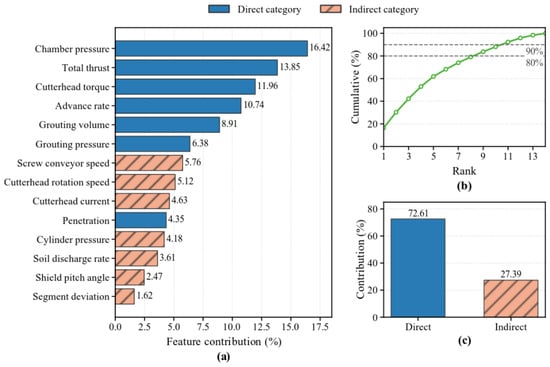
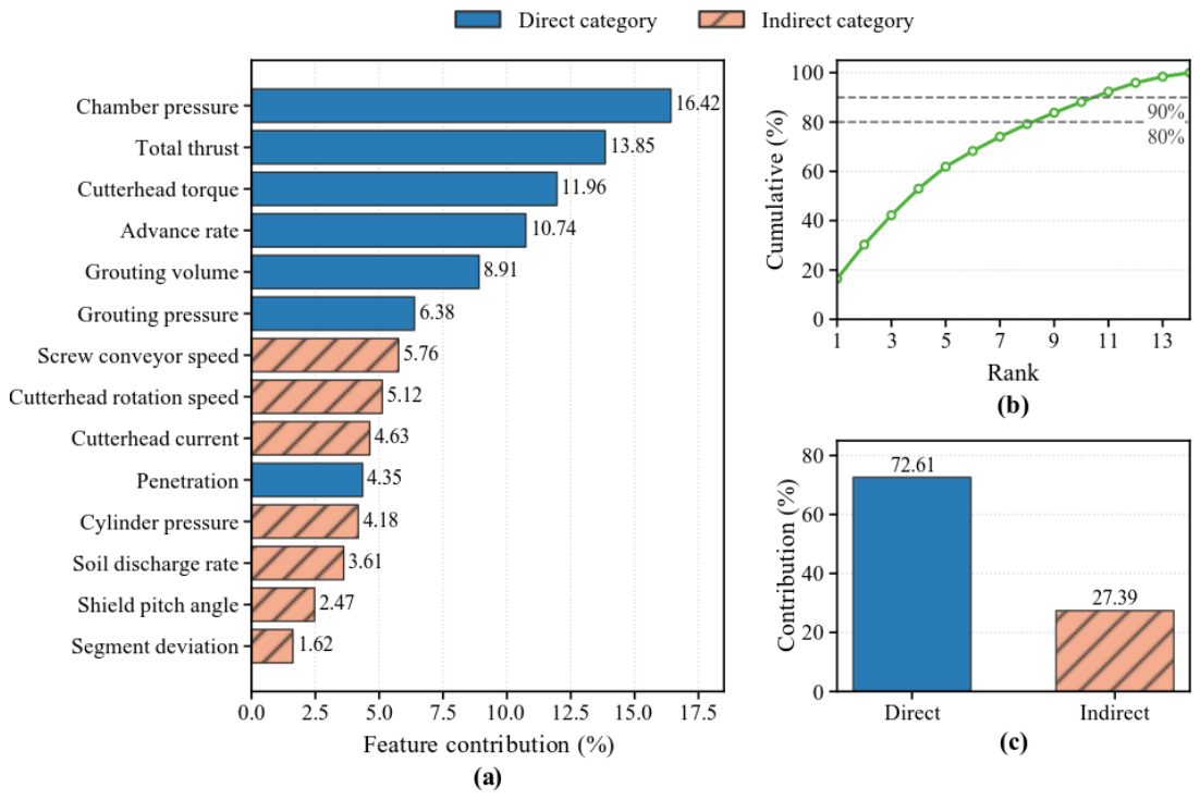
Figure 1 presents the RF-MDI importance ranking and cumulative importance of the 14 candidate tunneling parameters. Chamber pressure shows the highest importance at 16.42%, followed by total thrust, cutterhead torque, and advance rate at 13.85%, 11.96%, and 10.74%, respectively. Grouting volume and grouting pressure contribute 8.91% and 6.38%. These parameters mainly characterize face support, shield advancement, cutterhead excavation, and tail-void grouting, which are closely associated with ground disturbance during shield construction.

Figure 1. RF-MDI feature importance analysis of tunneling parameters: (a) importance ranking of the 14 candidate parameters; (b) cumulative importance of the ranked parameters; (c) aggregated importance of directly and indirectly influential parameter categories.

The 80% and 90% lines in Figure 1b serve as reference levels for cumulative importance. According to the engineering classification introduced in Section 2.2, the seven directly influential parameters account for 72.61% of the total MDI importance, while the seven indirectly influential parameters account for 27.39%. These proportions characterize the relative importance distribution of the two engineering groups for the present dataset and RF model.

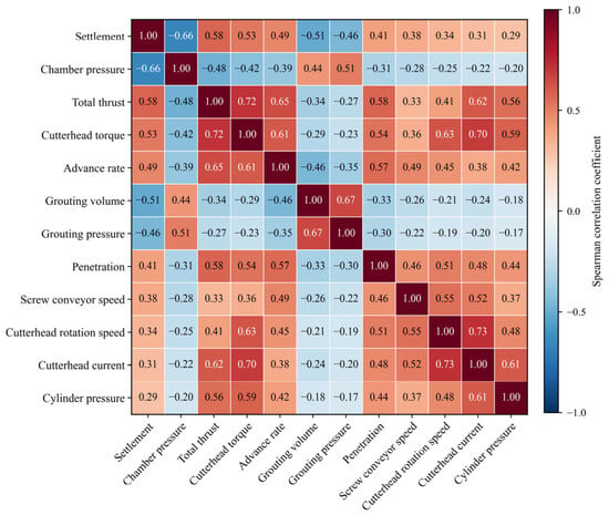
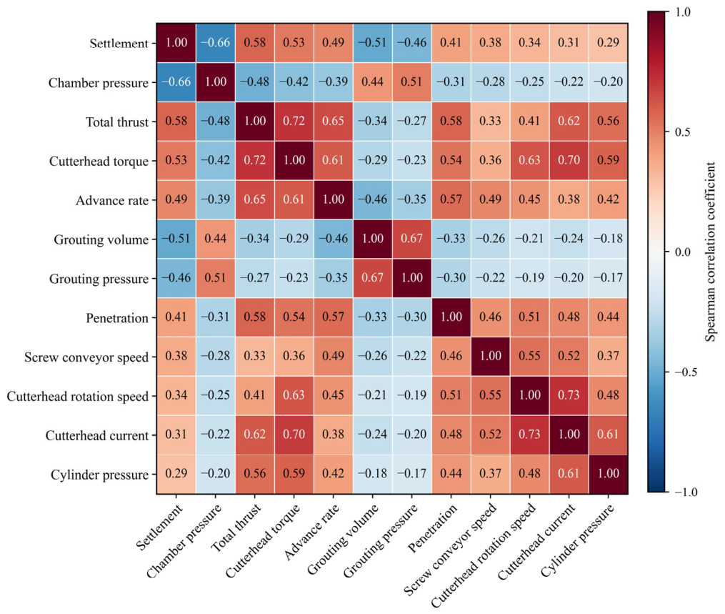
Figure 2 further illustrates the correlations among tunneling parameters. The correlation coefficients of total thrust–cutterhead torque, cutterhead current–cutterhead rotation speed, and cutterhead torque–cutterhead current reach 0.72, 0.73, and 0.70, respectively, indicating substantial shared information among several operational variables. Accordingly, MDI importance is combined with SHAP or permutation importance, SMA-based feature selection, and Spearman correlation to improve the robustness of key-parameter identification.

Figure 2. Correlation heatmap of tunneling parameters.

Considering these correlations, TreeSHAP is further employed as an independent assessment of the RF-MDI ranking. Table 3 reports the RF-MDI importance and ranking, the mean and standard deviation of normalized SHAP importance obtained from 20 repeated RF runs, the SHAP ranking, top-10 occurrence frequency, SMA selection frequency, and the Spearman correlation between each parameter and cumulative surface settlement.

Table 3. Identification results of key tunneling parameters.

Parameter	RF-MDI (%)	MDI Rank	SHAP Importance (%, Mean ± SD)	SHAP Rank	Top-10 Frequency (%)	SMA Frequency (%)	Spearman Coefficient	Retained
Chamber pressure	16.42	1	15.86 ± 0.62	1	100	100	−0.66	1
Total thrust	13.85	2	13.42 ± 0.55	2	100	100	0.58	1
Cutterhead torque	11.96	3	11.51 ± 0.48	3	100	95	0.53	1
Advance rate	10.74	4	10.26 ± 0.44	4	100	95	0.49	1
Grouting volume	8.91	5	9.18 ± 0.41	5	100	95	−0.51	1
Grouting pressure	6.38	6	6.72 ± 0.35	6	100	90	−0.46	1
Screw conveyor speed	5.76	7	5.58 ± 0.33	7	95	90	0.38	1
Cutterhead rotation speed	5.12	8	5.31 ± 0.31	8	95	85	0.34	1
Cutterhead current	4.63	9	4.69 ± 0.28	10	85	80	0.31	1
Penetration	4.35	10	4.91 ± 0.29	9	90	85	0.41	1
Cylinder pressure	4.18	11	4.24 ± 0.30	11	30	40	0.29	0
Soil discharge rate	3.61	12	3.77 ± 0.27	12	20	30	0.27	0
Shield pitch angle	2.47	13	2.36 ± 0.22	13	5	15	0.24	0
Segment deviation	1.62	14	2.19 ± 0.19	14	0	10	0.22	0

The RF-MDI and TreeSHAP rankings show very high consistency, with a Spearman rank correlation of 0.996 and a Top-10 overlap of 100%. Across 20 repeated RF runs, the retained parameters appear in the Top-10 with frequencies of 85–100%, whereas the excluded parameters show substantially lower frequencies of 0–30%. The repeated SMA searches present the same overall pattern, further supporting the stability of the selected feature set.

For variables near the selection boundary, cylinder pressure has an RF-MDI importance of 4.18%, close to cutterhead current (4.63%) and penetration (4.35%). However, its Top-10 frequency is only 30%, compared with 85% and 90% for the latter two variables. Based on the combined evidence from RF-MDI, TreeSHAP, repeated-run stability, SMA selection frequency, Spearman correlation, and engineering interpretation, the final 10 key tunneling parameters are retained for subsequent model development.

2.5. Determination of Key Parameter Input Schemes

Based on the key tunneling parameter identification results in Section 2.4, different feature-input schemes are constructed to evaluate the influence of key-parameter selection on surface settlement prediction. The model inputs consist of geometric, geological, and tunneling parameters, with five geometric features and six geological features. The complete tunneling-parameter set contains 14 candidate variables, among which 10 are retained as key tunneling parameters for subsequent model analysis.

Four input schemes are established, including full-feature input, key-parameter input, tunneling-parameter-only input, and key tunneling-parameter-only input, as summarized in Table 4. The full-feature scheme combines five geometric parameters, six geological parameters, and 14 tunneling parameters, resulting in an input dimension of 25. The key-parameter scheme retains the geometric and geological information together with 10 key tunneling parameters, resulting in an input dimension of 21. Two additional schemes containing 14 tunneling parameters and 10 key tunneling parameters are introduced to further evaluate the predictive contribution of tunneling variables.

Table 4. Configuration of different model input schemes.

Input Scheme	Geometric Parameter Dimension	Geological Parameter Dimension	Named Tunneling Candidates	Provisional Input Dimension	Original Key Share (%)
Full-feature input	5	6	14	25	40.00
Key-parameter input	5	6	10	21	47.62
Tunneling-parameter-only input	0	0	14	14	71.43
Key tunneling-parameter-only input	0	0	10	10	100.00

All input schemes use the same retained samples and identical training, validation, and test partitions to ensure a consistent basis for model comparison. The key-feature configuration is determined from the multi-method feature-identification results obtained from the training and validation data, and prediction performance is subsequently evaluated on the fixed test set. This design enables the respective contributions of geometric and geological information, the complete tunneling-parameter set, and the selected key tunneling parameters to be quantitatively compared.

3. Construction of a Transfer Multilayer Perceptron Model

3.1. Principle of the Multilayer Perceptron Model

A Multilayer Perceptron (MLP) is a feedforward neural network composed of an input layer, multiple hidden layers, and an output layer [37]. In this study, the MLP is employed to establish a nonlinear mapping between multi-source shield construction features and surface settlement responses. For shield ring state $k$ and monitoring point $p$, the model takes the corresponding tunneling, geometric, and geological features as inputs and predicts the cumulative surface settlement at monitoring point $p$: $X_{k,p}\to y_{k,p}$. Each sample corresponds to a time-aligned ring-monitoring point pair. By arranging the predicted values at the same monitoring location according to shield advancement, the longitudinal evolution of surface settlement can be further obtained.

The input feature vector of the $i$-th sample is defined as

$$X_i=[x_{i1},x_{i2},\dots ,x_{id}{]}^T$$

(11)

where $d$ is the number of input features and $y_i$ denotes the measured cumulative surface settlement of the corresponding sample. For an MLP containing $L$ hidden layers, forward propagation at layer $l$ is expressed as

$$h_i^{\left(l\right)}=f\left(W^{\left(l\right)}{h}_i^{(l-1)}+b^{\left(l\right)}\right), l=1,\dots ,L$$

(12)

where $h_i^{\left(0\right)}=X_i$, $W^{\left(l\right)}$ and $b^{\left(l\right)}$ are the weight matrix and bias vector of layer $l$, respectively, and $f(\cdot )$ denotes the activation function.

The Rectified Linear Unit (ReLU) is adopted for the hidden layers:

$$f\left(z\right)=\max (0,z)$$

(13)

The output layer uses a linear mapping to obtain the predicted cumulative surface settlement:

$${\widehat{y}}_i=W^{(L+1)}{h}_i^{\left(L\right)}+b^{(L+1)}$$

(14)

where ${\widehat{y}}_i$ denotes the predicted settlement of the $i$-th sample, and $W^{(L+1)}$ and $b^{(L+1)}$ are the weight matrix and bias of the output layer, respectively.

The model is trained using a loss function combining mean squared error and L2 regularization:

$$\mathcal{L}={\displaystyle \frac{1}{N}}{\sum }_{i=1}^N{\left(y_i-{\widehat{y}}_i\right)}^2+\lambda {\Vert \theta \Vert }_2^2$$

(15)

where $N$ is the number of training samples, $\theta$ denotes the trainable parameters of the MLP, and $\lambda$ is the regularization coefficient. During training, gradients are calculated through backpropagation and the model parameters are iteratively updated by the optimization algorithm, enabling the MLP to learn the nonlinear relationship between shield construction features and cumulative surface settlement.

3.2. Input Feature Design Based on Key Parameters

The design of input features directly influences model training efficiency and prediction performance. Shield construction data contain geometric, geological, and tunneling parameters with different levels of information contribution and inter-feature correlation. Based on the key-parameter identification results in Section 2.5, two principal input configurations are adopted: full-feature input and key-feature input. Both configurations share the same geometric information, geological information, and prediction target, while differing in the tunneling-parameter subset.

The full-feature input combines geometric parameters $X_g$, geological parameters $X_{\mathrm{g}\mathrm{e}\mathrm{o}}$, and the complete tunneling-parameter set $X_t$:

$$X_{\mathrm{f}\mathrm{u}\mathrm{l}\mathrm{l}}=[X_g,X_{\mathrm{g}\mathrm{e}\mathrm{o}},X_t]$$

(16)

This configuration retains comprehensive multi-source construction information and serves as the baseline for subsequent model comparison.

The key-feature input retains the same geometric and geological parameters together with the key tunneling-parameter set $X_k$ identified in Section 2.3 and Section 2.4:

$$X_{\mathrm{k}\mathrm{e}\mathrm{y}}=[X_g,X_{\mathrm{g}\mathrm{e}\mathrm{o}},X_k]$$

(17)

Comparison between the two configurations enables evaluation of the contribution of key-parameter selection to input dimensionality reduction, information compactness, and effective feature representation.

Before model training, the training, validation, and test sets are fixed according to the grouped spatial-block partitioning strategy described in Section 2.3. For the $j$-th input feature, standardization is performed as

$${\tilde{x}}_{ij}={\displaystyle \frac{x_{ij}-{\mu }_j}{{\sigma }_j}}$$

(18)

where $x_{ij}$ is the $j$-th feature of the $i$-th sample, and ${\mu }_j$ and ${\sigma }_j$ are the mean and standard deviation estimated from the training data. The same training-derived statistics are subsequently applied to the corresponding validation and test sets. The source-pretrained network and its transferred target-domain model use the same source-training feature scale to preserve consistency between the input space and transferred parameters, whereas target-only baseline models use statistics derived from the target-domain training data.

3.3. Source-Domain Model Training and Optimization

The source domain is used to learn transferable representations of the relationship between shield construction features and surface settlement. The source section is determined according to engineering-condition differences and the quantitative domain-distribution analysis presented in Section 3.4.1. After temporal matching, spatial grouping, and preprocessing, the retained source-domain dataset is expressed as

$$D_s={\left\{\left(X_i^s,y_i^s\right)\right\}}_{i=1}^{N_s}$$

(19)

where $X_i^s$ and $y_i^s$ denote the input features and cumulative surface settlement of the $i$-th source-domain sample, respectively, and $N_s$ is the number of retained source-domain samples. The source data are divided into grouped spatial-block training, validation, and test subsets. The training subset is used for parameter learning, the validation subset supports hyperparameter selection and early stopping, and the test subset provides independent source-domain performance evaluation.

Source-domain MLP training includes feature construction, standardization, network configuration, model optimization, and validation-based model selection. The network configuration is mainly determined by the number of hidden layers, neurons per layer, learning rate, batch size, and training epochs. Validation loss is used for model selection, and early stopping retains the parameter state associated with the best validation performance.

The source-domain optimization objective is formulated as

$${\theta }_s^{*}=\arg \underset{{\theta }_s}{\mathrm{m}\mathrm{i}\mathrm{n}}\left[{\displaystyle \frac{1}{N_{s,\mathrm{t}\mathrm{r}}}}{\sum }_{i=1}^{N_{s,\mathrm{t}\mathrm{r}}}{\left(y_i^s-{\widehat{y}}_i^s\right)}^2+\lambda {\Vert {\theta }_s\Vert }_2^2\right]$$

(20)

where ${\theta }_s$ denotes the trainable parameters of the source-domain MLP, $N_{s,\mathrm{t}\mathrm{r}}$ is the number of source-domain training samples, ${\widehat{y}}_i^s$ is the predicted settlement, and $\lambda$ is the regularization coefficient. The optimized source-domain parameters ${\theta }_s^{*}$ are subsequently used to initialize the target-domain model, providing the basis for cross-condition feature transfer and target-domain fine-tuning.

3.4. Transfer Learning Strategy Across Operating Conditions

3.4.1. Target Domain Definition

The target domain corresponds to the shield section in which construction-stage settlement prediction is performed using a limited amount of monitoring data. After temporal matching, spatial grouping, and preprocessing, the target-domain dataset is expressed as

$$D_t={\left\{\left(X_i^t,y_i^t\right)\right\}}_{i=1}^{N_t}$$

(21)

where $X_i^t$ and $y_i^t$ denote the input features and cumulative surface settlement of the $i$-th target-domain sample, respectively, and $N_t$ is the number of retained target-domain samples. The target-domain data are divided into fine-tuning, validation, and test subsets according to continuous ring blocks and monitoring sections. The fine-tuning subset is used for parameter adaptation, the validation subset supports model selection, and the test subset is used for final performance evaluation.

Cross-condition transfer is established on measurable distribution differences between the source and target domains, which can be expressed as

$$P_s(X,Y)\ne P_t(X,Y)$$

(22)

where $P_s(X,Y)$ and $P_t(X,Y)$ denote the joint distributions of input features and settlement responses in the source and target domains, respectively.

Domain differences are evaluated from both individual feature distributions and the overall feature space. Probability-density distributions of key tunneling parameters are first compared to characterize changes in construction conditions. t-SNE is then employed to project the high-dimensional feature space into two dimensions and visualize the distribution structure of source- and target-domain samples [38]. Maximum Mean Discrepancy (MMD) is further used to quantify the overall distribution distance between the two domains [39]. All distribution analyses adopt a consistent feature-scaling scheme, and spatial-block resampling is used to evaluate the stability of the resulting domain-difference measures. The combination of visual and quantitative analyses provides the data basis for cross-condition domain definition.

3.4.2. Parameter Transfer

The Transfer Multilayer Perceptron (T-MLP) implements cross-condition knowledge transfer through source-domain parameter initialization and selective target-domain fine-tuning. The network parameters obtained from source-domain training are transferred to the target model as initial values, after which selected shallow layers are retained while the remaining layers are adapted to the target condition.

The optimized source-domain parameters are denoted as

$${\theta }_s^{*}={\left\{W_s^{\left(l\right)},b_s^{\left(l\right)}\right\}}_{l=1}^{L+1}$$

(23)

and the target-domain model is initialized as

$${\theta }_t^{\left(0\right)}={\theta }_s^{*}$$

(24)

The transferred parameters are further divided into the frozen subset ${\theta }_f^s$ and the trainable subset ${\theta }_u^s$. During target-domain adaptation, the frozen parameters remain at their source-pretrained values,

$${\theta }_f={\theta }_f^s$$

(25)

while the remaining parameters are initialized from ${\theta }_u^s$ and optimized using the target-domain fine-tuning samples. The target-domain objective is formulated as

$${\theta }_u^{*}=\arg \underset{{\theta }_u}{\mathrm{m}\mathrm{i}\mathrm{n}}\left[{\displaystyle \frac{1}{N_{t,\mathrm{t}\mathrm{r}}}}{\sum }_{i=1}^{N_{t,\mathrm{t}\mathrm{r}}}{\left(y_i^t-f(X_i^t;{\theta }_f^s,{\theta }_u)\right)}^2+\alpha {\Vert {\theta }_u-{\theta }_u^s\Vert }_2^2\right]$$

(26)

where $N_{t,\mathrm{t}\mathrm{r}}$ is the number of target-domain fine-tuning samples, ${\theta }_u^{*}$ denotes the optimized trainable parameters, and $\alpha$ is the transfer regularization coefficient. The second term constrains parameter deviation from the source-pretrained state, allowing the model to preserve transferable representations while adapting to the target construction condition.

The proposed T-MLP configuration retains the first hidden layer at its source-pretrained state and fine-tunes the subsequent hidden layers and output layer. An all-layer fine-tuning configuration is also established using the same source initialization, target-domain data, and training conditions. Comparison between these transfer configurations and the corresponding baseline models is used to quantify the effects of shallow-feature retention and deeper-layer adaptation on cross-condition settlement prediction.

3.5. Construction Process and Evaluation Metrics of the T-MLP Model

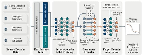
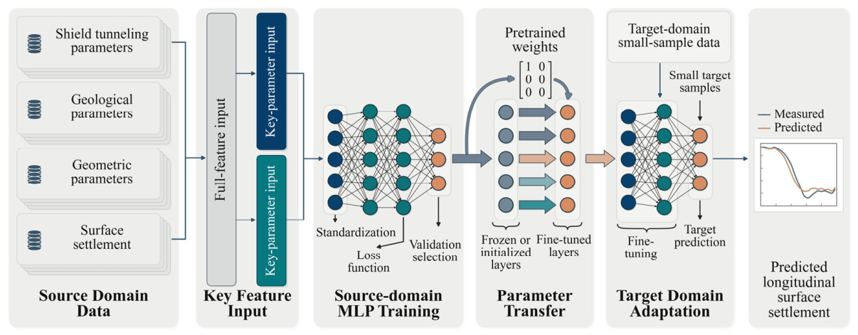
After key-parameter input design, source-domain model training, and cross-condition parameter transfer, the complete T-MLP framework is established as illustrated in Figure 3. The workflow consists of multi-source data alignment, spatial-block partitioning, data preprocessing and key-feature identification, source-domain MLP pretraining, parameter transfer, target-domain fine-tuning, and final test-set evaluation. The training set is used for model parameter learning, the validation set supports feature selection, hyperparameter optimization, and model selection, and the fixed test set provides the final assessment of prediction performance.

Figure 3. Workflow of the T-MLP model construction process.

To comprehensively evaluate surface settlement prediction performance, Mean Absolute Error (MAE), Root Mean Square Error (RMSE), the coefficient of determination (R²), and Maximum Absolute Error (MaxAE) are adopted as evaluation metrics [19,23].

MAE measures the average absolute deviation between predicted and observed settlement values:

$$MAE={\displaystyle \frac{1}{N}}{\sum }_{i=1}^N|y_i-{\widehat{y}}_i|$$

(27)

RMSE places greater emphasis on relatively large prediction errors and reflects the model’s ability to control local settlement deviations:

$$RMSE=\sqrt{{\displaystyle \frac{1}{N}}{\sum }_{i=1}^N(y_i-{\widehat{y}}_i{)}^2}$$

(28)

R² evaluates the overall capability of the model to explain variations in the measured surface settlement:

$$R^2=1-{\displaystyle \frac{{\sum }_{i=1}^N(y_i-{\widehat{y}}_i{)}^2}{{\sum }_{i=1}^N(y_i-\overline{y}{)}^2}}$$

(29)

MaxAE characterizes the largest local prediction deviation within the test set:

$$MaxAE=\underset{1\le i\le N}{\max }|y_i-{\widehat{y}}_i|$$

(30)

where $y_i$ and ${\widehat{y}}_i$ are the measured and predicted settlement values of the $i$-th test sample, respectively, $\overline{y}$ is the mean measured settlement of the test set, and $N$ is the number of test samples. MAE, RMSE, and MaxAE are expressed in millimeters, whereas R² is dimensionless. Model effectiveness is evaluated jointly through prediction errors, goodness of fit, and performance improvements relative to the baseline models. To further assess result stability, uncertainty is evaluated through grouped resampling of independent ring blocks or monitoring sections together with repeated model training.

4. Results Analysis and Discussion

4.1. Experimental Setup and Parameter Configuration

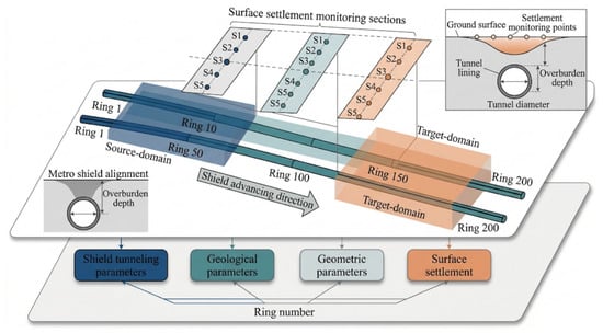
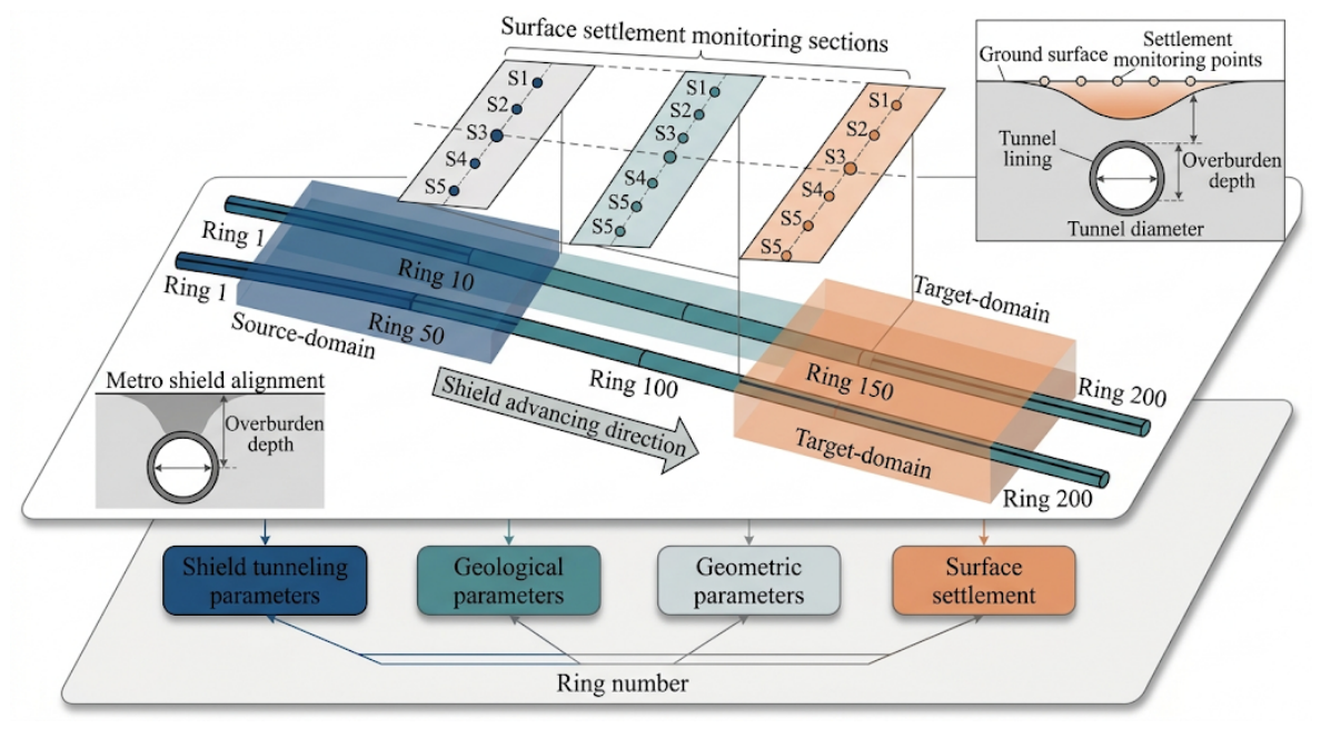
The case study is conducted using the Chengdu Metro Line 18 shield-driven interval described in Section 2.1. According to the construction conditions and the domain-distribution analysis in Section 3.4.1, Rings 1–50 are used as the source-domain section and Rings 150–200 as the target-domain section. Settlement observations are aligned with shield-ring states using the timestamp-matching procedure described in Section 2.3, and continuous ring intervals together with monitoring sections are used as spatial grouping units. Figure 4 illustrates the shield interval and surface monitoring layout, with five transverse monitoring points, S1–S5, arranged at each monitoring section.

Figure 4. Schematic diagram of the engineering section and monitoring point layout.

For each ring-monitoring point sample, the model inputs consist of tunneling, geometric, and geological features, while the output is the cumulative surface settlement at the corresponding monitoring point. Training, validation, and test subsets are constructed using the same grouped spatial-block strategy, and identical eligible samples and a fixed test set are used for all model comparisons.

Support Vector Regression (SVR), Random Forest (RF), and Multilayer Perceptron (MLP) are selected as baseline models and compared with T-MLP. For SVR, the radial basis function kernel is adopted, with $C\in \{10, 50, 100, 200\}$, $\gamma \in \{0.001, 0.01, \mathrm{0.1,1}\}$, and $\epsilon \in \{0.01, 0.05, 0.10\}$. For RF, the number of trees is selected from $\{100, 200, 300, 500\}$, the maximum depth from $\{5, 10, 15,\mathrm{u}\mathrm{n}\mathrm{l}\mathrm{i}\mathrm{m}\mathrm{i}\mathrm{t}\mathrm{e}\mathrm{d}\}$, and the minimum number of samples per leaf from $\{1, 2, 4, 6\}$, together with optimization of the maximum number of features.

For the MLP, two- and three-hidden-layer architectures are considered, with the number of neurons selected from $\{32, 64, 128\}$. ReLU is used as the hidden-layer activation function. The learning rate is selected from $\{0.001, 0.0005, 0.0001\}$, the batch size from $\{16, 32, 64\}$, and the maximum number of training epochs is set to 500. Early stopping is employed for model selection.

The source-domain data are divided into training, validation, and test subsets using grouped spatial blocks, with 70%, 15%, and 15% serving as the nominal allocation ratios. For the target domain, four nested fine-tuning subsets containing 54, 90, 120, and 180 samples are constructed from a common target-domain training pool: $D_{54}\subset D_{90}\subset D_{120}\subset D_{180}$. All four experiments share the same target-domain validation set and fixed test set, allowing the influence of target-domain sample size on transfer performance to be evaluated consistently.

For T-MLP, the target model is initialized using the source-pretrained parameters. The first hidden layer retains its source-domain parameters, while the subsequent hidden layers and output layer are fine-tuned using target-domain samples. The target-domain learning rate is set to 0.0001, and the early-stopping patience is 30 epochs. An all-layer fine-tuning configuration is also included to evaluate the contribution of shallow-layer parameter retention. All models are compared using identical data partitions, evaluation metrics, and test samples. All computational experiments were implemented in Python (version 3.11.9). Scikit-learn (version 1.4.2) was employed for SVR and RF modeling, while PyTorch (version 2.3.1) was used to construct and train the MLP and T-MLP models. SHAP (version 0.46.0) was adopted for TreeSHAP-based feature importance analysis, and SMA-based optimization was implemented using custom Python scripts.

4.2. Prediction Performance Analysis Under Different Feature Input Schemes

To evaluate the influence of key tunneling parameter selection on prediction performance, SVR, RF, and MLP are trained and tested using full-feature and key-feature inputs. Both schemes use identical ring-monitoring point samples, grouped spatial-block partitions, and a fixed test set. Data standardization and feature selection are performed using the training data. The quantitative results under the two input schemes are summarized in Table 5.

Table 5. Comparison of prediction errors under different feature input schemes.

Model	Input Scheme	MAE (mm)	RMSE (mm)	R2	Standard Deviation of MAE (mm)
SVR	Full-feature input	3.62	4.71	0.842	0.31
SVR	Key-feature input	3.18	4.12	0.881	0.24
RF	Full-feature input	3.05	3.94	0.891	0.26
RF	Key-feature input	2.72	3.54	0.913	0.21
MLP	Full-feature input	2.68	3.49	0.916	0.28
MLP	Key-feature input	2.21	2.91	0.941	0.18

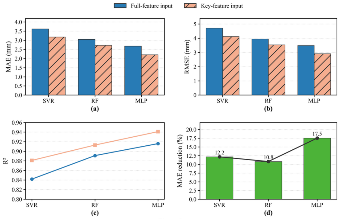
Key-feature input improves the prediction performance of all three models. For SVR, MAE and RMSE decrease by 12.15% and 12.53%, respectively. The corresponding reductions for RF are 10.82% and 10.15%, while MLP achieves reductions of 17.54% and 16.62%. Meanwhile, the R² of MLP increases from 0.916 to 0.941, and the standard deviation of MAE decreases from 0.28 to 0.18 mm.

These results indicate that key-parameter selection improves information compactness while reducing the input dimension. The improvement is particularly pronounced for MLP, suggesting that reducing redundant tunneling variables facilitates more effective learning of the nonlinear relationship between shield construction features and surface settlement.

4.3. Comparison of Predictive Performance Across Different Models

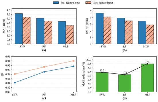
Under different feature input schemes, the predictive performance of SVR, RF, and MLP is further compared. Figure 5 presents the MAE, RMSE, and R² of the three models under full-feature and key-feature inputs, together with the corresponding MAE reduction achieved by key-feature selection.

Figure 5. Comparison of prediction performance under different feature input schemes: (a) MAE; (b) RMSE; (c) R²; (d) MAE reduction achieved by key-feature input.

Figure 5 shows that key-feature input consistently reduces MAE and RMSE while increasing R² for all three models. Among them, MLP achieves the lowest prediction errors and the highest R². The corresponding evaluation metrics under key-feature input, including the maximum absolute error, are further summarized in Table 6.

Table 6. Evaluation metrics of different prediction models.

Model	MAE (mm)	RMSE (mm)	R2	MaxAE (mm)
SVR	3.18	4.12	0.881	12.47
RF	2.72	3.54	0.913	10.36
MLP	2.21	2.91	0.941	8.72

MLP achieves an MAE of 2.21 mm, an RMSE of 2.91 mm, a MaxAE of 8.72 mm, and an R² of 0.941. Relative to SVR, its MAE and RMSE decrease by 30.50% and 29.37%, respectively. Relative to RF, the corresponding reductions are 18.75% and 17.80%.

These results demonstrate the strong overall capability of MLP to represent the nonlinear mapping between multi-source shield construction features and cumulative surface settlement. MLP is therefore adopted as the backbone network for subsequent cross-condition parameter transfer. Stage-specific differences between RF and MLP are further analyzed in Section 4.6.

4.4. Cross-Condition Prediction Performance Analysis of the T-MLP Model

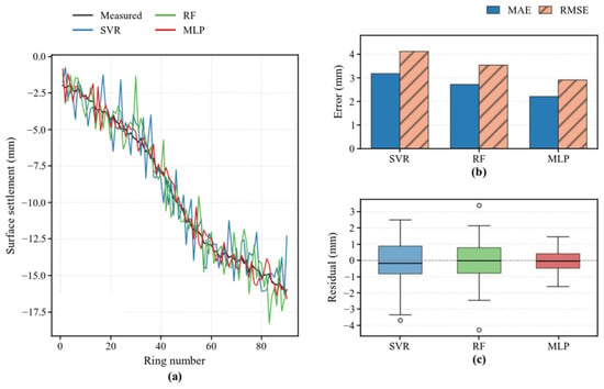
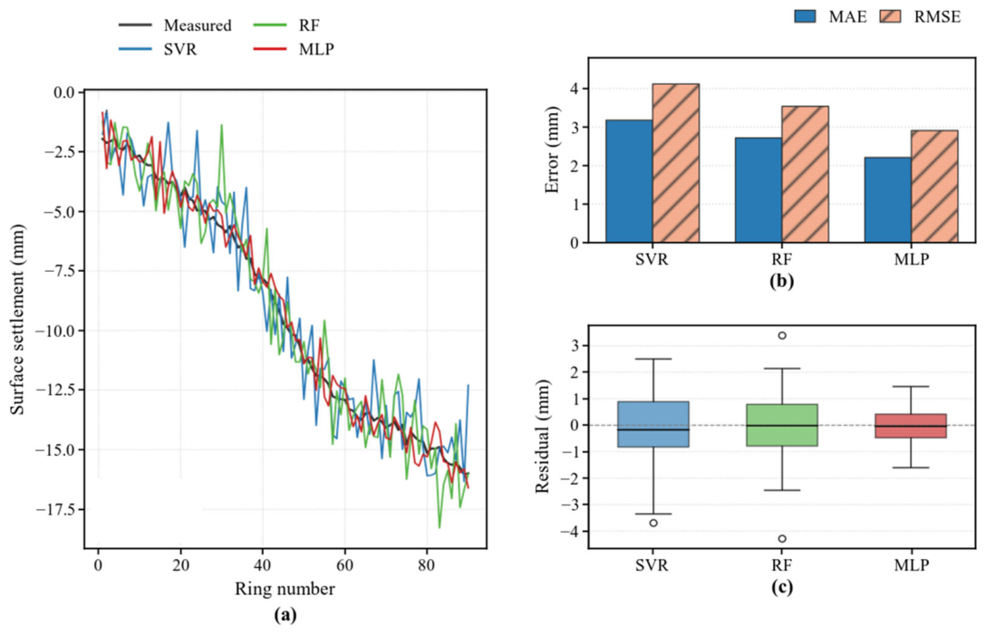
To evaluate the contributions of source-domain knowledge transfer and target-domain adaptation, Source-only MLP, target-domain SVR, RF and MLP, and T-MLP are compared using the same fixed target-domain test set. Figure 6 presents the measured and predicted settlement responses under the different cross-condition prediction strategies.

Figure 6. Comparison of prediction performance among different baseline models: (a) measured and predicted surface settlement; (b) comparison of MAE and RMSE; (c) distributions of prediction residuals.

Figure 6 shows progressively closer agreement with the measured settlement after target-domain training and parameter transfer. The quantitative prediction performance of the different strategies is summarized in Table 7.

Table 7. Cross-condition prediction performance of different models.

Model	Training Strategy	MAE (mm)	RMSE (mm)	R2	MAE Reduction Rate (%)
Source-only MLP	Source-domain direct prediction	5.26	6.51	0.643	0.00
SVR	Target-domain small-sample training	4.21	5.32	0.731	19.96
RF	Target-domain small-sample training	3.86	4.91	0.768	26.62
MLP	Target-domain small-sample training	3.73	4.72	0.786	29.09
T-MLP	Source pretraining and target fine-tuning	3.18	4.08	0.852	39.54

The Source-only MLP produces an MAE of 5.26 mm, an RMSE of 6.51 mm, and an R² of 0.643 in the target section, reflecting the influence of changing construction conditions on predictive performance. After source pretraining and target-domain fine-tuning, T-MLP reduces the MAE to 3.18 mm and the RMSE to 4.08 mm, while R² increases to 0.852. Relative to the Source-only MLP, MAE and RMSE decrease by 39.54% and 37.33%, respectively.

Compared with target-domain SVR, RF, and MLP, T-MLP reduces MAE by 24.47%, 17.62%, and 14.75%, respectively, and RMSE by 23.31%, 16.90%, and 13.56%. The consistent improvements across the evaluation metrics indicate that source-domain pretraining provides effective parameter initialization and target-domain fine-tuning further enhances adaptation to the new construction condition.

4.5. Effect of Target-Domain Sample Size on Transfer Performance

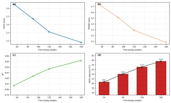
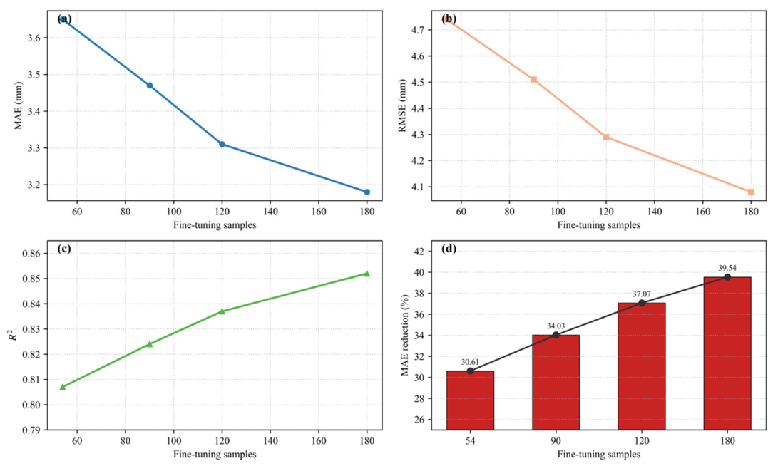
The amount of available target-domain monitoring data directly affects the degree of target adaptation. Four nested fine-tuning subsets containing 54, 90, 120, and 180 samples are therefore constructed from the same target-domain training pool: $D_{54}\subset D_{90}\subset D_{120}\subset D_{180}$. All four configurations use the same validation set and fixed test set. Figure 7 illustrates the variation of MAE, RMSE, and R² with the number of target-domain fine-tuning samples.

Figure 7. Effect of target-domain sample size on the performance of the T-MLP model: (a) MAE; (b) RMSE; (c) coefficient of determination (R²); (d) MAE reduction relative to the source-only MLP.

As the number of fine-tuning samples increases from 54 to 90, 120, and 180, MAE decreases from 3.65 to 3.47, 3.31, and 3.18 mm, respectively. RMSE decreases from 4.74 to 4.51, 4.29, and 4.08 mm, while R² increases from 0.807 to 0.824, 0.837, and 0.852. Relative to the 54-sample configuration, the 180-sample configuration reduces MAE and RMSE by 12.88% and 13.92%, respectively.

The successive MAE improvements are 0.18, 0.16, and 0.13 mm, indicating continued performance gains together with a gradual reduction in marginal improvement. With only 54 target-domain samples, T-MLP already achieves a 30.61% MAE reduction relative to the Source-only MLP, demonstrating the effectiveness of parameter transfer under limited target-domain monitoring data.

4.6. Analysis of Longitudinal Surface Settlement Curve Prediction Performance

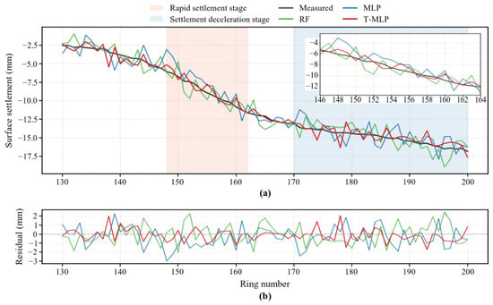
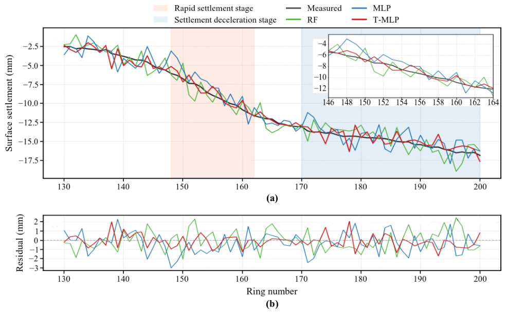
In addition to aggregate error metrics, the longitudinal settlement evolution provides a direct representation of model performance as the shield approaches, passes, and moves away from the monitoring location. Pointwise predictions at the same monitoring location are connected according to shield advancement to form the longitudinal surface settlement curve. Figure 8 compares the prediction results of RF, MLP, and T-MLP.

Figure 8. Comparison of longitudinal ground surface settlement predictions: (a) measured and predicted settlement curves with an enlarged view of the rapid settlement stage; (b) prediction residuals of RF, MLP, and T-MLP across shield ring numbers.

Figure 8 shows that all three models capture the overall longitudinal settlement evolution, while their local responses differ in regions with rapid settlement variation. To quantify these stage-specific differences, the settlement process is divided into a rapid settlement stage and an attenuation stage according to the relative shield-face position and settlement-rate evolution, with the stage boundaries fixed before model evaluation. The corresponding prediction errors are summarized in Table 8.

Table 8. Prediction errors at different settlement stages.

Model	Rapid-Stage MAE (mm)	Rapid-Stage RMSE (mm)	Attenuation-Stage MAE (mm)	Attenuation-Stage RMSE (mm)
RF	4.38	5.26	3.01	3.74
MLP	5.02	6.08	2.78	3.43
T-MLP	4.21	5.04	2.23	2.86

All three models exhibit larger prediction errors during the rapid settlement stage, reflecting the greater modeling difficulty associated with larger settlement gradients as the shield approaches and passes the monitoring location. RF achieves a rapid-stage MAE of 4.38 mm compared with 5.02 mm for MLP, while MLP provides stronger overall performance across the complete test set. This stage-dependent behavior reflects different modeling characteristics: RF responds effectively to some localized rapid variations, whereas MLP provides stronger overall representation of the multivariable nonlinear settlement process.

T-MLP achieves an MAE of 4.21 mm and an RMSE of 5.04 mm during the rapid settlement stage, with corresponding values of 2.23 and 2.86 mm during the attenuation stage. These values are lower than the corresponding RF and MLP results in both stages. The combination of source-domain parameter initialization and target-domain adaptation therefore improves model adaptability across different stages of settlement evolution.

4.7. Ablation Study

To quantify the individual contributions of key-feature selection, source-domain pretraining, target-domain adaptation, and shallow-layer parameter retention, six controlled configurations are evaluated. All configurations use identical target-domain training, validation, and fixed test sets together with consistent backbone architectures and training conditions. The results are summarized in Table 9.

Table 9. Ablation results of the T-MLP framework.

Configuration	Input and Transfer Strategy	MAE (mm)	RMSE (mm)	R2	MaxAE (mm)
Target-only MLP	Full features	4.06	5.14	0.746	13.42
Target-only MLP	Key features	3.73	4.72	0.786	12.18
T-MLP	Full features + first hidden layer frozen	3.44	4.39	0.823	11.05
T-MLP	Key features + all layers fine-tuned	3.29	4.20	0.840	10.36
Proposed T-MLP	Key features + first hidden layer frozen	3.18	4.08	0.852	9.94
Source-only MLP	Key features + direct target prediction	5.26	6.51	0.643	15.76

Comparison between the two target-only MLP configurations quantifies the contribution of key-feature selection. With key-feature input, MAE decreases from 4.06 to 3.73 mm and RMSE decreases from 5.14 to 4.72 mm, while R² increases from 0.746 to 0.786. The corresponding MAE improvement is 8.13%, confirming the contribution of key tunneling parameter selection under limited target-domain data.

Using the same key-feature input, source-domain initialization followed by all-layer fine-tuning further reduces MAE from 3.73 to 3.29 mm, corresponding to an additional improvement of 11.80%, while R² increases to 0.840. This result demonstrates the contribution of source-domain pretraining to target-domain optimization.

With the first hidden layer retained at its source-pretrained state, the proposed T-MLP achieves an MAE of 3.18 mm, an RMSE of 4.08 mm, and an R² of 0.852. Relative to all-layer fine-tuning, MAE is further reduced by 3.34%. The shallow representations learned from the source domain therefore provide transferable information, while fine-tuning the subsequent hidden layers and output layer enables adaptation to target-condition-specific characteristics.

The Source-only MLP produces an MAE of 5.26 mm, while the final T-MLP achieves 3.18 mm, corresponding to an overall reduction of 39.54%. Taken together, the ablation results show that key-feature selection, source-domain initialization, and target-domain adaptation jointly contribute to cross-condition prediction improvement, with parameter transfer and target-domain fine-tuning providing the principal performance gains.

5. Conclusions

This study develops a T-MLP-based surface settlement prediction framework combining key tunneling parameter identification and parameter transfer to address high-dimensional tunneling inputs, limited monitoring data in target sections, and cross-condition adaptation in shield tunneling. By establishing a unified correspondence among shield rings, monitoring points, and observation timestamps, and integrating grouped spatial-block partitioning, key-feature selection, source-domain pretraining, and target-domain fine-tuning, the proposed framework enables cross-condition prediction of pointwise cumulative surface settlement. The main conclusions are summarized as follows.

(1)

Key tunneling parameters are identified through an integrated assessment combining Random Forest importance, SHAP or permutation importance, SMA-based feature selection, Spearman correlation, and engineering interpretation. Key-feature input improves the prediction performance of all baseline models. The MAE reductions of SVR, RF, and MLP reach 12.15%, 10.82%, and 17.54%, respectively. For MLP, RMSE decreases from 3.49 to 2.91 mm and R² increases from 0.916 to 0.941, demonstrating that key-parameter selection improves feature efficiency and enhances nonlinear settlement representation.

(2)

Distribution differences between construction conditions lead to clear changes in model performance when a source-domain model is transferred to a target section. The Source-only MLP produces an MAE of 5.26 mm, an RMSE of 6.51 mm, and an R² of 0.643 in the target domain. After source-domain parameter transfer and target-domain fine-tuning, T-MLP reduces the MAE to 3.18 mm and RMSE to 4.08 mm, while R² increases to 0.852. Relative to the Source-only MLP, MAE and RMSE decrease by 39.54% and 37.33%, respectively. T-MLP also achieves lower prediction errors than target-domain SVR, RF, and MLP, indicating that source-domain pretraining provides effective initialization for adaptation under limited target-domain data.

(3)

Target-domain sample size has a clear influence on transfer performance. As the number of fine-tuning samples increases from 54 to 180, the MAE of T-MLP decreases from 3.65 to 3.18 mm, RMSE decreases from 4.74 to 4.08 mm, and R² increases from 0.807 to 0.852. The successive MAE improvements gradually decrease from 0.18 to 0.13 mm, indicating continued performance enhancement together with diminishing marginal gains as additional target-domain monitoring data become available. These results demonstrate the effectiveness of parameter transfer under limited target-domain observations.

(4)

Model performance varies across different stages of settlement development. During the rapid settlement stage, RF achieves an MAE of 4.38 mm compared with 5.02 mm for the conventional MLP, reflecting the ability of tree-based models to respond to some localized rapid variations. T-MLP achieves MAE values of 4.21 and 2.23 mm and RMSE values of 5.04 and 2.86 mm during the rapid settlement and attenuation stages, respectively, showing stable prediction performance across different stages of settlement evolution. Together with the ablation analysis, the results indicate that key-feature selection, source-domain initialization, and target-domain adaptation jointly contribute to improved cross-condition prediction.

The present study is based on a single engineering case from Chengdu Metro Line 18, and model performance is influenced by target-domain sample size, spatial partitioning, construction-condition variation, and monitoring temporal resolution. Future research will extend the framework to multiple metro projects, geological conditions, and shield-machine configurations, while incorporating higher-frequency monitoring, physics-informed modeling, and online updating strategies to further improve cross-project generalization and engineering applicability.

References

- Kim, C.Y.; Bae, G.J.; Hong, S.W.; Park, C.H.; Moon, H.K.; Shin, H.S. Neural network based prediction of ground surface settlements due to tunnelling. Comput. Geotech. 2001, 28, 517–547. [Google Scholar] [CrossRef] [Scilit]
- Suwansawat, S.; Einstein, H.H. Artificial neural networks for predicting the maximum surface settlement caused by EPB shield tunneling. Tunn. Undergr. Space Technol. 2006, 21, 133–150. [Google Scholar] [CrossRef] [Scilit]
- Qiao, J.; Fan, Y.; Liu, B.; Li, Y.; Zhang, Y. Predicting the Surface Settlement by Shield Tunneling Based on Modified BP Network. Chin. J. Undergr. Space Eng. 2012, 8, 352–357. (In Chinese) [Google Scholar]
- Pourtaghi, A.; Lotfollahi-Yaghin, M.A. Wavenet ability assessment in comparison to ANN for predicting the maximum surface settlement caused by tunneling. Tunn. Undergr. Space Technol. 2012, 28, 257–271. [Google Scholar] [CrossRef] [Scilit]
- Ocak, I.; Seker, S.E. Calculation of surface settlements caused by EPBM tunneling using artificial neural network, SVM, and Gaussian processes. Environ. Earth Sci. 2013, 70, 1263–1276. [Google Scholar] [CrossRef] [Scilit]
- Wang, F.; Gou, B.; Qin, Y. Modeling tunneling-induced ground surface settlement development using a wavelet smooth relevance vector machine. Comput. Geotech. 2013, 54, 125–132. [Google Scholar] [CrossRef] [Scilit]
- Bouayad, D.; Emeriault, F.; Maza, M. Assessment of ground surface displacements induced by an earth pressure balance shield tunneling using partial least squares regression. Environ. Earth Sci. 2015, 73, 7603–7616. [Google Scholar] [CrossRef] [Scilit]
- Bouayad, D.; Emeriault, F. Modeling the relationship between ground surface settlements induced by shield tunneling and the operational and geological parameters based on the hybrid PCA/ANFIS method. Tunn. Undergr. Space Technol. 2017, 68, 142–152. [Google Scholar] [CrossRef] [Scilit]
- Lai, J.; Qiu, J.; Feng, Z.; Chen, J.; Fan, H. Prediction of Soil Deformation in Tunnelling Using Artificial Neural Networks. Comput. Intell. Neurosci. 2016, 2016, 6708183. [Google Scholar] [CrossRef] [Scilit]
- Goh, A.T.C.; Zhang, W.; Zhang, Y.; Xiao, Y.; Xiang, Y. Determination of earth pressure balance tunnel-related maximum surface settlement: A multivariate adaptive regression splines approach. Bull. Eng. Geol. Environ. 2018, 77, 489–500. [Google Scholar] [CrossRef] [Scilit]
- Chen, R.P.; Zhang, P.; Kang, X.; Zhong, Z.Q.; Liu, Y.; Wu, H.N. Prediction of maximum surface settlement caused by earth pressure balance (EPB) shield tunneling with ANN methods. Soils Found. 2019, 59, 284–295. [Google Scholar] [CrossRef] [Scilit]
- Chen, R.; Zhang, P.; Wu, H.; Wang, Z.; Zhong, Z. Prediction of shield tunneling-induced ground settlement using machine learning techniques. Front. Struct. Civ. Eng. 2019, 13, 1363–1378. [Google Scholar] [CrossRef] [Scilit]
- Zhang, W.G.; Li, H.R.; Wu, C.Z.; Li, Y.Q.; Liu, Z.Q.; Liu, H.L. Soft computing approach for prediction of surface settlement induced by earth pressure balance shield tunneling. Undergr. Space 2021, 6, 353–363. [Google Scholar] [CrossRef] [Scilit]
- Zhang, P.; Wu, H.N.; Chen, R.P.; Chan, T.H.T. Hybrid meta-heuristic and machine learning algorithms for tunneling-induced settlement prediction: A comparative study. Tunn. Undergr. Space Technol. 2020, 99, 103383. [Google Scholar] [CrossRef] [Scilit]
- Mahmoodzadeh, A.; Mohammadi, M.; Daraei, A.; Farid Hama Ali, H.; Kameran Al-Salihi, N.; Mohammed Dler Omer, R. Forecasting maximum surface settlement caused by urban tunneling. Autom. Constr. 2020, 120, 103375. [Google Scholar] [CrossRef] [Scilit]
- Hussaine, S.M.; Mu, L. Intelligent Prediction of Maximum Ground Settlement Induced by EPB Shield Tunneling Using Automated Machine Learning Techniques. Mathematics 2022, 10, 4637, Correction in Mathematics 2023, 11, 1823. https://doi.org/10.3390/math11081823. [Google Scholar] [CrossRef] [Scilit]
- Liu, L.; Zhou, W.; Gutierrez, M. Physics-Informed Ensemble Machine Learning Framework for Improved Prediction of Tunneling-Induced Short- and Long-Term Ground Settlement. Sustainability 2023, 15, 11074. [Google Scholar] [CrossRef] [Scilit]
- Wang, G.; Fang, Q.; Du, J.; Wang, J.; Li, Q. Deep learning-based prediction of steady surface settlement due to shield tunnelling. Autom. Constr. 2023, 154, 105006. [Google Scholar] [CrossRef] [Scilit]
- Shang, W.; Li, Y.; Wei, H.; Qiu, Y.; Chen, C.; Gao, X. Prediction method of longitudinal surface settlement caused by double shield tunnelling based on deep learning. Sci. Rep. 2024, 14, 908. [Google Scholar] [CrossRef] [Scilit]
- Wang, Q.; Shen, C.; Tang, C.; Guo, Z.; Wu, F.; Yang, W. Machine learning-based forecasting of ground surface settlement induced by metro shield tunneling construction. Sci. Rep. 2024, 14, 31795. [Google Scholar] [CrossRef] [Scilit]
- Li, C.; Dias, D. Intelligent prediction and visual optimization of surface settlement induced by earth pressure balance shield tunneling. Tunn. Undergr. Space Technol. 2024, 154, 106138. [Google Scholar] [CrossRef] [Scilit]
- Liu, F.; Liu, W.; Li, A.; Cheng, J.C.P. Geotechnical risk modeling using an explainable transfer learning model incorporating physical guidance. Eng. Appl. Artif. Intell. 2024, 137, 109127. [Google Scholar] [CrossRef] [Scilit]
- Lu, D.; Xu, B.; Kong, F.; Ma, Y.; Du, X. Intelligent Prediction Method for Settlement Curves of Shield Tunnel Based on Machine Learning Algorithms. J. Beijing Univ. Technol. 2024, 50, 1285–1300. (In Chinese) [Google Scholar] [CrossRef]
- Dong, M.; Guan, M.; Wang, K.; Wu, Y.; Fu, Y. Machine Learning-Based Measurement and Prediction of Ground Settlement Induced by Shield Tunneling Undercrossing Existing Tunnels in Composite Strata. Sensors 2025, 25, 1600. [Google Scholar] [CrossRef] [Scilit]
- Yin, Q.; Zhou, Y.; Rao, J. An intelligent prediction method for surface settlement of shield tunnel construction based on CNN-BiLSTM-SA. KSCE J. Civ. Eng. 2025, 29, 100061. [Google Scholar] [CrossRef] [Scilit]
- Wang, G.; Fang, Q.; Wang, J.; Li, Q.; Song, H.; Huang, J. Artificial intelligence prediction of surface settlement induced by twin shields tunnelling. Tunn. Undergr. Space Technol. 2025, 161, 106606. [Google Scholar] [CrossRef] [Scilit]
- Yang, P.; Zhou, J.; Zhang, Y.; Xu, C.; Khandelwal, M.; Huang, S. Ground Settlement Prediction in Urban Tunnelling: Leveraging Metaheuristic-Optimized Random Forest Models. Arab. J. Sci. Eng. 2025, 50, 17025–17044. [Google Scholar] [CrossRef] [Scilit]
- Jin, H.; Xu, Z.; Wang, E.; Liu, X.; Yuan, D. Dynamic response of shield-soil system during shield tunneling: A state space modeling approach. Tunn. Undergr. Space Technol. 2027, 179, 108039. [Google Scholar] [CrossRef] [Scilit]
- Yang, C.; Ding, Z.; Liu, T.; Wu, Z.; Chen, K. Digital twin-based framework for multi-objective optimization of shield tunneling parameters. Tunn. Undergr. Space Technol. 2026, 171, 107457. [Google Scholar] [CrossRef] [Scilit]
- Wu, X.; Li, W.; Li, T.; Feng, Z.; Su, F.; Liu, Y. A knowledge- and data-driven framework for deformation prediction and control of shield tunneling below existing tunnels. Adv. Eng. Inform. 2026, 69, 103932. [Google Scholar] [CrossRef] [Scilit]
- Li, W.; Huo, M.; Tian, X.; Fang, S. Study on the Application of Micromotion Detection Technology Based on HVSR Method in Water-Rich Sand Pebble Layer in Stone Layer Subway Engineering. Hans J. Civ. Eng. 2023, 12, 307–320. (In Chinese) [Google Scholar] [CrossRef]
- Zhang, X.; Yuan, S.; Li, B.; Zou, S.; Huang, B.; Zhang, Y.; Zhou, J. Experimental Study on Shield Muck Improvement in Moderate Weathered Mudstone Stratum. Mod. Tunn. Technol. 2024, 61, 673–683. [Google Scholar]
- Breiman, L. Random Forests. Mach. Learn. 2001, 45, 5–32. [Google Scholar] [CrossRef] [Scilit]
- Lundberg, S.M.; Lee, S.I. A Unified Approach to Interpreting Model Predictions. In Proceedings of the Advances in Neural Information Processing Systems, Long Beach, CA, USA, 4–9 December 2017; Volume 30. Available online: https://proceedings.neurips.cc/paper/2017/hash/8a20a8621978632d76c43dfd28b67767-Abstract.html (accessed on 23 September 2026).
- Li, S.; Chen, H.; Wang, M.; Heidari, A.A.; Mirjalili, S. Slime mould algorithm: A new method for stochastic optimization. Future Gener. Comput. Syst. 2020, 111, 300–323. [Google Scholar] [CrossRef] [Scilit]
- Spearman, C. The Proof and Measurement of Association between Two Things. Am. J. Psychol. 1904, 15, 72–101. [Google Scholar] [CrossRef] [Scilit]
- Rumelhart, D.E.; Hinton, G.E.; Williams, R.J. Learning representations by back-propagating errors. Nature 1986, 323, 533–536. [Google Scholar] [CrossRef] [Scilit]
- van der Maaten, L.; Hinton, G. Visualizing Data using t-SNE. J. Mach. Learn. Res. 2008, 9, 2579–2605. Available online: https://www.jmlr.org/papers/v9/vandermaaten08a.html (accessed on 23 September 2026).
- Gretton, A.; Borgwardt, K.M.; Rasch, M.J.; Schölkopf, B.; Smola, A. A Kernel Two-Sample Test. J. Mach. Learn. Res. 2012, 13, 723–773. Available online: https://www.jmlr.org/papers/v13/gretton12a.html (accessed on 23 September 2026).
Disclaimer/Publisher’s Note: The statements, opinions and data contained in all publications are solely those of the individual author(s) and contributor(s) and not of MDPI and/or the editor(s). MDPI and/or the editor(s) disclaim responsibility for any injury to people or property resulting from any ideas, methods, instructions or products referred to in the content. |
© 2026 by the authors. Licensee MDPI, Basel, Switzerland. This article is an open access article distributed under the terms and conditions of the Creative Commons Attribution (CC BY) license.