Frequentist and Bayesian Interval Estimation for Zero-Inflated Negative Binomial Incidence Rates with Application to Dengue Fever Surveillance

Abstract

A reliable interval estimation of the latent mean incidence rate is important but challenging in infectious disease surveillance because count data are often zero-inflated and overdispersed. This study compared frequentist (normal approximation (NA), bootstrap percentile (BP), and bootstrap-t (BT)) and Bayesian (equal-tailed interval (ETI) and highest density interval (HDI)) intervals under the zero-inflated negative binomial (ZINB) model. A Monte Carlo simulation study varied levels of zero inflation, dispersion, and the observation period, evaluating conditional and unconditional coverage and average interval length. NA and BP showed undercoverage throughout the evaluated scenarios. BT improved conditional coverage over BP in 47 of 54 scenarios but generally produced wider intervals. Bayesian intervals often had higher coverage, although overcoverage and diagnostic failures prevented a uniform advantage. HDI was shorter than ETI in every scenario. An empirical application to dengue surveillance data from Phayao Province, Thailand, illustrated the five interval procedures under a fitted ZINB model; however, the NB model had lower AIC/BIC values. Temporal diagnostics and block bootstrap results indicated sensitivity to dependence assumptions. Overall, interval performance depended on the scenario, prior specification, and successful interval construction; no method uniformly achieved nominal coverage.

1. Introduction

Disease occurrence quantification is a major concern in epidemiology and public health as it facilitates disease surveillance, intervention assessment, and evidence-based policy development [1,2,3]. In infectious disease surveillance, particularly dengue epidemiology, observed counts often exhibit excess zeros and high overdispersion, which is attributable to heterogeneous transmission dynamics over time and space [4,5,6,7]. These features violate the assumption of traditional Poisson-based models that the mean and variance are equal. Although the negative binomial (NB) model can handle overdispersion, it remains inadequate when structural zeros are present. Therefore, zero-inflated models, especially the zero-inflated negative binomial (ZINB) model, have been favored for their ability to accommodate overdispersion and excess zeros simultaneously within a unified modeling framework for infectious disease surveillance data [1,8,9,10]. This flexibility has made ZINB models a widely adopted approach for analyzing sparse, overdispersed, and zero-inflated count data in epidemiological and public health research [11,12,13].

Although there has been considerable progress in creating NB and ZINB models and in estimating their parameters, there is relatively little work on calculating incidence rate intervals. Reliable interval estimates, such as frequentist confidence intervals and Bayesian credible intervals, are essential for measuring uncertainty and assisting in epidemiological decision making for epidemic detection, risk assessment, and resource allocation. However, traditional interval estimation methods often rely on asymptotic approximations and may perform poorly for small sample sizes, high overdispersion, and large zero inflation, resulting in inadequate coverage probabilities and unreliable interval widths [14,15,16,17,18]. Researchers have proposed several improvements for NB models, including coverage probability-based methods, likelihood-based approaches, and optimal interval construction. In particular, profile-likelihood techniques have exhibited high inferential performance under heavy overdispersion conditions [18]. However, extending these inferential approaches to zero-inflated models remains challenging because the latent zero-generating component complicates both likelihood formulation and variance estimation.

To account for these complexities, recent work has increasingly focused on Bayesian and bootstrap-based interval estimation approaches for zero-inflated count models. Bayesian techniques offer flexibility for inference by incorporating prior information and yielding posterior distributions from which credible intervals can be derived to address skewness and heterogeneity [19,20,21,22,23]. Bayesian highest density intervals (HDIs) and equal-tailed intervals (ETIs) have demonstrated effectiveness, particularly for sparse-data scenarios where normal approximations are unreliable. Alternatively, bootstrap methods, such as BP and BT intervals, have been applied because they empirically approximate the sampling distribution without requiring strong asymptotic assumptions [24,25,26,27]. Moreover, they are especially appealing when analytical expressions for variance are difficult to obtain. However, their performance may still deteriorate under substantial zero inflation, pronounced skewness, or model misspecification [28,29,30]. Despite these methodological advances, limited evidence is available regarding the comparative performance of frequentist and Bayesian interval estimation methods for the latent incidence rate under the ZINB model across a broad range of epidemiologically relevant scenarios.

To address these research gaps, we provide a comprehensive comparison of frequentist (NA, BP, and BT) and Bayesian (ETI and HDI) interval estimation methods for the latent mean incidence rate under the ZINB model. We compare these approaches across a broad range of epidemiological scenarios with varying levels of zero inflation, dispersion, and observation periods. Rather than proposing a new interval estimation method, this study provides a systematic evaluation of the statistical performance, robustness, and practical applicability of existing interval estimation approaches for the ZINB latent mean incidence rate. We also provide theoretical and practical insights into interval estimation for complex zero-inflated count data through extensive Monte Carlo simulations and an empirical application to dengue surveillance data from Phayao Province, Thailand. The findings of this study are intended to provide practical guidance for selecting appropriate interval estimation methods for sparse, zero-inflated, and highly overdispersed infectious disease count data.

The rest of the article is organized as follows. Section 2 presents the statistical methodology for constructing interval estimates for the ZINB latent mean incidence rate using five frequentist and Bayesian approaches. Section 3 provides both a simulation study and an empirical application using dengue surveillance data. Section 4 concludes with a discussion of the findings.

2. Materials and Methods

2.1. Data Structure and Parameter of Interest

Let $Y_{ij}$ denote the number of reported infectious disease cases in area i$(i=1,\dots ,I)$ during time period j$(j=1,\dots ,T)$, and let $N_{ij}$ denote the corresponding population at risk. We assume that the observed data contain non-negative integer counts characterized by a high proportion of zeros and substantial overdispersion, which are common features in infectious disease surveillance data [1,8,9].

The main parameter of interest for the ZINB model is the latent mean incidence rate $\left({\theta }_i\right)$, which is the mean incidence rate associated with the NB component of the ZINB model. The unconditional mean incidence rate $\left((1-{\pi }_i){\theta }_i\right)$ is used to account for the presence of structural zeros.

Throughout this study, statistical inference is performed for the latent mean incidence rate ${\theta }_i$ rather than the unconditional mean incidence rate. This distinction is important because ${\theta }_i$ represents the underlying disease incidence associated with the negative binomial component after accounting for the structural-zero process, whereas the unconditional mean incidence rate reflects the overall expected incidence in the observed population. The relationship between these quantities and the observed incidence rate is introduced in the following subsection within the ZINB modeling framework.

2.2. The Zero-Inflated Negative Binomial Model

To accommodate an excess of zeros and overdispersion typically present in epidemiological surveillance data, the number of reported cases $Y_{ij}$ in area i during period j is assumed to follow a ZINB distribution [1,8,9]; specifically,

$$Y_{ij}\sim \left\{\begin{array}{cc}0,\hfill & \mathrm{with}\mathrm{probability}{\pi }_i,\hfill \\ \mathrm{NB}({\mu }_{ij},k_i),\hfill & \mathrm{with}\mathrm{probability}1-{\pi }_i,\hfill \end{array}\right.$$

where ${\pi }_i$ denotes the probability of a structural zero, $k_i>0$ is the dispersion parameter, and the mean of the NB component is defined as

$${\mu }_{ij}=N_{ij}{\theta }_i,$$

with $N_{ij}$ representing the population at risk and ${\theta }_i$ representing the latent mean incidence rate in area i.

The negative binomial probability mass function can be written as [1]

$$P(Y=y|\mu ,k)={\displaystyle \frac{\Gamma (y+k)}{\Gamma \left(k\right)y!}}{\left({\displaystyle \frac{k}{k+\mu }}\right)}^k{\left({\displaystyle \frac{\mu }{k+\mu }}\right)}^y,y=0,1,2,\dots$$

Accordingly, the likelihood contribution of observation $Y_{ij}$ is

$$L_{ij}=\left\{\begin{array}{cc}{\pi }_i+(1-{\pi }_i){\left({\displaystyle \frac{k_i}{k_i+{\mu }_{ij}}}\right)}^{k_i},\hfill & Y_{ij}=0,\hfill \\ (1-{\pi }_i){\displaystyle \frac{\Gamma (Y_{ij}+k_i)}{\Gamma \left(k_i\right)Y_{ij}!}}{\left({\displaystyle \frac{k_i}{k_i+{\mu }_{ij}}}\right)}^{k_i}{\left({\displaystyle \frac{{\mu }_{ij}}{k_i+{\mu }_{ij}}}\right)}^{Y_{ij}},\hfill & Y_{ij}>0.\hfill \end{array}\right.$$

(1)

and the likelihood function for area i becomes

$$L({\theta }_i,{\pi }_i,k_i|{\mathbf{Y}}_i)={\displaystyle \prod _{j=1}^T}{L}_{ij}.$$

The likelihood function above is used to obtain the maximum likelihood estimates of the model parameters $({\theta }_i,{\pi }_i,k_i)$, as described in Section 2.3.

Under the ZINB model, the unconditional expectation of the count variable is [9]

$$\mathrm{E}\left(Y_{ij}\right)=(1-{\pi }_i){\mu }_{ij}=(1-{\pi }_i)N_{ij}{\theta }_i.$$

Defining the observed incidence rate as

$$R_{ij}={\displaystyle \frac{Y_{ij}}{N_{ij}}},$$

the corresponding expected incidence rate is

$$\mathrm{E}\left(R_{ij}\right)=(1-{\pi }_i){\theta }_i,$$

which is equal to the unconditional mean incidence rate.

Using the law of total variance, the unconditional variance of the count variable is

$$\mathrm{Var}\left(Y_{ij}\right)=(1-{\pi }_i){\mu }_{ij}(1+{\displaystyle \frac{{\mu }_{ij}}{k_i}})+{\pi }_i(1-{\pi }_i){\mu }_{ij}^2.$$

Since $N_{ij}$ is treated as fixed, the variance of the observed incidence rate becomes

$$\mathrm{Var}\left(R_{ij}\right)={\displaystyle \frac{(1-{\pi }_i){\theta }_i}{N_{ij}}}+{\displaystyle \frac{(1-{\pi }_i){\theta }_i^2}{k_i}}+{\pi }_i(1-{\pi }_i){\theta }_i^2.$$

(2)

This decomposition demonstrates that variability in the incidence rate arises from three sources: sampling variability governed by the population at risk, overdispersion governed by the dispersion parameter, and structural-zero inflation governed by the zero-inflation probability.

Equation (2) characterizes the marginal variability of the observed incidence rate under the ZINB model. It illustrates the contributions of sampling variation, negative-binomial overdispersion, and structural-zero inflation. However, because the latent mean incidence rate is estimated jointly with the zero-inflation and dispersion parameters by maximum likelihood, the sampling variance of ${\widehat{\theta }}_i$ is obtained from the inverse observed information matrix, as described in Section 2.3.

2.3. Parameter Estimation and Asymptotic Variance Estimation

Let ${\mathit{\psi }}_i={({\theta }_i,{\pi }_i,k_i)}^T$ denote the parameter vector for area i. Parameter estimation is performed by maximizing the log-likelihood function

$$\mathsf{\ell }\left({\mathit{\psi }}_i\right)={\displaystyle \sum _{j=1}^T}\log L_{ij},$$

where $L_{ij}$ is defined in Equation (1).

The maximum likelihood estimates of the model parameters, denoted by ${\widehat{\mathit{\psi }}}_i={({\widehat{\theta }}_i,{\widehat{\pi }}_i,{\widehat{k}}_i)}^T$, are obtained by numerically maximizing the ZINB log-likelihood. The estimate ${\widehat{\theta }}_i$ is used as the point estimator of the latent mean incidence rate throughout this study.

When the population at risk is constant within area i (i.e., $N_{ij}=N_i$), the fitted mean count satisfies

$${\widehat{\mu }}_i=N_i{\widehat{\theta }}_i,$$

or equivalently,

$${\widehat{\theta }}_i={\displaystyle \frac{{\widehat{\mu }}_i}{N_i}}.$$

Under the standard regularity conditions for maximum likelihood estimation, the asymptotic covariance matrix of ${\widehat{\mathit{\psi }}}_i$ is estimated using the inverse observed information matrix evaluated at the maximum likelihood estimates

$$\widehat{\mathrm{Cov}}\left({\widehat{\mathit{\psi }}}_i\right)={\left[-{\displaystyle \frac{{\partial }^{2}l\left({\mathit{\psi }}_i\right)}{\partial {\mathit{\psi }}_i\partial {\mathit{\psi }}_i^T}}{|}_{{\mathit{\psi }}_i={\widehat{\mathit{\psi }}}_i}\right]}^{-1}.$$

(3)

The estimated variance of the maximum likelihood estimator of the latent mean incidence rate is therefore obtained from the $(\theta ,\theta )$ element of the estimated covariance matrix

$$\widehat{\mathrm{Var}}\left({\widehat{\theta }}_i\right)={\left[\widehat{\mathrm{Cov}}\left({\widehat{\mathit{\psi }}}_i\right)\right]}_{\theta ,\theta }.$$

(4)

The corresponding estimated standard error is

$$\widehat{se}\left({\widehat{\theta }}_i\right)=\sqrt{{\left[\widehat{\mathrm{Cov}}\left({\widehat{\mathit{\psi }}}_i\right)\right]}_{\theta ,\theta }}.$$

(5)

For the simulation study, the Hessian matrix was evaluated at the fitted parameter estimates. The resulting observed-information standard error was used to construct the NA confidence interval and to studentize the BT confidence interval. For each bootstrap replicate, the ZINB model was refitted and the corresponding standard error was recalculated. Point-estimate acceptance and standard-error availability were assessed separately: BP required accepted point estimates, whereas NA and BT additionally required finite positive standard errors. At a numerical nuisance-parameter boundary, local curvature with that parameter held fixed is an implementation approximation and does not restore the regularity conditions underlying Equations (3)–(5). In contrast, BP estimates uncertainty directly from the empirical bootstrap distribution, whereas ETI and HDI use the posterior distribution. The implementation used for the near-boundary empirical fit is described in Section 3.2.

2.4. Confidence Interval Construction for the Mean Incidence Rate

Let ${\theta }_i$ denote the latent mean incidence rate associated with the NB component of the ZINB model in area i. Although the MLE $\left({\widehat{\theta }}_i\right)$ is asymptotically normal under standard regularity conditions, the exact sampling distribution under the ZINB model is analytically intractable. The presence of structural zeros and overdispersion induces skewness and nonlinear parameter dependence, which can affect the performance of first-order normal approximations in finite samples [1,8,9].

Based on the point estimator and the observed-information variance estimator developed in Section 2.3, five interval estimation methods are considered. The NA and BT methods utilize the observed-information variance estimator, whereas the BP method estimates uncertainty directly from the empirical bootstrap distribution. In contrast, the ETI and HDI are obtained from the posterior distribution of the latent mean incidence rate.

To evaluate the robustness of inference under these conditions, three frequentist interval estimation strategies (NA based on plug-in variance, BP, and BT (studentized)) and two Bayesian interval estimation strategies (ETI and HDI) were considered. These two approaches represent distinct inferential paradigms and differ in their treatment of skewness and finite-sample variability.

2.4.1. The Normal Approximation Interval Based on the Observed Information Matrix

Under standard regularity conditions for MLE [31], the estimator ${\widehat{\theta }}_i$ is asymptotically normally distributed. Its variance is estimated from the $(\theta ,\theta )$ element of the inverse observed information matrix defined in Equation (3).

The resulting Wald-type confidence interval is given by

$$C{I}_{NA}=\left[{\widehat{\theta }}_i-z_{1-\alpha /2}\widehat{se}\left({\widehat{\theta }}_i\right),{\widehat{\theta }}_i+z_{1-\alpha /2}\widehat{se}\left({\widehat{\theta }}_i\right)\right],$$

(6)

where $z_{1-\alpha /2}$ denotes the upper $(1-\alpha /2)$ quantile of the standard normal distribution.

This interval is symmetric around ${\widehat{\theta }}_i$ and relies on the asymptotic normality of the maximum likelihood estimator (MLE). Because it only requires the point estimate and the observed-information standard error, the NA method can be implemented without resampling. However, its finite-sample performance may deteriorate when the sampling distribution of ${\widehat{\theta }}_i$ is substantially skewed, particularly in the presence of strong zero inflation or limited effective sample size. The NA interval construction is summarized in Algorithm 1.

Algorithm 1 Normal Approximation Interval

1:  Fit the ZINB model via maximum likelihood and obtain ${\widehat{\mathit{\psi }}}_i=$ ${({\widehat{\theta }}_i,{\widehat{\pi }}_i,{\widehat{k}}_i)}^T$. 2:  Evaluate the Hessian matrix of the log-likelihood at ${\widehat{\mathit{\psi }}}_i$. 3:  Invert the negative Hessian matrix to obtain the estimated covariance matrix in Equation (3) and extract its $(\theta ,\theta )$ element. 4:  Compute the standard error $\widehat{se}\left({\widehat{\theta }}_i\right)$ using Equation (5). 5:  Construct the Wald-type confidence interval using Equation (6).

2.4.2. The Bootstrap Percentile Interval

The BP interval is constructed by approximating the sampling distribution of the MLE ${\widehat{\theta }}_i$ through nonparametric resampling from the observed data [24,25]. Rather than relying on asymptotic normality or analytical variance estimation, this approach estimates uncertainty directly from the empirical bootstrap distribution of the estimator. A nonparametric bootstrap was adopted because the objective of this study was to compare interval estimation procedures using a common resampling framework based on the observed data, thereby avoiding the introduction of an additional parametric data-generation mechanism that could influence the comparative performance of the competing methods.

For each bootstrap replicate $b=1,\dots ,B$, T observation pairs ($Y_{ij},N_{ij}$) are resampled with replacement from the observed dataset within area i. The ZINB model is then refitted to the resampled data, and the corresponding bootstrap estimate ${\widehat{\theta }}_i^{\ast \left(b\right)}$ is obtained using the same maximum likelihood estimation procedure described in Section 2.3.

The bootstrap distribution $\{{\widehat{\theta }}_i^{\ast \left(1\right)},\dots ,{\widehat{\theta }}_i^{\ast \left(B\right)}\}$ provides a nonparametric approximation to the sampling distribution of ${\widehat{\theta }}_i$.

Let ${\widehat{\theta }}_{i,(\alpha /2)}^{\ast }$ and ${\widehat{\theta }}_{i,(1-\alpha /2)}^{\ast }$ denote the empirical $\alpha /2$ and $1-\alpha /2$ quantiles of the bootstrap distribution; the percentile interval is defined as

$$C{I}_{BP}=\left[{\widehat{\theta }}_{i,(\alpha /2)}^{\ast },{\widehat{\theta }}_{i,(1-\alpha /2)}^{\ast }\right].$$

(7)

This approach does not rely on asymptotic normality or the observed-information variance estimator. Instead, it directly uses the empirical distribution of the bootstrap estimates. Consequently, it naturally accommodates skewness induced by zero inflation and overdispersion. However, because it does not explicitly correct for finite-sample bias, its coverage performance may deteriorate when the estimator is substantially biased. The BP interval construction is summarized in Algorithm 2.

2.4.3. The Bootstrap-t Interval

The BT method improves upon the percentile approach by approximating the distribution of a studentized statistic rather than the estimator itself [24,25]. Unlike the BP interval, this method explicitly incorporates an estimate of the variability of each bootstrap replicate through studentization, thereby reducing the influence of scale estimation and improving finite-sample accuracy.

Define the studentized statistic as follows:

$$T_i={\displaystyle \frac{{\widehat{\theta }}_i-{\theta }_i}{{\widehat{se}}_b\left({\widehat{\theta }}_i\right)}},$$

where ${\widehat{se}}_b\left({\widehat{\theta }}_i\right)=\sqrt{{\left[\widehat{\mathrm{Cov}}\left({\widehat{\mathit{\psi }}}_i\right)\right]}_{\theta ,\theta }}$ is the observed-information standard error defined in Equation (5).

The bootstrap approximation replaces the unknown parameter ${\theta }_i$ with its estimator ${\widehat{\theta }}_i$ and computes

$$T_i^{\ast \left(b\right)}={\displaystyle \frac{{\widehat{\theta }}_i^{\ast \left(b\right)}-{\widehat{\theta }}_i}{{\widehat{se}}_b\left({\widehat{\theta }}_i^{\ast \left(b\right)}\right)}},b=1,\dots ,B.$$

For each bootstrap sample, the ZINB model is refitted, and the corresponding observed-information standard error ${\widehat{se}}_b\left({\widehat{\theta }}_i^{\ast \left(b\right)}\right)$ is recalculated from the inverse observed information matrix evaluated at the bootstrap maximum likelihood estimates. Consequently, the empirical distribution of $T_i^{\ast \left(1\right)},\dots ,T_i^{\ast \left(B\right)}$ approximates the sampling distribution of $T_i$.

Let $t_{i,(\alpha /2)}^{\ast }$ and $t_{i,(1-\alpha /2)}^{\ast }$ denote the empirical $\alpha /2$ and $1-\alpha /2$ quantiles of the bootstrap studentized statistics. The pivotal inequality

$$P\left(t_{i,(\alpha /2)}^{\ast }\le {\displaystyle \frac{{\widehat{\theta }}_i-{\theta }_i}{{\widehat{se}}_b\left({\widehat{\theta }}_i\right)}}\le t_{i,(1-\alpha /2)}^{\ast }\right)\approx 1-\alpha ,$$

can be algebraically inverted to obtain

$$C{I}_{BT}=\left[{\widehat{\theta }}_i-t_{i,(1-\alpha /2)}^{\ast }{\widehat{se}}_b\left({\widehat{\theta }}_i\right),{\widehat{\theta }}_i-t_{i,(\alpha /2)}^{\ast }{\widehat{se}}_b\left({\widehat{\theta }}_i\right)\right].$$

(8)

This interval is often asymmetric, since it is constructed from the empirical quantiles of the studentized statistic. The studentization decreases the sensitivity to scale estimates and generally provides a better coverage accuracy over the percentile interval, especially in skewed settings [32,33,34]. The BT interval has second-order accuracy in smooth parametric models under typical regularity requirements [24,25]. The BT interval construction is summarized in Algorithm 3.

A nonparametric bootstrap was adopted throughout this study to provide a common resampling framework for comparing the competing interval estimation methods. This approach avoids introducing an additional parametric data-generation mechanism to the fitted ZINB model, thereby enabling a fair comparison of the competing interval estimation methods under a common resampling framework.

Algorithm 2  Bootstrap Percentile

1:  Generate B bootstrap samples by resampling T observation pairs ($Y_{ij},N_{ij}$) with replacement within area i. 2:  For each bootstrap sample, refit the ZINB model using the same maximum likelihood estimation procedure described in Section 2.3 and compute ${\widehat{\theta }}_i^{\ast \left(b\right)},b=1,\dots ,B$. 3:  Sort the bootstrap estimates in ascending order. 4:  Extract the empirical $\alpha /2$ and $1-\alpha /2$ quantiles to obtain $$C{I}_{BP}=\left[{\widehat{\theta }}_{i,(\alpha /2)}^{\ast },{\widehat{\theta }}_{i,(1-\alpha /2)}^{\ast }\right].$$

Algorithm 3  Bootstrap-t

1:  Resample $(Y_{ij},N_{ij})$ with replacement within area i. 2:  Refit the ZINB model to the b-th bootstrap sample and obtain ${\widehat{\theta }}_i^{\ast \left(b\right)}$ . Evaluate the Hessian matrix at the bootstrap maximum likelihood estimates, invert the negative Hessian, and calculate the corresponding observed-information standard error ${\widehat{se}}_b\left({\widehat{\theta }}_i^{\ast \left(b\right)}\right)$. 3:  Compute the studentized statistic $$T_i^{\ast \left(b\right)}={\displaystyle \frac{{\widehat{\theta }}_i^{\ast \left(b\right)}-{\widehat{\theta }}_i}{{\widehat{se}}_b\left({\widehat{\theta }}_i^{\ast \left(b\right)}\right)}}.$$ 4:  Repeat for  $b=1,\dots ,B$ and obtain empirical quantiles $t_{i,(\alpha /2)}^{\ast }$ and $t_{i,(1-\alpha /2)}^{\ast }$. 5:  Construct the BT confidence interval $$C{I}_{BT}=\left[{\widehat{\theta }}_i-t_{(1-\alpha /2)}^{\ast }{\widehat{se}}_b\left({\widehat{\theta }}_i\right),{\widehat{\theta }}_i-t_{(\alpha /2)}^{\ast }{\widehat{se}}_b\left({\widehat{\theta }}_i\right)\right].$$

2.4.4. The Bayesian Credible Interval

In the Bayesian framework, the unknown parameters are treated as random variables, while statistical inference is based on their posterior distributions obtained by combining the likelihood with prior information [19]. Let ${\psi }_i=({\theta }_i,{\pi }_i,k_i)$ denote the parameter vector for area i. Independent gamma and beta prior distributions are assigned to the model parameters to ensure that the parameter space constraints are preserved. The corresponding hyperparameter settings used in the Bayesian implementation are provided in Algorithm 4.

Combining the prior distributions with the likelihood described in Section 2.2 yields the joint posterior distribution

$$p({\theta }_i,{\pi }_i,k_i\mid Y_i)\propto L({\theta }_i,{\pi }_i,k_i\mid Y_i)p\left({\theta }_i\right)p\left({\pi }_i\right)p\left(k_i\right).$$

Posterior samples were obtained using Hamiltonian Monte Carlo (HMC). For the main simulation, sampling diagnostics and diagnostic-related interval failures were recorded separately for each scenario. Across all attempted simulations, the largest reported reduction factor ($\widehat{R}$) was 1.0174, and the smallest reported bulk and tail effective sample size (ESS) values were 466.4 and 141.5, respectively. These extrema include attempts excluded by the diagnostic acceptance rules and should not be interpreted as evidence that every attempted fit passed diagnostics. The empirical Stan No-U-Turn Sampler (NUTS) settings and diagnostics are reported separately in Section 3.2. The simulation summary does not provide Stan-specific divergence or tree-depth counts. Let ${\left\{{\theta }_i^{\left(m\right)}\right\}}_{m=1}^M$ denote the posterior samples of the latent mean incidence rate. Two Bayesian credible intervals are considered in this study: ETI and HDI.

The $100(1-\alpha )\%$ ETI is obtained from the posterior quantiles and is given by

$$C{I}_{ETI}=\left[{\theta }_{i,(\alpha /2)},{\theta }_{i,(1-\alpha /2)}\right],$$

(9)

where ${\theta }_{i,\left(q\right)}$ denotes the q-th posterior quantile.

Alternatively, the HDI is defined as the shortest interval satisfying

$$P({\theta }_i\in C{I}_{HDI}\mid Y_i)=1-\alpha ,$$

(10)

such that every point inside the interval has a higher posterior density than any point outside the interval. Unlike the ETI, the HDI always identifies the region of highest posterior probability and is therefore particularly appropriate for skewed posterior distributions.

Unlike the frequentist confidence intervals described in Section 2.4.1, Section 2.4.2 and Section 2.4.3, Bayesian credible intervals are obtained directly from the posterior distribution rather than from the sampling distribution of an estimator. Consequently, both the ETI and HDI naturally accommodate posterior asymmetry arising from excess zeros and overdispersion without relying on asymptotic normality or resampling-based approximations.

Algorithm 4  Bayesian Credible Intervals

1:  Specify independent prior distributions for the model parameters: $${\theta }_i\sim \mathit{Gamma}(2, 2000),{\pi }_i\sim \mathit{Beta}(2, 2),k_i\sim \mathit{Gamma}(2, 1).$$ 2:  Construct the posterior distribution by combining the ZINB likelihood with the specified prior distributions. 3:  Obtain posterior samples using HMC and evaluate sampling diagnostics for θ, π, and k. Record unsuccessful diagnostic checks separately from successful interval construction. The empirical Stan NUTS configuration is described separately in Section 3.2. 4:  Obtain the ETI by calculating the $\alpha /2$ and $1-\alpha /2$ posterior quantiles. 5:  Compute the HDI as the shortest interval containing a posterior probability of  $1-\alpha$.

2.5. Monte Carlo Simulation Study

A comprehensive Monte Carlo simulation study was conducted to evaluate the performances of the proposed interval estimation methods for the latent mean incidence rate under the ZINB model. The simulation was designed to investigate the effects of zero inflation, overdispersion, and observation period on interval estimation performance under a wide range of epidemiological surveillance scenarios. In addition, the aim of the simulation was to assess interval estimation for a singular latent mean incidence rate, with each simulated dataset corresponding to one surveillance unit (i.e., $I=1$), while many observations were produced across T observation periods.

For each simulation scenario, datasets were generated from the ZINB model using the data-generating mechanism described in Section 2.2. Specifically, for each observation period, a Bernoulli random variable with probability $\pi$ was first generated to determine whether the observation corresponded to a structural zero. If a structural zero occurred, the observed count was set to zero; otherwise, the count was generated from a negative binomial distribution with mean $\mu =N\theta$ and dispersion parameter k. This procedure was repeated independently over T observation periods to obtain one simulated dataset. Datasets containing only zero counts were retained as valid simulation outcomes and were not regenerated or replaced. If model estimation could not be completed for such datasets, the corresponding replication was recorded as an unsuccessful fit. Across the 54 scenarios, 82 of the 540,000 generated datasets contained only zeros; their scenario-specific counts are reported in Supplementary File S1.

The simulation considered three values of the latent mean incidence rate ($\theta =0.0003,$ $0.0006, 0.001$), two levels of zero-inflation probability ($\pi =0.2, 0.5$), three dispersion parameters $k=(1, 3, 5)$, and three observation periods $T=(12, 36, 72)$. Throughout the simulation, the population at risk was fixed at $N=\mathrm{10,000}$ for all observation periods. These parameter settings were selected to represent a broad spectrum of infectious disease surveillance settings, ranging from low to moderate incidence rates, moderate to severe zero inflation, different degrees of overdispersion, and short-, medium-, and long-term surveillance periods.

For each parameter combination, 10,000 Monte Carlo replications were completed. Interval construction was assessed separately for each method. BP required accepted bootstrap point estimates, whereas NA and BT additionally required valid standard errors; ETI and HDI required accepted posterior diagnostics. Unsuccessful intervals were retained in the simulation record rather than being regenerated or replaced. The BP and BT methods were each implemented using 1000 bootstrap resamples. At least 800 accepted bootstrap point estimates were required for BP, whereas BT required at least 800 accepted studentized bootstrap statistics. Bayesian estimation was performed using HMC implemented in Python (version 3.14.4) with PyTorch (version 2.14.0). The prior distributions and sampling procedure are described in Algorithm 4.

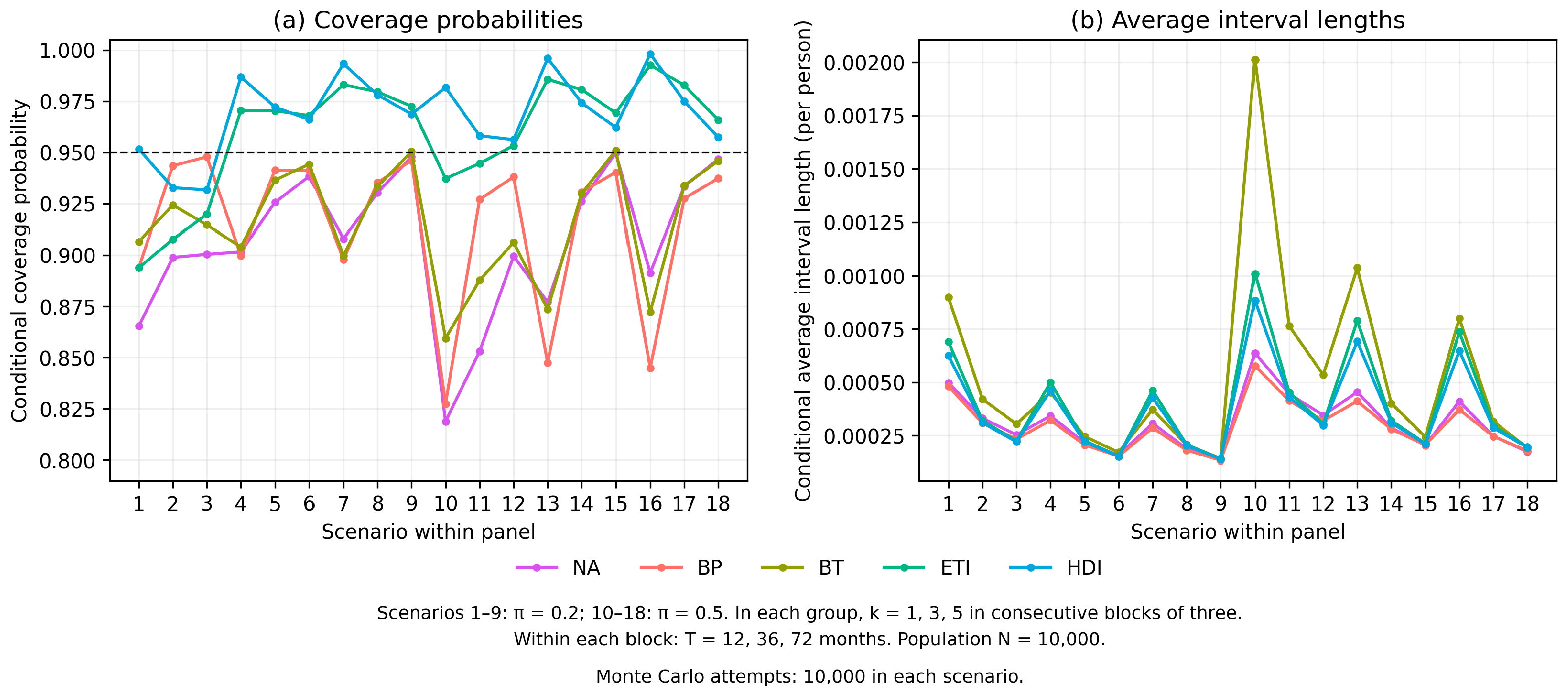
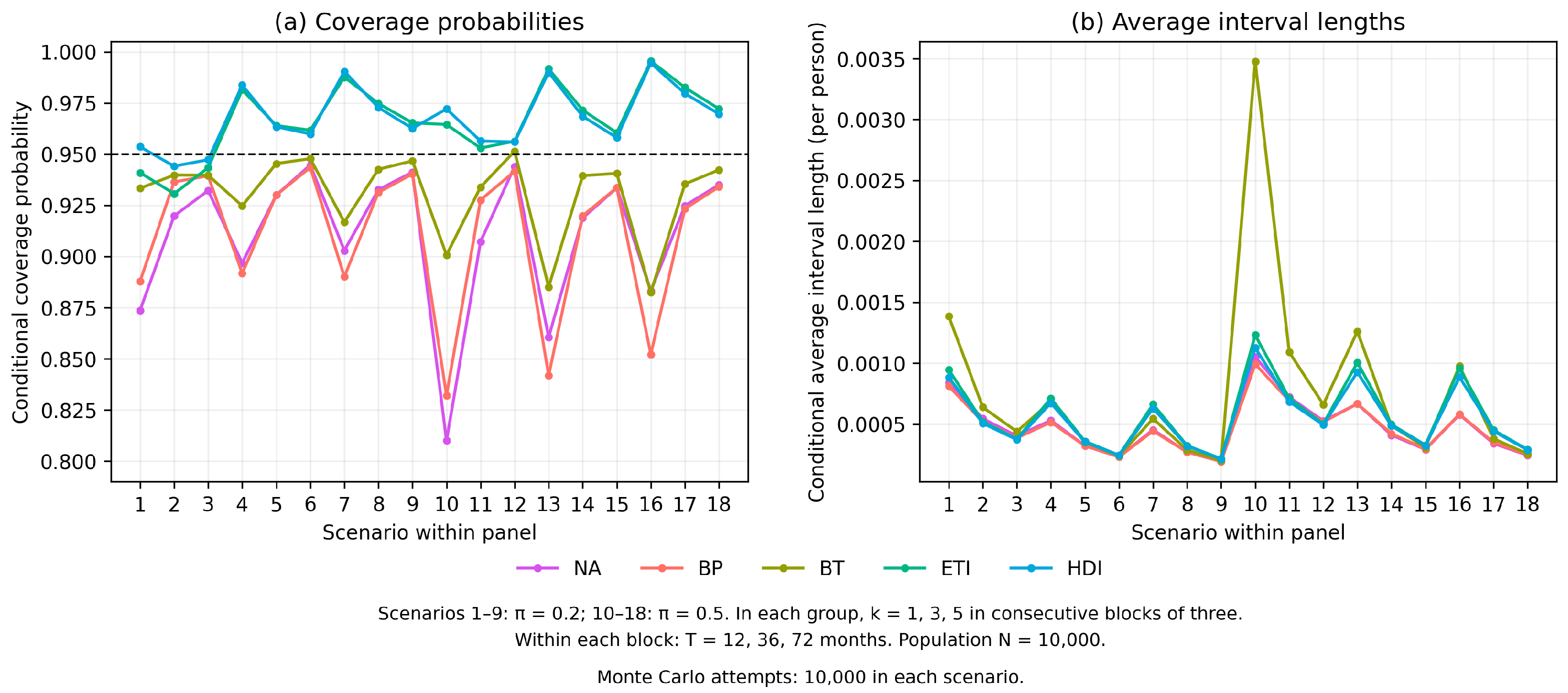
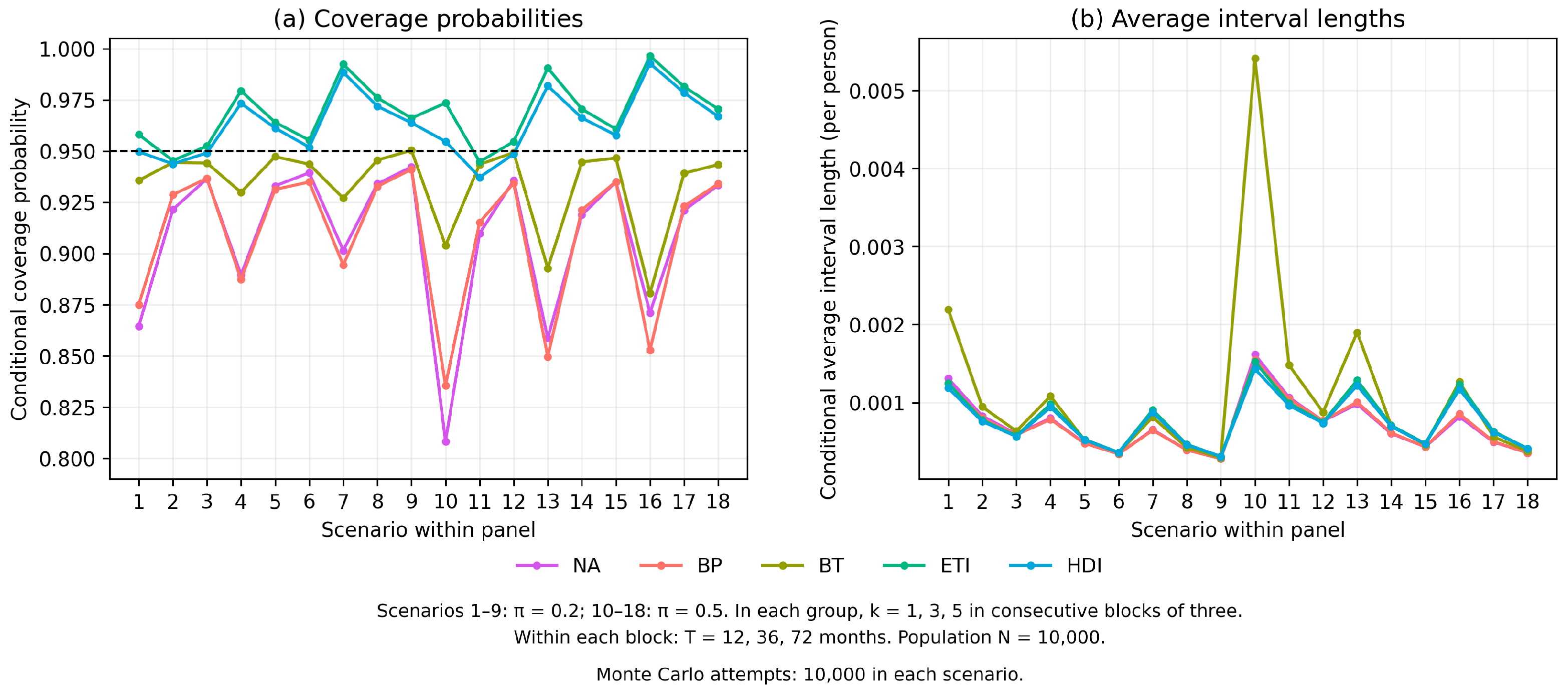
The performances of the three frequentist interval estimation methods (NA, BP, and BT) and the two Bayesian credible interval estimation methods (ETI and HDI) were compared using the coverage probability (CP) and average interval length (AL). Conditional CP was calculated as the proportion of successfully constructed intervals containing the true latent mean incidence rate. Unconditional CP used all 10,000 attempted replications per scenario as the denominator, counting failed interval construction as noncoverage. AL in Table 1 and Figure 1, Figure 2 and Figure 3 was calculated over successfully constructed intervals. Successful interval counts, failure categories, and unconditional CPs are reported in Supplementary File S1. The archived AL unconditional field equals conditional AL multiplied by the success rate; it is not an average width of valid intervals and was not used to compare interval precision. Computational efficiency was not included in the inferential comparison.

Table 1. Coverage probabilities (CPs) and average interval lengths for estimating the ZINB latent mean incidence rate with various combinations of zero-inflation probability ($\pi$), dispersion parameter (k), and exposure time (T).

Scenario	$\mathit{\pi }$	k	T	Coverage Probability (CP)					Average Interval Length
				NA	BP	BT	ETI	HDI	NA	BP	BT	ETI	HDI
Panel A: $\theta =0.0003$
1	0.2	1	12	0.8653	0.8939	0.9066	0.8939	0.9516	0.0005	0.0005	0.0009	0.0007	0.0006
2	0.2	1	36	0.8989	0.9435	0.9243	0.9077	0.9328	0.0003	0.0003	0.0004	0.0003	0.0003
3	0.2	1	72	0.9004	0.9478	0.9146	0.9198	0.9317	0.0003	0.0002	0.0003	0.0002	0.0002
4	0.2	3	12	0.9016	0.8997	0.9040	0.9705	0.9869	0.0003	0.0003	0.0005	0.0005	0.0005
5	0.2	3	36	0.9256	0.9413	0.9364	0.9704	0.9722	0.0002	0.0002	0.0002	0.0002	0.0002
6	0.2	3	72	0.9382	0.9411	0.9442	0.9680	0.9661	0.0002	0.0002	0.0002	0.0002	0.0002
7	0.2	5	12	0.9080	0.8979	0.8998	0.9831	0.9933	0.0003	0.0003	0.0004	0.0005	0.0004
8	0.2	5	36	0.9303	0.9352	0.9333	0.9796	0.9781	0.0002	0.0002	0.0002	0.0002	0.0002
9	0.2	5	72	0.9478	0.9461	0.9504	0.9725	0.9687	0.0001	0.0001	0.0001	0.0001	0.0001
10	0.5	1	12	0.8188	0.8274	0.8594	0.9372	0.9817	0.0006	0.0006	0.0020	0.0010	0.0009
11	0.5	1	36	0.8530	0.9270	0.8878	0.9446	0.9581	0.0004	0.0004	0.0008	0.0005	0.0004
12	0.5	1	72	0.8996	0.9380	0.9062	0.9533	0.9563	0.0003	0.0003	0.0005	0.0003	0.0003
13	0.5	3	12	0.8771	0.8474	0.8736	0.9857	0.9960	0.0005	0.0004	0.0010	0.0008	0.0007
14	0.5	3	36	0.9262	0.9306	0.9299	0.9807	0.9742	0.0003	0.0003	0.0004	0.0003	0.0003
15	0.5	3	72	0.9497	0.9402	0.9509	0.9693	0.9622	0.0002	0.0002	0.0002	0.0002	0.0002
16	0.5	5	12	0.8914	0.8448	0.8722	0.9927	0.9982	0.0004	0.0004	0.0008	0.0007	0.0006
17	0.5	5	36	0.9335	0.9275	0.9338	0.9828	0.9750	0.0002	0.0002	0.0003	0.0003	0.0003
18	0.5	5	72	0.9467	0.9373	0.9459	0.9659	0.9574	0.0002	0.0002	0.0002	0.0002	0.0002
Panel B: $\theta =0.0006$
1	0.2	1	12	0.8736	0.8878	0.9333	0.9410	0.9536	0.0008	0.0008	0.0014	0.0009	0.0009
2	0.2	1	36	0.9198	0.9364	0.9398	0.9307	0.9441	0.0005	0.0005	0.0006	0.0005	0.0005
3	0.2	1	72	0.9322	0.9394	0.9397	0.9434	0.9473	0.0004	0.0004	0.0004	0.0004	0.0004
4	0.2	3	12	0.8968	0.8917	0.9247	0.9814	0.9837	0.0005	0.0005	0.0007	0.0007	0.0007
5	0.2	3	36	0.9300	0.9300	0.9454	0.9640	0.9634	0.0003	0.0003	0.0003	0.0004	0.0004
6	0.2	3	72	0.9447	0.9435	0.9478	0.9617	0.9599	0.0002	0.0002	0.0002	0.0002	0.0002
7	0.2	5	12	0.9029	0.8901	0.9168	0.9877	0.9905	0.0005	0.0004	0.0005	0.0007	0.0006
8	0.2	5	36	0.9326	0.9313	0.9426	0.9748	0.9728	0.0003	0.0003	0.0003	0.0003	0.0003
9	0.2	5	72	0.9412	0.9403	0.9467	0.9653	0.9626	0.0002	0.0002	0.0002	0.0002	0.0002
10	0.5	1	12	0.8100	0.8321	0.9007	0.9645	0.9721	0.0010	0.0010	0.0035	0.0012	0.0011
11	0.5	1	36	0.9072	0.9276	0.9339	0.9530	0.9564	0.0007	0.0007	0.0011	0.0007	0.0007
12	0.5	1	72	0.9440	0.9416	0.9514	0.9563	0.9559	0.0005	0.0005	0.0007	0.0005	0.0005
13	0.5	3	12	0.8605	0.8418	0.8851	0.9917	0.9900	0.0007	0.0007	0.0013	0.0010	0.0009
14	0.5	3	36	0.9188	0.9199	0.9395	0.9715	0.9685	0.0004	0.0004	0.0005	0.0005	0.0005
15	0.5	3	72	0.9335	0.9336	0.9406	0.9605	0.9581	0.0003	0.0003	0.0003	0.0003	0.0003
16	0.5	5	12	0.8832	0.8522	0.8824	0.9955	0.9945	0.0006	0.0006	0.0010	0.0010	0.0009
17	0.5	5	36	0.9248	0.9233	0.9354	0.9826	0.9797	0.0003	0.0003	0.0004	0.0005	0.0004
18	0.5	5	72	0.9350	0.9340	0.9423	0.9722	0.9697	0.0002	0.0002	0.0003	0.0003	0.0003
Panel C: $\theta =0.001$
1	0.2	1	12	0.8644	0.8750	0.9357	0.9581	0.9497	0.0013	0.0012	0.0022	0.0012	0.0012
2	0.2	1	36	0.9215	0.9287	0.9444	0.9454	0.9438	0.0008	0.0008	0.0009	0.0008	0.0008
3	0.2	1	72	0.9365	0.9367	0.9442	0.9524	0.9491	0.0006	0.0006	0.0006	0.0006	0.0006
4	0.2	3	12	0.8897	0.8873	0.9299	0.9794	0.9733	0.0008	0.0008	0.0011	0.0010	0.0009
5	0.2	3	36	0.9330	0.9313	0.9473	0.9641	0.9613	0.0005	0.0005	0.0005	0.0005	0.0005
6	0.2	3	72	0.9394	0.9349	0.9436	0.9553	0.9519	0.0003	0.0003	0.0004	0.0004	0.0004
7	0.2	5	12	0.9015	0.8943	0.9270	0.9924	0.9885	0.0007	0.0006	0.0008	0.0009	0.0009
8	0.2	5	36	0.9340	0.9327	0.9456	0.9760	0.9719	0.0004	0.0004	0.0004	0.0005	0.0005
9	0.2	5	72	0.9423	0.9411	0.9504	0.9661	0.9638	0.0003	0.0003	0.0003	0.0003	0.0003
10	0.5	1	12	0.8082	0.8356	0.9039	0.9735	0.9547	0.0016	0.0016	0.0054	0.0015	0.0014
11	0.5	1	36	0.9098	0.9152	0.9435	0.9448	0.9372	0.0011	0.0010	0.0015	0.0010	0.0010
12	0.5	1	72	0.9356	0.9343	0.9493	0.9546	0.9485	0.0008	0.0008	0.0009	0.0007	0.0007
13	0.5	3	12	0.8585	0.8496	0.8928	0.9906	0.9819	0.0010	0.0010	0.0019	0.0013	0.0012
14	0.5	3	36	0.9188	0.9213	0.9447	0.9705	0.9662	0.0006	0.0006	0.0007	0.0007	0.0007
15	0.5	3	72	0.9350	0.9351	0.9466	0.9608	0.9577	0.0004	0.0004	0.0005	0.0005	0.0005
16	0.5	5	12	0.8710	0.8528	0.8806	0.9965	0.9928	0.0008	0.0009	0.0013	0.0012	0.0012
17	0.5	5	36	0.9211	0.9231	0.9392	0.9815	0.9785	0.0005	0.0005	0.0006	0.0006	0.0006
18	0.5	5	72	0.9333	0.9340	0.9434	0.9705	0.9669	0.0004	0.0004	0.0004	0.0004	0.0004

Note: CP and AL are conditional on successful interval construction. T is measured in months; N = 10,000 denotes population exposure. Values are rounded to four decimal places for consistency with the original table; the CSV and figures retain full numeric precision. Scenario numbering restarts within each panel. Each scenario comprised 10,000 Monte Carlo attempts. Counts of successful intervals, unconditional CPs, failure categories, and all-zero datasets are available in Supplementary File S1.

Figure 1. Performance comparison of the interval estimation methods for the ZINB latent mean incidence rate when $\theta =0.0003$.

Figure 2. Performance comparison of the interval estimation methods for the ZINB latent mean incidence rate when $\theta =0.0006$.

Figure 3. Performance comparison of interval estimation methods for the ZINB latent mean incidence rate when $\theta =0.001$.

All statistical analyses were performed using Python (version 3.14.4 for simulations and version 3.14.7 for empirical analyses). The simulation used NumPy (version 2.5.3) and PyTorch (version 2.14.0) for numerical computation, a custom HMC sampler implemented with PyTorch for Bayesian inference, and ArviZ (version 0.22.0) for posterior diagnostics. The empirical frequentist analyses used SciPy (version 1.18.1), whereas empirical Bayesian inference used the No-U-Turn Sampler (NUTS) implemented in Stan (version 2.40.0) through CmdStanPy (version 1.3.0). Data processing and graphical presentation used pandas (version 3.0.6) and Matplotlib (version 3.11.2), respectively. The simulation used a base random seed of 20260929. The Monte Carlo simulation procedure is summarized in Algorithm 5.

Algorithm 5  Monte Carlo Simulation Procedure

1:  Specify the simulation parameters, including the latent mean incidence rate (θ), zero-inflation probability (π), dispersion parameter (k), observation period (T), and population at risk (N). 2:  Generate one dataset from the ZINB model according to the data-generating mechanism described in Section 2.2. 3:  Estimate the model parameters using the procedure described in Section 2.3. 4:  Construct interval estimates using the five competing methods (NA, BP, BT, ETI, and HDI). 5:  Record interval-construction success or failure separately for each method. For each successful interval, record whether it contains the true latent mean incidence rate and calculate its length. Record all-zero datasets and available fit and sampling diagnostics. 6:  Repeat Steps 2–5 for all Monte Carlo replications. 7:  Repeat the entire simulation procedure for all combinations of $\theta ,\pi ,k$ and T. 8:  Summarize the performance of each method using conditional CP and AL, unconditional CP, and interval-construction success and failure counts.

3. Results

3.1. Simulation Study

Table 1 summarizes the simulation results, which are grouped into three panels according to the latent mean incidence rate: Panel A $(\theta =0.0003)$, Panel B $(\theta =0.0006)$, and Panel C $(\theta =0.001)$, while Figure 1, Figure 2 and Figure 3 present graphical comparisons of the coverage probabilities and average lengths for the five competing methods. The CPs and ALs in Table 1 and Figure 1, Figure 2 and Figure 3 are conditional on successful interval construction. Successful interval counts, unconditional CPs, all-zero counts, and diagnostic summaries are provided in Supplementary File S1. Bayesian intervals often had higher conditional coverage than the frequentist intervals, but they did not consistently lie closest to 0.95. The BT method had the smallest absolute deviation from 0.95 in 23 of 54 scenarios compared with 13 for HDI, 11 for ETI, 5 for BP, and 2 for NA. These descriptive rankings do not establish statistically significant differences between methods.

As can be seen in Panel A in Table 1 and Figure 1, the smallest incidence rate setting ($\theta =0.0003$) showed substantial variation in coverage. Under severe zero inflation ($\pi =0.5$), $k=1$, and $T=12$, conditional CPs were 0.8188, 0.8274, 0.8594, 0.9372, and 0.9817 for NA, BP, BT, ETI, and HDI, respectively. In this setting, ETI was closer to nominal coverage than HDI. BT had higher conditional coverage than BP in 11 of the 18 Panel A scenarios. In terms of interval precision, Figure 1 shows that BP and NA generally produced shorter intervals, although HDI was shortest in selected scenarios. At $\pi =0.5$, $k=1$, and $T=12$, BT had an average length of 0.0020 compared with 0.0006 for BP. HDI was shorter than ETI in every Panel A scenario.

A similar pattern can be observed for $\theta =0.0006$ (Panel B in Table 1). Conditional coverage ranged from 0.8100 to 0.9447 for NA, 0.8321 to 0.9435 for BP, 0.8824 to 0.9514 for BT, 0.9307 to 0.9955 for ETI, and 0.9441 to 0.9945 for HDI. BT exceeded BP in 16 of 18 scenarios. Increasing the observation period generally improved frequentist coverage and reduced average lengths, although Bayesian coverage did not improve monotonically toward 0.95. At $\pi =0.5$, $k=1$, and $T=12$, the BT average length was 0.0035 compared with 0.0010 for BP. Figure 2 therefore shows improved BT coverage accompanied by substantially wider intervals in some short-series settings.

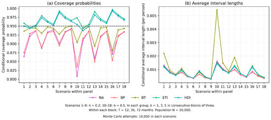
For the largest incidence rate setting ($\theta =0.001$), the results provided in Panel C in Table 1 and Figure 3 show the same coverage–length trade-off. Conditional CPs ranged from 0.8082 to 0.9423 for NA, 0.8356 to 0.9411 for BP, and 0.8806 to 0.9504 for BT. BT exceeded BP in all 18 scenarios, but its average lengths were greater in every scenario. At $\pi =0.5$, $k=1$, and $T=12$, the BT average length was 0.0054 compared with 0.0016 for BP. Bayesian conditional coverage ranged from 0.9448 to 0.9965 for ETI and 0.9372 to 0.9928 for HDI, showing both undercoverage and overcoverage.

Several consistent patterns were observed across all three panels of Table 1. Increasing the observation period generally reduced average lengths and improved frequentist coverage. NA and BP had conditional CPs below 0.95 in every scenario, whereas BT exceeded BP in 47 of 54 scenarios and attained conditional CPs above 0.95 in four scenarios. ETI and HDI had conditional CPs above 0.95 in 44 and 45 scenarios, respectively; HDI was shorter than ETI in all 54 scenarios. Thus, higher coverage did not necessarily imply closer calibration to the nominal level, and NA did not uniformly provide the shortest intervals. Counting interval-construction failures changed the comparison materially. For example, at $\theta =0.001$, $\pi =0.5$, $k=1$, and $T=36$, 8472 of 10,000 Bayesian intervals were accepted. ETI conditional and unconditional CPs were 0.9448 and 0.8004, while the corresponding HDI values were 0.9372 and 0.7940. BT constructed 9998 intervals with conditional and unconditional CPs of 0.9435 and 0.9433. Thus, failures should be considered alongside CP and AL.

Overall, no method uniformly achieved nominal coverage across the evaluated ZINB scenarios. BT often improved coverage relative to NA and BP, but its interval lengths could be substantially greater. Bayesian intervals frequently had high conditional coverage, and HDI was consistently shorter than ETI, but overcoverage and diagnostic-related failures limited claims of general superiority. Across scenarios, failures ranged from 0 to 211 for NA, 0 to 83 for BP, 0 to 504 for BT, and 0 to 1528 for each Bayesian method. These findings demonstrate the importance of considering interval precision, calibration, and construction success jointly under the specified main prior.

A separate auxiliary prior-sensitivity analysis was conducted for six representative scenarios using the corrected multi-chain HMC implementation. The same datasets were evaluated under the Gamma(2, 2000) prior used in the main simulation, a weakly informative lognormal prior with $\log \left(\theta \right)\sim \mathrm{Normal}\left(\log \left(0.001\right),2^2\right)$, and a deliberately misspecified Gamma(20, 2000) prior for $\theta$; nuisance-parameter priors were held fixed. Conditional CP under the main and weak priors ranged from 0.9220 to 0.9990 and from 0.9488 to 0.9960, respectively, across ETI and HDI. These results were broadly comparable but did not demonstrate nominal coverage in every scenario. Under the misspecified prior, conditional CP ranged from 0 to 0.7906, and interval-construction success ranged from 47.0% to 99.8%. The substantial diagnostic failures under this prior limit the interpretation of conditional coverage and prevent the attribution of unconditional undercoverage solely to prior specification. Results, diagnostics, code, simulation settings, and replication counts are provided in Supplementary File S2. This auxiliary analysis was not used to construct Table 1.

3.2. Empirical Study

This was carried out using secondary dengue surveillance data from the Provincial Public Health Office in Phayao Province, Thailand, from January 2017 to December 2024. The dataset consisted of 864 observations, each providing the monthly number of reported dengue fever cases within each district in the province, as well as the corresponding population therein at risk. These observations comprised 96 months of data from each of the nine districts. Ethical approval for this study was obtained from the Human Research Ethics Committee of University of Phayao, Thailand (Approval No. HREC-UP-HSST 1.1/068/68). Since the analysis was based on anonymized secondary surveillance data, informed consent from individual participants was not required. Therefore, the observed incidence rate was computed as

$$R_{ij}={\displaystyle \frac{Y_{ij}}{N_{ij}}},$$

where $Y_{ij}$ denotes the number of reported dengue cases and $N_{ij}$ denotes the population at risk for district i during month j. Following the framework proposed in Section 2.2, the empirical analysis focused on the overall provincial incidence pattern rather than district-specific inference.

Preliminary descriptive analysis showed a mean monthly number of dengue cases of 3.9896, whereas the variance was 98.6708, yielding a variance-to-mean ratio of 24.7321. In addition, 53.36% of the observations were zero counts with a median of zero. These results indicate substantial overdispersion together with a high proportion of zero observations. Such patterns suggest that the Poisson assumption of equal mean and variance is inadequate and that more flexible count-data models should be considered.

To accommodate these distributional characteristics, Poisson, NB, zero-inflated Poisson (ZIP), and ZINB models were fitted to the dengue surveillance data, and their goodness of fit was compared using the log-likelihood, AIC, and BIC (Table 2). The NB and ZINB models performed significantly better than the Poisson and ZIP models and generated almost identical log-likelihood values, indicating that both models provided comparable fits to the dengue surveillance data. Furthermore, both models closely reproduced the observed proportion of zero counts, whereas the Poisson model substantially underestimated the frequency of zeros. Although the NB model yielded the smallest AIC and BIC values, the differences from the ZINB model were small. Because the primary objective of this study was to evaluate interval estimation methods under the ZINB framework, the fitted ZINB model was retained for the subsequent empirical illustration.

Table 2. Comparison of Poisson, NB, ZIP, and ZINB models fitted to the dengue surveillance data.

Model	Log-Likelihood	AIC	BIC	Akaike Weight	Predicted Zero Proportion
Poisson	−5244.0734	10,490.1468	10,494.9084	0.0000	0.0704
NB	−1741.2427	3486.4855	3496.0086	0.7311	0.5396
ZIP	−3627.1984	7258.3967	7267.9199	0.0000	0.5320
ZINB	−1741.2427	3488.4855	3502.7702	0.2689	0.5396

Note: The observed proportion of zero counts was 0.5336. An exploratory likelihood-ratio comparison between the NB and ZINB models indicated negligible improvement after introducing the zero-inflation component. Although the NB model achieved slightly lower AIC and BIC values, the ZINB model was retained because it constitutes the methodological framework investigated in this study.

The estimated zero-inflation probability from the fitted ZINB model was approximately $1.13\times {10}^{-7}$ at its lower numerical bound. This finding is consistent with the exploratory likelihood-ratio comparison between the NB and ZINB models, suggesting that the excess of zero counts in the data can be well explained by overdispersion described by the negative binomial component without a separate structural-zero process. For the empirical NA and BT intervals, the standard error of $\theta$ was calculated from the local curvature of the observed negative-log-likelihood Hessian with free nuisance parameters eliminated by a Schur complement and nuisance parameters on a numerical bound held fixed. The same calculation was performed for each accepted bootstrap replicate used in BT. BP required an accepted point fit, whereas BT additionally required a finite positive standard error. The Bayesian posterior mean for the latent mean incidence rate under the fitted ZINB model was 1.4794, whereas the frequentist estimate was 1.3573 (Table 3). Both estimates are reported as cases per 10,000 persons. In the empirical code, $\theta$ and its Gamma(2, 2000) prior are specified on the per-person scale; the estimates and interval endpoints are multiplied by 10,000 only for presentation. The two estimates are in close agreement, indicating that the frequentist and Bayesian methods produce similar estimates for the latent mean incidence rate. The empirical Bayesian analysis used four Stan NUTS chains, with 1500 warm-up iterations and 2000 retained draws per chain, adapt_delta = 0.95, and max_treedepth = 12. Across $\theta$, $\pi$, and k, the maximum $\widehat{R}$ was 1.0009, the minimum bulk ESS was 2262.1, and the minimum tail ESS was 2882.7 with no divergences or tree-depth limit.

Table 3. Frequentist and Bayesian estimates together with 95% interval estimates for the latent mean incidence rate under the fitted ZINB model.

Panel A. Parameter estimates
Parameter	Frequentistestimate		Bayesianposterior mean
Latent mean incidence rate, $\theta$	1.3573		1.4794
Zero-inflation probability, $\pi$	0.0000		0.0683
Dispersion parameter, k	0.2221		0.2487
Panel B. Interval estimates for $\mathit{\theta }$
Method	Lower limit	Upper limit	Interval length
NA	1.1578	1.5569	0.3991
BP	1.1298	1.6290	0.4992
BT	1.1351	1.6442	0.5091
Bayesian ETI	1.2510	1.7523	0.5014
Bayesian HDI	1.2345	1.7274	0.4929

Note: The latent incidence rate and its interval endpoints are reported per 10,000 persons; $\pi$ and k are dimensionless. The intervals use a pooled independent ZINB likelihood. Temporal-dependence and bootstrap-replication sensitivity analyses are reported under ‘Temporal dependence and sensitivity analyses’ below and Supplementary Files S3 and S4.

Table 3 summarizes the frequentist and Bayesian parameter estimates together with the corresponding 95% interval estimates for the latent mean incidence rate. Among the five interval estimation methods, the NA produced the narrowest interval, whereas the BP and BT methods resulted in relatively wider intervals. The ETI and HDI produced highly similar credible intervals with the HDI being marginally shorter than the ETI. Overall, the empirical analysis illustrates the five interval procedures under a fitted ZINB model. Because the NB model had lower AIC and BIC and the fitted zero-inflation probability was near zero, these data do not independently validate interval performance under structural zero inflation.

3.3. Temporal Dependence and Sensitivity Analyses

District-specific autocorrelation functions (ACFs) were examined for monthly case counts and Pearson residuals from the pooled ZINB model. Exploratory Ljung–Box tests at lags 6 and 12 were adjusted using the Holm procedure across 18 district–lag tests separately for counts and residuals. These tests were treated as approximate diagnostics because the observations were discrete, the residuals were calculated from a fitted model, and the series could be nonstationary. Synchronized noncircular moving-block bootstrap samples were generated using 3-, 6-, and 12-month blocks, selecting the same months across all nine districts and retaining count–population pairs. BP intervals were calculated from the resulting estimates. Bootstrap sensitivity was assessed at $B=500$, 1000, 2000, and 5000 attempts for BP and BT based on an independent resampling of observation pairs (iid bootstrap) and for BP based on block resampling. Within each resampling scheme, the analysis at each B used the first B attempts from the same bootstrap sequence. Procedures, seeds, and fit audits are provided in Supplementary Files S3 and S4.

Pearson residual lag-1 autocorrelations ranged from 0.2439 to 0.8301. Holm-adjusted Ljung–Box tests indicated residual temporal dependence in eight of nine districts at both lags 6 and 12 with Phu Kamyao the exception; case-count diagnostics showed similar patterns. At $B=1000$, BP interval lengths for 3-, 6-, and 12-month blocks were 1.2827, 1.6373, and 1.7662, respectively, compared with 0.4992 for iid BP, which were all expressed per $\mathrm{10,000}$ persons. Relative to $B=1000$, increasing B to 5000 changed interval lengths by $-2.66\%$ to $+3.33\%$ across the five method–resampling combinations. All 5000 point fits were accepted in each resampling scheme, and all iid BT replicates had finite positive standard errors. At least one parameter was on a numerical bound in 4991 iid replicates and in 4788, 4822, and 4858 replicates for 3-, 6-, and 12-month blocks, respectively. Full results are reported in Supplementary Tables S1–S4.

The ZINB intervals in Table 3 illustrate latent rate estimation under the fitted pooled independent model and should not be interpreted as accounting for serial dependence. Block BP intervals were substantially wider than iid BP intervals, indicating sensitivity to the resampling scheme. These exploratory results do not establish nominal coverage, and a single nested bootstrap sequence does not establish endpoint convergence or quantify variability across independent seeds. Seasonality, nonstationarity, and frequent boundary fits may affect interval calibration. Likewise, satisfactory Bayesian sampling diagnostics do not validate the independence assumption.

4. Discussion and Conclusions

This study compared frequentist and Bayesian interval estimation methods for the ZINB latent mean incidence rate. The simulation results showed that interval estimation performance depended strongly on the degree of zero inflation, the dispersion parameter, and the observation period. Bayesian approaches often achieved higher conditional coverage than the frequentist methods, but overcoverage meant that they were not consistently closest to the nominal level. BT was closest to 0.95 in more scenarios than either Bayesian method individually. Conversely, NA showed substantial undercoverage when zero inflation was high and k was small, although it did not uniformly provide the shortest intervals. A shorter interval does not necessarily lead to more reliable inference when the nominal coverage has not been achieved. These results emphasize the trade-off between interval precision and statistical calibration.

The BP and BT intervals generally provided better coverage performance than the NA method, but both bootstrap approaches remained sensitive to short observation periods and strong zero inflation. BT achieved higher conditional coverage than BP in 47 of 54 scenarios, although this improvement was accompanied by wider interval lengths. HDI was shorter than ETI in all 54 scenarios, while both Bayesian methods often showed overcoverage under the main prior. Their unconditional coverage was substantially lower in scenarios with frequent diagnostic-related failures. Collectively, these results support considering Bayesian credible intervals as alternatives to frequentist intervals while limiting any advantage to the evaluated scenario, prior, and interval-construction protocol. Successful computation and high conditional coverage alone do not establish uniform inferential reliability.

The empirical application to the dengue surveillance data of Phayao Province illustrated the interval procedures under the fitted ZINB model. Model comparison showed that the NB and ZINB models substantially outperformed the Poisson and ZIP models, confirming that accounting for overdispersion is essential for adequately describing dengue surveillance data. Although the estimated zero-inflation probability under the fitted ZINB model was close to zero, this finding was consistent with the likelihood-based comparison between the NB and ZINB models and suggests that much of the observed excess zeros could be explained by overdispersion accommodated through the negative binomial component rather than by a distinct structural-zero process. Nevertheless, the ZINB model was retained because it represents the inferential framework investigated in this study. Under the fitted model, the Bayesian and frequentist approaches produced comparable point estimates of the latent mean incidence rate, whereas the Bayesian ETI and HDI yielded similar credible intervals. Because the NB model fitted at least as well as the ZINB model and the estimated zero-inflation probability was near zero, this application should be interpreted as an illustration of the interval procedures rather than confirmation of their performance under structural zero inflation. Temporal diagnostics indicated residual dependence in eight of nine districts, and synchronized block BP intervals were substantially wider than iid BP intervals. Increasing bootstrap attempts from 1000 to 5000 changed interval lengths by $-2.66\%$ to $+3.33\%$ without changing this qualitative finding. These results highlight sensitivity to dependence assumptions; they do not validate nominal coverage or establish the superiority of an interval method.

In conclusion, the simulation results under the specified main prior do not identify a uniformly best interval estimator for the ZINB latent mean incidence rate. BT generally improved coverage relative to BP but could produce substantially longer intervals. HDI was consistently shorter than ETI, while Bayesian overcoverage and diagnostic-related failures qualified its advantages. Although the fitted dengue surveillance data could also be adequately described by the NB model, the ZINB framework offers a flexible framework for evaluating interval estimation methods applicable to sparse, overdispersed, and potentially zero-inflated surveillance data. The empirical application illustrates the methods without establishing a structural-zero component in these data. Future research may extend the framework to hierarchical, longitudinal, and spatiotemporal count models; extend prior-sensitivity analyses to additional scenarios and prior specifications; examine simulation sensitivity to bootstrap and posterior sample size; and compare additional performance measures, including interval scores.

References

- Cameron, A.C.; Trivedi, P.K. Regression Analysis of Count Data, 2nd ed.; Cambridge University Press: Cambridge, UK, 2013. [Google Scholar]
- Fraser, G.E. The estimation of disease frequency using a population sample. Int. J. Epidemiol. 1978, 7, 277–284. [Google Scholar] [CrossRef] [Scilit] [PubMed]
- Noordzij, M.; Dekker, F.W.; Zoccali, C.; Jager, K.J. Measures of Disease Frequency: Prevalence and Incidence. Nephron Clin. Pract. 2010, 115, c17–c20. [Google Scholar] [CrossRef] [Scilit] [PubMed]
- Lee, J.; Han, G.; Fulp, W.J.; Giuliano, A.R. Analysis of overdispersed count data: Application to the Human Papillomavirus Infection in Men (HIM) Study. Epidemiol. Infect. 2012, 140, 1087–1094. [Google Scholar] [CrossRef] [Scilit] [PubMed]
- Roosa, K.; Luo, R.; Chowell, G. Comparative assessment of parameter estimation methods in the presence of overdispersion: A simulation study. Math. Biosci. Eng. 2019, 16, 4299–4313. [Google Scholar] [CrossRef] [Scilit] [PubMed]
- Angelakis, A.; Nyawanda, B.O.; Vounatsou, P. Modeling sparse Rift Valley fever incidence data: A Bayesian perspective on zero-inflated self-exciting and autoregressive models. BMC Infect. Dis. 2025, 25, 1221. [Google Scholar] [CrossRef] [Scilit] [PubMed]
- Feng, C.X. A comparison of zero-inflated and hurdle models for modeling zero-inflated count data. J. Stat. Distrib. Appl. 2021, 8, 8. [Google Scholar] [CrossRef] [Scilit] [PubMed]
- Hilbe, J.M. Negative Binomial Regression, 2nd ed.; Cambridge University Press: Cambridge, UK, 2011. [Google Scholar]
- Lambert, D. Zero-Inflated Poisson Regression, with an Application to Defects in Manufacturing. Technometrics 1992, 34, 1–14. [Google Scholar] [CrossRef] [Scilit]
- Perumean-Chaney, S.E.; Morgan, C.; McDowall, D.; Aban, I. Zero-inflated and overdispersed: What’s one to do? J. Stat. Comput. Simul. 2013, 83, 1671–1683. [Google Scholar] [CrossRef] [Scilit]
- Hwang, W.; Chen, L.; Stoklosa, J. Counting the Unseen: Estimation of Susceptibility Proportions in Zero-Inflated Models Using a Conditional Likelihood Approach. Am. Stat. 2024, 78, 161–170. [Google Scholar] [CrossRef] [Scilit]
- Moghimbeigi, A.; Eshraghian, M.R.; Mohammad, K.; McArdle, B. Multilevel zero-inflated negative binomial regression modeling for over-dispersed count data with extra zeros. J. Appl. Stat. 2008, 35, 1193–1202. [Google Scholar] [CrossRef] [Scilit]
- Workie, M.S.; Yi, X. Robust Bayesian Inference in the Multilevel Zero-Inflated Generalized Poisson Model. Stat. Med. 2025, 44, e70173. [Google Scholar] [CrossRef] [Scilit] [PubMed]
- Khurshid, A.; Ageel, M.; Lodhi, R. On Confidence Intervals for the Negative Binomial Distribution. Investig. Oper. 2005, 26, 59–70. [Google Scholar]
- Hasan, M.; Krishnamoorthy, K. Confidence Intervals and Prediction Intervals for Two-Parameter Negative Binomial Distributions. J. Appl. Stat. 2023, 51, 2420–2435. [Google Scholar] [CrossRef] [Scilit] [PubMed]
- Doi, J.; Holladay, B.; Schilling, M. Improved Interval Estimation of Negative Binomial Parameters: A Coverage Probability Approach. J. Stat. Comput. Simul. 2023, 94, 126–141. [Google Scholar] [CrossRef] [Scilit]
- Holladay, B.; Schilling, M. Short Confidence Intervals for the Count Parameters of the Binomial, Negative Binomial, and Hypergeometric Distributions. Commun. Stat. Theory Methods 2024, 54, 5428–5442. [Google Scholar] [CrossRef] [Scilit]
- Saha, K.; Paul, S. Interval Estimation of the Negative Binomial Dispersion Parameter. J. Stat. Comput. Simul. 2011, 81, 1993–2002. [Google Scholar] [CrossRef] [Scilit]
- Gelman, A.; Carlin, J.B.; Stern, H.S.; Dunson, D.B.; Vehtari, A.; Rubin, D.B. Bayesian Data Analysis, 3rd ed.; CRC Press: Boca Raton, FL, USA, 2014. [Google Scholar]
- Kelter, R. The evidence interval and the Bayesian evidence value: On a unified theory for Bayesian hypothesis testing and interval estimation. Br. J. Math. Stat. Psychol. 2022, 75, 550–592. [Google Scholar] [CrossRef] [Scilit] [PubMed]
- Hall, D.B. Zero-inflated Poisson and binomial regression with random effects. Biometrics 2000, 56, 1030–1039. [Google Scholar] [CrossRef] [Scilit] [PubMed]
- Khandeparkar, P.; Sabnis, S. Simultaneous Confidence Intervals for Parameters of Zero-Inflated Negative Binomial Model and Hurdle Negative Binomial Model. J. Stat. Theory Pract. 2025, 20, 264–278. [Google Scholar] [CrossRef] [Scilit]
- Hu, C.; Fang, L.; Shi, X.; Wang, Y. Bayesian Inference for Zero-Inflated Negative Binomial Lindley Model of Overdispersed Count Data with Excess Zeros. Int. J. Ind. Eng. Comput. 2025, 16, 1077–1088. [Google Scholar] [CrossRef] [Scilit]
- Efron, B.; Tibshirani, R.J. An Introduction to the Bootstrap; Chapman & Hall: London, UK, 1993. [Google Scholar]
- Davison, A.C.; Hinkley, D.V. Bootstrap Methods and Their Application; Cambridge University Press: Cambridge, UK, 1997. [Google Scholar]
- DiCiccio, T.J.; Romano, J.P. A Review of Bootstrap Confidence Intervals. J. R. Stat. Soc. Ser. B 1988, 50, 338–354. [Google Scholar] [CrossRef] [Scilit]
- Puth, M.; Neuhauser, M.; Ruxton, G.D. On the variety of methods for calculating confidence intervals by bootstrapping. J. Anim. Ecol. 2015, 84, 892–897. [Google Scholar] [CrossRef] [Scilit] [PubMed]
- Carpenter, J.; Bithell, J. Bootstrap confidence intervals: When, which, what? A practical guide for medical statisticians. Stat. Med. 2000, 19, 1141–1164. [Google Scholar] [CrossRef] [Scilit]
- Davidian, M.; Carroll, R.J. Variance Function Estimation. J. Am. Stat. Assoc. 1987, 82, 1079–1091. [Google Scholar] [CrossRef]
- Efron, B. Better bootstrap confidence intervals. J. Am. Stat. Assoc. 1987, 82, 171–185. [Google Scholar] [CrossRef] [Scilit]
- van der Vaart, A.W. Asymptotic Statistics; Cambridge University Press: Cambridge, UK, 1998. [Google Scholar]
- Janas, D. A Smoothed Bootstrap Estimator for a Studentized Sample Quantile. Ann. Inst. Stat. Math. 1993, 45, 317–329. [Google Scholar] [CrossRef] [Scilit]
- Angelis, D.D.; Hall, P.; Young, G.A. A Note on Coverage Error of Bootstrap Confidence Intervals for Quantiles. Math. Proc. Camb. Philos. Soc. 1993, 114, 517–531. [Google Scholar] [CrossRef] [Scilit]
- Ho, Y.H.S.; Lee, S.M.S. Iterated Smoothed Bootstrap Confidence Intervals for Population Quantiles. Ann. Stat. 2005, 33, 437–462. [Google Scholar] [CrossRef] [Scilit]
Disclaimer/Publisher’s Note: The statements, opinions and data contained in all publications are solely those of the individual author(s) and contributor(s) and not of MDPI and/or the editor(s). MDPI and/or the editor(s) disclaim responsibility for any injury to people or property resulting from any ideas, methods, instructions or products referred to in the content. |
© 2026 by the authors. Licensee MDPI, Basel, Switzerland. This article is an open access article distributed under the terms and conditions of the Creative Commons Attribution (CC BY) license.