Fractional Symmetry and Comparison Structures of the Lerch Transcendent

Abstract

The Lerch transcendent is a three-parameter special function containing the Riemann zeta, Hurwitz zeta, Dirichlet eta, and polylogarithm functions as distinguished specializations. This study develops a defect-based framework for comparing fractional differentiation with parameter transformations and authentic functional covariances of Lerch-type functions. The fractional operator is fixed throughout as the right Weyl–Marchaud derivative in the spectral variable. First, this study separates arbitrary comparison pullbacks from genuine weighted covariance operators and establish explicit conditions under which the Lerch series may be differentiated termwise, including an integrable tail estimate that justifies interchange with the unbounded Weyl integral in the regimes used in the paper. Then, the full commutator of the fractional derivative with a weighted composition operator is analyzed, including the pullback contribution. Beyond the general formalism, the Hurwitz zeta duplication formula is studied as a concrete non-elementary covariance. Its fractional symmetry defect is obtained both as a convergent Marchaud integral and as an explicit Dirichlet series. For $0<\alpha <1$, $a>2$, and real $s>1$, this defect is strictly positive, showing that the classical duplication covariance is not preserved by the chosen fractional operator in that region. The geometrically forced fixed-point line used in the comparison examples and the numerical experiments is retained as a calibration benchmark rather than as evidence for a shifted critical strip. A concrete spectral-zeta realization is also provided for the affine-spectrum operator whose spectral zeta function is the Hurwitz zeta function.

1. Introduction

Symmetry is a central organizing principle in mathematical analysis. For special functions, it often appears through reflection formulas, functional equations, conjugation laws, translation identities, and transformations of parameters. Such relations are not merely formal: they connect values in distinct regions of the complex plane, constrain zero sets, guide analytic continuation, and provide efficient numerical representations. The Riemann zeta functional equation is the best-known example, but it belongs to a broader network of identities involving the Hurwitz zeta function, periodic zeta functions, polylogarithms, Dirichlet series, and the Lerch transcendent [1,2,3,4].

The Lerch transcendent is defined by [2,5,6]

$$\Phi (z,s,a)={\displaystyle \sum _{n=0}^{\infty }}{\displaystyle \frac{z^n}{{(n+a)}^s}}$$

(1)

in a domain where the series converges and where the chosen branch of the power is well defined. For $\left|z\right|<1$, the series converges absolutely for every $s\in \mathbb{C}$ (away from the excluded values of a). If $\left|z\right|=1$, absolute convergence requires $\mathrm{Re}\left(s\right)>1$; when $\left|z\right|=1$ and $z\ne 1$, conditional convergence extends to $\mathrm{Re}\left(s\right)>0$ by Dirichlet–Abel summation under the standard branch restrictions on a. Analytic continuation extends the function well beyond the disk of absolute convergence [6,7,8]. The three variables play distinct roles: z determines the geometric weight, s is the spectral exponent, and a shifts the underlying lattice. Consequently, the Lerch transcendent provides a unified framework containing the Riemann zeta function, the Hurwitz zeta function, the Dirichlet eta function, and the polylogarithm as special cases.

Fractional calculus extends differentiation and integration to non-integer orders and has become an important tool in the analysis of nonlocal phenomena [9,10,11,12]. In the complex plane, however, fractional differentiation is not unique: different operators, branch conventions, and differentiation directions lead to different analytical properties [13,14]. This operator dependence becomes particularly relevant for special functions and motivates the present investigation.

Several authors have investigated fractional derivatives of the Riemann, Hurwitz, and Lerch zeta functions, deriving fractional representations and related analytic formulas [15,16,17,18]. These developments motivate the present study, but they also make the choice of fractional operator mathematically decisive. Accordingly, this paper fixes one operator from the outset and does not infer a universal displacement of the classical critical strip from the fractional order. For the Weyl–Marchaud operator adopted below, fractional differentiation of the Dirichlet modes introduces logarithmic weights; such weights do not change the abscissa of absolute convergence of the Riemann/Hurwitz Dirichlet series. The purpose of the paper is therefore more specific: to quantify the failure (or preservation) of covariance when a fractionally differentiated Lerch-type function is compared with a parameter-transformed value. We distinguish an arbitrary comparison transformation from a genuine classical symmetry. In the latter case, the functional equation, including any multiplicative factor, is encoded in a weighted symmetry operator and the fractional defect is a commutator. We use the term critical structure only as an umbrella description for analytically distinguished sets; convergence boundaries, fixed-point sets, defect-zero sets, stationary sets, and threshold sets are defined separately and are not assumed to coincide. In this paper, the term fractional symmetry and comparison structures is used as a collective designation for the objects generated by these two distinct constructions. Genuine symmetry structures arise from an authentic functional covariance of the underlying Lerch-type function, whereas comparison structures arise from a prescribed parameter transformation and need not represent a pre-existing symmetry. In both cases, the corresponding defect, its zero set, and the associated normalized indices provide a common analytical language. The distinction between the two interpretations is maintained throughout the paper.

The main contributions of the paper are the following:

• A right Weyl–Marchaud fractional derivative is fixed in the spectral variable and explicit sufficient conditions for termwise differentiation of the Lerch series are provided. In the absolutely convergent regimes used below, an integrable tail estimate is provided to justify interchange of the Lerch sum with the unbounded Weyl integral.
• Arbitrary comparison pullbacks are distinguished from authentic weighted covariance operators. For genuine covariance, the fractional defect is a commutator. The full weighted-composition commutator is further decomposed into its multiplier and pullback contributions and the pullback term for affine maps in the spectral variable is computed.
• The covariance notation is extended to finite weighted transfer operators and applied to the classical Hurwitz zeta duplication formula. For this non-elementary identity, an explicit fractional defect is derived in both Marchaud-integral and Dirichlet-series form and strict positivity on the real half-plane is proven $s>1$ for $a>2$.
• Geometrically forced fixed-point zeros are separated from intrinsic, function-dependent defect zeros and regularity, analytic-rigidity, and local-stability statements are formulated for the latter. These structural results are used as organizing tools rather than as the principal source of novelty.
• The solvable specialization $\Phi (0,s,a)=a^{-s}$ and numerical comparison maps are retained as calibration benchmarks, local and global normalized indices are introduced, and a concrete spectral-zeta realization is presented for an affine-spectrum operator.

The paper is organized as follows. Section 2 introduces the analytical background, the adopted Weyl–Marchaud operator, and the comparison and covariance operators. Section 3 develops the fractional-defect and commutator formalism, including the full weighted-composition commutator. Section 4 studies the geometry, regularity, and stability of defect-zero sets. Section 5 contains both the exactly solvable comparison benchmark and the non-elementary Hurwitz duplication covariance. Section 6 presents numerical calibration of the comparison defect. Section 7 gives a concrete spectral-zeta realization, and Section 8 concludes the paper.

2. Mathematical Background and Notation

2.1. The Lerch Transcendent

Let $z,s,a\in \mathbb{C}$, with $a\notin \{0,-1,-2,\dots \}$ whenever the denominators in Equation (1) would otherwise vanish. The Lerch transcendent is initially defined by Equation (1). Throughout this paper, complex powers are interpreted as

$${(n+a)}^{-s}=\exp \left[-s\mathrm{Log}(n+a)\right],$$

where Log denotes a fixed branch of the complex logarithm. Branch choices will be stated explicitly whenever a transformation crosses a branch cut.

For $\left|z\right|<1$, the geometric decay implies absolute convergence for every $s\in \mathbb{C}$, provided that the singular values of a are excluded. On the unit circle, convergence depends on both z and s. At $z=1$, the series reduces to the Hurwitz zeta series and converges absolutely for $\mathrm{Re}\left(s\right)>1$. When $\left|z\right|=1$ and $z\ne 1$, Dirichlet’s test provides convergence for $\mathrm{Re}\left(s\right)>0$, while absolute convergence still requires $\mathrm{Re}\left(s\right)>1$. Outside these initial domains, the function is defined through analytic continuation [2,6,7].

A basic integral representation of (1) is

$$\Phi (z,s,a)={\displaystyle \frac{1}{\Gamma \left(s\right)}}{\int }_0^{\infty }{\displaystyle \frac{t^{s-1}{\mathrm{e}}^{-at}}{1-z{\mathrm{e}}^{-t}}}\mathrm{d}t$$

under standard restrictions such as $\mathrm{Re}\left(a\right)>0$, $\mathrm{Re}\left(s\right)>0$, and parameter values for which the integration path does not meet a pole of the integrand. This representation follows by expanding ${(1-z{\mathrm{e}}^{-t})}^{-1}$ as a geometric series and using the Gamma integral term by term. It is especially useful for continuation, asymptotic analysis, and numerical evaluation, although additional care is required when z lies on or beyond the positive real branch cut [6,7,19].

The translation of the lattice parameter yields

$$\Phi (z,s,a+1)={\displaystyle \frac{\Phi (z,s,a)-a^{-s}}{z}},z\ne 0.$$

Differentiation with respect to a, where justified, yields

$${\displaystyle \frac{\partial }{\partial a}}\Phi (z,s,a)=-s\Phi (z,s+1,a).$$

These relations already show that translations and derivatives act nontrivially on the spectral parameter s, an interaction that becomes important when fractional differentiation is introduced.

2.2. Classical Specializations

The principal specializations used later are collected in Table 1. They are understood in their initial domains of convergence and elsewhere by analytic continuation.

Table 1. Selected special cases of the Lerch transcendent.

Parameter Choice	Resulting Function	Identity
$z=1$	Hurwitz zeta	$\Phi (1,s,a)=\zeta (s,a)$
$z=1,a=1$	Riemann zeta	$\Phi (1,s,1)=\zeta \left(s\right)$
$z=-1,a=1$	Dirichlet eta	$\Phi (-1,s,1)=\eta \left(s\right)$
$a=1$	Polylogarithm	${\mathrm{Li}}_s\left(z\right)=z\Phi (z,s,1)$
$z={\mathrm{e}}^{2\pi \mathrm{i}\lambda }$ , $\lambda \in \mathbb{R}$	Lerch zeta form	${\displaystyle \sum _{n\ge 0}{\mathrm{e}}^{2\pi \mathrm{i}n\lambda }{(n+a)}^{-s}}$

The Riemann zeta function has a meromorphic continuation to $\mathbb{C}$, with a simple pole at $s=1$, and satisfies a functional equation relating s to $1-s$ [20,21]. Its nontrivial zeros are contained in $0<\mathrm{Re}\left(s\right)<1$, the classical critical strip. The Hurwitz zeta function retains the pole at $s=1$, but its reflection relations involve the parameter a and periodic zeta functions [1,22]. The Dirichlet eta function removes the pole through

$$\eta \left(s\right)=\left(1-2^{1-s}\right)\zeta \left(s\right),$$

and its alternating series converges in the larger half-plane $\mathrm{Re}\left(s\right)>0$. The polylogarithm changes the role of s: for fixed s, it is an analytic function of z in the unit disk and is continued beyond it with a branch structure inherited from the logarithm [23,24].

These specializations illustrate why no single classical symmetry can be imposed uniformly without qualification. The reflection symmetry of $\zeta \left(s\right)$, the parameter-coupled transformations of $\zeta (s,a)$, the alternating structure of $\eta \left(s\right)$, and the branch geometry of ${\mathrm{Li}}_s\left(z\right)$ are different manifestations of the broader Lerch theory. Accordingly, the symmetry operators introduced later will act on the full parameter vector

$$\mathit{\xi }=(z,s,a)$$

(2)

rather than on s alone.

When $z=e^{2\pi i\lambda }$, the Lerch transcendent reduces to the classical Lerch zeta function:

$$L(\lambda ,a,s)=\Phi (e^{2\pi i\lambda },s,a).$$

This notation will occasionally be used throughout the paper.

2.3. The Adopted Weyl–Marchaud Fractional Derivative in the Spectral Variable

The analysis and the numerical experiments use the right Weyl–Marchaud fractional derivative [12]. The choice of the Weyl–Marchaud operator is motivated by the spectral structure of the Lerch transcendent. Its defining series is composed of exponential modes in the spectral variable,

$${(n+a)}^{-s}=\exp \left[-s\mathrm{Log}(n+a)\right].$$

For such modes, the right Weyl–Marchaud derivative has a simple eigenfunction action, multiplying the mode by a fractional power of its spectral rate. Consequently,

$${\mathcal{W}}_{+}^{\alpha }{(n+a)}^{-s}={\left[\mathrm{Log}(n+a)\right]}^{\alpha }{(n+a)}^{-s}$$

whenever the branch and domain conditions stated below are satisfied. This diagonal action preserves the Dirichlet-series structure and makes it possible to study termwise fractional differentiation, convergence, and covariance defects within a single consistent operator framework. For this reason, the Weyl–Marchaud derivative is particularly well adapted to the spectral-variable formulation used in the present study. For $0<\alpha <1$, let $U\subset \mathbb{C}$ be a domain that is invariant under positive real translations, $s\in U\Rightarrow s+r\in U$ for $r\ge 0$. On the class of holomorphic functions for which the following integral converges locally uniformly, define the right Weyl–Marchaud fractional derivative by

$$\left({\mathcal{W}}_{+}^{\alpha }f\right)\left(s\right)={\displaystyle \frac{\alpha }{\Gamma (1-\alpha )}}{\int }_0^{\infty }{\displaystyle \frac{f\left(s\right)-f(s+r)}{r^{1+\alpha }}}dr.$$

(3)

Equivalently, when $f^{\prime }$ has sufficient decay along the positive real ray,

$$\left({\mathcal{W}}_{+}^{\alpha }f\right)\left(s\right)=-{\displaystyle \frac{1}{\Gamma (1-\alpha )}}{\int }_0^{\infty }{f}^{\prime }(s+r)r^{-\alpha }dr.$$

(4)

For higher noninteger orders $m-1<\alpha <m$, the standard right Weyl extension is

$$\left({\mathcal{W}}_{+}^{\alpha }f\right)\left(s\right)={\displaystyle \frac{{(-1)}^m}{\Gamma (m-\alpha )}}{\int }_0^{\infty }{f}^{\left(m\right)}(s+r)r^{m-\alpha -1}dr$$

(5)

whenever the integral exists. Thus, the operator is not a finite-base Caputo derivative. For an exponential mode $e^{-\mu s}$ with $\mathrm{Re}\left(\mu \right)>0$, Equation (3) yields

$${\mathcal{W}}_{+}^{\alpha }{e}^{-\mu s}={\mu }^{\alpha }{e}^{-\mu s},{\mu }^{\alpha }=\exp \left(\alpha \mathrm{Log}\mu \right),$$

(6)

where Log denotes the principal logarithm. For a Lerch mode,

$${(n+a)}^{-s}=\exp [-s\mathrm{Log}(n+a)],$$

we therefore obtain, on any parameter domain on which $\mathrm{Re}\mathrm{Log}(n+a)>0$ for the modes to which the integral representation is applied,

$${\mathcal{W}}_{+}^{\alpha }{(n+a)}^{-s}={\left[\mathrm{Log}(n+a)\right]}^{\alpha }{(n+a)}^{-s}.$$

(7)

In particular, this is rigorous for the numerical regime $a>1$ used below. We define

$${\Phi }_W^{\left(\alpha \right)}(z,s,a):={\mathcal{W}}_{+}^{\alpha }\Phi (z,s,a)={\displaystyle \sum _{n=0}^{\infty }}{\displaystyle \frac{z^n{\left[\mathrm{Log}(n+a)\right]}^{\alpha }}{{(n+a)}^s}}$$

(8)

whenever termwise application is justified by Proposition 1 below. For complex a, the branch convention used in Equation (8) is

$${\left[\mathrm{Log}(n+a)\right]}^{\alpha }:=\exp \left(\alpha \mathrm{Log}\left(\mathrm{Log}\right(n+a\left)\right)\right).$$

(9)

Hence, one must avoid the preimages of the principal logarithmic cut. A convenient common domain is $a\in \mathbb{C}\setminus (-\infty ,1]$; other regions may be treated by choosing and keeping a different branch consistently. The Riemann specialization $a=1$ is treated separately at the $n=0$ mode: since ${(n+a)}^{-s}=1$ for $n=0$, this term is constant in s, and its Weyl–Marchaud derivative is zero. For $n\ge 1$, $\mathrm{Log}(n+1)>0$, so that ${\left[\mathrm{Log}(n+1)\right]}^{\alpha }$ is unambiguously defined on the principal branch. No statement involving analytic continuation is intended to assert that the Weyl integral (3) exists at every analytically continued parameter value.

Proposition 1 

(Uniform convergence and termwise Weyl differentiation). Let $0<\alpha <1$, let $K\subset \mathbb{C}$ be compact, and write

$${\sigma }_0=\underset{s\in K}{\inf }\Re s.$$

The following statements hold:

(i) 

If a ranges in a compact interval $A=[a_0,a_1]\subset (1,\infty )$ and $\left|z\right|\le r_0<1$, then the Lerch series may be interchanged with the right Weyl–Marchaud integral, uniformly for $(s,a)\in K\times A$, and

$$W_{+}^{\alpha }\Phi (z,s,a)={\displaystyle \sum _{n=0}^{\infty }}{\displaystyle \frac{z^n{\left[\log (n+a)\right]}^{\alpha }}{{(n+a)}^s}}.$$

(ii) 

If $a\in A=[a_0,a_1]\subset (1,\infty )$, $z=1$, and ${\sigma }_0>1$, the same interchange and formula hold uniformly on $K\times A$.

(iii) 

If $a\in A=[a_0,a_1]\subset (1,\infty )$, $z=e^{i\theta }$ with $\left|\theta \right|\ge {\theta }_0>0$ modulo $2\pi$ and ${\sigma }_0>0$, the logarithmically weighted series

$${\displaystyle \sum _{n=0}^{\infty }}{\displaystyle \frac{z^n{\left[\log (n+a)\right]}^{\alpha }}{{(n+a)}^s}}$$

converges locally uniformly on compact subsets, under the same branch convention as above, by the Abel summation. In this conditionally convergent regime, however, interchange with the unbounded Weyl integral is not asserted without an additional integrable tail majorant.

Proof. 

For the interchange statements, let $a>1$ and put

$${\mu }_n=\log (n+a)>0,f_n\left(s\right)=z^n{(n+a)}^{-s}=z^n{e}^{-{\mu }_{n}s}.$$

For $r>0$,

$$|f_n\left(s\right)-f_n{(s+r)|\le |z|}^n{(n+a)}^{-\Re s}\min \{2,r{\mu }_n\}.$$

Splitting the Marchaud integral at $r={\mu }_n^{-1}$ yields

$$\begin{array}{cc}\hfill & {\displaystyle \frac{\alpha }{\Gamma (1-\alpha )}}{\int }_0^{\infty }{\displaystyle \frac{|f_n\left(s\right)-f_n(s+r)|}{r^{1+\alpha }}}dr\hfill \\ \hfill & \le C_{\alpha }{\left|z\right|}^n{(n+a)}^{-\Re s}{\mu }_n^{\alpha },\hfill \end{array}$$

where, for example,

$$C_{\alpha }={\displaystyle \frac{\alpha }{\Gamma (1-\alpha )}}\left({\displaystyle \frac{1}{1-\alpha }}+{\displaystyle \frac{2}{\alpha }}\right).$$

Consequently, uniformly for $(s,a)\in K\times A$,

$${\int }_0^{\infty }{\displaystyle \sum _{n=0}^{\infty }}{\displaystyle \frac{|f_n\left(s\right)-f_n(s+r)|}{r^{1+\alpha }}}dr\le C_{\alpha }{\displaystyle \sum _{n=0}^{\infty }}{\left|z\right|}^n{(n+a)}^{-{\sigma }_0}{\left[\log (n+a)\right]}^{\alpha }.$$

The series on the right is summable when $\left|z\right|\le r_0<1$, for arbitrary finite ${\sigma }_0$, and also when $z=1$ and ${\sigma }_0>1$. Tonelli’s theorem and dominated convergence therefore justify interchange of the Lerch sum with the Weyl integral. Since

$$W_{+}^{\alpha }{e}^{-{\mu }_{n}s}={\mu }_n^{\alpha }{e}^{-{\mu }_{n}s},$$

the asserted formula follows in (i) and (ii). For (iii), the partial sums of $z^n$ are uniformly bounded by $2/|1-z|$, whereas

$$b_n(s,a)={\left[\mathrm{Log}(n+a)\right]}^{\alpha }{(n+a)}^{-s}$$

tends to zero and satisfies, uniformly on compact subsets with $\Re s\ge \epsilon >0$,

$$b_{n+1}-b_n=O\left(n^{-1-\epsilon }{\left(\log n\right)}^{\alpha }\right).$$

The Abel summation therefore yields the local uniform convergence of the weighted series. This argument does not, by itself, control the integral over the unbounded positive ray, which is why no Weyl-integral interchange is claimed in the merely conditionally convergent regime.    □

For the Riemann/Hurwitz specialization, the additional factor ${\left(\log n\right)}^{\alpha }$ is sub-polynomial. Hence,

$$\sum _{n\ge 2}{\displaystyle \frac{{\left(\log n\right)}^{\alpha }}{n^{\sigma }}}$$

converges exactly for $\sigma >1$. Thus, the Weyl–Marchaud operator adopted here does not shift the abscissa of absolute convergence from 1 to $1+\alpha$. Any order-dependent comparison axis introduced later is a geometric choice of transformation and is not a convergence boundary.

2.4. Convergence and Distinct Critical Structures

The convergence effect of the Weyl–Marchaud derivative adopted here depends strongly on the Lerch parameter z. For $\left|z\right|<1$, geometric decay dominates every fixed logarithmic weight and the fractionally weighted series in Equation (8) converges absolutely for every $s\in \mathbb{C}$, apart from excluded singular parameter values. For $z=1$, the additional factor ${\left(\log n\right)}^{\alpha }$ does not change the abscissa of absolute convergence, which remains $\Re \left(s\right)=1$. When $\left|z\right|=1$ and $z\ne 1$, oscillation permits conditional convergence in larger regions, subject to the hypotheses of Proposition 1. For $\left|z\right|>1$, the defining series is no longer the appropriate representation and analytic continuation or transformed representations are required. Accordingly, the fractional order $\alpha$ does not generate a shifted convergence strip for the operator considered in this paper. Any order-dependent axis introduced below arises from the chosen comparison transformation and must be distinguished from a convergence boundary. The preceding convergence analysis already shows that several notions which may be informally associated with “critical structure” must be kept logically distinct. In the remainder of the paper, we shall separately consider convergence boundaries, fixed-point sets of prescribed parameter transformations, zero sets of comparison defects, zero sets of genuine symmetry defects, and threshold regions defined by normalized defect levels. These objects arise from different analytical mechanisms and are not assumed to coincide.

2.5. Comparison and Symmetry Operators

Functional covariances and comparison transformations associated with the Lerch transcendent act on its parameter vector

$$\mathit{\xi }=(z,s,a)\in X,$$

(10)

where

$$X\subseteq {\mathbb{C}}_z\times C_s\times C_a$$

(11)

denotes an admissible parameter domain. Typical examples of symmetries include reflections in the spectral variable, translations of the lattice parameter, complex conjugation, and phase transformations of the variable z.

Let $T:X⟶X$ be a smooth transformation of the parameter space. In the classical setting, such a transformation acts on a function $F:X\to \mathbb{C}$ through composition,

$$F\mapsto F\circ T.$$

When fractional differentiation is introduced, the action of the symmetry transformation must be combined with the chosen fractional operator.

Throughout the remainder of this paper, the fractional Lerch function is defined using the right Weyl–Marchaud operator introduced in Section 2.3:

$$F_{\alpha }\left(\xi \right)={\mathcal{W}}_{+}^{\alpha }\Phi \left(\xi \right),\xi =(z,s,a)\in X.$$

(12)

Definition 1 

(Comparison pullback). Let $T:X\to X$ be a prescribed parameter transformation. Its pullback is

$$\left({\mathcal{P}}_{T}F\right)\left(\xi \right)=F\left(T\xi \right).$$

For an arbitrary T, ${\mathcal{P}}_T$ is called a comparison operator; no symmetry is implied.

Operators acting by composition with a prescribed transformation are standard composition operators on function spaces. Their weighted counterparts, obtained by multiplying the composed function by a parameter-dependent factor, form the classical class of weighted composition operators; see, for example, ref. [25]. Motivated by functional equations of zeta- and Lerch-type functions, which generally involve both a transformation of the parameters and a nontrivial multiplicative factor, we use the following terminology.

Definition 2 

(Functional covariance). A pair $(T,J_T)$, with

$$T:X\to X,J_T:X\to \mathbb{C}\setminus \left\{0\right\},$$

is said to define a functional covariance of Φ if

$$\Phi \left(\xi \right)=J_T\left(\xi \right)\Phi \left(T\xi \right)$$

(13)

holds throughout the admissible domain.

The associated weighted pullback is

$$\left({\mathcal{S}}_{T,J_T}F\right)\left(\xi \right)=J_T\left(\xi \right)F\left(T\xi \right).$$

(14)

Only when Equation (13) is an authentic identity of the underlying special function do we call ${\mathcal{S}}_{T,J_T}$ a symmetry operator. If T is involutive, the natural cocycle condition

$$J_T\left(\xi \right)J_T\left(T\xi \right)=1$$

implies ${\mathcal{S}}_{T,J_T}^2=I$.

For example, the Riemann functional equation is not represented by the unweighted comparison $\zeta \left(s\right)\leftrightarrow \zeta (1-s)$; its gamma and power factors must be absorbed into $J_T$, or alternatively, one works with the completed zeta function. The same principle applies to the coupled transformations occurring in the Lerch family.

The same operator language extends naturally to finite multiplication formulas, which involve a finite sum of weighted pullbacks rather than a single one. If

$$\left(SF\right)\left(\xi \right)={\displaystyle \sum _{j=1}^N}{J}_j\left(\xi \right)F\left(T_j\xi \right)$$

and an authentic identity of the special function has the form

$$\Phi =S\Phi ,$$

we call S a finite weighted covariance (or transfer-covariance) operator. The associated fractional symmetry defect is

$${\Delta }_{\alpha ;S}^{\mathrm{sym}}=W_{+}^{\alpha }\Phi -S{W}_{+}^{\alpha }\Phi =[W_{+}^{\alpha },S]\Phi ,$$

provided all terms belong to the relevant Weyl domains. The single weighted pullback of Definition 2 corresponds to $N=1$. This extension will be used below for the Hurwitz zeta duplication formula.

The formal pullback construction introduced here is independent of the particular fractional derivative. In the present paper, however, $F_{\alpha }$ is always understood as the fractional Lerch function generated by the Weyl–Marchaud-type operator fixed in Section 2.3. If another fractional operator is adopted, the corresponding fractional function, convergence properties, commutator relations, and numerical behavior must be reconsidered separately.

3. Fractional Symmetry Defects

Classical symmetry analysis is commonly formulated through transformation groups and their associated operators; see, for example, [26]. In the present setting, it is important to distinguish between two different notions. First, an arbitrary parameter transformation may be used simply to compare values of the fractionally differentiated Lerch function at different points. Second, a transformation may arise from a genuine functional covariance of the classical Lerch transcendent, possibly involving a nonconstant multiplier. Accordingly, we distinguish below between a comparison defect and a genuine fractional symmetry defect. The abstract defect construction is independent of the particular fractional operator, but all analytical results in the present paper refer to the Weyl–Marchaud operator introduced in Section 2.3.

3.1. Comparison and Genuine Symmetry Defects

Let $F_{\alpha }={\mathcal{W}}_{+}^{\alpha }\Phi$ denote the Weyl–Marchaud fractional Lerch function introduced in Section 2.3.

Definition 3 

(Comparison defect). Let $T:X\to X$ be an arbitrary prescribed parameter transformation. The corresponding comparison defect is defined by

$${\Delta }_{\alpha ,T}^{\mathrm{cmp}}\left(\xi \right)=F_{\alpha }\left(\xi \right)-F_{\alpha }\left(T\xi \right).$$

(15)

This quantity measures the lack of covariance of $F_{\alpha }$ under the chosen transformation T. Unless T is known to arise from a genuine functional identity of the classical Lerch transcendent, a nonzero value of ${\Delta }_{\alpha ,T}^{\mathrm{cmp}}$ should not be interpreted as the breaking of a pre-existing symmetry.

Definition 4 

(Genuine fractional symmetry defect). Assume that the classical Lerch transcendent satisfies a covariance relation

$$\Phi \left(\xi \right)=J_T\left(\xi \right)\Phi \left(T\xi \right),$$

(16)

where $T:X\to X$ is a parameter transformation and $J_T:X\to \mathbb{C}\setminus \left\{0\right\}$ is the corresponding multiplier. Let

$$\left({\mathcal{S}}_{T,J_T}F\right)\left(\xi \right)=J_T\left(\xi \right)F\left(T\xi \right)$$

(17)

denote the associated weighted pullback. The genuine fractional symmetry defect is then defined by

$${\Delta }_{\alpha ;T,J_T}^{\mathrm{sym}}=F_{\alpha }-{\mathcal{S}}_{T,J_T}{F}_{\alpha }.$$

(18)

The classical symmetry is said to be preserved by the fractional operator whenever

$${\Delta }_{\alpha ;T,J_T}^{\mathrm{sym}}\equiv 0.$$

Otherwise, the nonzero defect measures the failure of the fractional operator to preserve the classical covariance relation.

The distinction between ${\Delta }_{\alpha ,T}^{\mathrm{cmp}}$ and ${\Delta }_{\alpha ;T,J_T}^{\mathrm{sym}}$ is essential. The former may be constructed for any parameter transformation and therefore provides a comparison diagnostic. The latter is meaningful as a symmetry-breaking quantity only when Equation (16) is an authentic functional identity of the underlying special function.

Definition 5 

(Relative defect). Let Δ denote either a comparison defect or a genuine symmetry defect. For $\epsilon >0$, define the regularized relative defect by

$$\delta \left(\xi \right)={\displaystyle \frac{|\Delta (\xi \left)\right|}{|F_{\alpha }\left(\xi \right)|+|\mathcal{S}{F}_{\alpha }\left(\xi \right)|+\epsilon }},$$

(19)

where $\mathcal{S}$ denotes the corresponding transformed term: ${\mathcal{P}}_T{F}_{\alpha }=F_{\alpha }\circ T$ in the comparison case, and ${\mathcal{S}}_{T,J_T}{F}_{\alpha }$ in the genuine-symmetry case. The regularization parameter ε prevents numerical singularities near common zeros. Whenever the quantities involved are finite,

$$0\le \delta \left(\xi \right)\le 1.$$

3.2. Defect-Zero Sets

Definition 6 

(Comparison zero set). The zero set of the comparison defect is

$${\mathcal{Z}}_{\alpha ,T}^{\mathrm{cmp}}=\left\{\xi \in X:{\Delta }_{\alpha ,T}^{\mathrm{cmp}}\left(\xi \right)=0\right\}.$$

(20)

This set contains the geometrically forced fixed points of T, since

$$T\xi =\xi ⟹{\Delta }_{\alpha ,T}^{\mathrm{cmp}}\left(\xi \right)=0$$

for every function $F_{\alpha }$.

Definition 7 

(Genuine symmetry-preserving set). For a classical covariance pair $(T,J_T)$, define

$${\mathcal{M}}_{\alpha ;T,J_T}=\left\{\xi \in X:{\Delta }_{\alpha ;T,J_T}^{\mathrm{sym}}\left(\xi \right)=0\right\}.$$

(21)

Whenever a connected component of this set is a smooth manifold, it will be called a fractional symmetry-preserving manifold.

The preceding definitions deliberately separate geometrically enforced zeros from function-dependent zeros. In particular, a fixed-point set of an arbitrary comparison transformation is not, by itself, evidence of a new analytical property of the fractional Lerch transcendent.

3.3. Commutator Formulation

The genuine symmetry defect admits a natural operator interpretation.

Theorem 1 

(Commutator characterization of a genuine symmetry). Assume that the classical covariance $\Phi ={\mathcal{S}}_{T,J_T}\Phi$ holds and that all functions involved belong to the domain of ${\mathcal{W}}_{+}^{\alpha }$. Then,

$${\Delta }_{\alpha ;T,J_T}^{\mathrm{sym}}=\left[{\mathcal{W}}_{+}^{\alpha },{\mathcal{S}}_{T,J_T}\right]\Phi ,$$

(22)

where

$$\left[{\mathcal{W}}_{+}^{\alpha },{\mathcal{S}}_{T,J_T}\right]={\mathcal{W}}_{+}^{\alpha }{\mathcal{S}}_{T,J_T}-{\mathcal{S}}_{T,J_T}{\mathcal{W}}_{+}^{\alpha }.$$

Consequently, the classical covariance is preserved after fractional differentiation if the commutator vanishes on Φ.

Proof. 

Since

$$\Phi ={\mathcal{S}}_{T,J_T}\Phi ,$$

application of ${\mathcal{W}}_{+}^{\alpha }$ yields

$${\mathcal{W}}_{+}^{\alpha }\Phi ={\mathcal{W}}_{+}^{\alpha }{\mathcal{S}}_{T,J_T}\Phi .$$

Therefore,

$$\begin{array}{cc}\hfill {\Delta }_{\alpha ;T,J_T}^{\mathrm{sym}}& ={\mathcal{W}}_{+}^{\alpha }\Phi -{\mathcal{S}}_{T,J_T}{\mathcal{W}}_{+}^{\alpha }\Phi \hfill \\ \hfill & ={\mathcal{W}}_{+}^{\alpha }{\mathcal{S}}_{T,J_T}\Phi -{\mathcal{S}}_{T,J_T}{\mathcal{W}}_{+}^{\alpha }\Phi \hfill \\ \hfill & =\left[{\mathcal{W}}_{+}^{\alpha },{\mathcal{S}}_{T,J_T}\right]\Phi .\hfill \end{array}$$

□

Theorem 2 

(Explicit multiplier commutator for the Weyl–Marchaud operator). Let $0<\alpha <1$, let

$$\left(M_{J}f\right)\left(s\right)=J\left(s\right)f\left(s\right),$$

and assume that f and $Jf$ belong to the domain of ${\mathcal{W}}_{+}^{\alpha }$. Then,

$$\left[{\mathcal{W}}_{+}^{\alpha },M_J\right]f\left(s\right)={\displaystyle \frac{\alpha }{\Gamma (1-\alpha )}}{\int }_0^{\infty }{\displaystyle \frac{J\left(s\right)-J(s+r)}{r^{1+\alpha }}}f(s+r)dr.$$

(23)

In particular, constant multipliers commute with ${\mathcal{W}}_{+}^{\alpha }$, whereas a nonconstant multiplier generally produces a nonzero commutator.

Proof. 

Using the Weyl–Marchaud representation,

$$\left({\mathcal{W}}_{+}^{\alpha }f\right)\left(s\right)={\displaystyle \frac{\alpha }{\Gamma (1-\alpha )}}{\int }_0^{\infty }{\displaystyle \frac{f\left(s\right)-f(s+r)}{r^{1+\alpha }}}dr,$$

we obtain

$$\begin{array}{cc}\hfill {\mathcal{W}}_{+}^{\alpha }\left(Jf\right)\left(s\right)& ={\displaystyle \frac{\alpha }{\Gamma (1-\alpha )}}{\int }_0^{\infty }{\displaystyle \frac{J\left(s\right)f\left(s\right)-J(s+r)f(s+r)}{r^{1+\alpha }}}dr,\hfill \\ \hfill J\left(s\right){\mathcal{W}}_{+}^{\alpha }f\left(s\right)& ={\displaystyle \frac{\alpha }{\Gamma (1-\alpha )}}{\int }_0^{\infty }{\displaystyle \frac{J\left(s\right)f\left(s\right)-J\left(s\right)f(s+r)}{r^{1+\alpha }}}dr.\hfill \end{array}$$

Subtracting the second expression from the first yields

$$\left[{\mathcal{W}}_{+}^{\alpha },M_J\right]f\left(s\right)={\displaystyle \frac{\alpha }{\Gamma (1-\alpha )}}{\int }_0^{\infty }{\displaystyle \frac{J\left(s\right)-J(s+r)}{r^{1+\alpha }}}f(s+r)dr,$$

as claimed.    □

The preceding theorem treats the multiplier part of a weighted pullback. To analyze a genuine weighted composition operator, one must also account for the interaction between the fractional derivative and the pullback itself. Write

$$\left(C_{T}f\right)\left(s\right)=f\left(T\left(s\right)\right),\left(M_{J}f\right)\left(s\right)=J\left(s\right)f\left(s\right).$$

Whenever all terms are defined,

$$[W_{+}^{\alpha },M_J{C}_T]=[W_{+}^{\alpha },M_J]C_T+M_J[W_{+}^{\alpha },C_T].$$

(24)

Thus, the multiplier commutator is, in general, only one contribution to the full symmetry defect.

Theorem 3 

(Affine pullbacks in the spectral variable). Let $0<\alpha <1$, and let $T\left(s\right)=\beta s+\gamma$ with $\beta >0$. If f and $f\circ T$ belong to the corresponding right Weyl–Marchaud domains, then

$$W_{+}^{\alpha }(f\circ T)\left(s\right)={\beta }^{\alpha }\left(W_{+}^{\alpha }f\right)\left(T\left(s\right)\right).$$

Consequently,

$$[W_{+}^{\alpha },C_T]f=({\beta }^{\alpha }-1)C_T\left(W_{+}^{\alpha }f\right).$$

For the weighted affine pullback $S=M_J{C}_T$,

$$\begin{array}{cc}\hfill [W_{+}^{\alpha },S]f\left(s\right)=& {\displaystyle \frac{\alpha }{\Gamma (1-\alpha )}}{\int }_0^{\infty }{\displaystyle \frac{J\left(s\right)-J(s+r)}{r^{1+\alpha }}}f\left(T(s+r)\right)dr\hfill \\ \hfill & +J\left(s\right)({\beta }^{\alpha }-1)\left(W_{+}^{\alpha }f\right)\left(T\left(s\right)\right).\hfill \end{array}$$

(25)

Proof. 

Using the Marchaud representation and the substitution $u=\beta r$,

$$\begin{array}{cc}\hfill W_{+}^{\alpha }(f\circ T)\left(s\right)& ={\displaystyle \frac{\alpha }{\Gamma (1-\alpha )}}{\int }_0^{\infty }{\displaystyle \frac{f\left(T\right(s\left)\right)-f\left(T\right(s)+\beta r)}{r^{1+\alpha }}}dr\hfill \\ \hfill & ={\beta }^{\alpha }\left(W_{+}^{\alpha }f\right)\left(T\left(s\right)\right).\hfill \end{array}$$

The commutator formulas then follow from Equation (24) and Theorem 2.    □

Remark 1 

(Reflection changes the Weyl orientation). For the reflection $R_c\left(s\right)=c-s$, the preceding theorem cannot be extended by simply setting $\beta =-1$ while retaining the same right-sided operator. Instead, whenever the two one-sided operators exist,

$$W_{+}^{\alpha }{C}_{R_c}=C_{R_c}{W}_{-}^{\alpha },$$

where $W_{-}^{\alpha }$ denotes the left Weyl–Marchaud derivative. Thus, a reflection functional equation changes the orientation of the nonlocal operator. This is why the pullback contribution must be checked explicitly rather than assumed to commute with $W_{+}^{\alpha }$.

Theorem 2 identifies the contribution generated by a nonconstant multiplier, whereas Theorem 3 makes explicit the second possible source of symmetry breaking, namely the pullback in the spectral variable. Accordingly, a genuine covariance calculation must verify both pieces of the weighted-composition commutator. In the Hurwitz duplication example developed in Section 5, the parameter pullbacks act only on a and therefore commute with $W_{+}^{\alpha }$, while the nonconstant multiplier $2^{-s}$ produces a nonzero defect. This provides a concrete realization of the abstract commutator mechanism.

4. Geometry of Defect–Zero Sets

The defects introduced in Section 3 define subsets of the Lerch parameter space through their zero sets. Their interpretation depends essentially on the origin of the defect. Zeros of a genuine symmetry defect describe parameter values at which a classical covariance survives the action of the fractional operator, whereas zeros of a comparison defect may include components that are forced solely by fixed points of the prescribed parameter transformation. It is therefore useful to study the local geometry of defect-zero sets without identifying them a priori with the classical critical strip of the Riemann zeta function. In particular, the order-dependent line ${\displaystyle \Re \left(s\right)=\alpha +\frac{1}{2}}$ used later is a fixed-point set of a comparison transformation and not a convergence boundary generated by the Weyl–Marchaud derivative.

Let $\Delta :X\to \mathbb{C}$ denote either a comparison defect ${\Delta }_{\alpha ,T}^{\mathrm{cmp}}$ or a genuine symmetry defect ${\Delta }_{\alpha ;T,J_T}^{\mathrm{sym}}$, and identify

$$X\subset {\mathbb{C}}^3\simeq {\mathbb{R}}^6.$$

Associate with $\Delta$ the real map

$$\widehat{\Delta }:X⟶{\mathbb{R}}^2,\widehat{\Delta }\left(\xi \right)=\left(\Re \Delta \left(\xi \right),\Im \Delta \left(\xi \right)\right).$$

Theorem 4 

(Regularity of defect-zero sets). Assume that $\widehat{\Delta }$ is of class $C^1$ in the real sense and that

$$\widehat{\Delta }\left({\xi }_0\right)=0,\mathrm{rank}D\widehat{\Delta }\left({\xi }_0\right)=2.$$

Then, there exists a neighborhood U of ${\xi }_0$, such that

$$\{\xi \in U:\Delta (\xi )=0\}$$

is a $C^1$ real submanifold of X of codimension two.

Proof. 

The complex equation $\Delta \left(\xi \right)=0$ is equivalent to the two real equations

$$\Re \Delta \left(\xi \right)=0,\Im \Delta \left(\xi \right)=0.$$

The stated rank condition makes $0\in {\mathbb{R}}^2$ a regular value of $\widehat{\Delta }$ locally at ${\xi }_0$. The conclusion therefore follows from the regular-value theorem [27].    □

A codimension-one hypersurface may nevertheless arise when the zero condition is enforced by a single independent real equation, as occurs for the fixed-point condition

$$\Re \left(s\right)=\alpha +{\displaystyle \frac{1}{2}}.$$

Such a hypersurface is a geometrically enforced subset of the complete complex zero set and need not exhaust it.

4.1. Geometric Fixed-Point Baseline and Intrinsic Defect Zeros

A prescribed comparison map can force zeros of an unweighted defect independently of the function under study. This must be separated from function-dependent information.

Definition 8 

(Geometrically forced zero set). For a weighted transformation $(T,J_T)$ define

$${\mathcal{G}}_{T,J_T}=\{\xi \in X:T\xi =\xi ,J_T\left(\xi \right)=1\}.$$

Every point of ${\mathcal{G}}_{T,J_T}$ is a zero of $F-{\mathcal{S}}_{T,J_T}F$ for every function F.

Definition 9 

(Intrinsic defect-zero set). For a genuine symmetry defect, define

$${\mathcal{M}}_{\alpha ;T,J_T}^{\mathrm{int}}={\mathcal{M}}_{\alpha ;T,J_T}\setminus {\mathcal{G}}_{T,J_T}.$$

For a purely unweighted comparison defect, define analogously

$${\mathcal{Z}}_{\alpha ,T}^{\mathrm{int}}={\mathcal{Z}}_{\alpha ,T}^{\mathrm{cmp}}\setminus \mathrm{Fix}\left(T\right).$$

Only these residual sets can encode zeros that are not forced solely by the geometry of the chosen transformation.

The order-dependent antiholomorphic comparison

$$T_{\alpha }\left(s\right)=1+2\alpha -\overline{s}$$

has the fixed-point set

$$\mathrm{Fix}\left(T_{\alpha }\right)=\{s:\mathrm{Re}\left(s\right)=\alpha +\frac{1}{2}\}.$$

Accordingly, the vertical line used in the numerical section is retained only as a geometric calibration axis: the identity $F_{\alpha }\left(s\right)=F_{\alpha }\left(T_{\alpha }s\right)$ on that line is true for every $F_{\alpha }$ and is not presented as a new analytical property of the Lerch transcendent. Its translation with $\alpha$ is likewise a property of the chosen map, not a fractional displacement of the convergence strip. For completeness, a two-variable antiholomorphic comparison may be defined by

$$T_{\alpha }(z,s)=\left({\displaystyle \frac{1}{\overline{z}}},1+2\alpha -\overline{s}\right).$$

Its fixed-point set contains

$$\left|z\right|=1,\Re \left(s\right)=\alpha +{\displaystyle \frac{1}{2}},$$

because $1/\overline{z}=z$ whenever $\left|z\right|=1$. This set is again a geometrically enforced baseline. It may be used for analytical or numerical calibration, but it is not interpreted as an intrinsic symmetry-preserving manifold unless an independent Lerch covariance identity provides such an interpretation.

Theorem 5 

(Analytic rigidity of nontrivial defect zeros). Fix admissible z and a, and let $D\subset {\mathbb{C}}_s$ be connected. Suppose that $F_{\alpha }\left(s\right)$, $T\left(s\right)$, and $J_T\left(s\right)$ are holomorphic on the relevant domains and that

$${\Delta }_{\alpha ;T,J_T}^{\mathrm{sym}}\left(s\right)=F_{\alpha }\left(s\right)-J_T\left(s\right)F_{\alpha }\left(T\left(s\right)\right)$$

is not identically zero. Then, its zeros in D are isolated. Consequently, a non-discrete zero curve in a one-complex-dimensional s-slice cannot arise from a nonzero holomorphic defect; it must be caused by an antiholomorphic/geometric constraint, an identically vanishing covariance, or a loss of the stated holomorphic assumptions.

Proof. 

Under the hypotheses, the defect is holomorphic on D. The identity theorem for holomorphic functions implies that any zero set with an accumulation point in D forces the defect to vanish identically. Therefore, if the defect is not identically zero, all zeros are isolated.    □

4.2. Local Stability of Regular Defect-Zero Sets

Regularity also provides a natural notion of local stability under perturbations. Let

$$\widehat{\Delta }:X⟶{\mathbb{R}}^2$$

be the real representation of either a comparison defect or a genuine symmetry defect, and consider a perturbed map

$${\widehat{\Delta }}_{\epsilon }=\widehat{\Delta }+\epsilon R,$$

where $R:X\to {\mathbb{R}}^2$ is of class $C^1$.

Definition 10 

(Local stability). A regular zero ${\xi }_0$ of $\widehat{\Delta }$ is locally stable if, under every sufficiently small $C^1$ perturbation, the corresponding local zero set remains a smooth submanifold of the same codimension.

Theorem 6 

(Local stability of regular zeros). Suppose that

$$\widehat{\Delta }\left({\xi }_0\right)=0,\mathrm{rank}D\widehat{\Delta }\left({\xi }_0\right)=2.$$

Then, every sufficiently small $C^1$ perturbation ${\widehat{\Delta }}_{\epsilon }$ has, locally near the corresponding perturbed zero, a zero set of codimension two, provided the perturbed zero remains in the chosen neighborhood.

Proof. 

Surjectivity of the differential is an open condition in the $C^1$ topology. Hence, sufficiently small $C^1$ perturbations preserve the rank-two condition near ${\xi }_0$. The conclusion follows from the regular-value theorem.    □

Thus, changes in the local topology of a defect-zero set can occur only through loss of regularity, for example, when

$$\mathrm{rank}D\widehat{\Delta }<2.$$

Such points are natural candidates for branch creation, merging, or other local transitions of the zero set.

5. Defect-Based Comparison and Symmetry Indices

The defect indices introduced below can be applied either to a comparison defect or to a genuine symmetry defect. We first retain the comparison transformation $T_{\alpha }$ as an exactly solvable calibration benchmark. Its fixed-point line is geometrically enforced and is not interpreted as a newly discovered Lerch symmetry manifold. The purpose of that calculation is to quantify the transverse decay of comparison covariance away from the baseline. After the benchmark calculation, we turn to the non-elementary Hurwitz-zeta duplication formula, which is an authentic classical covariance and therefore provides a genuine fractional symmetry defect. The two examples have different logical roles: the former calibrates the comparison geometry, while the latter tests whether the chosen fractional operator preserves an actual zeta identity. In either case, the normalized index maps the magnitude of the corresponding defect to a dimensionless covariance measure.

Throughout this subsection, the local comparison index is defined by

$$I_{\mathrm{loc}}\left(\mathit{\xi }\right)=1-{\delta }_{\alpha ,T}\left(\mathit{\xi }\right),$$

(26)

where

$${\delta }_{\alpha ,T}\left(\mathit{\xi }\right)={\displaystyle \frac{\left|F_{\alpha }\left(\mathit{\xi }\right)-F_{\alpha }\left(T\mathit{\xi }\right)\right|}{\left|F_{\alpha }\left(\mathit{\xi }\right)\right|+\left|F_{\alpha }\left(T\mathit{\xi }\right)\right|}}$$

whenever the denominator is nonzero. For the exact analytical computations in this section, we set $\epsilon =0$ and restrict attention to points at which the denominator is nonzero. The regularized definition with $\epsilon >0$ is retained in the numerical computations.

For a measurable domain $\Omega$, the corresponding global index is

$$I_{\mathrm{glob}}(\Omega )=1-{\left[{\displaystyle \frac{1}{|\Omega |}}{\int }_{\Omega }{\delta }_{\alpha ,T}{\left(\mathit{\xi }\right)}^{2}d\mu \left(\mathit{\xi }\right)\right]}^{1/2}.$$

(27)

5.1. Exact Transverse Comparison Profile

A closed analytical expression for the transverse comparison profile can be obtained from the Lerch specialization:

$$\Phi (0,s,a)=a^{-s},a>1.$$

Although elementary, this specialization belongs to the Lerch family and provides a useful exactly solvable benchmark. Let

$$F_{\alpha }(s;a)={\mathcal{W}}_{+}^{\alpha }{a}^{-s}.$$

(28)

Since $a>1$, Equation (7) yields

$$F_{\alpha }(s;a)={\left(\log a\right)}^{\alpha }{a}^{-s}.$$

(29)

The factor ${\left(\log a\right)}^{\alpha }$ is real, positive, and independent of s, and therefore cancels out in from the normalized comparison defect.

As a comparison transformation, consider the antiholomorphic reflection:

$$T_{\alpha }\left(s\right)=1+2\alpha -\overline{s}.$$

(30)

Writing

$$c_{\alpha }=\alpha +{\displaystyle \frac{1}{2}},s=c_{\alpha }+x+it,$$

we obtain

$$T_{\alpha }\left(s\right)=c_{\alpha }-x+it.$$

Thus, x measures the signed transverse distance from the geometrically forced fixed-point line $\Re \left(s\right)=c_{\alpha }$.

Theorem 7 

(Exact transverse comparison profile). For the specialization $\Phi (0,s,a)=a^{-s}$, with $a>1$, the relative comparison defect is

$${\delta }_{\alpha ,T}\left(s\right)=\left|\tanh \left[\log \left(a\right)\left(\Re \left(s\right)-\alpha -{\displaystyle \frac{1}{2}}\right)\right]\right|.$$

(31)

Consequently, the local comparison index is

$$I_{\mathrm{loc}}\left(s\right)=1-\left|\tanh \left[\log \left(a\right)\left(\Re \left(s\right)-\alpha -{\displaystyle \frac{1}{2}}\right)\right]\right|.$$

(32)

Proof. 

From Equation (29),

$$F_{\alpha }(s;a)={\left(\log a\right)}^{\alpha }{a}^{-c_{\alpha }-x-it},$$

whereas

$$F_{\alpha }(T_{\alpha }\left(s\right);a)={\left(\log a\right)}^{\alpha }{a}^{-c_{\alpha }+x-it}.$$

The common factor

$${\left(\log a\right)}^{\alpha }{a}^{-c_{\alpha }-it}$$

cancels in the normalized comparison defect. Therefore,

$$\begin{array}{cc}\hfill {\delta }_{\alpha ,T}\left(s\right)& ={\displaystyle \frac{\left|a^{-x}-a^x\right|}{a^{-x}+a^x}}\hfill \\ \hfill & ={\displaystyle \frac{\left|e^{-x\log \left(a\right)}-e^{x\log \left(a\right)}\right|}{e^{-x\log \left(a\right)}+e^{x\log \left(a\right)}}}\hfill \\ \hfill & =\left|\tanh \left(x\log \left(a\right)\right)\right|.\hfill \end{array}$$

Since $x=\Re \left(s\right)-\alpha -{\displaystyle \frac{1}{2}},$ Equation (31) follows. The local index is then obtained from (26).    □

Corollary 1 

(Maximum comparison covariance and transverse decay). The local comparison index satisfies

$$I_{\mathrm{loc}}\left(s\right)=1$$

if and only if

$$\Re \left(s\right)=\alpha +{\displaystyle \frac{1}{2}}.$$

Moreover,

$$\underset{\left|\Re \left(s\right)-\alpha -\frac{1}{2}\right|\to \infty }{\lim }{I}_{\mathrm{loc}}\left(s\right)=0.$$

(33)

Proof. 

The hyperbolic tangent vanishes only at zero and satisfies

$$\underset{\left|y\right|\to \infty }{\lim }\left|\tanh y\right|=1.$$

The result follows directly from Equation (32).    □

The parameter a controls the transverse rate at which comparison covariance is lost away from the fixed–point baseline. Indeed, expansion of Equation (31) near the fixed–point baseline yields

$${\delta }_{\alpha ,T}\left(s\right)=\log \left(a\right)\left|\Re \left(s\right)-\alpha -{\displaystyle \frac{1}{2}}\right|+O\left({\left|\Re \left(s\right)-\alpha -{\displaystyle \frac{1}{2}}\right|}^3\right).$$

Thus, larger values of a produce a narrower high-covariance region, whereas values of a close to unity produce a broader region of approximate comparison covariance.

5.2. Exact Global Index in a Tubular Neighborhood

To quantify approximate comparison covariance around the fixed–point baseline, consider the symmetric rectangular neighborhood:

$${\Omega }_{h,T}^{\left(\alpha \right)}=\left\{s=\sigma +it:\left|\sigma -\alpha -{\displaystyle \frac{1}{2}}\right|\le h,\left|t\right|\le T\right\},$$

where $h>0$ is the transverse half-width.

Theorem 8 

(Exact global comparison index). For the fractional Lerch specialization $\Phi (0,s,a)=a^{-s}$, the global comparison index over ${\Omega }_{h,T}^{\left(\alpha \right)}$ is

$$I_{\mathrm{glob}}\left({\Omega }_{h,T}^{\left(\alpha \right)}\right)=1-\sqrt{1-{\displaystyle \frac{\tanh \left(h\log \left(a\right)\right)}{h\log \left(a\right)}}}.$$

(34)

The result is independent of the vertical half-height T of the rectangular domain and of the fractional order α.

Proof. 

Using the transverse coordinate $x=\sigma -\alpha -{\displaystyle \frac{1}{2}},$ Equation (31) yields

$${\delta }_{\alpha ,T}{\left(s\right)}^2={\tanh }^2\left(x\log \left(a\right)\right).$$

The area of the rectangular domain is $\left|{\Omega }_{h,T}^{\left(\alpha \right)}\right|=4hT.$

Since the defect is independent of the imaginary coordinate t,

$${\displaystyle \frac{1}{\left|{\Omega }_{h,T}^{\left(\alpha \right)}\right|}}{\int }_{{\Omega }_{h,T}^{\left(\alpha \right)}}{\delta }_{\alpha ,T}{\left(s\right)}^{2}dA\left(s\right)={\displaystyle \frac{1}{2h}}{\int }_{-h}^h{\tanh }^2\left(x\log \left(a\right)\right)dx.$$

Using ${\tanh }^{2}y=1-{\mathrm{sech}}^{2}y$,

$${\int }_{-h}^h{\tanh }^2\left(bx\right)dx={\int }_{-h}^{h}1dx-{\int }_{-h}^h{\mathrm{sech}}^2\left(bx\right)dx.$$

Since

$$\int {\mathrm{sech}}^2\left(bx\right)dx={\displaystyle \frac{1}{b}}\tanh \left(bx\right),$$

we obtain

$${\int }_{-h}^h{\tanh }^2\left(bx\right)dx=2h-{\displaystyle \frac{2}{b}}\tanh \left(bh\right).$$

Therefore,

$${\displaystyle \frac{1}{2h}}{\int }_{-h}^h{\tanh }^2\left(bx\right)dx=1-{\displaystyle \frac{\tanh \left(bh\right)}{bh}},$$

which yields Equation (34) after setting $b=\log a$.    □

Corollary 2 

(Thin-neighborhood asymptotics). As $h\to 0^{+}$,

$$I_{\mathrm{glob}}\left({\Omega }_{h,T}^{\left(\alpha \right)}\right)=1-{\displaystyle \frac{h\log \left(a\right)}{\sqrt{3}}}+O\left(h^3\right).$$

Proof. 

For $y\to 0$,

$${\displaystyle \frac{\tanh y}{y}}=1-{\displaystyle \frac{y^2}{3}}+O\left(y^4\right).$$

Setting $y=h\log \left(a\right)$ in Equation (34) yields the result.    □

Corollary 3 

(Large-domain behavior). As $h\to \infty$,

$$I_{\mathrm{glob}}\left({\Omega }_{h,T}^{\left(\alpha \right)}\right)\sim {\displaystyle \frac{1}{2h\log \left(a\right)}}.$$

(35)

Thus, the global comparison index approaches zero when increasingly large regions away from the fixed-point baseline are included.

The preceding calculation separates the geometry of the prescribed comparison map from the transverse behavior of the function. The condition

$$\Re \left(s\right)=\alpha +{\displaystyle \frac{1}{2}}$$

locates the geometrically forced fixed-point baseline of $T_{\alpha }$, but contains no function-specific information by itself. In contrast, Equation (31) measures how rapidly equality between $F_{\alpha }\left(s\right)$ and $F_{\alpha }\left(T_{\alpha }s\right)$ is lost away from that baseline, while Equation (34) quantifies the corresponding average comparison covariance in a finite tubular neighborhood. The parameter a does not alter the location of the fixed-point line, but it changes both the transverse profile and the global index. Thus, the indices contain function-dependent information even when the exact zero on the baseline is geometrically enforced. This solvable specialization therefore provides a useful analytical benchmark for the numerical comparison-defect calculations of Section 6.

5.3. A Genuine Non-Elementary Covariance: The Hurwitz Duplication Formula

The preceding calculations deliberately use an elementary specialization as a comparison benchmark. We now consider an authentic, non-elementary covariance of a Lerch-type function. For $a>0$ and initially $\Re s>1$, the Hurwitz zeta function satisfies the duplication formula:

$$\zeta (s,a)=2^{-s}\left[\zeta \left(s,{\displaystyle \frac{a}{2}}\right)+\zeta \left(s,{\displaystyle \frac{a+1}{2}}\right)\right].$$

(36)

Define

$$\left(C_{0}f\right)(s,a)=f\left(s,{\displaystyle \frac{a}{2}}\right),\left(C_{1}f\right)(s,a)=f\left(s,{\displaystyle \frac{a+1}{2}}\right),$$

and the finite weighted covariance operator

$$S_2=M_{2^{-s}}(C_0+C_1).$$

Equation (36) is precisely the authentic covariance $S_2\zeta =\zeta$. For $a>2$, both transformed lattice parameters exceed 1, so Proposition 1 applies in the half-plane $\Re s>1$. Put

$$F_{\alpha }(s,a)=W_{+}^{\alpha }\zeta (s,a)={\displaystyle \sum _{n=0}^{\infty }}{\displaystyle \frac{{\left[\log (n+a)\right]}^{\alpha }}{{(n+a)}^s}}.$$

Theorem 9 

(Fractional defect of the Hurwitz duplication covariance). Let $0<\alpha <1$, $a>2$, and $\Re s>1$. The genuine fractional symmetry defect associated with the classical duplication covariance is

$$\begin{array}{cc}\hfill {\Delta }_{\alpha }^{\mathrm{dup}}(s,a)& :=F_{\alpha }(s,a)-2^{-s}\left[F_{\alpha }\left(s,{\displaystyle \frac{a}{2}}\right)+F_{\alpha }\left(s,{\displaystyle \frac{a+1}{2}}\right)\right]\hfill \\ \hfill & ={\displaystyle \sum _{m=0}^{\infty }}{\displaystyle \frac{{\left[\log (m+a)\right]}^{\alpha }-{\left[\log ((m+a)/2)\right]}^{\alpha }}{{(m+a)}^s}}.\hfill \end{array}$$

(37)

Equivalently,

$${\Delta }_{\alpha }^{\mathrm{dup}}(s,a)={\displaystyle \frac{\alpha }{\Gamma (1-\alpha )}}{\int }_0^{\infty }{\displaystyle \frac{(2^r-1)\zeta (s+r,a)}{r^{1+\alpha }}}dr.$$

(38)

In particular, for real $s=\sigma >1$,

$${\Delta }_{\alpha }^{\mathrm{dup}}(\sigma ,a)>0.$$

Hence, the classical Hurwitz duplication covariance is not preserved by the right Weyl–Marchaud derivative on the real half-plane $\sigma >1$.

Proof. 

The pullbacks $C_0$ and $C_1$ act only on the lattice parameter a and therefore commute with $W_{+}^{\alpha }$ on the stated domain. Consequently,

$$[W_{+}^{\alpha },S_2]=[W_{+}^{\alpha },M_{2^{-s}}](C_0+C_1).$$

Since $S_2\zeta =\zeta$, the genuine symmetry defect equals this commutator applied to $\zeta$. Using Theorem 2,

$$\begin{array}{cc}\hfill {\Delta }_{\alpha }^{\mathrm{dup}}(s,a)& ={\displaystyle \frac{\alpha }{\Gamma (1-\alpha )}}{\int }_0^{\infty }{\displaystyle \frac{2^{-s}(1-2^{-r})\left[(C_0+C_1)\zeta \right](s+r,a)}{r^{1+\alpha }}}dr.\hfill \end{array}$$

Applying the duplication formula at $s+r$ yields

$$\left[(C_0+C_1)\zeta \right](s+r,a)=2^{s+r}\zeta (s+r,a);$$

therefore, Equation (38) follows. Near $r=0$, $2^r-1=O\left(r\right)$, whereas for $r\to \infty$ and $a>2$, the product $(2^r-1)\zeta (s+r,a)$ decays exponentially, locally uniformly in $\Re s>1$; hence, the integral converges. For the Dirichlet-series representation, reindex the even and odd terms:

$$2^{-s}\left[F_{\alpha }\left(s,{\displaystyle \frac{a}{2}}\right)+F_{\alpha }\left(s,{\displaystyle \frac{a+1}{2}}\right)\right]={\displaystyle \sum _{m=0}^{\infty }}{\displaystyle \frac{{\left[\log ((m+a)/2)\right]}^{\alpha }}{{(m+a)}^s}}.$$

Subtracting this expression from $F_{\alpha }(s,a)$ yields Equation (37). If $s=\sigma >1$ is real and $a>2$, then

$$\log (m+a)>\log \left(\right(m+a)/2)>0,$$

so every term of the series in Equation (37) is strictly positive.    □

Corollary 4 

(A quantitative upper bound). For $0<\alpha <1$, $a>2$, and real $\sigma >1$,

$$0<{\Delta }_{\alpha }^{\mathrm{dup}}(\sigma ,a)\le d_{\alpha }\left(a\right)\zeta (\sigma ,a),$$

where

$$d_{\alpha }\left(a\right)={\left(\log a\right)}^{\alpha }-{\left[\log (a/2)\right]}^{\alpha }.$$

Moreover, $d_{\alpha }\left(a\right)\to 0$ as $a\to \infty$.

Proof. 

For $x>\log 2$, define

$$g_{\alpha }\left(x\right)=x^{\alpha }-{(x-\log 2)}^{\alpha }.$$

Since $0<\alpha <1$, $g_{\alpha }$ is positive and decreasing. Hence, every coefficient difference in Equation (37) is bounded above by its $m=0$ value $d_{\alpha }\left(a\right)$. Summation yields the estimate. The final assertion follows from the mean-value theorem, since

$$d_{\alpha }\left(a\right)=O\left({\left(\log a\right)}^{\alpha -1}\right)(a\to \infty ).$$

   □

Theorem 9 supplies information that is not forced by a fixed-point geometry. The defect is attached to an authentic Hurwitz zeta identity, depends nontrivially on the fractional order, and its strict positivity excludes zeros of the genuine duplication defect on the real region

$$\left\{\right(\sigma ,a):\sigma >1,a>2\}.$$

The elementary specialization of Section 5.1 and Section 5.2 therefore retains the role of a solvable calibration benchmark, whereas the duplication formula provides the principal genuine-symmetry example.

5.4. Composite Defect-Based Indices

The local and global indices introduced in the previous subsections quantify complementary aspects of defect reduction. Depending on the underlying transformation, they may measure either comparison covariance or genuine symmetry preservation. The local index characterizes the behavior at an individual point of parameter space, whereas the global index provides an averaged measure over a prescribed domain. It is therefore natural to combine these quantities into a single indicator.

Definition 11 

(Composite defect-based index). Let $I_{\mathrm{loc}}\left(\xi \right)$ denote the local normalized index and $I_{\mathrm{glob}}$ the corresponding global index. The composite defect-based index is defined by

$$I_{\mathrm{comp}}=\lambda I_{\mathrm{glob}}+(1-\lambda )I_{\mathrm{loc}},0\le \lambda \le 1,$$

where λ controls the relative importance of the local and global contributions. When $\lambda =0$, the composite index reduces to the local index, whereas $\lambda =1$ recovers the global measure. The weighting parameter may be selected according to the intended application. Local investigations of isolated defect zeros naturally favor smaller values of λ, while large-scale numerical studies are better represented by values close to unity.

5.5. Comparison of Fractional Operators

One of the principal motivations for introducing defect-based covariance indices is to compare different fractional differential operators acting on the same special function.

Definition 12 

(Operator covariance score). Let ${\mathcal{D}}_1^{\alpha },{\mathcal{D}}_2^{\alpha }$ be two fractional differential operators.

If $I_1$ and $I_2$ denote their corresponding defect-based indices, the operator producing the larger value of I is said to exhibit greater covariance preservation with respect to the prescribed transformation. When the transformation represents a genuine functional symmetry, this may be interpreted as greater symmetry preservation.

Such a comparison is meaningful only when the operators are evaluated for the same underlying covariance or comparison transformation, on the same parameter domain and with compatible normalization conventions. The present paper develops the analytical details only for the Weyl–Marchaud operator. Application of the same index to Riemann–Liouville, Caputo, Grünwald–Letnikov, or other fractional derivatives requires a separate verification of their domains, branch conventions, and corresponding fractional Lerch representations.

The defect-based indices transform the framework developed in the previous sections into computable quantitative descriptors. Whereas the corresponding defect measures the local departure from covariance, the proposed indices provide normalized quantities that facilitate comparison between different fractional orders, parameter values, and fractional operators. When the underlying transformation is an authentic functional covariance, these quantities measure genuine symmetry preservation; for a prescribed comparison map, they measure comparison covariance. The following section illustrates the comparison case numerically.

6. Numerical Experiments

The objective of this section is not to perform an exhaustive numerical investigation of the fractional Lerch transcendent, but rather to illustrate the practical applicability of the theoretical framework developed in the previous sections. In particular, we demonstrate how the proposed comparison defects and normalized indices (Algorithm 1) can be computed numerically, how the geometrically forced fixed-point baseline provides an exact calibration test, and how the off-axis defect profile captures function-dependent departures from comparison covariance.

The closed-form expressions obtained in Section 5.1 and Section 5.2 provide an analytical benchmark against which the numerical comparison defect and normalized index computations can be validated.

The numerical experiments are intended as a computational illustration of the defect-based comparison framework rather than as a new general-purpose algorithm for evaluating the Lerch transcendent. The fractional Lerch function was computed by truncating Equation (8) after N terms. The truncation level and the spatial grid were independently refined until the variations of the fractional Lerch function and of the global comparison index fell below the prescribed tolerances. All complex powers were evaluated on the principal branch, consistently with Section 2.3.

6.1. Numerical Methodology and Reproducibility

For fixed z, a, and $\alpha$, the computational domain

$$\Omega =[{\sigma }_{\min },{\sigma }_{\max }]\times [t_{\min },t_{\max }]$$

is discretized by the uniform grid

$$s_{ij}={\sigma }_i+\mathrm{i}{t}_j,{\sigma }_i={\sigma }_{\min }+i{h}_{\sigma },t_j=t_{\min }+j{h}_t.$$

At each grid point, the truncated fractional Lerch series is evaluated as

$$F_{\alpha ,N}(z,s_{ij},a)={\displaystyle \sum _{n=0}^{N-1}}{\displaystyle \frac{z^n{\left[\mathrm{Log}(n+a)\right]}^{\alpha }}{{(n+a)}^{s_{ij}}}}.$$

(39)

For the numerical choice $a=1.2$, one has $n+a>1$ for every $n\ge 0$, so that $\mathrm{Log}(n+a)>0$ and the factor ${\left[\mathrm{Log}(n+a)\right]}^{\alpha }$ is unambiguous on the principal branch. The reflected point is

$$s_{ij}^T=T_{\alpha }\left(s_{ij}\right)=1+2\alpha -{\overline{s}}_{ij},$$

and the discrete comparison defect is

$${\Delta }_{\alpha ,T}^{\left(N\right)}\left(s_{ij}\right)=F_{\alpha ,N}(z,s_{ij},a)-F_{\alpha ,N}(z,s_{ij}^T,a).$$

(40)

Its normalized form is

$${\delta }_{\alpha ,T}^{\left(N\right)}\left(s_{ij}\right)={\displaystyle \frac{\left|{\Delta }_{\alpha ,T}^{\left(N\right)}\left(s_{ij}\right)\right|}{\left|F_{\alpha ,N}(z,s_{ij},a)\right|+\left|F_{\alpha ,N}(z,s_{ij}^T,a)\right|+{\epsilon }_{\mathrm{reg}}}}.$$

(41)

Because exact equality is inappropriate in floating-point arithmetic, we define the numerical low-defect comparison region by

$${\mathcal{C}}_{\alpha ,T}^{(N,\tau )}=\left\{s_{ij}\in \Omega :{\delta }_{\alpha ,T}^{\left(N\right)}\left(s_{ij}\right)\le \tau \right\}.$$

(42)

Here, $\tau >0$ is a prescribed numerical threshold. The set ${\mathcal{C}}_{\alpha ,T}^{(N,\tau )}$ represents a region of approximate comparison covariance and should not, in general, be identified with a genuine symmetry-preserving manifold.

The local index is evaluated pointwise as

$$I_{\mathrm{loc}}^{\left(N\right)}\left(s_{ij}\right)=1-{\delta }_{\alpha ,T}^{\left(N\right)}\left(s_{ij}\right),$$

whereas the global index is approximated by the two-dimensional composite trapezoidal rule:

$$I_{\mathrm{glob}}^{\left(N\right)}=1-{\left[{\displaystyle \frac{{\displaystyle \sum _{i,j}{w}_{ij}{\left({\delta }_{\alpha ,T}^{\left(N\right)}\left(s_{ij}\right)\right)}^2}}{{\displaystyle \sum _{i,j}{w}_{ij}}}}\right]}^{1/2},$$

(43)

where $w_{ij}$ denotes the trapezoidal weights.

For the representative computations, we used

$$z=0.65e^{0.7i},a=1.2,N=450.$$

The comparison transformation was

$$T_{\alpha }\left(s\right)=1+2\alpha -\overline{s},$$

so that

$$T_{\alpha }(\sigma +it)=1+2\alpha -\sigma +it$$

and its fixed-point locus is

$$\sigma =\alpha +{\displaystyle \frac{1}{2}}.$$

The normalized comparison defect was evaluated using Equation (41), with the regularization parameter specified below.

Algorithm 1 The fractional comparison defect and normalized indices

Require:  Parameters $z,a,\alpha$; domain $\Omega$; grid sizes $N_{\sigma },N_t$; truncation N; tolerances ${\epsilon }_{\mathrm{reg}},\tau$ Ensure:  Comparison–defect map, low–defect comparison region, and normalized indices   1: Generate $s_{ij}={\sigma }_i+\mathrm{i}{t}_j$   2: for each grid point $s_{ij}$ do   3:    Evaluate $F_{\alpha ,N}(z,s_{ij},a)$   4:    Compute $s_{ij}^T=T_{\alpha }\left(s_{ij}\right)$   5:    Evaluate $F_{\alpha ,N}(z,s_{ij}^T,a)$   6:    Compute ${\Delta }_{\alpha ,T}^{\left(N\right)}\left(s_{ij}\right)$   7:    Compute ${\delta }_{\alpha ,T}^{\left(N\right)}\left(s_{ij}\right)$   8:    Set $I_{\mathrm{loc}}^{\left(N\right)}\left(s_{ij}\right)=1-{\delta }_{\alpha ,T}^{\left(N\right)}\left(s_{ij}\right)$   9: end for 10: Extract ${\mathcal{C}}_{\alpha ,T}^{(N,\tau )}$ 11: Compute $I_{\mathrm{glob}}^{\left(N\right)}$ 12: Produce defect maps and contour plots

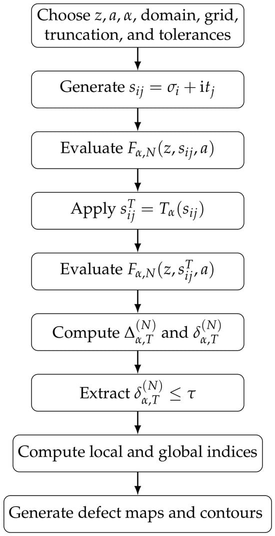
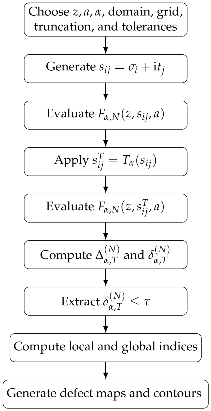
All computations (Figure 1) were performed in Python 3.12 using the NumPy and Matplotlib libraries in the IEEE double-precision complex arithmetic.

Figure 1. Workflow of the numerical computation.

The computational domain was discretized using a $400\times 400$ uniform grid in the complex plane.

The computations reported below used

$$N=450,N_{\sigma }=N_t=400,{\epsilon }_{\mathrm{reg}}={10}^{-14},\tau ={10}^{-8}.$$

Numerical stability was assessed by comparing the results with those obtained after increasing the truncation level N and refining the spatial grid.

Convergence and Validation

The truncation error was monitored through

$$E_N=\underset{s_{ij}\in \Omega }{\max }\left|F_{\alpha ,2N}(z,s_{ij},a)-F_{\alpha ,N}(z,s_{ij},a)\right|,$$

whereas the grid-refinement error was estimated by

$$E_{\mathrm{grid}}=\left|I_{\mathrm{glob}}^{(2N_{\sigma },2N_t)}-I_{\mathrm{glob}}^{(N_{\sigma },N_t)}\right|.$$

The computations were repeated after doubling the truncation level and refining the spatial grid. No significant changes were observed in the reported defect maps or in the global comparison index within the displayed numerical precision. These tests were used as a practical assessment of numerical stability for the illustrative computations presented below. As an internal validation, the numerical defect was required to vanish, up to truncation and roundoff errors, on the analytically known fixed-point line $\Re \left(s\right)=\alpha +{\displaystyle \frac{1}{2}}.$ The numerical parameters were increased until no significant changes were observed in either the defect maps or the comparison indices. Consequently, the reported computations may be regarded as numerically resolved for the purposes of the present work.

6.2. Comparison–Defect Maps and Calibration

The first numerical experiment illustrates the spatial behavior of the comparison defect associated with $T_{\alpha }$. At the fixed-point line

$$\Re \left(s\right)=\alpha +{\displaystyle \frac{1}{2}},$$

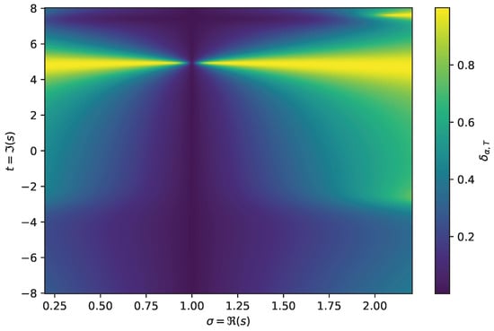
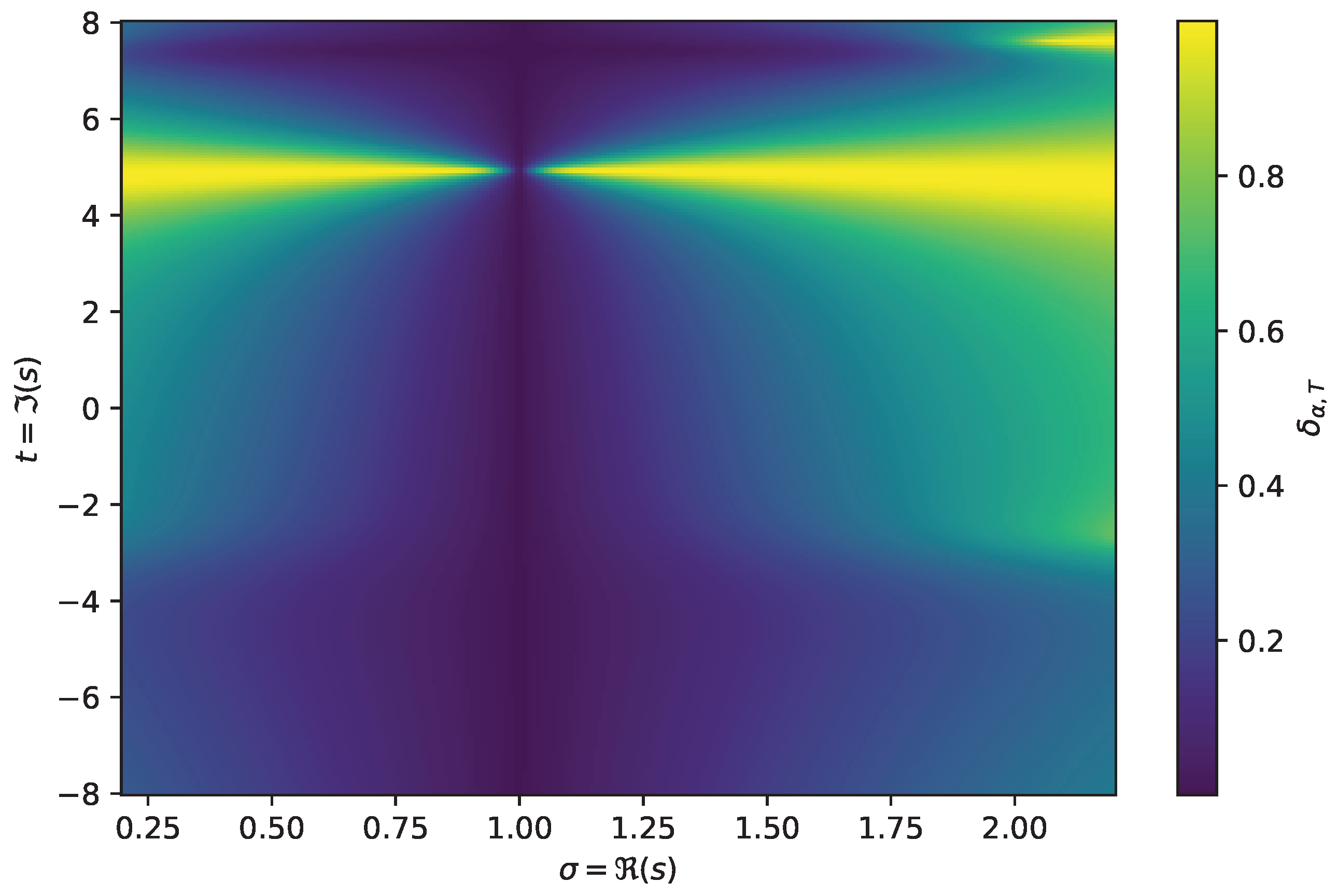
the defect vanishes identically for purely geometric reasons. Accordingly, the role of this line is to provide an exact calibration of the numerical implementation. The informative quantity is the off-axis variation of the normalized defect, which describes the function-dependent loss of comparison covariance. A representative defect map is shown in Figure 2.

Figure 2. Normalized numerical comparison defect ${\delta }_{\alpha ,T}^{\left(N\right)}(\sigma +it)$ for $\alpha =0.5$, $z=0.65e^{0.7i}$, and $a=1.2$. The vertical zero line $\sigma =1$ is the geometrically forced fixed-point set of $T_{\alpha }$ and is used as a calibration of the implementation; the off-axis profile is function-dependent.

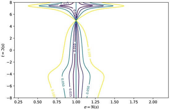
Figure 2 and Figure 3 show, respectively, the normalized comparison-defect map and representative contour levels. Since the zero on $\mathrm{Fix}\left(T_{\alpha }\right)$ is geometrically enforced, the function-dependent information is carried by the off-axis profile and by any additional zeros not belonging to the fixed-point set.

Figure 3. Contours of the normalized numerical comparison defect ${\delta }_{\alpha ,T}^{\left(N\right)}$ for the same parameters. The central line is the fixed-point baseline. The surrounding contours quantify approximate covariance away from that baseline and are not interpreted as a shifted critical strip.

6.3. Defect-Based Indices

The proposed indices provide a compact quantitative description of the comparison defect. The local index approaches unity in low-defect regions and decreases as the normalized discrepancy increases. The global index, being domain dependent, requires particular care when values corresponding to different fractional orders are compared. Indeed, the reflection transformation

$$T_{\alpha }\left(s\right)=1+2\alpha -\overline{s}$$

has the order-dependent fixed-point axis

$$\Re \left(s\right)=\alpha +{\displaystyle \frac{1}{2}}.$$

Consequently, if the global index is evaluated over a fixed domain in the s-plane while $\alpha$ varies, part of the observed variation may result from the displacement of the comparison axis relative to the computational domain rather than from the fractional deformation of the Lerch function itself. For this reason, in the present work we restrict the numerical discussion to the pointwise defect maps and low-defect contours, for which the geometrical meaning is unambiguous. A quantitative comparison of global defect-based indices across different fractional orders should instead be performed on co-moving domains centered on the corresponding reflection axis, for example,

$${\Omega }_{\alpha }(h,T)=\left\{s=\sigma +it:\left|\sigma -\alpha -{\displaystyle \frac{1}{2}}\right|\le h,\left|t\right|\le T\right\}.$$

Such a construction separates, as far as possible, the intrinsic dependence on the fractional order from the purely geometrical displacement of the comparison axis. A systematic investigation of this order-dependent global index is left for future studies.

The numerical experiments confirm the practical computability of the proposed defect-based framework. They reproduce the analytically prescribed comparison axis, illustrate the variation of the normalized defect away from it, and show how local regions of approximate comparison covariance can be represented through contour sets. These computations should be interpreted as numerical illustrations of the defect geometry rather than as evidence for an intrinsic order-dependent shift of a classical critical strip. More extensive comparisons between fractional orders and between different fractional operators require order-adapted computational domains and will be considered in future work.

7. A Concrete Spectral-Zeta Realization

To provide a concrete spectral realization of the preceding formulas, consider, for $a>2$, the diagonal operator

$$A_a:\mathcal{D}\left(A_a\right)\subset {\mathsf{\ell }}^2\left({\mathbb{N}}_0\right)⟶{\mathsf{\ell }}^2\left({\mathbb{N}}_0\right),$$

defined by

$$A_a{e}_n=(n+a)e_n,n=0,1,2,\dots ,$$

with domain

$$\mathcal{D}\left(A_a\right)=\left\{x={\left(x_n\right)}_{n\ge 0}\in {\mathsf{\ell }}^2\left({\mathbb{N}}_0\right):{\displaystyle \sum _{n=0}^{\infty }}{(n+a)}^2{\left|x_n\right|}^2<\infty \right\}.$$

The operator $A_a$ is positive and self-adjoint, with discrete spectrum [28,29]

$$\sigma \left(A_a\right)=\{n+a:n\in {\mathbb{N}}_0\}.$$

Its spectral zeta function is

$${\zeta }_{A_a}\left(s\right)=\mathrm{Tr}\left(A_a^{-s}\right)={\displaystyle \sum _{n=0}^{\infty }}{(n+a)}^{-s}=\zeta (s,a),\Re s>1.$$

Thus, the Hurwitz zeta function appearing in Section 5.3 is the spectral zeta function of an explicit operator rather than only a formal specialization of the Lerch transcendent. Proposition 1 yields

$$W_{+}^{\alpha }{\zeta }_{A_a}\left(s\right)={\displaystyle \sum _{n=0}^{\infty }}{\left[\log (n+a)\right]}^{\alpha }{(n+a)}^{-s}.$$

The parameter shift $a\mapsto a+1$ has a direct spectral interpretation. The spectrum of $A_{a+1}$ is obtained from that of $A_a$ by deleting the lowest eigenvalue a and relabelling the remaining eigenvalues. Therefore,

$${\zeta }_{A_a}\left(s\right)-{\zeta }_{A_{a+1}}\left(s\right)=a^{-s}.$$

Applying the right Weyl–Marchaud derivative and using the termwise formula proved above yields the exact relation

$$W_{+}^{\alpha }{\zeta }_{A_a}\left(s\right)-W_{+}^{\alpha }{\zeta }_{A_{a+1}}\left(s\right)={\left(\log a\right)}^{\alpha }{a}^{-s}.$$

(44)

Equation (44) provides a specific spectral conclusion: deleting the ground-state eigenvalue changes the fractionally differentiated spectral zeta function by precisely the Weyl weight associated with that eigenvalue.

There is also a direct spectral interpretation of the duplication identity. The spectrum $\{n+a:n\ge 0\}$ decomposes into its even and odd subsequences,

$$\{2n+a:n\ge 0\}\mathrm{and}\{2n+a+1:n\ge 0\}.$$

Factoring the scale 2 from the even and odd subsequences yields

$${\displaystyle \sum _{n=0}^{\infty }}{(2n+a)}^{-s}=2^{-s}\zeta \left(s,{\displaystyle \frac{a}{2}}\right),$$

and

$${\displaystyle \sum _{n=0}^{\infty }}{(2n+a+1)}^{-s}=2^{-s}\zeta \left(s,{\displaystyle \frac{a+1}{2}}\right).$$

Their sum is precisely the duplication identity in Equation (36). The nonzero defect obtained in Theorem 9 therefore quantifies the failure of the right Weyl–Marchaud derivative to preserve this even–odd spectral splitting covariance.

8. Conclusions

In this paper, a defect-based framework has been developed for studying the interaction between a fixed fractional derivative and comparison or covariance structures of Lerch-type functions. The construction deliberately separates arbitrary parameter comparisons from authentic functional identities. The former provide useful calibration diagnostics, whereas the latter are the appropriate setting in which a nonzero commutator can be interpreted as fractional symmetry breaking.

A principal analytical addition of the revised formulation is the explicit treatment of the full weighted-composition commutator. The multiplier term and the pullback term are distinct, and affine pullbacks in the spectral variable can be computed explicitly. In particular, a reflection reverses the orientation of the one-sided Weyl operator, which prevents an automatic commutation argument for reflection-type functional equations.

The general formalism is complemented by a non-elementary example based on the classical Hurwitz-zeta duplication formula. This identity defines an authentic finite weighted covariance. For $0<\alpha <1$, $a>2$, and $\Re s>1$, its fractional defect admits both a convergent Marchaud-integral representation and an explicit Dirichlet-series representation. On the real half-plane $s>1$, the defect is strictly positive. Hence the chosen right Weyl–Marchaud derivative does not preserve the classical duplication covariance there, and the region contains no zeros of the corresponding genuine duplication defect. This is a function-dependent consequence and is logically different from the fixed-point zeros generated by the prescribed comparison map.

The convergence argument has also been sharpened. In the absolutely convergent regimes used for the analytical applications, an explicit integrable majorant justifies interchange of the Lerch sum with the unbounded Weyl integral. In the conditionally convergent unit-circle regime, local uniform convergence of the logarithmically weighted series is retained, but the stronger interchange claim is no longer made without an additional tail hypothesis.

The elementary specialization $\Phi (0,s,a)=a^{-s}$ and the numerical defect maps remain useful as calibration benchmarks. In particular, the line $\Re s=\alpha +1/2$ remains the fixed-point set of the prescribed comparison map and is not interpreted as a displacement of the Riemann critical strip or of an abscissa of convergence. Finally, the affine-spectrum operator of Section 7 provides a concrete spectral-zeta realization of the Hurwitz formulas and gives an exact fractional relation for ground-state deletion. Further work may investigate other authentic Lerch covariances and other fractional operators, but such extensions require their operator domains and commutators to be verified separately.

References

- Apostol, T.M. Introduction to Analytic Number Theory; Springer: New York, NY, USA, 1976. [Google Scholar]
- Laurinčikas, A.; Garunkštis, R. The Lerch Zeta-Function; Kluwer Academic Publishers: Dordrecht, The Netherlands, 2002. [Google Scholar]
- NIST Digital Library of Mathematical Functions. Chapter 25: Zeta and Related Functions. Available online: https://dlmf.nist.gov/25 (accessed on 19 January 2026).
- Srivastava, H.M. A survey of some recent developments on higher transcendental functions of analytic number theory and applied mathematics. Symmetry 2021, 13, 2294. [Google Scholar] [CrossRef] [Scilit]
- Lerch, M. Note sur la fonction . Acta Math. 1887, 11, 19–24. [Google Scholar] [CrossRef]
- NIST Digital Library of Mathematical Functions. Section 25.14: Lerch’s Transcendent. Available online: https://dlmf.nist.gov/25.14 (accessed on 19 January 2026).
- Erdélyi, A.; Magnus, W.; Oberhettinger, F.; Tricomi, F.G. Higher Transcendental Functions; McGraw–Hill: New York, NY, USA, 1953; Volume 1. [Google Scholar]
- López, J.L.; Pérez Sinusía, E. New analytic representations of the Lerch transcendent. Numer. Algorithms 2026, 102, 1613–1634. [Google Scholar] [CrossRef] [Scilit]
- Ortigueira, M.D. A coherent approach to non-integer order derivatives. Signal Process. 2006, 86, 2505–2515. [Google Scholar] [CrossRef] [Scilit]
- Podlubny, I. Fractional Differential Equations; Academic Press: San Diego, CA, USA, 1999. [Google Scholar]
- Tenreiro Machado, J.A.; Kiryakova, V.; Mainardi, F. Recent history of fractional calculus. Commun. Nonlinear Sci. Numer. Simul. 2011, 16, 1140–1153. [Google Scholar] [CrossRef] [Scilit]
- Samko, S.G.; Kilbas, A.A.; Marichev, O.I. Fractional Integrals and Derivatives: Theory and Applications; Gordon and Breach: Yverdon, Switzerland, 1993. [Google Scholar]
- Li, C.; Dao, X.; Guo, P. Fractional derivatives in complex planes. Nonlinear Anal. Theory Methods Appl. 2009, 71, 1857–1869. [Google Scholar] [CrossRef] [Scilit]
- Závada, P. Operator of fractional derivative in the complex plane. Commun. Math. Phys. 1998, 192, 261–285. [Google Scholar] [CrossRef] [Scilit]
- Cattani, C. Family of Curves based on Riemann zeta function. In Computational Science and Its Applications—ICCSA 2011. Lecture Notes in Computer Science; Murgante, B., Gervasi, O., Iglesias, A., Taniar, D., Apduhan, B.O., Eds.; Springer: Berlin/Heidelberg, Germany, 2011; Volume 6785, pp. 644–657. [Google Scholar]
- Cattani, C.; Guariglia, E. Fractional derivative of the Hurwitz ζ function and chaotic decay to zero. J. King Saud Univ.-Sci. 2015, 28, 75–81. [Google Scholar] [CrossRef] [Scilit]
- Cattani, C.; Guariglia, E.; Wang, S. On the critical strip of the Riemann zeta fractional derivative. Fundam. Inform. 2017, 151, 459–472. [Google Scholar] [CrossRef] [Scilit]
- Fernandez, A.; Djida, J.-D. Fractional differential relations for the Lerch zeta function. Arch. Math. 2021, 117, 515–527. [Google Scholar] [CrossRef] [Scilit]
- Cai, X.S.; López, J.L. A note on the asymptotic expansion of the lerch’s transcendent. Integral Transform. Spec. Funct. 2019, 30, 844–855. [Google Scholar] [CrossRef] [Scilit]
- Edwards, H.M. Riemann’s Zeta Function; Dover Publications Inc.: Garden City, NY, USA, 2003. [Google Scholar]
- Titchmarsh, E.C. The Theory of the Riemann Zeta-Function, 2nd ed.; Oxford University Press: Oxford, UK, 1986. [Google Scholar]
- NIST Digital Library of Mathematical Functions. Section 25.11: Hurwitz zeta Function. Available online: https://dlmf.nist.gov/25.11 (accessed on 19 January 2026).
- Lewin, L. Polylogarithms and Associated Functions; North-Holland: New York, NY, USA, 1981. [Google Scholar]
- NIST Digital Library of Mathematical Functions. Section 25.12: Polylogarithms. Available online: https://dlmf.nist.gov/25.12 (accessed on 19 January 2026).
- Singh, R.K.; Kumar, R.D.C. Weighted composition operators on functional Hilbert spaces. Bull. Aust. Math. Soc. 1985, 31, 117–126. [Google Scholar] [CrossRef] [Scilit][Green Version]
- Olver, P.J. Applications of Lie Groups to Differential Equations, 2nd ed.; Springer: Berlin/Heidelberg, Germany, 1993. [Google Scholar]
- Lee, J.M. Introduction to Smooth Manifolds, 2nd ed.; Springer: Berlin/Heidelberg, Germany, 2013. [Google Scholar]
- Kato, T. Perturbation Theory for Linear Operators; Springer: Berlin/Heidelberg, Germany, 1995; Volume 2. [Google Scholar]
- Reed, M.; Simon, B. Methods of Modern Mathematical Physics I: Functional Analysis; Academic Press: Cambridge, MA, USA, 1980. [Google Scholar]
Disclaimer/Publisher’s Note: The statements, opinions and data contained in all publications are solely those of the individual author(s) and contributor(s) and not of MDPI and/or the editor(s). MDPI and/or the editor(s) disclaim responsibility for any injury to people or property resulting from any ideas, methods, instructions or products referred to in the content. |
© 2026 by the author. Licensee MDPI, Basel, Switzerland. This article is an open access article distributed under the terms and conditions of the Creative Commons Attribution (CC BY) license.