CoSafe-Nav: An Intelligent Connectivity-Aware Navigation System for UAVs in Perception-Degraded Environments

Abstract

Reliable UAV navigation is challenging when direct geometric perception is limited and only sparse environmental observations are available. This paper presents CoSafe-Nav, an integrated navigation framework that uses ultra-wideband (UWB) line-of-sight (LOS) observations to construct a candidate corridor and guide trajectory generation. The framework addresses fixed-altitude planar navigation with known, pre-deployed anchors and an available UAV pose estimate. LOS-supported segments are accumulated online, and a grid-based Euclidean distance transform (EDT) provides a common clearance representation for path ranking and trajectory refinement. The path planner combines travel distance with a local inverse-distance penalty. The trajectory stage corrects interior control points using the EDT gradient, regenerates the spatial curve, and assigns execution timing. Evaluation comprises two simulation scenarios, component comparisons, an anchor-availability study, and indoor UAV trials. CoSafe-Nav completed all ten navigation tasks in each simulation scenario and four of five indoor trials. In the path-planning comparison, mean EDT corridor clearance increased from 0.76 to 0.98 m and from 0.63 to 0.91 m, accompanied by longer routes. These means describe successful tasks within each configuration. The trajectory comparison also showed a lower acceleration integral for the safety-guided method. The results support the feasibility of the integrated processing chain under the stated pre-instrumented deployment conditions.

1. Introduction

Unmanned aerial vehicles (UAVs) are used in disaster response, environmental inspection, underground exploration, and infrastructure monitoring [1,2,3]. These applications motivate research on limited-perception navigation; the present system specifically addresses pre-instrumented environments with known UWB anchors, an available pose estimate, and fixed-altitude planar motion. In many of these applications, global navigation satellite system (GNSS) signals are unavailable or unreliable because of indoor operation, underground structures, urban canyons, or severe occlusion. Direct geometric perception is also difficult to maintain. Low illumination, weak texture, smoke, and dynamic occlusion challenge vision-based sensing, while LiDAR deployment involves sensing-range, hardware, and onboard-computation constraints. Under these conditions, a UAV must make navigation decisions from incomplete and indirect observations rather than from a complete geometric map [1,2].

Path planning and trajectory generation methods are commonly developed under the assumption that a reliable occupancy map, point-cloud map, or continuous distance field is available. Graph-search methods such as A* provide deterministic solutions but are sensitive to the completeness and resolution of the map. Sampling-based and continuous optimization methods can generate feasible trajectories in complex spaces, but their collision checking and safety optimization also depend on sufficiently informative geometric observations. Path search and trajectory generation therefore depend on both the represented free space and the clearance criterion applied to it. A navigation system for perception-degraded environments should therefore address environmental representation, safe path search, and executable trajectory generation as a coupled problem.

Ultra-wideband (UWB) technology has been widely used for indoor localization and GNSS-denied navigation because of its accurate ranging and relatively robust communication characteristics [4]. Existing UWB-based navigation studies mainly use range or pose information for localization and relative navigation [5,6,7]. However, the connectivity state between a UAV and a UWB anchor can also provide indirect information about the surrounding spatial structure. A line-of-sight (LOS) classification is used as conditional support for an unobstructed link direction, whereas a non-line-of-sight (NLOS) state supplies no positive free-space support. A radio label alone does not establish that a finite UAV body can pass along the link. Although such connectivity observations do not reconstruct complete geometry, they can be transformed into a task-oriented representation of traversable space.

This paper proposes CoSafe-Nav, an intelligent UWB connectivity-aware navigation system for UAVs in perception-degraded environments. The system uses sequences of LOS/NLOS observations to construct directional corridor support and combines this representation with an explicit corridor-clearance model for route selection. CoSafe-Nav accumulates LOS-supported free-space segments into a traversable corridor, applies a Euclidean distance transform (EDT) to represent distance to unsupported corridor cells, and uses the resulting field in both path planning and trajectory refinement. The study evaluates this information flow in pre-instrumented planar environments using corridor-clearance, computation-time, and task-completion metrics.

The contributions are:

• A connectivity-derived corridor representation that accumulates LOS-supported segments while distinguishing positive free-space support from NLOS or unavailable observations.
• A planning and refinement pipeline that uses the same EDT representation for local path ranking and sampled trajectory correction, followed by time allocation and flight-control delivery.
• A feasibility evaluation comprising two simulation task sets, path and trajectory comparisons, an anchor-availability study, and five indoor trials. The evaluation characterizes execution and corridor-clearance behavior within the stated sensing assumptions.

The remainder of this paper is organized as follows. Section 2 reviews UWB-based navigation, safe planning, and trajectory generation, and their roles in the navigation pipeline. Section 3 and Section 4 define the system model and present the connectivity-to-execution pipeline. Section 5 describes the evaluation protocols, and Section 6 reports and discusses the simulation and indoor-platform results together with the application scope and future work. Section 7 concludes the paper.

2. Related Work

Existing studies largely address separate stages of the navigation pipeline: UWB-based localization, geometric mapping, path planning, or trajectory generation. We therefore distinguish state estimation from traversability representation and focus on how planning and trajectory generation use environmental constraints.

2.1. UWB-Based Navigation and Connectivity-Aware Perception

UWB systems provide accurate time-of-flight or time-difference measurements and have been used for indoor localization, relative positioning, and sensor fusion. Surveys report that UWB offers a favorable combination of ranging accuracy and robustness in challenging indoor environments, while also emphasizing practical issues such as interoperability, channel access, antenna configuration, and ranging-protocol design [4,8]. Representative visual–inertial and LiDAR odometry systems include ORB-SLAM [9], ORB-SLAM3 [10], VINS-Mono [11], LOAM [12], FAST-LIO [13], FAST-LIO2 [14], and FAST-LIVO [15]. These systems combine visual, inertial, or LiDAR observations for state estimation. CoSafe-Nav instead takes the pose estimate as an input to connectivity-based corridor construction.

Recent studies have combined UWB with inertial or visual information to improve localization robustness. Kao et al. developed a visual–inertial–UWB fusion network for indoor UAV localization [5]. Zeng et al. used double UWB tags and an IMU for localization relative to a landing platform [6], while Zheng et al. investigated UWB–VIO fusion for relative localization in robot teams [7]. These studies demonstrate the value of UWB when visual tracking is intermittent or when a common spatial reference is needed. Their primary outputs, however, remain pose, position, or relative displacement estimates. They do not by themselves specify which regions are traversable or how a UAV should maintain clearance from partially observed obstacles. UWB therefore solves an important state-estimation problem, but leaves the state-to-navigation interface open.

NLOS identification has likewise been studied mainly as a localization problem because multipath and obstruction can introduce significant ranging errors. Feature-based statistical modeling has been used for NLOS detection [16], support-vector methods have been applied to LOS/NLOS localization [17], and transformer-based classifiers have been developed for NLOS identification and ranging mitigation [18]. From this perspective, NLOS is an undesirable measurement condition to be detected or corrected. In CoSafe-Nav, an NLOS observation supplies no positive support for adding corridor cells. The limitation is that a connectivity label is not equivalent to a geometric obstacle boundary: it can be affected by obstruction, multipath, antenna orientation, or transient radio conditions. A useful navigation method must therefore exploit the structural information without treating a single LOS/NLOS decision as complete scene understanding.

UWB–IMU fusion has also been used for indoor quadrotor localization, providing a relevant state-estimation baseline for connectivity-aware navigation [19]. The unresolved issue is how to convert incomplete directional relations into a task-oriented representation that can support planning without treating each connectivity decision as a deterministic obstacle label.

2.2. Safe Path Planning and Trajectory Generation

Classical and sampling-based planners provide well-established ways to search a represented configuration space. A* offers an interpretable minimum-cost graph search [20], whereas D* Lite supports efficient updates when edge costs change [21]. RRT explores complex or higher-dimensional spaces through randomized tree expansion [22]; RRT* introduces asymptotic optimality [23]; and Informed RRT* focuses sampling after an initial solution is found [24]. Their common prerequisite is a sufficiently informative representation of free and occupied space. Graph and sampling-based searches operate on the free-space constraints supplied by their environment representation. In CoSafe-Nav, the search domain is the connectivity-derived corridor, and EDT clearance enters the node-ranking score.

Distance transforms and signed distance fields address the safety weakness of binary planning by assigning clearance information to free space. Occupancy grids provide a probabilistic spatial representation [25]. Voxblox incrementally constructs Euclidean signed distance fields for onboard MAV planning [26], whereas FIESTA provides an incremental Euclidean distance-field framework for online aerial-robot motion planning [27]. An EDT can serve as a soft cost, a hard constraint, or a gradient source. The remaining limitation is upstream: a distance field is only as reliable as the occupancy or traversability representation from which it is computed. Dense geometric sensing can provide that input, but sparse radio connectivity does not automatically do so. Therefore, a safety-aware planner for the present problem must address both the construction of the representation and the use of the clearance field.

The same issue appears when a discrete route is converted into a flight trajectory. Minimum-snap generation improves smoothness through derivative-cost minimization [28]. Polynomial trajectory planning incorporates waypoint and dynamic constraints [29], while uniform B-spline replanning supports efficient online trajectory updates [30]. Yet these methods generally assume that the input waypoints and free-space constraints are already reliable. Piecewise cubic interpolation provides continuity, while an EDT term supplies a separate corridor-clearance criterion. CoSafe-Nav applies this criterion during trajectory correction and checks the re-smoothed curve at sampled positions.

EGO-Planner performs ESDF-free local trajectory optimization [31], while FASTER supports fast and safe replanning in unknown environments [32]. Safe-flight-corridor planning constructs dynamically feasible quadrotor trajectories within collision-free regions [33], and CMPCC combines corridor constraints with model predictive contouring control [34]. These methods improve online execution through local optimization or explicit spatial and dynamic constraints. They are effective when depth, LiDAR, or another geometric source provides a sufficiently detailed local environment. In the present setting, the unresolved issue lies upstream: a local optimizer cannot enforce clearance that has not first been inferred from sparse connectivity. CoSafe-Nav uses the same corridor EDT in both path search and trajectory refinement.

2.3. System-Level Navigation in Perception-Degraded Environments

Navigation with limited perception requires coordination between state estimation, environment representation, planning, and execution. Geometric navigation systems address this coordination using incremental distance fields, local trajectory optimization, or explicit flight corridors [26,27,31,33]. CoSafe-Nav considers a different representation input: sparse radio link states. Its design question is how to carry this indirect evidence through route selection and trajectory generation without equating radio visibility with a complete geometric map.

The proposed system maintains separate interfaces for pose estimation and link classification, corridor and EDT updates, discrete path search, and trajectory delivery. Reusing the corridor EDT keeps the clearance quantity consistent between search and refinement. The resulting implementation is evaluated as an integrated navigation pipeline; the experiments do not isolate every interaction between its modules.

2.4. Research Gap and Position of This Work

These methods provide established tools for localization, geometric planning, and trajectory generation, but they do not specify how sparse LOS relations can define a planning corridor. This study focuses on that interface under known-anchor, fixed-altitude planar-motion assumptions. The individual search, distance-transform, and interpolation operations are standard; the contribution is their integration with link-state evidence.

CoSafe-Nav converts LOS observations into candidate free-space segments, updates their union, computes a corridor EDT, and uses it in path ranking and trajectory refinement. The system comparison examines complete task execution, while the path and trajectory comparisons describe behavior at the corresponding module interfaces. Anchor removal characterizes dependence on observation availability. The indoor trials assess whether the same processing chain can operate during flight. Representation accuracy and body-aware physical clearance are included in the future work described in Section 6.6.

3. System Model and Overview

3.1. Problem Formulation

Consider a planar workspace containing a set of pre-deployed UWB anchors, denoted as $\mathcal{A}=\{a_1,\dots ,a_N\}$, where the anchor coordinates $a_i\in {\mathbb{R}}^2$ are known in the navigation frame. The UAV position estimate at time t is $x_t={[x_t^{\left(1\right)},x_t^{\left(2\right)}]}^{\mathsf{T}}\in {\mathbb{R}}^2$, and the target is $x_g={[x_g^{\left(1\right)},x_g^{\left(2\right)}]}^{\mathsf{T}}\in {\mathbb{R}}^2$. The formulation represents horizontal motion at a prescribed flight altitude; altitude stabilization is handled by the flight-control layer rather than by the planar planner. Let ${\mathcal{A}}_t\subseteq \mathcal{A}$ denote the anchors for which a link-state observation is available at time t. For each $a_i\in {\mathcal{A}}_t$, the observed state is

$$l_i\left(x_t\right)\in \{0,1\},a_i\in {\mathcal{A}}_t,$$

(1)

where $l_i\left(x_t\right)=1$ denotes an LOS connection, and $l_i\left(x_t\right)=0$ denotes an observed NLOS connection. An anchor outside ${\mathcal{A}}_t$ is unavailable rather than NLOS and is not used in the current map update. The available observation set is ${\mathcal{L}}_t=\{(a_i,l_i\left(x_t\right)):a_i\in {\mathcal{A}}_t\}$. The method takes a usable pose estimate as an input and processes whichever anchor observations are available; it does not require all anchors to be observed simultaneously. A nonempty observation set alone does not ensure that the inferred corridor connects the start and goal. The objective is to infer a task-oriented candidate traversable representation from ${\left\{{\mathcal{L}}_{\tau }\right\}}_{\tau =0}^t$ and generate a trajectory T from $x_0$ to $x_g$ with specified nominal velocity and acceleration limits as design requirements. The time-allocation rule and the role of these design requirements are described in Section 4.4.

3.2. CoSafe-Nav Architecture

The system follows the processing chain

$${\mathcal{L}}_t\to M_{\mathrm{corr}}^t\to D_t\left(p\right)\to P_t\to T_t,$$

(2)

where $M_{\mathrm{corr}}^t$ is the incrementally updated binary corridor map, $D_t\left(p\right)$ is its EDT field, $P_t$ is the current discrete path, and $T_t$ is the continuous trajectory. UWB measurements are separated into two information streams in the prototype: the localization module supplies the pose estimate, whereas the link-state module supplies LOS/NLOS decisions. The environment-modeling module converts LOS-supported rays into candidate traversable cells, subject to the rasterization assumptions discussed below. The planning module searches those cells using distance and corridor-clearance costs, and the trajectory module refines and time-parameterizes the path before sending it to the flight-control interface.

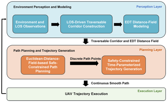
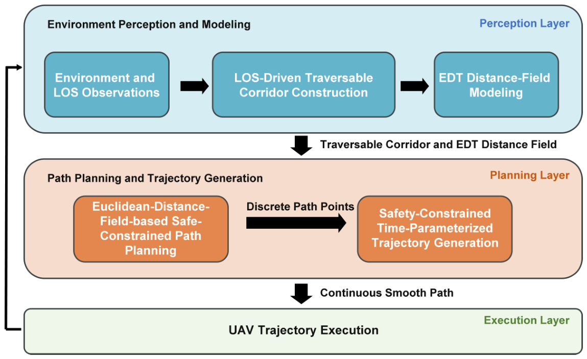
Figure 1 shows the system-level architecture. It emphasizes the separation between the perception layer, the planning layer, and the execution layer, while also showing how the traversable corridor and EDT field are passed to path planning and trajectory generation.

Figure 1. System architecture of the UWB connectivity-aware navigation and trajectory-generation framework.

4. Methods

4.1. LOS-Driven Traversable-Corridor Construction

Each rasterized LOS cell is expanded to its $3\times 3$ neighboring-cell footprint before the EDT is recomputed.

The continuous workspace is discretized into a finite set $\mathcal{G}$ of grid-cell centers in metric coordinates. Here $p\in \mathcal{G}$ denotes a grid-cell center, and $M_{\mathrm{corr}}^t\left(p\right)\in \{0,1\}$ is the corresponding binary corridor-map value. A value of one denotes a cell provisionally supported by at least one LOS observation; a value of zero denotes a cell that is unobserved or unsupported. The representation therefore does not distinguish a physical obstacle from an unknown cell and must not be interpreted as a complete occupancy map.

For an available LOS observation to anchor, $a_i$, the candidate free-space segment is

$${\mathcal{S}}_i\left(x_t\right)=\left\{p\mid p=x_t+s(a_i-x_t),0\le s\le 1\right\}.$$

(3)

The cells intersected by this segment are obtained by grid-line rasterization and added to the corridor. The implementation maintains this connectivity-derived map separately from the simulator’s ground-truth obstacle grid; ground truth is used to generate LOS/NLOS observations and evaluate the result, but is not copied into the planner’s perceived map. Let ${\mathcal{C}}_t=\{p\in \mathcal{G}:M_{\mathrm{corr}}^t\left(p\right)=1\}$ denote the supported-cell set, let ${\mathcal{I}}_t=\{i:a_i\in {\mathcal{A}}_t,l_i\left(x_t\right)=1\}$, and let $\mathcal{R}\left({\mathcal{S}}_i\right)\subseteq \mathcal{G}$ denote the rasterized cells. The update is

$${\mathcal{C}}_t={\mathcal{C}}_{t-1}\cup \bigcup _{i\in {\mathcal{I}}_t}\mathcal{R}\left({\mathcal{S}}_i\left(x_t\right)\right),M_{\mathrm{corr}}^t\left(p\right)=\mathbf{1}[p\in {\mathcal{C}}_t].$$

(4)

The prototype can initialize $M_{\mathrm{corr}}^0$ from available LOS relations among deployed anchors; subsequent UAV–anchor observations expand it online. This is a monotonic corridor-update rule: once a cell has received LOS support, it remains in the corridor for the current mission.

This abstraction assumes that the link geometry is relevant to the flight plane and that the LOS label is sufficiently reliable. Neither a clear line nor a line-intersected grid cell certifies clearance for the airframe and propellers. Vertical obstacle structure, anchor–UAV height differences, antenna placement, and material-dependent propagation are not resolved by the planar map. Observed NLOS and unavailable links add no free-space segment and do not retract earlier support. The monotonic update therefore depends on the validity of its positive LOS evidence.

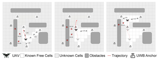
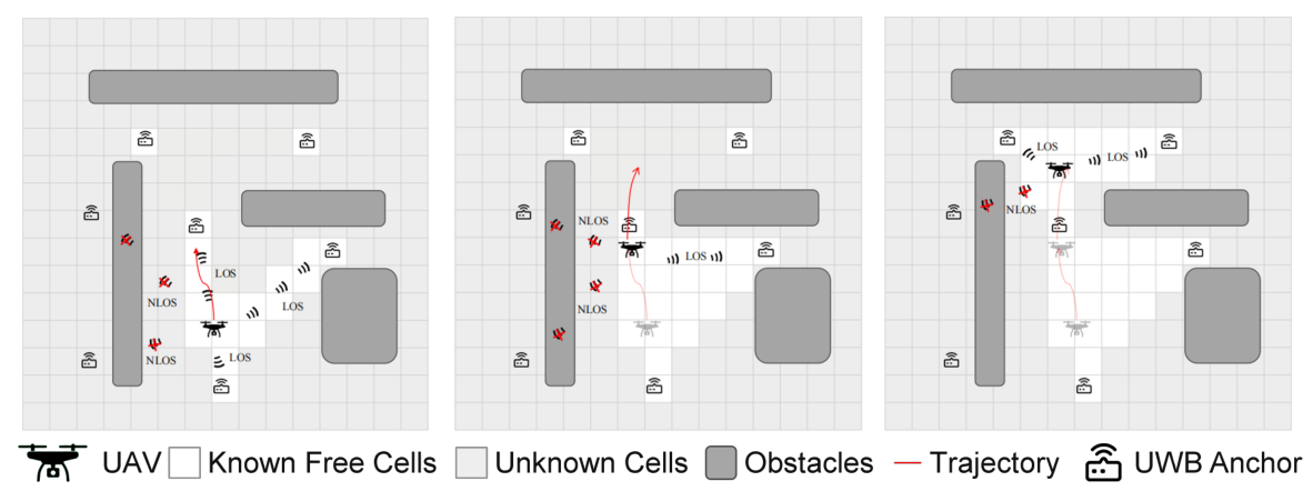
The progressive accumulation of LOS-supported cells and the resulting corridor updates are illustrated in Figure 2.

Figure 2. Progressive construction of the LOS-driven traversable corridor under sequential LOS/NLOS connectivity observations. The red arrows indicate the UAV trajectory or movement direction, while the red crosses denote blocked or unreliable UWB measurements caused by obstacles under non-line-of-sight (NLOS) conditions.

4.2. EDT-Based Clearance Field

Let ${\mathcal{B}}_t=\mathcal{G}\setminus {\mathcal{C}}_t$ contain all unsupported or out-of-corridor grid-cell centers in the planning grid. For a supported cell center, p, the grid EDT is

$$D_t\left(p\right)=\underset{b\in {\mathcal{B}}_t}{min}{\parallel p-b\parallel }_2.$$

(5)

The value $D_t\left(p\right)$ is the distance to the nearest unsupported grid-cell center, expressed in meters. It provides a discretized corridor-clearance measure, not a reconstruction of physical obstacle geometry or an unconditional lower bound on body clearance. References to corridor clearance below use this grid-based definition. For a continuous sample, q, the implementation converts $(q_x,q_y)$ to the containing grid-cell index and queries the corresponding cell value (nearest-cell lookup). The numerical gradient is estimated by centered finite differences with step $h=max(\Delta g,{10}^{-3}\mathrm{m})$, where $\Delta g$ is the grid resolution; out-of-grid or unknown queries return zero EDT for the safety check and statistics. Thus, the implementation does not use bilinear interpolation or a continuous physical distance field.

Within supported space, the distance field ranks central corridor cells above cells adjacent to unsupported regions. This supplies a graded preference beyond the binary membership test. The field is recomputed when LOS observations change the corridor. Its numerical resolution and the reliability of the underlying LOS evidence both affect the interpretation of the resulting margins.

The parameter $d_{\mathrm{safe}}$ specifies the sampled EDT margin used by the trajectory implementation. In the experimental configuration, $d_{\mathrm{safe}}=0.20$ m. Path search instead applies the soft inverse-distance penalty below rather than excluding every supported cell with $D_t<d_{\mathrm{safe}}$. The path-search domain therefore includes supported cells below the trajectory-correction margin. The reported $D_{min}$ and $D_{\mathrm{mean}}$ summarize this EDT quantity.

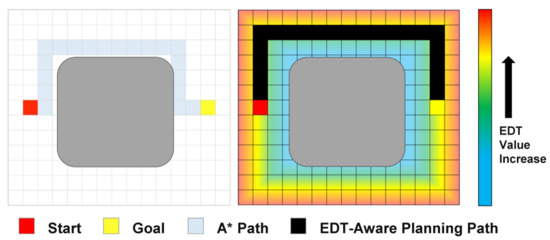
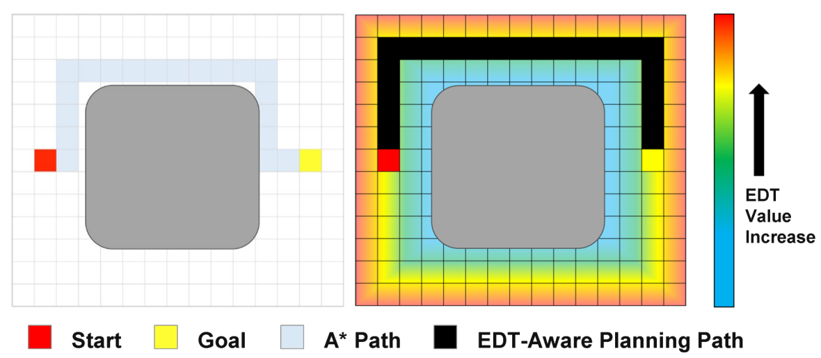
Figure 3 illustrates the difference between a conventional shortest path and the EDT-aware route. The A* path is shorter in the depicted geometry but follows the inferred corridor boundary. The EDT-aware route departs from the shortest route and uses the higher-clearance portion of the supported region. The figure is a conceptual visualization of the planning analysis; the quantitative comparison is presented in Section 6.2.

Figure 3. Illustration of conventional shortest-path planning and EDT-aware planning. The grid distance field supplies a graded preference for greater corridor clearance.

4.3. EDT-Aware Path Planning

The path-ranking rule combines accumulated travel distance with a local clearance penalty. Let $G_{\mathrm{dist}}$ denote accumulated distance and F denote the node-ranking score:

$$G_{\mathrm{dist}}\left(v\right)\leftarrow min\{G_{\mathrm{dist}}\left(v\right),G_{\mathrm{dist}}\left(u\right)+\ell (u,v)\},$$

(6)

where u is the current node, v is a supported successor, $\ell (u,v)={\parallel v-u\parallel }_2$, and $G_{\mathrm{dist}}\left(x_0\right)=0$; other distance labels are initialized to infinity. For a partial path $(p_0,\dots ,p_K)$ ending at $p_K=n$, its accumulated distance is

$$G_{\mathrm{dist}}\left(n\right)={\displaystyle \sum _{k=1}^K}{\parallel p_k-p_{k-1}\parallel }_2,$$

(7)

$$\varphi \left(n\right)={\displaystyle \frac{1}{D_t\left(n\right)+\epsilon }},$$

(8)

$$F\left(n\right)=G_{\mathrm{dist}}\left(n\right)+\lambda \varphi \left(n\right)+h\left(n\right),h\left(n\right)={\parallel n-x_g\parallel }_2.$$

(9)

With $\epsilon >0$ and $\lambda \ge 0$, the local penalty $\varphi \left(n\right)$ is not a sum along the partial path. Accordingly, F is a ranking score rather than a cumulative safety objective. If distances are expressed in meters, $\epsilon$ has units of meters and $\lambda$ has units of square meters. The search prioritizes nodes using this local score; the cumulative distance label remains separate. An eight-connected grid uses axial and diagonal distances scaled by the grid resolution; unsupported cells are excluded.

The distance-only comparator omits the local EDT penalty while retaining the same grid neighborhood. The safety term changes search priority rather than correcting a route only after search. The ranking parameters are $\lambda =0.04{\mathrm{m}}^2$ and $\epsilon =0.001$ m. The comparison evaluates this local ranking rule; its objective is distinct from an accumulated clearance cost.

4.4. Safety-Guided Trajectory Generation

The discrete route is converted into an initial spatial curve $T\left(s\right)$, parameterized by spatial arc length $s\in [0,S]$, where S is the curve length. The curve is constructed from the route points and subsequently represented by control points for refinement:

$$T\left(s_k\right)=p_k,k=0,\dots ,K.$$

(10)

The spatial smoothness criterion is written as

$$J_{\mathrm{smooth}}\left(T\right)={\int }_0^S{\parallel T^{″}\left(s\right)\parallel }_2^2\mathrm{d}s.$$

(11)

After time parameterization $x\left(t\right)=T\left(s\right(t\left)\right)$, the nominal motion requirements are

$$\parallel \dot{x}{\left(t\right)\parallel }_2\le v_{max},{\parallel \ddot{x}\left(t\right)\parallel }_2\le a_{max},$$

(12)

with endpoint conditions $x\left(0\right)=p_0$, $x\left(T_f\right)=p_K$, $\dot{x}\left(0\right)=0$, and $\dot{x}\left(T_f\right)=0$. The present implementation uses these values as nominal design settings for timing and control; it does not independently report continuous-trajectory peak velocity or acceleration. The experimental metrics therefore comprise completion counts, sampled corridor clearance, and derivative integrals, as defined in Section 5.1; the integral metrics must not be interpreted as verification of the peak limits.

For each refinement iteration, r, let $s_j$ denote the arc-length location of the jth checked sample, and let $J_r$ be the number of checked samples at that iteration. For every sample, $q_j^r=T^r\left(s_j\right)$, with $D_t\left(q_j^r\right)<d_{\mathrm{safe}}$, let $g_j^r$ be the normalized EDT gradient at that sample. The sample correction is accumulated on the interior control points associated with the containing route segment:

$$g_j^r={\displaystyle \frac{\nabla D_t\left(q_j^r\right)}{\parallel \nabla D_t\left(q_j^r\right){\parallel }_2}},\Delta c_k^r+=\frac{1}{2}{\delta }_{\mathrm{ref}}{g}_j^r,\Delta c_{k+1}^r+=\frac{1}{2}{\delta }_{\mathrm{ref}}{g}_j^r,$$

(13)

where the second update is applied only when the corresponding control point is interior. The updated control points are

$$c_i^{r+1}=c_i^r+\Delta c_i^r,i=1,\dots ,K-1.$$

(14)

Here, $c_i^r$ denotes the ith control point, k is the segment index associated with sample $q_j^r$, and ${\delta }_{\mathrm{ref}}$ is the fixed correction step. Samples with a zero numerical gradient are skipped. After the accumulated updates are applied, a centripetal Catmull–Rom curve is regenerated with the start and goal points retained. The numerical correction settings and stopping criteria are presented in Section 5.5.

The sampled clearance target is $D_t\left(q_j\right)\ge d_{\mathrm{safe}}$ for all checked samples $q_j$, where $j=1,\dots ,J_r$ at refinement iteration r. The implementation samples the curve at the controller period $\Delta t=0.02$ s (50 Hz); because the spatial speed is assigned locally, the corresponding arc-length spacing is approximately $v_k\Delta t$ on segment k, with $v_k$ defined below. Refinement stops when all samples satisfy $D_t\left(q_j\right)\ge d_{\mathrm{safe}}-{\tau }_D$ or when the maximum of $N_{\mathrm{iter}}=20$ iterations is reached. Reaching the iteration cap alone does not establish feasibility. The stopping criterion concerns sampled corridor clearance and does not impose a route-topology constraint.

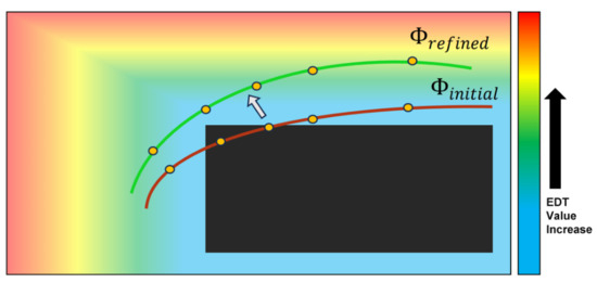
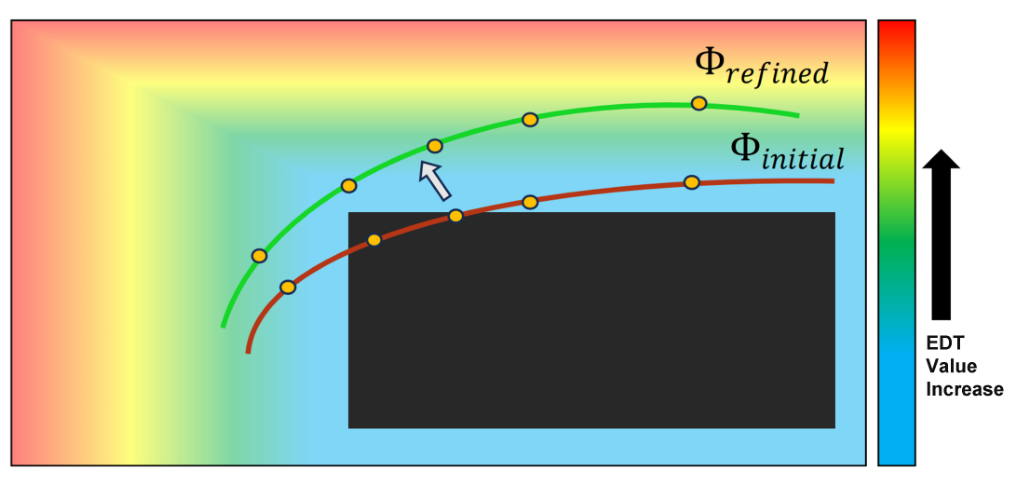
The control-point correction and curve-regeneration procedure are illustrated in Figure 4.

Figure 4. Illustration of EDT-guided trajectory refinement. The color field represents distance to unsupported corridor cells; the dark region denotes unsupported space in this schematic. The white arrow indicates the direction of path refinement from the initial trajectory ${\mathsf{\Phi }}_{\mathrm{initial}}$ to the refined trajectory ${\mathsf{\Phi }}_{\mathrm{refined}}$. Curve samples identify low-clearance regions, whose corrections are accumulated on interior control points before the curve is regenerated and checked again. The curves illustrate the correction mechanism rather than continuous body clearance.

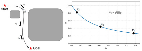
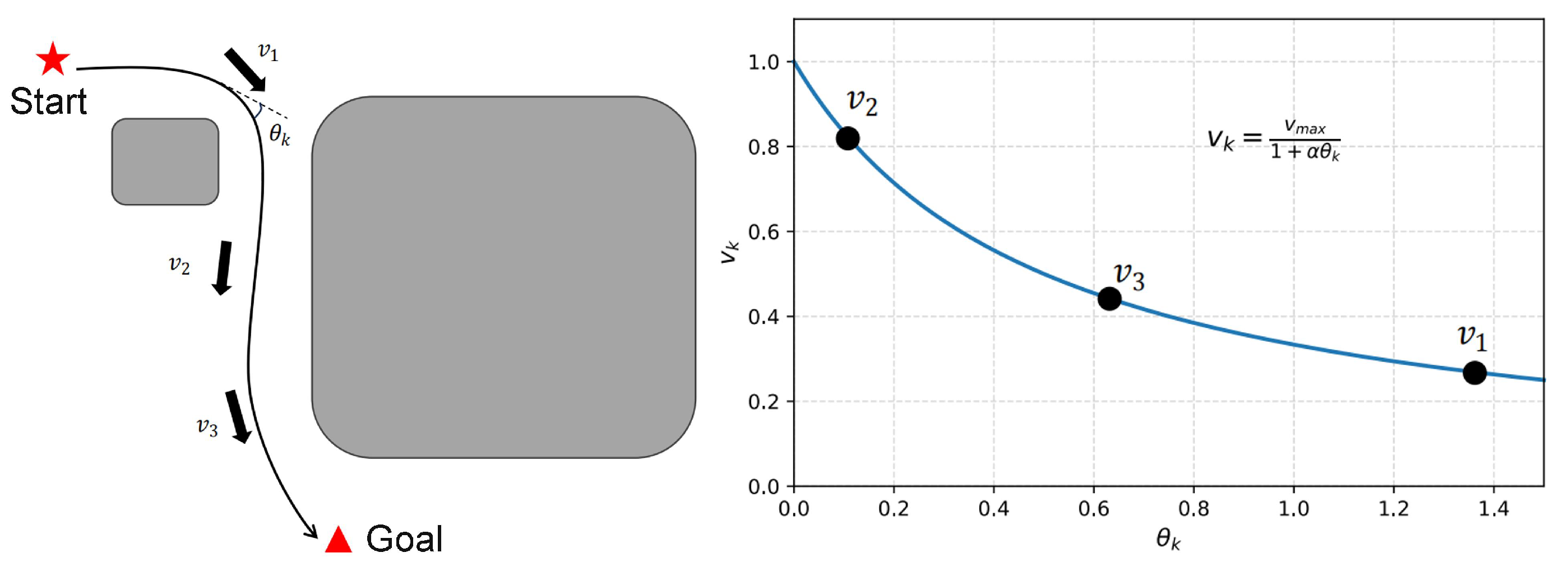
Figure 5 illustrates the implemented turning-angle-based time allocation. For an interior route point, $p_k$, the local turning angle is

$${\theta }_k=arccos\left({\displaystyle \frac{{(p_k-p_{k-1})}^{\mathsf{T}}(p_{k+1}-p_k)}{\parallel p_k-p_{k-1}{\parallel }_2{\parallel p_{k+1}-p_k\parallel }_2+{\epsilon }_{\theta }}}\right),$$

(15)

where ${\theta }_k$ measures the local change in direction, ${\epsilon }_{\theta }$ is a positive numerical regularizer with units of ${\mathrm{m}}^2$, and $k=1,\dots ,K-1$. The local execution speed on segment k is

$$v_k={\displaystyle \frac{v_{max}}{1+\alpha {\overline{\theta }}_k}},$$

(16)

where $v_{max}$ is the allowed reference speed, $\alpha$ is the nonnegative turning-angle sensitivity with units of ${\mathrm{rad}}^{-1}$, and ${\overline{\theta }}_k$ is the angle assigned to segment k: ${\overline{\theta }}_0={\theta }_1$, ${\overline{\theta }}_k={\theta }_k$ for $1\le k\le K-2$, and ${\overline{\theta }}_{K-1}={\theta }_{K-1}$. Thus, larger turning angles produce lower local speeds. The duration of segment k is $\Delta t_k={\parallel p_{k+1}-p_k\parallel }_2/v_k$, and the total execution time is $T_f={\sum }_{k=0}^{K-1}\Delta t_k$. Commands are issued every $\Delta t=0.02$ s (50 Hz). The yaw controller uses a $0.2$ s look-ahead and limits the yaw-rate command to $1.2$ rad/s. These settings define the nominal timing and heading updates; they do not by themselves verify the continuous velocity or acceleration limits.

Figure 5. Illustration of the turning-angle-dependent time allocation used for trajectory execution. ${\theta }_k$ is a local turning angle, $v_k$ is the corresponding local execution speed, $v_{max}$ is the reference speed limit, and $\alpha$ is the turning-angle sensitivity coefficient. Larger turning angles lead to lower local speeds and longer segment durations.

In particular, $\ddot{x}=T^{″}\left(s\right){\dot{s}}^2+T^{\prime }\left(s\right)\ddot{s}$. Acceleration depends on both curve geometry and temporal variation. The derivative integrals in Section 5.1 quantify temporal variation over the trajectory and are distinct from peak values.

Sampled EDT checks address the inferred corridor at discrete positions. Their scope is the grid-based trajectory representation. The physical swept volume and continuous-trajectory extrema are separate evaluation quantities and are included in the future work in Section 6.6.

5. Experimental Setup

The evaluation examines the proposed information flow at four levels: integrated navigation, path planning, trajectory generation, and connectivity availability. The indoor trials then test whether the same processing chain can operate on the physical platform.

5.1. Simulation Scenarios and Metrics

The simulation was implemented in Gazebo and ROS. Gazebo provided the physical environment and sensor models, ROS connected sensing, mapping, planning, and control modules, and the RotorS Ardrone quadrotor model served as the vehicle. Simulated UWB and IMU measurements supplied localization and link-state inputs. The environments were represented by two-dimensional planning grids, whereas vehicle motion and execution were handled by the simulator.

LOS/NLOS labels were generated from the known simulation geometry by direct-path visibility testing. An unobstructed UAV–anchor segment was labeled LOS and an intersected segment was labeled NLOS. CoSafe-Nav used these binary link states for corridor construction. The simulator obstacle map was used for label generation and collision evaluation, while the planner operated on the connectivity-derived corridor map.

Two representative degraded-perception scenarios contained obstacles and narrow passages. The UAV had access to its pose and current anchor link states but not to a complete visual or LiDAR map. The methods were evaluated in the same environments with common start–goal pairs and nominal motion limits. The path comparison uses the same connectivity-derived map. The scope of the EGO-Planner comparison is defined in Section 5.2. Ten randomly generated start–goal tasks were evaluated in each scenario, and the same ten tasks were supplied to every method within that scenario. The trajectory-generation comparison used ten identical discrete paths as inputs to all three trajectory methods.

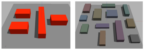
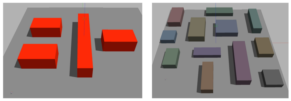
The first scenario contains several large obstacles separated by open passages, whereas the second contains more obstacles and narrower passages (Figure 6). Across both layouts, we compare route length, EDT corridor clearance, computation time, and task completion. The simulations use a two-dimensional planning grid; the indoor trials assess online map updating and route execution on the physical platform.

Figure 6. Representative simulation environments used for the UWB connectivity-aware navigation evaluation. The blue vertical lines indicate the vertical reference or measurement direction, while the green boxes denote the selected reference/target points.

The evaluation metrics were navigation success rate R, planning time $t_{\mathrm{plan}}$, trajectory optimization time $t_{\mathrm{opt}}$, normalized path length $L_{\mathrm{norm}}$, minimum EDT clearance $D_{min}$, mean EDT clearance $D_{\mathrm{mean}}$, velocity cost $c_v$, and acceleration cost $c_a$. A complete-navigation trial was successful when the method produced an executable route and the vehicle completed the start–goal task without collision; a path or trajectory-generation failure, collision, or incomplete task was counted as unsuccessful. For the trajectory-only comparison, success required generation of a collision-free executable trajectory for the supplied path. For each simulation condition, R is the number of successful tasks divided by ten; the tables report the corresponding completed/tested counts. Task completion and sampled clearance are evaluated as separate quantities. The trajectory-only comparison also reports execution duration $t_{\mathrm{exec}}=T_f$.

For a time-parameterized trajectory $x\left(t\right)$, the derivative costs are

$$c_v={\int }_0^{T_f}\parallel \dot{x}{\left(t\right)\parallel }_2^2\mathrm{d}t,c_a={\int }_0^{T_f}{\parallel \ddot{x}\left(t\right)\parallel }_2^2\mathrm{d}t.$$

(17)

For each successful task, m, let $J_m$ be the number of checked trajectory samples and define $D_{min}^{\left(m\right)}={min}_j{D}_t\left(q_j^{\left(m\right)}\right)$ and $D_{\mathrm{mean}}^{\left(m\right)}=J_m^{-1}{\sum }_{j=1}^{J_m}{D}_t\left(q_j^{\left(m\right)}\right)$ over those samples. The reported $D_{min}$ and $D_{\mathrm{mean}}$ are the per-task values averaged over successful tasks. The normalized path length is $L_{\mathrm{norm}}=L_{\mathrm{traj}}/{\parallel x_g-x_0\parallel }_2$, where $L_{\mathrm{traj}}$ is the generated route or trajectory length for the corresponding comparison. The units of $c_v$ and $c_a$ are ${\mathrm{m}}^2/\mathrm{s}$ and ${\mathrm{m}}^2/{\mathrm{s}}^3$, respectively. EDT values are sampled corridor measures rather than independently measured physical clearance along tracked flight. Consequently, $D_{min}$ and $D_{\mathrm{mean}}$ do not represent the actual minimum distance between the UAV body and an obstacle, and the present study does not use them as direct measurements of a physical safety margin. Timing, length, derivative-cost, and mean-clearance summaries are averages over successful tasks. The minimum EDT values are reported separately from the failure codes; failure-coded entries do not represent measured zero clearances. A dash excludes a failure-coded minimum from the distance statistics; it is not a measured zero clearance. Completion counts are reported separately. Because successful-task subsets differ between methods, their conditional averages are not paired estimates.

Values of $L_{\mathrm{norm}}$ close to one indicate a route close to the straight-line distance; larger values indicate a longer detour, which does not by itself establish greater clearance. The statistics describe the tested task sets and are interpreted descriptively. Table 1 lists the simulation settings and nominal motion limits.

Table 1. Simulation settings and nominal motion limits.

Parameter	Value
Workspace size	$50\mathrm{m}\times 50\mathrm{m}$
Grid resolution	$0.2\mathrm{m}$
Simulation framework	Gazebo, ROS, and RotorS Ardrone
Navigation tasks	10 start–goal pairs per scenario
Nominal available anchors	20
Nominal maximum velocity	$1.0\mathrm{m}/\mathrm{s}$
Nominal maximum acceleration	$2.0\mathrm{m}/{\mathrm{s}}^2$
Nominal maximum yaw rate	$1.2\mathrm{rad}/\mathrm{s}$

Common start and goal conditions control the task but do not establish equivalent sensing, map updates, or effective motion limits. The evaluation distinguishes whole-system execution, path selection on the corridor map, and trajectory generation from common discrete paths.

5.2. Comparison Methods

The EGO comparison uses a simplified EGO-style optimizer rather than a full reproduction of the original EGO-Planner. It receives the same connectivity-derived EDT grid representation through the optimizer interface and uses local B-spline-style optimization with EDT checking; the comparison is therefore reported as a descriptive reference configuration.

The comparison set was selected to cover both established planning primitives and a representative advanced UAV local planner. It includes a classical graph-search method, a classical optimization-based trajectory generator, a lightweight interpolation method, and a modern continuous local-optimization system. Table 2 summarizes their roles in the three evaluation levels.

Table 2. Roles of the comparison methods in the evaluation.

Method	Scientific Position and Principal Mechanism	Role in This Study
A* [20]	Classical graph search using a heuristic and distance-based accumulated cost	Path-planning comparator and front end of the system baseline
Minimum Snap [28]	Classical polynomial trajectory optimization using a high-order derivative cost	Back end of the system baseline and trajectory comparator
Piecewise Cubic Spline [35]	Lightweight segment-wise interpolation through discrete path points	Trajectory-generation comparator
EGO-style optimizer [31]	Advanced local planning using a B-spline and continuous gradient-based optimization	Complete-navigation system comparator

A*. A* is a classical deterministic graph-search algorithm that combines the accumulated cost from the start with a heuristic estimate to the goal [20]. It is widely used for grid-based robot path planning because it provides an efficient and reproducible reference when the search graph is fixed. In the reported comparison, the conventional A* planner uses path length as its accumulated objective and does not include the EDT clearance term. The reported A* and EDT-aware comparison uses the same connectivity-derived grid, neighborhood, and tasks, with the local EDT ranking term omitted for A*. This provides a component comparison within the stated formulation. A* also provides the route for the classical navigation baseline.

Minimum Snap. Minimum Snap is a classical trajectory-optimization method for quadrotors [28]. It represents each path segment by a polynomial and minimizes the integral of the squared snap while enforcing waypoint and inter-segment continuity constraints. The implementation uses seventh-order segment polynomials, continuity through jerk at internal waypoints, and zero endpoint derivatives. This method provides a conventional smoothness reference, but its objective does not explicitly encode the connectivity-derived EDT clearance. In the complete-navigation baseline, Minimum Snap converts the A* path into an executable trajectory. In the trajectory-only comparison, it receives exactly the same discrete point sequence as the other trajectory generators, allowing its smoothing behavior to be evaluated independently of path selection.

Piecewise Cubic Spline. Piecewise Cubic Spline (PCS) represents a lightweight interpolation-based alternative to optimization-heavy trajectory generation [35]. The implementation constructs segment-wise cubic curves through the supplied path points using endpoint and centered interior tangent estimates. PCS is computationally simple and preserves geometric continuity, making it a representative reference for direct path smoothing. However, it neither minimizes a high-order derivative objective nor includes an explicit EDT clearance term. PCS is used only in the trajectory-generation comparison, where all methods receive the same ten discrete paths and differ only in the back-end trajectory-generation procedure.

EGO-style optimizer (adapted from EGO-Planner). The tested EGO-style optimizer uses B-spline-based local trajectory optimization with EDT checking, following the general local-optimization role of EGO-Planner [31]. It is included as a complete-system reference rather than a path or trajectory ablation. The tested systems share scenarios, tasks, and nominal motion limits. The comparison describes the tested complete-system configurations; shared tasks are distinct from matched sensing and mapping inputs. The component comparisons separately examine path ranking and trajectory generation.

The path experiment holds the corridor map, neighborhood, tasks, and downstream processing fixed while changing path ranking. The trajectory experiment supplies ten common discrete paths to the back-end generators. Parameters were fixed across scenarios rather than retuned for individual tasks. These comparisons describe component behavior, but they do not form a full planning-by-refinement factorial design and cannot quantify a module-interaction effect. Table 3 summarizes the controls and interpretation of each comparison.

Table 3. Comparison controls and interpretation.

Comparison	Controlled Conditions	Comparison Scope
Path planning	Same corridor map, tasks, grid neighborhood; EDT ranking term varied	Local ranking comparison on the corridor map.
Trajectory generation	Ten common discrete input paths	Back-end comparison from common discrete paths.
Complete navigation	Same scenarios, tasks, nominal motion limits	Descriptive complete-system comparison; shared tasks do not imply matched sensing.

5.3. Connectivity-Degradation Protocol

The initial corridor is seeded by predefined anchor-to-anchor LOS edge sets. The connectivity study changes these configured edge sets (20, 15, and 10 available anchors), rather than injecting stochastic packet loss or classification errors.

To examine dependence on anchor availability, anchors were progressively removed from the simulated deployment while the environment, obstacle layout, start–goal tasks, and planning parameters were kept unchanged. The three conditions used 20, 15, and 10 available anchors, labeled Good, Moderate, and Poor, respectively. These labels identify the three tested configurations. The protocol varies anchor availability while retaining the geometry-based LOS/NLOS labeling procedure described in Section 5.1.

5.4. Platform and Trial Protocol

The five indoor anchors were placed at $(1,-4,0.7)$, $(0,0,0.7)$, $(-4,0,0.7)$, $(4,1,0.7)$, and $(1,4,0.7)$ m in the navigation frame; the UAV command altitude was fixed at $1.0$ m.

The system was also evaluated on a physical quadrotor in an $8\mathrm{m}\times 8\mathrm{m}$ indoor area containing cardboard and foam-box obstacles. The UAV was equipped with F100 2810 KV1100 motors (T-MOTOR, Nanchang, China), a Kakute H7 Mini flight controller (Holybro, Shenzhen, China), and an Intel NUC onboard computer with an Intel Core i7-1165G7 processor, 16 GB memory, and 500 GB storage. Nooploop LinkTrack P-B UWB modules provided ranging and localization observations. ROS hosted the perception, mapping, and planning nodes, while MAVLink connected the onboard computer to the flight controller.

UWB data followed two independent processing paths. UWB–IMU fusion with an unscented Kalman filter supplied the pose estimate, while a feature- and probability-distribution-based classifier supplied LOS/NLOS labels [16,19]. The navigation method treated these modules as inputs rather than contributions of the present paper. The $8\mathrm{m}\times 8\mathrm{m}$ workspace used a $0.2\mathrm{m}$ planning grid. Connectivity observations were processed at approximately 2 Hz. The system initialized the corridor from the connectivity available before flight, added LOS-supported cells online, recomputed the EDT field, and replanned after the UAV reached each local waypoint. The resulting trajectory was delivered through the ROS/MAVLink flight-control interface.

Five indoor start–goal trials were conducted. Success required completion of the assigned route without collision. Four trials completed, while Trial 3 did not. Section 6.5 presents the individual outcomes and computation times.

The indoor trials evaluate the complete processing chain: connectivity observations, corridor and EDT updates, trajectory generation, and delivery to the flight-control interface. They complement the simulation comparisons with execution on a physical platform.

5.5. Algorithm Parameters and Implementation Settings

The simulation settings and nominal motion limits are listed in Table 1. The indoor connectivity-processing loop runs at approximately 2 Hz and replanning follows arrival at a local waypoint; this rate describes software processing rather than the UWB device output rate. The comparison generators are described in Section 5.2. Table 4 provides the ten numerical settings for path ranking, sample correction, and time allocation, including their units and numerical stopping criteria.

Table 4. Algorithm parameters for path ranking, trajectory correction, and time allocation.

Parameter	Value	Meaning
$\lambda$	$0.04{\mathrm{m}}^2$	Weight of the local inverse-distance penalty in path ranking.
$\epsilon$	$1\times {10}^{-3}\mathrm{m}$	Regularizer in $1/(D+\epsilon )$.
$d_{\mathrm{safe}}$	$0.20\mathrm{m}$	Hard-sampled EDT threshold used by the trajectory implementation; not physical body clearance.
$\Delta t$	$0.02\mathrm{s}$	Controller period for trajectory commands and EDT statistics (50 Hz).
$v_{max}$	$1.0\mathrm{m}/\mathrm{s}$	Reference speed used in the turning-angle time-allocation rule.
$\alpha$	$1.0{\mathrm{rad}}^{-1}$	Sensitivity of local speed to the turning angle.
${\epsilon }_{\theta }$	$1\times {10}^{-8}{\mathrm{m}}^2$	Positive regularizer in the local turning-angle calculation.
$N_{\mathrm{iter}}$	20	Maximum EDT-guided refinement iterations; termination does not imply feasibility.
${\delta }_{\mathrm{ref}}$	$0.10\mathrm{m}$	Control-point correction step.
${\tau }_D$	$1\times {10}^{-3}\mathrm{m}$	Numerical tolerance for the sampled clearance check.

6. Results and Discussion

6.1. Navigation Performance Comparison

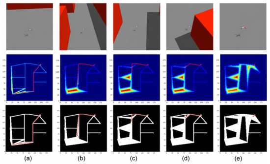
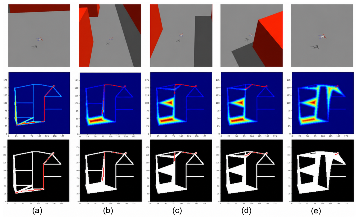
The system-level comparison evaluates complete task execution under the configurations described in Section 5.2. Figure 7 shows successive stages of simulated navigation. The first row presents the UAV view, the second the EDT field, and the third the corridor representation and planned route. The sequence records corridor expansion and route updates as LOS observations are accumulated during navigation. At the beginning, the UAV only has prior connectivity information between the UWB anchors, while the surrounding environment remains largely unknown. By establishing LOS connections with nearby anchors, the UAV gradually acquires information about the traversable regions and initializes the corresponding grid map and EDT distance field. As the UAV moves forward, the planner performs online path searching based on the currently available environmental representation. The generated path considers both path length and the safety cost derived from the EDT distance field, allowing the UAV to replan and switch paths during flight while maintaining a suitable safety margin. During navigation, LOS observations from different anchors are continuously incorporated into the map, and the EDT distance field is updated accordingly. As shown in panels (c,d), the planner dynamically adjusts the path as the environmental representation becomes more complete. Finally, in panel (e), the UAV reaches the target successfully. The traversable corridor gradually becomes connected, and the planned path evolves from an exploratory path into a smoother trajectory with a larger safety margin.

Figure 7. Representative simulated CoSafe-Nav navigation process from initial connectivity observations to completed route execution. The first row shows the UAV flight scenes, the second row presents the online-constructed EDT distance fields, and the third row shows the corresponding traversable corridors. The red curves denote the currently planned flight paths. Panels (a–e) show successive stages of the navigation process.

Table 5 compares the A*–Minimum Snap baseline, the adapted EGO-style optimizer, and CoSafe-Nav. CoSafe-Nav completed 10/10 tasks in both scenarios, compared with 6/10 and 5/10 for the baseline and 8/10 and 6/10 for the adapted EGO-style optimizer. Its positive minimum EDT values were 0.35 m and 0.30 m. Relative to the baseline, its mean planning time was higher by 0.008 s and 0.011 s, respectively, and its normalized path length was larger in both scenarios. These statistics describe the respective successful-task subsets.

Table 5. Comparison of complete navigation methods.

Metric	Baseline		EGO-Style		CoSafe-Nav
	S1	S2	S1	S2	S1	S2
Completed/tested	6/10	5/10	8/10	6/10	10/10	10/10
$t_{\mathrm{plan}}$ (s)	0.020	0.025	0.024	0.028	0.028	0.036
$t_{\mathrm{opt}}$ (s)	0.016	0.018	0.025	0.029	0.020	0.025
$D_{min}$ (m)	–	–	–	–	0.35	0.30
$D_{\mathrm{mean}}$ (m)	0.39	0.37	0.46	0.41	0.98	0.91
$L_{\mathrm{norm}}$	1.15	1.21	1.23	1.24	1.26	1.33
$c_v$ (${\mathrm{m}}^2/\mathrm{s}$)	5.03	5.00	2.37	2.38	3.94	4.03
$c_a$ (${\mathrm{m}}^2/{\mathrm{s}}^3$)	30.35	30.33	33.54	32.69	14.73	14.93

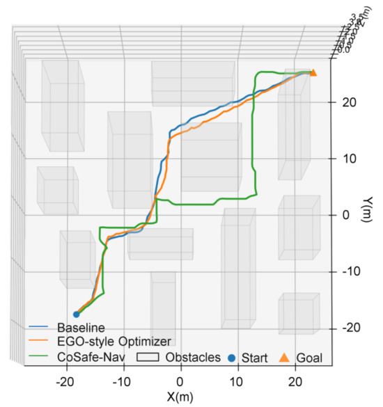
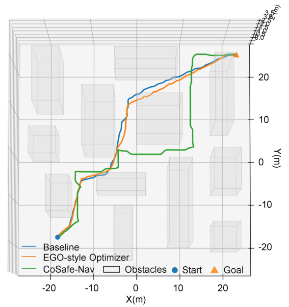
Figure 8 shows the trajectories of the three complete-navigation methods for a representative task. Gray solid shapes depict the simulator obstacles for visual context. The Baseline and EGO-style optimizer tend to generate relatively short routes through the environment; however, their trajectories pass close to obstacle boundaries in several local regions, leaving limited clearance and potentially increasing collision risk under modeling or tracking errors. In contrast, CoSafe-Nav follows a similar overall start-to-goal trend while maintaining a larger clearance from obstacles, resulting in a more outward-shifted trajectory near constrained regions. This behavior is attributed to the EDT-based safety cost, which penalizes low-clearance areas and encourages the trajectory to remain farther from obstacle boundaries. In narrow passages, CoSafe-Nav tends to follow the central region of the inferred traversable corridor, whereas the comparison methods more frequently approach the corridor boundaries. These observations provide qualitative evidence that the connectivity-derived corridor and EDT representation can support clearance-aware navigation.

Figure 8. Trajectory visualization for complete navigation methods in the perception-degraded environment.

Overall, the results indicate that the proposed corridor-guided processing chain is able to update the traversable representation online and generate executable routes for the tested task sets. CoSafe-Nav completed all tested tasks in both simulation scenarios, while also producing paths with greater conditional EDT clearance and longer normalized path length. These results support the feasibility of combining connectivity-derived corridor construction with EDT-aware navigation under the tested conditions, but they do not establish overall superiority over the baselines because the systems did not use fully matched sensing and mapping inputs. The following subsections therefore interpret path planning and trajectory generation separately; all continuous metrics are conditional on successful completion.

6.2. Path-Planning Comparison

The path comparison changes the local EDT ranking term while keeping the corridor map, tasks, neighborhood, and downstream processing fixed. Completion is an outcome of the evaluated pipeline; differences in completion counts do not imply that the ranking term changes the reachability of a fixed search graph.

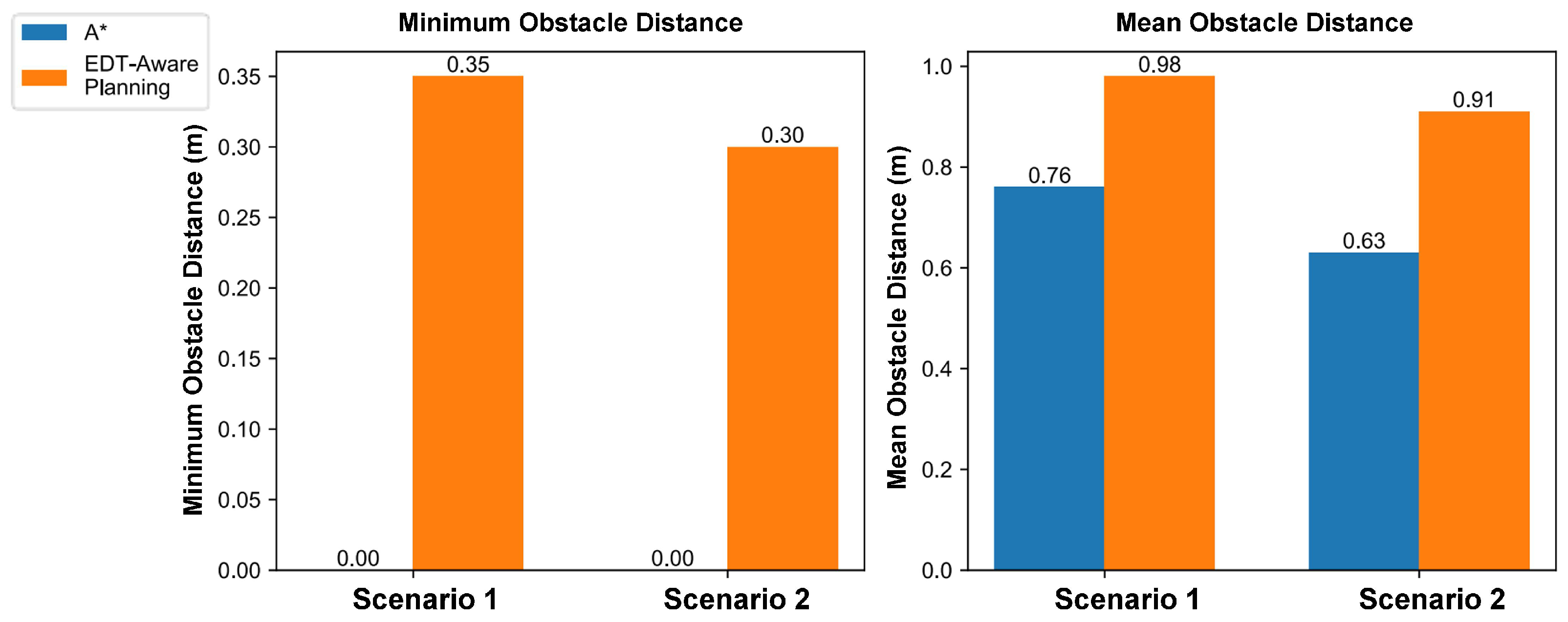
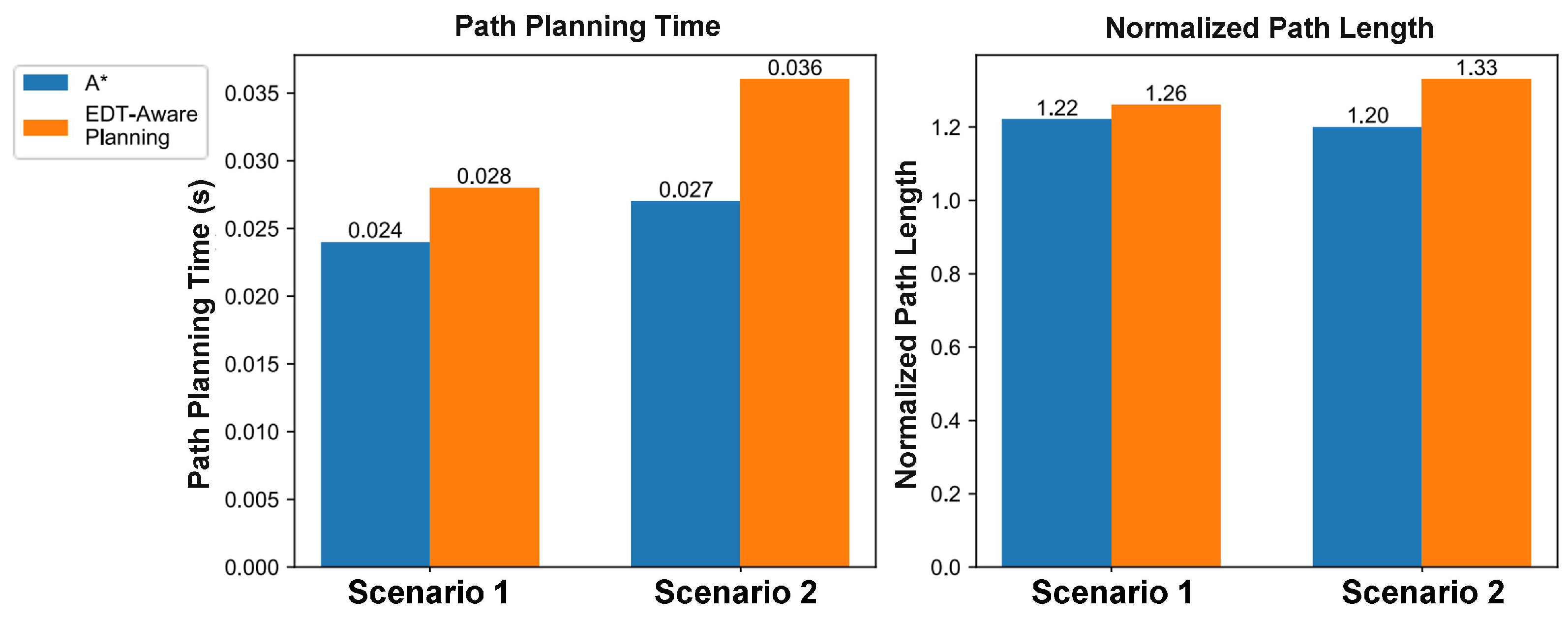
Table 6 compares A* and EDT-aware planning. EDT-aware planning completed 10/10 tasks in both scenarios, compared with 7/10 and 6/10 for A*. Mean EDT clearance was 0.98 m versus 0.76 m in S1 and 0.91 m versus 0.63 m in S2. Planning time increased by 0.004 s and 0.009 s, respectively. The higher conditional corridor-clearance means were accompanied by longer normalized paths.

Table 6. Comparison of A* and EDT-Aware Planning.

Method	Scene	Trials	${\mathit{t}}_{\mathbf{plan}}$ (s)	${\mathit{L}}_{\mathbf{norm}}$	${\mathit{D}}_{min}$ (m)	${\mathit{D}}_{\mathbf{mean}}$ (m)
A*	S1	7/10	0.024	1.22	–	0.76
A*	S2	6/10	0.027	1.20	–	0.63
EDT-Aware Planning	S1	10/10	0.028	1.26	0.35	0.98
EDT-Aware Planning	S2	10/10	0.036	1.33	0.30	0.91

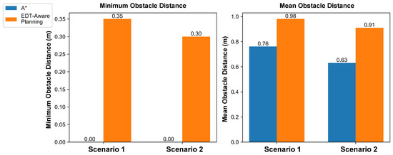
Figure 9 presents EDT corridor-clearance summaries. Its zero minimum entries encode failure and are excluded from clearance interpretation; Table 6 separates these entries from measured distances using dashes and reports task completion explicitly. Mean clearances describe each method’s successful tasks, so the comparison is descriptive across the tested task sets.

Figure 9. Path-planning clearance comparison. The in-figure labels “Minimum Obstacle Distance” and “Mean Obstacle Distance” denote EDT corridor-clearance summaries in meters, measured to unsupported grid cells, rather than physical obstacle or UAV-body clearance. The A* minimum entries labeled 0.00 are failure codes, not measured zero clearances; they correspond to dashes in Table 6. Mean values summarize successful tasks. Completion counts are reported separately in Table 6: 7/10 and 6/10 for A*, and 10/10 in each scenario for EDT-aware planning.

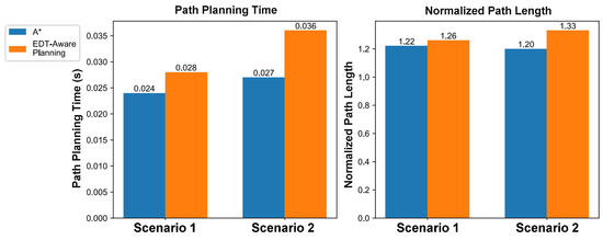
Figure 10 reports the corresponding increases in planning time and normalized path length. Together, these summaries describe the observed trade-off between corridor clearance, route length, and planning time.

Figure 10. Efficiency comparison between A* and EDT-Aware Planning.

Overall, the component comparison indicates that adding the EDT-based local ranking term improved the conditional corridor clearance and task-completion results in the tested scenarios. This improvement was accompanied by modest increases in planning time and normalized path length, which supports the usefulness of the EDT term for clearance-aware path selection under the evaluated corridor representation.

6.3. Trajectory-Generation Comparison

The trajectory comparison evaluates whether the clearance preference is preserved when identical discrete paths are converted into executable trajectories.

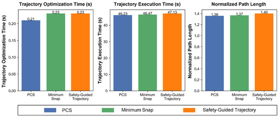
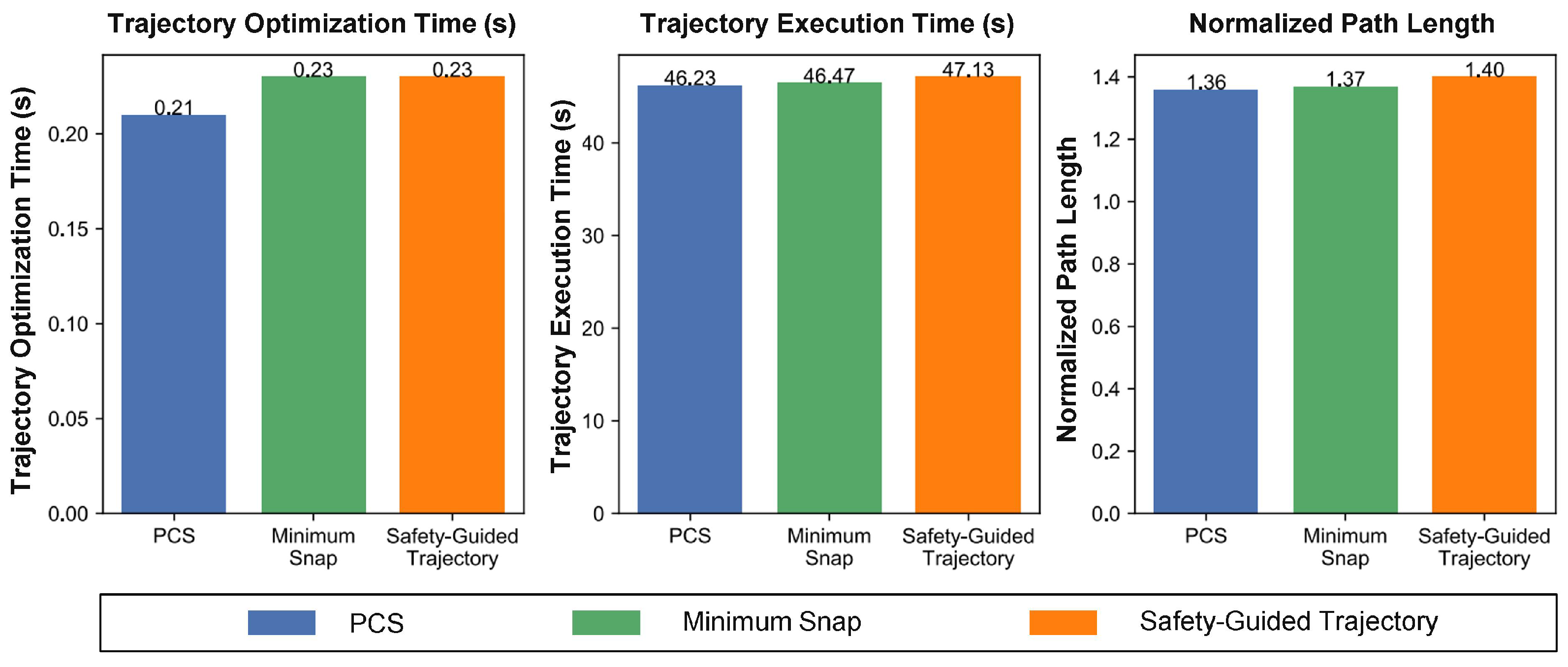
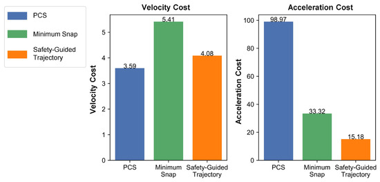
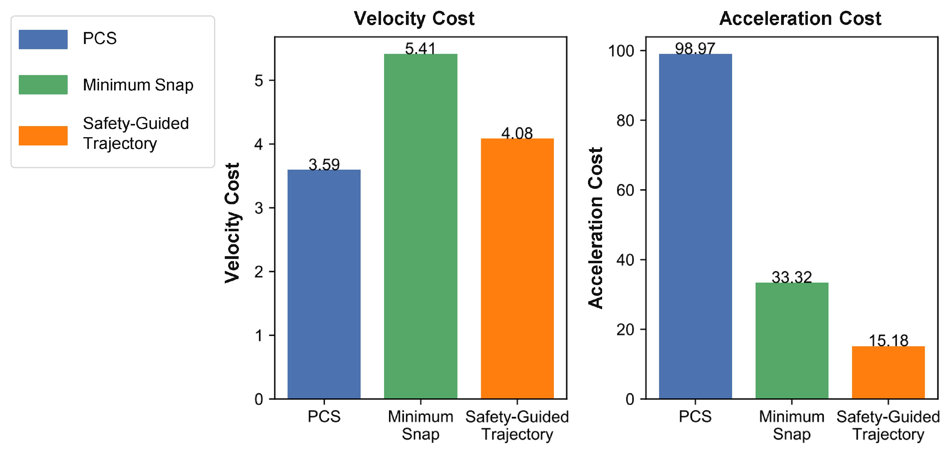
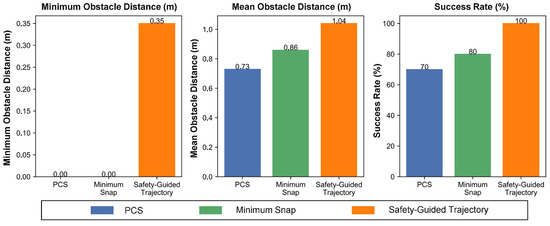
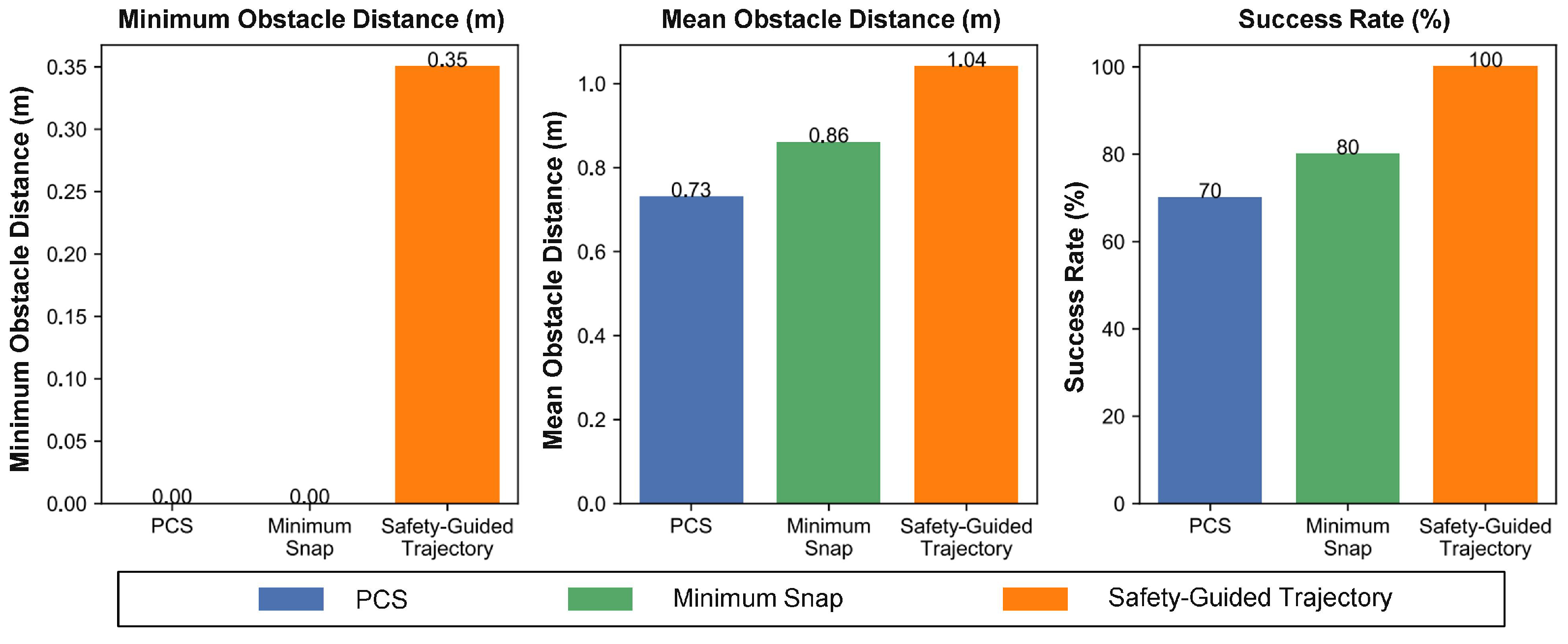
The safety-guided method completed 10/10 trajectory tasks, compared with 7/10 for piecewise cubic spline and 8/10 for Minimum Snap. Among successful trajectories, its mean EDT clearance was 1.04 m, compared with 0.73 m and 0.86 m, and its acceleration integral was 15.18 ${\mathrm{m}}^2/{\mathrm{s}}^3$, compared with 98.97 and 33.32 ${\mathrm{m}}^2/{\mathrm{s}}^3$. These conditional summaries describe the tested trajectory inputs and should not be interpreted as estimates of general performance. The safety-guided method also produced the largest normalized path length (1.40) and longest mean execution duration (47.13 s). Its lower acceleration integral and greater corridor clearance therefore accompany changes in route length and timing. The experiment does not separate the contribution of spatial correction from that of time allocation.

Figure 11 compares optimization time, execution duration, and normalized path length. The mean optimization times range from 0.21 to 0.23 s in this trajectory-only comparison. They should not be equated with the shorter optimization calls in the complete-navigation comparison, which uses different trajectory inputs.

Figure 11. Efficiency comparison of piecewise cubic spline, Minimum Snap, and safety-guided trajectory generation.

Figure 12 compares the derivative integrals. The safety-guided method has the lowest acceleration integral, while its velocity integral lies between the two references. These measures summarize temporal variation over a trajectory and are distinct from peak velocity and acceleration.

Figure 12. Derivative-integral comparison for trajectory generation. “Velocity Cost” denotes ${\int }_0^{T_f}{\parallel \dot{x}\left(t\right)\parallel }_2^{2}dt$ in ${\mathrm{m}}^2/\mathrm{s}$, and “Acceleration Cost” denotes ${\int }_0^{T_f}{\parallel \ddot{x}\left(t\right)\parallel }_2^{2}dt$ in ${\mathrm{m}}^2/{\mathrm{s}}^3$. PCS denotes piecewise cubic spline. These integral metrics are distinct from peak velocity and acceleration.

Figure 13 presents EDT corridor-clearance summaries and success rates. The zero minimum entries are failure codes, while the positive minimum and mean values are corridor-clearance summaries. Table 7 uses dashes for failure-coded minima and expresses completion as completed/tested counts.

Figure 13. Trajectory-generation clearance and completion comparison. The in-figure “Obstacle Distance” labels denote EDT corridor clearance in meters, not physical obstacle or UAV-body clearance. The 0.00 minimum entries for PCS and Minimum Snap encode failed tasks and correspond to dashes in Table 7; they are not measured zero clearances. Mean values summarize successful tasks. Success rates of 70%, 80%, and 100% correspond to 7/10, 8/10, and 10/10 completed tasks, respectively. PCS denotes piecewise cubic spline.

Table 7. Comparison of trajectory-generation methods.

Metric	Piecewise Cubic Spline	Minimum Snap	Safety-Guided Trajectory
Completed/tested	7/10	8/10	10/10
$t_{\mathrm{opt}}$ (s)	0.21	0.23	0.23
$t_{\mathrm{exec}}$ (s)	46.23	46.47	47.13
$L_{\mathrm{norm}}$	1.36	1.37	1.40
$c_v$ (${\mathrm{m}}^2/\mathrm{s}$)	3.59	5.41	4.08
$c_a$ (${\mathrm{m}}^2/{\mathrm{s}}^3$)	98.97	33.32	15.18
$D_{min}$ (m)	–	–	0.35
$D_{\mathrm{mean}}$ (m)	0.73	0.86	1.04

6.4. Effect of UWB Connectivity

The connectivity analysis varies the configured anchor availability while keeping the planning procedure and geometry-based LOS labeling unchanged. Table 8 reports 4/10, 9/10, and 10/10 completed tasks for deployments with 10, 15, and 20 available anchors. Their mean EDT clearances were 0.61, 0.68, and 0.91 m, respectively. Normalized path lengths of 1.35, 1.39, and 1.33 show no monotonic trend. These results characterize the tested deployments rather than a universal anchor-count threshold.

Table 8. Navigation performance under different UWB connectivity conditions.

Metric	Poor	Moderate	Good
Available anchors	10	15	20
Completed/tested	4/10	9/10	10/10
$t_{\mathrm{plan}}$ (s)	0.028	0.033	0.036
$D_{min}$ (m)	–	0.20	0.30
$D_{\mathrm{mean}}$ (m)	0.61	0.68	0.91
$L_{\mathrm{norm}}$	1.35	1.39	1.33

Across the three tested configurations, the 20-anchor deployment had the highest completion count and mean EDT corridor clearance. The normalized path length was highest for the 15-anchor deployment. These observations describe the configurations in Table 8; anchor count is the varied experimental factor, while corridor coverage is not a separately measured metric. The anchor-removal comparison concerns observation availability under the fixed geometry-based labeling procedure. Controlled classification errors, packet loss, and observation delay are addressed in the future work in Section 6.6.

Taken together, these results indicate that anchor availability is an important factor affecting the completeness of the inferred traversable corridor and the reliability of navigation. More available anchors generally provide broader connectivity observations, leading to higher task-completion rates and greater mean EDT clearance. However, the normalized path length does not vary monotonically with anchor count, indicating that connectivity availability affects route selection through changes in corridor structure rather than simply determining the path length.

6.5. Indoor UAV Platform Validation

The indoor-platform evaluation records task completion, planning and optimization times, and successive flight and map-update states. Of the five indoor trials, four were successfully completed, as summarized in Table 9. Planning times for the completed trials ranged from 0.003 to 0.008 s and trajectory optimization times from 0.008 to 0.020 s. Trial 3 was incomplete. Table 9 summarizes the task outcomes and computation times for the completed trials.

Table 9. Indoor task outcomes and computation times. Dashes indicate an incomplete trial rather than measured zero computation times.

Trial	Completed	${\mathit{t}}_{\mathbf{plan}}$ (s)	${\mathit{t}}_{\mathbf{opt}}$ (s)
1	Yes	0.008	0.020
2	Yes	0.003	0.008
3	No	–	–
4	Yes	0.004	0.009
5	Yes	0.006	0.010

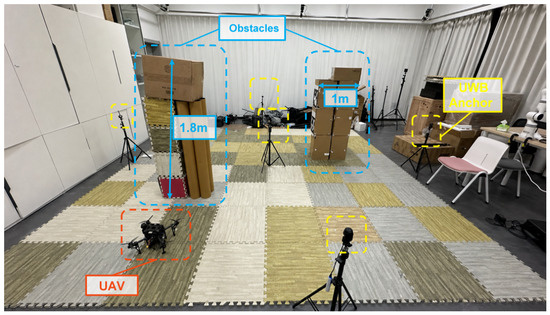
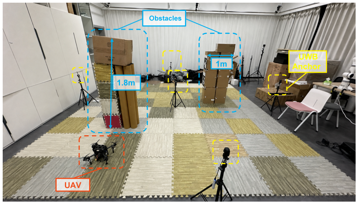
Figure 14 shows the physical environment used for indoor platform validation. The obstacles form open passages together with locally constrained regions, and the deployed UWB anchors provide the connectivity observations required by the proposed navigation system. The annotations identify the UAV and representative anchors and mark an obstacle height of 1.8 m and a horizontal obstacle dimension of 1 m. Both dimensions refer to the depicted obstacle geometry.

Figure 14. Indoor UAV validation scenario with obstacles and deployed UWB anchors.

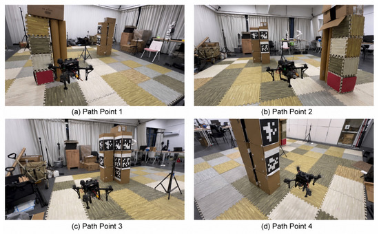
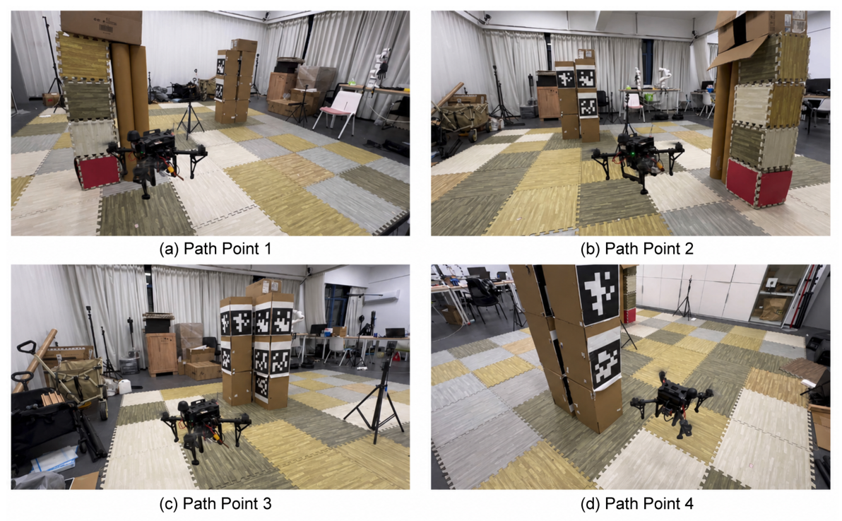
Figure 15 records four successive UAV states from a representative successful trial. The panels correspond to Path Points 1–4 and show the vehicle progressing through different parts of the obstacle layout as the local waypoints are reached. The sequence shows route execution in the physical environment alongside the per-trial outcomes in Table 9.

Figure 15. Representative flight states of the UAV at successive route points during indoor validation.

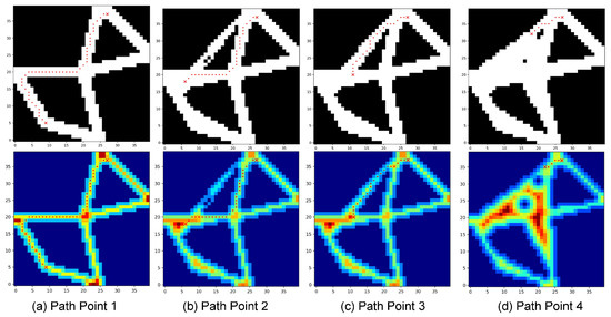
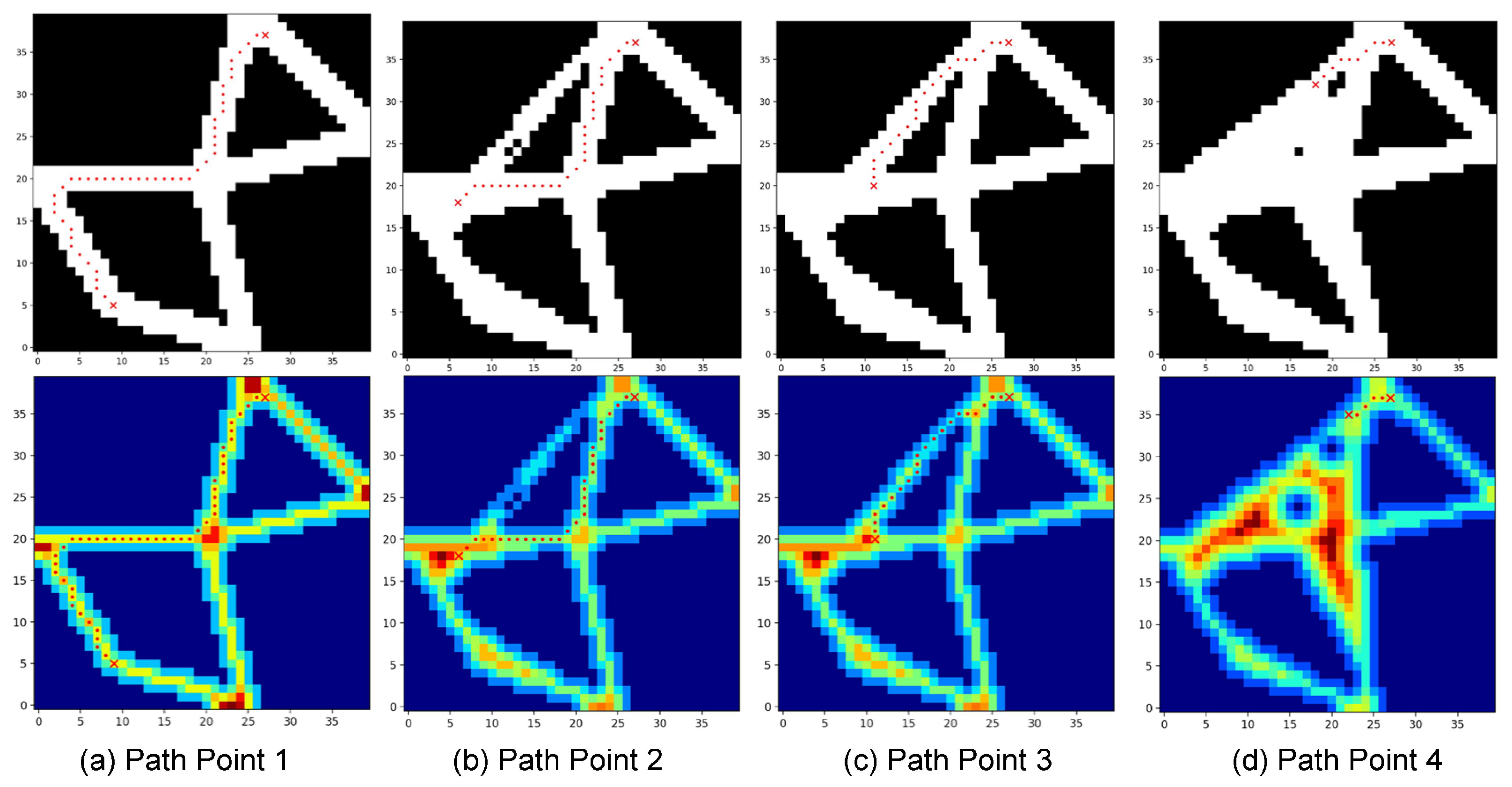
Figure 16 presents the connectivity-derived binary corridor map and the corresponding EDT field at the same four path points. As additional UWB link-state observations are accumulated, the supported traversable region develops from a relatively sparse structure into a more complete corridor representation. The EDT field is recomputed from the updated binary map, and the displayed route is consequently updated using the evidence available at each path point. The four panels show successive corridor, EDT, and route updates during the trial.

Figure 16. Evolution of the binary corridor map and EDT field during indoor UAV navigation. The color variations in the EDT maps represent different EDT values, with blue-to-red colors indicating increasing distance to unsupported grid-cell centers. The red dotted curves denote the planned paths, and the red crosses indicate the path endpoints and selected intermediate waypoints.

The simulation and flight sequences provide qualitative evidence of incremental map updating and route execution. Together with the component comparisons, they characterize operation of the integrated pipeline under the stated tasks and deployment conditions. Overall, the indoor trials demonstrate the practical feasibility of the proposed connectivity-aware navigation pipeline, including online corridor updating, EDT reconstruction, path replanning, and flight-control execution. However, the limited number of trials provides feasibility evidence rather than a statistically conclusive validation of general performance.

6.6. Scope and Future Work

The applicable setting requires pre-deployed anchors with known coordinates, an available pose estimate, and fixed-altitude planar motion. The pose and classification modules are inputs to the planner. The indoor platform and anchor arrangement are described in Section 5.4 and illustrated in Figure 14. The reported corridor-clearance metric belongs to the grid representation, whereas physical body clearance is a distinct quantity. An actual minimum obstacle clearance for the executed trajectories would require synchronized trajectory data, obstacle geometry, and an airframe footprint. These quantities are not evaluated in the present study; therefore, physical body-clearance validation remains a limitation and a priority for future work.

An inferred corridor represents accumulated LOS support. Under the monotonic update, a cell added by a false LOS label remains supported for the mission, while NLOS and unavailable observations add no cells. This behavior follows the update rule in Section 4.1. The simulation uses geometry-based labels, and the anchor-removal comparison varies their availability. Classification errors, packet loss, observation delay, and changing obstacles define further evaluation conditions.

The study contains two simulation task sets of ten tasks each and five indoor trials. Completion is reported as counts, and continuous metrics summarize successful tasks within each configuration. Different successful subsets make these descriptive summaries distinct from paired estimates. The conclusions apply to the tested task sets and deployment conditions.

Future work will prioritize independent corridor-coverage and false-free-cell evaluation, body-aware obstacle-clearance measurements, and controlled tests of LOS and NLOS classification errors, packet loss, and observation delay. Confidence-weighted reversible updates will be investigated to address persistent false support. Future evaluation will also measure final trajectory peaks and swept-volume clearance. A matched-input EGO-Planner comparison and a planning-by-refinement factorial study will separate system and module effects. Larger task sets with recorded seeds, complete configurations, and synchronized flight logs will support uncertainty analysis and failure diagnosis.

7. Conclusions

CoSafe-Nav connects sparse UWB link observations to route execution through an inferred corridor and a shared EDT representation. In the tested planar settings, it completed 10/10 navigation tasks in each simulation scenario and four of five indoor trials. The component comparisons show greater conditional mean corridor clearance with longer routes, and a lower acceleration integral for safety-guided trajectory generation. These observations support the feasibility of the integrated processing chain under the stated deployment assumptions.

The findings concern fixed-altitude planar navigation with pre-deployed anchors and the task sets evaluated in this study. The EDT represents grid-based corridor clearance, while the timing rule allocates segment durations and the derivative integrals summarize trajectory variation. The reported EDT values should therefore be interpreted as sampled corridor-clearance measures rather than actual physical safety margins. Future work will evaluate physical body clearance and radio errors, measure continuous-trajectory extrema, and extend controlled comparisons to larger task sets.

References

- He, B.; Ji, X.; Li, G.; Cheng, B. Key technologies and applications of UAVs in underground space: A review. IEEE Trans. Cogn. Commun. Netw. 2024, 10, 1026–1049. [Google Scholar] [CrossRef] [Scilit]
- Idrissi, M.; Salami, M.; Annaz, F. A review of quadrotor unmanned aerial vehicles: Applications, architectural design and control algorithms. J. Intell. Robot. Syst. 2022, 104, 22. [Google Scholar] [CrossRef] [Scilit]
- Uddin, Z.; Dindar, S. A drone-integrated safety framework for sustainable rail infrastructure management and accident prevention. Sci. J. Silesian Univ. Technol. Ser. Transp. 2026, 130, 235–256. [Google Scholar] [CrossRef] [Scilit]
- Coppens, D.; Shahid, A.; Lemey, S.; Van Herbruggen, B.; Marshall, C.; De Poorter, E. An overview of UWB standards and organizations (IEEE 802.15.4, FiRa, Apple): Interoperability aspects and future research directions. IEEE Access 2022, 10, 70219–70241. [Google Scholar] [CrossRef] [Scilit]
- Kao, P.-Y.; Chang, H.-J.; Tseng, K.-W.; Chen, T.; Luo, H.-L.; Hung, Y.-P. VIUNet: Deep visual–inertial–UWB fusion for indoor UAV localization. IEEE Access 2023, 11, 61525–61534. [Google Scholar] [CrossRef] [Scilit]
- Zeng, Q.; Jin, Y.; Yu, H.; You, X. A UAV localization system based on double UWB tags and IMU for landing platform. IEEE Sens. J. 2023, 23, 10100–10108. [Google Scholar] [CrossRef] [Scilit]
- Zheng, S.; Li, Z.; Liu, Y.; Zhang, H.; Zheng, P.; Liang, X.; Li, Y.; Bu, X.; Zou, X. UWB-VIO fusion for accurate and robust relative localization of round robotic teams. IEEE Robot. Autom. Lett. 2022, 7, 11950–11957. [Google Scholar] [CrossRef] [Scilit]
- Zafari, F.; Gkelias, A.; Leung, K.K. A survey of indoor localization systems and technologies. IEEE Commun. Surv. Tutor. 2019, 21, 2568–2599. [Google Scholar] [CrossRef] [Scilit]
- Mur-Artal, R.; Montiel, J.M.M.; Tardos, J.D. ORB-SLAM: A versatile and accurate monocular SLAM system. IEEE Trans. Robot. 2015, 31, 1147–1163. [Google Scholar] [CrossRef] [Scilit]
- Campos, C.; Elvira, R.; Rodríguez, J.J.G.; Montiel, J.M.M.; Tardós, J.D. ORB-SLAM3: An accurate open-source library for visual, visual–inertial, and multimap SLAM. IEEE Trans. Robot. 2021, 37, 1874–1890. [Google Scholar] [CrossRef] [Scilit]
- Qin, T.; Li, P.; Shen, S. VINS-Mono: A robust and versatile monocular visual-inertial state estimator. IEEE Trans. Robot. 2018, 34, 1004–1020. [Google Scholar] [CrossRef] [Scilit]
- Zhang, J.; Singh, S. LOAM: Lidar odometry and mapping in real-time. In Proceedings of the Robotics: Science and Systems X, Berkeley, CA, USA, 12–16 July 2014. [Google Scholar] [CrossRef] [Scilit]
- Xu, W.; Zhang, F. FAST-LIO: A fast, robust LiDAR-inertial odometry package by tightly-coupled iterated Kalman filter. IEEE Robot. Autom. Lett. 2021, 6, 3317–3324. [Google Scholar] [CrossRef] [Scilit]
- Xu, W.; Cai, Y.; He, D.; Lin, J.; Zhang, F. FAST-LIO2: Fast direct lidar-inertial odometry. IEEE Trans. Robot. 2022, 38, 2053–2073. [Google Scholar] [CrossRef] [Scilit]
- Zheng, C.; Zhu, Q.; Xu, W.; Liu, X.; Guo, Q.; Zhang, F. FAST-LIVO: Fast and tightly-coupled sparse-direct lidar-inertial-visual odometry. In Proceedings of the 2022 IEEE/RSJ International Conference on Intelligent Robots and Systems, Kyoto, Japan, 23–27 October 2022; pp. 4003–4009. [Google Scholar] [CrossRef] [Scilit]
- Che, F.; Ahmed, Q.Z.; Fontaine, J.; Van Herbruggen, B.; Shahid, A.; De Poorter, E.; Lazaridis, P.I. Feature-based generalized Gaussian distribution method for NLOS detection in ultra-wideband indoor positioning system. IEEE Sens. J. 2022, 22, 18726–18739. [Google Scholar] [CrossRef] [Scilit]
- Yang, H.; Wang, Y.; Seow, C.K.; Sun, M.; Si, M.; Huang, L. UWB sensor-based indoor LOS/NLOS localization with support vector machine learning. IEEE Sens. J. 2023, 23, 2988–3004. [Google Scholar] [CrossRef] [Scilit]
- Yang, H.; Wang, Y.; Seow, C.K.; Sun, M.; Coene, S.; Huang, L.; Joseph, W.; Plets, D. Fuzzy transformer machine learning for UWB NLOS identification and ranging mitigation. IEEE Trans. Instrum. Meas. 2025, 74, 8503817. [Google Scholar] [CrossRef] [Scilit]
- You, W.; Li, F.; Liao, L.; Huang, M. Data fusion of UWB and IMU based on unscented Kalman filter for indoor localization of quadrotor UAV. IEEE Access 2020, 8, 64971–64981. [Google Scholar] [CrossRef] [Scilit]
- Hart, P.E.; Nilsson, N.J.; Raphael, B. A formal basis for the heuristic determination of minimum cost paths. IEEE Trans. Syst. Sci. Cybern. 1968, 4, 100–107. [Google Scholar] [CrossRef] [Scilit]
- Koenig, S.; Likhachev, M. D* Lite. In Proceedings of the Eighteenth National Conference on Artificial Intelligence, Edmonton, AB, Canada, 28 July–1 August 2002; AAAI Press: Menlo Park, CA, USA, 2002; pp. 476–483. [Google Scholar]
- LaValle, S.M.; Kuffner, J.J., Jr. Rapidly-exploring random trees: Progress and prospects. In Algorithmic and Computational Robotics: New Directions; Donald, B.R., Lynch, K.M., Rus, D., Eds.; A K Peters: Wellesley, MA, USA, 2001; pp. 293–308. [Google Scholar]
- Karaman, S.; Frazzoli, E. Sampling-based algorithms for optimal motion planning. Int. J. Robot. Res. 2011, 30, 846–894. [Google Scholar] [CrossRef] [Scilit]
- Gammell, J.D.; Srinivasa, S.S.; Barfoot, T.D. Informed RRT*: Optimal sampling-based path planning focused via direct sampling of an admissible ellipsoidal heuristic. In Proceedings of the 2014 IEEE/RSJ International Conference on Intelligent Robots and Systems, Chicago, IL, USA, 14–18 September 2014; pp. 2997–3004. [Google Scholar] [CrossRef] [Scilit]
- Elfes, A. Occupancy grids: A stochastic spatial representation for active robot perception. In Proceedings of the Sixth Conference on Uncertainty in Artificial Intelligence, Cambridge, MA, USA, 27–29 July 1990; Morgan Kaufmann: San Francisco, CA, USA, 1990; pp. 136–146. [Google Scholar]
- Oleynikova, H.; Taylor, Z.; Fehr, M.; Siegwart, R.; Nieto, J. Voxblox: Incremental 3D Euclidean signed distance fields for on-board MAV planning. In Proceedings of the 2017 IEEE/RSJ International Conference on Intelligent Robots and Systems, Vancouver, BC, Canada, 24–28 September 2017; pp. 1366–1373. [Google Scholar] [CrossRef] [Scilit]
- Han, L.; Gao, F.; Zhou, B.; Pan, J.; Shen, S. FIESTA: Fast incremental Euclidean distance fields for online motion planning of aerial robots. In Proceedings of the 2019 IEEE/RSJ International Conference on Intelligent Robots and Systems, Macau, China, 3–8 November 2019; pp. 4423–4430. [Google Scholar] [CrossRef] [Scilit]
- Mellinger, D.; Kumar, V. Minimum snap trajectory generation and control for quadrotors. In Proceedings of the 2011 IEEE International Conference on Robotics and Automation, Shanghai, China, 9–13 May 2011; pp. 2520–2525. [Google Scholar] [CrossRef] [Scilit]
- Richter, C.; Bry, A.; Roy, N. Polynomial trajectory planning for aggressive quadrotor flight in dense indoor environments. In Robotics Research; Inaba, M., Corke, P., Eds.; Springer: Cham, Switzerland, 2016; Volume 114, pp. 649–666. [Google Scholar] [CrossRef] [Scilit]
- Usenko, V.; von Stumberg, L.; Pangercic, A.; Cremers, D. Real-time trajectory replanning for MAVs using uniform B-splines and a 3D circular buffer. In Proceedings of the 2017 IEEE/RSJ International Conference on Intelligent Robots and Systems, Vancouver, BC, Canada, 24–28 September 2017; pp. 215–222. [Google Scholar] [CrossRef] [Scilit]
- Zhou, X.; Wang, Z.; Ye, H.; Xu, C.; Gao, F. EGO-Planner: An ESDF-free gradient-based local planner for quadrotors. IEEE Robot. Autom. Lett. 2021, 6, 478–485. [Google Scholar] [CrossRef] [Scilit]
- Tordesillas, J.; Lopez, B.T.; How, J.P. FASTER: Fast and safe trajectory planner for flights in unknown environments. In Proceedings of the 2019 IEEE/RSJ International Conference on Intelligent Robots and Systems, Macau, China, 3–8 November 2019; pp. 1934–1940. [Google Scholar] [CrossRef] [Scilit]
- Liu, S.; Watterson, M.; Mohta, K.; Sun, K.; Bhattacharya, S.; Taylor, C.J.; Kumar, V. Planning dynamically feasible trajectories for quadrotors using safe flight corridors in 3-D complex environments. IEEE Robot. Autom. Lett. 2017, 2, 1688–1695. [Google Scholar] [CrossRef] [Scilit]
- Ji, J.; Zhou, X.; Xu, C.; Gao, F. CMPCC: Corridor-based model predictive contouring control for aggressive drone flight. In Experimental Robotics; Springer: Cham, Switzerland, 2021; Volume 19, pp. 37–46. [Google Scholar] [CrossRef] [Scilit]
- de Boor, C. A Practical Guide to Splines; Applied Mathematical Sciences; Springer: New York, NY, USA, 2001; Volume 27. [Google Scholar]
Disclaimer/Publisher’s Note: The statements, opinions and data contained in all publications are solely those of the individual author(s) and contributor(s) and not of MDPI and/or the editor(s). MDPI and/or the editor(s) disclaim responsibility for any injury to people or property resulting from any ideas, methods, instructions or products referred to in the content. |
© 2026 by the authors. Licensee MDPI, Basel, Switzerland. This article is an open access article distributed under the terms and conditions of the Creative Commons Attribution (CC BY) license.