


Abstract
An exploratory equivalent partition (EE partition) of a graph G with nontrivial automorphisms is a partition of its vertex set that can be directly translated into a set of constraints to speed up the search for occurrences of G in an arbitrary host graph. The maximum EE partition problem is to find an EE partition leading to the greatest speedup. However, this problem is NP-hard and the naïve algorithm is only practicable for small symmetry-rich graphs. In this paper, we propose a series of improvements based on computational group theory that vastly increase the algorithm’s range of practicability. For example, the improved algorithm spends less time on the 10-hypercube graph (1024 vertices, 5120 edges, ≈3.7 × 10⁹ automorphisms) than the naïve algorithm does on the 4-hypercube graph (16 vertices, 32 edges, 384 automorphisms). We prove that all improvements maintain the algorithm’s correctness and confirm their contribution to the speed of execution through extensive experimentation.
1. Introduction
In the era of networks of all possible types and sizes, the graph is one of the most important mathematical and computational structures. A fundamental problem associated with graphs is that of subgraph isomorphism search: given a (smaller) pattern graph G and a (larger) host graph H, report one (or all, depending on the definition) of the occurrences of G in H. This problem has found applications in computer science [1], social sciences [2], chemistry [3], logistics [4], etc.
Unfortunately, the subgraph isomorphism problem is NP-hard, implying that an efficient (polynomial-time) algorithm is unlikely to exist. In practice, some approaches do perform reasonably well for most graphs of moderate size, but may falter when the pattern graph has many symmetries (automorphisms) [5,6]. For this reason, we [7,8] defined an equivalence relation on graph vertices called exploratory equivalence. Exploratory equivalence induces an exploratory equivalent partition (or EE partition) of the graph vertex set, which can be readily translated into a set of constraints that can be employed during the execution of any subgraph isomorphism search algorithm. Those constraints may significantly improve performance; in particular, if they are applied to an algorithm that is oblivious to the symmetries of the pattern graph, they reduce the number of established vertex-to-vertex correspondences between the pattern graph and the host graph by the product of the factorials of the sizes of the equivalence classes constituting the partition. This product is called the score of the EE partition.
A given graph may have multiple EE partitions, each with its own score. Of particular interest is an EE partition with the greatest score—a maximum EE partition. (Since there may be multiple maximum EE partitions, we speak of a rather than the maximum EE partition.) Such a partition can be converted into a set of constraints that improves the performance of subgraph isomorphism search by the greatest factor.
Unsurprisingly, the problem of finding a maximum EE partition (MaxEE) is itself hard [8]. In particular, we showed that the associated verification problem (given a graph and a partition, verify that the partition is an EE partition of that graph) is at least as hard as the graph isomorphism problem and at most as hard as the set stabilizer problem, which places the verification problem between the complexity classes P and NP. This means that the decision version of the optimization problem (given a graph and an integer k, determine whether there is an EE partition with a score greater than k) is not known to be in NP, and the optimization problem itself (given a graph, report one of its maximum EE partitions) is not known to be in FNP (Function NP). In other words, it is at least as hard as the hardest problems in FNP (such as the subgraph isomorphism problem) but may, in fact, be strictly harder.
Facing the inherent hardness of the MaxEE problem, there are a few possible directions as to where to steer our research. One possibility is to focus on restricted classes of graphs, such as trees, cycles, or complete graphs. It turns out that, for some classes, the MaxEE problem can be solved in polynomial time, or it may even have a closed-form solution [9]. Another option is to seek an efficient heuristic approach. We proposed an efficient (although theoretically still superpolynomial) suboptimal algorithm and showed that it finds an optimal solution for a majority of graphs, although in some cases, the score of the discovered EE partition could arbitrarily diverge from the maximum [8].
In this paper, we take a third route. We present a novel algorithm that finds a maximum EE partition for an arbitrary graph in a highly efficient manner. Naturally, we could not escape exponential behavior for some classes of graphs, but we were nevertheless able to improve the performance significantly; for example, the time spent by the naïve algorithm (one that follows the definition of a maximum EE partition) on the 4-hypercube graph (16 vertices, 32 edges, and 384 automorphisms) is longer than the time spent by the improved algorithm on the 10-hypercube graph (1024 vertices, 5120 edges, and ≈3.7 × 10⁹ automorphisms).
The contribution of this paper is thus of a practical rather than theoretical nature. In particular, while the worst-case complexity of the algorithm remains exponential in terms of the input graph size, our experiments showed a considerable improvement of its execution time on several symmetry-rich graph families. In the process of devising an improved algorithm, we heavily relied on results from computational group theory, a standard mathematical tool for modeling symmetries.
The rest of this paper is structured as follows. Section 2 presents an overview of related work. In Section 3, we define exploratory equivalence, together with all the necessary prerequisite concepts. Section 4 describes the improved algorithm for computing exploratory equivalence. In Section 5, we experimentally validate the algorithm. Section 6 concludes the paper.
2. Related Work
As we mentioned in the introduction, the main focus of this paper is the development of a viable algorithm for the exact computation of a maximum EE partition of a given graph. Exploratory equivalence itself was defined and put into a broader context in our previous paper [8]. Here, we shall only give a brief review of related work that was not yet published at that time.
The concept of exploratory equivalence is closely related to both the graph isomorphism problem and the subgraph isomorphism problem. While the decision version of the latter problem (given a pattern graph G and a host graph H, determine whether a copy of G occurs as a subgraph of H) is NP-complete, the decision version of the former (determine whether two given graphs are isomorphic) is a member of the so-called NP-intermediate complexity class, since it belongs to NP but has not been proven to be either polynomially solvable or NP-complete.
In a breakthrough paper, Babai [10] showed that graph isomorphism can be solved in quasipolynomial time (specifically, ). While no algorithm to date has broken this barrier for general graphs, some researchers found improvements for restricted classes of graphs. For example, Grohe et al. lowered Babai’s bound for graphs with a bounded maximum degree [11] and for graphs with a bounded treewidth [12]. Lokshtanov et al. [13] proved that graph isomorphism is fixed-parameter tractable (FPT) when parameterized by treewidth (i.e., polynomial in terms of the number of vertices but exponential in terms of treewidth). A survey of methods dealing with the parameterized complexity of the graph isomorphism problem has been provided by Neuen [14].
In contrast to graph isomorphism, research on subgraph isomorphism is predominantly concerned with scalability and practicability as opposed to theoretical bounds. The main reason is that the subgraph isomorphism problem has strongly exponential complexity [15,16], which means that it cannot be solved in time . Recent approaches employ various strategies, such as advanced search tree pruning techniques [17], adaptive vertex ordering techniques [5], efficient representations and calculations of vertex neighborhoods [18], and parallel computation [19]. Some approaches pose subgraph isomorphism search as a constraint satisfaction problem [20]. With recent advances in machine learning and artificial intelligence, it is no wonder that these techniques have found their way into the domain of subgraph isomorphism problem as well [21].
As we shall see later, we draw on computational group theory [22,23] to develop a more efficient approach for finding a maximum EE partition. Concepts and algorithms from computational group theory have also been employed directly in (sub)graph isomorphism search algorithms to deal with symmetry; for example, Babai’s aforementioned graph isomorphism method [10] heavily relies on the Schreier–Sims algorithm [24] to represent and manipulate automorphisms.
3. Exploratory Equivalence
Before we are able to define exploratory equivalence, let us review some fundamental terms from graph theory. The 6-cycle graph (denoted ), shown in Figure 1, will serve as the running example.
Figure 1.
The 6-cycle graph ().
A graph (or simply , if the associated graph is immaterial or clear from context) is composed of a set of vertices () and a set of edges (). In this paper, we only deal with simple () undirected () graphs.
A monomorphism from a graph G to a graph H is an injective vertex-to-vertex mapping that preserves adjacencies: . If a monomorphism is also surjective, it is called an isomorphism. Graphs G and H are isomorphic if there is an isomorphism from G to H (and an isomorphism from H to G, by virtue of bijectivity). Informally, if G and H are isomorphic, one can obtain H from G merely by renumbering the vertices of G. A monomorphism from a graph G to a graph H is thus an isomorphism from G to a subgraph of H that is isomorphic to G. For this reason, a monomorphism is also called a subgraph isomorphism.
An automorphism is an isomorphism of a graph onto itself. Table 1 lists all 12 automorphisms of the 6-cycle graph. The automorphisms are presented in the usual product-of-cycles notation. For example, the automorphism maps vertex 1 to vertex 5, 5 to 3, and 3 to 1 (the first cycle), as well as 2 to 6, 6 to 4, and 4 to 2 (the second cycle). The notation represents the identity automorphism, which maps each vertex to itself.
Table 1.
The automorphisms of the graph .
For any graph G, the composition of automorphisms f and g, the function with , is itself an automorphism of G. Considering the existence of the identity automorphism and the fact that every automorphism has a unique inverse, the set of automorphisms of a graph (denoted ) forms a group under composition.
We shall now turn our attention to the definitions that will bring us to exploratory equivalence.
Definition 1 (cover).
For a given graph G, a set of automorphisms covers a set of vertices (denoted cover ) if for each permutation σ of P (with for ) there is an automorphism such that for each .
The set of automorphisms of the 6-cycle graph covers the set of vertices , since there is an automorphism with the property and (e.g., ) and an automorphism with the property and (e.g., ). We also have , since, for each permutation of , there is an automorphism that maps 1 to u, 3 to v, and 5 to w. Indeed, maps the triple to , maps it to , to , to , to , and maps the triple to .
Definition 2 (pointwise stabilizer).
The pointwise stabilizer of a set of automorphisms Aut with respect to a set of vertices (denoted PointStab ) is a set of automorphisms that fix all vertices in P: belongs to if and only if for all .
For example, , whereas , .
The next definition is not directly required for exploratory equivalence, but it is closely related to the preceding one and will be used later in the text.
Definition 3 (setwise stabilizer).
The setwise stabilizer of a set of automorphisms Aut with respect to a set of vertices (denoted SetStab ) is a set of automorphisms that map P to itself: belongs to if and only if for all .
For example, , whereas , . Note that both the pointwise stabilizer and the setwise stabilizer are groups themselves.
Definition 4 (ordered EE partition).
An ordered exploratory equivalent partition of a graph is a sequence such that (1) , (2) whenever , and (3) for each , we have cover and PointStab , where Aut .
For example, the sequence is an ordered EE partition of the 6-cycle graph. We have already seen that covers . The pointwise stabilizer of with respect to the set is the set , which can be easily verified to cover the set . Subsequently, is , which covers any singleton set and is unaffected by the pointwise stabilization with respect to a singleton set.
The graph has several more ordered EE partitions. One of them is , .
Definition 5 (EE partition).
A set is an exploratory equivalent partition of a graph G if there exists a permutation σ of such that is an ordered EE partition.
To simplify the notation, let represent an EE partition composed of the equivalence classes for , with the singletons omitted. Therefore, the EE partition of will be written as , and the EE partition will be represented as . The same notation will be adopted for ordered EE partitions, except that the braces will be replaced by parentheses.
We shall now establish a connection between exploratory equivalence and subgraph isomorphism search.
Theorem 1.
Let with be an EE partition of a graph G, and let H be a graph isomorphic to G. Then, the total number of isomorphisms h from G to H is for some integer , and at most r of those isomorphisms have the property for all .
Proof.
Let A be the automorphism group of G. We first observe that the number of isomorphisms from G to H is equal to the number of automorphisms of G because G and H are isomorphic. Let us examine the subgroups from the construction of the EE partition . For each i, let be the smallest subgroup of such that holds. We shall denote the group of all permutations of a set X as . Each must be of the form , where and . In other words, is a permutation of the elements of that does not move any other elements of V, and is a permutation of V that does not move any element of . Now let us define a homomorphism f from to that maps every to . This is obviously a homomorphism, and, thus, the first isomorphism theorem tells us that . This implies that , so divides .
Because of the way in which EE partitions are constructed (a pointwise stabilization of in every step), we may freely permute the elements of each independently of any other using elements of , so the groups must therefore be disjoint, and is a subgroup of . Due to Lagrange’s theorem, divides and, since each is divisible by , divides as well. As such, for some . Furthermore, imposing the restriction on all automorphisms forbids any automorphism that non-trivially permutes the elements of . This results in the reduction of the order of by a factor of at least and thus forces the order of to become no greater than r. □
Theorem 1 can be read as follows: during the search for an isomorphism from a graph G to a graph H, one can safely restrict the search to those isomorphisms h that satisfy the requirements for , without fear of ‘missing’ the fact that the graphs are isomorphic. The number of such isomorphisms is no larger than the number of all isomorphisms divided by .
Since a monomorphism from a pattern graph G to a host graph H is merely an isomorphism between G and one of its occurrences in H, this observation can be immediately applied to subgraph isomorphism search. If with is an EE partition of the pattern graph G, we can, during the search for subgraphs of H isomorphic to G, enforce the restrictions for without missing any of the subgraphs. Furthermore, these constraints will reduce the number of discovered monomorphisms by a factor of .
For example, the fact that is an EE partition of the graph tells us that if is isomorphic to a graph H, only two out of 12 () isomorphisms h from to H will meet the condition , regardless of how the vertices of H are numbered. A similar observation can be made for the EE partition : we can impose the constraints and without missing any of the occurrences of in any host graph. In the Appendix A, we present two series of experiments demonstrating that EE-derived constraints may significantly reduce the amount of work performed by a subgraph isomorphism search algorithm.
The reduction factor obtained by enforcing the constraints derived from an EE partition will be called the score of the EE partition:
Definition 6 (score of an EE partition).
The score of an EE partition is .
Naturally, for a given graph, we strive to find a maximum EE partition (i.e., an EE partition with the greatest score), since the corresponding constraints will lead to the greatest workload reduction when employed in (sub)graph isomorphism search. Unfortunately, as shown in [8], the problem of finding a maximum EE partition is unlikely to have a polynomial-time solution, since it is not even known whether it belongs to the class NP. Nevertheless, in the subsequent sections, we will devise an algorithm that performs reasonably well even for graphs with a large number of automorphisms.
4. The Algorithm
In this section, we describe the proposed algorithm for finding a maximum EE partition for a given input graph. We begin with the baseline (naïve) algorithm and then turn our attention to individual improvements. At the end of this section, we give the pseudocode of the final algorithm.
Before we begin, let us mention that all concepts related to an EE partition of a graph G are defined with respect to a subgroup A of the automorphism group or, alternatively, with respect to the ‘non-stabilized’ subset of the vertex set V. For example, one of the ordered EE partitions of the 6-cycle graph is . Once we choose the set as the first equivalence class and pointwise-stabilize the automorphism group with respect to the set , we are left with the vertices and the set of automorphisms in Table 1. Now, one of the ordered EE partitions with respect to this new set of automorphisms (or, alternatively, with respect to the vertex set ) is .
For convenience, we shall define the following two terms:
Definition 7 (EE set).
An EE set is a set of vertices that is part of at least one EE partition.
In other words, P is an EE set with respect to an automorphism group A if . For example, the EE sets of the graph are all singletons (trivially), all sets of two distinct vertices, and the sets and .
Definition 8 (non-extensible EE set).
An EE set is non-extensible if none of its supersets is an EE set.
4.1. Representation of the Automorphism Group
The algorithm starts by computing the automorphism group for the given input graph. This group is represented by a concise set of automorphisms , …, called generators. The generators act as the ‘seeds’ of the automorphism group, since every automorphism can be obtained by composing one or more generators. Our algorithm works with the set of generators throughout its execution; this set is never ‘expanded’ into the full set of automorphisms. A group generated by the generators , …, will be denoted .
The generators of the automorphism group of the 6-cycle graph are the automorphisms and in Table 1. All 12 automorphisms can be derived from these two generators; for instance, and .
A well-known term in algebraic graph theory is the orbit of a vertex v in an automorphism group A, denoted . This is the set of all vertices that can be obtained by applying an arbitrary sequence of generators of A to the vertex v. Formally,
Let us now extend the concept to sets of vertices:
Definition 9 (orbit of a set).
The orbit of a set is the set .
Table 2 gives the orbits of various EE sets of the graph .
Table 2.
The orbits of selected EE sets of the graph .
4.2. Computing Cover and PointStab
Both the pointwise stabilizer and the setwise stabilizer of an automorphism group with respect to a set of vertices can be computed using the Schreier–Sims algorithm [24]. However, while the pointwise stabilizer can be computed in polynomial time with respect to the size of the graph, the setwise stabilizer problem is GI-complete, which means that it is currently not known whether a polynomial-time algorithm exists at all.
Before we see how to compute the cover predicate, let us introduce some additional terms. The symmetric group of a set (denoted ) is composed of all permutations of that set; e.g., , , , , , . Every automorphism group on a set P is thus a subgroup of .
Given a set P, a set , and an automorphism g on P such that for each , let be an automorphism on such that for each . For example, if (one of the automorphisms of ), then , whereas is undefined, since g does not map the set to itself. For a set and an automorphism group A on P, let
For instance, if A is the automorphism group of , as given by Table 1, then , , , , , and , .
Let us now write down the lemma that will serve as the recipe for computing the cover predicate:
Lemma 1.
Let A be an automorphism group of a graph over a set , and let . Then, we have cover if and only if SetStab Sym .
Proof.
If , then for each automorphism g on (i.e., for each ), there is an automorphism such that for each . By definition, any such h is a member of . Since each automorphism is simply its corresponding automorphism restricted to (), the set of automorphisms g is a subset of the set of automorphisms h restricted to ; i.e., . Since is a supergroup of any permutation group over , we conclude that .
Conversely, if , then for each , there is an automorphism such that for each . This is precisely the definition of . □
Continuing our running example, we can confirm that the automorphism group A of covers the set , since , , , , , . However, is false, as , .
Since the generators of an automorphism group are automorphisms themselves, we can work with the generators rather than the full set of automorphisms. To obtain , we simply take the generators of A and retain exactly those cycles in each generator that permute only the elements of P. For example, the generators of the automorphism group A of are and , and the generators of are and . To compute the generators of , we retain only the second cycle in and the first cycle in , obtaining and . Following that, we verify that the group generated by and is equal to (this can be achieved using a procedure described in [22]) and confirm that A covers .
Since it is potentially expensive to obtain the setwise stabilizer, we would like to minimize the number of computations of the cover predicate. Most of the improvements of the baseline algorithm are concerned precisely with this challenge.
4.3. The Baseline Algorithm
The baseline algorithm for finding a maximum EE partition of a given graph is shown as Algorithm 1. It closely follows the definition of exploratory equivalence. On each invocation of the recursive function, the algorithm considers all subsets of size 2 or more of the current vertex set V (i.e., the set of those vertices that have not yet been ‘fixed’ by applying the pointwise stabilizer in the previous invocations of the function) to find out which of them are EE sets. For each EE set P, the algorithm constructs a candidate EE partition by taking the union of and the maximum EE partition obtained for the rest of the graph. The candidate EE partition with the greatest score becomes the result of the function.
| Algorithm 1 The baseline algorithm for finding a maximum EE partition |
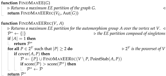 |
As expected, this algorithm is highly inefficient. As we will see in Section 5, it spends more than half an hour on the 4-hypercube graph with mere 16 vertices, 32 edges, and 384 automorphisms on an average desktop machine. Fortunately, as we will see shortly, this naïve algorithm can be greatly improved.
4.4. Building Larger EE Sets from Smaller Ones
In general, there is no need to consider all subsets of the current vertex set when searching for EE sets. Clearly, if P is not an EE set, neither is any of its supersets. However, we can go further: it turns out that a set is not worth consideration unless all of its subsets have been determined to be EE sets.
Lemma 2.
If a set is an EE set, all of its subsets are EE sets as well.
Proof.
Let A be an automorphism group, let P be an EE set with respect to A, and let be a subset of P. It holds that . Since the predicate ensures that there exists some automorphism for every permutation such that for every , the same must hold for every permutation . Therefore, holds, and is an EE set with respect to A. □
This observation suggests that the subsets of the current vertex set should be considered from smaller to larger. First, we find all 2-vertex EE sets. Having found all k-vertex EE sets, we proceed to -vertex subsets of the current vertex set, but we immediately discard a set unless all of the k-vertex sets , , …, have been found to be EE sets.
In practice, as we will see later, we find sets to be considered as potential larger EE sets by voting. A k-vertex set with casts a vote for each of the sets , …, . Following the voting procedure, only those -vertex sets that have garnered votes are checked to determine whether they are EE sets. Indeed, a set receives votes only if all of the sets , …, vote for it. This will only happen if each of these sets is a k-element EE set.
Note, however, that winning votes is only a necessary, but not sufficient, condition for a set to be an EE set. A counterexample is provided by the graph . Here, , , and are all 2-element EE sets, so they all cast a vote for the set . This set therefore receives three votes, but it is not an EE set.
4.5. Enforcing the Lower Bound for Score During Search
Lemma 3.
The score of an EE partition of a graph G cannot be greater than |Aut(G)|.
Proof.
By Theorem 1, the number of automorphisms of G (i.e., ) is divisible by the score of any EE partition of G. Therefore, the score cannot be greater than . □
Lemma 4.
Let , … be mutually disjoint subsets of V. If , …, are (some of the) equivalence classes of an EE partition , the score of cannot be greater than PointStab .
Proof.
Let us assume that we are building an EE partition with respect to some group A. We shall observe the following: if we are building an EE partition and have found the EE sets , the search for further EE sets is an independent subproblem, itself a search for an EE partition of the set with respect to the automorphism group . For any EE partition that we find as a solution to this subproblem, it must hold that because of Lemma 3. Therefore, the inequality must hold. □
Lemma 4 is immediately useful in the process of finding a maximum EE partition, since the score of an already constructed EE partition (or even the score of a partial EE partition; i.e., an EE partition ‘under construction’) can be used as a lower bound for the maximum attainable score. Furthermore, once all EE sets on the current level of recursion have been found, they should be considered from the largest to the smallest, in order to set the lower bound as high as possible as early as possible.
4.6. Exploiting Symmetry in Finding EE Sets and EE Partitions
Exploratory equivalence enables us to exploit symmetry (or, to take a look from a different angle, to reduce its adverse effects) in a pattern graph when searching for its occurrences in a host graph. However, it turns out that symmetry can also be put to use when searching for exploratory equivalence itself.
Lemma 5.
If is an EE set, then each of the members of Orbit is an EE set. If is not an EE set, then none of the members of Orbit is an EE set.
Proof.
Assume that is an EE set with respect to the automorphism group A, which implies . For every , there exists a such that . Furthermore, since holds, there exists an for every permutation p of P such that for every . However, since we can define a distinct permutation of in A for each such h as , must hold as well.
Let us now assume that P is not an EE set, but is. Then is also true and, as we have shown above, this implies that P is an EE set, which is a contradiction. □
In fact, EE sets themselves form equivalence classes, with two sets belonging to the same class if and only if they belong to the same orbit. Therefore, the right-hand column of Table 2 actually shows the equivalence classes of the EE sets of .
The notion of equivalence of EE sets can be naturally extended to EE partitions. For each EE partition, we can construct a set of equivalent EE partitions by applying the same composition of generators to each constituent equivalence class; for example, is an EE partition of , but so are and . Let us state this fact more formally:
Lemma 6.
Let , …, be the generators of an automorphism group A, and let with and , …, be the composition of an arbitrary sequence of generators. If is an EE partition, then so is .
Proof.
Let . Now, let us consider the set . We observe that it must stabilize the sets since, for every and , we have . We can also see that it must cover if covers , because for any permutation of , there exists a distinct permutation of . As we can see, the two conditions required for an EE partition must hold for if they hold for . □
Lemma 7.
Let be the set of all ordered EE partitions that start with an EE set P. For each EE set Orbit , we have . Furthermore, for each ordered EE partition in , there is an ordered partition in such that and the equivalence classes of have the same sizes as those of .
Proof.
This result follows from Lemma 6 since, for every and with , there exists a , where is the EE partition that we obtain from by applying g to all of its classes. Furthermore, the equivalence classes of have the same sizes as those of , and . Since is true as well, this also holds in the other direction. We thus have a bijection between and , so . □
Lemmas 5 and 7 effectively imply that we can restrict our attention to ‘representatives’ of the equivalence classes of EE sets, and any EE set in an equivalence class can be chosen as a representative. When building an EE partition, once we determine that P is an EE set, we can neglect all other members of , since we know that choosing P as the next equivalence class of the candidate EE partition being constructed will have the same effect as choosing any other member of for that role: the resulting candidate EE partition will have the same score as .
Recall that it makes no sense to check whether a k-element (with ) set P is an EE set unless we have determined that all of its -element subsets are EE sets. For instance, we proceed to checking whether is an EE set of only after we have discovered that the sets , , and are EE sets. These three sets, as evidenced by Table 2, belong to the same orbit. As it turns out, this is no coincidence:
Lemma 8.
If P is an EE set with elements, then all of its -element subsets belong to the same orbit.
Proof.
Let us assume that P is an EE set with respect to some automorphism group A. Let Q and R be subsets of P such that . By Lemma 2, the sets Q and R are also EE sets. Since holds, we have . One of the permutations within (say, g) has the property that , and hence . Since Q and R have been freely chosen, this holds for all subsets of P with size . □
This lemma provides a further boost to our algorithm. Imagine that we have discovered that is an EE set and would like to determine which of its supersets for are also EE sets. Without Lemma 8, we would have to consider all k-element subsets of in the voting procedure. However, Lemma 8 tells us that we only have to consider those k-element subsets of that belong to .
4.7. Two Further Improvements
We have seen that, during the search for candidate EE sets, we can downsize the number of the invocations of the costly function by proceeding from smaller to larger sets and by taking advantage of symmetry. However, we can reduce this number even further by observing that some EE sets may be extracted directly from the generators of the automorphism group. For example, one of the two generators of —namely, (123456)—represents an automorphism where vertex 1 is mapped to vertex 2, vertex 2 to vertex 3, …, and vertex 6 to vertex 1. By taking g to the 3rd power, we obtain the automorphism , where vertex 1 is mapped to vertex 4 and vice versa, and likewise for the pairs (2, 5) and (3, 6). Consequently, we can immediately infer that , , and are EE pairs of . This observation can be generalized to arbitrary permutation cycles of even length:
Lemma 9.
Let us assume that the generators of the automorphism group are represented as products of cycles. For each even-length cycle in those products, the sets , , …, are EE sets.
Proof.
Let be one of the cycles in the product-of-cycles representation of some generator g. Every generator is an automorphism, and so are their compositions. The automorphism g maps the vertices , , …, , to , , …, , , respectively, whereas the automorphism maps to (for all ) and to (for all ). Consequently, for each , the set is an EE set. □
The last improvement of the approach is purely technical: in some cases, the orbit of the same EE set P with respect to the same automorphism group would have to be computed twice: (1) when building a set of representative EE sets and (2) when searching for larger EE sets based on smaller ones. For this reason, we maintain a dictionary that maps a given EE set to its orbit with respect to the current automorphism group.
4.8. The Algorithm in Pseudocode
We are now ready to present the improved algorithm for finding a maximum EE partition. The pseudocode of the algorithm is shown in Algorithms 2–5. To provide a clearer overall picture of the algorithm, Figure 2 displays its simplified call graph, where a directed edge between two nodes indicates that the function corresponding to the source node invokes the function corresponding to the target node. The bottom part of each node presents a sample invocation of the corresponding function on a subgroup of the automorphism group of or an EE set of that graph. For example, the function FindEEPairs, if invoked on the automorphism group of , returns a set consisting of EE pairs , , and , which can be easily verified to be a representative set of EE pairs. (An equivalent output would be , , , since and .)
| Algorithm 2 Finding a maximum EE partition (part 1/4) |
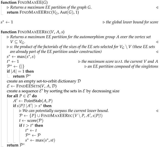 |
Figure 2.
A simplified call graph of the pseudocode presented in Algorithms 2–5.
Let us now turn our attention to individual functions. The function FindMaxEE, which serves as the entry point of the algorithm, and the recursive function FindMaxEERec, which is immediately invoked by FindMaxEE, are shown as Algorithm 2. The function FindMaxEERec is broadly similar to its namesake in the baseline algorithm (Algorithm 1). However, it calls a designated function FindEESets for producing a set of representative EE sets, rather than checking every subset of V to see whether it is exploratory equivalent. Another difference is that the new version maintains and uses the global lower bound for the maximum score (), which can be used to discard partial EE partitions that have no chance of exceeding the current maximum. To attain a high value early in the process, we consider the discovered representative EE sets from the largest to the smallest.
| Algorithm 3 Finding a maximum EE partition (part 2/4) |
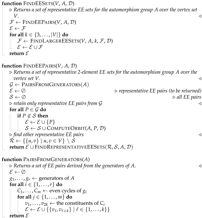 |
The function FindEESets (Algorithm 3) produces a set of representative EE sets for the given automorphism group over the given subset of the vertex set. Recall that only one EE set (although an arbitrary one) from each orbit can be declared the representative set of the orbit. The function starts with representative 2-element EE sets (called ‘EE pairs’ for simplicity) and then iteratively proceeds to larger sets. In the i-th iteration of the loop, the function discovers all representative ()-element EE sets from the pool consisting of representative ()-element EE sets.
The function FindEEPairs finds all representative EE pairs. By invoking the function PairsFromGenerators, it starts with the EE pairs that can be directly derived from the generators of the automorphism group. The function then finds out which of those EE pairs are representative; if two of them belong to the same orbit, at most one can be picked as the representative for that orbit. To find representative EE pairs that cannot be obtained directly from the generators, the function FindEEPairs calls the function FindRepresentativeEESets.
| Algorithm 4 Finding a maximum EE partition (part 3/4) |
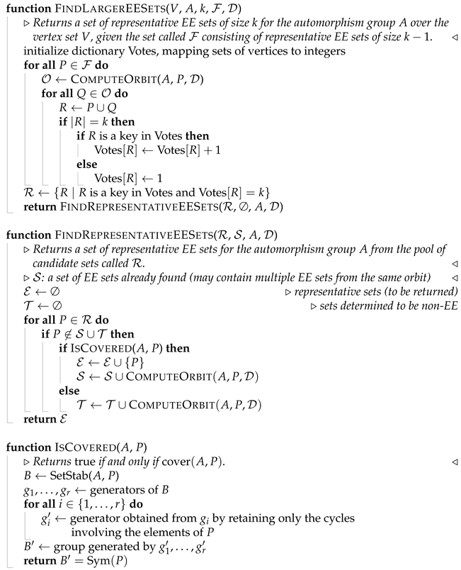 |
| Algorithm 5 Finding a maximum EE partition (part 4/4) |
 |
The function FindRepresentativeEESets (Algorithm 4) maintains a set of the subsets of V that have already been determined to be EE sets and a set of the subsets of V that have been proven to be non-EE sets. For each set P that belongs neither to nor to , the function checks to see whether it is covered by the set of automorphisms. If it is, the entire orbit of the set P is added to the set ; otherwise, the orbit is added to the set . An EE set is added to the output set only if none of the sets in its orbit have been added to . Thereby, we ensure that exactly one EE set from each orbit is added to the set of representative EE sets.
The function FindLargerEESets (Algorithm 4) accepts a set of representative EE sets of size and returns a set of representative EE sets of size k. It relies on the fact that a necessary condition for a set to be an EE set is that all of its ()-element subsets are EE sets themselves (Lemma 2) and that, moreover, all of those ()-element subsets belong to the same orbit (Lemma 8). To find the potential k-element EE sets, we proceed as follows. Starting with a ()-element EE set P, we search its orbit for all sets Q that can be obtained from P by removing one vertex in P and adding one vertex not in P. The two ()-element sets P and Q are both subsets of the same k-element set , and so both P and Q cast a vote for R. If, after the entire orbit of P has been scanned, the set R has gathered k votes, we know that all of its subsets are EE sets. Consequently, R is considered a potential EE set and is placed into a pool . At the end, just like the function FindEEPairs, the function FindLargerEESets calls the function FindRepresentativeEESets to find those sets in the pool that are exploratory equivalent and to make sure that only one EE set remains from each orbit.
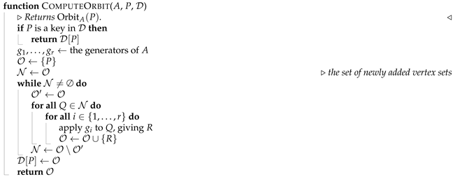
Finally, the function ComputeOrbit (Algorithm 5) computes the orbit of a given EE set with respect to the given automorphism group. The function simply maintains a set of vertex sets that have already been determined to belong to the orbit of the input set. In each iteration, the function applies each generator to all vertex sets that have been added to in the previous iteration (at the beginning, this is just the input vertex set) and adds the resulting vertex sets to the set . The loop is finished once it turns out that nothing more can be added to . The ensuing set is the orbit of the input EE set, and it is added to the dictionary to avoid its potential repeated computation.
4.9. Correctness
Theorem 2.
For a given graph, the function FindMaxEE in Algorithm 2 reports a maximum EE partition.
Proof.
An ordered EE partition is a sequence of EE sets. Clearly, if we consider every possible EE set for each position in the sequence, we will have considered all EE partitions by the end of the search process. By keeping track of the maximum-score EE partition constructed so far, we will ultimately arrive at a maximum EE partition.
However, by Lemma 7, we need not consider every EE set at every step (i.e., in every recursive invocation of the function FindMaxEERec), but only one EE set per orbit. As we will show later, the function FindEESets does just that. Furthermore, by Lemma 4, we can safely discard an EE partition being constructed if its maximum potential score falls short of the maximum product of the factorials of the class sizes encountered so far (the value in Algorithm 2). It is easy to see that the function FindMaxEERec updates and uses the value in such a way that at least one maximum EE partition remains.
The function FindEEPairs finds all representative 2-element EE sets for the given automorphism group. Following the code that extracts representative EE pairs directly from the generators, the basis of which is provided by Lemma 9, the function FindEEPairs calls FindRepresentativeEESets to discover representative EE pairs from the pool of remaining vertex pairs. In FindRepresentativeEESets, each pair that has been determined to be an EE set is added to the output set, provided that it is not yet a member of the set , which is the union of the orbits of the EE pairs found so far. In this way, we ensure that all EE pairs are considered but only representatives of the individual orbits are actually returned from the function.
The function FindLargerEESets first builds a pool of potential k-element EE sets given the set of representative -element EE sets using a straightforward voting scheme and the conditions established by Lemmas 2 and 8. Following that, it extracts from the pool a set of representative k-element EE sets in much the same way as the function FindEEPairs (both functions call FindRepresentativeEESets to this end). The function FindLargerEESets thus finds all representative k-element EE sets, provided that it has been given all representative -element EE sets.
We have seen that the function FindEEPairs finds all representative EE pairs, while the function FindLargerEESets finds all representative k-element EE sets from representative -element EE sets. Therefore, the function FindEESets returns all representative EE sets for the given automorphism group. Considering the discussion from the first two paragraphs of this proof, we can conclude that the function FindMaxEE finds a maximum EE partition. □
4.10. Implementation
The algorithm has been implemented in the Python programming language (version 3.10.12) coupled with the Sage framework (version 9.5; https://www.sagemath.org). To compute the pointwise stabilizer and the setwise stabilizer of an automorphism group with respect to a vertex set, we invoke the corresponding built-in Sage function. We would do the same to compute the orbit of a given vertex set were it not for the surprising fact that our own Python implementation, which follows the function ComputeOrbit in Algorithm 5, actually performs faster.
The full Python–Sage implementation is accessible at https://github.com/firsht1/ee, accessed on 21 September 2026.
4.11. Computational Complexity
Our objective was not to improve the theoretical computational complexity but to devise a viable algorithm that would perform reasonably well on a majority of symmetry-rich graphs of reasonable sizes. Nevertheless, a brief discussion on this topic will not hurt.
We will not attempt to derive a formula for computational complexity, since this is not the purpose of this paper, but it might still be useful to identify the main factors that contribute to the overall complexity:
- (1)
- The size of the largest EE set.
- (2)
- The cost of computing the cover predicate.
- (3)
- The cost of computing the orbit.
- (4)
- The cost of potential backtracking in the recursive FindMaxEERec function.
Let us first focus on factor (1). To find an EE set of size s, the algorithm has to enumerate all subsets of sizes 2, …, , for a total of subsets. If , we arrive at a factor of .
Regarding factors (2) and (3), recall that computing the cover predicate takes exponential time, while the orbit can be found in polynomial time [23]. It is therefore important to compute the cover predicate for as few sets as possible.
The fourth factor is hard to estimate, but by considering the candidate EE sets on each level of recursion from the largest to the smallest and by maintaining the lower bound for maximum EE score, we can hope to reduce backtracking as much as possible.
Since exploratory equivalence is closely connected to the automorphism group, an interesting question is how the size of that group (i.e., the number of automorphisms) affects the computational complexity. Surprisingly, there appears to be no direct link between these two measures; the number of automorphisms affects the running time only indirectly, through the factors given above. In particular, a larger number of automorphisms may lead to a larger number of EE sets, potentially causing a greater amount of backtracking and also influencing factors (2) and (3). Alternatively, a larger automorphism group may lead to larger EE classes and thus affect factor (1). Therefore, the effect of the number of automorphisms on the computational complexity of the improved algorithm is adequately captured by the factors (1) through (4) listed above.
As we have seen, even the improved algorithm may take exponential time with respect to the input size in the worst case. This should not surprise us, for we proved that finding a maximum EE partition is NP-hard [8]. If we actually managed to bring the worst-case time complexity down to polynomial, this would imply a major collapse of the computational complexity hierarchy or, much more likely, a serious error in our thought process.
To conclude this section, we will try to estimate the computational complexity of the improved algorithm for two specific graph families: complete graphs () and path graphs (). The graph has n vertices and an edge between each distinct pair of vertices, while the graph has n vertices and an edge between vertices i and , for all .
The graph has the maximum possible number of automorphisms (), and its sole maximum EE partition is simply . If run on , the proposed algorithm for finding a maximum EE partition will start with a single 2-element set (say, ), discover that it is an EE set, and compute its orbit, which contains all 2-element subsets of the vertex set V. Following that, it will start the voting procedure and find out that each of the 3-element subsets of V has received three votes. By checking one of those sets to see if it is an EE set and computing its orbit, it will have determined that all 3-element subsets of V are EE sets. The algorithm will then proceed to 4-element subsets, etc., effectively enumerating all subsets of V in the process. This directly gives a complexity of , but we may be confident that it is actually , since (1) there is absolutely no backtracking (once the algorithm discovers the EE set , it has effectively finished); (2) the costly setwise stabilizer is computed only for of those sets (for a single 2-element set, for a single 3-element set, etc.).
The case is quite different. For all , the graph has only two automorphisms, and one of its maximum EE partitions is . Naturally, only has EE sets of size 2: these are , for . Unfortunately, these sets do not belong to the same orbit; instead, each forms its own orbit, while the 2-element non-EE sets (these also have to be considered, since the algorithm does not ‘know’ in advance which set is an EE set) form orbits of size 2 at most. This means that the algorithm will have to compute the cover predicate for subsets of V, giving a complexity that is exponentially dependent on . However, backtracking poses no problems, since choosing any 2-element EE set as the first equivalence class will set the lower bound to and effectively eliminate the alternatives.
5. Experimental Results and Discussion
Having presented the improved algorithm for finding a maximum exploratory equivalent partition, we proceed to its experimental validation. To provide a better insight into the effect of individual improvements, we also run the tests using an implementation of the baseline algorithm (given as Algorithm 1) and three ‘intermediate’ versions, each building upon the preceding version by including one more improvement.
This section is structured as follows. In Section 5.1, we describe the graph sets on which we tested the five programs. In Section 5.2, we present the experimental setup in detail. Section 5.3, Section 5.4, Section 5.5, Section 5.6, Section 5.7 and Section 5.8 present and discuss the results of the experiments. Following that, we briefly discuss the ordering sensitivity exhibited in some cases (Section 5.9). In Section 5.10, we focus on memory consumption (all experiments in the preceding sections feature only time measurements). Section 5.11 provides a short summary of the findings.
All our experiments were carried out on a Linux desktop machine (Lenovo Group Ltd., Morrisville, NC, USA) with the Intel Core i7-7700 processor (Intel Corp., Santa Clara, CA, USA) and 32 GiB of RAM. For each experiment, we measured the total wall-clock time of computing a maximum EE partition for the corresponding graph using the corresponding program.
5.1. Test Graph Sets
We tested our algorithms on the six following graph families:
- Cycle graphs. The k-cycle graph (; ) is composed of k vertices and k edges. (We chose k to denote the parameter of the family (instead of the more usual n) to avoid the confusion between the parameter and the number of vertices (n), which may, in general, be different from k.) The edges are and for . The number of automorphisms of is .
- Complete graphs. The k-complete graph (; ) is composed of k vertices and edges, since there is an edge between each pair of vertices. The number of automorphisms of is .
- Hypercube graphs. The k-hypercube graph (; ) is made up of vertices, which are customarily identified by k-bit vectors, and an edge whenever the Hamming distance between the bit vectors representing u and v is exactly 1. The graph has edges and automorphisms.
- Square-grid graphs. The k-square-grid graph (; ) consists of vertices denoted by (for and ) and an edge between and whenever either and or and . Every graph from this family has exactly 8 automorphisms.
- Cross-polytope graphs. The graph () has vertices, denoted 1, …, , and edges. Vertices u and v are connected if and only if . The graph has automorphisms.
- GI-graphs. These highly symmetrical graphs [25] are parameterized by an integer and a multiset such that and for . The graph (or ) comprises vertices (denoted for and ) and
- an edge between and for all distinct and all ;
- an edge between and for all and all , where + is performed modulo k;
- an edge between and for all and all , where − is performed modulo k.
For the sake of conciseness, we will not reproduce the formula to compute the number of automorphisms here and instead refer the interested reader to the original paper [25].
In contrast with the remaining graph sets, which are parameterized by a single integer, there are multiple ways to build a meaningful family of GI-graphs. We decided to fix and restrict the elements of the multiset J to belong to the set , with additional stipulations that at least two elements of J be distinct, that , and that the number of automorphisms not exceed , the upper bound for Sage’s integral data type. The graphs in the family were ordered primarily by the increasing , starting with , and secondarily by the increasing number of automorphisms.
The reason for choosing these graph families is twofold. First, all families except for the GI-graphs are parameterized by a single parameter, which is directly associated with the size of the graph. Second, to determine the merit of the improved algorithm, we have to test it on graphs with a sizable number of automorphisms, since these are likely to have large maximum EE scores. Complete graphs, hypercube graphs, and cross-polytope graphs are well known to be highly symmetric, while the less-known GI-graph family was—according to its inventors [25]—specifically designed to be rich in the number of automorphisms. Cycle graphs and square-grid graphs are somewhat different in this regard but, as we will see later, both families serve to illustrate some interesting aspects of the algorithm.
Table 3, Table 4, Table 5, Table 6, Table 7 and Table 8 give the properties of selected graphs from our test sets. For each family, we picked the first five members and the last five members on which we tested the improved algorithm. The columns in each table represent the parameter value (k or J), the number of vertices, the number of edges, the size of the automorphism group, and the score of a maximum EE partition given as the product of the factorials of the sizes of its classes, respectively. To save space, the multiset J is represented as the concatenation of its elements (for example, 223 stands for ).
Table 3.
The cycle graph family.
Table 4.
The complete graph family.
Table 5.
The hypercube graph family.
Table 6.
The square-grid graph family.
Table 7.
The cross-polytope graph family.
Table 8.
The GI-graph family.
Figure 3 and Figure 4 depict a handful of graphs from each test family. An exception is the GI family; instead of the graphs and , the first and the fourth members of the family, we show the graphs and , which are structurally similar but small enough to fit the width of a page.
Figure 3.
Selected members of the cycle graph family, complete graph family, hypercube graph family, and square-grid graph family.
Figure 4.
Selected members of the cross-polytope graph family and two sample GI-graphs.
5.2. Experimental Design
We performed 30 series of experiments, in which each of the five programs (Python–Sage implementations of the respective algorithms) was tested on each of the six graph families. The programs were defined as follows:
- Version 1 (the baseline program). The implementation of the baseline algorithm closely followed the pseudocode given in Algorithm 1.
- Version 2. For this version, we extended the baseline program with the improvement described in Section 4.4. In particular, for , we did not test a k-element subset of the current vertex set for being an EE set until we established that all its subsets are EE sets. Having found all k-element EE sets, we discovered potential -element EE sets by voting.
- Version 3. To obtain the third program, we extended version 2 with the logic introduced in Section 4.5. Specifically, the construction of a candidate EE partition is cut short if we find out that its maximum attainable score cannot be greater than the score of the maximum complete or partial EE partition discovered so far.
- Version 4. Here, we used the findings presented in Section 4.6 to further enhance version 3. This means that we took advantage of the fact that EE sets themselves form equivalence classes in order to reduce the number of EE sets that have to be considered.
- Version 5 (the final program). By including the improvements explained in Section 4.7 (a rule to obtain a set of initial EE pairs directly from the generators of the current automorphism group and maintaining an EE-set-to-orbit dictionary on each level of recursion), we arrive at an implementation of the final algorithm; i.e., the one that is shown in Algorithms 2–5 in this paper.
Every version thus includes everything from its predecessor, together with an extra improvement. To ease the presentation, we use the wording ‘improvement ’ to refer to the difference between version i and its successor. For instance, improvement refers to the improvement presented in Section 4.6, which distinguishes version 3 from version 4.
For each pair of a program and a graph family, we ran the program on the graphs in that family in the order of increasing parameter until we encountered the first graph that required more than one hour. Additionally, we stopped the series once the parameter k exceeded 100 (for all families except GI, where k was fixed at 30).
5.3. Results on the Cycle Graph Family
We present and discuss the results for each family separately. In this section, we focus on cycle graphs. Table 9 shows how the time consumption for each of the five programs depends on the growing parameter k (which, in this case, is equal to n, the number of vertices).
Table 9.
Time consumption (in seconds) for cycle graphs ().
The baseline program tests the cover predicate for each subset of , so its time consumption clearly grows exponentially with the parameter k. This is true for every graph family.
Cycle graphs appear to be the easiest case for our experimental setup, since the number of edges and automorphisms grows linearly with the number of vertices. Indeed, even the baseline program managed to arrive to before hitting the 1-h time limit, and the final program did not reach this boundary until approximately . However, what is interesting is the seemingly anomalous growth of time consumption with respect to the parameter k for some versions; often, a larger graph required less time than a smaller one. This behavior, however, can be readily explained by the variation in the structure of maximum EE partitions with increasing k. As we showed in [9], the structure of the maximum EE partition depends on the divisibility of k with 2 and 3:
- If (i.e., if k is divisible by 3), a maximum EE partition consists of a single 3-element class, which is made up of three equally spaced vertices. (Needless to say, the rest of the EE partition consists of the singletons capturing the remaining vertices.)
- If (i.e., if k is even and not divisible by 3), a maximum EE partition consists of two 2-element classes; one of them comprises two antipodal vertices, and the other is formed by the two neighbors of one of the vertices from the first class.
- If (i.e., if k is odd and not divisible by 3), a maximum EE partition consists of a single 2-element class, an arbitrary 2-element subset of V.
Figure 5 shows the growth of time consumption with respect to k for the combination of version 5 and all three subsets of . We can see that the cases and are more favorable than the case . If k is odd and not divisible by 3, the maximum EE partition comprises a single 2-element class, and once the algorithm discovers this class (any 2-element subset of V will do) and stabilizes the automorphism group with respect to it, the residual automorphism group only consists of the identity automorphism. On the first level of recursion in the function FindMaxEERec (Algorithm 2), the algorithm still tries a couple of other 2-element subsets of V to fill the role of the first class in the nascent EE partition, since not all 2-element subsets of V belong to the same orbit (for example, Table 2 lists the orbits of ). However, none of these alternatives can surpass the maximum score attained by the first choice.
Figure 5.
The consumption of time as a function of k when running version 5 on cycle graphs.
The case is similar. Once the algorithm discovers a three-element EE set and stabilizes the automorphism group with respect to it, the residual automorphism group consists of a single automorphism. Again, the alternatives on the first-level of recursion cannot compete with the selection of the three-element EE set (which is tried first, since on each level of recursion, the algorithm considers the EE sets in the decreasing order of their size). This holds true even if k is divisible by 6. The alternative high-score EE partitions (those consisting of two 2-element classes) are discouraged, since .
The case gives the algorithm more work. In contrast to the other two cases, the algorithm is not yet ‘almost done’ once it discovers the first EE set, since the residual automorphism group still covers a two-element set. Considering the aforementioned fact that not all 2-element vertex sets belong to the same orbit, the algorithm will have to consider multiple alternatives on two levels of recursion, rather than just one.
Focusing on individual versions, improvement vastly boosts performance, since it tests a larger candidate EE set for satisfying the cover predicate only after having determined that all of its subsets are exploratory equivalent. Since no cycle has an EE set larger than 3, version 2 never considers vertex sets of sizes 4, 5, etc., while the baseline algorithm does. Improvement speeds up the performance on even cycles, regardless of whether k is (also) divisible by 3; in this case, many EE partitions are composed of two classes, which means that enforcing a lower score bound during search will definitely help. Improvement provides a further boost, since most EE pairs have an orbit of size k (for example, the orbit of the EE pair {1, 2} consists of all pairs of adjacent vertices), and so the number of representative EE pairs will be significantly smaller than the total number of EE pairs. Improvement helps only marginally; as we shall see later, it is more beneficial in the presence of larger EE classes.
5.4. Complete Graphs
The maximum EE partition of the graph is simply . Its score, , is equal to the number of automorphisms.
Table 10 shows the results for the family of complete graphs (again, k is the same as n, the number of vertices). As with cycle graphs, the baseline program tests the cover predicate for each subset of , so its time consumption can only grow exponentially with respect to k. Improvement has virtually no effect, since all subsets of are EE sets; it does not matter whether we generate them from smaller to larger via voting or in some other manner. Improvement has a more significant impact: setting a lower bound for the maximum EE score does eliminate some competitive (but inferior or equivalent) EE partitions. Even greater savings are provided by improvement , the reason for which is clear: for each EE set of size s, its orbit consists of all sets of s vertices. Consequently, for each s from 1 to k, we essentially work with a single EE set rather than EE sets. However, in the voting procedure, we still have to enumerate all EE sets in order to find the EE set(s) of size , which is why we cannot escape exponential growth of time. Improvement also brings some benefits: the computation of the orbit of a (large) EE class may be costly, and so the set-to-orbit dictionary indeed saves some time.
Table 10.
Time consumption (in seconds) for complete graphs ().
5.5. Hypercube Graphs
A maximum EE partition of is . For all other , one of the EE partitions of is a partition composed of two classes—one consisting of two antipodal vertices (say, and ), and the other consisting of the neighbors of one of these two vertices (say, , , , …, , and ). It is strongly suspected (although not yet proven) that is actually a maximum EE partition of .
As shown in Table 11, hypercube graphs are highly conducive to the improvements of the baseline algorithm. In particular, the largest graph successfully completed within the 1-h time limit by the baseline program and version 2 is (16 vertices, 32 edges, 384 automorphisms), although version 2 spends only a hundredth of the time on it compared with version 1. Version 3 manages to process (64 vertices, 192 edges, 46,080 automorphisms), whereas versions 4 and 5 reach as far as (1024 vertices, 5120 edges, ≈3.7 × automorphisms).
Table 11.
Time consumption (in seconds) for hypercube graphs ().
Improvement is almost always beneficial; a rare exception is the complete graph family, where every subset of is an EE set. Improvement helps primarily because of the presence of large EE classes ( has an EE partition with a class of size k). Since the algorithm is designed to find large EE sets early in the process, it quickly sets the lower bound for the maximum EE score to , ruling out many candidate (partial) EE partitions.
Improvement helps because hypercube graphs have relatively few distinct orbits of EE sets, which are therefore fairly large on average. For example, the graph has 496 two-element EE sets and 320 three-element EE sets, but only six distinct orbits of 2-element EE sets and a single orbit of 3-element EE sets. As a consequence, when the algorithm discovers an EE set of size 3, it will discover all the remaining 319 three-element EE sets just by computing the orbit of that set, without having to determine which of those 319 sets are covered by the current automorphism group and which are not.
The last improvement also makes itself felt. As with complete graphs, the reason for this result is the presence of large EE classes. If we avoid recomputing their orbits, we will certainly save some time.
5.6. Square-Grid Graphs
For the preceding two families (complete graphs and hypercube graphs), the size of the largest EE class is (almost) the same as the parameter k, so even with all the improvements, the time consumption grows exponentially with k. However, even if the size of the largest class is constant, we may still arrive at an exponential complexity. As we saw in Section 4.11, one such case is given by path graphs. Square-grid graphs represent another example. As evidenced in Table 12, the time increases exponentially with k even though for all , a maximum EE partition is composed of two classes of size 2, and no EE partition has a class of size 3. The reason is that square-grid graphs have a large number of small orbits of EE pairs, making it necessary to compute the costly cover predicate for a vast majority of EE pairs.
Table 12.
Time consumption (in seconds) for square-grid graphs ().
To be more concrete, there are unordered pairs (2-element sets) of vertices for the k-by-k grid. However, the size of the orbit of a pair may be 2, 4, or 8, regardless of k (Figure 6). As a consequence, the costly cover predicate has to be computed for more than pairs. Considering the fact that computing the cover predicate takes exponential time, we should not wonder that the time consumption as a whole grows exponentially with k.
Figure 6.
The graph . The size of the orbit is 2 for the EE pairs along either diagonal (such as (0, 15) and (6, 9)), 4 for all other EE pairs (such as (0, 3), (0, 12), (0, 15), (1, 2), (1, 4), (1, 11), (1, 13), and (1, 14)) and for non-EE pairs along either diagonal (such as (0, 10) and (6, 12)), and 8 for all other pairs.
5.7. Cross-Polytope Graphs
One of the EE partitions of the graph with vertices 1, 2, …, is . Another is . To see that these partitions are indeed exploratory equivalent, it is helpful to consider the complement of , which is composed of k distinct 2-vertex path graphs. (The complement of a graph , i.e., the graph with , has exactly the same automorphism group as the graph G and, hence, also the same EE partitions.) Since for all , is a maximum EE partition for , whereas for and , attains a greater score.
Considering that a maximum EE partition is composed of a single large EE class for all but the smallest values of k, the performance of the algorithms on cross-polytope graphs is expected to exhibit a behavior similar to what we have seen on complete graphs. By inspecting Table 13, we can confirm that this is indeed the case.
Table 13.
Time consumption (in seconds) for cross-polytope graphs ().
5.8. GI-Graphs
For this family, it is harder to draw definite conclusions, as both the number of automorphisms and the maximum EE score may vary widely between successive members of the family. However, every maximum EE partition in the test set consists of at least one class of size three or more, and many partitions contain even larger classes. For this reason, it is expected that all improvements, except perhaps the last, make themselves felt. As shown in Table 14, our expectations have been met as far as improvements , , and are concerned. However, improvement sometimes unexpectedly increases the time consumption. The reason is that when finding EE pairs, version 5 starts with the pairs that can be obtained directly from the generators, although it ultimately produces the same set of EE pairs as version 4, only their order in the list differs. However, a different order of EE pairs may result in a different order of discovering candidate EE partitions, which, in turn, may lead to a faster or a slower progress towards a maximum EE partition. A brief discussion on ordering sensitivity is provided in Section 5.9.
Table 14.
Time consumption (in seconds) for GI-graphs ().
The GI-graphs provide a good example for the observation that the sheer number of automorphisms (and, in turn, the closely related maximum EE score) does not directly affect the time consumption. Figure 7 shows a plot of time consumption versus the number of automorphisms for the graphs with (note that the scale on the x axis is logarithmic) and version 5. While we may observe a generally upward trend, it is adequately explained by the size of the maximum EE class (which directly affects the computational complexity) and the number of EE classes (which has an indirect effect, through a potentially greater amount of backtracking).
Figure 7.
The consumption of time as a function of the number of automorphisms when running version 5 on GI-graphs with and .
5.9. Ordering Sensitivity
As we noted in Section 5.8, version 5 in some (rare) cases performed more slowly than version 4. This apparent anomaly is not directly associated with improvement ; rather, it stems from the fact that it is important how the EE sets considered in the for-loop of the function FindMaxEERec (Algorithm 2) are ordered. We already know that they have to be ordered from the largest to the smallest, so as to set a high global lower bound ( in Algorithm 2) for the maximum EE score early in the process, but sometimes even the order of EE sets of the same size matters.
To provide an example, let us focus on the graph in Figure 8. This graph has several 2-element EE sets, but no 3-element EE set. If the algorithm picks the EE set {1, 2} on the first level of recursion, it will select either the EE set {3, 4} or the set {5, 6} on the second level. In either case, the bound will be set to , preventing all of the alternative EE sets from being chosen in the subsequent iterations of the for-loop back on the first level of recursion. However, if is chosen on the first level, the algorithm will not find any EE set on the second level, and the bound will be set only to . Consequently, the algorithm will still have to consider the alternative EE sets on the first level.
Figure 8.
A graph to illustrate ordering sensitivity.
5.10. Memory Consumption
In the previous sections, we focused exclusively on time consumption. Now, we are interested in the peak amount of memory allocated by our implementations, which we measured using Python’s standard tracemalloc utility. This utility only measures the amount of memory occupied by Python objects (such as lists, tuples, sets, and dictionaries), whereas objects created within the Sage framework (such as graphs or permutation groups) are not tracked. Fortunately, this is not really an issue, since most of the data that we actually work with and that actually tangibly scale with the growing parameter k are represented as usual Python objects. For example, a set of EE sets is represented as a Python set (or list) of Python tuples, not as a Sage object opaque to the Python interpreter. Graphs and permutation groups are stored as Sage objects, but these may be regarded as the input data. Furthermore, recall that a permutation group is stored efficiently, as a set of generators rather than a full set of automorphisms.
Table 15 shows the peak amount of memory allocated by version 5 for each graph family except the GI-graphs. A major memory consumer is the voting process in the FindLargerEESets function. For example, in the case of the complete graphs, the orbit of an m-element EE set consists of all m-element subsets of the vertex set, and each of those sets casts a vote for all of its one-element extensions. All m-element sets and their votes are simultaneously kept in memory. Another non-negligible source of memory allocation is the set-to-orbit dictionary introduced in version 5 to prevent duplicate time-consuming orbit computations.
Table 15.
Peak memory allocation (in MiB) when running version 5 on each graph family.
Unsurprisingly, the peak amount of allocated memory grows with k in a manner similar to time consumption. For example, the complete graphs exhibit an exponential growth of memory consumption, which can be readily explained by the above-mentioned fact that all m-element subsets of the vertex set have to be kept in memory before proceeding to -element EE sets. By contrast, for the cycle graph family, the growth is much more gentle, but the ‘bumps’ are similar to those observed in the time consumption data (cf. the rightmost column of Table 16). In particular, the cases where the number of vertices is divisible by 2 but not by 3 are more demanding than the other cases, both temporally and spatially.
Table 16.
Peak memory allocation (in MiB) when running each version on the complete graphs family.
Table 16 shows how the peak memory consumption for the complete graphs family differs between the versions of the algorithm. Since all subsets of the vertex set are EE sets, there is no significant difference between versions 1 and 2. However, versions 3 and 4 both reduce the memory consumption: maintaining and imposing the lower bound for the maximum EE score and taking into account the equivalence of EE sets both reduce the number of EE sets that have to be simultaneously kept in memory. Version 5 introduces the set-to-orbit dictionary and thus again causes the memory consumption to increase.
5.11. Summary of the Results
For all graph families, there is a huge leap from the baseline algorithm (version 1) to the improved algorithm (version 5). However, the influence of the individual improvements varies from family to family. Improvement provides a large boost for all families except for complete graphs, where all subsets of V are exploratory equivalent and so it does not matter whether larger EE sets are simply generated or built in a bottom-up manner by voting. Improvement is evident for all graph families, but its effect is comparatively weak for cycles and square grids, where maximum EE partitions are made up of a small number (1 or 2) of small classes (of size 2 or 3). Improvement is once more a major contribution to the overall speed; it is weakest (but still considerable) in the case of square grids, where the orbit sizes are small and independent of k. Lastly, improvement does not have a profound impact, but is still noticeable in the presence of large EE classes. We can thus conclude that all improvements are meaningful and may recommend that the proposed improved algorithm be used for finding maximum exploratory equivalent partitions in graphs.
In Table 17, we provide yet another view on the benefits of individual improvements. For each version of the algorithm and for each of the four selected graph families, we give the largest graph that was processed by that version within an hour. (We decided to omit cycle graphs and GI-graphs, where we did not strictly adhere to the 1-h time limit.) We can observe a significant increase in all four quantities (the parameter k, the number of vertices, the number of edges, and the number of automorphisms) between the first and the last version, once again confirming the value of the proposed approach.
Table 17.
The largest graph processed within an hour.
6. Conclusions
In this paper, we presented an improved algorithm for finding a maximum exploratory equivalence in a graph. First, we observed that the classes that make up an EE partition can be discovered from smaller to larger by an efficient voting procedure. Following that, we found that maintaining the lower bound for the maximum EE score rules out many non-maximum EE partitions before they are actually built. Third, we exploited the symmetry in EE sets themselves to reduce the number of the subsets of the vertex set that have to be checked as potential candidates for EE sets.
As shown by the experiments, these improvements had a significant impact on performance. The improved algorithm was tested on multiple symmetry-rich graph families, and a notable reduction in time consumption was observed for each of them. Despite the fact that the worst-case complexity of the algorithm remains exponential (the underlying problem is NP-hard), we may claim that we have significantly improved the practicability of the problem of finding a maximum exploratory equivalent partition of a graph. To the best of our knowledge, the approach presented in this paper is the first improvement of the exact algorithm for finding a maximum EE partition.
We may now ask ourselves how much room for additional improvement we still have, save from rewriting the algorithm in a more efficient programming language such as C/C++, where we cannot expect more than a constant-factor boost. As we proved in our previous paper [8], we cannot possibly hope for a polynomial algorithm without causing a collapse in the computational complexity hierarchy. We have no proof, but we sincerely doubt that a significant further improvement can be brought about for graph families where the size of the largest EE set grows proportionally with the graph size (such as complete graphs and cross-polytope graphs). However, there are graph families, such as square grids, where the EE sets are small and even the size of the automorphism group grows slowly or remains constant with graph size, but the time to find a maximum EE partition still grows exponentially, since there are many instances of small but not directly related EE sets. For such cases, we might have to devise a stronger model of relationship between EE sets or more thoroughly exploit the information ‘hidden’ in the generators of the input graph’s automorphism group. Currently, only a relatively small proportion of EE sets are typically extracted directly from the generators, while all others are found by computing the orbit or the cover predicate. If we were able to extract more EE sets (or non-EE sets) without resorting to costly measures, the algorithm could be further improved.
Author Contributions
Conceptualization, L.S., U.Č., J.M. and L.F.; methodology, L.S., U.Č., J.M. and L.F.; software, L.F.; validation, L.S., U.Č., J.M. and L.F.; formal analysis, L.S., U.Č., J.M. and L.F.; investigation, L.S. and L.F.; data curation, L.S. and L.F.; writing—original draft preparation, L.S. and L.F.; writing—review and editing, L.S., U.Č., J.M. and L.F.; visualization, L.F. All authors have read and agreed to the published version of the manuscript.
Funding
This research was supported internally by the Faculty of Computer and Information Science, University of Ljubljana. No specific grant or project number applies.
Data Availability Statement
Both the code and the data used in the preparation of this manuscript are available in their entirety at https://github.com/firsht1/ee, accessed on 21 September 2026. The experiments presented herein may be fully replicated using the provided materials. Potential users are encouraged to consult the corresponding author, should they need any help.
Acknowledgments
We would like to thank the anonymous reviewers for their insightful comments. Additionally, we are grateful to the research team that invented the VF2 algorithm for their intuitive implementation, which could be effortlessly modified to include the code for enforcing the EE-derived constraints. They made the part of our work described in the Appendix A considerably easier than we expected it to be.
Conflicts of Interest
The authors declare no conflicts of interest.
Appendix A. Exploratory Equivalence and Subgraph Isomorphism
Although the relationship between exploratory equivalence and subgraph isomorphism is not the main focus of this paper, it is still of interest to determine whether—and to what extent—the constraints derived from a maximum EE partition speed up subgraph isomorphism search. To this end, we modified the source code of the VF2 algorithm [26] (available online: https://github.com/MiviaLab/vf2lib, accessed on 21 September 2026) to respect the EE-derived constraints during its search for monomorphisms between the pattern graph and the host graph. Recall that an EE partition with for gives rise to the constraints for . To enforce these constraints during the search for monomorphisms , we prevent a match between a vertex and a vertex if there exists a vertex such that and .
To assess the value of this approach, we carried out two series of experiments. In the first series, we searched for all occurrences of the graph (the 4-cycle graph) in the graph (the k-by-k square grid) for . In the second series, we searched for all occurrences of the graph (the complete graph on 4 vertices) in the graph , for . In both sets of experiments, we compared the time spent by the original VF2 algorithm with the time spent by the modified algorithm for each k. The results are shown in Table A1 and Table A2.
Table A1.
Time (in milliseconds) required by the original and the modified VF2 algorithm to find all occurrences of in .
Table A2.
Time (in milliseconds) required by the original and the modified VF2 algorithm to find all occurrences of in .
A maximum EE partition of is , giving the constraints and . The theoretical speedup for the first set of experiments (finding all occurrences of in ) is thus . While the modified VF2 algorithm does indeed find only a quarter of the -to- monomorphisms discovered by the original algorithm (without losing any actual occurrence of in ), the time consumption ratio is approximately 2 for sufficiently large host graphs. The reason for the disparity between the theoretical and practical speedup is that a superfluous monomorphism between and cannot be suppressed and discarded until it has at least partially been created. In particular, a superfluous monomorphism with will be suppressed only after pattern-graph vertices 1 and 2 have already been matched to the corresponding host-graph counterparts, whereas a monomorphism with and will only be discarded after vertices 1, 2, and 3 have been matched.
In the second series of experiments (finding in ), the actual time consumption ratio was much closer to a theoretical speedup of . The EE-derived constraint means that many superfluous monomorphisms will be suppressed at the moment when vertex 2 is about to be matched; if the algorithm finds out that , it will not develop the monomorphism h any further. By contrast, in the first series, we had to wait at least until vertex 3 to be able to discard a monomorphism.
References
- Deo, N. Graph Theory with Applications to Engineering and Computer Science; Dover Publications: Garden City, NY, USA, 2016. [Google Scholar]
- Easley, D.; Kleinberg, J. Networks, Crowds, and Markets: Reasoning about a Highly Connected World; Cambridge University Press: Cambridge, UK, 2010. [Google Scholar]
- Trinajstić, N. Chemical Graph Theory, 2nd ed.; CRC Press: Boca Raton, FL, USA, 2019. [Google Scholar]
- Toth, P.; Vigo, D. Vehicle Routing: Problems, Methods, and Applications; Society for Industrial and Applied Mathematics: Philadelphia, PA, USA, 2015. [Google Scholar]
- Han, M.; Kim, H.; Gu, G.; Park, K.; Han, W. Efficient Subgraph Matching: Harmonizing Dynamic Programming, Adaptive Matching Order, and Failing Set Together. In Proceedings of the 2019 International Conference on Management of Data, SIGMOD Conference 2019, Amsterdam, The Netherlands, 30 June–5 July 2019; Boncz, P., Manegold, S., Ailamaki, A., Deshpande, A., Kraska, T., Eds.; ACM: New York, NY, USA, 2019; pp. 1429–1446. [Google Scholar] [CrossRef] [Scilit]
- Yu, T.; Zhang, Z.; Zheng, W.; Yu, J.X.; Zhou, Q.; Hong, C. Characterizing Parallel Subgraph Matching Performance: A Systematic Study of Interactions, Scalability, and Enumeration. Proc. VLDB Endow. 2026, 19, 1659–1673. [Google Scholar] [CrossRef] [Scilit]
- Mihelič, J.; Fürst, L.; Čibej, U. Exploratory Equivalence in Graphs: Definition and Algorithms. In Proceedings of the 2014 Federated Conference on Computer Science and Information Systems, Fedcsis 2014, Warsaw, Poland, 7–10 September 2014; pp. 447–456. [Google Scholar] [CrossRef] [Scilit]
- Čibej, U.; Fürst, L.; Mihelič, J. A Symmetry-Breaking Node Equivalence for Pruning the Search Space in Backtracking Algorithms. Symmetry 2019, 11, 1300. [Google Scholar] [CrossRef] [Scilit]
- Fürst, L.; Čibej, U.; Mihelič, J. Maximum exploratory equivalence in trees. In Proceedings of the 2015 Federated Conference on Computer Science and Information Systems, FedCSIS 2015, Lódz, Poland, 13–16 September 2015; Ganzha, M., Maciaszek, L.A., Paprzycki, M., Eds.; IEEE: Piscataway, NJ, USA, 2015; Volume 5, pp. 507–518. [Google Scholar]
- Babai, L. Graph isomorphism in quasipolynomial time. In Proceedings of the 48th Annual ACM SIGACT Symposium on Theory of Computing, STOC 2016, Cambridge, MA, USA, 18–21 June 2016; extended abstract; Wichs, D., Mansour, Y., Eds.; ACM: New York, NY, USA, 2016; pp. 684–697. [Google Scholar] [CrossRef] [Scilit]
- Grohe, M.; Neuen, D.; Schweitzer, P. A Faster Isomorphism Test for Graphs of Small Degree. SIAM J. Comput. 2023, 52, FOCS18-1. [Google Scholar] [CrossRef] [Scilit]
- Grohe, M.; Neuen, D.; Schweitzer, P.; Wiebking, D. An Improved Isomorphism Test for Bounded-tree-width Graphs. ACM Trans. Algorithms 2020, 16, 34:1–34:31. [Google Scholar] [CrossRef] [Scilit] [PubMed]
- Lokshtanov, D.; Pilipczuk, M.; Pilipczuk, M.; Saurabh, S. Fixed-Parameter Tractable Canonization and Isomorphism Test for Graphs of Bounded Treewidth. SIAM J. Comput. 2017, 46, 161–189. [Google Scholar] [CrossRef] [Scilit]
- Neuen, D. Parameterized complexity of graph isomorphism testing. Comput. Sci. Rev. 2026, 60, 100918. [Google Scholar] [CrossRef] [Scilit]
- Impagliazzo, R.; Paturi, R.; Zane, F. Which Problems Have Strongly Exponential Complexity? J. Comput. Syst. Sci. 2001, 63, 512–530. [Google Scholar] [CrossRef] [Scilit]
- Cygan, M.; Fomin, F.V.; Golovnev, A.; Kulikov, A.S.; Mihajlin, I.; Pachocki, J.; Socala, A. Tight Lower Bounds on Graph Embedding Problems. J. ACM 2017, 64, 18:1–18:22. [Google Scholar] [CrossRef] [Scilit]
- Arai, J.; Fujiwara, Y.; Onizuka, M. GuP: Fast Subgraph Matching by Guard-based Pruning. Proc. ACM Manag. Data 2023, 1, 167:1–167:26. [Google Scholar] [CrossRef] [Scilit]
- Chai, Y.; Li, J.; Zhang, Q. Accelerating Subgraph Matching Through Advanced Compression and Label Filtering. Algorithms 2025, 18, 541. [Google Scholar] [CrossRef] [Scilit]
- Qiu, L.; Chen, L.; Jie, H.; Ke, X.; Gao, Y.; Liu, Y.; Zhang, Z. GPU-Accelerated Batch-Dynamic Subgraph Matching. In Proceedings of the 40th IEEE International Conference on Data Engineering, ICDE 2024, Utrecht, The Netherlands, 13–16 May 2024; IEEE: Piscataway, NJ, USA, 2024; pp. 3204–3216. [Google Scholar]
- McCreesh, C.; Prosser, P.; Trimble, J. The Glasgow Subgraph Solver: Using Constraint Programming to Tackle Hard Subgraph Isomorphism Problem Variants. In Proceedings of the Graph Transformation–13th International Conference, ICGT 2020, Held as Part of STAF 2020, Bergen, Norway, 25–26 June 2020; Lecture Notes in Computer Science; Gadducci, F., Kehrer, T., Eds.; Springer: Berlin/Heidelberger, Germany, 2020; Volume 12150, pp. 316–324. [Google Scholar] [CrossRef] [Scilit]
- Ye, Y.; Lian, X.; Chen, M. Efficient Exact Subgraph Matching via GNN-based Path Dominance Embedding. Proc. VLDB Endow. 2024, 17, 1628–1641. [Google Scholar] [CrossRef] [Scilit]
- Holt, D.F.; Eick, B.; O’Brien, E.A. Handbook of Computational Group Theory; Chapman and Hall/CRC: Boca Raton, FL, USA, 2005. [Google Scholar]
- Seress, Á. Permutation Group Algorithms; Cambridge Tracts in Mathematics; Cambridge University Press: Cambridge, UK, 2003. [Google Scholar]
- Sims, C.C. Computation with permutation groups. In Proceedings of the Second ACM Symposium on Symbolic and Algebraic Manipulation, SYMSAC 1971, Los Angeles, CA, USA, 23–25 March 1971; Petrick, S.R., Sammet, J.E., Tobey, R.G., Moses, J., Eds.; ACM: New York, NY, USA, 1971; pp. 23–28. [Google Scholar] [CrossRef] [Scilit]
- Conder, M.; Pisanski, T.; Žitnik, A. GI-graphs: A new class of graphs with many symmetries. J. Algebr. Comb. 2014, 40, 209–231. [Google Scholar] [CrossRef] [Scilit]
- Cordella, L.P.; Foggia, P.; Sansone, C.; Vento, M. A (Sub)Graph Isomorphism Algorithm for Matching Large Graphs. IEEE Trans. Pattern Anal. Mach. Intell. 2004, 26, 1367–1372. [Google Scholar] [CrossRef] [Scilit] [PubMed]
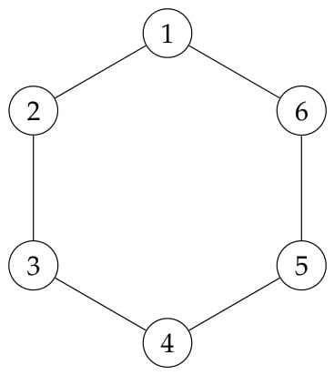
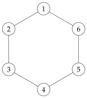
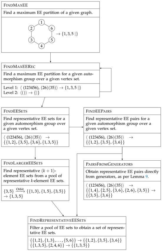
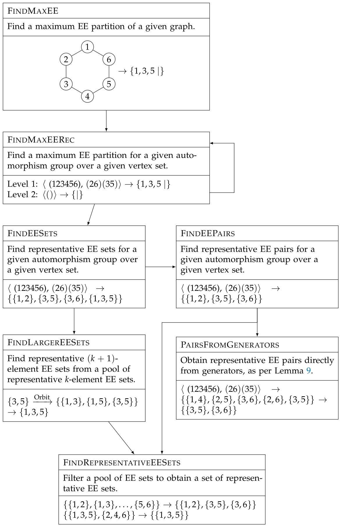
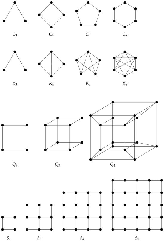
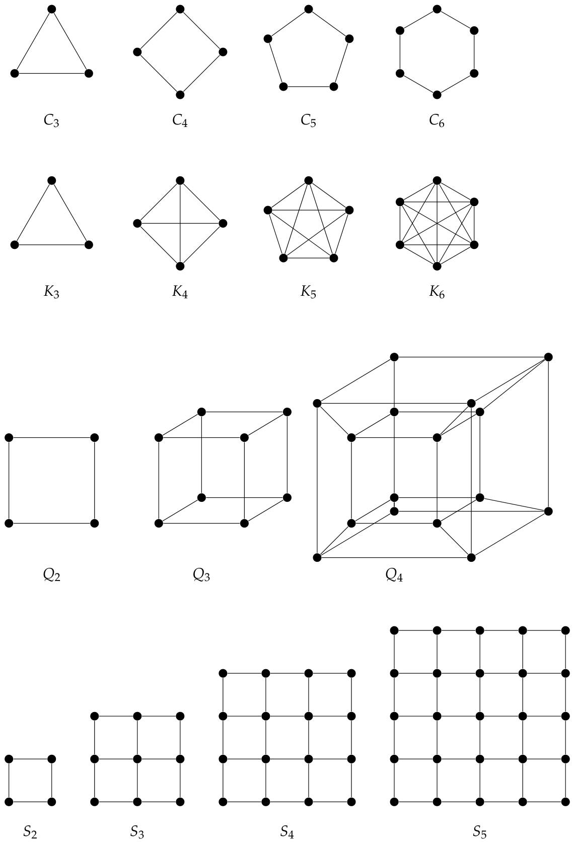
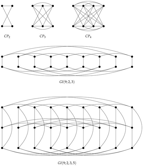
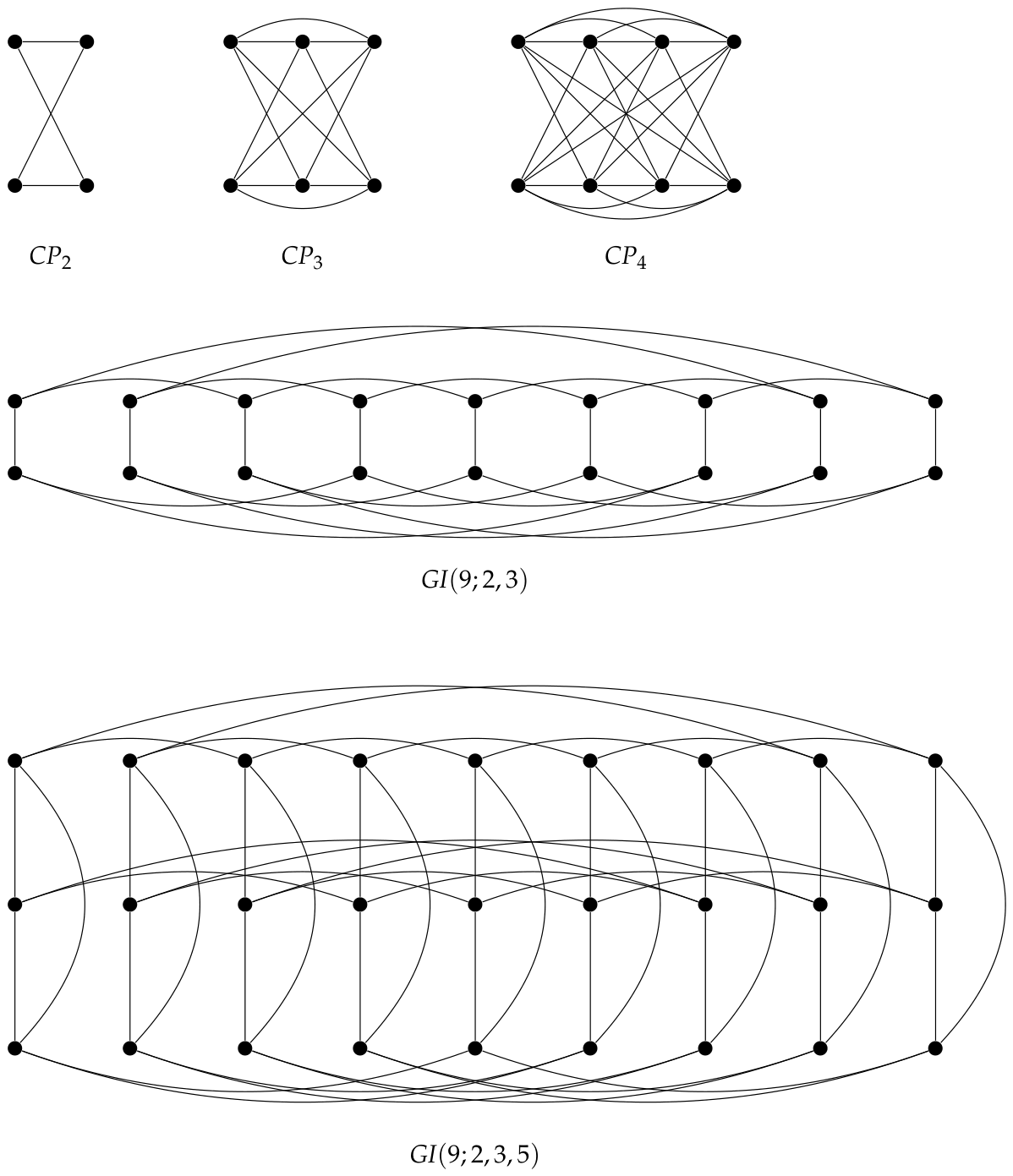
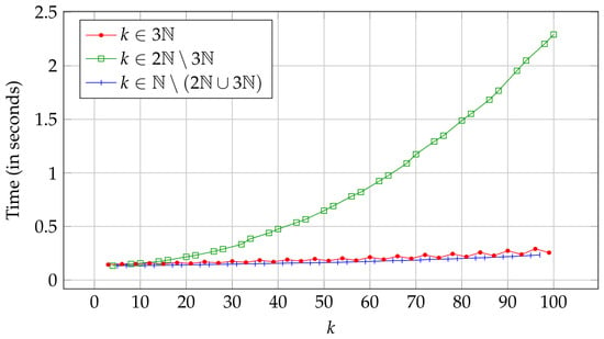
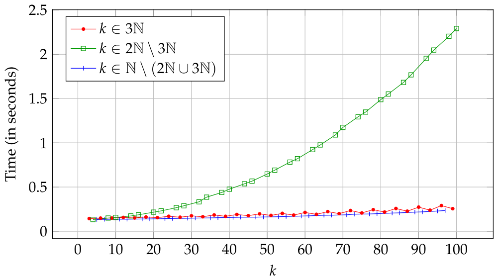
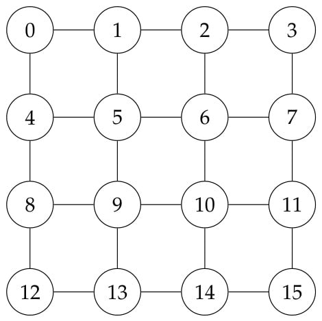
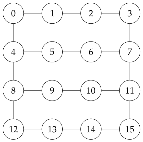
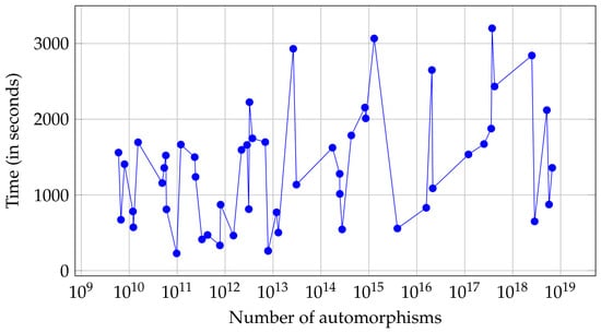
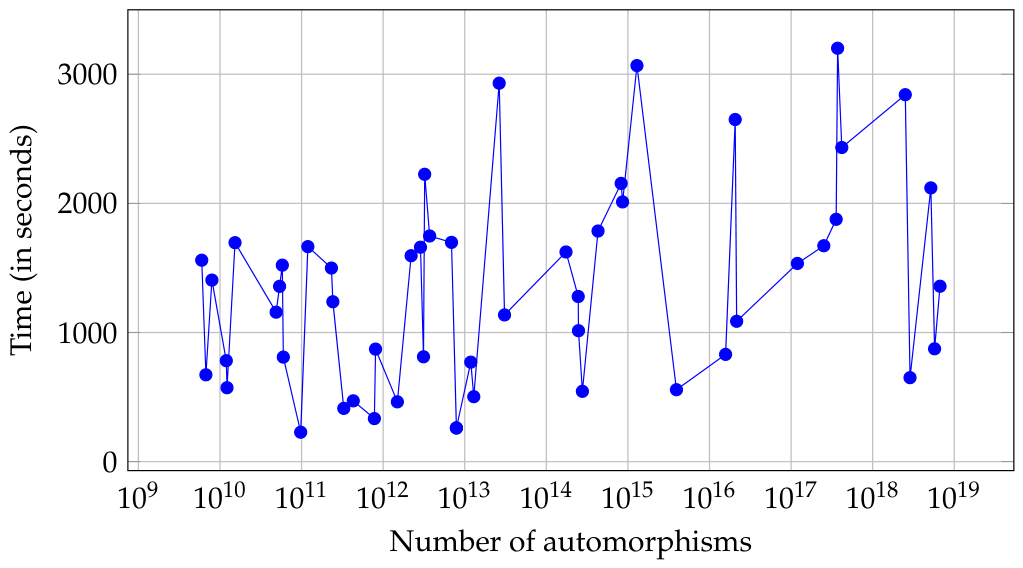
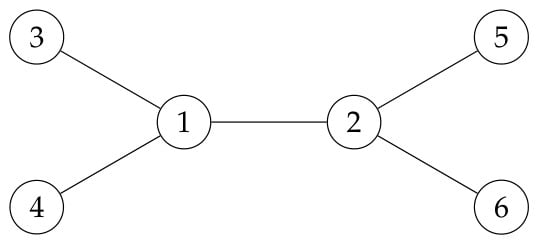
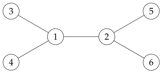

Disclaimer/Publisher’s Note: The statements, opinions and data contained in all publications are solely those of the individual author(s) and contributor(s) and not of MDPI and/or the editor(s). MDPI and/or the editor(s) disclaim responsibility for any injury to people or property resulting from any ideas, methods, instructions or products referred to in the content. |
© 2026 by the authors. Licensee MDPI, Basel, Switzerland. This article is an open access article distributed under the terms and conditions of the Creative Commons Attribution (CC BY) license.