


Abstract
This short review discusses recent applications of Reinforcement Learning (RL) techniques to the flavor problem in particle physics. Traditional approaches to fermion masses and mixing often rely on extensions of the Standard Model based on horizontal symmetries, but the vast landscape of possible models makes systematic exploration infeasible. Recent works have shown that RL can efficiently navigate this landscape by constructing models that reproduce observed quark and lepton observables. These approaches demonstrate that RL not only rediscovers models already proposed in the literature but also uncovers new, phenomenologically acceptable solutions.
1. Introduction
The flavor problem in particle physics has been a central focus of study since the inception of the Standard Model (SM). Many attempts to explain fermion masses and mixing involve SM extensions based on horizontal symmetries, which relate the entries of the mass matrices in a non-trivial way rather than treating them as free parameters. A common feature of all these models is the assignment of particles to irreducible representations of the flavor group (the case of non-abelian symmetries), the assignment of a charge to particles (models á la Froggatt–Nielsen [1]) or a combination of both. The space of all possibilities is usually immense, spanning ∼ different models, with n a large integer of . It is clear that the success of an SM extension strongly relies on the ability to select a realization that fits the low energy data; although searches carried out by humans have produced viable solutions, it remains unclear whether these are minimal in terms of the required new degrees of freedom, or optimal with respect to other criteria, such as avoiding large hierarchies in the model parameters or the need for strong fine-tuning. The vastness of the parameter space in many fields of particle physics is one of the reasons why, in very recent years, Machine Learning (ML) techniques started to be applied to several problems in Physics. Entering into the details of all attempts performed using ML techniques in Physics is a formidable task, as in many areas a long list of papers exist and revising them is well beyond the scope of this short review. In the restricted domain of theoretical physics, the subject is currently very active, covering a wide range of topics ranging (among others) from string theory [2,3,4,5,6,7,8,9,10,11,12,13,14,15,16,17,18,19,20,21,22,23,24,25,26,27,28,29,30,31,32,33,34] to QCD [35,36,37,38,39,40,41,42,43,44,45,46,47,48,49,50,51,52,53,54,55,56,57,58,59,60], not to mention statistical mechanics [61,62,63,64,65,66,67,68,69,70,71,72,73,74,75,76,77,78,79,80,81,82,83,84,85,86,87,88], thermodynamics [89,90,91,92,93], the foundation of quantum mechanics [94,95,96,97,98,99,100,101,102], and cosmology [103,104,105,106,107,108,109,110,111,112,113,114,115,116,117,118,119]. In this short review, we focus more strictly on ML in particle physics [120,121,122,123,124], with the intent of exploring beyond the Standard Model theories [125,126,127] and, in particular, the efforts (a few, so far) that have been made to implement AI agents in the study of the flavor problem. The subject is relatively young, so, at least in principle, there exists a large probability that more can be said and done in the near future. This review would help in setting the state of the art on the attempts accomplished using the Reinforcement Learning (RL) technique [128] to find promising quark [129] and lepton [130,131] textures. (Note 1: A study based on the Diffusion Model (DF) has been carried out for leptons [132]) addressing, at the same time, the quest for an axion candidate. More generally, the same RL-based strategy can be straightforwardly adapted to other areas of particle physics, such as to problems in theoretical physics where model building amounts to exploring large, discrete or continuous spaces under theoretical and phenomenological constraints. Among others, we mention string theory [133], particle jets physics [134], lattice QCD [135], and quantum field theory [136,137].
2. Reinforcement Learning
Reinforcement Learning [128] is a subfield of Machine Learning that focuses on how an agent learns to make optimal decisions by interacting with an environment to maximize a cumulative reward over time. Unlike supervised learning, which trains on labeled input-output pairs, and unsupervised learning, which seeks patterns in unlabeled data, RL operates in a trial-and-error framework, analogous to a human strategist attempting to master a complex task. The agent learns by taking actions, observing their consequences, and receiving feedback in the form of rewards or penalties. This feedback loop allows the agent to gradually refine its decision-making strategy without being explicitly told what the “correct” action is. This continuous refinement process, based on performance feedback rather than explicit instruction, mirrors how humans develop expertise in complex domains. This paradigm is well-suited to problems in which the optimal course of action is not immediately clear and the agent must explore its environment to discover effective strategies. RL is often formalized using Markov Decision Processes (MDPs), which provide a mathematical framework for modeling sequential decision-making under uncertainty. In RL, the agent observes the current state of the environment, selects an action, and receives a reward along with the next state, iteratively learning a policy—a strategy that maps states to actions—to maximize the expected sum of future rewards.
Common Features
Although many variants of RL exist, we can identify some common features; these components are essential for understanding how RL systems operate:
- Agent: the entity responsible for making decisions and learning from experience. The agent could be a robot, a software program, or any system capable of taking actions in an environment;
- Environment: the external system with which the agent interacts. The environment includes everything outside the agent, such as a physical space, a game board, or a simulated market. It responds to the agent’s actions by providing new states and rewards;
- State (): a representation of the current situation or configuration of the environment at a given time. The state contains all the relevant information the agent needs to make a decision. For example, in a chess game, the state could represent the positions of all pieces on the board. With , we indicate the ensemble of the whole states, whose single realization is indicated with s;
- Action (): a decision or move the agent can make to influence the environment. Actions can be discrete (e.g., moving left or right) or continuous (e.g., adjusting the speed of a vehicle). The set of all possible actions depends on the environment and the current state;
- Reward (): a scalar value provided by the environment after each action, indicating the immediate benefit or cost of that action. The reward serves as feedback, guiding the agent toward desirable behaviors. For instance, a positive reward might be given for winning a game, while a negative reward (penalty) could be assigned for making an invalid move in a chess game;
- Policy (): the strategy or rule that the agent follows to select actions based on the current state. Formally, a policy is a mapping from states to actions, denoted as (for deterministic policies) or (for probabilistic policies, which assign probabilities to actions given a state). The goal of RL is to learn an optimal policy that maximizes long-term rewards;
- Value Function (): a function that estimates the expected cumulative reward (also called the return) an agent can achieve starting from a given state s and following the policy . The value function quantifies the long-term desirability of a state under a specific policy. A related concept is the action-value function (), which estimates the expected return for taking action a in state s and following policy afterward. Notice that the reward r and the value function are fundamentally related: the reward provides the immediate feedback signal, while the value function is the estimation of the long-term benefit derived from those rewards.
- Discount Factor (): a parameter that determines the importance of future rewards relative to immediate ones. A value of close to 0 prioritizes short-term rewards, while a value close to 1 emphasizes long-term rewards, promoting long-term planning by the agent.
- Learning Rate (): a parameter which controls how much newly acquired information overrides old information when updating estimates. When is close to 1, the agent quickly adapts to new experiences but tends to forget past knowledge; conversely, for close to 0, the agent learns slowly, giving more weight to prior knowledge and less to new data. It can decay over time, making updates smaller as learning converges.
As mentioned above, RL problems are typically formalized as MDPs, which provide a structured framework for modeling sequential decision-making in environments with stochastic dynamics. An MDP is defined by a tuple , where and have been defined above, and is the transition probability function, which specifies the probability of transitioning from the current state s to a new state after taking action a.
The objective of RL is to find an optimal policy that maximizes the expected discounted return, defined as the expected sum of discounted rewards over an infinite horizon [128]:
Here, represents the return starting from time step t, which is the total discounted reward accumulated by following policy . To achieve this goal, RL algorithms often rely on two key approaches:
- Value-based methods: these methods estimate the value function ( or ) and derive a policy by selecting actions that maximize the estimated value. A classic example is Q-learning, which iteratively updates the action-value function to learn an optimal policy without explicitly modeling the environment’s transition dynamics [138]. At the heart of Q-learning is the Bellman equation used to update Q-values:where is the current state at time t; is the action taken at time t; is the reward received after taking action ; is the new state after taking action ; is the learning rate; is the discount factor; and is the estimate of the maximum future reward from the next state. In this procedure, one first initializes the Q-table arbitrarily for all state-action pairs ; then, choose an action a from state s using a policy (e.g., -greedy (Note 2: Q-learning balances exploration and exploitation typically using an -greedy policy: with probability , choose a random action and with probability , choose the action that maximizes the current Q-value.)) takes action a, as well as observes reward r and the next state . Then, the Q-value is updated as follows:and one sets . The goal is to find the optimal Q-function such that:where the symbol defines the expected value. In other words, the optimal value of taking action a in state s equals the expected value of the immediate reward plus the discounted () value of the best possible future action in the next state . The term “” indicates that, in the future, the agent will always select the best action.Once is learned, the optimal policy can be derived as follows:Notice that, while gives the maximum value of the function over all possible actions a, with the notation we denote the function that returns the action a that achieves this maximum value.
- Policy-based methods: These methods directly parameterize and optimize the policy , where are tunable parameters of the policy (e.g., weights of a neural network) [139]. Instead of estimating a value function first, policy-based methods adjust to maximize the expected return:The gradient of with respect to the parameters can be estimated using sampled trajectories from the environment. A prototypical algorithm is REINFORCE, which updates the parameters in the direction of the return:where is the cumulative discounted reward from time t defined in Equation (1). REINFORCE is suitable for RL because it estimates the policy gradient from sampled trajectories without requiring a model of the environment. However, its gradient estimates have high variance, often necessitating variance-reduction techniques for stable and efficient learning.Policy-based methods naturally handle high-dimensional or continuous action spaces and can learn stochastic policies, which are useful in partially observable or highly uncertain environments.
There also exist hybrid approaches called actor-critic methods, which combine value-based and policy-based ideas by learning both a value function (critic) and a policy (actor) to improve sample efficiency [140].
In the following section, we review attempts to address the flavor problem using RL techniques.
3. Quark and Lepton Masses and Mixing from RL
3.1. Froggatt–Nielsen for Quark Observables
The first paper we want to discuss is Ref. [129], which explores the application of RL to model building, explicitly focusing on Froggatt–Nielsen (FN) type models for quark masses and mixing. The primary goal is to investigate whether RL techniques can be used to train a neural network [141] to construct particle physics models with specific prescribed properties. More specifically, the authors aimed to develop a system in which an RL agent could efficiently transition from random, typically physically unacceptable FN models to phenomenologically viable ones consistent with observed quark masses and mixing. In addition, they also wanted to test whether the trained networks could not only discover new models but also identify models already proposed in the literature.
From the model-building point of view, FN models are well known and, for the present paper, work as follows. In the Standard Model (SM), quark masses and mixings originate from Yukawa couplings:
where are left-handed quark doublets, and are right-handed up- and down-type quarks, and H is the Higgs doublet. After electroweak symmetry breaking, the Higgs acquires a VEV , yielding the mass matrices:
These are diagonalized via unitary matrices:
with and . The observable mixing is encoded in the CKM matrix:
parameterized by three angles and a CP-violating phase :
The experimentally measured parameters used in the paper are shown in Table 1 for reference.
Table 1.
Reference values of the quark masses (in GeV) and CKM parameters used in [129].
FN models introduce a flavor structure into the SM via two main ingredients:
- adding global symmetries , to the SM gauge group;
- adding scalar singlets , with responsible for the spontaneous breaking of ’s.
The SM Yukawa terms are generally replaced by higher-dimensional operators:
where ; if the sum of all charges in a given operator is vanishing, then the related entries in the Yukawa matrix are different from zero. After the singlets acquire VEVs , the Yukawa matrices become:
where are coefficients not determined by the flavor symmetries and fixed to some random number at the beginning of the simulation. In this framework, an FN model is defined by vectors
organized into an charge matrix , where r is the number of symmetries, with bounded entries
for each particle in the model. The Higgs charges have been fixed to ensure the top Yukawa coupling is unsuppressed:
The FN landscape consists of many possible charge assignments. For example, with one and , there are models; for two symmetries, ∼. Identifying viable models matching experimental data motivates the use of RL techniques. The setup involves a single neural network , parameterized by weights , which defines the policy . The network takes states as input and outputs a probability distribution over possible actions. Exploration of the environment is driven by this policy, meaning actions are sampled according to at each step in an episode, defined as the sequence of states and actions for (the maximum t representing the length of the episode):
Data is collected by repeatedly running such episodes, implying that the system effectively consists of a single agent. According to the policy gradient theorem, the policy network is trained to minimize the following loss function:
In practice, the action-value function is often approximated using the return G observed from state s. The overall algorithm proceeds as follows:
- (1)
- Initialize the policy network .
- (2)
- Collect a batch of data tuples by running multiple episodes as described in (18), with each episode starting from a randomly selected initial state .
- (3)
- Update the policy network parameters using the collected data and the loss function in (19).
- (4)
- Repeat steps (2) and (3) until convergence, i.e., when the loss becomes sufficiently small, and the policy stabilizes.
The authors model the FN theory space as an MDP. The state space consists of all FN charge matrices of Equation (15). The action space is composed of elementary updates that increment or decrement a single charge by one, that is . Since these updates are deterministic, the transition probabilities are not needed. There are such actions in total. The discount factor is fixed to .
In order to define a reward function, the authors first introduce the intrinsic value of a state , defined as follows:
where the minimization is over scalar VEVs (with typical values and ) and runs over the six quark masses and CKM elements. This quantity measures the total deviation of the model predictions from the experimental values. In this context, a terminal state (that is a state after which the episode ends and a new one starts) satisfies , and all individual deviations (defined as computed for the value for which is minimum) are greater than , with and . Thus, a reward function is defined by the following:
with . The training is performed using the REINFORCE algorithm (described in the previous section) with ADAM optimization (Note 3: ADAM is an optimization method that automatically adjusts how big each training step should be by keeping track of both the average direction of past steps (momentum) and how much those steps vary (adaptive learning rate), making it faster and more stable for training models). A single agent explores the FN environment using the policy , running episodes of maximum length starting from random initial states. Terminal states discovered during training are stored for further analysis. For models with one symmetry, the trained network leads from random initial configurations to phenomenologically acceptable models in 93% of episodes, with an average episode length of 16.4. On the other hand, for models with two symmetries, the network achieved a success rate of 95% of episodes ending in terminal states. The average episode length in this more complex scenario was ∼20. In particular, 4630 unique terminal states were found for the one symmetry case. Among these, 89 models had a high “intrinsic value” (meaning they fit experimental data well), with the best achieving a value of approximately . 57,807 unique terminal states were discovered for the two symmetries case. Of these, 2019 models showed high intrinsic value, with the best model having a value of approximately . Models with the highest intrinsic value for one and two symmetries have been reported in Table 2. The training process, even for the larger two symmetry environment, was achieved on a single CPU within reasonable timeframes of 1 h for one symmetry, and 25 h for two symmetries, demonstrating the practical applicability of RL for navigating large model spaces where systematic scanning is impossible. It is worth noting that the trained networks were shown to guide the search toward FN models previously proposed in the literature, provided that the search started from a nearby configuration in the model space.
Table 2.
Examples of models with the highest intrinsic value for one (top) and two (bottom) symmetries. Charges and coefficients of Equation (13) are given. Adapted from [129].
Even though not strictly related to FN models, we want to mention here the efforts provided in [8] where machine learning techniques have been applied to construct particle physics models again in the Yukawa quark sector, aiming to satisfy two complementary criteria: truth and beauty. Truth is defined as the ability of a model to reproduce all experimental observables sensitive to its parameters. In the quark sector, this entails fitting quark masses and mixing parameters, including the CKM matrix elements and the Jarlskog invariant. Beauty (Note 4: The implementation of the beauty definitions in the context of machine learning approaches to BSM models in flavor physics might be useful to narrow down the viable models in order to search for the most theoretically appealing solutions), in the authors’ definition, refers to desirable theoretical attributes beyond mere data fitting. To quantify beauty in Yukawa matrices, three measures are tested, which are uniformity (that is, all matrix elements have approximately equal magnitude), sparsity (where a significant number of elements vanish exactly or are negligibly small), and symmetry (in which off-diagonal elements are mirrored in magnitude across the main diagonal). Using pseudo-experiments, the optimization procedure efficiently navigates the vast parameter space, uncovering models that achieve both experimental accuracy and aesthetic elegance. This effort demonstrates how machine learning can be applied in particle physics, not only as an efficient method for exploring vast parameter spaces but also as a flexible tool for model selection (accounting for theoretical and phenomenological constraints), thereby bridging numerical optimization and model-building intuition.
3.2. Extension of the Froggatt–Nielsen to Lepton Observables
We now discuss the paper [130], which extends the previous work to investigate the flavor structure not only for quarks but also for leptons using RL. Specifically, the authors apply a value-based RL algorithm to models with a flavor symmetry based on the Froggatt–Nielsen (FN) mechanism. While, as said, for charges in the range to quarks alone yields approximately possible configurations, the inclusion of the lepton sector expands the parameter space to over possibilities. This combinatorial explosion renders brute-force searches infeasible and motivates the application of machine learning techniques for efficient model exploration. The system is provided with the following components:
- Deep Q-Network (DQN): a DQN implementation has been supplied to approximate the Q-value function, guiding the agent’s actions via a neural network. In fact, instead of storing a Q-table, the DQN uses a neural network to approximate the Q-function. It leverages experience replay (learning from past transitions randomly sampled from memory) to break correlations between consecutive experiences, and incorporates a target network to stabilize training by maintaining a delayed copy of the Q-network for computing target values.
- Network Architecture: The architecture of each network is composed of several fully connected (dense) layers, where each neuron in a layer is connected to every neuron in the subsequent layer. The activation function used in these layers is the Scaled Exponential Linear Unit (SELU), which helps maintain normalized activations and supports stable training. The final layer of the network uses a softmax activation (that is, a function that converts raw outputs into probabilities summing to one) to produce a probability distribution over the possible actions.
As before, the training procedure is implemented, first, by inputting the current state s (a charge vector ) into the target network; then, actions a are chosen via an -greedy policy (see Note 2). After that, the transition (where is the reward received by the agent, more on this later) is stored in a replay buffer. A mini-batch of experiences is sampled to update the Q-network using a Huber loss function, optimized via stochastic gradient descent. The Huber loss function is an error measure that combines the advantages of the mean squared error (MSE) and the mean absolute error (MAE). For small differences between the predicted value and the target value y, it behaves like MSE, while for large differences, it behaves like MAE, increasing its numerical stability while still being sensitive to small errors. Denoting the outputs of the Q-network and the target network by and , respectively, the weights and the biases are updated by minimizing the following:
with and , which combines a mean squared error and a mean absolute error.
At the end, the Q-network parameters are softly copied to the target network parameters using a learning rate . The models investigated by the authors are built with a single complex scalar flavon field with a charge. As usual, Yukawa couplings are suppressed by powers of , generating fermion mass hierarchies. In addition, the Higgs charge is fixed to allow the top Yukawa term without flavon suppression. The resulting fermion masses and mixings arise after , and the Higgs acquire VEVs: and . The total charge vector contains 19 components (for all fermions); each component lies within , leading to ∼ possible charge configurations, as previously anticipated. The flavon charge is set to or with equal probability. Agent actions consist of incrementing or decrementing a component of by one unit.
The relevant Yukawa terms for leptons (those for quarks are analogous to the previous section) are given by the following:
where denote the left-handed leptons, the right-handed charged leptons, the right-handed neutrinos, and the SM Higgs doublet with , respectively. In the paper, the authors assume three right-handed neutrinos and that the physical neutrino masses are generated by the Type-I seesaw mechanism, where the large mass M is chosen as GeV and the Yukawa couplings (including those for u and d quarks) are real coefficients.
The reward is based on an intrinsic value function , which quantifies how well a charge configuration reproduces the observed fermion masses and mixing angles:
In Equation (24), and measure the deviation of the predicted quark and lepton masses from their corresponding experimental values,
where
In addition, since the ordering of neutrino masses is not yet experimentally established, they considered two approaches: RL with a fixed ordering (either Normal Ordering (NO) or Inverted Ordering (IO)) and RL without specifying the ordering. The intrinsic value relevant to the neutrino masses is given by the following:
with . Finally, the intrinsic value also incorporates quark and lepton mixing information through the quantities where
The experimental values of the lepton observables used by the authors are listed in Table 3.
Table 3.
Experimental values for the lepton sector obtained from global analysis of the data, where for NO and for IO. Taken from [130].
A configuration is considered a terminal state if
with typical thresholds , , and .
In the quark sector, approximately configurations were explored. After ∼15 h on a single CPU, the agent reached terminal states after 20,000 episodes. More than 6% of 100,000 episodes reached valid terminal states; 21 independent charge configurations consistent with experimental data were identified. Monte Carlo optimization of Yukawa coefficients refined the results to fit within <0.1% of observed values. However, as the authors claim, no CP violation is present in this sector due to the phase-rotation freedom.
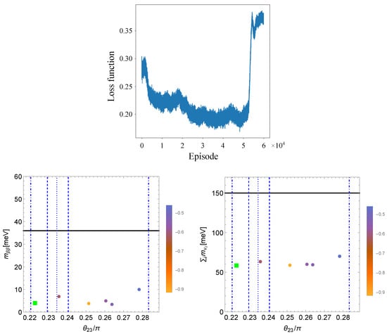
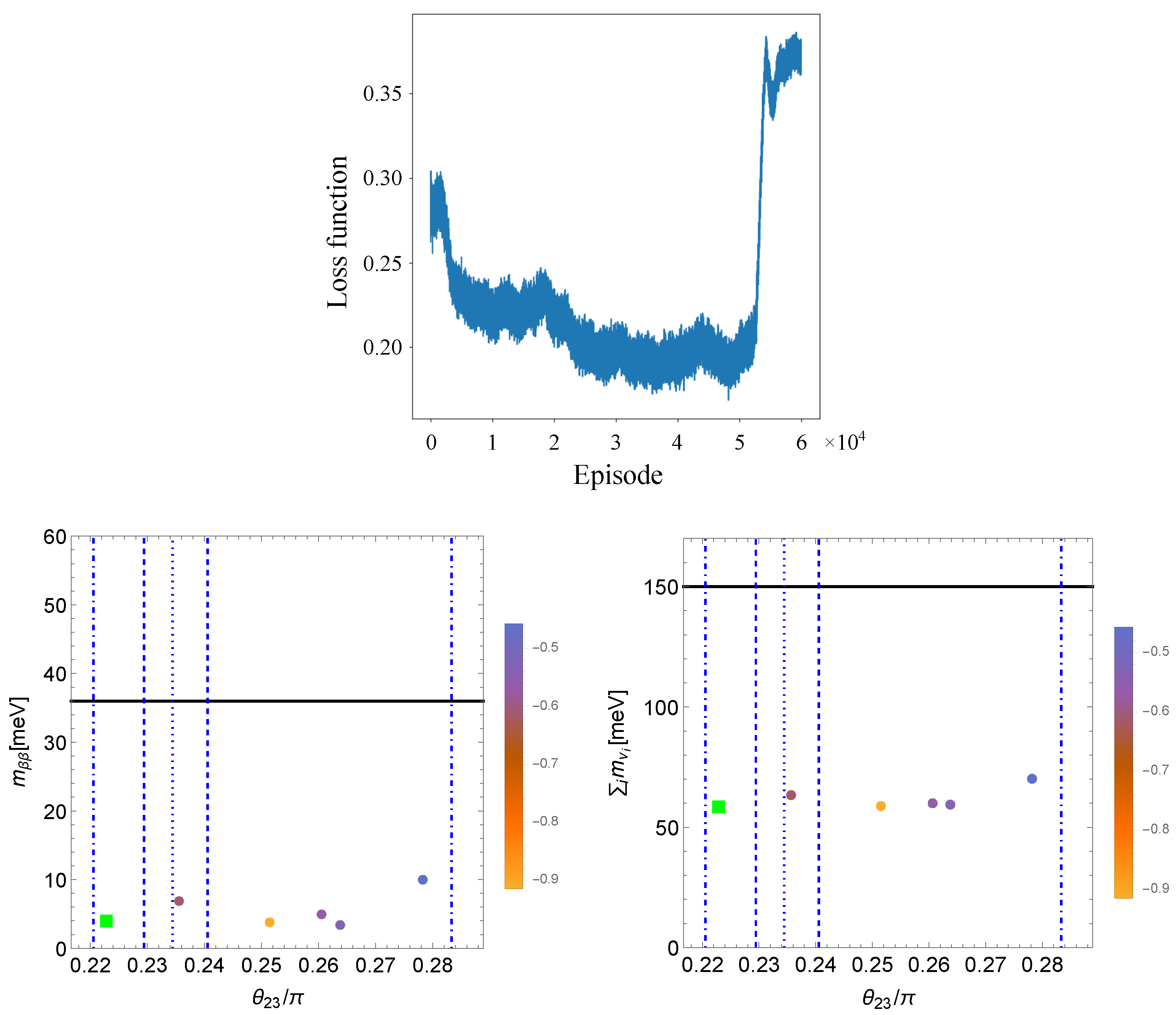
In the lepton sector, the authors analyzed models in two different situations of mass ordering, one in which the ordering is fixed a priori and another when it is left free to be chosen by the agent’s action. For both cases, the Higgs charges and flavon VEVs were fixed from the quark sector. In the case of fixed mass ordering, the training started to find terminal states after roughly 5000 episodes (around 8 h on a single CPU) while the loss function tended to be minimized around 50,000 episodes (see the upper panel of Figure 1.)
Figure 1.
Learning results for the lepton sector by RL, having specified the neutrino mass ordering. Upper panel: loss function vs. episode number. Lower panels: effective neutrino mass (left plot) and sum of the neutrino masses (right plot) versus the atmospheric mixing angle , for the six viable models found by the authors. See text for further details. Adapted from [130].
Here, the horizontal axis shows the number of training episodes, while the vertical axis reports the value of the loss function. A decreasing trend with fluctuations can be observed, indicating that the agent is gradually improving its predictions, with variations arising from the stochastic nature of the learning process. After ∼ episodes, the loss no longer decreases; instead, it slightly rises, suggesting potential overfitting to the specific experiences in the replay buffer. In particular, terminal states appeared in 0.06% of the cases: 63 (NO) and 121 (IO) total. Monte Carlo scans revealed six viable models for NO within 3, while no valid models for IO were found. These results suggest that NO is statistically preferred. A typical successful output with a large intrinsic value is reported in Table 4, together with the lepton and scalar charges, the Yukawa matrices, the flavon vev, the obtained PMNS matrix, and the predictions for the Majorana phases and .
Table 4.
Highest intrinsic value scenario for the lepton sector with NO, where the neutrino mass ordering is specified in the network training. Adapted from [130].
For the sake of completeness, in the lower panels of Figure 1, we report the effective neutrino mass (left plot) and the sum of the neutrino masses versus the atmospheric mixing angle (right plot) for the six viable models found by the authors. In the last two plots, the dotted line represents the global best fit value from NuFIT v5.2 results with Super-Kamiokande atmospheric data [142], while the region inside the dashed (dot-dashed) line corresponds to () confidence level interval. The square corresponds to the model listed in Table 4. The left panel shows that the predicted effective Majorana neutrino masses are all around a factor of 4 below their upper bound of 36 meV (90% CL) indicated by the black solid line [143]; from the right panel, instead, we see that the sum of neutrino masses are all roughly 3 times smaller than the upper bound of 15 meV (95% CL), corresponding to the black solid line in the case of CDM model [144].
In the case of unfixed mass ordering, the training took ∼12 h, and terminal states were found in over 60% of 60,000 episodes. In two dedicated runs, the authors found more that 13 k terminal states for NO and 22 k for IO. After optimization of the (1) coefficients, 15 NO models matched observations within 3, while, again, no IO models were viable. This work demonstrates that reinforcement learning can effectively explore the flavor structure of fermions in models with symmetry. The results strongly suggest that Normal Ordering is statistically favored over Inverted Ordering in the neutrino sector.
3.3. An AI Agent for Autonomous Model Building
As a step forward in response to the challenges posed by the flavor problem in the sector, the authors of [131] introduce the Autonomous Model Builder (AMBer), an AI-assisted framework based on RL. AMBer is designed to efficiently navigate the vast combinatorial landscape of model-building possibilities. In its implementation, the system autonomously selects symmetry groups, defines particle content, assigns group representations, and evaluates the resulting models. The goal is to construct viable models that both minimise the number of free parameters and reproduce experimental observations. While the framework has been demonstrated in the context of neutrino flavor mixing, the underlying methodology is general and can be adapted to other domains of theoretical physics.
In the paper, the problem of constructing neutrino flavor models is reformulated as an RL task. The environment in which the RL agent operates is defined by the space of possible models, with the current state corresponding to a specific model under consideration. Actions correspond to modifications of the model, such as altering particle content, changing group representations, or modifying symmetry properties, subject to mathematical consistency conditions. Each particle is encoded via a one-hot vector reflecting its non-Abelian representation and Abelian charge, while additional state information includes lepton triplet associations, vacuum expectation value configurations for flavons, and the order of the Abelian symmetry.
The agent evaluates its performance using a reward function carefully designed to encourage models that achieve a good fit to data, minimize the number of free parameters, and explore higher-order Abelian symmetries when advantageous. Invalid actions or models are penalized, while valid and predictive configurations are rewarded. The reward is normalized between and 1, with high-quality states boosted to maximize their influence on learning.
To enable rapid model evaluation, the framework incorporates an optimized software pipeline. A Python reimplementation of the Mathematica Discrete package, PyDiscrete, computes Clebsch–Gordan coefficients with substantial speed gains. The Model2Mass package symbolically constructs the superpotential and extracts the charged-lepton, Dirac neutrino, and Majorana mass matrices for arbitrary finite non-Abelian groups. For parameter fitting, the FlavorPy package is employed, performing multiple short optimisation runs from varied initial conditions to avoid local minima while keeping computational costs low.
The RL algorithm chosen for AMBer is Proximal Policy Optimisation (PPO), which learns a policy directly and updates it carefully to avoid significant changes at once. It uses a value function to assess the quality of actions, learns only from data generated by its current behavior, and employs advantage estimates to stabilize learning. By reusing the same data for a few updates, PPO achieves reliable learning without becoming unstable. The loss function includes value, policy, and entropy terms, balancing exploitation and exploration. Training is performed in parallel over 250 environments, each with a maximum episode length of 1000 steps. Model evaluation occurs every few steps, with the frequency depending on the chosen symmetry group. The search is conducted across several theory spaces, including with up to five flavons, with variable N, and with up to six flavons.
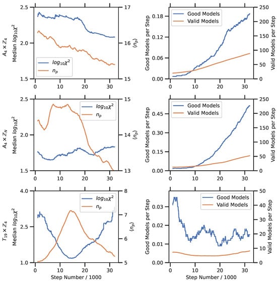
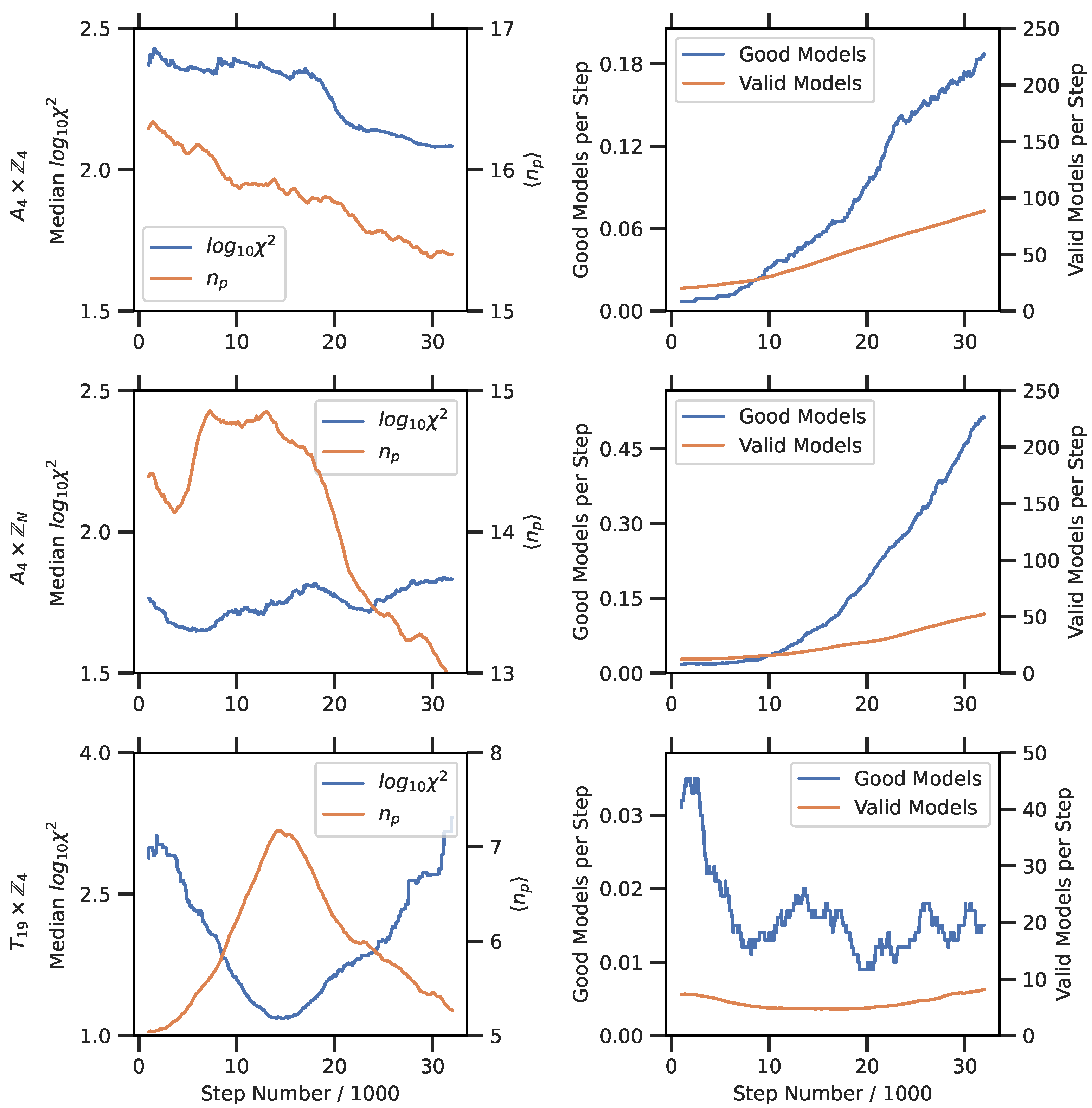
Throughout training, the agent’s performance is monitored by tracking the fit to data, the number of free parameters, and other internal metrics, see Figure 2.
Figure 2.
Training variables of interest over time for searches in three spaces: (top), (middle), and (bottom). Left column: evolution of in blue (where the curve indicates the median over all environments) and the mean number of parameters as training progresses in orange. Right column: number of valid models in orange and good ( and 7) models in blue. From [131].
Comparisons with random scans reveal that AMBer significantly outperforms naive exploration strategies, particularly in the -based theory spaces.
The application of AMBer to neutrino flavor model building yields thousands of models that are both predictive (having at most seven free parameters) and in good agreement with experimental data, with . In the search space, many of the models rediscovered align closely with known constructions from the literature, featuring typical triplet assignments for lepton doublets and right-handed neutrinos, along with favored vacuum alignments such as . The runs (see Table 5 for a typical output) demonstrate the agent’s flexibility in selecting symmetry orders.
Table 5.
Model found by AMBer in the search (with ), with 5 parameters and . Here .
In the larger and less charted theory space, AMBer uncovers models with more uniform representation assignments and an expanded variety of viable structures. Although the relative gain over random scans is smaller here, AMBer still identifies more good models, including particularly simple configurations with very few free parameters.
4. Conclusions
In this short review, we summarize the first applications of Reinforcement Learning (RL) to the flavor problem in particle physics. Traditional approaches to quark and lepton mass hierarchies face the challenge of exploring a vast model space, which quickly becomes intractable as symmetries and parameters increase. RL-based frameworks have demonstrated the ability to efficiently navigate these spaces, identifying viable Froggatt–Nielsen charge assignments for quarks and leptons, often rediscovering known models and, in some cases, uncovering new ones consistent with experimental data. In the lepton sector, RL results indicate a statistical preference for the Normal Ordering of neutrino masses. More advanced frameworks, such as AMBer, further illustrate the potential of AI agents to autonomously construct Beyond Standard Model theories with minimal parameter dependence and predictive power. Although this field is still in its infancy, the promising results obtained so far indicate that RL may become a valuable tool in theoretical model building, complementing traditional approaches and opening new directions in the search for solutions to the flavor problem, as those based on modular symmetries and non-holomorphic modular forms.
In the future, we expect RL to have a significant impact on the development of fully autonomous theory-design frameworks, and its ability to explore more complex parameter spaces compared to simple random scans will be clarified.
Funding
This research received no external funding.
Data Availability Statement
No new data were created or analyzed in this study. Data sharing is not applicable to this article.
Conflicts of Interest
The authors declare no conflicts of interest.
References
- Froggatt, C.D.; Nielsen, H.B. Hierarchy of Quark Masses, Cabibbo Angles and CP Violation. Nucl. Phys. B 1979, 147, 277–298. [Google Scholar] [CrossRef] [Scilit]
- Halverson, J.; Nelson, B.; Ruehle, F. Branes with Brains: Exploring String Vacua with Deep Reinforcement Learning. J. High Energy Phys. 2019, 2019, 3. [Google Scholar] [CrossRef] [Scilit]
- Mütter, A.; Parr, E.; Vaudrevange, P.K.S. Deep learning in the heterotic orbifold landscape. Nucl. Phys. B 2019, 940, 113–129. [Google Scholar] [CrossRef] [Scilit]
- He, Y.H. Deep-Learning the Landscape. arXiv 2017, arXiv:1706.02714. [Google Scholar] [CrossRef] [Scilit]
- Krefl, D.; Seong, R.K. Machine Learning of Calabi-Yau Volumes. Phys. Rev. D 2017, 96, 066014. [Google Scholar] [CrossRef] [Scilit]
- Ruehle, F. Evolving neural networks with genetic algorithms to study the String Landscape. J. High Energy Phys. 2017, 2017, 38. [Google Scholar] [CrossRef] [Scilit]
- Abel, S.; Rizos, J. Genetic Algorithms and the Search for Viable String Vacua. J. High Energy Phys. 2014, 2014, 10. [Google Scholar] [CrossRef] [Scilit]
- Matchev, K.T.; Matcheva, K.; Ramond, P.; Verner, S. Exploring the truth and beauty of theory landscapes with machine learning. Phys. Lett. B 2024, 856, 138941. [Google Scholar] [CrossRef] [Scilit]
- Larfors, M.; Schneider, R. Explore and Exploit with Heterotic Line Bundle Models. Fortsch. Phys. 2020, 68, 2000034. [Google Scholar] [CrossRef] [Scilit]
- Krippendorf, S.; Kroepsch, R.; Syvaeri, M. Revealing systematics in phenomenologically viable flux vacua with reinforcement learning. arXiv 2021, arXiv:2107.04039. [Google Scholar] [CrossRef] [Scilit]
- Constantin, A.; Harvey, T.R.; Lukas, A. Heterotic String Model Building with Monad Bundles and Reinforcement Learning. Fortsch. Phys. 2022, 70, 2100186. [Google Scholar] [CrossRef] [Scilit]
- Cole, A.; Krippendorf, S.; Schachner, A.; Shiu, G. Probing the Structure of String Theory Vacua with Genetic Algorithms and Reinforcement Learning. arXiv 2021, arXiv:2111.11466. [Google Scholar] [CrossRef] [Scilit]
- Seong, R.K. Generative AI for brane configurations and coamoeba. Phys. Rev. D 2025, 111, 086013. [Google Scholar] [CrossRef] [Scilit]
- Harvey, T. Navigating the String Landscape with Machine Learning Techniques. Ph.D. Thesis, Oxford University, Oxford, UK, 2024. [Google Scholar] [CrossRef]
- Lanza, S. Neural network learning and Quantum Gravity. J. High Energy Phys. 2024, 2024, 105. [Google Scholar] [CrossRef] [Scilit]
- Choi, E.; Seong, R.K. Machine learning regularization for the minimum volume formula of toric Calabi-Yau 3-folds. Phys. Rev. D 2024, 109, 046015. [Google Scholar] [CrossRef] [Scilit]
- Hirst, E. Machine-Learning and Data Science Techniques in String and Gauge Theories. Ph.D. Thesis, University of London, London, UK, 2023. [Google Scholar]
- Cui, W.; Gao, X.; Wang, J. Machine learning on generalized complete intersection Calabi-Yau manifolds. Phys. Rev. D 2023, 107, 086004. [Google Scholar] [CrossRef] [Scilit]
- Bao, J.; He, Y.H.; Heyes, E.; Hirst, E. Machine Learning Algebraic Geometry for Physics. arXiv 2022, arXiv:2204.10334. [Google Scholar] [CrossRef] [Scilit]
- Berman, D.S.; He, Y.H.; Hirst, E. Machine learning Calabi-Yau hypersurfaces. Phys. Rev. D 2022, 105, 066002. [Google Scholar] [CrossRef] [Scilit]
- Gao, X.; Zou, H. Applying machine learning to the Calabi-Yau orientifolds with string vacua. Phys. Rev. D 2022, 105, 046017. [Google Scholar] [CrossRef] [Scilit]
- Carifio, J.; Cunningham, W.J.; Halverson, J.; Krioukov, D.; Long, C.; Nelson, B.D. Vacuum Selection from Cosmology on Networks of String Geometries. Phys. Rev. Lett. 2018, 121, 101602. [Google Scholar] [CrossRef] [Scilit]
- Liu, J. Artificial Neural Network in Cosmic Landscape. J. High Energy Phys. 2017, 2017, 149. [Google Scholar] [CrossRef] [Scilit]
- Wang, Y.N.; Zhang, Z. Learning non-Higgsable gauge groups in 4D F-theory. J. High Energy Phys. 2018, 2018, 9. [Google Scholar] [CrossRef] [Scilit]
- Altman, R.; Carifio, J.; Halverson, J.; Nelson, B.D. Estimating Calabi-Yau Hypersurface and Triangulation Counts with Equation Learners. J. High Energy Phys. 2019, 2019, 186. [Google Scholar] [CrossRef] [Scilit]
- Jinno, R. Machine learning for bounce calculation. arXiv 2018, arXiv:1805.12153. [Google Scholar] [CrossRef] [Scilit]
- Bull, K.; He, Y.H.; Jejjala, V.; Mishra, C. Machine Learning CICY Threefolds. Phys. Lett. B 2018, 785, 65–72. [Google Scholar] [CrossRef] [Scilit]
- Jejjala, V.; Kar, A.; Parrikar, O. Deep Learning the Hyperbolic Volume of a Knot. Phys. Lett. B 2019, 799, 135033. [Google Scholar] [CrossRef] [Scilit]
- Brodie, C.R.; Constantin, A.; Deen, R.; Lukas, A. Machine Learning Line Bundle Cohomology. Fortsch. Phys. 2020, 68, 1900087. [Google Scholar] [CrossRef] [Scilit]
- Suresh, R.; Bishnoi, H.; Kuklin, A.V.; Parikh, A.; Molokeev, M.; Harinarayanan, R.; Gharat, S.; Hiba, P. Revolutionizing physics: A comprehensive survey of machine learning applications. Front. Phys. 2024, 12, 1322162. [Google Scholar] [CrossRef] [Scilit]
- Bies, M.; Cvetič, M.; Donagi, R.; Lin, L.; Liu, M.; Ruehle, F. Machine Learning and Algebraic Approaches towards Complete Matter Spectra in 4d F-theory. J. High Energy Phys. 2021, 2021, 196. [Google Scholar] [CrossRef] [Scilit]
- Ruehle, F. Data science applications to string theory. Phys. Rept. 2020, 839, 1–117. [Google Scholar] [CrossRef] [Scilit]
- Anderson, L.B.; Gerdes, M.; Gray, J.; Krippendorf, S.; Raghuram, N.; Ruehle, F. Moduli-dependent Calabi-Yau and SU(3)-structure metrics from Machine Learning. J. High Energy Phys. 2021, 2021, 13. [Google Scholar] [CrossRef] [Scilit]
- Cipriani, A.; De Santis, A.; Di Russo, G.; Grillo, A.; Tabarroni, L. Hamiltonian neural network approach to fuzzball geodesics. Phys. Rev. D 2025, 112, 026018. [Google Scholar] [CrossRef] [Scilit]
- Shanahan, P.E.; Trewartha, A.; Detmold, W. Machine learning action parameters in lattice quantum chromodynamics. Phys. Rev. D 2018, 97, 094506. [Google Scholar] [CrossRef] [Scilit]
- Barrera Cabodevila, S.; Kurkela, A.; Lindenbauer, F. Machine learning approach to QCD kinetic theory. arXiv 2025, arXiv:2509.26374. [Google Scholar] [CrossRef] [Scilit]
- Barrera Cabodevila, S.; Kurkela, A.; Lindenbauer, F. Solving the QCD effective kinetic theory with neural networks. arXiv 2025, arXiv:2506.19632. [Google Scholar] [CrossRef] [Scilit]
- Favoni, M.; Ipp, A.; Müller, D.I.; Schuh, D. Lattice Gauge Equivariant Convolutional Neural Networks. Phys. Rev. Lett. 2022, 128, 032003. [Google Scholar] [CrossRef] [Scilit]
- Favoni, M. Symmetry-Preserving Neural Networks in Lattice Field Theories. Ph.D. Thesis, Technische Universität Wien, Vienna, Austria, 2025. [Google Scholar] [CrossRef]
- Holland, K.; Ipp, A.; Müller, D.I.; Wenger, U. Machine-learned RG-improved gauge actions and classically perfect gradient flows. arXiv 2025, arXiv:2504.15870. [Google Scholar] [CrossRef] [Scilit]
- Zhu, Q.; Aarts, G.; Wang, W.; Zhou, K.; Wang, L. Physics-Conditioned Diffusion Models for Lattice Gauge Theory. arXiv 2025, arXiv:2502.05504. [Google Scholar] [CrossRef] [Scilit]
- Aarts, G.; Fukushima, K.; Hatsuda, T.; Ipp, A.; Shi, S.; Wang, L.; Zhou, K. Physics-driven learning for inverse problems in quantum chromodynamics. Nat. Rev. Phys. 2025, 7, 154–163. [Google Scholar] [CrossRef] [Scilit]
- Tomiya, A. Machine Learning for Lattice QCD. J. Phys. Soc. Jap. 2025, 94, 031006. [Google Scholar] [CrossRef] [Scilit]
- Christ, N.H.; Jin, L.C.; Lehner, C.; Lundstrum, E.; Matsumoto, N. Extended framework for the hybrid Monte Carlo in lattice gauge theory. Phys. Rev. D 2025, 112, 034507. [Google Scholar] [CrossRef] [Scilit]
- Gao, L. Study of the mass of pseudoscalar glueball with a deep neural network. arXiv 2024, arXiv:2407.12010. [Google Scholar] [CrossRef] [Scilit]
- Apte, A.; Cordova, C.; Huang, T.C.; Ashmore, A. Deep learning lattice gauge theories. Phys. Rev. B 2024, 110, 165133. [Google Scholar] [CrossRef] [Scilit]
- Cruz, S.S.; Kolosova, M.; Ramón Álvarez, C.; Petrucciani, G.; Vischia, P. Equivariant neural networks for robust CP observables. Phys. Rev. D 2024, 110, 096023. [Google Scholar] [CrossRef] [Scilit]
- Abbott, R.; Botev, A.; Boyda, D.; Hackett, D.C.; Kanwar, G.; Racanière, S.; Rezende, D.J.; Romero-López, F.; Shanahan, P.E.; Urban, J.M. Applications of flow models to the generation of correlated lattice QCD ensembles. Phys. Rev. D 2024, 109, 094514. [Google Scholar] [CrossRef] [Scilit]
- Chatterjee, S.; Cruz, S.S.; Schöfbeck, R.; Schwarz, D. Rotation-equivariant graph neural network for learning hadronic SMEFT effects. Phys. Rev. D 2024, 109, 076012. [Google Scholar] [CrossRef] [Scilit]
- Holland, K.; Ipp, A.; Müller, D.I.; Wenger, U. Machine learning a fixed point action for SU(3) gauge theory with a gauge equivariant convolutional neural network. Phys. Rev. D 2024, 110, 074502. [Google Scholar] [CrossRef] [Scilit]
- Gao, L.; Ying, H.; Zhang, J. Study of the topological quantities of lattice QCD using a modified DCGAN frame. Chin. Phys. C 2024, 48, 053111. [Google Scholar] [CrossRef] [Scilit]
- Gao, L.; Ying, H.; Zhang, J. Study of topological quantities of lattice QCD with a modified Wasserstein generative adversarial network. Phys. Rev. D 2024, 109, 074509. [Google Scholar] [CrossRef] [Scilit]
- Ermann, C.; Baker, S.; Anber, M.M. Breaking Free with AI: The Deconfinement Transition. arXiv 2023, arXiv:2309.07225. [Google Scholar] [CrossRef] [Scilit]
- Zhou, K.; Wang, L.; Pang, L.G.; Shi, S. Exploring QCD matter in extreme conditions with Machine Learning. Prog. Part. Nucl. Phys. 2024, 135, 104084. [Google Scholar] [CrossRef] [Scilit]
- He, W.B.; Ma, Y.G.; Pang, L.G.; Song, H.C.; Zhou, K. High-energy nuclear physics meets machine learning. Nucl. Sci. Tech. 2023, 34, 88. [Google Scholar] [CrossRef] [Scilit]
- Lehner, C.; Wettig, T. Gauge-equivariant neural networks as preconditioners in lattice QCD. Phys. Rev. D 2023, 108, 034503. [Google Scholar] [CrossRef] [Scilit]
- Shanahan, P.; Terao, K.; Whiteson, D. Snowmass 2021 Computational Frontier CompF03 Topical Group Report: Machine Learning. arXiv 2022, arXiv:2209.07559. [Google Scholar] [CrossRef] [Scilit]
- Urban, J.M.Y. Breaking Through Computational Barriers in Lattice QCD with Artificial Intelligence. Ph.D. Thesis, Ruperto-Carola-University of Heidelberg, Heidelberg, Germany, 2022. [Google Scholar] [CrossRef]
- Boyda, D.; Calì, S.; Foreman, S.; Funcke, L.; Hackett, D.C.; Lin, Y.; Aarts, G.; Alexandru, A.; Jin, X.; Lucini, B.; et al. Applications of Machine Learning to Lattice Quantum Field Theory. arXiv 2022, arXiv:2202.05838. [Google Scholar] [CrossRef] [Scilit]
- Gerasimeniuk, N.; Chernodub, M.N.; Goy, V.A.; Boyda, D.L.; Liubimov, S.D.; Molochkov, A.V. Applying machine learning methods to prediction problems of lattice observables. SciPost Phys. Proc. 2022, 6, 020. [Google Scholar] [CrossRef] [Scilit]
- Carleo, G.; Troyer, M. Solving the quantum many-body problem with artificial neural networks. Science 2017, 355, 602–606. [Google Scholar] [CrossRef] [Scilit]
- Wetzel, S.J.; Scherzer, M. Machine Learning of Explicit Order Parameters: From the Ising Model to SU(2) Lattice Gauge Theory. Phys. Rev. B 2017, 96, 184410. [Google Scholar] [CrossRef] [Scilit]
- Schlömer, H.; Bohrdt, A. Machine learning applications in cold atom quantum simulators. arXiv 2025, arXiv:2509.08011. [Google Scholar] [CrossRef] [Scilit]
- Du, Y.L.; Su, N.; Tywoniuk, K. Discovering novel order parameters in the Potts model: A bridge between machine learning and critical phenomena. arXiv 2025, arXiv:2505.06159. [Google Scholar] [CrossRef] [Scilit]
- Wetzel, S.J.; Ha, S.; Iten, R.; Klopotek, M.; Liu, Z. Interpretable Machine Learning in Physics: A Review. arXiv 2025, arXiv:2503.23616. [Google Scholar] [CrossRef] [Scilit]
- Zhang, D.; Schäfer, F.; Arnold, J. Machine learning the Ising transition: A comparison between discriminative and generative approaches. J. Phys. Comm. 2025, 9, 055007. [Google Scholar] [CrossRef] [Scilit]
- Suresh, A.; Schlömer, H.; Hashemi, B.; Bohrdt, A. Interpretable correlator Transformer for image-like quantum matter data. Mach. Learn. Sci. Tech. 2025, 6, 025006. [Google Scholar] [CrossRef] [Scilit]
- Cybiński, K.; Płodzień, M.; Tomza, M.; Lewenstein, M.; Dauphin, A.; Dawid, A. Characterizing out-of-distribution generalization of neural networks: Application to the disordered Su–Schrieffer–Heeger model. Mach. Learn. Sci. Tech. 2025, 6, 015014. [Google Scholar] [CrossRef] [Scilit]
- Sadoune, N.; Liu, K.; Yan, H.; Jaubert, L.D.C.; Shannon, N.; Pollet, L. Human-machine collaboration: Ordering mechanism of rank-2 spin liquid on breathing pyrochlore lattice. Phys. Rev. Res. 2025, 7, 033061. [Google Scholar] [CrossRef] [Scilit]
- Kairon, P.; Sous, J.; Berciu, M.; Krems, R.V. Extrapolation of polaron properties to low phonon frequencies by Bayesian machine learning. Phys. Rev. B 2024, 109, 144523. [Google Scholar] [CrossRef] [Scilit]
- Jianmin, S.; Wei, L.; Dian, X.; Yuxiang, Y.; Yanyang, W.; Feng, G.; Shanshan, W.; Yueying, Z.; Kui, T. Machine learning of (1+1)-dimensional directed percolation based on raw and shuffled configurations. Eur. Phys. J. Plus 2024, 139, 944. [Google Scholar] [CrossRef] [Scilit]
- Baul, A.; Fotso, H.F.; Terletska, H.; Moreno, J.; Tam, K.M. Quantum Classical Algorithm for the Study of Phase Transitions in the Hubbard Model via Dynamical Mean-Field Theory. arXiv 2023, arXiv:2308.01392. [Google Scholar] [CrossRef] [Scilit]
- Naravane, A.; Mathur, N. Semi-supervised learning of order parameter in 2D Ising and XY models using Conditional Variational Autoencoders. arXiv 2023, arXiv:2306.16822. [Google Scholar] [CrossRef] [Scilit]
- Arnold, J.; Schäfer, F.; Edelman, A.; Bruder, C. Mapping Out Phase Diagrams with Generative Classifiers. Phys. Rev. Lett. 2024, 132, 207301. [Google Scholar] [CrossRef] [Scilit]
- Ghosh, A.; Sarkar, M. Supervised learning of an interacting two-dimensional hardcore boson model of a weak topological insulator using correlation functions. Phys. Rev. B 2024, 110, 165134. [Google Scholar] [CrossRef] [Scilit]
- Schlömer, H.; Bohrdt, A. Fluctuation based interpretable analysis scheme for quantum many-body snapshots. SciPost Phys. 2023, 15, 099. [Google Scholar] [CrossRef] [Scilit]
- Chung, M.C.; Huang, G.Y.; McCulloch, I.P.; Tsai, Y.H. Deep learning of phase transitions for quantum spin chains from correlation aspects. Phys. Rev. B 2023, 107, 214451. [Google Scholar] [CrossRef] [Scilit]
- Johnston, S.; Khatami, E.; Scalettar, R. A perspective on machine learning and data science for strongly correlated electron problems. Carbon Trends 2022, 9, 100231. [Google Scholar] [CrossRef] [Scilit]
- Patel, Z.; Merali, E.; Wetzel, S.J. Unsupervised learning of Rydberg atom array phase diagram with Siamese neural networks. New J. Phys. 2022, 24, 113021. [Google Scholar] [CrossRef] [Scilit]
- Sancho-Lorente, T.; Román-Roche, J.; Zueco, D. Quantum kernels to learn the phases of quantum matter. Phys. Rev. A 2022, 105, 042432. [Google Scholar] [CrossRef] [Scilit]
- Chung, M.C.; Cheng, T.P.; Huang, G.Y.; Tsai, Y.H. Deep learning of topological phase transitions from the point of view of entanglement for two-dimensional chiral p-wave superconductors. Phys. Rev. B 2021, 104, 024506. [Google Scholar] [CrossRef] [Scilit]
- Kim, D.; Kim, D.H. Emergence of a finite-size-scaling function in the supervised learning of the Ising phase transition. J. Stat. Mech. 2021, 2102, 023202. [Google Scholar] [CrossRef] [Scilit]
- Cole, A.; Loges, G.J.; Shiu, G. Quantitative and interpretable order parameters for phase transitions from persistent homology. Phys. Rev. B 2021, 104, 104426. [Google Scholar] [CrossRef] [Scilit]
- Dawid, A.; Huembeli, P.; Tomza, M.; Lewenstein, M.; Dauphin, A. Phase detection with neural networks: Interpreting the black box. New J. Phys. 2020, 22, 115001. [Google Scholar] [CrossRef] [Scilit]
- Alexandrou, C.; Athenodorou, A.; Chrysostomou, C.; Paul, S. The critical temperature of the 2D-Ising model through Deep Learning Autoencoders. Eur. Phys. J. B 2020, 93, 226. [Google Scholar] [CrossRef] [Scilit]
- Dong, X.Y.; Pollmann, F.; Zhang, X.F. Machine learning of quantum phase transitions. Phys. Rev. B 2019, 99, 121104. [Google Scholar] [CrossRef] [Scilit]
- Giannetti, C.; Lucini, B.; Vadacchino, D. Machine Learning as a universal tool for quantitative investigations of phase transitions. Nucl. Phys. B 2019, 944, 114639. [Google Scholar] [CrossRef] [Scilit]
- Nomura, Y.; Darmawan, A.S.; Yamaji, Y.; Imada, M. Restricted Boltzmann machine learning for solving strongly correlated quantum systems. Phys. Rev. B 2017, 96, 205152. [Google Scholar] [CrossRef] [Scilit]
- Torlai, G.; Melko, R.G. Learning thermodynamics with Boltzmann machines. Phys. Rev. B 2016, 94, 165134. [Google Scholar] [CrossRef] [Scilit]
- Shiba Funai, S.; Giataganas, D. Thermodynamics and Feature Extraction by Machine Learning. Phys. Rev. Res. 2020, 2, 033415. [Google Scholar] [CrossRef] [Scilit]
- Seif, A.; Hafezi, M.; Jarzynski, C. Machine learning the thermodynamic arrow of time. arXiv 2019, arXiv:1909.12380. [Google Scholar] [CrossRef] [Scilit]
- Zhang, K. Learning thermodynamics and topological order of the two-dimensional XY model with generative real-valued restricted Boltzmann machines. Phys. Rev. B 2025, 111, 024112. [Google Scholar] [CrossRef] [Scilit]
- Gu, J.; Zhang, K. Thermodynamics of the Ising Model Encoded in Restricted Boltzmann Machines. Entropy 2022, 24, 1701. [Google Scholar] [CrossRef] [Scilit]
- Deng, D.L.; Li, X.; Sarma, S.D. Quantum Entanglement in Neural Network States. Phys. Rev. X 2017, 7, 021021. [Google Scholar] [CrossRef] [Scilit]
- Chen, S.; Savchuk, O.; Zheng, S.; Chen, B.; Stoecker, H.; Wang, L.; Zhou, K. Fourier-flow model generating Feynman paths. Phys. Rev. D 2023, 107, 056001. [Google Scholar] [CrossRef] [Scilit]
- Bharti, K.; Haug, T.; Vedral, V.; Kwek, L.C. Machine Learning meets Quantum Foundations: A Brief Survey. AVS Quantum Sci. 2020, 2, 034101. [Google Scholar] [CrossRef] [Scilit]
- González, F.A.; Vargas-Calderón, V.; Vinck-Posada, H. Supervised Learning with Quantum Measurements. J. Phys. Soc. Jpn. 2021, 90, 044002. [Google Scholar] [CrossRef] [Scilit]
- Alves, G.P.; Gigena, N.; Kaniewski, J. Machine learning meeting the Clauser-Horne-Shimony-Holt scenario. Phys. Rev. A 2025, 111, 032419. [Google Scholar] [CrossRef] [Scilit]
- Deng, D.L. Machine Learning Bell Nonlocality in Quantum Many-body Systems. Phys. Rev. Lett. 2018, 120, 240402. [Google Scholar] [CrossRef] [Scilit]
- Bharti, K.; Haug, T.; Vedral, V.; Kwek, L.C. How to Teach AI to Play Bell Non-Local Games: Reinforcement Learning. arXiv 2019, arXiv:1912.10783. [Google Scholar] [CrossRef] [Scilit]
- Canabarro, A.; Brito, S.; Chaves, R. Machine Learning Nonlocal Correlations. Phys. Rev. Lett. 2019, 122, 200401. [Google Scholar] [CrossRef] [Scilit]
- Kriváchy, T.; Cai, Y.; Cavalcanti, D.; Tavakoli, A.; Gisin, N.; Brunner, N. A neural network oracle for quantum nonlocality problems in networks. npj Quantum Inf. 2020, 6, 70. [Google Scholar] [CrossRef] [Scilit]
- Rudelius, T. Learning to Inflate. J. Cosmol. Astropart. Phys. 2019, 2019, 044. [Google Scholar] [CrossRef] [Scilit]
- Jejjala, V.; Mayorga Pena, D.K.; Mishra, C. Neural network approximations for Calabi-Yau metrics. J. High Energy Phys. 2022, 2022, 105. [Google Scholar] [CrossRef] [Scilit]
- Saxena, A.; Meerburg, P.D.; Weniger, C.; Acedo, E.d.L.; Handley, W. Simulation-based inference of the sky-averaged 21-cm signal from CD-EoR with REACH. RAS Tech. Instrum. 2024, 3, 724–736. [Google Scholar] [CrossRef] [Scilit]
- Ocampo, I.; Alestas, G.; Nesseris, S.; Sapone, D. Enhancing Cosmological Model Selection with Interpretable Machine Learning. Phys. Rev. Lett. 2025, 134, 041002. [Google Scholar] [CrossRef] [Scilit]
- Savchenko, O.; List, F.; Franco Abellán, G.; Anau Montel, N.; Weniger, C. Mean-Field Simulation-Based Inference for Cosmological Initial Conditions. arXiv 2024, arXiv:2410.15808. [Google Scholar] [CrossRef] [Scilit]
- Decant, Q.; Dimitriou, A.; Honorez, L.L.; Zaldivar, B. Simulation-based inference on warm dark matter from HERA forecasts. J. Cosmol. Astropart. Phys. 2025, 2025, 004. [Google Scholar] [CrossRef] [Scilit]
- Savchenko, O.; Franco Abellán, G.; List, F.; Anau Montel, N.; Weniger, C. Fast Sampling of Cosmological Initial Conditions with Gaussian Neural Posterior Estimation. arXiv 2025, arXiv:2502.03139. [Google Scholar] [CrossRef] [Scilit]
- Huang, H.L.; Jiang, J.Q.; He, J.; Wang, Y.T.; Piao, Y.S. Search for primordial black holes from gravitational wave populations using deep learning. arXiv 2025, arXiv:2503.05570. [Google Scholar] [CrossRef] [Scilit]
- Eckner, C.; Anau Montel, N.; List, F.; Calore, F.; Weniger, C. A robust neural determination of the source-count distribution of the Fermi-LAT sky at high latitudes. arXiv 2025, arXiv:2505.02906. [Google Scholar] [CrossRef] [Scilit]
- Villaescusa-Navarro, F.; Anglés-Alcázar, D.; Genel, S.; Spergel, D.N.; Li, Y.; Wandelt, B.; Nicola, A.; Thiele, L.; Hassan, S.; Matilla, J.M.Z.; et al. Multifield Cosmology with Artificial Intelligence. arXiv 2021, arXiv:2109.09747. [Google Scholar] [CrossRef] [Scilit]
- Hassan, S.; Villaescusa-Navarro, F.; Wandelt, B.; Spergel, D.N.; Anglés-Alcázar, D.; Genel, S.; Cranmer, M.; Bryan, G.L.; Davé, R.; Somerville, R.S.; et al. HIFlow: Generating Diverse Hi Maps and Inferring Cosmology while Marginalizing over Astrophysics Using Normalizing Flows. Astrophys. J. 2022, 937, 83. [Google Scholar] [CrossRef] [Scilit]
- Modi, C.; Lanusse, F.; Seljak, U.; Spergel, D.N.; Perreault-Levasseur, L. CosmicRIM: Reconstructing Early Universe by Combining Differentiable Simulations with Recurrent Inference Machines. arXiv 2021, arXiv:2104.12864. [Google Scholar] [CrossRef] [Scilit]
- Modi, C.; Lanusse, F.; Seljak, U. FlowPM: Distributed TensorFlow implementation of the FastPM cosmological N-body solver. Astron. Comput. 2021, 37, 100505. [Google Scholar] [CrossRef] [Scilit]
- Dai, B.; Seljak, U. Learning effective physical laws for generating cosmological hydrodynamics with Lagrangian deep learning. Proc. Nat. Acad. Sci. USA 2021, 118, e2020324118. [Google Scholar] [CrossRef] [Scilit]
- Taylor, P.L.; Kitching, T.D.; Alsing, J.; Wandelt, B.D.; Feeney, S.M.; McEwen, J.D. Cosmic Shear: Inference from Forward Models. Phys. Rev. D 2019, 100, 023519. [Google Scholar] [CrossRef] [Scilit]
- Schmittfull, M.; Baldauf, T.; Zaldarriaga, M. Iterative initial condition reconstruction. Phys. Rev. D 2017, 96, 023505. [Google Scholar] [CrossRef] [Scilit]
- Flauger, R.; Gorbenko, V.; Joyce, A.; McAllister, L.; Shiu, G.; Silverstein, E. Snowmass White Paper: Cosmology at the Theory Frontier. arXiv 2022, arXiv:2203.07629. [Google Scholar] [CrossRef] [Scilit]
- Kawai, S.; Okada, N. Truth, beauty, and goodness in grand unification: A machine learning approach. Phys. Lett. B 2025, 860, 139221. [Google Scholar] [CrossRef] [Scilit]
- Schwartz, M.D. Modern Machine Learning and Particle Physics. arXiv 2021, arXiv:2103.12226. [Google Scholar] [CrossRef] [Scilit]
- Abdelhaq, A.; Piantadosi, P.; Quevedo, F. Rediscovering the Standard Model with AI. arXiv 2025, arXiv:2508.04923. [Google Scholar] [CrossRef] [Scilit]
- Bakshi, S.D.; Barry, P.; Bissolotti, C.; Cloet, I.; Corrodi, S.; Djurcic, Z.; Habib, S.; Heitmann, K.; Hobbs, T.J.; Hopkins, W.; et al. ArgoLOOM: Agentic AI for fundamental physics from quarks to cosmos. arXiv 2025, arXiv:2510.02426. [Google Scholar] [CrossRef] [Scilit]
- Boto, R.; Matos, J.A.C.; Romão, J.C.; Silva, J.P. Surveying the complex three Higgs doublet model with Machine Learning. arXiv 2025, arXiv:2510.02445. [Google Scholar] [CrossRef] [Scilit]
- Wojcik, G.N.; Eu, S.T.; Everett, L.L. Graph reinforcement learning for exploring model spaces beyond the standard model. Phys. Rev. D 2025, 111, 035007. [Google Scholar] [CrossRef] [Scilit]
- Wojcik, G.N.; Eu, S.T.; Everett, L.L. Towards Beyond Standard Model Model-Building with Reinforcement Learning on Graphs. arXiv 2024, arXiv:2407.07184. [Google Scholar] [CrossRef] [Scilit]
- Chekanov, S.V.; Kjellerstrand, H. Evidence of Relationships Among Fundamental Constants of the Standard Model. arXiv 2025, arXiv:2509.07713. [Google Scholar] [CrossRef] [Scilit]
- Sutton, R.S.; Barto, A.G. Reinforcement Learning: An Introduction; MIT Press: Cambridge, MA, USA, 2018. [Google Scholar]
- Harvey, T.R.; Lukas, A. Quark Mass Models and Reinforcement Learning. J. High Energy Phys. 2021, 2021, 161. [Google Scholar] [CrossRef] [Scilit]
- Nishimura, S.; Miyao, C.; Otsuka, H. Exploring the flavor structure of quarks and leptons with reinforcement learning. J. High Energy Phys. 2020, 2020, 21. [Google Scholar] [CrossRef] [Scilit]
- Baretz, J.B.; Fieg, M.; Ganesh, V.; Ghosh, A.; Knapp-Perez, V.; Rudolph, J.; Whiteson, D. Towards AI-assisted Neutrino Flavor Theory Design. arXiv 2025, arXiv:2506.08080. [Google Scholar] [CrossRef] [Scilit]
- Nishimura, S.; Otsuka, H.; Uchiyama, H. Diffusion-model approach to flavor models: A case study for S′4 modular flavor model. arXiv 2025, arXiv:2504.00944. [Google Scholar] [CrossRef] [Scilit]
- Abel, S.; Constantin, A.; Harvey, T.R.; Lukas, A. Evolving Heterotic Gauge Backgrounds: Genetic Algorithms versus Reinforcement Learning. Fortsch. Phys. 2022, 70, 2200034. [Google Scholar] [CrossRef] [Scilit]
- Carrazza, S.; Dreyer, F.A. Jet grooming through reinforcement learning. Phys. Rev. D 2019, 100, 014014. [Google Scholar] [CrossRef] [Scilit]
- Alvestad, D.; Rothkopf, A.; Sexty, D. Lattice real-time simulations with learned optimal kernels. Phys. Rev. D 2024, 109, L031502. [Google Scholar] [CrossRef] [Scilit]
- Windisch, A.; Gallien, T.; Schwarzlmüller, C. Deep reinforcement learning for complex evaluation of one-loop diagrams in quantum field theory. Phys. Rev. E 2020, 101, 033305. [Google Scholar] [CrossRef] [Scilit]
- Zeng, M. Reinforcement Learning and Metaheuristics for Feynman Integral Reduction. arXiv 2025, arXiv:2504.16045. [Google Scholar] [CrossRef] [Scilit]
- Wang, D.; Sundaram, A.; Kothari, R.; Kapoor, A.; Roetteler, M. Quantum Algorithms for Reinforcement Learning with a Generative Model. arXiv 2021, arXiv:2112.08451. [Google Scholar] [CrossRef] [Scilit]
- Sequeira, A.; Santos, L.P.; Barbosa, L.S. On Quantum Natural Policy Gradients. IEEE Trans. Quantum Eng. 2024, 5, 1–11. [Google Scholar] [CrossRef] [Scilit]
- Kolle, M.; Hagog, M.; Ritz, F.; Altmann, P.; Zorn, M.; Stein, J.; Linnhoff-Popien, C. Quantum Advantage Actor-Critic for Reinforcement Learning. arXiv 2024, arXiv:2401.07043. [Google Scholar] [CrossRef] [Scilit]
- Nielsen, M.A. Neural Networks and Deep Learning; Determination Press: San Francisco, CA, USA, 2015; pp. 1–216. [Google Scholar]
- Esteban, I.; Gonzalez-Garcia, M.C.; Maltoni, M.; Schwetz, T.; Zhou, A. The fate of hints: Updated global analysis of three-flavor neutrino oscillations. J. High Energy Phys. 2020, 2020, 178. [Google Scholar] [CrossRef] [Scilit]
- Abe, S.; Asami, S.; Eizuka, M.; Futagi, S.; Gando, A.; Gando, Y.; Gima, T.; Goto, A.; Hachiya, T.; Hata, K.; et al. Search for the Majorana Nature of Neutrinos in the Inverted Mass Ordering Region with KamLAND-Zen. Phys. Rev. Lett. 2023, 130, 051801. [Google Scholar] [CrossRef] [Scilit]
- Roy Choudhury, S.; Hannestad, S. Updated results on neutrino mass and mass hierarchy from cosmology with Planck 2018 likelihoods. J. Cosmol. Astropart. Phys. 2020, 2020, 037. [Google Scholar] [CrossRef] [Scilit]

Disclaimer/Publisher’s Note: The statements, opinions and data contained in all publications are solely those of the individual author(s) and contributor(s) and not of MDPI and/or the editor(s). MDPI and/or the editor(s) disclaim responsibility for any injury to people or property resulting from any ideas, methods, instructions or products referred to in the content. |
© 2026 by the authors. Licensee MDPI, Basel, Switzerland. This article is an open access article distributed under the terms and conditions of the Creative Commons Attribution (CC BY) license.