


Abstract
We recently proved that in our model of quantum gravity, the solutions to the quantized version of the full Einstein equations or to the Wheeler–DeWitt equation could be expressed as products of spatial and temporal eigenfunctions, or eigendistributions, of self-adjoint operators acting in corresponding separable Hilbert spaces. Moreover, near the big bang singularity, we derived sharp asymptotic estimates for the temporal eigenfunctions. In this paper, we show that, by using these estimates, there exists a complete sequence of unitarily equivalent eigenfunctions which can be extended past the singularity by even or odd mirroring as sufficiently smooth functions such that the extended functions are solutions of the appropriately extended equations valid in in the classical sense. We also use this phenomenon to explain the missing antimatter.
1. Introduction
A unified quantum theory incorporating the four fundamental forces of nature is one of the major open problems in physics. The Standard Model combines electromagnetism, the strong force and the weak force, but ignores gravity. The quantization of gravity is therefore a necessary first step to achieve a unified quantum theory.
General relativity is a Lagrangian theory, i.e., the Einstein equations are derived as the Euler–Lagrange equation of the Einstein–Hilbert functional
where , , is a globally hyperbolic Lorentzian manifold, the scalar curvature and a cosmological constant. We also omitted the integration density in the integral. In order to apply a Hamiltonian description of general relativity, one usually defines a time function and considers the foliation of N given by the slices
We may, without loss of generality, assume that the spacetime metric splits
cf. [[1], Theorem 3.2]. Then, the Einstein equations also split into a tangential part
and a normal part
where the naming refers to the given foliation. For the tangential Einstein equations, one can define equivalent Hamilton equations due to the groundbreaking paper by Arnowitt, Deser and Misner [2]. The normal Einstein equations can be expressed by the so-called Hamilton condition
where is the Hamiltonian used in defining the Hamilton equations. In the canonical quantization of gravity, the Hamiltonian is transformed to a partial differential operator of hyperbolic type and the possible quantum solutions of gravity are supposed to satisfy the so-called Wheeler–DeWitt equation
in an appropriate setting, i.e., only the Hamilton condition (6) has been quantized, or equivalently, the normal Einstein equation, while the tangential Einstein equations have been ignored.
In [1], we solved Equation (7) in a fiber bundle E with base space ,
and fibers , ,
the elements of which are the positive definite symmetric tensors of order two, the Riemannian metrics in . The hyperbolic operator is then expressed in the form
where is the Laplacian of the DeWitt metric given in the fibers, R the scalar curvature of the metrics , and is defined by
where is a fixed metric in such that instead of densities, we are considering functions.
The Wheeler–DeWitt equation only represents the quantization of the normal Einstein equations and ignores the tangential Einstein equations. In order to quantize the full Einstein equations, we incorporated the Hamilton condition into the right-hand side of the Hamilton equations to obtain a scalar evolution equation such that the Hamilton equations and this scalar evolution are equivalent to the full Einstein equations, cf. [[3], Theorem 1.3.4, p. 12]. For the quantization of this evolution equation, we defined the base space of the fiber bundle E to be a Cauchy hypersurface of the quantized spacetime, where is the induced metric. We also choose the metric in (11) to be equal to . The result of this quantization was a hyperbolic equation in E.
The fibers over are Riemannian metrics if external fields are excluded. In an appropriate local trivialization, we obtained a coordinate system , ,
, such that the metrics can be written
where
and the metric belongs to the hypersurface or subbundle
The solutions u then depend on the variables , where does not depend on t and t not on x. We refer to t as quantum time and as spatial variables.
In the papers [4,5], we could express u as a product of eigenfunctions
where is the temporal eigenfunction, and can be identified with an eigenfunction of the Laplacian of the symmetric space
such that
where is the fixed induced metric of . The eigenfunctions represent the elementary gravitons corresponding to the degrees of freedom in choosing the entries of Riemannian metrics with determinants equal to one. These are all the degrees of freedom available because of the coordinate system invariance. For any smooth Riemannian metric, there exists an atlas such that the determinant of the metric is equal to one, cf. [[3], Lemma 3.2.1, p. 74]. The function v is an eigenfunction of an essentially self-adjoint differential operator in .
At first, the temporal eigenfunctions w were only the solutions of an ODE. Later, in [[5], Section 5] we proved that they were the eigenfunctions of an essentially self-adjoint differential operator in , provided n is sufficiently large and and the Cauchy hypersurface is either a space of constant curvature like and or a metric product of the form
where is a smooth, compact and connected manifold of dimension ,
and where
is a metric product; is the standard Euclidean metric and g a Riemannian metric in , cf. [[5], Section 5].
But in [[3], Chapter 4.2], we were able to prove this property for arbitrary and and, in case , even for by introducing an additional scalar field map in the action functional, i.e., a map
where is the original spacetime which is to be quantized. Let be the Lorentzian metric in N; the scalar field Lagrangian is defined by
i.e., without a zero-order term, is the Euclidean metric in .
The temporal eigenfunctions w then have to satisfy the ODE
in , where
is an eigenvalue of an elementary graviton,
an eigenvalue of and
with an eigenvalue of the spatial self-adjoint operator acting in (15).
This equation can be treated as an eigenvalue equation provided
Let us recall that
and
There are two ways to treat (27) as an eigenvalue equation. First, the cosmological constant , or better , can be looked at as an implicit eigenvalue, or secondly, if we consider to be fixed, we could try to solve the eigenvalue problem
in , where is a yet-unknown eigenvalue such that would be equal to the spatial eigenvalue, i.e.,
In this case, the corresponding eigenfunction w would be a solution of (27), i.e., it would be a temporal eigenfunction of our model of quantum gravity. We solved the implicit as well as the explicit eigenvalue problem in [[3], Chapter 4] by choosing k in (28) sufficiently large such that .
Since is in general positive, unless we make large, which is not always possible or desirable, we considered the orthogonally equivalent function
which satisfies the equation
where
which is negative if is large enough.
In [[3], Theorem 3.4.9, p. 86], we proved
Theorem 1.
Let satisfy Equation (34), which we express in the form
where the constants and λ are strictly positive. Since μ is especially important, let us emphasize that
and . Then, there exists and positive constants such that u does not vanish in the interval and can be estimated by
where p,
is arbitrary but fixed.
Here, we adapted the wording slightly to reflect the present assumptions, cf. [[3], Theorem 4.2.4, p. 118].
If we combine gravity with the forces of the Standard Model, then we cannot quantize the full Einstein equations but only the normal Einstein equation, i.e., the Hamilton condition. As a result, we obtain the Wheeler–DeWitt equation, which again can be solved by a product of spatial and temporal eigenfunctions or eigendistributions. In this case, the temporal eigenfunction equation has the form, after using the same ansatz as before,
where
Comparing this equation with Equation (34), there are two differences. First, the term does not depend on
since we had to choose , and secondly, the exponent of t on the right side is . The first difference implies that only by requiring k to be large could we enforce and the negative exponent that the estimate (38) is slightly worse, but still good enough for our purposes. Indeed, we proved in [[3], Theorem 5.5.5, p. 145].
Theorem 2.
Let satisfy the equation
where the constants and λ are strictly positive. Since μ is especially important, let us emphasize that
and . Then, for any small , there exist and positive constants such that u does not vanish in the interval and can be estimated by
where p,
is arbitrary but fixed.
The eigenvalue Equations (36) and (43) in the Hilbert space can both be solved by complete sequences of mutually orthogonal eigenfunctions with corresponding positive eigenvalues of multiplicity one satisfying
and
For a proof, see [[3], Theorem 3.4.5, p. 84] and Theorem 7 on page 18, where we shall prove a corresponding result for a more general right-hand side which includes our two cases.
As a corollary, which we like to formulate as a theorem, we deduce:
Theorem 3.
Let be related to a function by
and assume that satisfies an equation of the form
where the constants and λ are strictly positive and μ is defined by
and . Then, for any small , there exists and positive constants , such that does not vanish in the interval and can be estimated by
where p,
is arbitrary but fixed. Hence, we conclude
The eigenfunctions in the previous theorem are the solutions of the original temporal eigenfunction equation and they are the eigenfunctions of a self-adjoint operator in a Hilbert space. The are the unitarily equivalent eigenfunctions of a unitarily equivalent self-adjoint operator. In Section 3 on page 11, we shall show that the unitarily equivalent eigenfunctions
can be extended past the singularity by an even reflection as sufficiently smooth functions provided the coefficient in (44) is large enough. More precisely, we shall prove:
Theorem 4.
Let be arbitrary and assume
then
as well as
where denotes the k-th derivative of . These properties are also valid for the extended functions.
Furthermore, we shall prove
Corollary 1.
If the assumption of the preceding theorem is satisfied, then the extended solutions also satisfy the extended equations
in , where we have to replace by for obvious reasons. Let us emphasize that the lower-order coefficients of the ODE exhibit a singularity in but that both sides of the equation are continuous in the interval and vanish in .
Here, the exponent q is any real number satisfying
In Section 5, we shall also use these results to explain the missing antimatter.
2. The Equations of Quantum Gravity
We consider the Hamilton function
which is the combined Hamilton function of the gravitational Hamiltonian and the scalar field map Hamiltonian . In [[3], Chapter 4.2], we derived the quantization of the full Einstein equations, where the scalar field is interacting with gravity, by implementing the Hamilton condition in the form
where is an arbitrary real number to be determined later, into the right-hand side of the second Hamilton equations. After the quantization of the modified evolution equation, we obtained the hyperbolic equation
The preceding equation is evaluated at , where , , is the induced metric of a Cauchy hypersurface of the quantized globally hyperbolic spacetime and is a coordinate in the fiber . Let us recall that after quantization, the components of the scalar field are equal to the coordinates in such that
and
Since we only introduced the scalar field in order to prove that the temporal “eigenfunctions” are indeed eigenfunctions of a self-adjoint operator with a pure point spectrum, we could simplify the left-hand side of (63) by choosing
Hence, we had to solve the equation
where u depends on . The parameter , , is not yet specified.
As mentioned before, the solution u should be a product of spatial and temporal eigenfunctions. In order to ensure that the temporal eigenfunctions were eigenfunctions of a self-adjoint operator, we had to distinguished two cases:
Case 1: and .
Then, we chose
and considered the equation
Case 2: and .
Then, we chose
yielding
For a more detailed exposition, we refer to [[3], Chapter 4.2].
Finally, let us look at the Wheeler–DeWitt equation, which we solved when we quantized gravity combined with the forces of the Standard Model, cf. [6]. For our purposes, the reference [[3], Chapter 5.4] is more suitable since, there, we also added a scalar field map such that the combined Hamilton function has the form
where the subscripts , H, D refer to the Yang–Mills, Higgs and Dirac fields and to the fields of the Standard Model or to a corresponding subset of fields. The Hamilton constraint
was then quantized by first quantizing the Hamiltonians in the fibers for general metrics resulting in a hyperbolic operator
But the expression
was evaluated , where is the standard Euclidean metric in , , and
The Hamilton function , which represents spatial fields and is independent of t, was quantized in by the usual methods of Quantum Field Theory (QFT). The Wheeler–DeWitt equation then had the form
where is a positive coupling constant and where we also assumed that u does not depend on .
We then solved the Wheeler–DeWitt equation by using separation of variables. The operator is acting only in the base space , such that the spatial eigendistributions, or approximate eigendistributions, satisfying
can be derived by applying standard methods of QFT.
The remaining operator in (77) is acting only in the fibers, i.e., we can use the eigenfunctions of , which represent the elementary gravitons, satisfying
and
cf. [[3], Theorem 3.2.3, p. 76], and where
if , compare [[3], equation (2.2.34), p. 49] and (30) on page 4.
Hence, we make the ansatz
where only depends on . Then, combining (77)–(81), we derive an ODE which must be solved by w, namely,
Rewriting this ODE as
where
and
then the left-hand side of (84) is identical to the left-hand side of Equation (31) on page 4. However, on the right-hand side of these equations, we have different powers of t, which will lead to slightly different asymptotic estimates from above, near the origin for the corresponding solutions. In order to unify the approach, we shall consider the temporal equation
where
such that the resulting estimates can be applied in both cases.
Using the same transformation as in (33) on page 5, we define the function
which satisfies the equation
where
is negative if is large enough. If, in addition, the cosmological constant is also negative
then (91) can be looked at as an eigenvalue equation with positive eigenvalues in an appropriate Hilbert space. We shall solve the eigenvalue problem in the next section and prove asymptotic estimates near the singularity, which will allow us to deduce that unitarily equivalent eigenfunctions can be extended past the singularity as sufficiently smooth functions.
3. Extending the Temporal Solutions Past the Singularity
In this section, we shall prove asymptotic estimates from above, near the singularity for the solutions of Equation (91), and we shall use these estimates to conclude that the unitarily equivalent eigenfunction
can be extended past the singularity under suitable assumptions.
The extension itself is fairly easy. We simply mirror the solution on the positive axis to the negative axis, where even and odd mirroring are both possible. The crucial point is to show that the mirrored functions are sufficiently smooth in and that the temporal equation is valid in the classical sense even at the singularity . In order to achieve these results, we have to prove that the temporal solutions and there derivatives, up to at least order two, vanish sufficiently fast at .
Next, let us prove sharp estimates near the origin for eigenfunctions of Equation (91), which will play a fundamental role in deducing that the unitarily equivalent temporal eigenfunctions in (94), which are the eigenfunctions of unitarily equivalent self-adjoint operator, can be smoothly extended past the big bang singularity in .
For a better understanding, we first need a few definitions. The operator
is known as a Bessel operator.
Definition 1.
Let and let . Then, we define
is a Hilbert space with scalar product
but let us emphasize that we shall apply this definition only for . The scalar product will be defined differently.
We consider real-valued functions for simplicity, but we could just as well allow complex-valued functions with the standard scalar product, or more precisely, sesquilinear form.
Definition 2.
For functions , define the operator
as well as the scalar product
The right-hand side of (99) is an integral. Integrating by parts, we deduce
i.e., the scalar product is indeed positive definite because of the assumption . Let us define the norm
and the Hilbert space as the closure of with respect to the norm .
Proposition 1.
The functions have the properties
where ,
and
where c is a different constant depending on and .
For a proof, we refer to [[3], Proposition 3.4.3, p. 82].
Theorem 5.
Let satisfy the equation
where the constants and λ are strictly positive and the exponent q satisfies
Since μ is especially important, let us emphasize that
where is a positive constant, an arbitrary, but fixed, vector and . Then, for every there exists and a positive constant such that u does not vanish in the interval and can be estimated by
where is defined by
Proof.
Let us first prove that u does not vanish for small . Arguing by contradiction, let be a point where
Multiplying Equation (106) by and integrating by parts over the interval , we infer
and conclude further that cannot be arbitrarily close to 0.
Thus, let us assume u to be real-valued and strictly positive in for some small . To prove the inequality in (109), let us consider the equation
requiring
where the operator is defined by replacing by in Equation (106). One can easily verify that a solution satisfying both equations is given by defining
where
and
, , is known as Kummer’s function or as the entire confluent hypergeometric function, which is a solution of Kummer’s equation
and which can be expressed by the power series
which is absolutely convergent for any provided
which is certainly true in our case. For a detailed analysis of the solutions of Kummer’s equation, we refer the reader to [[7], Chapter 13.2, p. 322] or [[8], p. 427].
u is a subsolution of Equation (113) in the interval , i.e.,
because
if is small enough. Moreover, is positive if is small, for ; hence, there exists a constant such that
In order to prove (109), we multiply the inequality
by , and partially integrating the result in the interval yields
from which we deduce
if is small, completing the proof of the theorem, in view of the definition of in (115). □
Remark 1.
The assumptions regarding the coefficients and the exponents of the ODE in the theorem above cover the cases we are confronted with after the quantization of the full Einstein equations, where and can be arbitrary and , as well as in case of the Wheeler–DeWitt equation, where we have to choose , n = 3 and . To ensure that the right-hand side of Equation (108) is positive in the latter case, the dimension k of the target space of the scalar field map, which is , has to be sufficiently large.
We shall apply the estimate (109) to the function
which satisfies the differential equation
where
as can be easily checked.
But before we prove that the eigenfunctions in Equation (128) can be extended past the singularity as sufficiently smooth functions, let us verify that Equation (128) is unitarily equivalent to Equation (106), if we consider complex-valued functions; otherwise, there is an orthogonal equivalence. After that verification, the countably many eigenfunctions with eigenvalues can be looked at as the temporal eigenfunctions of our model of quantum gravity, which can be extended past the singularity. We shall also prove that Equation (128) can be defined as a classical equation for valid in provided is replaced by and is extended by reflection either even or odd.
Definition 3.
For functions , define the operators
and the scalar product
The right-hand side of (131) is an integral. Integrating by parts, we deduce
Let us define the norm
and the Hilbert space as the closure of with respect to the norm .
Define the operator in by
where
is supposed to be strictly positive and let be the completion with respect to the corresponding norm
Proposition 2.
The functions have the properties
where ,
as well as
where c is a different constant depending on .
Proof.
Let us first assume and let , then
This estimate is also valid for any by approximation, which in turn implies the relations (138).
Next, let us slightly modify the previous argument to obtain
from which we infer (139) and also (137), since u is continuous in I.
It remains to prove (140). Let and define by
where for all . Applying simple calculus arguments, we then obtain
as well as
Moreover, first assuming, as before, that and hence are test functions, we argue as in (142) that for any ,
where we used (144) for the last inequality and where . Setting for arbitrary , we have proved the estimate (140) for test functions and hence for arbitrary . □
Lemma 1.
Assuming the definitions in Definition 3, then the map
is orthogonal if the functions are supposed to be real-valued and unitary if complex functions are considered and the scalar products are suitably modified, i.e,
and
i.e., and are unitarily equivalent.
Proof.
For the proof of (148), we may assume that the functions are real-valued. The relation is then easily verified by applying elementary calculus:
from which we deduce by applying partial integration
Moreover, a straightforward calculation reveals that for test functions u,
proving (149). □
Equation (128) resp.
can be looked at as eigenvalue equations which can be expressed abstractly in the form: satisfies
where
and where we only consider real-valued functions for simplicity. Since is arbitrary, the case is also covered.
Theorem 6.
The eigenvalue problem (154) is orthogonally (unitarily) equivalent to the corresponding eigenvalue problem: satisfies
where
Hence, the respective eigenvalues are identical.
Proof.
Let be the unitary map in Lemma 1. In view of (148), we conclude
and also
completing the proof. □
If satisfies the estimates
then the quadratic form
is compact with respect to the quadratic form
i.e., if
then
The proof is well known and fairly simple. In compact subintervals of , the compactness follows from the Sobolev embedding theorems, and near the endpoints of the interval and , the compactness can be deduced from the finiteness of
The latter estimate is due to the definition of the scalar product and the uniform boundedness principle, which says that any weakly bounded sequence in a Banach space is uniformly bounded.
If these conditions are satisfied, then the following theorem is well known:
Theorem 7.
The eigenvalue problem (156) has countably many solutions , , with the properties
The pairs are recursively defined by the variational problems
and for
The form a Hilbert space basis in and in , the eigenvalues are strictly positive and the eigenspaces are one-dimensional.
For a proof, we refer the reader to [[5], Theorem 6, p. 19] and also to [9,10].
Remark 2.
The previous results are also valid if, instead of the coefficient
we consider the actual coefficient
where in our case, . The eigenvalues then depend on Λ.
In [[3], Lemma 9.4.8, p. 240], we proved the following lemma, which we include here together with an appropriately modified proof for the convenience of the reader.
Lemma 2.
Let be the temporal eigenvalues depending on Λ and let be the corresponding eigenvalues for
then
Proof.
Let and be the quadratic forms defined by
and
and let be the quadratic form by choosing in . Then, we have
To prove (177), we introduce a new integration variable on the left-hand side
to conclude
provided
The relation (177) immediately implies (174), in view of Theorem 7. □
Remark 3.
Let be the previous eigenfunctions and eigenvalues of the operator
with respect to the quadratic form
define
and let be the operator
defined in the dense subspace of the Hilbert space generated by the eigenfunctions , then is essentially self-adjoint and its closure, which we denote by the same symbol, is self-adjoint; for a proof, see the remarks following [[3], Definition 3.4.14, p. 91].
In the next section, we shall prove that for any ,
is of trace class in , i.e.,
Because we consider arbitrary q satisfying
and not only the special values
we cannot refer to a previous result and an extra proof is necessary.
After having established that is unitarily equivalent to the solution u of (106), which in turn is unitarily equivalent to the solution w of Equation (31) on page 4 resp. (84) on page 10, cf. [[3], Lemma 3.4.10, p. 89], we shall consider Equation (128) and its solution , defined in (127), to be the temporal eigenfunction equation which we shall extend past the singularity. In view of the estimate (109), where is defined in (110), we infer, by using the fact that we may assume u to be positive in ,
where is as small as we like but fixed. The constant depends on and will tend to infinity if tends to zero. However, we are able to conclude
Lemma 3.
Let and assume
then there exists and positive constants such that
The proof is obvious.
Lemma 4.
Let the assumption (190) be satisfied for , then
Moreover, is strictly convex in if is small enough. Extending to by defining
then the extended function is of class in , strictly convex and
in the distributional sense, i.e.,
which do not vanish identically.
Proof.
From Equation (128), we deduce
if is small enough; hence, is strictly convex in the interval. Since and , we infer
because is also monotone increasing. Hence, we conclude
exists. If , we would obtain a contradiction in view of (191), i.e., the right derivative of satisfies
Hence, we have proved (192).
Finally, (194) is valid for any and the relation (195) follows by partial integration over the open subintervals by using
□
Lemma 5.
Let the assumption (190) be satisfied for , then
and
Moreover, these properties are also valid for the extended function.
Proof.
Equation (202) is valid due to (191), while the first relation in (203) immediate follows from (202) and the equation satisfied by .
To prove the second equation in (203), we apply De L’Hospital’s rule and use the first equation. Finally, it is obvious that these properties are also valid for the extended function. □
We are now able to prove by induction
Theorem 8.
Let the assumption (190) be satisfied for arbitrary , then
as well as
where denotes the k-th derivative of . These properties are also valid for the extended function.
Proof.
The claims in (204) are certainly correct provided the relations in (205) are valid. Hence, it suffices to prove the relations in (205) per induction with respect to k. Let us first consider the case . Applying De L’Hospital’s rule, we deduce
where we used for the second equality the equation satisfied by and for the last the estimate (191). The last two arguments also reveal that the claim in (205) is true for .
Thus, let us assume that the limit relations in (205) are already valid for , , and let us then prove that they are also satisfied for . Let us recall that is a solution of Equation (128), which we can write in the form
Differentiating both sides with respect to , where D denotes differentiation with respect to t, we deduce, by applying the product rule,
where the additional terms have a similar structure as the detailed sum, but the exponents of t are less critical for small than in the first sum. The arguments we shall use in the case of the first sum will also apply in case of the additional terms and will therefore be omitted.
Next, we have to prove
Indeed, we infer
and the right-hand side converges to zero if t tends to zero, in view of the induction assumption. Hence, the relation (209) is proved, completing the proof of the theorem. □
As a corollary, we obtain
Corollary 2.
If the assumption of the preceding theorem is satisfied, then the extended solution also satisfies the extended equation
in , where we have to replace by for obvious reasons. Let us emphasize that the lower-order coefficients of the ODE exhibit a singularity in but that both sides of the equation are continuous in the interval and vanish in .
Let us conclude this section with a qualitative plot of an eigenfunction of Equation (106) and with a sharp estimate near infinity for a solution of Equation (211). For the plot of an eigenfunction, we unfortunately cannot consider one of the exponents
we are interested in, but only the exponent because then an eigenfunction is given by the function in (115), which has known eigenvalues. These are characterized by requiring that Kummer’s function can be expressed as a polynomial, i.e., the value a in (116) has to be a negative integer. If Kummer’s function is a polynomial, then the function belongs to the Hilbert space and solves the Equation (106) with and eigenvalue . Hence, , for some , and is a multiple of the corresponding eigenfunction which is derived by the variational process in Theorem 7, since the sequence is complete and the eigenvalues have multiplicity one.
Qualitatively, it makes no difference if or if , satisfying
is chosen. The plot will always be very similar to the graphics below, which shows a Mathematica-generated plot, where the parameters correspond to the parameters in (115) with the exceptions that has been replaced by m and by . Let us also emphasize that is a multiple of . The name is Mathematica’s notation for Kummer’s function . The eigenfunction is automatically evenly mirrored to the negative axis.
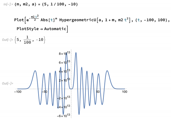
Next, let us prove sharp asymptotic estimates near infinity for the solutions of Equation (211).
Lemma 6.
Let be a non-trivial solution of Equation (211), where and λ are strictly positive and the exponent q satisfies (107). Then, for any , there exist and positive constants such that does not vanish in the interval and can be estimated by
Proof.
The proof is very similar to the proof in Theorem 5. The first part, that does not vanish in the interval if is large enough, is almost identical. Suppose there would exist a large such that
and let us also consider a real-valued . Then, multiplying Equation (211) by and integrating by parts over the interval would yield
a contradiction if is large enough.
Thus, let us assume that is strictly positive in the interval and let us consider the comparison function
where is an arbitrary constant. Then, satisfies in
The left-hand side of the preceding equation defines a differential operator and by an appropriate choice of and , we deduce
i.e., is a sub- resp. a super-solution depending on the choice of for the operator A if is large enough. Next, by making arbitrary but small, we define
and the constant such that
to obtain a sub-solution , and similarly, a super-solution is given by choosing
It is then fairly easy to infer
Indeed, to prove the second inequality, we multiply the inequality
in by and integrating by parts to deduce
which implies by the choice of . Hence, we conclude
The first inequality in (223) can be similarly derived, completing the proof of the lemma. □
Corollary 3.
The unitarily equivalent eigenfunctions can be estimated near infinity by
Proof.
This is obvious, since
□
4. Trace Class Estimates for
We consider the operator in (184) on page 19, which is essentially self-adjoint in
where
with
where q satisfies the relation (187) and we shall also use the same symbol for its closure, i.e., we shall assume that is self-adjoint in with eigenvectors and with eigenvalues satisfying the statements in Theorem 7 on page 18.
Let us also assume that all Hilbert spaces are complex vector spaces with a positive definite sesquilinear form (hermitian scalar product).
We shall now prove that
is of trace class in .
Theorem 9.
Let , then the operator
is of trace class in , i.e.,
The proof is essentially the proof given in [[5], Section 6] and [[3], Chapter 3.5] with the necessary modifications due to the different exponent in . A detailed proof for the general exponent q, , is given in [[11], Section 4].
Remark 4.
This result enables us to apply quantum statistics to our model of quantum gravity and to define a partition function Z, a density operator ρ and the von Neumann entropy S in a corresponding Fock space. For details, we refer the reader to [[3], Chapter 9.5].
5. Conclusions
In our model of quantum gravity, the physical states are described by solutions of a hyperbolic equation in a fiber bundle with base space , which is isometric to a Cauchy hypersurface of the quantized spacetime. The solutions of the hyperbolic equation can be expressed as a product of temporal and spatial eigenfunctions of self-adjoint operators acting in appropriate Hilbert spaces. The coefficients of the temporal eigenfunction equation as well as the corresponding eigenfunctions have a singularity in similar to the big bang singularity of the quantized spacetime.
However, by introducing a scalar field map
in the quantization process, we proved in Theorem 8 on page 21 that there exists a complete sequence of unitarily equivalent temporal eigenfunctions which solve the eigenfunction equation
in the interval , where and are strictly positive and
is a fixed exponent, such that the solutions can be evenly or oddly mirrored to the negative axis as sufficiently smooth functions across the singularity, provided the dimension k of the target space of is sufficiently large. Equation (236) is then valid in such that both sides smoothly vanish in . A plot before Lemma 6 on page 23 illustrates the situation. Moreover, we proved in Lemma 6 that the eigenfunctions vanish exponentially fast near infinity, which is also valid for the unitarily equivalent eigenfunctions , cf. Corollary 3 on page 24.
The hyperbolic equation in the fiber bundle comprised second-order differential operators acting in the fibers as well as in the base space. The temporal equation, which we consider here, also defines a second-order differential operator acting in the fibers because the Riemannian metrics, which are part of the variables after quantization, can be written in the form
where and the , , are elements of a subbundle with fibers such that by fixing an arbitrary metric which is supposed to be the induced metric of a Cauchy hypersurface of the quantized spacetime, we may assume, after choosing an appropriate atlas depending on , that each fiber is isometric to the symmetric space
cf. Section 1. The elementary gravitons are then eigenfunctions of the Laplacian in X. The corresponding eigenvalues are already incorporated in the coefficient of the temporal differential operator such that we are allowed to consider, besides the temporal operator, only spatial operators acting in .
Thus, we look at a quantum spacetime Q which can be written as a product
and at self-adjoint operators and acting in appropriate Hilbert spaces such that the remaining hyperbolic equation in Q can be expressed in the form
where u is a product of temporal and spatial eigenfunctions of resp.
cf. [3,5,6] for more details.
Since the temporal eigenfunctions can be smoothly mirrored to the negative axis, we may consider a second quantum spacetime
in which Equation (241) is also valid. Moreover, Equation (236) is even valid in across the singularity. Hence, we have to face the question of how to interpret this behavior. If we assume that has the same light cone as Q, then the singularity in lies in the future of , and since the mirrored eigenfunctions become unbounded if t tends to zero, the singularity in would be called a big crunch, i.e., would end in a big crunch but the corresponding classical spacetime would not start with a big bang in view of the results in Lemma 6 and Corollary 3 on page 24.
Hence, we have to assume that has the opposite time orientation, i.e., the singularity in is also a big bang for . In [6] and [[3], Chapter 5], we proved that we may consider to be a spatial self-adjoint operator defined by the fields of the Standard Model. If is invariant with respect to parity and charge conjugation, then in view of the CPT theorem, we would conclude that at the big bang, two universes were created with different time orientation, one filled with matter and the other with antimatter.
Funding
This research received no external funding.
Data Availability Statement
Data are contained within the article.
Acknowledgments
For the publication fee we acknowledge financial support by Heidelberg University.
Conflicts of Interest
The author declares no conflicts of interest.
References
- Gerhardt, C. The quantization of gravity in globally hyperbolic spacetimes. Adv. Theor. Math. Phys. 2013, 17, 1357–1391. [Google Scholar] [CrossRef] [Scilit]
- Arnowitt, R.; Deser, S.; Misner, C.W. The Dynamics of General Relativity; Witten, L., Ed.; Gravitation: An introduction to current research; John Wiley: New York, NY, USA, 1962; pp. 227–265. [Google Scholar]
- Gerhardt, C. The Quantization of Gravity, 2nd ed.; Fundamental Theories of Physics; Springer: Cham, Switzerland, 2024; Volume 194. [Google Scholar] [CrossRef] [Scilit]
- Gerhardt, C. The quantization of gravity: Quantization of the Hamilton equations. Universe 2021, 7, 91. [Google Scholar] [CrossRef] [Scilit]
- Gerhardt, C. The quantization of gravity: The quantization of the full Einstein equations. Symmetry 2023, 15, 1599. [Google Scholar] [CrossRef] [Scilit]
- Gerhardt, C. A unified quantization of gravity and other fundamental forces of nature. Universe 2022, 8, 404. [Google Scholar] [CrossRef] [Scilit]
- Olver, F.W.J.; Lozier, D.W.; Boisvert, R.F.; Clark, C.W. (Eds.) NIST Handbook of Mathematical Functions; Cambridge University Press: Cambridge, UK; New York, NY, USA; Melbourne, Australia, 2010. (In English) [Google Scholar]
- Kamke, E. Gewöhnliche Differentialgleichungen, 10th ed.; unchanged reprint of the 8th, revised edition; Teubner, S., Ed.; Teubner: Berlin, Germany, 1983. (In German) [Google Scholar]
- Courant, R.; Hilbert, D. Methoden der Mathematischen Physik. I; Dritte Auflage, Heidelberger Taschenbücher, Band 30; Springer: Berlin, Germany, 1968. [Google Scholar] [CrossRef] [Scilit]
- Maurin, K. Methods of Hilbert Spaces; Translated from the Polish by Andrzej Alexiewicz and Waclaw Zawadowski; Monografie Matematyczne; Państwowe Wydawnictwo Naukowe: Warsaw, Poland, 1967; Volume 45. [Google Scholar]
- Gerhardt, C. Extending the Solutions and the Equations of Quantum Gravity Past the Big Bang Singularity. arXiv 2025, arXiv:2501.13113. [Google Scholar] [CrossRef] [Scilit]
Disclaimer/Publisher’s Note: The statements, opinions and data contained in all publications are solely those of the individual author(s) and contributor(s) and not of MDPI and/or the editor(s). MDPI and/or the editor(s) disclaim responsibility for any injury to people or property resulting from any ideas, methods, instructions or products referred to in the content. |
© 2025 by the author. Licensee MDPI, Basel, Switzerland. This article is an open access article distributed under the terms and conditions of the Creative Commons Attribution (CC BY) license (https://creativecommons.org/licenses/by/4.0/).