Gauge Transformation Effects of Nonlocal Potentials in the Strong-Field Approximation for Complex Molecules

Abstract

In ultrafast science, the strong-field approximation (SFA) provides a powerful framework to describe high-order harmonic generation (HHG) and related phenomena. Meanwhile, within the current ab initio theoretical framework, the use of nonlocal potentials in calculating multi-electron molecular wave functions is almost unavoidable. We find that when such wave functions are directly applied to compute transition dipole moments for correcting SFA, it introduces a fundamental gauge transformation problem. Specifically, the nonlocal potential contributes an additional gauge-dependent phase function to the dipole operator, which directly modifies the phase of the transition dipole. As a consequence, the saddle-point equations acquire an entirely different structure compared to the standard SFA, leading to a splitting of the conventional short and long classical trajectories in HHG into multiple distinct quantum trajectories. Here, “complex molecules” refers to multi-center molecular systems whose nonlocal electronic structure leads to gauge-dependent strong-field responses. Our analysis highlights that the validity of gauge in-variation cannot be assumed universally in SFA framework. Our approach combines the molecular strong-field approximation with gauge transformation analysis, incorporating nonlocal pseudopotentials, saddle-point equations, and multi-center recombination effects.

1. Introduction

SFA theory has long served as a cornerstone in describing HHG and other strong-field processes in atoms and molecules [1,2,3,4,5]. Within this framework, the transition dipole moment between the continuum and bound states plays a central role, as it directly governs the ionization and recombination steps in HHG and the photoelectron spectra in high-order above-threshold ionization (HATI)s [6,7,8]. In its original formulation, the SFA relies on the assumption that the active electron can be approximated by a hydrogenic orbital or by a simple molecular orbital constructed from linear combinations of atomic orbitals (LCAO) [9,10]. Under these conditions, transition dipole moments are obtained from model wave functions derived from local potentials, and therefore no fundamental gauge-transformation issues arise (apart from the well-known R-dependent dipole ambiguity [11]). This explains why early SFA-based calculations could successfully reproduce many experimental features without encountering fundamental inconsistencies [12,13].

With the growing interest in complex molecular systems, however, the situation changes considerably. When hydrogen-like or LCAO-type wave functions are no longer sufficient for describing transition dipoles, a natural strategy is to employ ab initio quantum chemistry packages to compute molecular orbitals and thereby extract dipole matrix elements [14,15,16]. These program packages almost inevitably rely on nonlocal pseudopotentials or Hartree–Fock/Kohn–Sham orbitals in order to account for electron correlation and exchange effects [17,18], and has been widely adopted in calculations of ATI, HHG, molecular orbital tomography, and attosecond streaking reconstructions of single attosecond pulse and Wigner-type time delays [19,20,21].

However, since the introduction of nonlocal potentials, the associated issues of gauge transformation have been the subject of extensive discussion [22,23,24,25,26,27,28,29,30]. In recent years, with the application of time-dependent density functional theory (TDDFT) and Hartree–Fock (HF) theory to the nonlinear response of matter under strong laser fields, this problem has also attracted considerable attention in the ultrafast science community. For example, ref. [31] pointed out that, when solving the single-electron time-dependent Schrödinger equation, replacing the Coulomb potential with a nonlocal potential—an approach consistent with the use of more “accurate” dipole matrix elements in SFA calculations of HHG or ATI spectra—may lead to pronounced gauge dependence in the computed photoelectron spectra, and length gauge is a better choice.

In this work, we demonstrate that the use of dipole moment generated from nonlocal potentials introduces a fundamental gauge-transformation problem, closely analogous to the long-recognized issue in the semiconductor Bloch equations (SBE) for solids [32]. Strikingly, this complication has not been systematically identified in previous studies of molecular SFA model.

SFA is an approximation and cannot be gauge invariant. Our work does not attempt to enforce gauge invariance of SFA, but rather quantifies the gauge-dependent phase errors introduced by nonlocal potentials in molecular strong-field dynamics. The essence of this gauge transformation problem lies in the fact that, when using a Hamiltonian with a nonlocal potential, the position operator no longer commutes with the binding potential. To ensure gauge invariance within the SFA framework, it is necessary to apply a gauge correction to the dipole. Specifically, an additional phase must be introduced in the Volkov action of the SFA equations, whether formulated in the length or velocity gauge.

This gauge correction changes the saddle-point equations that determine the electron quantum orbits [33,34]. Consequently, the corresponding saddle-point equations no longer yield only four sets of symmetric solutions, but may instead produce additional asymmetric solutions. Although the additional dipole phase arising from the gauge transformation issue can be attributed to numerical artifacts, we also endeavor to interpret this correction within a physical framework (at least for some cases): the use of an appropriate nonlocal potential enables a more accurate treatment of electron–electron and electron–nuclear interactions in complex molecular systems. In the presence of a strong laser field, nonlocal potentials naturally incorporate scattering and correlation effects that are largely suppressed in local single-electron approximations. As a consequence, the electronic wave packet becomes more prone to quantum diffraction, leading to the splitting of classical trajectories into multiple quantum paths. This, in turn, causes the corresponding saddle-point equations to yield not only the conventional four symmetric solutions, but also additional asymmetric ones.

Recognizing this nonlocal-potential-induced gauge problem carries both theoretical and practical implications. Theoretically, it delineates the limitations of applying standard SFA-based models to complex molecular systems. Computationally, it highlights the necessity of carefully treating the dipole operator in pseudopotential-based simulations to ensure gauge-consistent results. In this paper, we provide a systematic analysis of the gauge-transformation problem induced by nonlocal potentials within the SFA framework.

We begin our discussion with the mathematical derivation of gauge transformations induced by nonlocal potentials. Unless otherwise specified, atomic units are used throughout this work.

2. Gauge Transformation Problem from Nonlocal Potentials

The field-free single-electron Hamiltonian is written as

$${\widehat{H}}_0={\displaystyle \frac{{\widehat{\mathbf{p}}}^2}{2}}+\widehat{V},$$

(1)

where $\widehat{V}$ is the binding potential (which may be local or nonlocal). If $\widehat{V}$ is a local multiplicative potential, $V\left(\mathbf{r}\right)$, then $[\widehat{V},\widehat{\mathbf{r}}]=\mathbf{0}$ and one obtains the familiar commutator identity

$$[{\widehat{H}}_0,\widehat{\mathbf{r}}]=\left[\frac{{\widehat{\mathbf{p}}}^2}{2},\widehat{\mathbf{r}}\right]=-i\widehat{\mathbf{p}},$$

(2)

or equivalently

$$\widehat{\mathbf{p}}=i[{\widehat{H}}_0,\widehat{\mathbf{r}}].$$

(3)

Let $\left\{\right|n⟩\}$ be eigenstates of ${\widehat{H}}_0$ with eigenvalues $E_n$:

$${\widehat{H}}_0|n⟩=E_n|n⟩.$$

For $n\ne m$, the matrix element of $\widehat{\mathbf{p}}$ follows immediately:

$$\begin{array}{cc}\hfill ⟨n\left|\widehat{\mathbf{p}}\right|m⟩& =i⟨n\left|[{\widehat{H}}_0,\widehat{\mathbf{r}}]\right|m⟩\hfill \end{array}$$

(4)

$$\begin{array}{cc}\hfill & \hspace{1em}\hspace{1em}\hspace{1em}\hspace{1em}\hspace{0.17em} =i(E_n-E_m)⟨n|\widehat{\mathbf{r}}|m⟩\hfill \end{array}$$

(5)

$$\begin{array}{cc}\hfill & \hspace{1em}\hspace{1em}\hspace{0.17em}\equiv i{\omega }_{nm}⟨n|\widehat{\mathbf{r}}|m⟩,\hfill \end{array}$$

(6)

where n, m label the two molecular orbitals involved in the transition matrix element and we define ${\omega }_{nm}\equiv E_n-E_m$. The factor i implies a $\pi /2$ relative phase between momentum- and position-space matrix elements.This is the basis for the usual equivalence of length- and velocity-gauge dipoles when the potential is local.

If $\widehat{V}$ is nonlocal, it acts via a kernel

$$\left(\widehat{V}\psi \right)\left(\mathbf{r}\right)=\int d^3{r}^{\prime }V(\mathbf{r},{\mathbf{r}}^{\prime })\psi \left({\mathbf{r}}^{\prime }\right).$$

(7)

In this case the commutator with $\widehat{\mathbf{r}}$ is generally nonzero. Defining the operator

$$\widehat{\mathrm{\Delta }}\equiv [\widehat{V},\widehat{\mathbf{r}}],$$

(8)

its action on a test function is

$$\left(\widehat{\mathrm{\Delta }}\psi \right)\left(\mathbf{r}\right)=\int d^3{r}^{\prime }V(\mathbf{r},{\mathbf{r}}^{\prime })({\mathbf{r}}^{\prime }-\mathbf{r})\psi \left({\mathbf{r}}^{\prime }\right).$$

(9)

The length-gauge transform of the nonlocal operator $\widehat{V}$ is

$${\widehat{V}}_L\left(t\right)=U_{\mathrm{GM}}\left(t\right)\widehat{V}{U}_{\mathrm{GM}}^{†}\left(t\right).$$

where $U_{GM}$ is the Göppert–Mayer unitary and $\mathbf{A}$ is the laser vector potential, satisfying $\mathbf{E}\left(t\right)=-{\partial }_t\mathbf{A}\left(t\right)$.

$$U_{\mathrm{GM}}\left(t\right)=e^{i\widehat{\mathbf{r}}·\mathbf{A}\left(t\right)}.$$

Using the Baker–Campbell–Hausdorff (BCH) operator expansion,

$$\begin{array}{c}{\widehat{V}}_L\left(t\right)=e^{i\widehat{\mathbf{r}}·\mathbf{A}}\widehat{V}{e}^{-i\widehat{\mathbf{r}}·\mathbf{A}}\hfill \\ =\widehat{V}+i[\widehat{\mathbf{r}}·\mathbf{A},\widehat{V}]+\frac{i^2}{2!}[\widehat{\mathbf{r}}·\mathbf{A},[\widehat{\mathbf{r}}·\mathbf{A},\widehat{V}]]+\cdots .\hfill \end{array}$$

Since $\mathbf{A}$ is a c-number vector (classical field), it factors out of commutators. Using

$$[\widehat{\mathbf{r}}·\mathbf{A},\widehat{V}]=-\mathbf{A}·[\widehat{V},\widehat{\mathbf{r}}]=-\mathbf{A}·\widehat{\mathrm{\Delta }},$$

we obtain to first order

$${\widehat{V}}_L\left(t\right)=\widehat{V}-i\mathbf{A}\left(t\right)·\widehat{\mathrm{\Delta }}+\mathcal{O}\left(A^2\right),$$

(10)

higher-order terms $\mathcal{O}\left(A^2\right)$ involve nested commutators (equivalently, moments like $\int {(\mathbf{r}-{\mathbf{r}}^{\prime })}^{\otimes 2}V(\mathbf{r},{\mathbf{r}}^{\prime })\psi \left({\mathbf{r}}^{\prime }\right)$) and may become relevant for very strong fields or very long-range kernels. Nevertheless, such terms mainly enhance the degree of gauge co-variance and do not alter the conclusions of our mathematical derivation. Therefore the full commutator becomes

$$[{\widehat{H}}_0,\widehat{\mathbf{r}}]=-i\widehat{\mathbf{p}}+\widehat{\mathrm{\Delta }},$$

(11)

and the canonical relation (3) is replaced by

$$\widehat{\mathbf{p}}=i[{\widehat{H}}_0,\widehat{\mathbf{r}}]-i\widehat{\mathrm{\Delta }}.$$

(12)

Then for a transition between states $|m⟩$ and $|n⟩$, Equation (12) gives

$$\begin{array}{cc}\hfill ⟨m\left|\widehat{\mathbf{p}}\right|n⟩& =i⟨m|[{\widehat{H}}_0,\widehat{\mathbf{r}}]|n⟩-i⟨m|\widehat{\mathrm{\Delta }}|n⟩\hfill \\ \hfill & =i(E_m-E_n)⟨m|\widehat{\mathbf{r}}|n⟩-i⟨m|\widehat{\mathrm{\Delta }}|n⟩.\hfill \end{array}$$

(13)

In SFA applications, one often considers a continuum state $|\mathbf{q}⟩$ (asymptotic momentum label) and the ground state $|0⟩$. Defining the usual length-gauge transition dipole

$$\mathbf{d}\left(\mathbf{q}\right)\equiv ⟨\mathbf{q}\left|\widehat{\mathbf{r}}\right|0⟩,$$

(14)

and the continuum–bound energy difference ${\omega }_{\mathbf{q}0}\equiv E_{\mathbf{q}}-E_0$, we introduce the nonlocal correction vector

$$\mathbf{C}\left(\mathbf{q}\right)\equiv ⟨\mathbf{q}\left|\widehat{\mathrm{\Delta }}\right|0⟩.$$

(15)

Equation (13) then yields the corrected velocity (momentum) matrix element

$$\mathbf{v}\left(\mathbf{q}\right)\equiv ⟨\mathbf{q}|\widehat{\mathbf{p}}|0⟩=i{\omega }_{\mathbf{q}0}\mathbf{d}\left(\mathbf{q}\right)-i\mathbf{C}\left(\mathbf{q}\right).$$

(16)

Thus, for nonlocal $\widehat{V}$, the simple proportionality between $\mathbf{v}\left(\mathbf{q}\right)$ (dipole with velocity gauge) and $\mathbf{d}\left(\mathbf{q}\right)$ (dipole with length gauge) is broken by the additive term $\mathbf{C}\left(\mathbf{q}\right)$, which generally has both real and imaginary parts and therefore changes both amplitude and phase of the transition matrix element. This gauge co-variation degree can be estimated by a convenient dimensionless diagnostic:

$$R\left(\mathbf{q}\right)\equiv {\displaystyle \frac{\left|C\right(\mathbf{q}\left)\right|}{{\omega }_{\mathbf{q}0}\left|d\left(\mathbf{q}\right)\right|}},$$

(17)

Next, we analyze mathematically and numerically which types of nonlocal potentials most strongly affect the gauge invariance of dipole matrix elements in the SFA. The dimensionless parameter $R\left(\mathbf{q}\right)$ is employed to quantify the relative strength of gauge-dependent corrections.

A simple upper bound can be written in terms of the first moment of the kernel:

$$\parallel \widehat{\mathrm{\Delta }}\parallel \le \underset{\mathbf{r}}{sup}\int d^3{r}^{\prime }|V_{\mathrm{nl}}(\mathbf{r},{\mathbf{r}}^{\prime })\left|\right|{\mathbf{r}}^{\prime }-\mathbf{r}|\equiv {\mathcal{M}}_1\left[V_{\mathrm{nl}}\right],$$

(18)

so that the gauge effect grows with the kernel’s range and magnitude.

• Coordinate space.

If the nonlocal kernel has support of size L and strength $V_0$, then

$$\parallel \widehat{\mathrm{\Delta }}\parallel \sim \mathcal{O}\left(V_{0}L\right),$$

(19)

indicating that wide or strong kernels amplify gauge sensitivity.

b.

Momentum space.

In momentum representation,

$$⟨\mathbf{k}|\widehat{\mathrm{\Delta }}|{\varphi }_0⟩=i\int {\displaystyle \frac{d^3{k}^{\prime }}{{\left(2\pi \right)}^3}}{\displaystyle \frac{\partial }{\partial \mathbf{k}}}{V}_{\mathrm{nl}}(\mathbf{k},{\mathbf{k}}^{\prime }){\tilde{\varphi }}_0\left({\mathbf{k}}^{\prime }\right).$$

(20)

Sharp momentum gradients (e.g., from hard-core projectors or high angular momentum channels) enhance $\widehat{\mathrm{\Delta }}$.

We consider three commonly used types of nonlocal potentials in molecular SFA calculations and analyze their impact on gauge invariance:

1. Pseudopotential projectors. These are widely used to reduce the number of electrons explicitly treated [35,36]. The nonlocal operator is typically written as

$${\widehat{V}}_{\mathrm{nl}}=\sum _{l,m}|{\beta }_{lm}⟩v_l⟨{\beta }_{lm}|,$$

(21)

where ${\beta }_{lm}\left(\mathbf{r}\right)$ is a localized projector function, and $v_l$ is the channel potential. The commutator with the position operator is

$$\widehat{\mathrm{\Delta }}=[{\widehat{V}}_{\mathrm{nl}},\widehat{\mathbf{r}}]=\sum _{l,m}|{\beta }_{lm}⟩v_l⟨{\beta }_{lm}|(\widehat{\mathbf{r}}-{\mathbf{R}}_c),$$

(22)

where ${\mathbf{R}}_c$ is the center of the projector. The dipole correction is

$$⟨\mathbf{q}|\widehat{\mathrm{\Delta }}|{\varphi }_0⟩=\sum _{l,m}{v}_l{\Phi }_{lm}\left(\mathbf{q}\right)\left(⟨{\beta }_{lm}|\widehat{\mathbf{r}}|{\varphi }_0⟩-{\mathbf{R}}_c⟨{\beta }_{lm}|{\varphi }_0⟩\right),$$

(23)

with ${\Phi }_{lm}\left(\mathbf{q}\right)=\int d^{3}r{\beta }_{lm}\left(\mathbf{r}\right)e^{-i\mathbf{q}·\mathbf{r}}$. Therefore, the correction is amplified for large projector radii $r_c$, strong channel potentials $v_l$, and high angular momentum channels (l > 0), especially when ${\varphi }_0$ has significant amplitude within the projector support.

2. Separable rank-1 kernels. These are simple model nonlocal potentials [37], often used for analytical insight:

$$V_{\mathrm{nl}}(\mathbf{r},{\mathbf{r}}^{\prime })=V_0\phi \left(\mathbf{r}\right){\phi }^{*}\left({\mathbf{r}}^{\prime }\right).$$

(24)

The commutator gives

$$⟨\mathbf{q}|\widehat{\mathrm{\Delta }}|{\varphi }_0⟩=V_0\left[{\Phi }^{*}\left(\mathbf{q}\right)⟨\phi |\widehat{\mathbf{r}}|{\varphi }_0⟩-{\widetilde{\left(\mathbf{r}\phi \right)}}^{*}\left(\mathbf{q}\right)⟨\phi |{\varphi }_0⟩\right],$$

(25)

where $\Phi \left(\mathbf{q}\right)$ and $\widetilde{\left(\mathbf{r}\phi \right)}\left(\mathbf{q}\right)$ are Fourier transforms of $\phi$ and $\mathbf{r}\phi$, respectively. Thus, the effect on the dipole phase is controlled by the width of $\phi$, the amplitude $V_0$, and the overlap with ${\varphi }_0$. Narrow, strongly overlapping projectors lead to larger R values.

3. Exchange operators in Hartree–Fock and hybrid DFT. The Fock operator introduces intrinsic nonlocality due to exchange [38,39]:

$$\left(\widehat{K}\psi \right)\left(\mathbf{r}\right)=\sum _j{\varphi }_j\left(\mathbf{r}\right)\int d^3{r}^{\prime }{\displaystyle \frac{{\varphi }_j^{*}\left({\mathbf{r}}^{\prime }\right)\psi \left({\mathbf{r}}^{\prime }\right)}{|\mathbf{r}-{\mathbf{r}}^{\prime }|}}.$$

(26)

The commutator $\widehat{\mathrm{\Delta }}=[\widehat{K},\widehat{\mathbf{r}}]$ can be approximated by

$$\parallel \widehat{\mathrm{\Delta }}\parallel \sim {\alpha }_{\mathrm{x}}\xi ,$$

(27)

where ${\alpha }_{\mathrm{x}}$ is the fraction of exact exchange and $\xi$ is the characteristic decay length of the exchange kernel. In molecules with highly delocalized orbitals or multiple centers, $\xi$ can be large, moderately increasing R. However, symmetry and orbital orthogonality usually suppress the effective contribution to the dipole phase.

To assess the impact of nonlocal potentials on dipole phase gauge invariance, we perform a rough numerical estimation using representative molecular parameters of the dimensionless ratio Equation (17). Here the typical parameter ranges: Electron momentum: $\left|\mathbf{q}\right|\sim 0.5$–$1.5$ a.u., ionization potential: $I_p\sim 0.4$–1 a.u., the dipole magnitude: $\left|\mathbf{d}\right(\mathbf{q}\left)\right|\sim 0.1$–1 a.u.. Therefore, estimated $R\left(\mathbf{q}\right)$ values for pseudopotential projectors (large $r_c$, strong $v_l$) have $R\sim 0.7$–$2.0$, Separable Gaussian kernels (moderate width and overlap) have $R\sim 0.2$–$0.8$ and Fock exchange (hybrid DFT, delocalized orbitals) have $R\sim 0.05$–$0.3$.

Using these representative values, we find that different families of nonlocal potentials lead to distinct characteristic ranges of $R\left(\mathbf{q}\right)$. Pseudopotential projectors (large $r_c$ and strong $v_l$) typically give $R\sim 0.7$–$2.0$, reflecting their strong short-range nonlocality. Separable Gaussian kernels with moderate width and orbital overlap give intermediate values $R\sim 0.2$–$0.8$. Fock-exchange-type nonlocality appearing in hybrid DFT and delocalized molecular orbitals results in weaker nonlocal corrections, with $R\sim 0.05$–$0.3$. These quantitative estimates illustrate that gauge-dependent dipole-phase corrections are most significant in systems with strongly localized nonlocal potentials, but can remain non-negligible even for delocalized molecular orbitals.

From above analysis, we can summary that pseudopotential projectors with large $r_c$, strong $v_l$, and high l channels may have strongest effect, separable rank-1 kernels with significant overlap and moderate width take the medium position, and Fock exchange in hybrid DFT, enhanced for delocalized molecules has moderate effect.

It should be emphasized that the above analysis is rather approximate and qualitative. Depending on the choice of pseudopotentials and exchange–correlation functionals employed in different quantum chemistry packages, the resulting numerical values may vary considerably. For clarity, we provide in the Supplementary Materials a detailed numerical scheme for estimating $R\left(q\right)$.

Here we classify molecules according to their expected sensitivity. Molecules expected to show significant gauge-dependent dipole phase corrections generally have one or more of the following characteristics:

1. Heavy atoms or multi-center systems: Examples include halogenated organics (e.g., containing I or Br). Heavy atoms often require strong pseudopotentials with large projector ranges and high angular momentum channels, resulting in a large commutator $[{\widehat{V}}_{\mathrm{nl}},\widehat{\mathbf{r}}]$ and substantial modification of the dipole phase.

2. High angular momentum orbitals: Molecules containing S, P, or transition metal centers. Projectors for higher angular momentum channels introduce stronger momentum-space gradients, enhancing $R\left(\mathbf{q}\right)$.

3. Highly delocalized molecular orbitals: Examples include conjugated systems, aromatic molecules, fullerenes, and metal complexes. Extended wavefunctions overlap multiple atomic centers, increasing the cumulative $\widehat{\mathrm{\Delta }}$ effect.

4. Hybrid DFT or systems with exchange contributions: Systems with a high fraction of exact exchange (${\alpha }_x$) and extended orbitals exhibit larger Fock nonlocal operator contributions, increasing $R\left(\mathbf{q}\right)$.

Molecules with minimal gauge-dependent dipole corrections typically exhibit:

1. Small, light-atom molecules: H₂, HeH⁺, H₂O, CO₂, etc. Nonlocal potentials are weak and wavefunctions are localized, leading to $R\left(\mathbf{q}\right)\ll 0.1$.

2. Localized orbitals: Saturated alkanes or molecules dominated by localized $\sigma$ bonds. The dipole phase correction from nonlocal operators is minimal.

3. Light-element systems without strong pseudopotentials or exchange operators: Pure hydrides or oxides treated with low-level HF or Local Density Approximation (LDA)/semilocal DFT. Nonlocality is small and gauge-related dipole phase corrections are negligible.

Nonlocal pseudopotentials are widely used in molecular and condensed-matter simulations, yet their behavior under gauge transformations remains subtle. In this subsection, we present a self-contained and gauge-theoretically consistent formulation of nonlocal potentials, independent of any strong-field approximation:

1. Peierls/Schwinger Phase Factor for Nonlocal Operators

A general nonlocal potential takes the form

$${\widehat{V}}_{\mathrm{nl}}\psi \left(\mathbf{r}\right)=\int d{\mathbf{r}}^{\prime }{V}_{\mathrm{nl}}(\mathbf{r},{\mathbf{r}}^{\prime })\psi \left({\mathbf{r}}^{\prime }\right).$$

(28)

Under a gauge transformation generated by a scalar function $\chi (\mathbf{r},t)$,

$$\psi \to e^{i\chi }\psi ,\mathbf{A}\to \mathbf{A}+\nabla \chi ,$$

(29)

gauge covariance requires the nonlocal operator itself to transform as

$$V_{\mathrm{nl}}(\mathbf{r},{\mathbf{r}}^{\prime })\to V_{\mathrm{nl}}(\mathbf{r},{\mathbf{r}}^{\prime })exp\left[i{\int }_{{\mathbf{r}}^{\prime }}^{\mathbf{r}}\mathbf{A}·d\ell \right].$$

(30)

This exponential factor is known as the Peierls or Schwinger nonlocal phase factor [40,41,42]. Physically, it represents the Wilson-line phase accumulated by a virtual electron displaced between two centers [43,44,45,46]. Only with Equation (30) is the Hamiltonian gauge-covariant.

2. Why Standard Pseudopotentials Break Gauge Covariance

Most norm-conserving and separable pseudopotentials (e.g., Kleinman–Bylander forms) are constructed without the Wilson-line phase. As a result, under a gauge transformation the Hamiltonian does not obey the required covariance relation, and physical observables may develop unphysical gauge dependence—especially in strong-field and time-dependent scenarios where $\mathbf{A}\left(t\right)$ is large.

This breakdown is particularly severe for

• Multi-center molecular systems;
• Large internuclear separations;
• Heavy atoms with strongly nonlocal pseudopotentials.

3. First-Order Working Approximation Used in This Paper

To implement the correct phase factor in practical strong-field calculations, we adopt the controlled first-order expansion:

$$exp\left[i{\int }_{{\mathbf{r}}^{\prime }}^{\mathbf{r}}\mathbf{A}\left(t\right)·d\ell \right]\approx 1+i\mathbf{A}\left(t\right)·(\mathbf{r}-{\mathbf{r}}^{\prime })+\mathcal{O}\left(A^2\right),$$

(31)

which is justified for the following reasons:

(a)

The field is spatially homogeneous (dipole approximation);

(b)

Higher-order terms contribute only weak corrections to HHG phase in the intensities considered here;

(c)

The linear term already captures the leading nonlocal gauge-induced phase, which is the main focus of this work.

The resulting Hamiltonian is used as input for all strong-field amplitude calculations in the following sections.

3. Numerical Verification and Discussions

As an illustrative case, we consider HHG to clarify our mathematical analysis. The standard SFA HHG amplitude in the length gauge is [1,11,47]:

$$\mathcal{A}\propto \int dt{\int }^{t}d{t}^{\prime }\int d^{3}k{\mathbf{d}}^{*}\left({\mathbf{q}}_t\right)\mathbf{E}\left(t^{\prime }\right)·\mathbf{d}\left({\mathbf{q}}_{t^{\prime }}\right)e^{-iS(\mathbf{k},t,t^{\prime })},$$

(32)

where $\mathbf{d}$ is the momentum space transition dipole moment. $\mathbf{E}$ is the electric field, denoted as a plane wave $E_{0}sin\left(\omega t\right)$ throughout this work, ${\mathbf{q}}_{\tau }=\mathbf{k}+\mathbf{A}\left(\tau \right)$ with $\mathbf{A}$ is the vector potential of $\mathbf{E}$ and $S(\mathbf{k},t,t^{\prime })={\int }_{t^{\prime }}^{t}d\tau \frac{{\mathbf{q}}_{\tau }^2}{2}+I_p(t-t^{\prime })$ is the Volkov action. $I_p$, t and $t^{\prime }$ correspond with the potential energy, photon emission time, and ionization time, respectively.

Additionally, the Volkov propagator describes the continuum electron in the presence of a classical laser field and corresponds to the exact solution of the time-dependent Schrödinger equation for a free electron coupled to an electromagnetic vector potential. Physically, a Volkov state can be viewed as a plane wave “dressed” by the laser: the electron undergoes quiver motion driven by the field and accumulates a semiclassical action ${\mathbf{S}}_{\mathrm{V}}(\mathbf{k},t,t^{\prime })={\int }_{t^{\prime }}^t{\displaystyle \frac{{[\mathbf{k}+\mathbf{A}\left(\tau \right)]}^2}{2}}d\tau .$ In the SFA, the Volkov propagator is used to model the electron’s continuum propagation between ionization and recombination while neglecting the binding potential except at the endpoints (ionization/recombination). This propagation produces the large, rapidly varying phase factors that dominate the saddle-point integration and determine the classical-like trajectories of returning electrons.

By analogy with the treatment of gauge transformation in the solid-state SBE theory [48,49,50], the dipole matrix elements must be corrected under nonlocal potentials in order to ensure the gauge invariance of the SFA equations. Write the dipole with a rephasing factor and an additive nonlocal correction:

$$\mathbf{d}\left(\mathbf{q}\right)\mapsto e^{i\chi \left(\mathbf{q}\right)}\overline{\mathbf{d}}\left(\mathbf{q}\right)+\delta {\mathbf{d}}_{\mathrm{\Delta }}\left(\mathbf{q}\right),$$

where $\delta {\mathbf{d}}_{\mathrm{\Delta }}$ denotes the additive correction induced by $\widehat{\mathrm{\Delta }}=[{\widehat{V}}_{\mathrm{nl}},\widehat{\mathbf{r}}]$. Substituting into Equation (32) gives

$$\mathcal{A}\propto \int dt{\int }^{t}d{t}^{\prime }\int d^{3}k\left[e^{-i\chi \left({\mathbf{q}}_t\right)}{\overline{\mathbf{d}}}^{*}\left({\mathbf{q}}_t\right)+\delta {\mathbf{d}}_{\mathrm{\Delta }}^{*}\left({\mathbf{q}}_t\right)\right]\mathbf{E}\left(t^{\prime }\right)·\left[e^{+i\chi \left({\mathbf{q}}_{t^{\prime }}\right)}\overline{\mathbf{d}}\left({\mathbf{q}}_{t^{\prime }}\right)+\delta {\mathbf{d}}_{\mathrm{\Delta }}\left({\mathbf{q}}_{t^{\prime }}\right)\right]e^{-iS}.$$

(33)

The induced dipole integral in the SFA contains a rapidly oscillating phase factor, and the saddle-point method can accurately capture the dominant contribution of this type of highly oscillatory integral [3]. The saddle-point solution $t_s^{\prime }$ identifies the complex ionization time when tunnel ionization occurs; the real parts of the saddle-point solution $t_s$ correspond to recollision times, and this time determines the quantum trajectory responsible for HHG.

We consider the HHG from the Ar $3p$ orbital and from the HOMO-2 orbital of the I₂ molecule, and examine the gauge sensitivity of different atomic and molecular systems. Before presenting the numerical results, we clarify why the I₂ molecule is chosen as our representative test system. In this work, we use the term “complex molecules” to refer to multi-center molecular systems whose electronic structure exhibits strong nonlocality, significant orbital delocalization, and substantial gauge-dependent phase contributions within the strong-field approximation. According to this definition, I₂ naturally falls into the category of complex molecules. Its large internuclear distance and multi-center electronic structure produce pronounced interference patterns in the recombination dipole, and its nonlocal potential components are considerably stronger than in lighter or more compact diatomic molecules. Furthermore, I₂ has been widely studied in the strong-field literature, making it a well-characterized benchmark for testing gauge-dependent effects in molecular HHG. For these reasons, I₂ serves as an ideal system for assessing the influence of nonlocal potentials on the dipole-phase gauge invariance in our work.

In the length gauge, the dipole is evaluated using Equation (14), while in the velocity gauge, the dipole is obtained from Equation (16). The gauge-corrected HHG in the length gauge is computed using Equation (33). The wavefunctions under the nonlocal potential, as well as the corresponding transition dipole moments between the initial and continuum states, are calculated with the quantum chemistry package octopus [51,52,53]. Details of the computational setup, parameters, and how to calculate the gauge-corrected terms are provided in the Supplementary Materials.

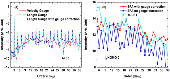
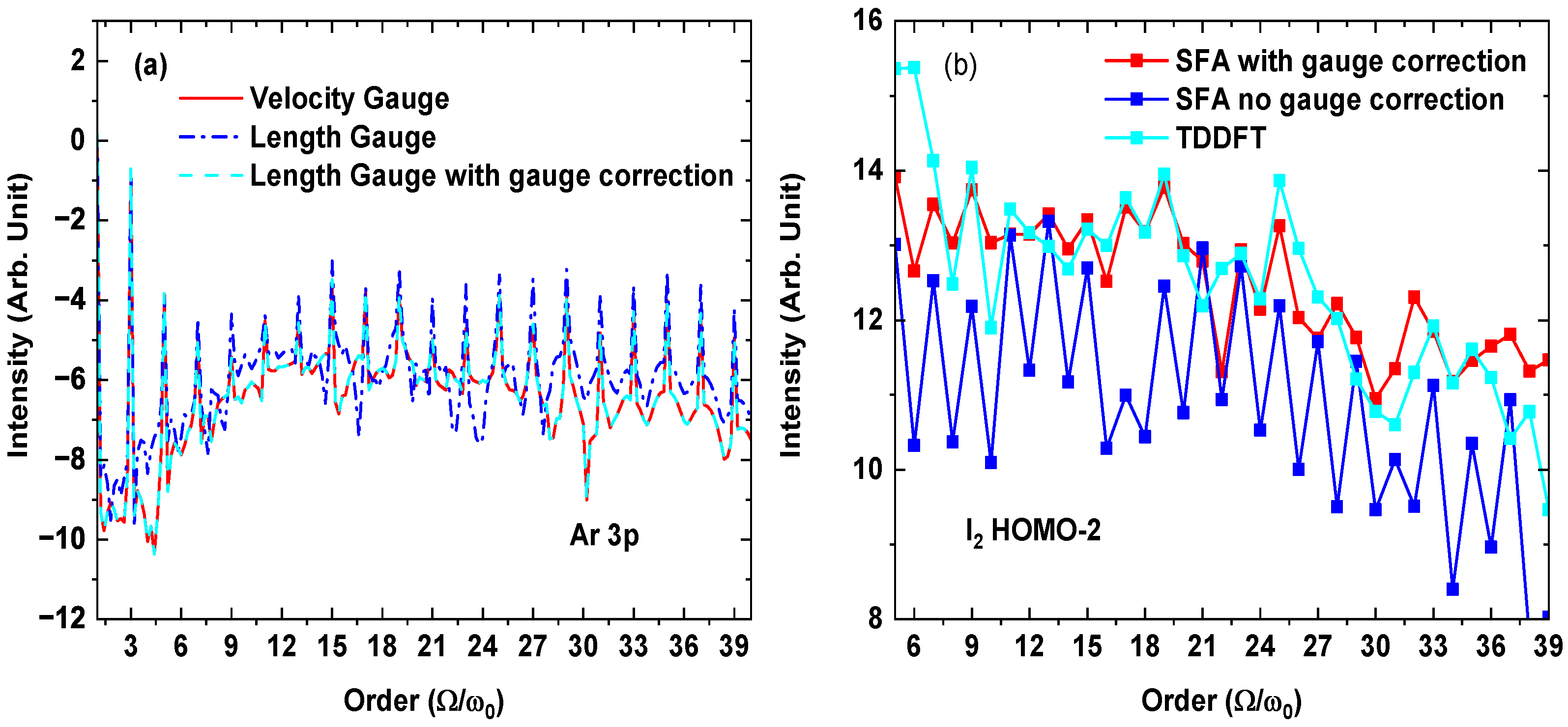
Figure 1a presents the HHG spectra of the Ar $3p$ orbital under three scenarios: the velocity gauge (red solid line), the length gauge (blue dashed line), and the gauge-corrected length gauge (cyan dashed line). As anticipated in the previous subsection, for a light atom such as Ar the influence of nonlocal potentials on the gauge transformation is negligible. After applying the gauge correction, the HHG spectra obtained from the length and velocity gauges are in excellent agreement.

Figure 1. (a) presents the HHG spectra of the Ar 3p orbital in the velocity gauge (red solid line), the length gauge (blue dashed line), and the gauge-corrected length gauge (cyan dashed line). (b) shows the HHG spectra of the HOMO-2 orbital of the I2 molecule in the gauge-corrected length gauge (equivalent to the velocity gauge, red line), the uncorrected length gauge (blue line) and the TDDFT in the octopus (cyan line).

In contrast, Figure 1b shows the HHG from the HOMO-2 orbital of the I₂ molecule. Here, the red line corresponds to the gauge-corrected length-gauge result (identical to the velocity-gauge spectrum, which is omitted for clarity), the blue line represents the uncorrected length-gauge spectrum. We observe that for I₂, which contains heavy iodine nuclei, the HHG intensity from gauge-corrected case is much stronger than the uncorrected one. Moreover, the peak-valley structure from uncorrected one is more pronounced. This results show that the impact of nonlocal potentials on the gauge transformation is considerably more pronounced for I₂.

Our numerical simulations are in good agreement with the predictions of our analytical model. For relatively simple atomic and molecular systems such as Ar, the effect of gauge covariance remains weak. In contrast, for heavier and more complex molecular systems such as iodine, the impact of gauge covariance becomes significant and cannot be neglected.

Consequently, the gauge-dependent correction arises fundamentally because a nonlocal binding operator ${\widehat{V}}_{\mathrm{nl}}$ does not commute with the position operator, i.e., $[{\widehat{V}}_{\mathrm{nl}},\widehat{\mathbf{r}}]\ne 0$. This non-commutation introduces an operator $\widehat{\mathrm{\Delta }}$, which contributes an additive term $\mathbf{C}\left(\mathbf{q}\right)=⟨\mathbf{q}\left|\widehat{\mathrm{\Delta }}\right|0⟩$ to the velocity matrix element. The vector $\mathbf{C}\left(\mathbf{q}\right)$ is, in general, complex and momentum-dependent; its phase modifies the effective phase of the recombination dipole.

Semiclassically, this correction can be interpreted as the extra phase accumulated when the released electron samples spatially separated parts of a multi-center potential during continuum propagation (e.g., ionizing at one atomic center and recombining at another). For such a process, an additional contribution of the form $\mathbf{k}·\mathrm{\Delta }\mathbf{R}$ to the recombination phase arises, where $\mathrm{\Delta }\mathbf{R}$ is the vector separation between ionization and recombination centers and $\mathbf{k}$ is the canonical momentum at recollision. This geometric/dynamical phase is negligible in single-center atoms but can be large in extended or heavy multi-center molecules, thereby producing observable gauge-dependent signatures in HHG.

Another central question is whether our modification to the SFA (especially the introduction of an additional phase) should be regarded merely as a mathematical artifact, or whether it carries genuine physical significance? To address this, in Figure 1b, we compare the gauge-corrected SFA with octopus TDDFT results for HHG (The cyan line in b panel). Our findings reveal that, except in the low-energy region, the length-gauge SFA with gauge correction agrees well with TDDFT. This agreement indicates that our gauge correction, at least for I₂ or similar molecules, to the SFA formula is not merely a numerical adjustment, but also reflects meaningful physical content.

However, whether this gauge correction carries physical significance for all elements and all types of nonlocal potentials still requires case-by-case analysis. In particular, one should compare the results after gauge correction with reliable reference calculations (such as TDDFT). In the following, we provide an analysis of the possible changes in physical interpretation induced by this gauge correction.

For the sake of clarity in the subsequent analysis, we define the additional phase introduced by the gauge correction in the length gauge as

$$\chi \left(\mathbf{q}\right)=-a{(\mathbf{q}-1)}^2{(\mathbf{q}+1)}^2,$$

(34)

where the coefficient a determines the curvature of the phase. The reason we employ this particular phase is that the HHG spectra calculated with it more readily reproduce the gauge-induced modifications observed in iodine molecules.

It is important to note that Equation (34) is not obtained by expanding the nonlocal potential or by performing a saddle-point approximation. Instead, $\chi \left(\mathbf{q}\right)=-a{(\mathbf{q}-1)}^2{(\mathbf{q}+1)}^2,a=3,$ is introduced as a model gauge-dependent phase that mimics the strongly momentum-dependent phase modulation found in heavy diatomic molecules such as ${\mathrm{I}}_2$. For such molecules, the nonlocal pseudopotential produces a highly structured gauge-induced phase that depends sensitively on the electron momentum. Direct analytic forms for this phase are generally not available. Therefore, we adopt the phenomenological form in Equation (34) to capture the essential features of the molecular phase while allowing us to systematically investigate the effect of gauge transformations within an analytically tractable setting. The chosen parameters reproduce the typical magnitude and qualitative shape of the momentum-dependent phase observed in numerical simulations of ${\mathrm{I}}_2$.

We emphasize that the conclusions of this work do not depend on the specific polynomial form of $\chi \left(\mathbf{q}\right)$; any sharply varying momentum-dependent phase typical of nonlocal heavy-molecule pseudopotentials would lead to the same qualitative gauge behavior. Equation (34) thus serves as a representative model to illustrate the underlying physics.

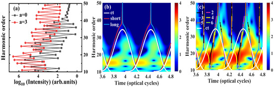
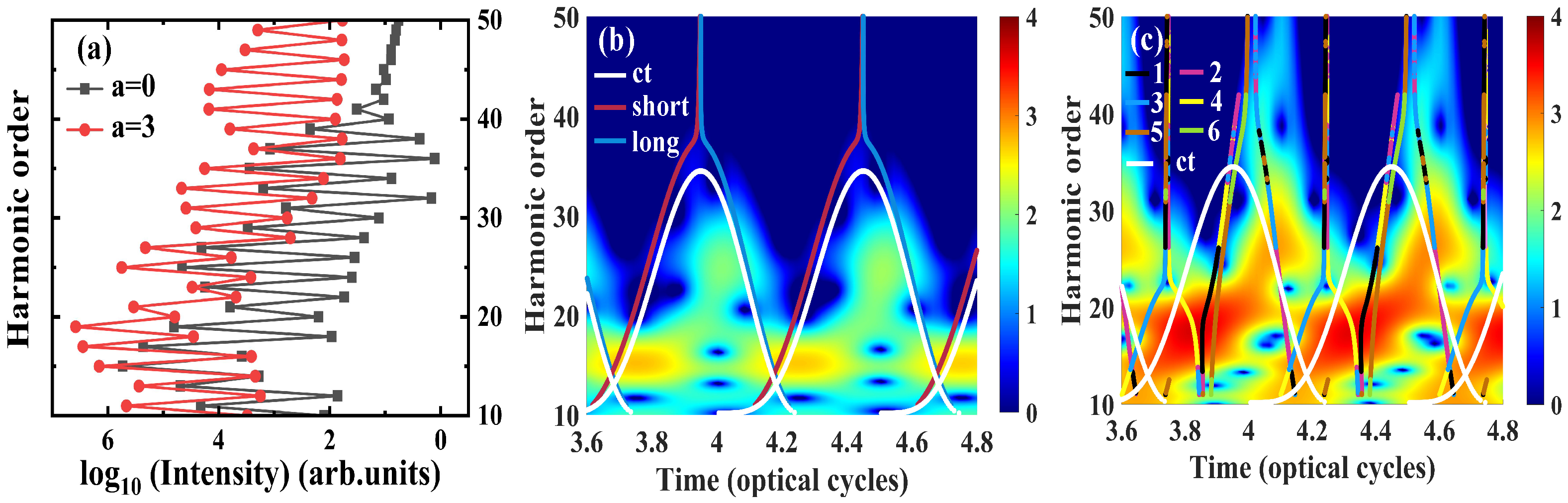
In Figure 2a, we first present the numerical integration of Equation (30) for two representative cases: $a=0$ (without gauge correction) and $a=3$ (with gauge correction). The resulting HHG spectra exhibit a behavior similar to that observed for the iodine molecule. Specifically, the spectrum for $a=3$ is overall stronger compared to the $a=0$ case, whereas the $a=0$ spectrum displays a more pronounced peak-valley structure.

Figure 2. (a) presents the HHG spectra for $a=0$ and $a=3$; the time frequency analysis plots for $a=0$ and $a=3$ are exhibited in (b) and (c) respectively. Furthermore, the white lines in the figures denote classical trajectories, while the colored lines represent quantum orbitals (with two for $a=0$ and six for $a=3$).

From the time–frequency analyses shown in Figure 2b,c, it is evident that for $a=0$, the HHG emission is predominantly governed by the conventional long and short quantum trajectories. In contrast, for $a=3$, additional quantum trajectories emerge, which are particularly pronounced in the range of the 30th–40th harmonics.

Next, we employ the gauge-corrected saddle-point approximation to investigate the underlying physical mechanisms responsible for the differences between these two cases. Applying stationary-phase conditions to the total phase $\Phi =S(\mathbf{k},t,t^{\prime })-\chi \left({\mathbf{q}}_{t^{\prime }}\right)+\chi \left({\mathbf{q}}_t\right)$ (we temporarily neglect phases coming from $\overline{\mathbf{d}}$ and from prefactors—those can be included straightforwardly. A detailed mathematical derivation of this point can be found in the Supplementary Materials. The saddle equations can be expressed as follows:

$$\begin{array}{cc}\hfill {\partial }_{\mathbf{k}}\Phi & ={\int }_{t^{\prime }}^{t}d\tau {\mathbf{q}}_{\tau }-{\nabla }_{\mathbf{k}}\chi \left({\mathbf{q}}_{t^{\prime }}\right)+{\nabla }_{\mathbf{k}}\chi \left({\mathbf{q}}_t\right)=0,\hfill \end{array}$$

(35)

$$\begin{array}{cc}\hfill {\partial }_{t^{\prime }}\Phi & =-{\displaystyle \frac{{\mathbf{q}}_{t^{\prime }}^2}{2}}-I_p-\mathbf{E}\left(t^{\prime }\right)·{\nabla }_{\mathbf{q}}\chi \left({\mathbf{q}}_{t^{\prime }}\right)=0,\hfill \end{array}$$

(36)

$$\begin{array}{cc}\hfill {\partial }_t\Phi & ={\displaystyle \frac{{\mathbf{q}}_t^2}{2}}+I_p-\omega +\mathbf{E}\left(t\right)·{\nabla }_{\mathbf{q}}\chi \left({\mathbf{q}}_t\right)=0.\hfill \end{array}$$

(37)

These equations show explicitly the extra terms proportional to $\mathbf{E}·{\nabla }_{\mathbf{q}}\chi$ which originate from the endpoint phase differences $\chi \left({\mathbf{q}}_{t^{\prime }}\right)-\chi \left({\mathbf{q}}_t\right)$.

The modified saddle-point equations in Equations (35)–(37) reveal the physical role of the nonlocal potential. In the momentum equation, the additional gradient terms ${\nabla }_{\mathbf{k}}\chi \left({\mathbf{q}}_{t^{\prime }}\right)-{\nabla }_{\mathbf{k}}\chi \left({\mathbf{q}}_t\right)$ indicate that the electronic trajectory acquires extra phase distortions from the nonlocal coupling of the initial and final states. Physically, this correction can be interpreted as the so-called “imperfect recombination” of the electron in multi-center molecular systems [54].

In polyatomic molecules, the electron wave packet released by a strong laser field does not necessarily recombine at the same atomic center from which it is tunnel-ionized. Because of the finite spatial extent of molecular orbitals and the multi-center Coulomb potential, the electron can migrate across different atomic sites during its continuum propagation. Such non-local electron dynamics becomes particularly important in situations related to Coulomb explosion, where nuclear displacement enhances charge localization and molecular asymmetry. As a consequence, recombination at a different atomic center becomes both possible and physically relevant.

This multi-center recollision pathway introduces an additional geometric and dynamical phase, which naturally appears as a non-local correction to the dipole phase. In the semiclassical picture, the electron accumulates a phase

$$\mathrm{\Delta }{\varphi }_{\mathrm{nl}}={\int }_{t^{\prime }}^t\mathbf{p}\left(t\right)·d\mathbf{r}\left(t\right),$$

(38)

where $t^{\prime }$ and t denote the ionization and recombination times. When the electron ionizes and recombines at two centers separated by $\mathrm{\Delta }\mathbf{R}$, one obtains an additional phase term

$$\mathrm{\Delta }{\varphi }_{\mathrm{nl}}=\mathbf{k}·\mathrm{\Delta }\mathbf{R},$$

(39)

with $\mathbf{k}$ the canonical momentum at recombination. This term vanishes in atomic systems but becomes significant in heteronuclear or extended molecules.

In the tunneling condition, the correction $-\mathbf{E}\left(t^{\prime }\right)·{\nabla }_{\mathbf{q}}\chi \left({\mathbf{q}}_{t^{\prime }}\right)$ shows that the tunneling barrier is modified by the interplay between the instantaneous field and the spatial structure of the nonlocal potential, thereby influencing both the tunneling probability and the initial phase. Similarly, the recombination condition contains the term $+\mathbf{E}\left(t\right)·{\nabla }_{\mathbf{q}}\chi \left({\mathbf{q}}_t\right)$, which demonstrates that the emitted photon energy and tunneling dynamics are also sensitive to the orbital nonlocality at recombination.

As illustrated in Figure 2b,c, these additional phase terms lead to the emergence of extra quantum trajectories beyond the conventional long and short ones. The interference among multiple trajectories with comparable amplitude reduces overall coherence, weakening the peak-valley structure in the HHG spectra.

For light atoms such as Ar, the corrections are small and the standard long-short trajectory picture remains valid. In contrast, for I₂, the nonlocal effects are pronounced, leading to stronger HHG intensity and more complex trajectory contributions, in agreement with TDDFT results (Figure 1b), confirming the physical relevance of the gauge-corrected SFA.

From a mathematical point of view, in the case of a local potential, the saddle-point equations admit four solutions in the complex plane, which appear in pairs due to the quadratic dependence on $q^2$ [1,55,56]. Physically, these solutions correspond to the long and short trajectories in the classical three-step model, where the imaginary parts of the ionization and recombination times encode the quantum tunneling time associated with different trajectories [57,58,59,60]. In contrast, for a nonlocal potential, the additional phase corrections alter the structure of the equations such that the highest order in p is no longer necessarily quadratic. As a consequence, the saddle-point system may possess more than four solutions, and the pairwise symmetry is lost.

This splitting of the classical long and short trajectories arises from the complex scattering of the electronic wave packet with the multi-center potential or heavy nuclei during ionization and recombination. In such systems, the spatially extended and structured potential enhances the probability of quantum diffraction, thereby generating additional quantum trajectories. As a consequence, the direct correspondence between the classical three-step model and the recombining quantum trajectories breaks down.

Above analysis is supported by the comparison between the classical trajectories and the quantum trajectories obtained from solving the saddle-point equations, as shown in Figure 2b,c. In Figure 2b, the classical trajectories (white solid lines) are in good agreement with the quantum trajectories (colored solid lines). In contrast, in Figure 2c, the quantum trajectories completely lose the characteristic feature of being separated into only long and short trajectories and split into six quantum trajectories.

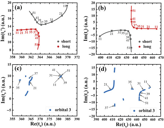
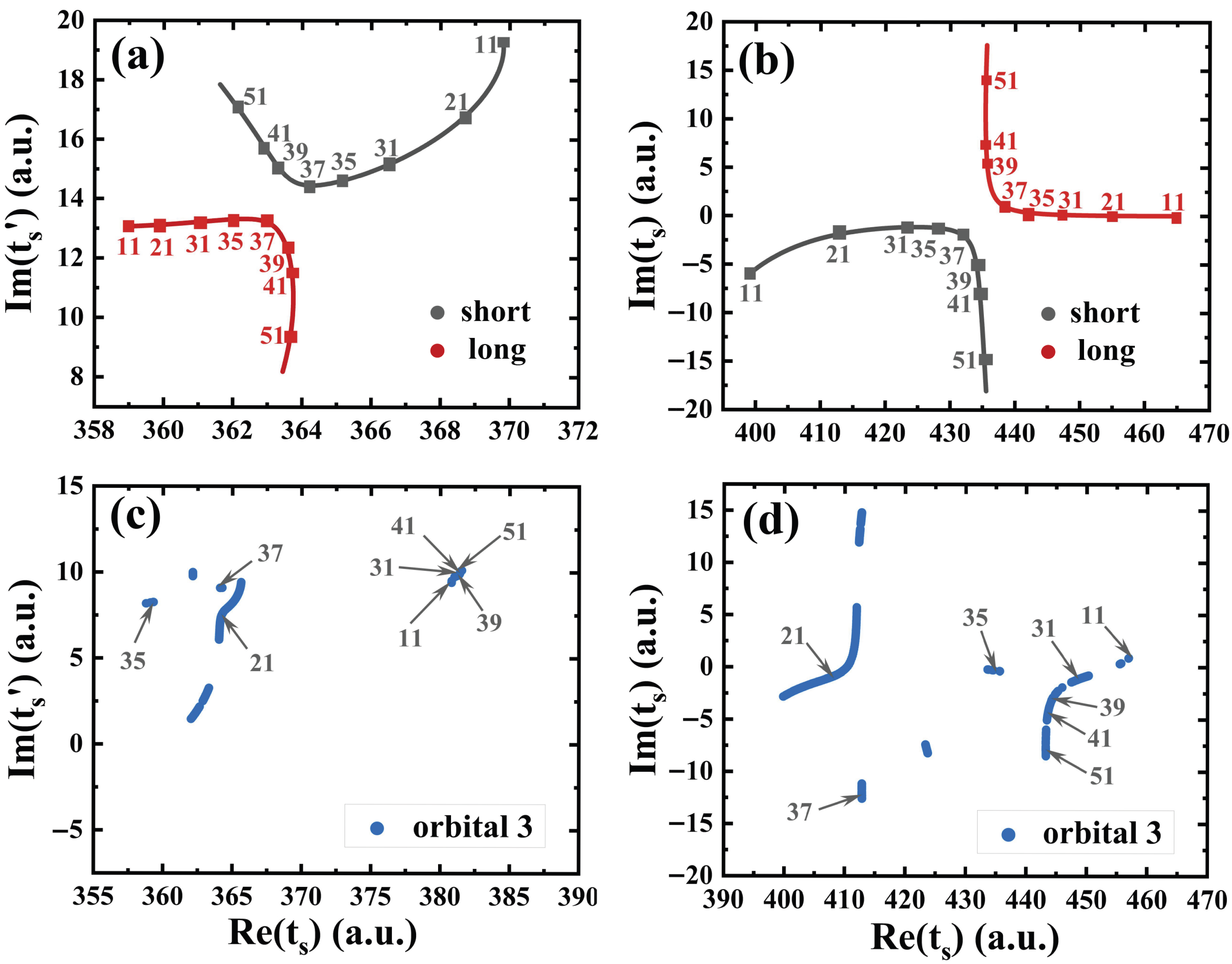
Furthermore, in Figure 3, we present the solutions of the saddle-point equations in the complex plane, showing the phase-space diagrams of $t_s$ and $t_s^{\prime }$ for the cases without gauge correction (panels a and b) and with gauge correction (panels c and d). For the gauge-corrected case, we only display the solutions corresponding to Orbital-3, while the solutions for other trajectories are provided in the Supplementary Materials. According to the saddle-point approximation, the contribution of each quantum trajectory to HHG scales as

$${\mathcal{A}}_s\left(\omega \right)\propto exp\left[-\omega \mathrm{Im}\left(t_s\right)\right],$$

(40)

as shown in Figure 3b, the imaginary part of $t_s$ has a smaller absolute value compared to the corresponding solutions in Figure 3d, which indicates that the HHG intensity with gauge correction is stronger than that without correction. This enhancement originates from the use of nonlocal potentials, which modify the tunneling process of the electron. This analysis explains why the HHG spectra in Figure 2 with gauge correction are stronger than those obtained without correction, especially in the high energy domain.

Figure 3. The saddle-point results for the ionization time $t_s^{\prime }$ and the recollision time $t_s$. (a,b) show the long and short orbital results for $t_s^{\prime }$ and $t_s$ when $a=0$, marked with black dots and red dots, respectively. (c,d) display the results for one orbital (orbital 3) of $t_s^{\prime }$ and $t_s$ when $a=3$, marked with blue dots. (Specific order positions are highlighted with arrows and numbers for clarity.)

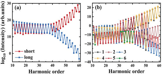
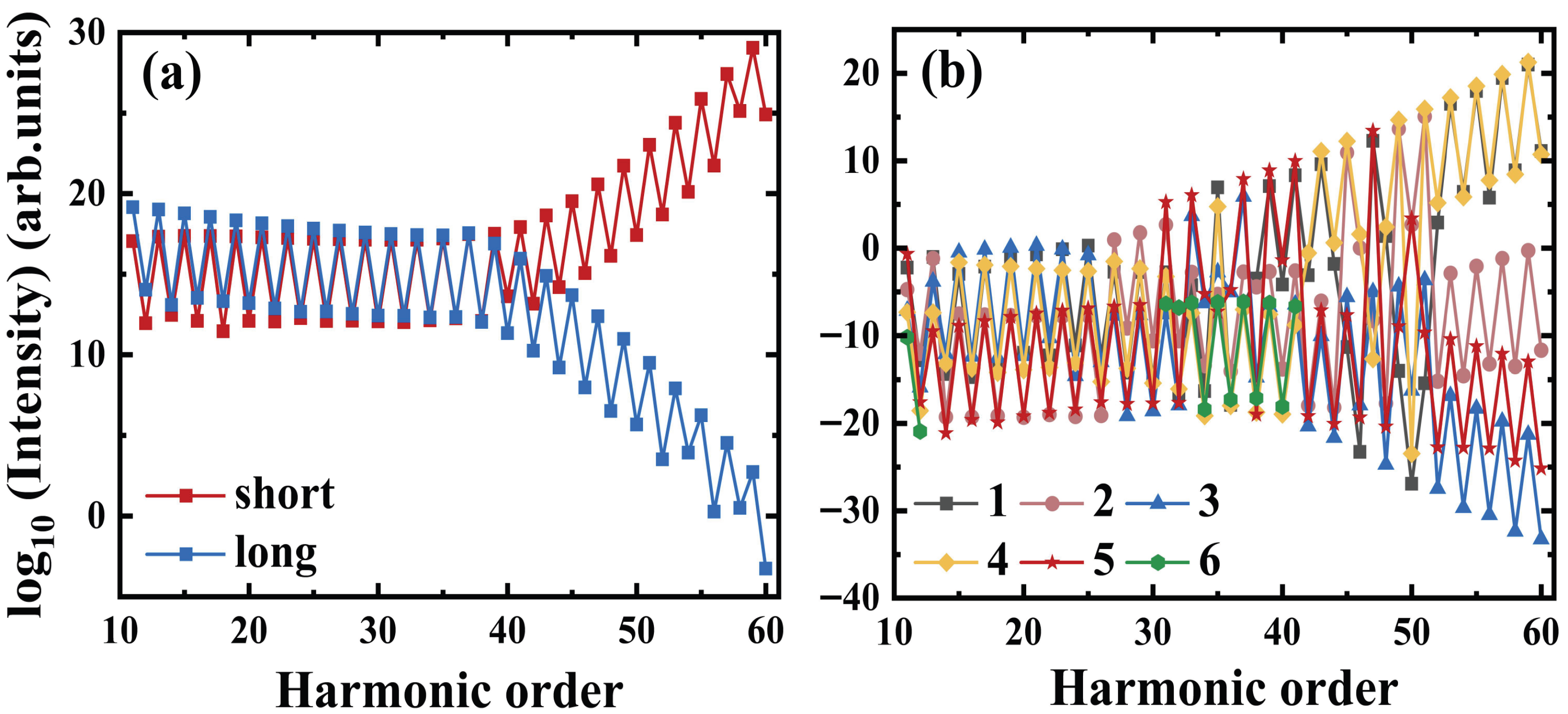
It is well known that the peak-valley structure in HHG spectra arises from the interference of different quantum trajectories. To investigate the influence of the phase correction on this structure, we computed, within the saddle-point approximation, the contributions of each quantum trajectory for the cases $a=0$ and $a=3$. As shown in Figure 4, for $a=0$, only two trajectories, namely the long and short ones, contribute significantly to the total HHG. In contrast, for $a=3$, six quantum trajectories exhibit noticeable contributions. Mathematically, when several complex amplitudes of comparable magnitude are summed, and their phases are distributed in a relatively random manner, the overall coherence decreases with the number of contributing terms. Our example precisely matches this scenario, which explains why the introduction of the gauge correction weakens the peak-valley structure in our case.

Figure 4. Using the numerical solutions at saddle points to calculate quantum orbitals, (a) shows two sub-orbits for $a=0$, indicated in red and blue respectively, while (b) displays six sub-orbits for $a=3$, represented by black, pink, blue, yellow, red, and green, respectively.

4. Summary List

a. 

List of Abbreviations

• ATI—Above-Threshold Ionization
• HF—Hartree–Fock
• LDA—Local Density Approximation
• SBE—Semiconductor Bloch Equations
• TDDFT—Time-Dependent Density Functional Theory
• “sup”—denotes superscript/footnote reference in equations or figure labels
• $arg(·)$—complex argument (phase) of a complex number
• HHG—High-Harmonic Generation

b. 

Definition of Key Parameters

• $\mathbf{d}\left(\mathbf{q}\right)=⟨\mathbf{q}\left|\widehat{\mathbf{r}}\right|0⟩$—length-gauge transition dipole (a.u.).
• $\mathbf{v}\left(\mathbf{q}\right)=⟨\mathbf{q}\left|\widehat{\mathbf{p}}\right|0⟩$—velocity matrix element (a.u.).
• $\mathbf{C}\left(\mathbf{q}\right)=⟨\mathbf{q}\left|\widehat{\mathrm{\Delta }}\right|0⟩$—nonlocal commutator correction vector (a.u.).
• $\chi \left(\mathbf{q}\right)$—additional gauge-dependent dipole phase introduced to model nonlocal effects (radians).
• $R\left(\mathbf{q}\right)\equiv \left|C\left(\mathbf{q}\right)\right|/\left({\omega }_{\mathbf{q}0}\right|d\left(\mathbf{q}\right)\left|\right)$—dimensionless diagnostic measuring the relative strength of nonlocal gauge corrections.
• $I_p$—ionization potential (a.u.).
• $t^{\prime }$ and t—complex ionization time and recombination (recollision) time determined from saddle-point equations.

c. 

Summary of representative $\mathbf{R}\left(\mathbf{q}\right)$ ranges, gauge sensitivity, and HHG spectral characteristics for different systems.

System Class	$\mathit{R}(\mathbf{q})$ (Typical)	Gauge Sensitivity	HHG Signature
Light atoms (e.g., Ar)	<0.1	negligible	Standard short/long trajectories, strong peaks
Typical diatomics (e.g., N2)	$0.1$–$0.8$	moderate	Modified amplitudes, mild interference changes
Heavy multi-center molecules (e.g., I2)	$0.7$–$2.0$	strong	Multiple quantum trajectories, reduced coherence, weaker peak-valley structure

d. 

Summary of the key findings presented in the figures of this paper

• Figure 1—Compared to light atoms like Ar, heavy-atom molecules like I₂ exhibit significant gauge dependence.
• Figure 2—After gauge correction, the overall HHG spectral intensity increases, and the peak-valley structure weakens. Specifically, before correction, HHG emission is dominated by conventional long and short quantum trajectories, consistent with classical trajectories. After correction, additional quantum trajectories emerge, breaking the long/short trajectory symmetry.
• Figure 3—After gauge correction, the smaller absolute value of the imaginary parts in the saddle-point solutions leads to enhanced HHG intensity; the nonlocal potential modifies the electron tunneling process, explaining the enhancement in the high-energy region.
• Figure 4—Before gauge correction, only the long and short trajectories contribute significantly to HHG, and their interference creates a distinct peak-valley structure. After correction, six quantum trajectories with random phase distribution appear, reducing overall coherence and weakening the peak-valley structure.

5. Conclusions

In summary, we have systematically analyzed the effects of nonlocal potentials on the gauge dependence of transition dipole moments within the strong-field approximation framework. We derived the necessary phase corrections in the Volkov action to restore gauge invariance and demonstrated how these corrections modify the semiclassical trajectories and saddle-point equations. Our numerical simulations on Ar and I₂ molecules show that while light-atom systems are largely insensitive to nonlocal effects, heavy-atom molecules exhibit significant deviations that can be corrected using our method. Comparison with TDDFT calculations confirms the physical relevance of the gauge-corrected SFA. This work provides a practical and rigorous framework for accurately modeling strong-field processes in complex molecular systems with SFA model, and highlight that, when applying the SFA to complex molecules with dipoles obtained from nonlocal potentials, gauge-related issues cannot be neglected. Finally, we emphasize that the “gauge covariance of nonlocal potentials” and the “gauge dependence of the SFA” are fundamentally distinct physical and mathematical questions. The former concerns the construction of a gauge-consistent Hamiltonian with a nonlocal binding potential, while the latter reflects the intrinsic non-gauge-invariant nature of the SFA approximation, even for local potentials. By separating these issues and treating them independently, the present work provides a clearer theoretical framework for understanding gauge-related effects in molecular strong-field physics.

References

- Lewenstein, M.; Balcou, P.; Ivanov, M.Y.; L’huillier, A.; Corkum, P.B. Theory of high-harmonic generation by low-frequency laser fields. Phys. Rev. A 1994, 49, 2117. [Google Scholar] [CrossRef] [Scilit] [PubMed]
- Krausz, F.; Ivanov, M. Attosecond physics. Rev. Mod. Phys. 2009, 81, 163–234. [Google Scholar] [CrossRef] [Scilit]
- Milošević, D.; Paulus, G.; Bauer, D.; Becker, W. Above-threshold ionization by few-cycle pulses. J. Phys. B 2006, 39, R203. [Google Scholar] [CrossRef] [Scilit]
- Becker, W.; Liu, X.; Ho, P.J.; Eberly, J.H. Theories of photoelectron correlation in laser-driven multiple atomic ionization. Rev. Mod. Phys. 2012, 84, 1011–1043. [Google Scholar] [CrossRef] [Scilit]
- Minneker, B.; Böning, B.; Fritzsche, S. Generalized nondipole strong-field approximation of high-order harmonic generation. Phys. Rev. A 2022, 106, 053109. [Google Scholar] [CrossRef] [Scilit]
- Jiang, S.; Wei, H.; Chen, J.; Yu, C.; Lu, R.; Lin, C. Effect of transition dipole phase on high-order-harmonic generation in solid materials. Phys. Rev. A 2017, 96, 053850. [Google Scholar] [CrossRef] [Scilit]
- Wu, D.; Li, L.; Zhan, Y.; Huang, T.; Cui, H.; Li, J.; Lan, P.; Lu, P. Determination of transition dipole moments of solids with high-order harmonics driven by multicycle ultrashort pulses. Phys. Rev. A 2022, 105, 063101. [Google Scholar] [CrossRef] [Scilit]
- Zhao, X.; Wei, H.; Wu, Y.; Lin, C.D. Phase-retrieval algorithm for the characterization of broadband single attosecond pulses. Phys. Rev. A 2017, 95, 043407. [Google Scholar] [CrossRef] [Scilit]
- Usachenko, V.I.; Chu, S.I. Strong-field ionization of laser-irradiated light homonuclear diatomic molecules: A generalized strong-field approximation–linear combination of atomic orbitals model. Phys. Rev. A 2005, 71, 063410. [Google Scholar] [CrossRef] [Scilit]
- Milošević, D. Strong-field approximation for ionization of a diatomic molecule by a strong laser field. Phys. Rev. A 2006, 74, 063404. [Google Scholar] [CrossRef] [Scilit]
- Amini, K.; Biegert, J.; Calegari, F.; Chacón, A.; Ciappina, M.F.; Dauphin, A.; Efimov, D.K.; de Morisson Faria, C.F.; Giergiel, K.; Gniewek, P.; et al. Symphony on strong field approximation. Rep. Prog. Phys. 2019, 82, 116001. [Google Scholar] [CrossRef] [Scilit] [PubMed]
- Salamin, Y.I.; Hu, S.; Hatsagortsyan, K.Z.; Keitel, C.H. Relativistic high-power laser–matter interactions. Phys. Rep. 2006, 427, 41–155. [Google Scholar] [CrossRef] [Scilit]
- Le, A.T.; Wei, H.; Jin, C.; Lin, C. Strong-field approximation and its extension for high-order harmonic generation with mid-infrared lasers. J. Phys. B 2016, 49, 053001. [Google Scholar] [CrossRef] [Scilit]
- Shao, Y.; Molnar, L.F.; Jung, Y.; Kussmann, J.; Ochsenfeld, C.; Brown, S.T.; Gilbert, A.T.; Slipchenko, L.V.; Levchenko, S.V.; O’Neill, D.P.; et al. Advances in methods and algorithms in a modern quantum chemistry program package. Phys. Chem. Chem. Phys. 2006, 8, 3172–3191. [Google Scholar] [CrossRef] [Scilit]
- Karlström, G.; Lindh, R.; Malmqvist, P.Å.; Roos, B.O.; Ryde, U.; Veryazov, V.; Widmark, P.O.; Cossi, M.; Schimmelpfennig, B.; Neogrady, P.; et al. MOLCAS: A program package for computational chemistry. Comput. Mater. Sci. 2003, 28, 222–239. [Google Scholar] [CrossRef] [Scilit]
- Shao, Y.; Gan, Z.; Epifanovsky, E.; Gilbert, A.T.; Wormit, M.; Kussmann, J.; Lange, A.W.; Behn, A.; Deng, J.; Feng, X.; et al. Advances in molecular quantum chemistry contained in the Q-Chem 4 program package. Mol. Phys. 2015, 113, 184–215. [Google Scholar] [CrossRef] [Scilit]
- Baerends, E.; Gritsenko, O.; Van Meer, R. The Kohn–Sham gap, the fundamental gap and the optical gap: The physical meaning of occupied and virtual Kohn–Sham orbital energies. Phys. Chem. Chem. Phys. 2013, 15, 16408–16425. [Google Scholar] [CrossRef] [Scilit]
- Yamazaki, M.; Horio, T.; Kishimoto, N.; Ohno, K. Determination of outer molecular orbitals by collisional ionization experiments and comparison with Hartree-Fock, Kohn-Sham, and Dyson orbitals. Phys. Rev. A 2007, 75, 032721. [Google Scholar] [CrossRef] [Scilit]
- Wang, B.; Zhang, Q.; Zhu, X.; Lan, P.; Rezvani, S.A.; Lu, P. Asymmetric molecular-orbital tomography by manipulating electron trajectories. Phys. Rev. A 2017, 96, 053406. [Google Scholar] [CrossRef] [Scilit]
- Jin, C.; Wang, S.J.; Zhao, X.; Zhao, S.F.; Lin, C. Shaping attosecond pulses by controlling the minima in high-order harmonic generation through alignment of CO2 molecules. Phys. Rev. A 2020, 101, 013429. [Google Scholar] [CrossRef] [Scilit]
- Zhao, X.; Wei, H.; Yu, W.W.; Lin, C. Reconstruction of the complex angle-dependent photoionization transition dipole from a laser-dressed streaking experiment. Phys. Rev. A 2018, 98, 053404. [Google Scholar] [CrossRef] [Scilit]
- Evens, D.; Moffat, J.; Kleppe, G.; Woodard, R. Nonlocal regularizations of gauge theories. Phys. Rev. D 1991, 43, 499. [Google Scholar] [CrossRef] [Scilit] [PubMed]
- Yang, K.H. The physics of gauge transformations. Am. J. Phys. 2005, 73, 742–751. [Google Scholar] [CrossRef] [Scilit]
- Jackson, J.D. From Lorenz to Coulomb and other explicit gauge transformations. Am. J. Phys. 2002, 70, 917–928. [Google Scholar] [CrossRef] [Scilit]
- Reiss, H.R. Gauges for intense-field electrodynamics. Phys. Rev. A 1980, 22, 770. [Google Scholar] [CrossRef] [Scilit]
- Reiss, H.R.; Krainov, V.P. Coulomb-Volkov correction for a strong-field approximation. In Proceedings of the ICONO’95: Fundamentals of Laser-Matter Interaction, St. Petersburg, Russia, 27 June–1 July 1995; SPIE: Bellingham, WA, USA, 1996; Volume 2796, pp. 39–44. [Google Scholar] [CrossRef] [Scilit]
- Faisal, F. Gauge-equivalent intense-field approximations in velocity and length gauges to all orders. Phys. Rev. A At. Mol. Opt. Phys. 2007, 75, 063412. [Google Scholar] [CrossRef] [Scilit]
- Faisal, F. Gauge-invariant intense-field approximations to all orders. J. Phys. B At. Mol. Opt. Phys. 2007, 40, F145. [Google Scholar] [CrossRef] [Scilit]
- Mishra, M.; Yadav, D.; Sharma, M.; Rajan, M.S.M.; Dhasarathan, V. Hyper-gaussian beams for power reduction in nonlocal nonlinear optical systems. Phys. Scr. 2025, 100, 075126. [Google Scholar] [CrossRef] [Scilit]
- Gazibegović-Busuladžić, A.; Milošević, D.; Becker, W. Gauge dependence of the strong-field approximation: Theory vs. experiment for photodetachment of F−. Opt. Commun. 2007, 275, 116–122. [Google Scholar] [CrossRef] [Scilit]
- Rensink, T.; Antonsen, T., Jr. Strong-field ionization and gauge dependence of nonlocal potentials. Phys. Rev. A 2016, 94, 063407. [Google Scholar] [CrossRef] [Scilit]
- Li, J.; Zhang, X.; Fu, S.; Feng, Y.; Hu, B.; Du, H. Phase invariance of the semiconductor Bloch equations. Phys. Rev. A 2019, 100, 043404. [Google Scholar] [CrossRef] [Scilit]
- Milošević, D.; Jašarević, A.; Habibović, D.; Hasović, E.; Čerkić, A.; Becker, W. Asymptotic methods applied to integrals occurring in strong-laser-field processes. J. Phys. A Math. Theor. 2024, 57, 393001. [Google Scholar] [CrossRef] [Scilit]
- Liu, J.; Jiang, S.; Chen, J.; He, L.; Wang, J.; Zhao, X. Complex saddle point analysis of solid high order harmonic generation and reconstruction of dephasing time. APL Comput. Phys. 2025, 1, 026104. [Google Scholar] [CrossRef] [Scilit]
- Schwerdtfeger, P. The pseudopotential approximation in electronic structure theory. ChemPhysChem 2011, 12, 3143–3155. [Google Scholar] [CrossRef] [Scilit] [PubMed]
- Weeks, J.D.; Rice, S.A. Use of pseudopotentials in atomic-structure calculations. J. Chem. Phys. 1968, 49, 2741–2755. [Google Scholar] [CrossRef] [Scilit]
- Baldo, M.; Elgarøy, Ø.; Engvik, L.; Hjorth-Jensen, M.; Schulze, H.J. 3P2-3F2 pairing in neutron matter with modern nucleon-nucleon potentials. Phys. Rev. C 1998, 58, 1921. [Google Scholar] [CrossRef] [Scilit]
- Teale, A.M.; Helgaker, T.; Savin, A.; Adamo, C.; Aradi, B.; Arbuznikov, A.V.; Ayers, P.W.; Baerends, E.J.; Barone, V.; Calaminici, P.; et al. DFT exchange: Sharing perspectives on the workhorse of quantum chemistry and materials science. Phys. Chem. Chem. Phys. 2022, 24, 28700–28781. [Google Scholar] [CrossRef] [Scilit]
- Ozaki, T.; Toyoda, M. Accurate finite element method for atomic calculations based on density functional theory and Hartree–Fock method. Comput. Phys. Commun. 2011, 182, 1245–1252. [Google Scholar] [CrossRef] [Scilit]
- Peierls, R. Zur theorie des diamagnetismus von leitungselektronen. Z. Phys. 1933, 80, 763–791. [Google Scholar] [CrossRef] [Scilit]
- Schwinger, J. On gauge invariance and vacuum polarization. Phys. Rev. 1951, 82, 664. [Google Scholar] [CrossRef] [Scilit]
- Chretien, M.; Peierls, R.E. A study of gauge-invariant non-local interactions. Proc. R. Soc. Lond. 1954, 223, 468–481. [Google Scholar] [CrossRef] [Scilit]
- Wilson, K.G. Confinement of quarks. Phys. Rev. D 1974, 10, 2445. [Google Scholar] [CrossRef] [Scilit]
- Weiss, N. Wilson line in finite-temperature gauge theories. Phys. Rev. D 1982, 25, 2667. [Google Scholar] [CrossRef] [Scilit]
- Kiskis, J. Phase of the Wilson line. Phys. Rev. D 1995, 51, 3781. [Google Scholar] [CrossRef] [Scilit]
- Pisarski, R.D. Effective theory of Wilson lines and deconfinement. Phys. Rev. D Part. Fields Gravit. Cosmol. 2006, 74, 121703. [Google Scholar] [CrossRef] [Scilit]
- Bauer, D.; Milošević, D.; Becker, W. Strong-field approximation for intense-laser–atom processes: The choice of gauge. Phys. Rev. A 2005, 72, 023415. [Google Scholar] [CrossRef] [Scilit]
- Yue, L.; Gaarde, M.B. Structure gauges and laser gauges for the semiconductor Bloch equations in high-order harmonic generation in solids. Phys. Rev. A 2020, 101, 053411. [Google Scholar] [CrossRef] [Scilit]
- Parks, A.; Moloney, J.; Brabec, T. Gauge invariant formulation of the semiconductor Bloch equations. Phys. Rev. Lett. 2023, 131, 236902. [Google Scholar] [CrossRef] [Scilit]
- Parks, A.; Moloney, J.; Brabec, T. Bloch gauge symmetry of the semiconductor Bloch equations. J. Opt. Soc. Am. B 2024, 41, B47–B59. [Google Scholar] [CrossRef] [Scilit]
- Castro, A.; Appel, H.; Oliveira, M.; Rozzi, C.A.; Andrade, X.; Lorenzen, F.; Marques, M.A.; Gross, E.; Rubio, A. Octopus: A tool for the application of time-dependent density functional theory. Phys. Status Solidi b 2006, 243, 2465–2488. [Google Scholar] [CrossRef] [Scilit]
- Marques, M.A.; Castro, A.; Bertsch, G.F.; Rubio, A. Octopus: A first-principles tool for excited electron–ion dynamics. Comput. Phys. Commun. 2003, 151, 60–78. [Google Scholar] [CrossRef] [Scilit]
- Zhou, S.S.; Li, Y.L.; Zhao, Z.X.; Xing, M.; Xu, N.; Wang, H.; Wang, J.; Zhao, X.; Hu, M.H. High-order harmonic generation of methane in an elliptically polarized field. Chin. Phys. B 2025, 34, 063202. [Google Scholar] [CrossRef] [Scilit]
- Brown, G.G.; Ko, D.H.; Zhang, C.; Corkum, P.B. Attosecond measurement via high-order harmonic generation in low-frequency fields. Phys. Rev. A 2022, 105, 023520. [Google Scholar] [CrossRef] [Scilit]
- Ye, D.F.; Chen, J.; Liu, J. Classical trajectory perspective on double-ionization dynamics of diatomic molecules irradiated by ultrashort intense laser pulses. Phys. Rev. A 2008, 77, 013403. [Google Scholar] [CrossRef] [Scilit]
- Kovacs, K.; Toşa, V. Quantum trajectories of electrons in arbitrary laser fields. J. Mod. Opt. 2010, 57, 977–983. [Google Scholar] [CrossRef] [Scilit]
- Steingasser, T.; Kaiser, D.I. Toward quantum tunneling from excited states: Recovering imaginary-time instantons from a real-time analysis. Phys. Rev. D 2025, 111, 096009. [Google Scholar] [CrossRef] [Scilit]
- Popov, V. Imaginary-time method in quantum mechanics and field theory. Phys. At. Nucl. 2005, 68, 686–708. [Google Scholar] [CrossRef] [Scilit]
- Garashchuk, S. Quantum trajectory dynamics in imaginary time with the momentum-dependent quantum potential. J. Chem. Phys. 2010, 132, 014112. [Google Scholar] [CrossRef] [Scilit]
- Maji, K.; Mondal, C.; Bhattacharyya, S. Tunnelling time and tunnelling dynamics. Int. Rev. Phys. Chem. 2007, 26, 647–670. [Google Scholar] [CrossRef] [Scilit]
Disclaimer/Publisher’s Note: The statements, opinions and data contained in all publications are solely those of the individual author(s) and contributor(s) and not of MDPI and/or the editor(s). MDPI and/or the editor(s) disclaim responsibility for any injury to people or property resulting from any ideas, methods, instructions or products referred to in the content. |
© 2025 by the authors. Licensee MDPI, Basel, Switzerland. This article is an open access article distributed under the terms and conditions of the Creative Commons Attribution (CC BY) license (https://creativecommons.org/licenses/by/4.0/).