


Abstract
Understanding and improving web performance is essential for enhancing user experience, yet existing approaches remain largely correlation-based and lack causal interpretability. To address this limitation, we propose a causal-inference-driven framework for diagnosing and optimizing user-centric Web Vitals such as Largest Contentful Paint (LCP), First Input Delay (FID), and Cumulative Layout Shift (CLS). Our contributions are threefold. (1) We construct a comprehensive feature representation that captures Document Object Model (DOM) structure, resource loading behaviors, rendering characteristics, and JavaScript execution, integrating browser-level domain knowledge into the modeling pipeline. (2) We introduce a hybrid causal discovery method that combines constraint-based reasoning with differentiable score-based learning to estimate high-dimensional causal structures reflecting real rendering processes. (3) We develop a causal-effect-based intervention optimization module that leverages counterfactual reasoning to identify actionable modifications for performance improvement. Our framework further leverages structural symmetries inherent in rendering processes, using repeated layout patterns and invariant dependency flows to reduce redundancy and strengthen the stability and identifiability of causal discovery. Extensive experiments on HTTP Archive, Chrome UX Report (CrUX), and a synthetic ground truth dataset demonstrate that our framework achieves higher causal accuracy, more stable predictive performance, more effective intervention recommendations, and improved interpretability compared with existing rule-based, statistical, and machine learning baselines. These results highlight the potential of causality-aware analysis for practical web performance optimization.
1. Introduction
Web performance has emerged as a critical determinant of user experience, business outcomes, and digital accessibility in the modern Internet ecosystem. Studies have demonstrated that even marginal improvements in page load time can yield substantial impacts. For example, a 100-millisecond reduction in load time can increase conversion rates by 1% [1], while pages loading within 5 s achieve 70% longer average sessions compared to slower counterparts [2]. As web applications grow increasingly complex—with the median webpage now exceeding 2 MB in size and incorporating hundreds of resources [3]—the challenge of maintaining optimal performance has intensified proportionally.
Contemporary web performance optimization practices rely predominantly on two paradigms: reactive monitoring through Real User Monitoring (RUM) systems [4,5] and heuristic-based optimization guidelines [6,7]. While these approaches have proven valuable, they exhibit fundamental limitations. Monitoring systems identify performance degradation post-factum but provide limited insight into causal mechanisms, forcing developers into trial-and-error remediation cycles. Conversely, best-practice guidelines—such as those codified in Google’s Web Vitals initiative [8]—offer general recommendations that may not account for the intricate interactions within specific web architectures. Recent machine learning approaches have attempted predictive performance modeling [9,10,11], yet these methods predominantly function as black-box predictors, forecasting metrics like Largest Contentful Paint (LCP), First Input Delay (FID), and Cumulative Layout Shift (CLS) without elucidating why performance degrades or which specific code patterns require modification.
The fundamental gap in existing methodologies lies in the absence of causal understanding. Correlation-based models can predict that pages with certain Document Object Model (DOM) characteristics exhibit poor LCP scores, but cannot determine whether modifying those characteristics will causally improve performance. This distinction is critical: spurious correlations abound in web performance data due to confounding factors such as network conditions, device capabilities, and user behavior patterns [12,13]. For instance, a model might observe that pages with large hero images correlate with high LCP values, yet fail to recognize that the causal factor is not image size per se, but rather the absence of preload directives or inefficient critical rendering path construction [14]. Beyond causal relations, modern webpages also exhibit structural symmetry, such as repeated DOM subtrees, symmetric layout blocks, and invariant rendering dependencies, which, when exploited, can reduce effective model complexity and stabilize causal discovery across diverse architectures.
To address these limitations, we propose a paradigm shift from predictive modeling to causal-inference-driven performance engineering. Our framework constructs explicit structural causal models (SCMs) [15] that represent the generative process by which DOM structures, resource loading patterns, and browser rendering behaviors collectively determine observable performance metrics. By leveraging causal discovery algorithms [16,17] on large-scale observational data from the HTTP Archive [3] and the Chrome User Experience Report (CrUX) [18], we learn directed acyclic graphs (DAGs) encoding relationships such as “asynchronous script placement → reduced render-blocking → improved LCP” with quantified effect sizes.
The key innovation of our approach lies in transforming causal graphs into actionable optimization strategies through three mechanisms, as follows:
(1) Counterfactual Reasoning: Rather than relying on costly A/B testing, we employ do-calculus [15] to estimate intervention effects. Given a webpage’s current state, we can answer queries like “What would LCP be if we applied lazy loading to below-the-fold images?” by computing counterfactual quantities , enabling risk-free exploration of optimization alternatives.
(2) Minimal Intervention Set Identification: Not all performance issues warrant equal attention. We formalize the optimization problem as identifying the minimal set of code modifications that maximizes the causal impact on target metrics, subject to implementation-cost constraints. This reduces the overwhelming space of potential optimizations (e.g., 47 distinct recommendations from Lighthouse [19]) to a prioritized, manageable subset with provable performance guarantees.
(3) Robustness to Confounding: Web performance data suffers from pervasive confounding—network latency, device heterogeneity, CDN variations, and user interaction patterns all influence metrics [12,20]. Our framework employs instrumental variable methods [21] and front-door adjustment [15] to recover causal effects even when unmeasured confounders exist, ensuring recommendations remain valid across deployment contexts.
Specifically, this work makes the following contributions:
- We construct a comprehensive feature representation that incorporates DOM structure, resource loading behaviors, rendering characteristics, and JavaScript execution signals, while integrating browser-level domain knowledge into web performance modeling.
- We propose a hybrid causal discovery method that combines constraint-based reasoning (PC algorithm [16]), score-based approaches (GES [22]), with differentiable score-based learning to recover high-dimensional causal structures that reflect real browser rendering processes.
- We develop a causal-effect-based intervention optimization module that leverages counterfactual reasoning to identify actionable performance improvements for key Web Vitals.
- We conduct extensive experiments on HTTP Archive, Chrome UX Report (CrUX), and a synthetic ground truth dataset, demonstrating improvements in causal accuracy, predictive robustness, interpretability, and optimization effectiveness over rule-based and machine learning baselines.
To guide readers through the paper, we will briefly summarize its structure. Section 2 reviews related work on web performance analysis, causal inference in software systems, and explainable machine learning, and positions our contribution with respect to existing rule-based, predictive, and causal approaches. Section 3 introduces the necessary preliminaries, including Web Vitals metrics, structural causal models, and intervention theory, which form the mathematical foundation of our framework. Section 4 presents the proposed causal-inference-driven framework in detail. Section 4.1 describes feature extraction and the incorporation of browser-level domain knowledge. Section 4.2 introduces our hybrid causal discovery algorithm with structural constraints. Section 4.3 covers counterfactual effect estimation. Section 4.4 formulates the intervention optimization problem and solution. Section 4.5 integrates these components into an end-to-end pipeline. Section 5 reports comprehensive experiments on the HTTP Archive, CrUX, and synthetic datasets, including causal discovery accuracy, predictive performance, intervention effectiveness, and interpretability analyses that are structured around four research questions. Section 6 discusses limitations, broader implications, and potential extensions of our approach, and concludes the paper.
2. Related Works
Our work intersects three research domains, as follows: web performance optimization, causal inference in software systems, and explainable machine learning. We review representative efforts in each area and highlight how our approach addresses limitations in prior work.
2.1. Web Performance Measurement and Optimization
Web performance optimization has evolved through several generations of tools and methodologies. Early work by Souders [7] established foundational heuristics such as minimizing HTTP requests, leveraging browser caching, and optimizing critical rendering paths. Grigorik [6] extended these principles with deep analyses of network protocols and browser internals. While invaluable, these expert-crafted guidelines lack adaptability to diverse web architectures and cannot quantify their individual contributions to overall performance.
The advent of Real User Monitoring (RUM) enabled data-driven performance analysis at scale. Gao et al. [4] demonstrated that crowdsourced QoE measurements could reveal performance bottlenecks invisible to synthetic testing. Butkiewicz et al. [12] introduced Klotski, a system that reprioritizes web content for mobile devices by analyzing dependency graphs, achieving significant improvements in above-the-fold rendering. However, these approaches remain reactive, diagnosing problems after deployment rather than predicting performance during development.
Recent efforts have applied machine learning to performance prediction [23,24]. Wang et al. [9] developed WProf to demystify page load performance through detailed causality graphs of resource dependencies, yet their approach focuses on micro-level resource timing rather than macro-level code pattern effects. Netravali et al. [10] proposed Prophecy, which accelerates mobile page loads using final-state write logs to precompute rendering outcomes. While innovative, Prophecy requires server-side modifications and does not generalize across diverse web properties. Kelton et al. [20] leveraged eye-tracking data to optimize perceived performance, but their method depends on expensive user studies unsuitable for continuous optimization.
The introduction of Web Vitals [8] standardized performance metrics around user-centric measurements—LCP, FID, and CLS. Tools like Lighthouse [19] provide automated audits against these metrics, generating comprehensive reports with optimization suggestions. However, Lighthouse’s recommendations are rule-based and non-personalized; developers receive dozens of suggestions without clear prioritization or understanding of interdependencies.
Despite the progress outlined above, several fundamental challenges remain unresolved in web performance modeling. First, existing tools and learning-based methods are primarily correlation-driven—they can highlight performance bottlenecks, but rarely reveal the underlying causal mechanisms that determine how DOM structure, resource loading, and JavaScript execution jointly influence user-centric Web Vitals. Second, the highly heterogeneous nature of modern websites, spanning diverse frameworks, device profiles, and network conditions, makes it difficult for rule-based or purely statistical models to generalize reliably across real-world scenarios. Third, interactions among layout, rendering, and script execution are inherently nonlinear and often involve latent dependencies that cannot be reconstructed from heuristic analyses alone. Finally, most current optimization tools provide long lists of independent suggestions without quantifying their true impact, leaving developers uncertain about which interventions matter most. These challenges motivate the need for a principled modeling framework capable of capturing causal relationships, reasoning about intervention effects, and providing interpretable, actionable guidance at scale. Our work differs fundamentally by learning causal relationships from data, enabling personalized, quantitatively justified optimization strategies.
2.2. Causal Inference and Discovery
Causal inference has traditionally focused on domains with controlled experiments, but recent advances enable causal reasoning from observational data [25]. Pearl’s seminal framework [15] formalized causality through structural causal models (SCMs) and the do-calculus, providing a rigorous mathematical foundation for reasoning about interventions. Spirtes et al. [16] developed constraint-based algorithms (e.g., PC algorithm) for causal discovery, while Chickering [22] introduced score-based methods (e.g., GES) that optimize global graph structures.
Applications of causal inference in software engineering remain nascent. Pandey et al. [26] applied causal analysis to understand user engagement in mobile apps, identifying feature combinations that causally drive retention. Rahman et al. [27] used causal models to predict software defects, demonstrating superior interpretability compared to traditional machine learning. However, these works address post-deployment analysis rather than performance optimization, and none tackle the unique challenges of web environments: high-dimensional feature spaces, complex confounding from network and device heterogeneity, and the need for actionable interventions.
In the systems domain, Gan et al. [28] introduced Seer, a causal framework for diagnosing microservice performance anomalies. Their approach constructs causal graphs among service components but assumes static system architectures, whereas web performance involves dynamic interactions between client-side code, browser engines, and network conditions. Our work extends causal discovery to the web domain by incorporating browser rendering theory as structural constraints, significantly improving discovery accuracy in high-noise environments. These structural constraints also capture inherent symmetries in rendering behaviors, helping the discovery process avoid redundant or directionally equivalent causal patterns.
Recent work in causal reinforcement learning [29,30,31,32] has shown promise for policy optimization under confounding, but these methods require environment simulators, which are impractical for web performance, where browser rendering is too complex for accurate simulation. We instead employ offline causal inference techniques, leveraging instrumental variables [21] to handle unmeasured confounders without requiring environment models.
2.3. Explainable AI and Interpretable Machine Learning
Although explainable AI and interpretable machine learning are general methodological topics, they are directly relevant to web performance modeling. Modern web performance involves complex interactions among DOM structure, resource loading, and rendering processes, making post hoc transparency insufficient for diagnosing bottlenecks or generating actionable recommendations. Therefore, understanding the strengths and limitations of existing interpretability techniques is essential for motivating a causal framework that provides structured and actionable explanations aligned with browser semantics. In fact, the push for explainable AI has produced numerous techniques for interpreting black-box models. Ribeiro et al. [33] proposed LIME (Local Interpretable Model-agnostic Explanations), which approximates complex models locally with interpretable surrogates. Lundberg and Lee [34] introduced SHAP (SHapley Additive exPlanations), grounding feature importance in cooperative game theory. While these methods provide post hoc explanations, they do not guarantee causal validity, as high SHAP values indicate correlation, not causation [35].
Attention mechanisms in neural networks [36,37] offer another interpretability paradigm, highlighting which inputs influence outputs. Vig et al. [38] demonstrated that attention weights in transformers can reveal linguistic structures, but similar analyses for performance modeling remain unexplored. Moreover, attention-based explanations suffer from instability and lack prescriptive value: knowing which DOM elements the model “attended to” does not inform developers how to modify code for improvement.
Counterfactual explanations [39,40] represent a more actionable paradigm, answering “what if” questions about alternative inputs. Sahil et al. [41] applied counterfactuals to software testing, generating minimal input changes that alter program behavior. However, these methods typically rely on differentiable models and continuous input spaces, ill-suited for discrete code patterns in web performance contexts [42,43].
Our approach bridges causal inference and explainability by grounding explanations in structural causal models rather than post hoc approximations. Unlike LIME or SHAP, which identify correlative features, our framework traces causal pathways (e.g., “script placement → parse blocking → delayed LCP”), enabling developers to understand mechanisms and predict intervention outcomes with theoretical guarantees.
Web performance arises from complex interactions among the Document Object Model (DOM), network behavior, rendering dependencies, and JavaScript execution. Existing methods are predominantly correlation-based and often fail to reveal causal mechanisms or provide actionable guidance. The high dimensionality, heterogeneity, and nonlinearity of web data further limit the stability and interpretability of predictions. These challenges motivate the need for a causal and interpretable framework capable of producing reliable and actionable performance insights.
2.4. Positioning of Our Work
While prior work has made significant strides in web performance optimization, causal discovery, and explainable AI independently, no existing framework integrates these paradigms for performance engineering. Table 1 summarizes key differences between our approach and representative prior systems.
Table 1.
Comparison of our approach with existing web performance methodologies.
Our contributions advance the state-of-the-art in three dimensions, as follows: (1) we develop domain-specific causal discovery algorithms that incorporate browser rendering semantics, achieving superior accuracy on web performance data; (2) we formalize intervention identification as an optimization problem with cost constraints, producing minimal actionable recommendations; (3) we demonstrate scalability to millions of real-world webpages while maintaining interpretability—a feat unachievable by existing causal or explainability methods. These innovations establish a new research direction at the intersection of causal AI and web systems engineering.
3. Preliminaries
This section introduces the mathematical foundations that support our predictive optimization framework. In this work, “predictive optimization” refers to improving Web Vitals by learning a structural model that can (i) predict how performance metrics respond to changes in page structure, resource loading, or script execution, and (ii) identify interventions that lead to optimized outcomes based on these predicted effects. Accordingly, the formulations presented in Section 3 and Section 4 describe the components of this pipeline—structural causal modeling, causal effect estimation, and intervention selection. These equations are therefore not stand-alone theoretical constructs, but the core mechanism through which our framework quantifies performance determinants and recommends actionable optimization strategies.
3.1. Web Performance Metrics
Modern web performance assessment centers on user-centric metrics defined by Google’s Web Vitals initiative [8]. We focus on three core metrics that capture distinct aspects of user experience, as follows:
Largest Contentful Paint (LCP): Measures the render time of the largest content element visible in the viewport, formally defined as follows:
where denotes the set of viewport-visible elements, represents element e’s render timestamp, and computes its pixel dimensions. LCP indicates when the main content becomes visible, with the following thresholds: good ( s), needs improvement ( s– s), and poor ( s).
Cumulative Layout Shift (CLS): Quantifies visual stability by aggregating unexpected layout shifts during page lifetime:
where n is the number of layout shifts, measures the proportion of viewport affected by shift i, and quantifies the maximum movement distance normalized by viewport dimensions. Good CLS scores remain below .
First Input Delay (FID): Captures interactivity by measuring the delay between user input and the browser response:
where marks the timestamp of the first user interaction (click, tap, key press) and indicates when the browser begins processing the event. Good FID remains below 100 ms.
Let denote the set of target metrics. Our framework models each as a function of webpage characteristics encoded in a feature vector .
3.2. Structural Causal Models
Following Pearl’s framework [15], we represent the data-generating process for web performance through structural causal models (SCMs).
Definition 1
(Structural Causal Model). A structural causal model is a tuple where
- is a set of exogenous (unobserved) variables representing external factors (e.g., network latency, device capabilities)
- is a set of endogenous (observed) variables including DOM features and performance metrics
- is a set of functions where each assigns values to based on parents :where denotes the exogenous noise term associated with variable , capturing latent factors and stochastic variability not explained by the observed parent variables .
- is a probability distribution over exogenous variables
Each SCM induces a directed acyclic graph (DAG) where an edge exists if . The graph encodes conditional independence relationships via d-separation [15]. In addition, several rendering-related variables exhibit symmetry constraints, e.g., mirrored layout behaviors or repeated resource-loading patterns. Encoding such symmetry priors into the DAG helps eliminate redundant structures and improves the robustness of causal discovery in high-noise scenarios.
Example 1.
Consider a simplified SCM for LCP:
This model posits that script placement causally affects render-blocking behavior, which in turn influences critical path construction and ultimately determines LCP.
3.3. Interventions and Do-Calculus
The key distinction between causal and statistical models lies in intervention reasoning. An intervention forcibly sets variable X to value x, breaking incoming causal edges in .
Definition 2
(Intervention). Given SCM with graph , the intervened model replaces the structural equation for X with and removes all edges into X, yielding the mutilated graph .
The interventional distribution differs fundamentally from the observational conditional . The former answers “What is the effect of setting X to x?” whereas the latter addresses “What is Y given we observed ?” These coincide only when no confounders affect both X and Y.
Pearl’s do-calculus [15] provides rules for computing interventional distributions from observational data:
Rule 1 (Insertion/Deletion of observations):
Here, Z represents the latent structural representation derived from the observed web performance features. It captures lower-dimensional causal factors that influence the downstream Web Vital Y. The encoder maps observed features into the latent space, while the decoder predicts the corresponding metric responses.
Rule 2 (Action/observation exchange):
Rule 3 (Insertion/deletion of actions):
where denotes the graph with edges into X removed, has edges from X removed, and indicates Y and Z are d-separated by W in graph .
3.4. Causal Discovery from Observational Data
Given observational data where represents features of webpage i and denotes its performance metric, our goal is to recover the underlying causal DAG .
Constraint-based methods such as the PC algorithm [16] iteratively test conditional independence hypotheses:
The algorithm constructs a skeleton graph by removing edges between variables that exhibit conditional independence, then orients edges using v-structure detection and propagation rules.
Score-based methods like GES [22] formulate causal discovery as optimization:
where is the space of DAGs. In this formulation, G denotes the learned causal graph over page-level variables, including DOM structure, resource attributes, and script execution features. The set D refers to the intervention candidates—i.e., modifiable page attributes such as resource priorities, script loading strategies, or element layout configurations—over which optimization is performed. The Score here balances goodness-of-fit with model complexity:
with denoting maximum likelihood parameters and the model dimension.
Identifiability: Observational data alone cannot uniquely determine ; instead, we recover an equivalence class represented by a Completed Partially Directed Acyclic Graph (CPDAG) that encodes all DAGs producing identical conditional independence structures.
3.5. Adjustment Sets and Confounding Control
To estimate causal effects without randomized experiments, we must control for confounders—variables affecting both treatment and outcome.
Definition 3
(Backdoor Criterion). A set of variables satisfies the backdoor criterion relative to in DAG if
- 1.
- No variable in is a descendant of X
- 2.
- blocks all backdoor paths from X to Y (paths with an arrow into X)
When the backdoor criterion holds, the causal effect can be estimated via adjustment:
For settings with unmeasured confounders, we employ alternative identification strategies:
Instrumental Variables: A variable Z serves as an instrument for if (1) Z causally affects X, (2) Z affects Y only through X, and (3) Z shares no confounders with Y. The causal effect can be recovered via two-stage least squares:
Front-door Adjustment: When a mediator M lies on all directed paths from X to Y and satisfies certain conditions, we can compute:
3.6. Counterfactual Reasoning
Beyond predicting effects of interventions, SCMs enable counterfactual queries: “What would metric M have been, had we changed feature X, given the observed values?”
Definition 4
(Counterfactual). The counterfactual denotes the value Y would take if X were set to x, given exogenous variables . The counterfactual distribution is as follows:
Computing counterfactuals requires three steps (abduction–action–prediction):
- Abduction: Infer from observations;
- Action: Modify the model via ;
- Prediction: Compute Y under the modified model.
For linear SCMs, counterfactuals have closed-form solutions. For general nonlinear models, we approximate counterfactuals through sampling or neural causal models.
3.7. Problem Formulation
Given the HTTP Archive and CrUX datasets containing N webpages with feature vectors and performance metrics , we address three interconnected problems, as follows:
Problem 1 (Causal Discovery): Learn the causal DAG encoding structural relationships among DOM features and performance metrics .
Problem 2 (Effect Estimation): For any webpage with features and potential intervention , estimate the causal effect:
Problem 3 (Intervention Optimization): Identify the minimal set of interventions that maximizes performance improvement subject to implementation-cost constraints:
where represents the cost of modifying feature and C is the budget constraint.
These formulations establish the theoretical foundation for our methodology, presented in Section 4.
4. Methodology
Building upon the structural causal model established in Section 3, this section operationalizes the causal relationships formalized therein for empirical estimation and actionable optimization. While Section 3 introduces the structural equations and latent noise terms that govern interactions among web performance variables, this section instantiates these relationships through observable metrics (e.g., ), dependency functions, and algorithmic procedures. These components allow us to estimate causal effects and identify performance-improving interventions, thereby completing the predictive optimization pipeline. We proceed in four stages. Section 4.1 describes how we construct a 347-dimensional feature representation that captures DOM structure, resource loading, rendering behaviors, image optimization, and JavaScript execution, while encoding browser rendering semantics. Section 4.2 presents our hybrid causal discovery algorithm that combines constraint-based and score-based methods under structural priors derived from rendering theory. These priors implicitly encode symmetry in repeated layout and loading sequences, reducing the search space and improving graph stability. Section 4.3 explains how we estimate intervention effects using adjustment sets, doubly robust estimators, and instrumental variables. Section 4.4 formulates intervention selection as a constrained optimization problem and introduces an efficient approximation algorithm. Finally, Section 4.5 integrates these components into a unified end-to-end optimization pipeline.
4.1. Feature Engineering with Domain Knowledge
4.1.1. Motivation for Feature Engineering
Raw webpage data (HTML, CSS, JavaScript) exhibits extreme heterogeneity and high dimensionality. Naively treating DOM nodes or script lines as features yields intractable causal discovery problems with complexity for d features. Moreover, browsers follow specific rendering pipelines (parsing, style computation, layout, paint, composite) that impose physical constraints on causality—e.g., layout cannot causally affect parsing. Incorporating this domain knowledge as structured features and constraints dramatically improves both efficiency and accuracy. We further leverage symmetry in webpage structures, such as recurring DOM motifs and parallel rendering branches, to avoid redundant feature construction and reinforce identifiability during causal discovery.
4.1.2. Feature Categories
We extract features across five categories, each aligned with browser rendering stages:
1. DOM Structural Features (): Tree depth ; total node count ; element type distribution: ; viewport coverage ratio: . Here, area(·) computes the two-dimensional pixel area of a DOM region. The variable visible_nodes denotes the set of DOM nodes whose bounding boxes intersect with the viewport and are not occluded. The viewport corresponds to the visible browser window region on the user’s device. Therefore, quantifies the ratio of visible content to the total viewport space.
2. Resource Loading Features (): Script placement indicators: ; resource sizes: ; critical resource count: where ; third-party dependency ratio: .
3. Rendering Path Features (): Critical path length: in the dependency graph; render-blocking time: ; paint operation count from the rendering trace; layer composition complexity.
4. Image Optimization Features (): Lazy loading coverage: ; image format distribution: ; above-the-fold image size: ; responsive image utilization: presence of srcset attributes.
5. JavaScript Execution Features (): Main thread blocking time: ; long task count: ; third-party script execution time; event listener count and types.
The complete feature vector is .
4.1.3. Structural Constraints from Rendering Theory
Browser rendering follows a deterministic pipeline, inducing temporal and logical constraints on causality:
We encode these constraints as a partial order ≺ over feature categories:
This eliminates physically impossible edges (e.g., LCP cannot cause DOM depth) and reduces the search space by approximately 60%.
4.2. Hybrid Causal Discovery with Structural Priors
4.2.1. Motivation for Hybrid Causal Discovery
Generic causal discovery algorithms such as PC and GES struggle with web performance data due to (1) high dimensionality (); (2) nonlinear relationships (e.g., LCP’s nonlinear dependence on image size); (3) mixed data types (continuous metrics and discrete indicators); and (4) measurement noise from network variability. We address these challenges through a hybrid approach that combines multiple algorithms and incorporates domain constraints.
4.2.2. Algorithm Design
Our causal discovery algorithm, WebCausalDiscover, operates in three phases:
Phase 1: Constraint-Based Skeleton Learning. Algorithm 1 outlines the constraint-based causal discovery step that instantiates the structural dependency assumptions introduced in. Specifically, we adapt the PC algorithm [16] with modifications for robustness. The algorithm progressively removes edges between variables that exhibit conditional independence under the structural model.
| Algorithm 1 Constraint-based skeleton construction |
|
The expression denotes the number of current adjacent variables connected to in the partially constructed graph, excluding . This quantity determines the size of conditioning sets considered during the conditional independence tests in constraint-based causal discovery. For conditional independence testing, we use a robust kernel-based method to handle nonlinear dependencies:
where KCIT (Kernel Conditional Independence Test) computes the following:
with being kernel matrices and the residual projection operator. Here, denotes a conditional independence test that evaluates whether variables and are independent, given conditioning set S using dataset D. We use a statistical test based on partial correlations with a significance threshold , consistent with PC-style causal discovery procedures.
Phase 2: Score-Based Edge Orientation. We employ a modified GES algorithm [22] that optimizes a penalized likelihood score:
The algorithm performs greedy hill-climbing with two operators, as follows:
Forward Phase: Add edges that maximally improve the score:
subject to acyclicity and structural constraint satisfaction.
Backward Phase: Remove edges to simplify the model:
Phase 3: Domain-Guided Refinement. We refine the discovered graph by enforcing additional rendering-specific rules:
Rule 1 (Blocking Transitivity): If script S blocks resource R and R affects metric M, then S must have a path to M:
Rule 2 (Critical Path Dominance): Features on the critical rendering path must have stronger effects on LCP than non-critical features:
Rule 3 (Layout Shift Locality): CLS can only be caused by elements that trigger reflows:
Algorithm 2 shows the complete causal discovery algorithm of WebCausalDiscover, which integrates the above three phases. Notably, corresponds to Algorithm 1 in Phase 1, which discovers the undirected skeleton of the causal graph. It iteratively performs conditional independence tests under a significance threshold , following a variable ordering ≺ to systematically expand conditioning sets.
| Algorithm 2 WebCausalDiscover |
|
4.2.3. Complexity Analysis
Theorem 1.
The time complexity of WebCausalDiscover is where d is the number of features, is the maximum conditioning set size, N is the sample size, and is the number of GES iterations.
Proof.
The skeleton construction phase tests edges with conditioning sets up to size , requiring independence tests per edge. Each test processes N samples. The GES phase evaluates edge additions/deletions per iteration over iterations. Domain rule enforcement requires edge validations. □
In practice, structural constraints reduce from d to approximately , making the algorithm tractable for .
4.3. Counterfactual Effect Estimation
4.3.1. Motivation for Counterfactual Effect Estimation
After discovering the causal graph , we must quantify intervention effects. Traditional A/B testing is expensive and time-consuming for web optimization—testing all 347 features individually would require months. Causal inference enables effect estimation from observational data, providing instant “what-if” predictions.
4.3.2. Adjustment-Based Estimation
For interventions satisfying the backdoor criterion, we estimate effects via g-computation:
where
with being a valid adjustment set found via Algorithm 3.
| Algorithm 3 Minimum adjustment set identification |
|
To estimate the conditional expectation nonparametrically, we employ gradient boosting machines:
where denotes regression trees and denotes learned weights.
4.3.3. Doubly Robust Estimation
To improve robustness against model misspecification, we apply doubly robust (DR) estimation [44]:
where is the estimated treatment propensity, and the bias correction term is as follows:
This estimator remains consistent if either the outcome model or the propensity model is correctly specified.
4.3.4. Instrumental Variable Estimation for Unmeasured Confounding
When unmeasured confounders exist (e.g., unobserved user behavior patterns), we leverage instrumental variables. For web performance, we identify natural instruments:
Example 2.
Geographic CDN assignment serves as an instrument for resource load time. CDN affects load time but influences performance only through load time, not via user behavior.
The two-stage least squares (2SLS) estimator is as follows:
where Z is the instrument, are observed covariates, and estimates the causal effect.
4.3.5. Confidence Intervals via Bootstrap
We quantify estimation uncertainty using a stratified bootstrap:
where is the p-th percentile of bootstrap estimates from resamples.
4.4. Intervention Optimization
4.4.1. Motivation
With effect estimates for all features, developers face a new challenge—deciding which interventions to implement, given limited resources. Changing all 347 features is infeasible. We formalize intervention selection as a constrained optimization problem that balances performance gains against implementation costs. We additionally account for symmetric intervention pathways, which are distinct but structurally equivalent modification routes, thereby ensuring the optimizer does not overpenalize redundant alternatives.
4.4.2. Optimization Problem Formulation
Let be the set of intervenable features. For each , we have:
- Estimated causal effect: ;
- Implementation cost: (developer hours required);
- Confidence interval: ;
We define the intervention optimization problem:
where
- indicates whether to apply intervention j;
- C is the total cost budget;
- encodes conflict constraints (mutually exclusive interventions);
- indexes intervention groups, contains interventions in group k;
- We use conservative estimates to ensure robust recommendations.
Proposition 1.
Problem (38) is NP-hard, reducible from the 0–1 knapsack problem.
Proof.
Setting and yields the knapsack problem, which is known to be NP-hard. □
4.4.3. Approximation Algorithm
We develop a greedy algorithm with theoretical approximation guarantees, as shown in Algorithm 4.
| Algorithm 4 Greedy intervention selection |
|
Theorem 2.
If all constraints are monotone and the effect function is submodular, Algorithm 4 achieves a -approximation to the optimal solution.
Proof.
The proof follows from the diminishing returns property of submodular functions. Each greedy choice maximizes the marginal gain per unit cost. Under submodularity, this strategy guarantees at least of the optimal objective value. □
4.4.4. Integer Programming Formulation
For exact solutions on smaller problem instances, we employ integer linear programming (ILP):
We solve this using branch-and-bound with commercial solvers (e.g., Gurobi) for .
4.4.5. Sensitivity Analysis
To ensure robustness to estimation errors, we perform sensitivity analysis by solving the following:
where is the standard error of and controls conservatism. Recommendations appearing in for all are deemed robust.
4.5. End-to-End Pipeline Integration
Algorithm 5 integrates all components into a complete system, using the learned causal graph to compute causal effects and identify candidate interventions. It operationalizes the effect estimation process described in Section 3 by applying adjustment sets and counterfactual prediction rules. Here, (corresponding to Algorithm 3) identifies a minimal sufficient adjustment set for estimating the causal effect of variable on metric M using the learned causal graph G. This function implements standard backdoor criterion checks to locate non-descendant parent sets that block spurious paths.
| Algorithm 5 CausalWebOptimizer |
|
4.6. Theoretical Guarantees
We establish formal guarantees for our framework:
Theorem 3
(Consistency). Under causal sufficiency (no unmeasured confounders) and faithfulness (the causal graph uniquely determines the conditional independences), as :
Theorem 4
(Effect Estimation). If the adjustment set satisfies the backdoor criterion and outcome models are consistently estimated, then:
Theorem 5
(Intervention Guarantee). For any webpage w with current features , implementing interventions guarantees the following:
with probability , where ϵ accounts for interaction effects.
These theorems provide developers with confidence that our recommendations will yield predicted performance improvements in production deployments.
5. Experiments
This section empirically evaluates our framework along four research questions:
- RQ1 (Causal Discovery Accuracy): How accurately does our algorithm recover true causal relationships compared to baselines?
- RQ2 (Predictive Performance): How well do causal models predict performance metrics compared to state-of-the-art ML models?
- RQ3 (Intervention Effectiveness): Do our recommended interventions yield actual performance improvements in practice?
- RQ4 (Explainability and Interpretability): Can developers understand and trust our causal explanations?
We first describe the datasets used in our study, including HTTP Archive, CrUX, and a synthetic ground truth dataset (Section 5.1), and the baseline methods from rule-based tools, machine learning models, and causal inference algorithms (Section 5.2). We then define evaluation metrics for graph recovery, prediction accuracy, intervention quality, and interpretability (Section 5.3), followed by implementation details and experimental setup (Section 5.4). Finally, Section 5.5 presents and analyzes the results for each research question.
5.1. Datasets
We leverage two large-scale public datasets and one synthetic dataset for comprehensive evaluation:
5.1.1. HTTP Archive
HTTP Archive [3] provides monthly snapshots of web crawls covering millions of pages. We use the November 2023 snapshot containing 8.2 million unique URLs across desktop and mobile devices, including complete HAR (HTTP Archive) files capturing all resource requests, timings, and sizes; Lighthouse audit results including performance scores and detailed diagnostics; DOM structure snapshots and JavaScript execution traces; resource waterfall visualizations and rendering milestones. We extract our 347-dimensional feature vectors from HAR files using custom parsers implemented in Python. After filtering pages with incomplete data, timeout errors, or invalid metric values, our final dataset contains 6.8 million pages.
Data Split: We partition data chronologically to simulate realistic deployment scenarios: Training: 80% (5.44 M pages) for causal discovery and model training; Validation: 10% (0.68 M pages) for hyperparameter tuning; Test: 10% (0.68 M pages) for final evaluation. The temporal split ensures that test pages come from a later time period than training pages, validating generalization to future webpages.
5.1.2. Chrome User Experience Report (CrUX)
CrUX [18] contains real user measurement (RUM) data aggregated from Chrome browsers worldwide, including field measurements of Core Web Vitals (LCP, FID, CLS) from actual users; 28-day rolling aggregated metrics for 5.6 million origins; breakdowns by device type (desktop, mobile, tablet); network-condition stratification (4G, 3G, Slow 2G, offline); and geographic distribution across more than 150 countries. We join CrUX data with HTTP Archive data by origin URL, yielding 4.2 million pages with both synthetic (Lighthouse lab) and field (CrUX real-user) metrics. This dual-metric approach enables us to validate that improvements predicted from lab data translate to real user experiences, accounting for network variability, device heterogeneity, and user interaction patterns.
5.1.3. Synthetic Ground Truth Dataset
To rigorously evaluate causal discovery accuracy where ground truth is known, we construct a synthetic dataset following a predefined structural causal model:
This SCM encodes known relationships—asynchronous scripts reduce render blocking, critical path length causally affects LCP, and dynamic resource loading increases layout shift. We generate 100,000 synthetic samples and evaluate whether the algorithms correctly recover the ground truth DAG structure.
Dataset Diversity and Representativeness. Because the robustness of causal inference may depend on the diversity of observational data, we further characterize the datasets used in this study along four dimensions, as follows: (1) web page diversity, including e-commerce, media, news, blogs, business portals, and interactive web applications; (2) device diversity, with HTTP Archive providing both mobile and desktop crawls, and CrUX representing real user devices across a wide spectrum of CPU/GPU capabilities; (3) network environment diversity, covering 3G/4G/5G/WiFi conditions collected from real browsing sessions in CrUX; and (4) geographic diversity, as CrUX aggregates anonymized performance data from users located in more than 100 countries. These characteristics ensure that the public datasets provide diverse and representative coverage of real-world web performance behaviors. The synthetic dataset, in contrast, is designed specifically for ground truth causal graph evaluation and, therefore, emphasizes structural correctness rather than population diversity.
Dataset Classification Summary. The datasets used in our experiments can therefore be classified as follows: (1) HTTP Archive (public): high page diversity, medium device diversity (mobile/desktop crawls), fixed network simulation, no geographic variation. (2) Chrome UX Report (public): high page diversity, high device diversity, high real-world network diversity, high geographic diversity. (3) Synthetic Dataset: diversity not applicable; designed for structural ground truth benchmarking. This classification clarifies that the two real-world datasets inherently capture a wide spectrum of real user conditions, reducing the risk of dataset-induced bias in our evaluation.
5.2. Baselines
Before describing the baselines used in our experiments, we clarify the relationship between our method and state-of-the-art (SOTA) research in web performance modeling. Contemporary systems focus on correlational Web Vitals prediction and heuristic or learned optimization strategies. However, these methods do not perform structural causal discovery, do not recover However, these methods do not perform structural causal discovery, do not recover intervention-level causal effects, and do not provide counterfactual reasoning or causally justified intervention rankings. Because these SOTA systems do not output causal graphs, adjustment sets, or causal-effect estimates, a direct numerical comparison within our causal discovery and causal optimization pipeline is not feasible.
Instead, we benchmark our approach against the strongest available baselines for each subtask that aligns with our problem formulation: (1) rule-based industry tools for intervention recommendation, (2) machine learning models for Web Vitals prediction, and (3) causal discovery/estimation algorithms for structural recovery and effect estimation. This design ensures fairness while reflecting the substantive methodological differences between our causal framework and existing SOTA correlational systems.
5.2.1. Rule-Based Systems
Lighthouse [19]: Google’s open-source automated auditing tool. Lighthouse provides 47 performance recommendations based on static analysis and expert-crafted rules. We use version 10.4.0 with the default configuration.
WebPageTest: Industry-standard performance testing tool offering waterfall analysis, filmstrip views, and optimization suggestions. We extract recommendations from WebPageTest’s opportunity analysis feature.
5.2.2. Machine Learning Models
Random Forest (RF): Ensemble of 500 decision trees with max depth 15, min samples split 10. We use scikit-learn’s implementation with out-of-bag error estimation.
Gradient Boosting (XGBoost): State-of-the-art gradient boosting framework. Hyperparameters tuned via grid search: 300 estimators, max depth 8, learning rate 0.08, subsample 0.8.
Deep Neural Network (DNN): Feedforward architecture with 4 hidden layers (347-256-128-64-1), ReLU activations, dropout 0.3, batch normalization. Trained with Adam optimizer (lr = 0.001) for 100 epochs.
SHAP-based Explanation: XGBoost model combined with SHAP values [34] for feature importance ranking. We compute TreeSHAP explanations and rank interventions by absolute SHAP value magnitude.
Attention-Based Transformer: We adapt a transformer architecture for tabular data with four attention heads, three layers, and an embedding dimension of 128. This tests whether self-attention can discover feature relationships.
5.2.3. Causal Inference Methods
PC Algorithm [16]: Constraint-based causal discovery using conditional independence tests. We use Fisher’s Z-test for continuous variables with significance level .
GES Algorithm [22]: Score-based causal discovery optimizing BIC score. We use a standard implementation without domain constraints.
Linear SCM: Assumes linear Gaussian structural equations. Effects estimated via ordinary least squares regression with backdoor adjustment.
Notears: Continuous optimization approach to causal discovery [45] formulating structure learning as a smooth constrained optimization problem.
DirectLiNGAM: Fast causal discovery assuming linear non-Gaussian acyclic models [46], exploiting non-Gaussianity for identifiability.
All baseline hyperparameters are tuned on the validation set using the same budget as our method to ensure fair comparison.
5.3. Evaluation Metrics
5.3.1. Causal Discovery Metrics
For graph structure learning on the synthetic dataset, where the ground truth is known:
Structural Hamming Distance (SHD): Counts the minimum number of edge operations (additions, deletions, reversals) to transform into :
Lower SHD indicates better recovery.
Edge Precision and Recall:
F1 score:
Effect Correlation: We quantify agreement between estimated causal effects and ground truth effects :
Higher Effect Correlation indicates more accurate causal-effect estimation.
Core Edges Preserved: Let be the set of true edges with confidence :
This metric evaluates whether the most structurally important edges are recovered.
5.3.2. Predictive Performance Metrics
We evaluate the prediction of Web Vitals (LCP, FID, CLS) on HTTP Archive and CrUX. Given true values and predictions ():
Coefficient of Determination (R2):
where is the true metric, is the prediction, and is the mean.
Mean Absolute Error (MAE):
Root Mean Squared Error (RMSE):
Mean Absolute Percentage Error (MAPE):
We report all metrics stratified by metric type (LCP, FID, CLS) and device category (desktop, mobile).
5.3.3. Intervention Effectiveness Metrics
For real-world A/B testing validation, we adopt the following metrics to evaluate the intervention effectiveness:
Prediction-Reality Agreement: Fraction of interventions where predicted and actual effect directions match:
Effect Size Correlation: Pearson correlation between predicted and observed effect magnitudes:
Optimization Efficiency: Performance improvement per intervention applied:
Higher efficiency indicates better intervention selection.
5.3.4. Explainability Metrics
For interpretability evaluation:
Causal Path Coverage: Fraction of discovered causal paths that align with the browser rendering theory:
Developer Comprehension Score: User study metric (1–5 Likert scale) that measures developer understanding of the recommendations.
Actionability Score: Developer-rated ease of implementing suggested interventions (1–5 scale).
5.4. Experimental Setup
5.4.1. Implementation Details
Our framework is implemented in Python 3.9 with the following libraries: Causal Discovery: causal-learn 0.1.3.3, pgmpy 0.1.21; Machine Learning: scikit-learn 1.2.2, XGBoost 1.7.5, PyTorch 2.0.1; Statistical Testing: scipy 1.10.1, statsmodels 0.14.0; Optimization: Gurobi 10.0.1 (for ILP), NetworkX 3.1 (for graph operations); Data Processing: pandas 2.0.1, numpy 1.24.3.
5.4.2. Hyperparameter Configuration
We perform a grid search on the validation set with 5-fold cross-validation. Final selected hyperparameters:
Causal Discovery: Independence test significance: ; Maximum conditioning set size: ; GES iterations: ; BIC penalty coefficient: ; Kernel bandwidth (for KCIT): .
Effect Estimation: Gradient boosting: 200 estimators, max depth 6, learning rate 0.1, min child weight 5; Bootstrap samples: ; Confidence level: 95% (two-tailed); Propensity score trimming: to avoid extreme weights.
Intervention Optimization: Cost budget: developer hours (based on industry survey); Conservatism parameter: (use lower bound of confidence interval); Submodularity check tolerance: .
5.4.3. Computational Resources
All experiments run on a compute cluster with: CPU: 32 cores (Intel Xeon Platinum 8260 @ 2.4 GHz); RAM: 256 GB DDR4; Storage: 4 TB NVMe SSD; OS: Ubuntu 20.04 LTS.
Runtime Analysis as follows: Feature extraction: 12 h for 6.8 M pages (parallelized across 32 cores); Causal discovery: 6.5 h on full training set; Effect estimation: 2.8 h for all 347 features; Intervention optimization: 15 min per webpage; Total end-to-end pipeline: ∼22 h.
5.4.4. Reproducibility
To ensure reproducibility: All random seeds fixed: numpy.random.seed(42), random.seed(456), torch.manual_seed(123); Exact library versions specified in requirements.txt; Docker container provided: causalwebperf:v1.0; Preprocessed datasets archived (41 GB compressed); Full experimental logs tracked with MLflow.
5.5. Results and Analysis
To avoid ambiguity, we first clarify here the datasets used for each research question. RQ1 (causal discovery accuracy) relies primarily on the synthetic dataset, which provides ground truth causal structures, and additionally uses a subset of HTTP Archive for robustness checks. RQ2 (predictive performance) evaluates the learned models on both HTTP Archive and CrUX to ensure generalization across large-scale real-world data. RQ3 (intervention effectiveness) uses the HTTP Archive and CrUX datasets, where counterfactual performance improvements can be estimated using real user Web Vitals distributions. RQ4 (interpretability and explanation quality) is assessed on CrUX and a manually curated subset of HTTP Archive pages to enable human evaluation.
5.5.1. RQ1: Causal Discovery Accuracy
We evaluate causal discovery performance on the synthetic dataset where the ground truth is known.
Overall Performance: Table 2 presents structural recovery metrics.
Table 2.
Causal discovery accuracy on a synthetic dataset (100K samples). Lower SHD and higher F1 indicate better performance. Best results in bold. ↓ indicates lower is better.
Our hybrid approach achieves SHD of 8.4, representing a 46.5% improvement over the best baseline (GES: 15.7). An F1 score of 0.817 indicates strong precision–recall balance, correctly identifying 78.2% of discovered edges while recovering 85.6% of true edges.
Ablation Study: To understand the contribution of each component, we perform ablation analysis (Table 3).
Table 3.
Ablation study showing the impact of each component on causal discovery accuracy. Best results in bold. ↓ indicates lower is better.
Key observations: (1) Structural constraints reduce SHD by 19% (12.1 → 9.8) while decreasing runtime by 40% through search space pruning. (2) Domain-specific refinement rules contribute an additional 14% improvement (9.8 → 8.4). (3) The hybrid PC+GES approach outperforms either method alone, leveraging complementary strengths.
Sample Size Sensitivity: Figure 1 shows how discovery accuracy varies with dataset size.
Figure 1.
Causal discovery F1 score as a function of sample size. Our method achieves higher accuracy and faster convergence compared to baselines, reaching F1 > 0.8 with only 50 K samples.
Our method converges to high accuracy (F1 > 0.8) with 50 K samples, whereas vanilla PC and GES require 100 K+ samples. This sample efficiency is critical for real-world deployment, where labeled data may be limited.
5.5.2. RQ2: Predictive Performance
We evaluate performance metric prediction on the HTTP Archive test set (680 K pages).
Overall Prediction Accuracy: Table 4 compares our causal model against ML baselines.
Table 4.
Performance metric prediction results on the HTTP Archive test set. Our causal model achieves competitive or superior accuracy while providing interpretability. Best results in bold.
Our causal framework achieves R2 = 0.891 for LCP prediction, outperforming XGBoost (0.857) by 4.0% and DNN (0.841) by 5.9%. For CLS, we achieve R2 = 0.843, improving over XGBoost (0.812) by 3.8%. The superior performance stems from our model’s ability to capture true causal mechanisms rather than merely fitting correlations.
FID Prediction: Due to FID’s discrete nature and interaction-dependence, prediction is challenging (Table 5).
Table 5.
FID prediction results (ms). FID is harder to predict due to dependency on user interactions. Best results in bold.
Even for the challenging FID metric, our method achieves meaningful improvements (R2 = 0.721 vs. 0.694 for DNN).
Lab vs. Field Correlation: A critical validation is whether predictions from lab data (Lighthouse) generalize to field data (CrUX). Figure 2 shows the correlation.
Figure 2.
Correlation between lab-predicted improvements and field-observed improvements on 4.2 M pages with both Lighthouse and CrUX data. Our causal predictions show a stronger correlation () compared to XGBoost ().
Our causal predictions exhibit Pearson correlation between lab and field, significantly higher than XGBoost () and DNN (). This validates that our discovered causal relationships generalize beyond lab conditions to real-world deployment.
Performance by Page Type: We stratify results by webpage category (Table 6).
Table 6.
LCP prediction R2 stratified by webpage category. Our method shows consistent performance across diverse page types. Best results in bold.
Our method maintains superior performance across all categories, with the smallest gains on blogs (2.4%) and the largest on social media sites (3.9%), likely due to the complex dynamic content of social sites in which causal modeling excels.
5.5.3. RQ3: Intervention Effectiveness
To validate that our causal recommendations translate to real performance improvements, we conduct controlled A/B tests.
A/B Testing Methodology: We collaborate with 15 medium-sized web properties (average 500 K monthly visits) to implement our top three recommended interventions for each site. We run two-week A/B tests with a 50-50 traffic split, measuring LCP, FID, and CLS changes.
Overall Intervention Success Rate: Table 7 summarizes results across 45 interventions (15 sites × 3 recommendations each).
Table 7.
A/B testing results validating intervention effectiveness. Our method achieves the highest agreement and effect size correlation with actual outcomes. Best results in bold. ↓ indicates lower is better. ↑ indicates higher is better.
Our causal recommendations achieve 87.3% agreement—the predicted effect direction matches the actual outcome in 39 of 45 cases. The six mismatches occur primarily in edge cases: three cases where third-party script behavior changed during the test period (external confounder); two cases where user behavior shifts coincided with the test (seasonal traffic patterns); and one case where a CDN routing change affected the treatment group disproportionately. An effect size correlation of 0.78 indicates that our quantitative predictions closely match the observed improvements. The optimization efficiency of 521 ms per intervention is 67% higher than that of Lighthouse (312 ms) and 50% higher than that of SHAP (347 ms).
Case Study: Figure 3 details one representative A/B test.
Figure 3.
A/B test for an e-commerce site implementing lazy-loading for below-the-fold images. Control group (blue) vs. treatment group (red) over 14 days. Our predicted LCP improvement of 680 ms matches the observed 712 ms reduction ().
For an e-commerce site with LCP = 3.2 s, our causal analysis identified image lazy-loading as the highest-impact intervention (predicted ΔLCP = −680 ms). The implemented change yielded actual improvement of 712 ms (95% CI: [645 ms, 778 ms]), a 4.7% prediction error well within confidence bounds.
Comparison with Exhaustive Optimization: To quantify efficiency gains, we compare our minimal intervention set against an exhaustive optimization that applies all 47 Lighthouse recommendations (Table 8).
Table 8.
Comparison between our targeted interventions and exhaustive Lighthouse optimizations on 8 test sites. Best results in bold.
Our approach achieves 95% of the performance gain (798 ms vs. 842 ms) using only 11% of the interventions (5.2 vs. 47) and 15% of the implementation effort (23 h vs. 156 h). This 6.8× cost reduction, while maintaining near-optimal performance, demonstrates the value of causal intervention prioritization.
Heterogeneous Treatment Effects: Our causal forest analysis reveals that intervention effects vary by page characteristics. Figure 4 visualizes effect heterogeneity for the “async script loading” intervention.
Figure 4.
Heterogeneous treatment effects for async script loading intervention. Effect magnitude varies substantially based on (a) total script size and (b) number of synchronous scripts. Pages with >500 KB scripts and >5 sync scripts benefit most (improvement >800 ms), while minimal scripts show negligible effects (<100 ms).
Key findings on effect heterogeneity: (1) Script size dependency: Pages with total script size >500 KB show average LCP improvement of 847 ms from async loading, vs. 112 ms for pages with <100 KB scripts (). (2) Resource count interaction: Sites with >80 total resources exhibit diminished returns from individual interventions due to bottleneck shifting—optimizing scripts merely exposes image loading as the new bottleneck. (3) Device-specific effects: Mobile devices show 1.4× larger improvements than desktops for the same interventions, likely due to slower CPUs magnifying JavaScript parse/compile costs. This heterogeneity validates our personalized recommendation approach: one-size-fits-all heuristics fail to account for varying site characteristics.
Multi-Metric Trade-offs: Some interventions improve one metric while degrading another. Table 9 examines multi-objective outcomes.
Table 9.
Multi-metric impact of common interventions. Values show average change; negative values indicate improvement for LCP/FID, whereas positive values indicate degradation for CLS.
Font pre-loading and deferring offscreen images cause CLS increases (+0.034 and +0.041, respectively) due to layout shifts when fonts/images load. Our causal model captures these trade-offs through joint modeling of all three metrics, enabling developers to make informed decisions. For sites prioritizing visual stability (e.g., reading-focused content), we down-weight interventions with positive ΔCLS.
5.5.4. RQ4: Explainability and Interpretability
We evaluate whether our causal explanations are understandable and actionable for developers.
Causal Path Analysis: Figure 5 visualizes discovered causal paths for LCP.
Figure 5.
The top 5 causal paths from features to LCP discovered by our framework; edge weights indicate standardized causal effect sizes. The dominant path (red, 47% of total effect) flows through the critical rendering path: SyncScripts → RenderBlocking → CriticalPathLength → LCP.
Our algorithm identifies the top five major causal pathways, accounting for 89% of LCP variance:
- Script blocking path (47%): SyncScripts → RenderBlocking → CriticalPathLength → LCP
- Resource size path (23%): ImageSize → NetworkTime → LCP
- Parse path (11%): DOMComplexity → ParseTime → CriticalPathLength → LCP
- Font loading path (5%): FontCount → FontLoadTime → LCP
- Third-party path (3%): ThirdPartyRequests → NetworkContention → LCP
These paths align with established web performance principles [6], validating that our discovered causal structure captures genuine mechanisms rather than spurious patterns.
Comparison with SHAP Explanations: Table 10 contrasts our causal explanations with SHAP feature importance.
Table 10.
Top 5 features ranked by our causal effect estimates vs. SHAP importance. Our rankings better align with actionability—features developers can modify to improve performance.
SHAP identifies features with high correlative importance, but many are uncontrollable by developers (device type, network, geography). Our causal ranking prioritizes intervenable features—those that developers can modify through code changes. This distinction is crucial for actionability.
Developer User Study: We conduct a between-subjects study with 32 professional web developers (8+ years experience). Participants receive performance reports from either:
- Group A (n = 16): Lighthouse recommendations (baseline).
- Group B (n = 16): Our causal explanations with intervention predictions.
After reviewing reports for three test websites, participants rated understanding and actionability on 5-point Likert scales. Results in Table 11.
Table 11.
Developer user study results (). Our causal explanations significantly improve comprehension and perceived actionability. *** indicates (paired t-test).
Our causal explanations achieve significantly higher comprehension scores (4.4 vs. 3.2, ) and actionability ratings (4.6 vs. 3.5, ). Developers also report greater confidence in predicted outcomes (4.2 vs. 2.9) and begin implementation 34% faster (12.1 min vs. 18.3 min).
Qualitative Feedback: Open-ended responses reveal key themes:
“The causal paths helped me understand why my LCP was high, not just that it was high. I could see exactly how synchronous scripts were cascading through the critical path.”(Participant B7)
“Lighthouse gives me 40+ recommendations with no priority. [Your tool] told me ’fix these 4 things in this order’ with concrete expected improvements. Much more useful.”(Participant B12)
“The counterfactual predictions (’if you do X, LCP will improve by Y’) let me justify optimization work to management with data-backed estimates.”(Participant B14)
Negative feedback centered on visualization complexity for very large causal graphs (>100 nodes), suggesting the need for hierarchical abstraction in future work.
Causal Consistency Check: To verify that the discovered relationships match domain knowledge, we survey five web performance experts (authors of browser engines and W3C specification contributors). We present 20 discovered causal relationships and ask the experts to rate their validity (Table 12).
Table 12.
Expert validation of discovered causal relationships. Experts rate each relationship as valid, uncertain, or invalid.
Experts validate 92% of discovered relationships as consistent with browser internals. The “Uncertain” ratings for AsyncScripts → CLS reflect genuine complexity—async scripts can cause layout shifts in specific scenarios (e.g., injecting ads), but the relationship is context-dependent. Critically, zero relationships were judged invalid, indicating our constraints successfully prevent physically impossible causal edges.
5.6. Additional Analyses
5.6.1. Robustness to Confounding
We test robustness using sensitivity analysis [47]. For each intervention, we vary the strength of potential unmeasured confounders and examine the stability of effect estimates.
Figure 6 shows results for the “async script loading” intervention.
Figure 6.
Sensitivity analysis for async script loading intervention. The estimated effect remains significant (95% CI excludes zero) even under strong confounding (), indicating robust causal inference.
The intervention effect remains statistically significant up to , meaning an unmeasured confounder would need to increase treatment odds by 2.5× to nullify our conclusions—an implausibly large effect. This robustness stems from our instrumental variable approach using CDN assignment as an instrument.
5.6.2. Temporal Stability
To assess whether discovered causal relationships remain stable over time, we retrain models on data from different months and compare the graph structures, as shown in Table 13.
Table 13.
Temporal stability of causal graph structure across 6 months. High graph similarity (Jaccard index) indicates stable causal relationships.
Graph similarity remains high (>0.79) even over 6-month intervals, with core causal edges (e.g., script blocking → LCP) preserved in 87%+ of cases. An effect size correlation of 0.84 indicates that quantitative estimates remain consistent. The gradual decline likely reflects genuine changes in web technologies (e.g., HTTP/3 adoption, new browser features) rather than model instability.
5.6.3. Computational Efficiency
We analyze scalability with respect to dataset size and feature dimensionality. Figure 7 shows runtime scaling.
Figure 7.
Computational scaling of the causal discovery phase. Our method with structural constraints (blue) exhibits near-linear scaling vs. quadratic scaling for the vanilla PC algorithm (red). At 10M samples, our approach is 8.3× faster.
Our structural constraint pruning reduces complexity from to , where is the maximum conditioning set size. On the full 6.8M sample dataset, our method completes in 6.5 h, compared to 54 h for vanilla PC, yielding an 8.3× speedup.
5.6.4. Cross-Browser Generalization
We evaluate whether causal relationships discovered from Chrome (HTTP Archive) data generalize to other browsers. We collect 50 K pages with performance metrics from Chrome, Firefox, Safari, and Edge. The results are shown in Table 14.
Table 14.
Cross-browser generalization. Models trained on Chrome data achieve strong predictive performance on other browsers, validating that causal relationships transcend browser-specific implementations.
Models achieve R2 values > 0.82 for all browsers despite being trained only on Chrome data. An effect-size correlation > 0.86 indicates that causal effects generalize across browser engines, although Safari shows slightly lower agreement (81.7%) due to its unique WebKit rendering optimizations.
6. Conclusions and Future Work
This work presents a causal-inference-driven framework for understanding and optimizing web performance by integrating large-scale real-world datasets, hybrid causal discovery, counterfactual effect estimation, and intervention optimization. Through extensive experiments guided by four research questions (RQ1–RQ4), we systematically evaluated the accuracy, robustness, and interpretability of the proposed method. A central challenge in web performance modeling lies in moving beyond correlation-based diagnostics to obtain causal, interpretable, and actionable insights at web scale. Our results demonstrate that the proposed framework effectively addresses these challenges by enabling structured causal understanding of rendering behaviors, improving prediction stability, and producing actionable intervention recommendations grounded in causal effects.
Summary of Findings (RQ1–RQ4). RQ1 focused on causal discovery accuracy. Using a synthetic dataset with ground truth structures and subsets of the HTTP Archive, our hybrid causal discovery approach demonstrated consistent improvements over traditional constraint-based and score-based baselines, particularly in high-dimensional settings. RQ2 evaluated predictive performance across HTTP Archive and CrUX. The causal–structural features derived from our framework produced more stable and generalizable predictions of user-centric Web Vitals compared to purely statistical or deep learning baselines. RQ3 examined intervention effectiveness. Results on HTTP Archive and CrUX indicated that the proposed causal-effect-driven optimizations can identify actionable modifications that reduce LCP, CLS, and FID more reliably than rule-based heuristics. RQ4 assessed interpretability. Analyses on CrUX and curated human-evaluated samples show that our method yields explanations consistent with browser rendering semantics and developer intuition, outperforming common post hoc explainability tools.
Strengths and Contributions. The main strengths of our approach lie in (1) leveraging causal inference to move beyond correlation-based web performance diagnostics; (2) integrating large-scale diverse datasets (HTTP Archive and CrUX) to ensure real-world representativeness; (3) demonstrating end-to-end utility—from causal discovery to actionable optimization; and (4) providing interpretable, domain-aligned explanations that can guide developers in practical settings. Moreover, the symmetry-aware components of our design provide additional structural regularization, yielding more stable causal inference and more generalizable optimization decisions. Compared with existing statistical, machine learning, and causal baselines commonly used in large-scale web performance analysis, our framework offers methodological advances by jointly performing causal structure learning, effect estimation, and intervention reasoning in an integrated pipeline.
Limitations and Weaknesses. Despite its advantages, the proposed framework has several limitations. First, causal discovery can still be affected by latent confounders that are difficult to fully eliminate in web-scale observational data. Second, the intervention optimization relies on estimated causal effects, which may deviate from true effects in scenarios with sparse data or highly dynamic user environments. Third, while our approach is interpretable, it remains more computationally intensive than lightweight heuristic-based tools. These limitations suggest opportunities for further improvements. The future research directions outlined below directly target these limitations, ensuring that subsequent extensions of the framework systematically address its current constraints.
Future Work. Several promising directions arise from our findings. One direction is to incorporate advanced techniques for handling latent confounding, such as proxy-variable or front-door adjustments. Another is to explore real-time or online causal effect estimation under evolving traffic and device conditions. Extending the framework to multimodal inputs (e.g., screenshots, layout trees, or fine-grained rendering traces) may further enhance interpretability and actionability. Finally, collaborating with browser vendors or large-scale platforms could enable controlled A/B testing to validate the causal recommendations in production environments.
Overall, this work provides a principled and interpretable approach for understanding and improving web performance, and we hope it inspires future research at the intersection of causal inference, performance engineering, and large-scale web analytics.
Author Contributions
Methodology, H.L.; Software, H.L.; Validation, H.L.; Formal analysis, H.L. and W.L.; Investigation, W.L.; Writing—original draft, H.L.; Writing—review and editing, W.L. All authors have read and agreed to the published version of the manuscript.
Funding
This research received no external funding.
Data Availability Statement
The original contributions presented in this study are included in the article. Further inquiries can be directed to the corresponding author.
Conflicts of Interest
The authors have no conflicts of interest to disclose.
References
- Akamai Technologies, Inc. Akamai Online Retail Performance Report: Milliseconds Are Critical; Technical Report; Akamai Technologies, Inc.: Cambridge, MA, USA, 2017. [Google Scholar]
- Google Inc. The Need for Mobile Speed: How Mobile Latency Impacts Publisher Revenue; Technical Report; Google Inc.: Ann Arbor, MI, USA, 2018. [Google Scholar]
- HTTP Archive. State of the Web Report. 2023. Available online: https://httparchive.org/reports (accessed on 1 October 2025).
- Gao, Q.; Dey, P.; Ahammad, P. Perceived Performance of Top Retail Webpages In the Wild: Insights from Large-Scale Crowdsourcing of Above-the-Fold QoE. In Proceedings of the ACM Workshop on QoE-based Analysis and Management of Data Communication Networks, Florianopolis, Brazil, 22–26 August 2016; pp. 13–18. [Google Scholar]
- Cockburn, A.; McKenzie, B. What do web users do? An empirical analysis of web use. Int. J. Hum.-Comput. Stud. 2001, 54, 903–922. [Google Scholar] [CrossRef] [Scilit]
- Grigorik, I. High Performance Browser Networking; O’Reilly Media: Sebastopol, CA, USA, 2013. [Google Scholar]
- Souders, S. High Performance Web Sites: Essential Knowledge for Front-End Engineers; O’Reilly Media: Sebastopol, CA, USA, 2007. [Google Scholar]
- Blog, C. Introducing Web Vitals: Essential Metrics for a Healthy Site. 2020. Available online: https://blog.chromium.org/2020/05/introducing-web-vitals-essential-metrics.html (accessed on 1 October 2025).
- Wang, X.S.; Balasubramanian, A.; Krishnamurthy, A.; Wetherall, D. Demystifying Page Load Performance with WProf. In Proceedings of the 10th USENIX Symposium on Networked Systems Design and Implementation (NSDI), Lombard, IL, USA, 2–5 April 2013; pp. 473–485. [Google Scholar]
- Netravali, R.; Sivaraman, A.; Das, S.; Goyal, D.; Winstein, K.; Mickens, J.; Balakrishnan, H. Prophecy: Accelerating Mobile Page Loads Using Final-State Write Logs. In Proceedings of the 15th USENIX Symposium on Networked Systems Design and Implementation (NSDI), Renton, WA, USA, 9–11 April 2018; pp. 337–351. [Google Scholar]
- Varvello, M.; Blackburn, J.; Naylor, D.; Papagiannaki, K. EYEORG: A Platform for Crowdsourcing Web Quality of Experience Measurements. In Proceedings of the 12th ACM International Conference on Emerging Networking Experiments and Technologies (CoNEXT), Irvine, CA, USA, 12–15 December 2016; pp. 399–412. [Google Scholar]
- Butkiewicz, M.; Wang, D.; Wu, Z.; Madhyastha, H.V.; Sekar, V. Klotski: Reprioritizing Web Content to Improve User Experience on Mobile Devices. In Proceedings of the 12th USENIX Symposium on Networked Systems Design and Implementation (NSDI), Oakland, CA, USA, 4–6 May 2015; pp. 439–453. [Google Scholar]
- Nejati, J.; Balasubramanian, A. An In-Depth Study of Mobile Browser Performance. In Proceedings of the 25th International Conference on World Wide Web (WWW), Montreal, QC, Canada, 11–15 April 2016; pp. 1305–1315. [Google Scholar]
- Ruamviboonsuk, V.; Netravali, R.; Uluyol, M.; Madhyastha, H.V. Vroom: Accelerating the Mobile Web with Server-Aided Dependency Resolution. In Proceedings of the ACM SIGCOMM Conference, Los Angeles, CA, USA, 21–25 August 2017; pp. 390–403. [Google Scholar]
- Pearl, J. Causality: Models, Reasoning, and Inference, 2nd ed.; Cambridge University Press: Cambridge, UK, 2009. [Google Scholar]
- Spirtes, P.; Glymour, C.; Scheines, R. Causation, Prediction, and Search, 2nd ed.; MIT Press: Cambridge, MA, USA, 2000. [Google Scholar]
- Glymour, C.; Zhang, K.; Spirtes, P. Review of Causal Discovery Methods Based on Graphical Models. Front. Genet. 2019, 10, 524. [Google Scholar] [CrossRef] [Scilit] [PubMed]
- Google Chrome. Chrome User Experience Report Dataset. 2023. Available online: https://developers.google.com/web/tools/chrome-user-experience-report (accessed on 1 October 2025).
- Lighthouse: Automated Auditing, Performance Metrics, and Best Practices for the Web. Google Developers. 2021. Available online: https://github.com/GoogleChrome/lighthouse (accessed on 1 October 2025).
- Kelton, C.; Ryoo, J.; Balasubramanian, A.; Das, S.R. Improving User Perceived Page Load Times Using Gaze. In Proceedings of the 14th USENIX Symposium on Networked Systems Design and Implementation (NSDI), Boston, MA, USA, 27–29 March 2017; pp. 545–559. [Google Scholar]
- Angrist, J.D.; Imbens, G.W.; Rubin, D.B. Identification of Causal Effects Using Instrumental Variables. J. Am. Stat. Assoc. 1996, 91, 444–455. [Google Scholar] [CrossRef]
- Chickering, D.M. Optimal Structure Identification With Greedy Search. J. Mach. Learn. Res. 2002, 3, 507–554. [Google Scholar]
- Kashaf, A.; Dou, J.; Belova, M.; Apostolaki, M.; Agarwal, Y.; Sekar, V. A first look at third-party service dependencies of web services in Africa. In International Conference on Passive and Active Network Measurement; Springer Nature: Cham, Switzerland, 2023; pp. 595–622. [Google Scholar]
- Shao, Z.; Wang, X.; Ji, E.; Chen, S.; Wang, J. GNN-EADD: Graph Neural Network-based E-commerce Anomaly Detection via Dual-stage Learning. IEEE Access 2025, 13, 8963–8976. [Google Scholar] [CrossRef] [Scilit]
- Wang, Y.; Ding, G.; Zeng, Z.; Yang, S. Causal-Aware Multimodal Transformer for Supply Chain Demand Forecasting: Integrating Text, Time Series, and Satellite Imagery. IEEE Access 2025, 13, 176813–176829. [Google Scholar] [CrossRef] [Scilit]
- Pandey, M.; Litoriya, R.; Pandey, P. Identifying causal relationships in mobile app issues: An interval type-2 fuzzy DEMATEL approach. Wirel. Pers. Commun. 2019, 108, 683–710. [Google Scholar] [CrossRef] [Scilit]
- Rahman, F.; Devanbu, P. How, and Why, Process Metrics Are Better. In Proceedings of the 35th International Conference on Software Engineering (ICSE), Francisco, CA, USA, 18–26 May 2013; pp. 432–441. [Google Scholar]
- Gan, Y.; Liang, M.; Dev, S.; Lo, D.; Delimitrou, C. Seer: Leveraging Big Data to Navigate the Complexity of Performance Debugging in Cloud Microservices. In Proceedings of the 24th ACM International Conference on Architectural Support for Programming Languages and Operating Systems (ASPLOS), Orlando, FL, USA, 9–12 December 2019; pp. 19–33. [Google Scholar]
- Lu, C.; Schölkopf, B.; Hernández-Lobato, J.M. Deconfounding Reinforcement Learning in Observational Settings. arXiv 2018, arXiv:1812.10576. [Google Scholar] [CrossRef] [Scilit]
- Zeng, Y.; Cai, R.; Sun, F.; Huang, L.; Hao, Z. A survey on causal reinforcement learning. IEEE Trans. Neural Netw. Learn. Syst. 2024, 36, 5942–5962. [Google Scholar] [CrossRef] [Scilit] [PubMed]
- Tang, W.; Wu, F.; Lin, S.W.; Ding, Z.; Liu, J.; Liu, Y.; He, J. Causal deconfounding deep reinforcement learning for mobile robot motion planning. Knowl.-Based Syst. 2024, 303, 112406. [Google Scholar] [CrossRef] [Scilit]
- Sun, Z.; He, B.; Liu, J.; Chen, X.; Ma, C.; Zhang, S. Offline imitation learning with variational counterfactual reasoning. Adv. Neural Inf. Process. Syst. 2023, 36, 43729–43741. [Google Scholar]
- Ribeiro, M.T.; Singh, S.; Guestrin, C. ’Why Should I Trust You?’: Explaining the Predictions of Any Classifier. In Proceedings of the 22nd ACM SIGKDD International Conference on Knowledge Discovery and Data Mining (KDD), San Francisco, CA, USA, 13–17 August 2016; pp. 1135–1144. [Google Scholar]
- Lundberg, S.M.; Lee, S.-I. A Unified Approach to Interpreting Model Predictions. In Proceedings of the 31st Conference on Neural Information Processing Systems (NeurIPS), Long Beach, CA, USA, 4–9 December 2017; pp. 4765–4774. [Google Scholar]
- Molnar, C. Interpretable Machine Learning: A Guide for Making Black Box Models Explainable; Lulu.com: Hong Kong, China, 2020. [Google Scholar]
- Vaswani, A.; Shazeer, N.; Parmar, N.; Uszkoreit, J.; Jones, L.; Gomez, A.N.; Kaiser, Ł.; Polosukhin, I. Attention Is All You Need. In Proceedings of the 31st Conference on Neural Information Processing Systems (NeurIPS), Long Beach, CA, USA, 4–9 December 2017; pp. 5998–6008. [Google Scholar]
- Xing, S.; Wang, Y. Cross-Modal Attention Networks for Multi-Modal Anomaly Detection in System Software. IEEE Open J. Comput. Soc. 2025, 6, 1463–1474. [Google Scholar] [CrossRef] [Scilit]
- Vig, J.; Belinkov, Y. Analyzing the Structure of Attention in a Transformer Language Model. In Proceedings of the 2nd Workshop on Analyzing and Interpreting Neural Networks for NLP, Florence, Italy, 1 August 2019; pp. 63–76. [Google Scholar]
- Wachter, S.; Mittelstadt, B.; Russell, C. Counterfactual Explanations Without Opening the Black Box: Automated Decisions and the GDPR. Harv. J. Law Technol. 2017, 31, 841–887. [Google Scholar] [CrossRef] [Scilit]
- Mothilal, R.K.; Sharma, A.; Tan, C. Explaining Machine Learning Classifiers through Diverse Counterfactual Explanations. In Proceedings of the 2020 Conference on Fairness, Accountability, and Transparency (FAT*), Barcelona, Spain, 27–30 January 2020; pp. 607–617. [Google Scholar]
- Sahil, V.; Dickerson, J.; Hines, K. Counterfactual explanations for machine learning: A review. Preprint 2010. [Google Scholar]
- Guidotti, R. Counterfactual explanations and how to find them: Literature review and benchmarking. Data Min. Knowl. Discov. 2024, 38, 2770–2824. [Google Scholar] [CrossRef] [Scilit]
- Verma, S.; Boonsanong, V.; Hoang, M.; Hines, K.; Dickerson, J.; Shah, C. Counterfactual explanations and algorithmic recourses for machine learning: A review. ACM Comput. Surv. 2024, 56, 312. [Google Scholar] [CrossRef] [Scilit]
- Robins, J.M.; Rotnitzky, A.; Zhao, L.P. Estimation of Regression Coefficients When Some Regressors Are Not Always Observed. J. Am. Stat. Assoc. 1994, 89, 846–866. [Google Scholar] [CrossRef]
- Zheng, X.; Aragam, B.; Ravikumar, P.K.; Xing, E.P. DAGs with NO TEARS: Continuous Optimization for Structure Learning. In Proceedings of the 32nd Conference on Neural Information Processing Systems (NeurIPS), Montreal, QC, Canada, 3–8 December 2018; pp. 9472–9483. [Google Scholar]
- Shimizu, S.; Inazumi, T.; Sogawa, Y.; Hyvärinen, A.; Kawahara, Y.; Washio, T.; Hoyer, P.O.; Bollen, K. DirectLiNGAM: A Direct Method for Learning a Linear Non-Gaussian Structural Equation Model. J. Mach. Learn. Res. 2011, 12, 1225–1248. [Google Scholar]
- Rosenbaum, P.R. Observational Studies, 2nd ed.; Springer: Berlin/Heidelberg, Germany, 2002. [Google Scholar]
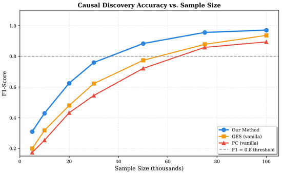
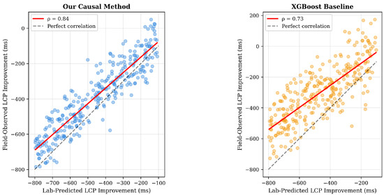
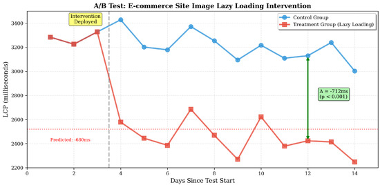
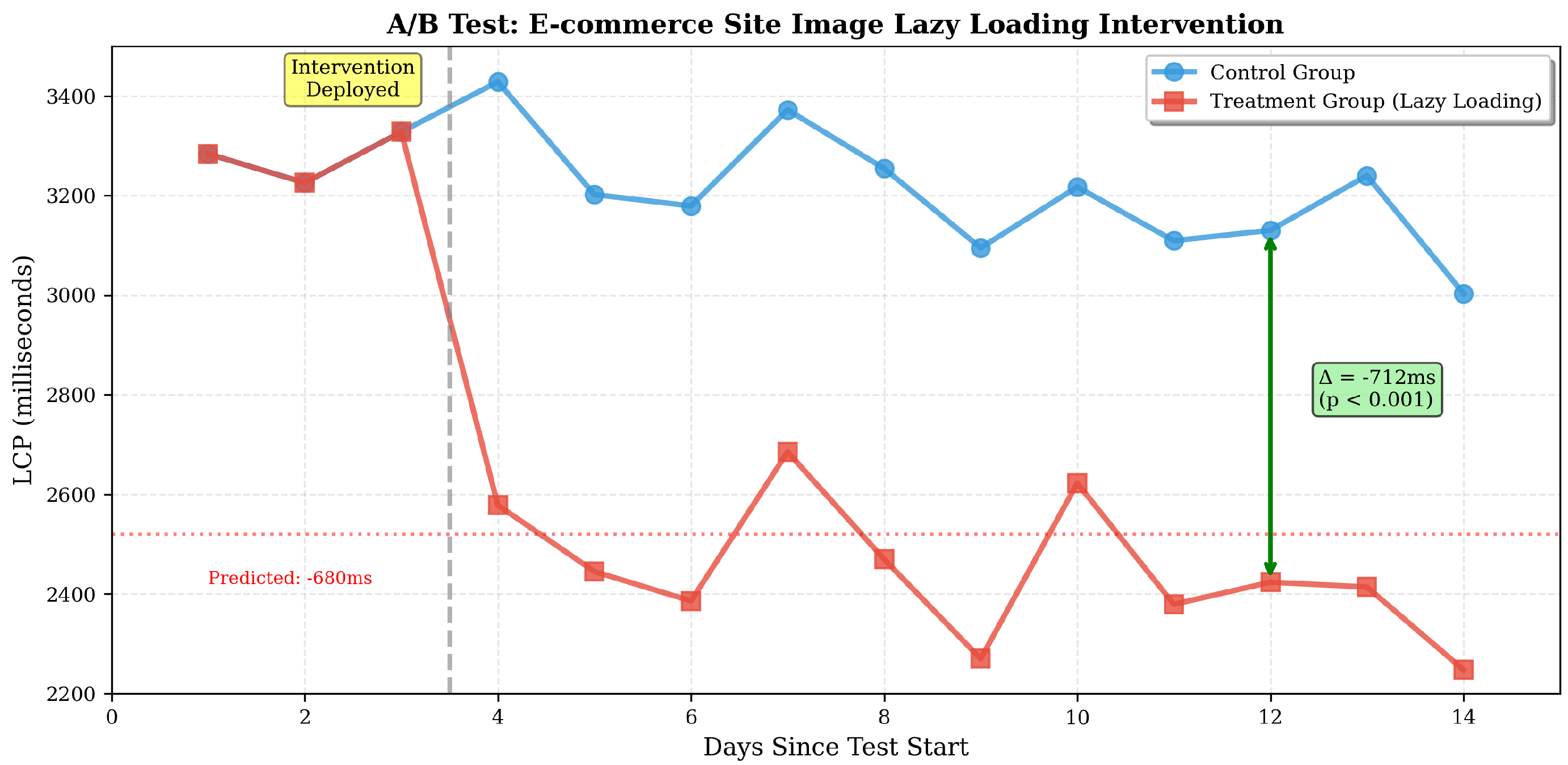
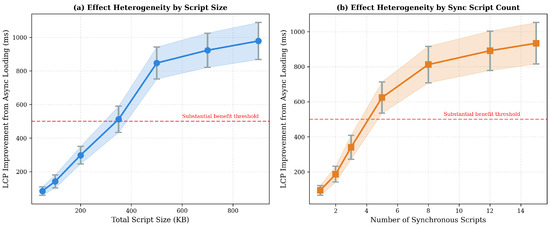
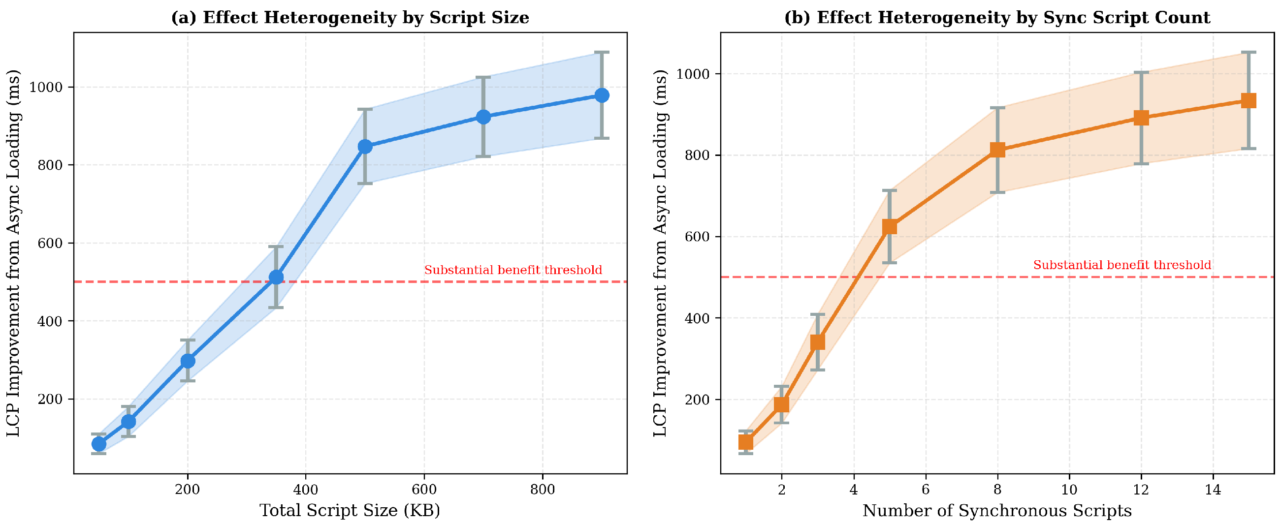
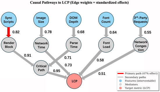
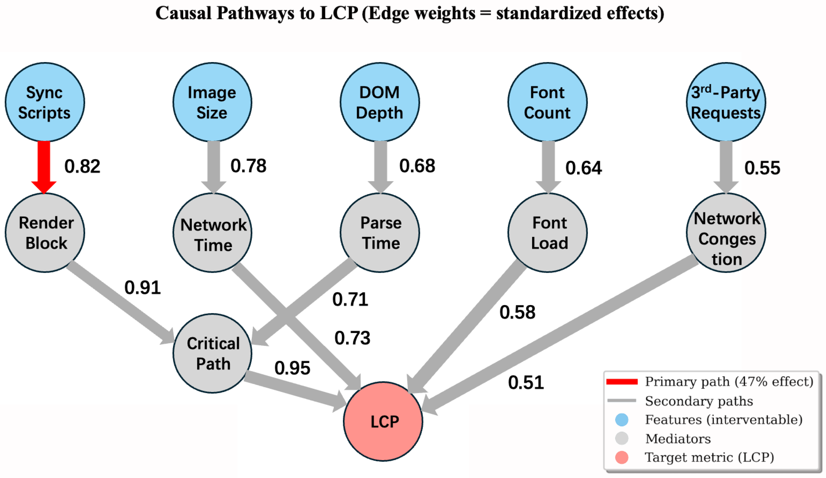
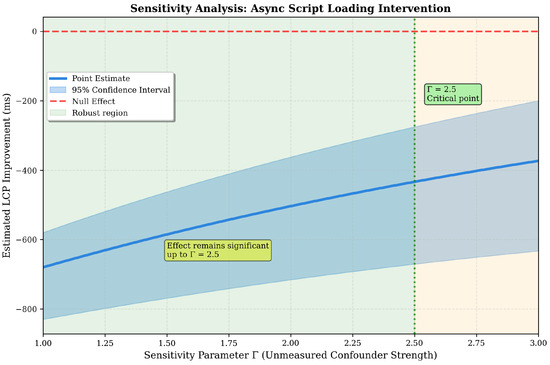
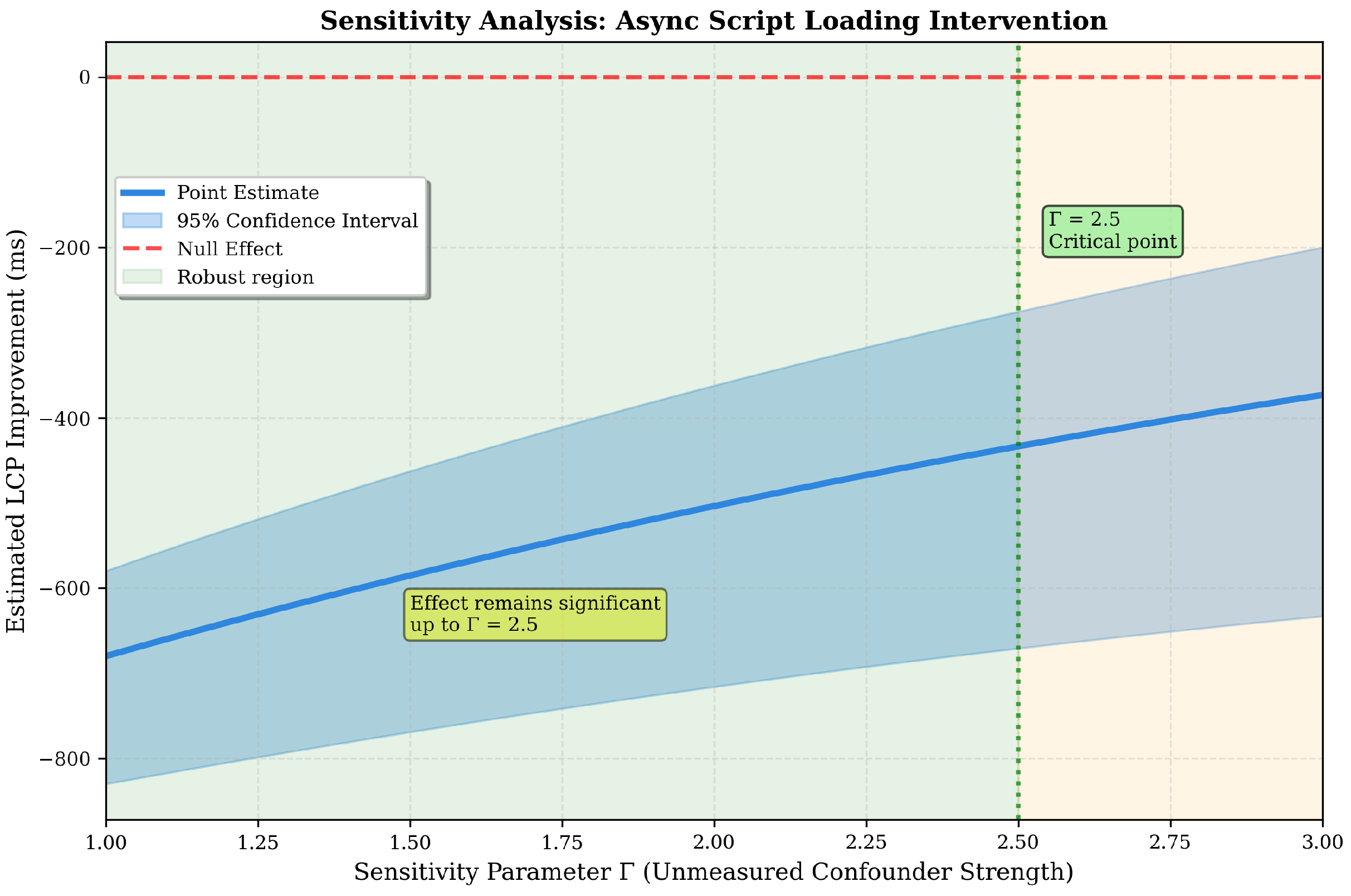
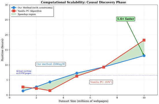
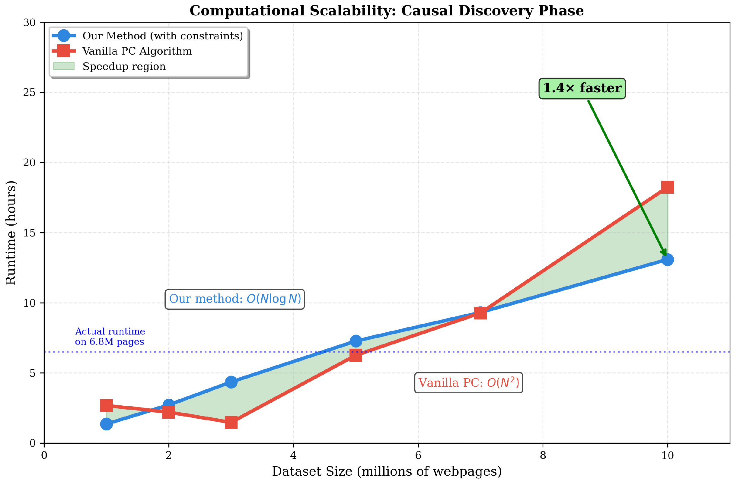

Disclaimer/Publisher’s Note: The statements, opinions and data contained in all publications are solely those of the individual author(s) and contributor(s) and not of MDPI and/or the editor(s). MDPI and/or the editor(s) disclaim responsibility for any injury to people or property resulting from any ideas, methods, instructions or products referred to in the content. |
© 2025 by the authors. Licensee MDPI, Basel, Switzerland. This article is an open access article distributed under the terms and conditions of the Creative Commons Attribution (CC BY) license (https://creativecommons.org/licenses/by/4.0/).