Study of Weak Solutions for a Class of Degenerate Parabolic Variational Inequalities with Variable Exponent

Abstract

The authors of this text study weak solutions to the variational inequalities with degenerate parabolic operators and symmetric structure in Sobolev spaces with variable exponent. The existence and uniqueness of the solutions are treated by using the penalty method and the reduction method in the weak sense. The authors also discuss the nonexistence and long-time behavior of solutions.

1. Introduction

Let $\Omega \subset {\mathrm{R}}_N$ be a bounded domain with appropriately smooth boundary $\partial \Omega$ and ${\Omega }_T=\Omega \times (0,T)$ be a cylinder of the height $T<\infty$. In this paper, we are concern with the following variational inequalities with degenerate parabolic operators:

$$min\left\{Lu,u-u_0\right\}=0,\mathrm{in}{\Omega }_T,$$

(1)

$$u(x,0)=u_0\left(x\right),\mathrm{in}\Omega ,$$

(2)

$$u(x,t)=0,\mathrm{on}\partial \Omega \times (0,T),\left(3\right)$$

(3)

where L are nonlinear degenerate parabolic operators, satisfying

$$Lu=u_t-u\mathrm{div}\left({\left|\nabla u\right|}^{p\left(x\right)-2}\nabla u\right)-\gamma {\left|\nabla u\right|}^{p\left(x\right)},$$

$p\left(x\right)$ is a measurable function. The problem (1)–(3) can be decomposed into two symmetric cases: if $Lu>0$, then $u=u_0\mathrm{in}{\Omega }_T.$ On the contrary, if $u>u_0$, $Lu=0\mathrm{in}{\Omega }_T.$

Many studies have been conducted on the questions of existence and uniqueness for variational inequalities with parabolic operators in the last three decades. Those works remain to be conducted on the case that L are linear parabolic operators (cf., e.g., [1,2,3,4,5,6,7]) defined by

$$Lu=\sum _{i=1}^n\frac{\partial }{\partial x_i}{a}_{ij}\left(x\right)\frac{\partial u}{\partial x_j}+\sum _{i=1}^n{b}_j\left(x\right)\frac{\partial u}{\partial x_j}+a_0\left(x\right)u.$$

where coefficients $a_{ij}\left(x\right)$, $b_i\left(x\right)$, $a_0\left(x\right)\in \overline{\Omega }$, $1\le i,j\le n$ are sufficiently smooth coefficients and satisfy the following conditions:

$$a_{ij}\left(x\right)=a_{ji}\left(x\right);a_0\left(x\right)\ge \beta >0,$$

$$\sum _{i,j=1}^n{a}_{ij}\left(x\right){\xi }_i{\xi }_j\ge \gamma {\left|\xi \right|}^2,\xi \in {\mathrm{R}}^{\mathrm{n}},\gamma >0,x\in \overline{\Omega },$$

where $\beta$ is a positive constant. The existence and uniqueness of this solution has been studied and established over the past years (see [1,3,4,7] for details).

To the best of our knowledge, there are only few works on the parabolic inequalities with degenerate operators. For example, the authors in [8] investigated a parabolic inequality where L is defined by

$$Lu=u_t-u\mathrm{div}\left({\left|\nabla u\right|}^{p-2}\nabla u\right)-\gamma {\left|\nabla u\right|}^p$$

whose coefficients p and $\gamma$ are positive constants. We use the penalty method and the reduction method to prove the existence of the solutions in the weak sense.

The present paper can be considered as a generalization of the results in [8]. We study the existence, uniqueness, and nonexistence of the parabolic variational inequalities without the restriction that $p\left(x\right)$ is a positive constant. To overcome the difficulties caused by $p\left(x\right)$, we introduce some novel ideas and techniques.

The paper is organized as follows: In Section 2, we introduce some generalized Lebesgue and Sobolev spaces and our main theorems. Section 3 analyses the existence and uniqueness of solutions to parabolic variational inequalities (1). Section 4 proves the nonexistence and long-time behavior of the solutions.

2. Basic Spaces and the Main Results

Denote

$p^{+}=\underset{\overline{\Omega }}{\mathrm{esssup}}p\left(x\right),p^{-}=\underset{\overline{\Omega }}{\mathrm{essinf}}p\left(x\right).$

In this paper we assume that

$$2<p^{-}\le p\left(x\right)\le p^{+}<\infty ,\forall x\in \Omega .$$

To study our problems, we need to introduce some new function spaces

$${\left|u\right|}_{L^{p\left(x\right)}(\Omega )}^{p\left(x\right)}=inf\left\{\left.\lambda \right|{\int }_{\Omega }\left|{\lambda }^{-1}u\left(x\right)\right|\mathrm{d}x\le 1\right\},$$

$$W^{1,p\left(x\right)}(\Omega )=\left\{u\in L^{p\left(x\right)}(\Omega )\left|\left|\nabla u\right|\in L^{p\left(x\right)}(\Omega )\right.\right\},$$

$${\left|u\right|}_{W^{1,p\left(x\right)}(\Omega )}={\left|u\right|}_{L^{p\left(x\right)}(\Omega )}+{\left|\nabla u\right|}_{L^{p\left(x\right)}(\Omega )},\forall u\in W^{1,p\left(x\right)}(\Omega ).$$

Here, we use $W_0^{1,p\left(x\right)}(\Omega )$ to denote the closure of $C_0^{\infty }$ in $W^{1,p\left(x\right)}(\Omega )$.

In the following parts, we state some properties of the function spaces introduced above (see [9,10]).

Proposition 1.

(i) The space $L^{p\left(x\right)}(\Omega )$, $W^{1,p\left(x\right)}(\Omega )$, and $W_0^{1,p\left(x\right)}(\Omega )$ are reflexive Banach spaces.

(ii) Let $q_1\left(x\right)$ and $q_2\left(x\right)$ be real functions with $1/\phantom{1q_1\left(x\right)}{q}_1\left(x\right)+1/\phantom{1q_2\left(x\right)}{q}_2\left(x\right)=1$ and $q_1\left(x\right)>1$. Then, the conjugate space of $L^{q_1\left(x\right)}(\Omega )$ is $L^{q_2\left(x\right)}(\Omega )$. For any $u\in L^{q_1\left(x\right)}(\Omega )$ and $v\in L^{q_2\left(x\right)}(\Omega )$, we have

$$\left|{\int }_{\Omega }uv\mathrm{d}x\right|\le 2{\left|u\right|}_{L^{q_1\left(x\right)}(\Omega )}{\left|v\right|}_{L^{q_2\left(x\right)}(\Omega )}.$$

(iii) if ${\left|u\right|}_{L^{p\left(x\right)}(\Omega )}=1$, then ${\int }_{\Omega }{\left|u\right|}^{p\left(x\right)}\mathrm{d}x=1$,

if ${\left|u\right|}_{L^{p\left(x\right)}(\Omega )}>1$, then ${\left|u\right|}_{L^{p\left(x\right)}(\Omega )}^{p^{-}}\le {\int }_{\Omega }{\left|u\right|}^{p\left(x\right)}\mathrm{d}x\le {\left|u\right|}_{L^{p\left(x\right)}(\Omega )}^{p^{+}}$,

if ${\left|u\right|}_{L^{p\left(x\right)}(\Omega )}<1$, then ${\left|u\right|}_{L^{p\left(x\right)}(\Omega )}^{p^{+}}\le {\int }_{\Omega }{\left|u\right|}^{p\left(x\right)}\mathrm{d}x\le {\left|u\right|}_{L^{p\left(x\right)}(\Omega )}^{p^{-}}$.

(iv) If $p_1\left(x\right)\le p_2\left(x\right)$, then $L^{p_1\left(x\right)}(\Omega )\supset L^{p_2\left(x\right)}(\Omega )$.

Proposition 2.

(i) If $p\left(x\right)\in C\left(\overline{\Omega }\right)$, then there is a constant $C>0$, such that

$${\left|u\right|}_{L^{p\left(x\right)}(\Omega )}^{}\le C{\left|\nabla u\right|}_{L^{p\left(x\right)}(\Omega )}^{},\forall u\in W_0^{1,p\left(x\right)}(\Omega ).$$

this implies that ${\left|\nabla u\right|}_{L^{p\left(x\right)}(\Omega )}$ and ${\left|u\right|}_{W^{1,p\left(x\right)}(\Omega )}$ are equivalent norms of $W_0^{1,p\left(x\right)}(\Omega )$.

Now, we give some lemmas, which are the main tools to prove Theorems 1–5 (see [10]).

Proposition 3.

Let $\theta \ge 0$ and $A\left(\eta \right)={({\eta }^2+\theta )}^{\frac{p\left(x\right)-2}{2}}\eta$. Then,

$$\left[A\left(\eta \right)-A\left({\eta }^{\prime }\right)\right]·\left[\eta -{\eta }^{\prime }\right]\ge C{\left|\eta -{\eta }^{\prime }\right|}^{p\left(x\right)},\forall \eta ,{\eta }^{\prime }\in \mathrm{R},$$

where C is a positive constant depending only on $p\left(x\right)$.

Proposition 4.

Assume that there exists $u_1$ and $u_2$, satisfying

$$L{u}_1\le L{u}_2\mathrm{for}\mathrm{all}(x,t)\in {\Omega }_T,$$

(4)

and $u_2\ge c$ in ${\Omega }_T$ for some $c>0$. If $u_2(x,0)\ge u_1(x,0)$ a.e in Ω, and $u_2(x,t)\ge u_1(x,t)$ a.e on $\partial \Omega \times (0,T)$, then $u_2(x,t)\ge u_1(x,t)$ in ${\Omega }_T$.

Proposition 5.

Assume $f(x,t,u)$ is nondecreasing in u for fixed $(x,t)$. If the condition (4) is replaced by

$$L{u}_1+f(x,t,u_1)\le L{u}_2+f(x,t,u_2)\mathrm{for}\mathrm{all}(x,t)\in {\Omega }_T,$$

the assertion of Proposition 4 remains true.

In spirit of [3,4], we introduce the following maximal monotone graph

$$G\left(\lambda \right)=\left\{\begin{array}{c}0,\lambda >0,\hfill \\ \left[0,1\right],\lambda =0.\hfill \end{array}\right.$$

in addition, we also define a function class for the solutions as follows:

$$B=\left\{u\in L^{\infty }\left({\Omega }_T\right)\cap L^{p\left(x\right)}(0,T;W_0^{1,p\left(x\right)}(\Omega ))\right\}.$$

based on the above basic knowledge, we define the weak solutions of problem (1) below.

Definition 1.

A pair $(u,\xi )\in B\times L^{\infty }\left({\Omega }_T\right)$ is called a weak solution of problem (1) if

(a) $u(x,t)\ge u_0\left(x\right)$, (b) $u(x,0)=u_0\left(x\right),$ (c) $\xi \in G(u-u_0)$,

(d) $\int {\int }_{{\Omega }_T}\left(-u{\phi }_t+u{\left|\nabla u\right|}^{p\left(x\right)-2}\nabla u\nabla \phi +(1-\gamma ){\left|\nabla u\right|}^{p\left(x\right)}\phi \right)\mathrm{d}x\mathrm{d}t=\int {\int }_{{\Omega }_T}\xi \varphi \mathrm{d}x\mathrm{d}t,\forall \phi \in C_0^{\infty }\left({\Omega }_T\right),$

(e) $\underset{t\to \infty }{lim}{\int }_{\Omega }\left|u^{\mu }(x,t)-u_0^{\mu }\left(x\right)\right|\mathrm{d}x=0$ holds for some $\mu >0$.

Then, we have the following results concerning the existence, nonexistence, and uniqueness of the weak solution of problem (1).

Theorem 1.

Under the assumption $\gamma \in (0,1)$, the problem (1) admits a unique weak solution u with $\frac{\partial u^{\mu }}{\partial t}\in L^2\left({\Omega }_T\right)$, where $\mu =\frac{\gamma -1}{2}+1.$

Theorem 2.

Assume $0<A:={\left|u_0\right|}_{L^{\frac{\gamma +3}{2}}(\Omega )}<\infty$. Then:

(a) If $\gamma >3,$ problem (1) has no weak solutions.

(b) If $0<\gamma \le 1,$ and if u is a weak solution of variational inequality (1), there exists $C>0$ and $\alpha >0$,

$${\left|u\left(t\right)\right|}_{L^{1+\mu }(\Omega )}\le C{\left(1-e^{-\alpha t}+e^{-\alpha t}{A}^{1-p^{+}}\right)}^{-\frac{1}{1+p^{+}}},0<t<T.$$

(5)

Theorem 3.

Assume $0<A:={\left|u_0\right|}_{L^1(\Omega )}<\infty$. Then, we have the following conclusion:

(a) If $\gamma >1,$ any weak solution u of vairiational inequality (1) does not satisfy $\frac{\partial u}{\partial t}\in L^2\left({\Omega }_T\right)$ for any $T\ge 1$ if A is large enough.

(b) If $0<\gamma \le 1,$ and u is a weak solution of vairiational inequality (1)–(3), we have

$${\left|u\left(t\right)\right|}_{L^1(\Omega )}\le C{\left(1-e^{-\alpha t}\right)}^{-\frac{1}{1+p^{+}}},0<t<T,$$

(6)

where C and α are positive constants independent of T.

Remark 1.

By combining Theorems 1 and 2, we can obtain the existence of global solutions.

3. Existence and Uniqueness of Solutions

To prove our main results, let us consider an approximation problem

$$L{u}_{\epsilon }+{\beta }_{\epsilon }(u_{\epsilon }-u_0)=0,\mathrm{in}{\Omega }_T,$$

(7)

with the Dirichlet boundary condition

$$u_{\epsilon }(x,0)=u_{0\epsilon }\left(x\right)=u_0\left(x\right)+\epsilon ,\mathrm{on}\Omega ,$$

(8)

and initial condition

$$u_{\epsilon }(x,t)=\epsilon ,\mathrm{on}\partial \Omega \times (0,T),$$

(9)

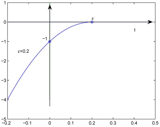
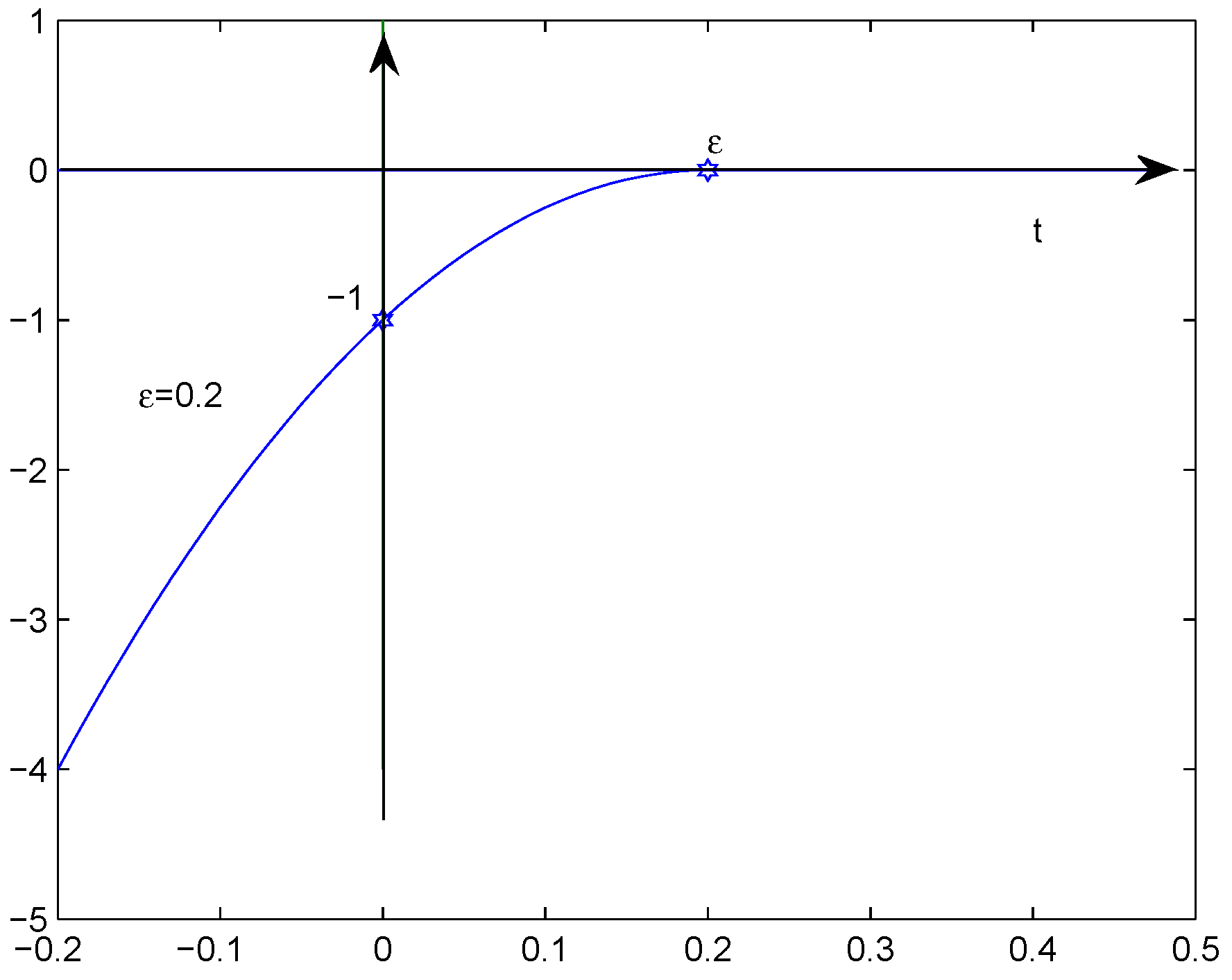
where the penalty function ${\beta }_{\epsilon }(·)$ is given by Figure 1, satisfying

$$\begin{array}{c}0<\epsilon \le 1,{\beta }_{\epsilon }\left(x\right)\in C^2\left(\mathrm{R}\right),{\beta }_{\epsilon }\left(x\right)\le 0,{{\beta }^{\prime }}_{\epsilon }\left(x\right)\ge 0,{{\beta }^{″}}_{\epsilon }\left(x\right)\le 0,\\ {\beta }_{\epsilon }\left(x\right)=\left\{\begin{array}{c}0,x\ge \epsilon ,\hfill \\ -1,x=0,\hfill \end{array}\right.\underset{\epsilon \to 0}{lim}{\beta }_{\epsilon }\left(x\right)=\left\{\begin{array}{c}0,x>0,\hfill \\ -\infty ,x<0.\hfill \end{array}\right.\end{array}$$

(10)

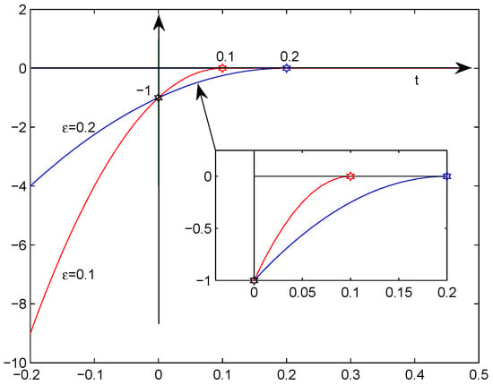
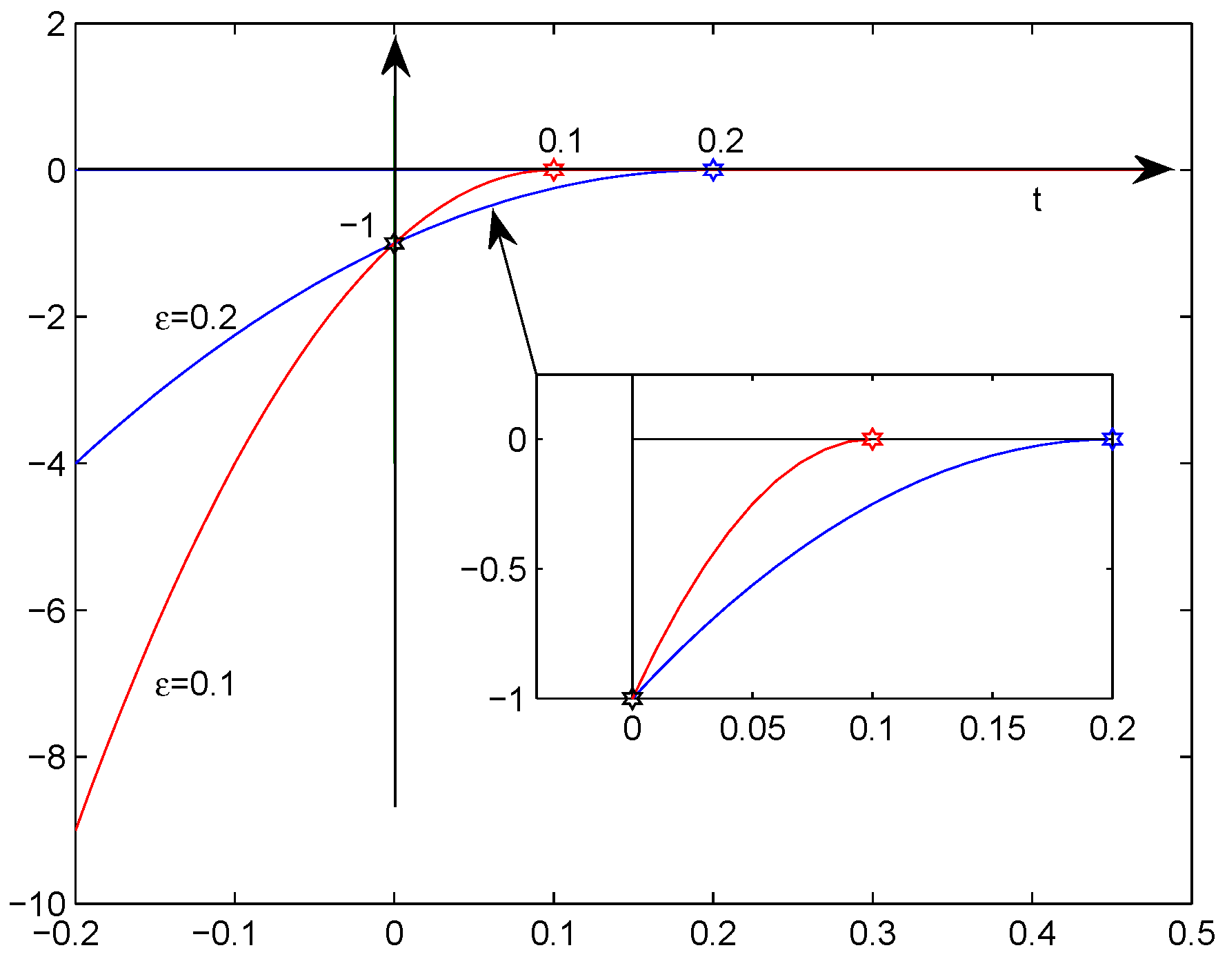
from Figure 2, we see that if ${\epsilon }_1\le {\epsilon }_2$, for all $t\in [0,\epsilon ]$,

$${\beta }_{{\epsilon }_1}\left(t\right)-{\beta }_{{\epsilon }_2}\left(t\right)\ge 0.$$

(11)

Figure 1. The penalty function ${\beta }_{0.2}$.

Figure 2. The penalty functions ${\beta }_{0.1}$ and ${\beta }_{0.2}$.

Applying the definition of ${\beta }_{\epsilon }(·)$, it is easy to find that

$$L{u}_{\epsilon }=0\iff u_{\epsilon }\ge u_0+\epsilon ,L{u}_{\epsilon }>0\iff u_{\epsilon }<u_0+\epsilon .$$

(12)

thus, we use ${\beta }_{\epsilon }(·)$ to control the inequalities. At the same time, we also use $\epsilon$ to regularize the initial-boundary value.

Definition 2.

A non-negative function $u_{\epsilon }$ is called a weak solution of problem (7)–(9), if

(a) $u_{\epsilon }\in L^{\infty }\left({\Omega }_T\right)\cap L^{p\left(x\right)}(0,T;W_0^{1,p\left(x\right)}(\Omega )),$

(b) for all $\phi \in C_0^{\infty }\left({\Omega }_T\right)$,

$$\int {\int }_{{\Omega }_T}\left(u_{\epsilon }{\phi }_t+u_{\epsilon }{\left|\nabla u_{\epsilon }\right|}^{p\left(x\right)-2}\nabla u_{\epsilon }\nabla \phi +(1-\gamma ){\left|\nabla u_{\epsilon }\right|}^{p\left(x\right)}\phi +{\beta }_{\epsilon }(u_{\epsilon }-u_0)\phi \right)\mathrm{d}x\mathrm{d}t=0,$$

(c) $\underset{t\to \infty }{lim}{\int }_{\Omega }\left|u_{\epsilon }^{\mu }(x,t)-u_{0\epsilon }^{\mu }\left(x\right)\right|\mathrm{d}x=0$ holds for some $\mu >0$.

It is known (see [9,10]) that when employing the difference scheme, there exists a weak solution $u_{\epsilon }$ to the nonlinear PDE (7)–(9) in the sense of Definition 2.

Lemma 1.

Let $\epsilon ,{\epsilon }_1$, and ${\epsilon }_2$ be positive constants satisfying $\epsilon \in (0,1)$, $0<{\epsilon }_1\le {\epsilon }_2<1$. Then

$$u_0\le u_{\epsilon }\le {\left|u_0\right|}_{\infty }+\epsilon ,$$

(13)

$$u_{{\epsilon }_1}(x,t)\le u_{{\epsilon }_2}(x,t)\mathrm{for}\mathrm{all}(x,t)\in {\Omega }_T.$$

(14)

Proof. 

First, we prove $u_{\epsilon }\ge u_0$. Letting $t=0$ in (7), we have

$${\partial }_t{u}_{0\epsilon }-L{u}_{0\epsilon }+{\beta }_{\epsilon }(u_{0\epsilon }-u_0)=0.$$

it follows the definition of ${\beta }_{\epsilon }(·)$ that

$${\beta }_{\epsilon }(u_{0\epsilon }-u_0)={\beta }_{\epsilon }\left(\epsilon \right)=0.$$

this leads to

$$L{u}_0=L{u}_{0\epsilon }=0,\forall x\in \Omega .$$

from (7) and (10), we obtain

$$L{u}_{\epsilon }=-{\beta }_{\epsilon }(u_{\epsilon }-u_0)\ge 0,\forall (x,t)\in {\Omega }_T.$$

Applying Proposition 4, and combining initial conditions (9) and boundary conditions (8), we have

$$u_{\epsilon }\ge u_{0\epsilon },\forall (x,t)\in {\Omega }_T.$$

Second, we consider $u(x,t)\le {\left|u_0\right|}_{\infty }+\epsilon$. Note that ${\left|u_0\right|}_{\infty }+\epsilon$ is a positive constant satisfying

$$u_{\epsilon }(x,t)\le {\left|u_0\right|}_{\infty }+\epsilon \mathrm{on}\partial \Omega \times (0,T)\mathrm{and}{u}_{0\epsilon }\left(x\right)\le {\left|u_0\right|}_{\infty }+\epsilon \mathrm{in}\Omega .$$

letting $t\to 0$ in (7), and applying the definition of ${\beta }_{\epsilon }(·)$, we have

$$L\left({\left|u_0\right|}_{\infty }+\epsilon \right)+{\beta }_{\epsilon }({\left|u_0\right|}_{\infty }+\epsilon -u_0)\ge {\beta }_{\epsilon }\left(\epsilon \right)=0.$$

(15)

thus, combining (7) and (15) and applying Proposition 4,

$$u_{\epsilon }(x,t)\le {\left|u_0\right|}_{\infty }+\epsilon \mathrm{in}\Omega \times (0,T).$$

Third, we aim to prove (14). From (7), we have

$$L{u}_{{\epsilon }_1}+{\beta }_{{\epsilon }_1}(u_{{\epsilon }_1}-u_0)=0,$$

$$L{u}_{{\epsilon }_2}+{\beta }_{{\epsilon }_2}(u_{{\epsilon }_2}-u_0)=0.$$

using (11) and the definition of ${\beta }_{\epsilon }(·)$ that

$$\begin{array}{c}L{u}_{{\epsilon }_2}+{\beta }_{{\epsilon }_1}(u_{{\epsilon }_2}-u_0)={\beta }_{{\epsilon }_1}(u_{{\epsilon }_2}-u_0)-{\beta }_{{\epsilon }_2}(u_{{\epsilon }_2}-u_0)\ge 0.\hfill \end{array}$$

thus, combining initial conditions (9) and boundary conditions (8), (14) can be proved by Proposition 5. □

Lemma 2.

For all $\alpha \in [0,1-\gamma )$, the solution of nonlinear PDE (7)–(9) satisfies

$${\left|\frac{\partial u_{\epsilon }^{\mu }}{\partial t}\right|}_{L^2\left({\Omega }_T\right)}+{\left|\frac{\partial u_{\epsilon }}{\partial t}\right|}_{L^2\left({\Omega }_T\right)}\le C,$$

(16)

$${\left|{\left|\nabla u_{\epsilon }\right|}^{p\left(x\right)}{u}_{\epsilon }^{-\alpha }\right|}_{L^1\left({\Omega }_T\right)}+{\left|\nabla u_{\epsilon }\right|}_{L^{p\left(x\right)}\left({\Omega }_T\right)}\le C,$$

(17)

where C is a positive constant independent of ε.

Proof. 

First, we prove (16). Multiplying (7) by $u_{\epsilon }^{\gamma -1}{\partial }_t{u}_{\epsilon }$, integrating both sides of equality over ${\Omega }_T$, and integrating by parts, we derive

$$\begin{array}{c}{\mu }^{-2}\int {\int }_{{\Omega }_T}{\left(\frac{\partial u_{\epsilon }^{\mu }}{\partial t}\right)}^2\mathrm{d}x\mathrm{d}t=\int {\int }_{{\Omega }_T}\left({\partial }_t{u}_{\epsilon }\right)u_{\epsilon }^{\gamma -1}{\partial }_t{u}_{\epsilon }\mathrm{d}x\mathrm{d}t\hfill \\ =-\int {\int }_{{\Omega }_T}{\left({\left|\nabla u_{\epsilon }\right|}^2\right)}^{\left(p\right(x)-2)/\phantom{\left(p\right(x)-2)2}2}\nabla u_{\epsilon }\nabla (u_{\epsilon }^{\gamma }{\partial }_t{u}_{\epsilon })\mathrm{d}x\mathrm{d}t\hfill \\ +\gamma \int {\int }_{{\Omega }_T}{\left({\left|\nabla u_{\epsilon }\right|}^2\right)}^{p\left(x\right)/\phantom{p\left(x\right)2}2}{u}_{\epsilon }^{\gamma -1}{\partial }_t{u}_{\epsilon }\mathrm{d}x\mathrm{d}t-\int {\int }_{{\Omega }_T}{\beta }_{\epsilon }(u_{\epsilon }-u_0)u_{\epsilon }^{\gamma }{\partial }_t{u}_{\epsilon }\mathrm{d}x\mathrm{d}t\hfill \\ \le -\int {\int }_{{\Omega }_T}{u}_{\epsilon }^{\gamma }{\left({\left|\nabla u_{\epsilon }\right|}^2\right)}^{\left(p\right(x)-2)/\phantom{\left(p\right(x)-2)2}2}\nabla u_{\epsilon }\nabla ({\partial }_t{u}_{\epsilon })\mathrm{d}x\mathrm{d}t+{({\left|u_0\right|}_{\infty }+1)}^{\gamma }{\int }_{\Omega }\left|{\int }_0^T{\partial }_t{u}_{\epsilon }\mathrm{d}t\right|\mathrm{d}x\hfill \\ \le -\int {\int }_{{\Omega }_T}{u}_{\epsilon }^{\gamma }p{\left(x\right)}^{-1}{\partial }_t{\left({\left|\nabla u_{\epsilon }\right|}^2\right)}^{p\left(x\right)/\phantom{p\left(x\right)2}2}\mathrm{d}x\mathrm{d}t+2{({\left|u_0\right|}_{\infty }+1)}^{\gamma +1}.\hfill \end{array}$$

applying Proposition 1(iii) and Lemma 1, we obtain

$$\begin{array}{c}{\mu }^{-2}\int {\int }_{{\Omega }_T}{\left(\frac{\partial u_{\epsilon }^{\mu }}{\partial t}\right)}^2\mathrm{d}x\mathrm{d}t\hfill \\ \le \frac{1}{p^{-}}{({\left|u_0\right|}_{\infty }+1)}^{\gamma }\left({\left|\nabla u_0\right|}_{L^{p\left(x\right)}\left({\Omega }_T\right)}^{p^{-}/\phantom{p^{-}{p}^{+}}{p}^{+}}+{\left|\nabla u_0\right|}_{L^{p\left(x\right)}\left({\Omega }_T\right)}^{p^{+}/\phantom{p^{+}{p}^{-}}{p}^{-}}\right)+2{({\left|u_0\right|}_{\infty }+1)}^{\gamma +1}.\hfill \end{array}$$

(18)

note that $\gamma \in (0,1),2(\mu -1)=\gamma -1.$ Using Lemma 1, we derive

$$\begin{array}{c}\int {\int }_{{\Omega }_T}{\left(\frac{\partial u_{\epsilon }}{\partial t}\right)}^2\mathrm{d}x\mathrm{d}t=\int {\int }_{{\Omega }_T}{\left(\frac{\partial u_{\epsilon }^{\mu }}{\partial t}\right)}^2{u}_{\epsilon }^{\frac{1}{\gamma -1}}\mathrm{d}x\mathrm{d}t\hfill \\ \le {({\left|u_0\right|}_{\infty }+1)}^{\frac{1}{\gamma -1}}\int {\int }_{{\Omega }_T}{\left(\frac{\partial u_{\epsilon }^{\mu }}{\partial t}\right)}^2\mathrm{d}x\mathrm{d}t.\hfill \end{array}$$

(19)

combining (18) and (19), (16) is proved.

Second we prove (17). Multiply (9) by $u_{\epsilon }^{-\alpha }$ and integrate both sides of the equation over ${\Omega }_T$. After integrating by parts, we obtain

$$\begin{array}{c}\int {\int }_{{\Omega }_T}\frac{\partial u_{\epsilon }}{\partial t}{u}_{\epsilon }^{-\alpha }\mathrm{d}x\mathrm{d}t\hfill \\ =\int {\int }_{{\Omega }_T}{u}_{\epsilon }^{1-\alpha }\mathrm{div}\left\{{\left|\nabla u_{\epsilon }\right|}^{p\left(x\right)-2}\nabla u_{\epsilon }\right\}+\gamma u_{\epsilon }^{-\alpha }{\left|\nabla u_{\epsilon }\right|}^{p\left(x\right)}-u_{\epsilon }^{-\alpha }{\beta }_{\epsilon }(u_{\epsilon }-u_0)\mathrm{d}x\mathrm{d}t\hfill \\ ={\int }_0^T{\int }_{\partial \Omega }\left\{u_{\epsilon }^{1-\alpha }{\left|\nabla u_{\epsilon }\right|}^{p\left(x\right)-2}\frac{\partial u_{\epsilon }}{\partial \nu }\right\}\mathrm{d}x\mathrm{d}t-(1-\alpha -\gamma )\int {\int }_{{\Omega }_T}{u}_{\epsilon }^{-\alpha }{\left|\nabla u_{\epsilon }\right|}^{p\left(x\right)}\mathrm{d}x\mathrm{d}t\hfill \\ -\int {\int }_{{\Omega }_T}{u}_{\epsilon }^{-\alpha }{\beta }_{\epsilon }\left(u_{\epsilon }-u_0\right)\mathrm{d}x\mathrm{d}t,\hfill \end{array}$$

(20)

where $\nu$ denotes the outward normal to $\partial \Omega \times (0,T)$. Furthermore, putting together (10) and (13) implies

$$\int {\int }_{{\Omega }_T}{u}_{\epsilon }^{-\alpha }{\beta }_{\epsilon }\left(u_{\epsilon }-u_0\right)\mathrm{d}x\mathrm{d}t\le 0.$$

(21)

since $u_{\epsilon }\ge \epsilon$, we have

$$\frac{\partial u_{\epsilon }}{\partial \nu }\le 0\mathrm{on}\partial \Omega \times (0,T).$$

this leads to

$${\int }_0^T{\int }_{\partial \Omega }\left\{u_{\epsilon }^{1-\alpha }{\left|\nabla u_{\epsilon }\right|}^{p\left(x\right)-2}\frac{\partial u_{\epsilon }}{\partial \nu }\right\}\mathrm{d}x\mathrm{d}t\le 0.$$

(22)

now, we drop the nonpositive term (21) and (22) in (20) to obtain

$$\int {\int }_{{\Omega }_T}\frac{\partial u_{\epsilon }}{\partial t}{u}_{\epsilon }^{-\alpha }\mathrm{d}x\mathrm{d}t\le -(1-\alpha -\gamma )\int {\int }_{{\Omega }_T}{u}_{\epsilon }^{-\alpha }{\left|\nabla u_{\epsilon }\right|}^{p\left(x\right)}\mathrm{d}x\mathrm{d}t.$$

(23)

clearly, using integration by parts, we derive

$$\int {\int }_{{\Omega }_T}\frac{\partial u_{\epsilon }}{\partial t}{u}_{\epsilon }^{-\alpha }\mathrm{d}x\mathrm{d}t=\frac{1}{1-\alpha }{\int }_{\Omega }{u}_{\epsilon }^{1-\alpha }(x,T)-u_{\epsilon }^{1-\alpha }(x,0)\mathrm{d}x.$$

this and (23) lead to

$$\int {\int }_{{\Omega }_T}{\left|\nabla u_{\epsilon }\right|}^{p\left(x\right)}{u}_{\epsilon }^{-\alpha }\mathrm{d}x\mathrm{d}t\le \frac{1}{(1-\alpha -\gamma )(1-\alpha )}{\int }_{\Omega }{u}_{\epsilon }^{-\alpha }(x,0)\mathrm{d}x\le C.$$

where $C>0$ depend on $\alpha ,\gamma ,\Omega$, and ${\left|u_0\right|}_{\infty }$. Hence, the proof is completed. □

Lemmas 1 and 2 imply that, for any $\epsilon \in (0,1)$, there exists a subsequence of $\left\{u_{\epsilon }\right\}$, still denoted by $\left\{u_{\epsilon }\right\}$, and a function u with $u\in L^{\infty }\left({\Omega }_T\right)$, such that, as $\epsilon \to 0$

$$u_{\epsilon }\to u\mathrm{a}.\mathrm{e}.\mathrm{in}{\Omega }_T,$$

(24)

$$\nabla u_{\epsilon }\stackrel{w}{\to }\nabla u\mathrm{in}{L}^{p\left(x\right)}\left({\Omega }_T\right),$$

(25)

$$\frac{\partial u_{\epsilon }}{\partial t}\stackrel{w}{\to }\frac{\partial u}{\partial t}\mathrm{in}{L}^2\left({\Omega }_T\right),$$

(26)

where $\stackrel{w}{\to }$ denotes weak convergence, and

$$u_0\le u\le \left|u_0\right|,u\le u_{\epsilon }\mathrm{a}.\mathrm{e}.\mathrm{in}{\Omega }_T.$$

(27)

Lemma 3.

Assume $Q_c^{\epsilon }=\left\{(x,t)\in {\Omega }_T;u_{\epsilon }\ge c,c>0\right\}$, $Q_c^{}=\left\{(x,t)\in {\Omega }_T;u\ge c,c>0\right\}$, and let $0<c<1$. Then, $\nabla u_{\epsilon }$ converge to $\nabla u$ in norm $L^{p\left(x\right)}$, such that as $\epsilon \to 0$,

$${\left|\nabla u_{\epsilon }-\nabla u\right|}_{L^{p\left(x\right)}\left({\Omega }_T\right)}\to 0,$$

(28)

$${\left|\nabla u_{\epsilon }-\nabla u\right|}_{L^{p\left(x\right)}\left(Q_c^{\epsilon }\right)}\to 0,$$

(29)

$${\left|\nabla u_{\epsilon }-\nabla u\right|}_{L^{p\left(x\right)}\left(Q_c\right)}\to 0.$$

(30)

Proof .

Choosing $\phi =u_{\epsilon }^{p^{-}-2}(u_{\epsilon }^2-{\epsilon }^2-u^2)$ as the test function in

$$\int {\int }_{{\Omega }_T}\left(u_{\epsilon }{\phi }_t+u_{\epsilon }{\left|\nabla u_{\epsilon }\right|}^{p\left(x\right)-2}\nabla u_{\epsilon }\nabla \phi +(1-\gamma ){\left|\nabla u_{\epsilon }\right|}^{p\left(x\right)}\phi -{\beta }_{\epsilon }(u_{\epsilon }-u_0)\phi \right)\mathrm{d}x\mathrm{d}t=0,$$

it is easy to see that

$$\begin{array}{c}\int {\int }_{{\Omega }_T}\frac{\partial u_{\epsilon }}{\partial t}{u}_{\epsilon }^{p^{-}-2}(u_{\epsilon }^2-{\epsilon }^2-u^2)\mathrm{d}x\mathrm{d}t\hfill \\ =-\int {\int }_{{\Omega }_T}{\left|\nabla u_{\epsilon }\right|}^{p\left(x\right)-2}\nabla u_{\epsilon }\nabla \left\{u_{\epsilon }^{p^{-}-1}(u_{\epsilon }^2-{\epsilon }^2-u^2)\right\}\mathrm{d}x\mathrm{d}t\hfill \\ +\gamma \int {\int }_{{\Omega }_T}{u}_{\epsilon }^{p^{-}-2}{\left|\nabla u_{\epsilon }\right|}^{p\left(x\right)}(u_{\epsilon }^2-{\epsilon }^2-u^2)\mathrm{d}x\mathrm{d}t\hfill \\ +{\int }_{{\Omega }_T}{u}_{\epsilon }^{p^{-}-2}(u_{\epsilon }^2-{\epsilon }^2-u^2){\beta }_{\epsilon }(u_{\epsilon }-u_0)\mathrm{d}x\mathrm{d}t\hfill \\ =-\int {\int }_{{\Omega }_T}{u}_{\epsilon }^{p^{-}-1}{\left|\nabla u_{\epsilon }\right|}^{p\left(x\right)-2}\nabla u_{\epsilon }\nabla (u_{\epsilon }^2-u^2)\mathrm{d}x\mathrm{d}t\hfill \\ +\int {\int }_{{\Omega }_T}{u}_{\epsilon }^{p^{-}-2}(u_{\epsilon }^2-{\epsilon }^2-u^2){\beta }_{\epsilon }(u_{\epsilon }-u_0)\mathrm{d}x\mathrm{d}t\hfill \\ +(\gamma -p^{-}+1)\int {\int }_{{\Omega }_T}{u}_{\epsilon }^{p^{-}-2}{\left|\nabla u_{\epsilon }\right|}^{p\left(x\right)}(u_{\epsilon }^2-{\epsilon }^2-u^2)\mathrm{d}x\mathrm{d}t.\hfill \end{array}$$

(31)

from (27) and the definition of ${\beta }_{\epsilon }$, we derive

$${\int }_{{\Omega }_T}{u}_{\epsilon }^{p^{-}-2}{\left|\nabla u_{\epsilon }\right|}^{p\left(x\right)}(u_{\epsilon }^2-{\epsilon }^2-u^2)\mathrm{d}x\mathrm{d}t\ge -{\epsilon }^2{\int }_{{\Omega }_T}{u}_{\epsilon }^{p^{-}-2}{\left|\nabla u_{\epsilon }\right|}^{p\left(x\right)}\mathrm{d}x\mathrm{d}t,$$

(32)

$$\begin{array}{c}{\int }_{{\Omega }_T}{u}_{\epsilon }^{p^{-}-2}(u_{\epsilon }^2-{\epsilon }^2-u^2){\beta }_{\epsilon }(u_{\epsilon }-u_0)\mathrm{d}x\mathrm{d}t\hfill \\ \le {\left({\left|u_0\right|}_{\infty }+\epsilon \right)}^{p^{-}-2}\left|{\int }_{{\Omega }_T}(u_{\epsilon }^2-{\epsilon }^2-u^2)\mathrm{d}x\mathrm{d}t\right|.\hfill \end{array}$$

(33)

observing that $\gamma -p^{-}+1<0$, and combing (31), (32), and (33), we have

$$\begin{array}{c}{\int }_{{\Omega }_T}\frac{\partial u_{\epsilon }}{\partial t}{u}_{\epsilon }^{p^{-}-2}(u_{\epsilon }^2-{\epsilon }^2-u^2)\mathrm{d}x\mathrm{d}t\hfill \\ \le -2^{1-p^{-}}{\int }_{{\Omega }_T}{\left|\nabla u_{\epsilon }^2\right|}^{p\left(x\right)-2}\nabla u_{\epsilon }^2\nabla (u_{\epsilon }^2-u^2)\mathrm{d}x\mathrm{d}t\hfill \\ +p^{-}{\epsilon }^2{\int }_{{\Omega }_T}{u}_{\epsilon }^{p^{-}-2}{\left|\nabla u_{\epsilon }\right|}^{p\left(x\right)}\mathrm{d}x\mathrm{d}t\hfill \\ +{\left({\left|u_0\right|}_{\infty }+\epsilon \right)}^{p^{-}-2}\left|{\int }_{{\Omega }_T}(u_{\epsilon }^2-{\epsilon }^2-u^2)\mathrm{d}x\mathrm{d}t\right|.\hfill \end{array}$$

note that $\epsilon \le u_{\epsilon }\le {\left|u_0\right|}_{\infty }+\epsilon$. Thus, it follows by the trigonometrical inequality that

$$\begin{array}{c}{\int }_{{\Omega }_T}\frac{\partial u_{\epsilon }}{\partial t}{u}_{\epsilon }^{p^{-}-2}(u_{\epsilon }^2-{\epsilon }^2-u^2)\mathrm{d}x\mathrm{d}t\hfill \\ +{\int }_{{\Omega }_T}\left[{\left|\nabla u_{\epsilon }^2\right|}^{p\left(x\right)-2}\nabla u_{\epsilon }^2-{\left|\nabla u_{}^2\right|}^{p\left(x\right)-2}\nabla u_{}^2\right]\nabla (u_{\epsilon }^2-u^2)\mathrm{d}x\mathrm{d}t\hfill \\ \le -2^{1-p^{-}}{\int }_{{\Omega }_T}{\left|\nabla u_{}^2\right|}^{p\left(x\right)-2}\nabla u_{}^2\nabla (u_{\epsilon }^2-u^2)\mathrm{d}x\mathrm{d}t\hfill \\ +p^{-}{\epsilon }^2{\int }_{{\Omega }_T}{u}_{\epsilon }^{p^{-}-2}{\left|\nabla u_{\epsilon }\right|}^{p\left(x\right)}\mathrm{d}x\mathrm{d}t\hfill \\ +{\left({\left|u_0\right|}_{\infty }+\epsilon \right)}^{p^{-}-2}\left|{\int }_{{\Omega }_T}(u_{\epsilon }^2-{\epsilon }^2-u^2)\mathrm{d}x\mathrm{d}t\right|.\hfill \end{array}$$

(34)

from (13) and (16), using Holder inequality derives

$${\int }_{{\Omega }_T}{\left(\frac{\partial u_{\epsilon }^{p^{-}-1}}{\partial t}\right)}^2\mathrm{d}x\mathrm{d}t\le {(p^{-}-1)}^2{({\left|u_0\right|}_{\infty }+1)}^{p^{-}-2}{\left|\frac{\partial u_{\epsilon }}{\partial t}\right|}_{L^2\left({\Omega }_T\right)}^2<\infty .$$

(35)

this leads to

$$\begin{array}{c}\left|{\int }_{{\Omega }_T}\frac{\partial u_{\epsilon }}{\partial t}{u}_{\epsilon }^{p^{-}-2}(u_{\epsilon }^2-{\epsilon }^2-u^2)\mathrm{d}x\mathrm{d}t\right|\hfill \\ \le \frac{1}{p^{-}-1}{\int }_{{\Omega }_T}\left|\frac{\partial u_{\epsilon }^{p^{-}-1}}{\partial t}(u_{\epsilon }^2-{\epsilon }^2-u^2)\right|\mathrm{d}x\mathrm{d}t\hfill \\ \le \frac{1}{p^{-}-1}\sqrt{{\int }_{{\Omega }_T}{\left(\frac{\partial u_{\epsilon }^{p^{-}-1}}{\partial t}\right)}^2\mathrm{d}x\mathrm{d}t}·\sqrt{{\int }_{{\Omega }_T}{(u_{\epsilon }^2-{\epsilon }^2-u^2)}^2\mathrm{d}x\mathrm{d}t}\hfill \\ \le \frac{1}{p^{-}-1}{\epsilon }^2\sqrt{\left|{\Omega }_T\right|}\sqrt{{\int }_{{\Omega }_T}{\left(\frac{\partial u_{\epsilon }^{p^{-}-1}}{\partial t}\right)}^2\mathrm{d}x\mathrm{d}t}\to 0,\epsilon \to 0.\hfill \end{array}$$

(36)

moreover, (24) and (25) imply that as $\epsilon \to 0$,

$${\left({\left|u_0\right|}_{\infty }+\epsilon \right)}^{p^{-}-2}\left|{\int }_{{\Omega }_T}(u_{\epsilon }^2-{\epsilon }^2-u^2)\mathrm{d}x\mathrm{d}t\right|\to 0,$$

(37)

$$\nabla u_{\epsilon }^2\stackrel{w}{\to }\nabla u_{}^2\mathrm{in}{L}^{p\left(x\right)}\left({\Omega }_T\right).$$

(38)

substituting (36)–(38) into (34), we have

$$\underset{\epsilon \to 0}{limsup}{\int }_{{\Omega }_T}\left[{\left|\nabla u_{\epsilon }^2\right|}^{p\left(x\right)-2}\nabla u_{\epsilon }^2-{\left|\nabla u_{}^2\right|}^{p\left(x\right)-2}\nabla u_{}^2\right]\nabla (u_{\epsilon }^2-u^2)\mathrm{d}x\mathrm{d}t\le 0.$$

this and Proposition 3 lead to

$$\underset{\epsilon \to 0}{lim}{\int }_{{\Omega }_T}{\left|\nabla u_{\epsilon }^2-\nabla u_{}^2\right|}^{p\left(x\right)}\mathrm{d}x\mathrm{d}t=0.$$

(39)

hence, in view of

$$\nabla u_{\epsilon }^2-\nabla u^2=2u_{\epsilon }\nabla u_{\epsilon }-2u\nabla u=2u_{\epsilon }(\nabla u_{\epsilon }-\nabla u)+2\nabla u\left(u_{\epsilon }-u\right),$$

$$\nabla u_{\epsilon }^2-\nabla u^2=2u_{\epsilon }\nabla u_{\epsilon }-2u\nabla u=2u(\nabla u_{\epsilon }-\nabla u)+2\nabla u_{\epsilon }(u_{\epsilon }-u),$$

we have that as $\epsilon \to 0$,

$$\begin{array}{c}{2}^{p^{-}}{\int }_{{\Omega }_T}{u}_{\epsilon }^{p\left(x\right)}{\left|\nabla u_{\epsilon }-\nabla u\right|}^{p\left(x\right)}\mathrm{d}x\mathrm{d}t\hfill \\ \le 2^{p^{+}}{\int }_{{\Omega }_T}{\left|\nabla u_{\epsilon }^2-\nabla u^2\right|}^{p\left(x\right)}\mathrm{d}x\mathrm{d}t+4^{p^{+}}{\int }_{{\Omega }_T}{\left|\nabla u\right|}^{p\left(x\right)}{\left|u_{\epsilon }-u\right|}^{p\left(x\right)}\mathrm{d}x\mathrm{d}t\to 0,\hfill \end{array}$$

$$\begin{array}{c}{2}^{p^{-}}{\int }_{{\Omega }_T}{u}^{p\left(x\right)}{\left|\nabla u_{\epsilon }-\nabla u\right|}^{p\left(x\right)}\mathrm{d}x\mathrm{d}t\hfill \\ \le 2^{p^{+}}{\int }_{{\Omega }_T}{\left|\nabla u_{\epsilon }^2-\nabla u^2\right|}^{p\left(x\right)}\mathrm{d}x\mathrm{d}t+4^{p^{+}}{\int }_{{\Omega }_T}{\left|\nabla u_{\epsilon }\right|}^{p\left(x\right)}{\left|u_{\epsilon }-u\right|}^{p\left(x\right)}\mathrm{d}x\mathrm{d}t\to 0.\hfill \end{array}$$

note that $Q_c^{\epsilon }\subset {\Omega }_T$, $Q_c^{}\subset {\Omega }_T$. Then it is easy to see that as $\epsilon \to 0$,

$$c^{p^{-}}{\int }_{Q_c^{\epsilon }}{\left|\nabla u_{\epsilon }-\nabla u\right|}^{p\left(x\right)}\mathrm{d}x\mathrm{d}t\le {\int }_{{\Omega }_T}{u}_{\epsilon }^{p\left(x\right)}{\left|\nabla u_{\epsilon }-\nabla u\right|}^{p\left(x\right)}\mathrm{d}x\mathrm{d}t\to 0,$$

$$c^{p^{-}}{\int }_{Q_c^{}}{\left|\nabla u_{\epsilon }-\nabla u\right|}^{p\left(x\right)}\mathrm{d}x\mathrm{d}t\le {\int }_{{\Omega }_T}{u}^{p\left(x\right)}{\left|\nabla u_{\epsilon }-\nabla u\right|}^{p\left(x\right)}\mathrm{d}x\mathrm{d}t\to 0.$$

thus, we prove (29) and (30). In addition, (28) is an immediate consequence of (29) and (30). □

Lemma 4.

As $\epsilon \to 0$, we have

$${\left|{\left|\nabla u_{\epsilon }\right|}^{p\left(x\right)}-{\left|\nabla u\right|}^{p\left(x\right)}\right|}_{L^1\left({\Omega }_T\right)}\to 0,$$

(40)

$${\left|u_{\epsilon }{\left|\nabla u_{\epsilon }\right|}^{p\left(x\right)-2}\nabla u_{\epsilon }-u{\left|\nabla u\right|}^{p\left(x\right)-2}\nabla u\right|}_{L^1\left({\Omega }_T\right)}\to 0,$$

(41)

$$-{\beta }_{\epsilon }(u_{\epsilon }-u_0)\to \xi \in G(u-u_0).$$

(42)

Proof. 

Let ${\chi }_{\eta }$ and ${\chi }_{\eta }^{\left(\epsilon \right)}$ be the characteristic functions of $\left\{(x,t)\in {\Omega }_T;u(x,t)<\eta \right\}$ and $\{(x,t)\in {\Omega }_T;u_{\epsilon }(x,t)<\eta \}$, respectively. Since $u_{\epsilon }\to u$, as $\epsilon \to 0$, ${\chi }_{\eta }\le {\chi }_{\eta }^{\left(\epsilon \right)}$, we have

$$\begin{array}{c}{\int }_{{\Omega }_T}\left|{\left|\nabla u_{\epsilon }\right|}^{p\left(x\right)}-{\left|\nabla u\right|}^{p\left(x\right)}\right|\mathrm{d}x\mathrm{d}t\hfill \\ \le {\int }_{{\Omega }_T}\left|{\left|\nabla u\right|}^{p\left(x\right)}{\chi }_{\eta }-{\left|\nabla u_{\epsilon }\right|}^{p\left(x\right)}{\chi }_{\eta }^{\left(\epsilon \right)}\right|\mathrm{d}x\mathrm{d}t\hfill \\ +{\int }_{{\Omega }_T}\left|{\left|\nabla u\right|}^{p\left(x\right)}(1-{\chi }_{\eta })-{\left|\nabla u_{\epsilon }\right|}^{p\left(x\right)}(1-{\chi }_{\eta }^{\left(\epsilon \right)})\right|\mathrm{d}x\mathrm{d}t\hfill \\ \le {\int }_{{\Omega }_T}{\left|\nabla u_{\epsilon }\right|}^{p\left(x\right)}{\chi }_{\eta }^{\left(\epsilon \right)}\mathrm{d}x\mathrm{d}t+{\int }_{{\Omega }_T}{\left|\nabla u\right|}^{p\left(x\right)}{\chi }_{\eta }\mathrm{d}x\mathrm{d}t\hfill \\ +{\int }_{{\Omega }_T}{\left|\nabla u\right|}^{p\left(x\right)}({\chi }_{\eta }^{\left(\epsilon \right)}-{\chi }_{\eta })\mathrm{d}x\mathrm{d}t\hfill \\ +{\int }_{{\Omega }_T}\left|{\left|\nabla u_{\epsilon }\right|}^{p\left(x\right)}-{\left|\nabla u\right|}^{p\left(x\right)}\right|(1-{\chi }_{\eta }^{\left(\epsilon \right)})\mathrm{d}x\mathrm{d}t\hfill \\ =H_1+H_2+H_3+H_4.\hfill \end{array}$$

(43)

taking $\alpha =(1-\gamma )/\phantom{(1-\gamma )2}2$ in Lemma 2 obtains

$$\begin{array}{c}{H}_1={\int }_{{\Omega }_T}{\left|\nabla u_{\epsilon }\right|}^{p\left(x\right)}\frac{u_{\epsilon }^{\alpha }}{u_{\epsilon }^{\alpha }}{\chi }_{\eta }^{\left(\epsilon \right)}\mathrm{d}x\mathrm{d}t\hfill \\ \le {\eta }^{\alpha }{\int }_{{\Omega }_T}{\left|\nabla u_{\epsilon }\right|}^{p\left(x\right)}{u}_{\epsilon }^{-\alpha }{\chi }_{\eta }^{\left(\epsilon \right)}\mathrm{d}x\mathrm{d}t\hfill \\ \le {\eta }^{\alpha }{\int }_{{\Omega }_T}{\left|\nabla u_{\epsilon }\right|}^{p\left(x\right)}{u}_{\epsilon }^{-\alpha }\mathrm{d}x\mathrm{d}t\to 0,(\eta \to 0).\hfill \end{array}$$

(44)

applying Lemma 3, (17), and the fact that ${\chi }_{\eta }\le {\chi }_{\eta }^{\left(\epsilon \right)}$, implies

$$\begin{array}{c}{H}_2\le {\int }_{{\Omega }_T}{\chi }_{\eta }^{\left(\epsilon \right)}{\left|\nabla u\right|}^{p\left(x\right)}\mathrm{d}x\mathrm{d}t\hfill \\ \le {\int }_{{\Omega }_T}{\chi }_{\eta }^{\left(\epsilon \right)}{\left|\nabla u_{\epsilon }\right|}^{p\left(x\right)}\mathrm{d}x\mathrm{d}t\hfill \\ +{\int }_{{\Omega }_T}{\chi }_{\eta }^{\left(\epsilon \right)}{\left|\nabla u_{\epsilon }-\nabla u\right|}^{p\left(x\right)}\mathrm{d}x\mathrm{d}t\to 0,(\eta \to 0),\hfill \end{array}$$

(45)

$$H_4\to 0,(\eta \to 0).$$

(46)

for fixed $\eta >0$, ${\chi }_{\eta }^{\left(\epsilon \right)}\to {\chi }_{\eta }$ ($\epsilon \to 0$ ) a.e. in ${\Omega }_T$, we obtain

$$H_3\to 0,(\eta \to 0).$$

(47)

putting together (43)–(47), we have

$${\int }_{{\Omega }_T}\left|{\left|\nabla u_{\epsilon }\right|}^{p\left(x\right)}-{\left|\nabla u\right|}^{p\left(x\right)}\right|\mathrm{d}x\mathrm{d}t\to 0,(\eta \to 0).$$

(48)

thus, (40) holds.

Next, we prove (41). It follows by trigonometrical inequality that

$$\begin{array}{c}{\int }_{{\Omega }_T}\left|u_{\epsilon }{\left|\nabla u_{\epsilon }\right|}^{p\left(x\right)-2}\nabla u_{\epsilon }-u{\left|\nabla u\right|}^{p\left(x\right)-2}\nabla u\right|\mathrm{d}x\mathrm{d}t\hfill \\ \le {\int }_{{\Omega }_T}\left|u_{\epsilon }-u\right|{\left|\nabla u_{\epsilon }\right|}^{p\left(x\right)-1}\mathrm{d}x\mathrm{d}t+{\int }_{{\Omega }_T}u{\left|\nabla u_{\epsilon }\right|}^{p\left(x\right)-2}\left|\nabla u_{\epsilon }-\nabla u\right|\mathrm{d}x\mathrm{d}t\hfill \\ +{\int }_{{\Omega }_T}u\left|\nabla u\right|·\left|{\left|\nabla u_{\epsilon }\right|}^{p\left(x\right)-2}-{\left|\nabla u\right|}^{p\left(x\right)-2}\right|\mathrm{d}x\mathrm{d}t=H_5+H_6+H_7.\hfill \end{array}$$

(49)

from (17) and (24), and applying Proposition 1 (iii), we obtain

$$H_5\le C\left({\left|u_{\epsilon }-u\right|}_{L^{p\left(x\right)}\left({\Omega }_T\right)}^{p^{+}}+{\left|u_{\epsilon }-u\right|}_{L^{p\left(x\right)}\left({\Omega }_T\right)}^{p^{-}}\right)\to 0,$$

(50)

where C is independent of $\epsilon$. With the inequality $\left|a^r-b^r\right|\le {\left|a-b\right|}^r$($r\in [0,1]$, $a,b\ge 0$), Holder inequality and (27), we have

$$\begin{array}{c}{H}_7={\int }_{{\Omega }_T}u\left|\nabla u_{\epsilon }\right|·\left|{\left|\nabla u_{\epsilon }\right|}^{p\left(x\right)-2}-{\left|\nabla u\right|}^{p\left(x\right)-2}\right|\mathrm{d}x\mathrm{d}t\hfill \\ ={\int }_{{\Omega }_T}u\left|\nabla u_{\epsilon }\right|·\left({\left({\left|\nabla u_{\epsilon }\right|}^{p\left(x\right)}\right)}^{\frac{p\left(x\right)-2}{p\left(x\right)}}-{\left({\left|\nabla u\right|}^{p\left(x\right)}\right)}^{\frac{p\left(x\right)-2}{p\left(x\right)}}\right)\mathrm{d}x\mathrm{d}t\hfill \\ \le C{\int }_{{\Omega }_T}\left|\nabla u_{\epsilon }\right|·{\left|{\left|\nabla u_{\epsilon }\right|}^{p\left(x\right)}-{\left|\nabla u\right|}^{p\left(x\right)}\right|}^{\frac{p\left(x\right)-2}{p\left(x\right)}}\mathrm{d}x\mathrm{d}t.\hfill \end{array}$$

(51)

applying Proposition 1 and (40), and choosing an $\epsilon$ small enough in (51), such that $\epsilon \to 0$,

$$H_7\le C{\left|\left({\left|\nabla u_{\epsilon }\right|}^{p\left(x\right)}-{\left|\nabla u\right|}^{p\left(x\right)}\right)\right|}_{L^1\left({\Omega }_T\right)}^{(p^{-}-2)/\phantom{(p^{-}-2)p^{+}}{p}^{+}}\left({\left|\nabla u\right|}_{L^{p\left(x\right)}\left({\Omega }_T\right)}^{p^{+}}+{\left|\nabla u\right|}_{L^{p\left(x\right)}\left({\Omega }_T\right)}^{p^{-}}\right)\to 0.$$

(52)

finally, we estimate $H_6$. Using Proposition 1(ii), we arrive at

$$\begin{array}{c}{H}_6\le C\int {\int }_{{\Omega }_T}{\left|\nabla u_{\epsilon }\right|}^{p\left(x\right)-2}\left|\nabla u_{\epsilon }-\nabla u\right|\mathrm{d}x\mathrm{d}t\hfill \\ \le 2C{\left|{\left|\nabla u_{\epsilon }\right|}^{p\left(x\right)-2}\right|}_{L^{\frac{p\left(x\right)}{p\left(x\right)-2}}\left({\Omega }_T\right)}{\left|\nabla u_{\epsilon }-\nabla u\right|}_{L^{\frac{p\left(x\right)}{2}}\left({\Omega }_T\right)}\hfill \\ \le 2C\left({\left|\nabla u_{\epsilon }\right|}_{L^{p\left(x\right)}\left({\Omega }_T\right)}^{\frac{p^{-}(p^{-}-2)}{p^{+}}}+{\left|\nabla u_{\epsilon }\right|}_{L^{p\left(x\right)}\left({\Omega }_T\right)}^{\frac{p^{+}(p^{+}-2)}{p^{-}}}\right){\left|\nabla u_{\epsilon }-\nabla u\right|}_{L^{p\left(x\right)}\left({\Omega }_T\right)}.\hfill \end{array}$$

thus, applying (11) and (40), we have that, as $\epsilon \to 0$,

$$H_6\to 0.$$

(53)

hence, (41) is proved by putting together (49), (50), (52), and (53).

Finally, we prove (42). Using (27) and the definition of ${\beta }_{\epsilon }$, we have

$$-{\beta }_{\epsilon }(u_{\epsilon }-u_0)\to \xi (x,t)\mathrm{as}\epsilon \to 0.$$

it follows by (10) and (13) that

$$0\le \xi (x,t)\le 1\mathrm{for}\mathrm{all}(x,t)\in {\Omega }_T.$$

(54)

thus, we only need to prove that

$$u(x_0,t_0)>u_0\left(x_0\right)\Rightarrow \xi (x_0,t_0)=0.$$

(55)

in fact, if $u(x_0,t_0)>u_0\left(x\right)$, there exists a constant $\lambda >0$ and a $\delta$ neighborhood $B_{\delta }(x_0,t_0)$, such that if $\epsilon$ is small enough, we have

$$u_{\epsilon }(x,t)\ge u_0\left(x\right)+\lambda ,\forall (x,t)\in B_{\delta }(x_0,t_0).$$

thus, if $\epsilon$ is small enough,

$$0\ge {\beta }_{\epsilon }(u_{\epsilon }-u_0)\ge {\beta }_{\epsilon }\left(\lambda \right)=0,\forall (x,t)\in B_{\delta }(x_0,t_0).$$

furthermore, it follows by $\epsilon \to 0$ that

$$\xi (x,t)=0,\forall (x,t)\in B_{\delta }(x_0,t_0).$$

hence, (42) holds, and the proof of Lemma 4 is completed.  □

Remark 2.

(54) and (55) imply that

$$\xi (x,t)=0\iff u(x,t)>u_0\left(x\right),\xi (x,t)>0\iff u(x,t)=u_0\left(x\right).$$

(56)

The proof of Theorem 1. 

Existence. Applying (8), (27), and (42), it is easy to see that (a), (b), and (c) in Definition 1 hold. Furthermore, by means of Lemma 4, we see that u satisfies the integral identity (d) in Definition 1. Now, we prove (e). Applying the Proposition 1, we obtain

$$\begin{array}{c}{\int }_{\Omega }\left|u_{\epsilon }^{\mu }(x,t)-u_{0\epsilon }^{\mu }\left(x\right)\right|\mathrm{d}x|\le {\int }_{\Omega }\left|{\int }_0^t\frac{\partial }{\partial s}{u}_{\epsilon }^{\mu }\mathrm{d}x\right|\mathrm{d}x\hfill \\ \le \sqrt{t}{\int }_{\Omega }\left|\sqrt{{\int }_0^t{\left(\frac{\partial u_{\epsilon }^{\mu }}{\partial s}\right)}^2\mathrm{d}t}\right|\mathrm{d}x\le \sqrt{t}{\left|\Omega \right|}^{\frac{1}{2}}\int {\int }_{{\Omega }_T}{\left(\frac{\partial u_{\epsilon }^{\mu }}{\partial s}\right)}^2\mathrm{d}x\mathrm{d}t.\hfill \end{array}$$

this and (16) imply

$${\int }_{\Omega }\left|u_{\epsilon }^{\mu }(x,t)-u_{0\epsilon }^{\mu }\left(x\right)\right|\mathrm{d}x\le C\sqrt{t}.$$

(57)

applying trigonometrical inequality, (8), (24), and (57), and letting $\epsilon \to 0$, $t\to 0$, we have

$$\begin{array}{c}{\int }_{\Omega }\left|u^{\mu }(x,t)-u_0^{\mu }\left(x\right)\right|\mathrm{d}x\hfill \\ \le {\int }_{\Omega }\left|u^{\mu }(x,t)-u_{\epsilon }^{\mu }(x,t)\right|\mathrm{d}x+{\int }_{\Omega }\left|u_{\epsilon }^{\mu }(x,t)-u_{0\epsilon }^{\mu }\left(x\right)\right|\mathrm{d}x\hfill \\ +{\int }_{\Omega }\left|u_{0\epsilon }^{\mu }(x,t)-u_0^{\mu }\left(x\right)\right|\mathrm{d}x\to 0.\hfill \end{array}$$

thus, (e) in Definition 1 follows. Therefore, we can claim that problem (1) admits a weak solution in the sense of Definition 1.

Uniqueness. Assume that $(u_1,{\xi }_1)$ and $(u_2,{\xi }_2)$ are two solutions of (1). Let

$${\mathrm{sgn}}_{\delta }\left(z\right)=\mathrm{sgn}\left(z\right)inf(\left|z\right|/\phantom{\left|z\right|\delta }\delta ,1),$$

and denote

$${\phi }_{u_1}={\left(u_1\right)}^{\gamma -1}{\mathrm{sgn}}_{\delta }\left({(u_1-u_2)}_{+}\right),{\phi }_{u_2}={\left(u_2\right)}^{\gamma -1}{\mathrm{sgn}}_{\delta }\left({(u_1-u_2)}_{+}\right).$$

then, using (d) in Definition 1, we obtain

$$\begin{array}{c}\int {\int }_{{\Omega }_T}{\gamma }^{-1}{\partial }_t{u}_1^{\gamma }{\mathrm{sgn}}_{\delta }\left({(u_1-u_2)}_{+}\right)+u_1^{\gamma }{\left|\nabla u_1\right|}^{p\left(x\right)-2}\nabla u_1\nabla {\mathrm{sgn}}_{\delta }\left({(u_1-u_2)}_{+}\right)\mathrm{d}x\mathrm{d}t\hfill \\ =\int {\int }_{{\Omega }_T}{\xi }_1{u}_1^{\gamma -1}{\mathrm{sgn}}_{\delta }\left({(u_1-u_2)}_{+}\right)\mathrm{d}x\mathrm{d}t,\hfill \end{array}$$

$$\begin{array}{c}\int {\int }_{{\Omega }_T}{\gamma }^{-1}{\partial }_t{u}_2^{\gamma }{\mathrm{sgn}}_{\delta }\left({(u_1-u_2)}_{+}\right)+u_2^{\gamma }{\left|\nabla u_2\right|}^{p\left(x\right)-2}\nabla u_2\nabla {\mathrm{sgn}}_{\delta }\left({(u_1-u_2)}_{+}\right)\mathrm{d}x\mathrm{d}t\hfill \\ =\int {\int }_{{\Omega }_T}{\xi }_2{u}_2^{\gamma -1}{\mathrm{sgn}}_{\delta }\left({(u_1-u_2)}_{+}\right)\mathrm{d}x\mathrm{d}t.\hfill \end{array}$$

subtracting the two equations, we obtain

$$\begin{array}{c}{\gamma }^{-1}\int {\int }_{{\Omega }_T}{\partial }_t(u_1^{\gamma }-u_2^{\gamma }){\mathrm{sgn}}_{\delta }\left({(u_1-u_2)}_{+}\right)\mathrm{d}x\mathrm{d}t\hfill \\ +\int {\int }_{{\Omega }_T}\left(u_1^{\gamma }{\left|\nabla u_1\right|}^{p\left(x\right)-2}\nabla u_1-u_2^{\gamma }{\left|\nabla u_2\right|}^{p\left(x\right)-2}\nabla u_2\right)\nabla {\mathrm{sgn}}_{\delta }\left({(u_1-u_2)}_{+}\right)\mathrm{d}x\mathrm{d}t\hfill \\ =\int {\int }_{{\Omega }_T}\left({\xi }_1{u}_1^{\gamma -1}-{\xi }_2{u}_2^{\gamma -1}\right){\mathrm{sgn}}_{\delta }\left({(u_1-u_2)}_{+}\right)\mathrm{d}x\mathrm{d}t.\hfill \end{array}$$

(58)

if $u_1(x,t)>u_2(x,t)$, then $u_1(x,t)>u_0\left(x\right)$; in this case ${\xi }_1=0\le {\xi }_2$, which leads to

$$\left({\xi }_1{u}_1^{\gamma -1}-{\xi }_2{u}_2^{\gamma -1}\right){\mathrm{sgn}}_{\delta }\left({(u_1-u_2)}_{+}\right)\le 0.$$

if $u_1(x,t)\le u_2(x,t)$, it is easy to see that

$$\left({\xi }_1{u}_1^{\gamma -1}-{\xi }_2{u}_2^{\gamma -1}\right){\mathrm{sgn}}_{\delta }\left({(u_1-u_2)}_{+}\right)=0.$$

so, in any case, we have

$$\int {\int }_{{\Omega }_T}\left({\xi }_1{u}_1^{\gamma -1}-{\xi }_2{u}_2^{\gamma -1}\right){\mathrm{sgn}}_{\delta }\left({(u_1-u_2)}_{+}\right)\mathrm{d}x\mathrm{d}t\le 0.$$

here, we use the fact that ${\xi }_1\in G(u_1-u_0)$ and ${\xi }_2\in G(u_2-u_0).$ Notice that $f\left(t\right)=c_1{a}^t-c_2{b}^t$ is a monotone function where $a,b,c_1$, and $c_2$ are positive constants. Thus, we have

$$\begin{array}{c}{\gamma }^{-1}\int {\int }_{{\Omega }_T}{\partial }_t(u_1^{\gamma }-u_2^{\gamma }){\mathrm{sgn}}_{\delta }\left({(u_1-u_2)}_{+}\right)\mathrm{d}x\mathrm{d}t+\int {\int }_{{\Omega }_T}F(x,t)\mathrm{d}x\mathrm{d}t\le 0,\hfill \end{array}$$

where

$$\begin{array}{c}F(x,t)=\hfill \\ min\{{\int }_{\Omega }\left(u_1^{\gamma }{\left|\nabla u_1\right|}^{p^{-}-2}\nabla u_1-u_2^{\gamma }{\left|\nabla u_2\right|}^{p^{-}-2}\nabla u_2\right)\nabla {(u_1-u_2)}_{+}\nabla \mathrm{sg}{n^{\prime }}_{\delta }\left({(u_1-u_2)}_{+}\right)\mathrm{d}x,\hfill \\ {\int }_{\Omega }\left(u_1^{\gamma }{\left|\nabla u_1\right|}^{p^{+}-2}\nabla u_1-u_2^{\gamma }{\left|\nabla u_2\right|}^{p^{+}-2}\nabla u_2\right)\nabla {(u_1-u_2)}_{+}\nabla \mathrm{sg}{n^{\prime }}_{\delta }\left({(u_1-u_2)}_{+}\right)\mathrm{d}x\}.\hfill \end{array}$$

from Proposition 3, we have

$$\begin{array}{c}{\int }_{\Omega }\left(u_1^{\gamma }{\left|\nabla u_1\right|}^{p^{-}-2}\nabla u_1-u_2^{\gamma }{\left|\nabla u_2\right|}^{p^{-}-2}\nabla u_2\right)\nabla {(u_1-u_2)}_{+}\nabla \mathrm{sg}{n^{\prime }}_{\delta }\left({(u_1-u_2)}_{+}\right)\mathrm{d}x\hfill \\ ={\int }_{\Omega }\left({\left|\nabla g\left(u_1\right)\right|}^{p^{-}-2}\nabla g\left(u_1\right)-{\left|\nabla g\left(u_2\right)\right|}^{p^{-}-2}\nabla g\left(u_2\right)\right)\hfill \\ ·\nabla {(g\left(u_1\right)-g\left(u_2\right))}_{+}\nabla \mathrm{sg}{n^{\prime }}_{\delta }\left({(u_1-u_2)}_{+}\right)\mathrm{d}x\ge 0.\hfill \end{array}$$

where $g\left(s\right)=s^{1+\gamma /\phantom{\gamma (p^{-}-1)}(p^{-}-1)}{\left(1+\gamma /\phantom{\gamma (p^{-}-1)}(p^{-}-1)\right)}^{-1}.$ For the same reason, we derive

$${\int }_{\Omega }\left(u_1^{\gamma }{\left|\nabla u_1\right|}^{p^{-}-2}\nabla u_1-u_2^{\gamma }{\left|\nabla u_2\right|}^{p^{-}-2}\nabla u_2\right)\nabla {(u_1-u_2)}_{+}\nabla \mathrm{sg}{n^{\prime }}_{\delta }\left({(u_1-u_2)}_{+}\right)\mathrm{d}x\ge 0.$$

combining the above, we drop the non-negative term in (58) to arrive at

$$\int {\int }_{{\Omega }_T}{\partial }_t(u_1^{\gamma }-u_2^{\gamma }){\mathrm{sgn}}_{\delta }\left({(u_1-u_2)}_{+}\right)\mathrm{d}x\mathrm{d}t\le 0.$$

letting $\delta \to 0$ yields

$$\int {\int }_{{\Omega }_T}{\partial }_t(u_1^{\gamma }-u_2^{\gamma })\mathrm{sgn}\left({(u_1-u_2)}_{+}\right)\mathrm{d}x\mathrm{d}t\le 0.$$

using $\mathrm{sgn}\left({(u_1-u_2)}_{+}\right)=\mathrm{sgn}\left({(u_1^{\gamma }-u_2^{\gamma })}_{+}\right)$, we derive

$${\int }_{\Omega }{(u_1^{\gamma }-u_2^{\gamma })}_{+}\mathrm{d}x\le 0.$$

so $u_1\le u_2$ a.e. in ${\Omega }_T$. Similarly, we may prove that $u_1\ge u_2$ a.e. in ${\Omega }_T$. Thus, the proof is complete.  □

4. Nonexistence and Long-Time Behavior of Solutions

In this section, we obtain the following results on nonexistence and the long-time behavior of solutions.

The proof of Theorem 2. 

Assume that u is a weak solution. With Theorem 1, we have that

$$0\le u\in L^{\infty }\left({\Omega }_T\right)\cap L^{p\left(x\right)}\left(0,T;W_0^{1,p\left(x\right)}(\Omega )\right).$$

choosing $\phi =u^{\mu }$ as a test function, we obtain

$${\int }_{\Omega }{u}^{1+\mu }\mathrm{d}x-{\int }_{\Omega }{u}_0^{1+\mu }\mathrm{d}x=\left(1+\mu \right)\left(\gamma -1-\mu \right){\int }_0^t{\int }_{\Omega }{\left|\nabla u\right|}^{p\left(x\right)}{u}^{\mu }\mathrm{d}x\mathrm{d}\tau +(1+\mu ){\int }_0^t{\int }_{\Omega }\xi u^{\mu }\mathrm{d}x\mathrm{d}\tau .$$

let $E\left(t\right)={\int }_{\Omega }{u}^{1+\mu }\mathrm{d}x$. Then, we have that

$$\frac{\mathrm{d}}{\mathrm{d}t}E\left(t\right)=\left(1+\mu \right)\left(\gamma -1-\mu \right){\int }_{\Omega }{\left|\nabla u\right|}^{p\left(x\right)}{u}^{\mu }\mathrm{d}x+(1+\mu ){\int }_{\Omega }\xi u^{\mu }\mathrm{d}x.$$

(59)

it follows $u\ge 0$ and $\xi \in G(u-u_0)$ that

$${\int }_{\Omega }\xi u^{\mu }\mathrm{d}x\mathrm{d}\tau \ge 0.$$

this and (59) lead to

$$\frac{\mathrm{d}}{\mathrm{d}t}E\left(t\right)\ge \left(1+\mu \right)\left(\gamma -1-\mu \right){\int }_{\Omega }{\left|\nabla u\right|}^{p\left(x\right)}{u}^{\mu }\mathrm{d}x.$$

(60)

with Poincare’s inequality, we obtain

$${\int }_{\Omega }{\left|\nabla u^{1+\mu /\phantom{\mu p^{-}}{p}^{-}}\right|}^{p^{-}}\mathrm{d}x\ge C{\int }_{\Omega }{u}^{p^{-}+\mu }\mathrm{d}x,{\int }_{\Omega }{\left|\nabla u^{1+\mu /\phantom{\mu p^{+}}{p}^{+}}\right|}^{p^{+}}\mathrm{d}x\ge C{\int }_{\Omega }{u}^{p^{+}+\mu }\mathrm{d}x.$$

applying Hold’s inequality, we have

$${\int }_{\Omega }{u}^{1+\mu }\mathrm{d}x\le C{\left({\int }_{\Omega }{u}^{p^{+}+\mu }\mathrm{d}x\right)}^{(1+\mu )/\phantom{(1+\mu )(p^{+}+\mu )}(p^{+}+\mu )},$$

$${\int }_{\Omega }{u}^{1+\mu }\mathrm{d}x\le C{\left({\int }_{\Omega }{u}^{p^{-}+\mu }\mathrm{d}x\right)}^{(1+\mu )/\phantom{(1+\mu )(p^{-}+\mu )}(p^{-}+\mu )}\le C{\left({\int }_{\Omega }{u}^{p^{+}+\mu }\mathrm{d}x\right)}^{(1+\mu )/\phantom{(1+\mu )(p^{+}+\mu )}(p^{+}+\mu )}.$$

combining the above estimates, we can obtain

$${\int }_{\Omega }{\left|\nabla u^{1+\mu /\phantom{\mu p^{+}}{p}^{+}}\right|}^{p^{+}}\mathrm{d}x\ge C{E}^{(p^{+}+\mu )/\phantom{(p^{+}+\mu )(1+\mu )}(1+\mu )},$$

(61)

$${\int }_{\Omega }{\left|\nabla u^{1+\mu /\phantom{\mu p^{-}}{p}^{-}}\right|}^{p^{-}}\mathrm{d}x\ge C{E}^{(p^{+}+\mu )/\phantom{(p^{+}+\mu )(1+\mu )}(1+\mu )}.$$

(62)

for the case $\gamma >3,$ it thus follows from (60), (61), (62), and $\gamma >1+\mu$ that

$$\frac{\mathrm{d}}{\mathrm{d}t}E\left(t\right)\ge C{E}^{(p^{+}+\mu )/\phantom{(p+\mu )(1+\mu )}(1+\mu )}.$$

(63)

from Theorem 1, $u\ge u_0\ge 0$ leads to

$$E\left(t\right)\ge A^{1+\mu }>0.$$

recall that $p^{+}>2$. Then, we can write (63) as

$$\frac{\mathrm{d}}{\mathrm{d}t}{E}^{(1-p^{+})/\phantom{(1-p^{+})(1+\mu )}(1+\mu )}\le C\frac{1-p^{+}}{1+\mu }.$$

integrating over $(0,t)$ gives

$$E^{(1-p^{+})/\phantom{(1-p^{+})(1+\mu )}(1+\mu )}\le A^{1-p^{+}}+\frac{(1-p^{+})C}{1+\mu }t.$$

(64)

since inequality (64) does not hold if $A^{1-p^{+}}+\frac{(1-p^{+})C}{1+\mu }t\le 0,$ that is, for

$$t\le \frac{1+\mu }{(1-p^{+})C}{A}^{1-p^{+}},$$

we conclude that the solution u blows up at finite time $T^{*}$, which is bounded by

$$T^{*}\le \frac{(1+\mu )}{(p^{+}-1)C}{A}^{1-p^{+}},$$

(65)

which is a contradiction. This proves (a).

For the case $0<\gamma <1,$ it is easy to see that $\gamma <1+\mu .$ On the one hand, (27) and (55) imply

$${\int }_{\Omega }\xi u^{\mu }\mathrm{d}x={\int }_{{\mathcal{O}}_t}{u}_0^{\mu }\mathrm{d}x\le {\left|u_0\right|}_{L^{\mu }(\Omega )}^{\mu },$$

(66)

where ${\mathcal{O}}_t=\{x\in \Omega \left|u(x,t)\right.=u_0\left(x\right)\}.$ Following the similar way as in the proof of (63), we have that

$$\frac{\mathrm{d}}{\mathrm{d}t}E\left(t\right)+C{E}^{(p^{+}+\mu )/\phantom{(p^{+}+\mu )(1+\mu )}(1+\mu )}\le (1+\mu ){\left|u_0\right|}_{L^{\mu }(\Omega )}^{\mu }.$$

(67)

on the other hand, considering (54), we use Holder inequalities to arrive at

$$0\le {\int }_{\Omega }\xi u^{\mu }\mathrm{d}x\le {\int }_{\Omega }{u}^{\mu }\mathrm{d}x\le ME{\left(t\right)}^{\frac{\mu }{1+\mu }}.$$

(68)

using (68) instead of (66), and repeating the proof of (67), we obtain

$$\frac{\mathrm{d}}{\mathrm{d}t}E\left(t\right)+C{E}^{(p^{+}+\mu )/\phantom{(p^{+}+\mu )(1+\mu )}(1+\mu )}\le ME{\left(t\right)}^{\frac{\mu }{1+\mu }}.$$

(69)

combining (67) and (69), there exists a constant $a>0$,

$$\frac{\mathrm{d}}{\mathrm{d}t}E\left(t\right)+C{E}^{(p^{+}+\mu )/\phantom{(p^{+}+\mu )(1+\mu )}(1+\mu )}\le min\left\{ME{\left(t\right)}^{\frac{\mu }{1+\mu }},{\left|u_0\right|}_{L^{\mu }(\Omega )}^{\mu }\right\}\le aE\left(t\right).$$

(70)

applying differential inequalities technique,

$$E\left(t\right)\le C{\left(1-e^{-\alpha t}+e^{-\alpha t}{A}^{1-p^{+}}\right)}^{-\frac{1+\mu }{1+p^{+}}},C>0,\alpha >0,$$

which implies (5). The proof of Theorem 2 is complete.  □

The proof of Theorem 3. 

Assume that u satisfies $\frac{\partial }{\partial t}u\in L^2\left({\Omega }_T\right)$ for some $T\ge 1$. The function $\phi =\frac{u}{u+\epsilon }$ for $\epsilon >0$ can be chosen as a test function in Definition 1. Then,

$${\int }_0^t{\int }_{\Omega }\left(\frac{\partial u}{\partial \tau }\frac{u}{u+\epsilon }+\frac{\epsilon u}{{\left(u+\epsilon \right)}^2}{\left|\nabla u\right|}^{p\left(x\right)}+\left(1-\gamma \right){\left|\nabla u\right|}^{p\left(x\right)}\frac{u}{u+\epsilon }\right)\mathrm{d}x\mathrm{d}\tau ={\int }_0^t{\int }_{\Omega }\xi \frac{u}{u+\epsilon }\mathrm{d}x\mathrm{d}\tau .$$

(71)

applying the inequality $4ab\le {(a+b)}^2$, we have that

$${\left|\nabla u\right|}^{p\left(x\right)}\frac{\epsilon u}{u+\epsilon }\le \frac{1}{4}{\left|\nabla u\right|}^{p\left(x\right)}\in L^1\left({\Omega }_T\right).$$

recall that $\Omega$ is bounded domain in ${\mathrm{R}}_N$, and

$${\left|\nabla u\right|}^{p\left(x\right)}\frac{\epsilon u}{u+\epsilon }\to 0\mathrm{as}\epsilon \to 0\mathrm{a}.\mathrm{e}.\mathrm{in}{\Omega }_T.$$

it is easy to prove that, for all $0<t<T$

$${\int }_0^t{\int }_{\Omega }\frac{\epsilon u}{{\left(u+\epsilon \right)}^2}{\left|\nabla u\right|}^{p\left(x\right)}\mathrm{d}x\mathrm{d}\tau \to 0\mathrm{as}\epsilon \to 0.$$

similarly, we can show that

$${\int }_0^t{\int }_{\Omega }\frac{\partial u}{\partial \tau }\frac{u}{u+\epsilon }\mathrm{d}x\mathrm{d}\tau \to {\int }_0^t{\int }_{\Omega }\frac{\partial u}{\partial \tau }\mathrm{d}x\mathrm{d}\tau \mathrm{as}\epsilon \to 0,$$

$${\int }_0^t{\int }_{\Omega }\xi \frac{u}{u+\epsilon }\mathrm{d}x\mathrm{d}\tau \to {\int }_0^t{\int }_{\Omega }\xi \mathrm{d}x\mathrm{d}\tau \mathrm{as}\epsilon \to 0,$$

$${\int }_0^t{\int }_{\Omega }{\left|\nabla u\right|}^{p\left(x\right)}\frac{u}{u+\epsilon }\mathrm{d}x\mathrm{d}\tau \to {\int }_0^t{\int }_{\Omega }{\left|\nabla u\right|}^{p\left(x\right)}\mathrm{d}x\mathrm{d}\tau \epsilon \to 0.$$

combining the above estimates and letting $\epsilon \to 0$ in (71), we have

$${\int }_0^t{\int }_{\Omega }\frac{\partial u}{\partial \tau }\mathrm{d}x\mathrm{d}\tau =(\gamma -1){\int }_0^t{\int }_{\Omega }{\left|\nabla u\right|}^{p\left(x\right)}\mathrm{d}x\mathrm{d}\tau +{\int }_0^t{\int }_{\Omega }\xi \mathrm{d}x\mathrm{d}\tau ,$$

that is

$${\int }_{\Omega }u\left(t\right)\mathrm{d}x-{\int }_{\Omega }{u}_0\mathrm{d}x=(\gamma -1){\int }_0^t{\int }_{\Omega }{\left|\nabla u\right|}^{p\left(x\right)}\mathrm{d}x\mathrm{d}\tau +{\int }_0^t{\int }_{\Omega }\xi \mathrm{d}x\mathrm{d}\tau .$$

it follows $\xi \ge 0$ that

$${\int }_{\Omega }u\left(t\right)\mathrm{d}x-{\int }_{\Omega }{u}_0\mathrm{d}x\ge (\gamma -1){\int }_0^t{\int }_{\Omega }{\left|\nabla u\right|}^{p\left(x\right)}\mathrm{d}x\mathrm{d}\tau .$$

define $E\left(t\right)={\int }_{\Omega }u\left(t\right)\mathrm{d}x$. Applying Propositions 1 and 2, we obtain

$$\begin{array}{c}\frac{\mathrm{d}}{\mathrm{d}t}E\left(t\right)\ge (\gamma -1)\min \{{\left|\nabla u\right|}_{L^{p\left(x\right)}\left({\Omega }_T\right)}^{p^{+}},{\left|\nabla u\right|}_{L^{p\left(x\right)}\left({\Omega }_T\right)}^{p^{-}}\}\hfill \\ \ge (\gamma -1)C\min \{{\left|u\right|}_{L^{p\left(x\right)}\left({\Omega }_T\right)}^{p^{+}},{\left|u\right|}_{L^{p\left(x\right)}\left({\Omega }_T\right)}^{p^{-}}\}.\hfill \end{array}$$

thus, if $\gamma >1$, we can use Proposition 1(i) to arrive at

$$\frac{\mathrm{d}}{\mathrm{d}t}E\left(t\right)\ge (\gamma -1)C\min \{E{\left(t\right)}^{p^{+}},E{\left(t\right)}^{p^{-}}\}.$$

thus, by arguing (62)–(64), if $A\ge 2max\{{\left[C(p^{+}-1)\right]}^{\frac{1}{1-p^{+}}},2{\left[C(p^{-}-1)\right]}^{\frac{1}{1-p^{-}}}\}$, the solutions of variational inequality (1) blow up at finite time $T^{*}$, which satisfies $T^{*}\in (2^{1-p},T)$. This is contradictory with $\frac{\partial u}{\partial t}\in L^2\left({\Omega }_T\right)$. Hence, (a) is proved.

If $\gamma <1$, it follows from (65) that

$$\frac{\mathrm{d}}{\mathrm{d}t}E\left(t\right)\le -CE{\left(t\right)}^{p^{+}}+aE\left(t\right).$$

using an approach similar to the proof of (24), there exists positive constants C and $\alpha$,

$$E\left(t\right)\le C{(1-e^{-\alpha t})}^{1-p^{+}},0\le t\le T,$$

which implies (6). The theorem is proved.  □

5. Conclusions

In this paper, we study weak solutions to the degenerate parabolic variational inequalities with initial-boundary conditions in Sobolev spaces with variable exponent

$$min\left\{Lu,u-u_0\right\}=0,\mathrm{in}{\Omega }_T,$$

(72)

$$u(x,0)=u_0\left(x\right),\mathrm{in}\Omega ,$$

(73)

$$u(x,t)=0,\mathrm{on}\partial \Omega \times (0,T),\left(74\right)$$

where L are nonlinear degenerate parabolic operators, satisfying

$$Lu=u_t-u\mathrm{div}\left({\left|\nabla u\right|}^{p\left(x\right)-2}\nabla u\right)-\gamma {\left|\nabla u\right|}^{p\left(x\right)},$$

$p\left(x\right)$ is a measurable function. The existence and uniqueness of the solutions in the weak sense are proved by using the penalty method and the reduction method with an assumption

$$2<p^{-}\le p\left(x\right)\le p^{+}<\infty ,\forall x\in \Omega .$$

however, there is a problem that has not been solved: when $p^{+}<1$ we can not use Lemma 1 to prove Lemma 3. We will continue to study this problem in the future. Finally, we also discussed the nonexistence and long-time behavior of solutions by a standard energy method. From Theorems 2 and 3, we see that if $0<\gamma <1$ with $p^{-}>2$, then problems (1)–(3) admit a weak solution, and that if $\gamma >3$, then problems (1)–(3) have no weak solutions. In the case where $1<\gamma <3$ with $p^{-}>2$, we think that there should be global existence. Unfortunately, restricted by mathematical techniques and methods, we cannot prove this.

References

- Boulaaras, S.; Haiour, M. Overlapping domain decomposition methods for elliptic quasi-variational inequalities related to impulse control problem with mixed boundary conditions. Proc. Indian Acad. Sci. Math. Sci. 2011, 121, 481–493. [Google Scholar] [CrossRef] [Scilit]
- Boulaaras, S.; Haiour, M. L∞-asymptotic behavior for a finite element approximation in parabolic quasi-variational inequalities related to impulse control problem. Appl. Math. Comput. 2011, 217, 6443–6450. [Google Scholar] [CrossRef] [Scilit]
- Boulaaras, S.; Haiour, M. The finite element approximation in parabolic quasi-variational inequalities related to impulse control problem with mixed boundary conditions. J. Taibah Univ. Sci. 2013, 7, 105–113. [Google Scholar] [CrossRef] [Scilit]
- Chen, X.; Yi, F.; Wang, L. American lookback option with fixed strike price 2-D parabolic variational inequality. J. Differ. Equ. 2011, 251, 3063–3089. [Google Scholar] [CrossRef] [Scilit]
- Zhou, Y.; Yi, F. A free boundary problem arising from pricing convertible bond. Appl. Anal. 2010, 89, 307–323. [Google Scholar] [CrossRef] [Scilit]
- Chen, X.; Yi, F. Parabolic variational inequality with parameter and gradient constraints. J. Math. Anal. Appl. 2012, 385, 928–946. [Google Scholar] [CrossRef] [Scilit]
- Zhou, Y.; Yi, F. A variational inequality arising from American installment call options. J. Math. Anal. Appl. 2009, 357, 54–68. [Google Scholar] [CrossRef] [Scilit]
- Sun, Y.; Shi, Y. The existence of solution to a class of degenerate parabolic variational. J. Inequal. Appl. 2015, 204, 1–11. [Google Scholar] [CrossRef] [Scilit]
- Dibenedetto, E. Degenerate Parabolic Equations; Springer: New York, NY, USA, 2010; ISBN 0387940200. [Google Scholar]
- Lian, S.; Gao, W. Existence of solutions to an initial Dirichlet problem of evolutional p(x)-Laplace equations. Ann. I. H. Poincare 2012, 29, 863–886. [Google Scholar] [CrossRef] [Scilit]
Publisher’s Note: MDPI stays neutral with regard to jurisdictional claims in published maps and institutional affiliations. |
© 2022 by the authors. Licensee MDPI, Basel, Switzerland. This article is an open access article distributed under the terms and conditions of the Creative Commons Attribution (CC BY) license (https://creativecommons.org/licenses/by/4.0/).