


Abstract
Simultaneous land-use changes can reinforce or offset one another, so urban expansion alone may not explain changes in catchment-scale runoff potential. This study examined long-term changes in land-use composition and in estimated relative runoff potential across five sub-catchments in the Kameoka Basin, Japan. Land use at eight time points spanning approximately 130 years (1890s–2021) was reconstructed from Meiji-period historical topographic maps and Land-Use Subdivision Mesh Data. The area-weighted runoff coefficient (), derived from land-use-specific coefficients assigned with reference to Japanese technical standards and area proportions rather than observed rainfall–runoff data, was used as a proxy for relative runoff potential. Its change was decomposed into land-use contributions summarized as , total absolute contribution (Gross), and the net-to-gross ratio, complemented by interval-by-interval, transition-based, and coefficient-sensitivity analyses. Urban land increased by 5.1–16.0 percentage points, whereas ranged from −0.004 to +0.037. Three contrasting contribution patterns were observed: structural inertia in Nanatani, dynamic offset in Chiji and Inukai, and development-driven increases in Toshitani and Sogadani. These contrasts remained identifiable under plausible alternative coefficients, although offsetting in Sogadani was more coefficient-sensitive. The approach may provide a diagnostic basis for differentiated sub-catchment-scale land management.
1. Introduction
Catchment-scale water management requires an integrated perspective that considers land as well as rivers, channels, and other water-management facilities. This approach is embodied in Integrated Water Resources Management (IWRM) [1,2]. The partitioning of rainfall among infiltration, storage, and surface runoff is influenced not only by topography and soil conditions but also by land-use and land-cover composition [3,4]. Changes in land-use composition can therefore alter catchment-scale runoff potential. Understanding such changes requires a catchment-scale perspective that considers the composition and temporal evolution of multiple land-use classes, rather than focusing only on individual river structures or a single land-use category [5,6,7].
In recent years, Japan has experienced a series of large-scale heavy-rainfall disasters, including the Heavy Rain Event of July 2018 and the 2019 East Japan Typhoon (Typhoon Hagibis). The increasing severity and frequency of water-related disasters have consequently become an important policy concern [8,9]. Moreover, the intensity of extreme rainfall and the associated risk of water-related disasters may increase further as climate change progresses [10,11]. In response, the Ministry of Land, Infrastructure, Transport and Tourism (MLIT) announced a shift in 2020 toward “River Basin Disaster Resilience and Sustainability by All.” This policy extends beyond conventional flood-control measures confined to river areas by addressing the entire river basin, from catchment areas to inundation areas, and seeking to reduce water-related disaster risk through collaboration among all relevant stakeholders [12,13]. Like IWRM, this policy treats land, water, and social factors in an integrated manner at the river-basin scale and has increased the need to consider land-use conditions and their changes in basin-wide planning.
At the same time, land-use change within a catchment is a complex process that cannot be explained by urbanization alone. Urbanization expands built-up areas, roads, and other impervious surfaces, thereby increasing surface runoff and flood risk [14,15]. Meanwhile, population decline and a shrinking local workforce have contributed to farmland degradation and reduced management intensity, while the increase in inadequately managed forests has also become a concern in mountain villages [16,17]. Studies in Japan and elsewhere have documented complex land-use transitions in which urbanization and residential development, farmland abandonment, forest recovery, and the development of secondary forests proceed concurrently or interact with one another according to regional conditions [18,19,20,21]. Evaluating how land-use change may alter catchment-scale runoff potential therefore requires a comprehensive assessment of changes in land-use composition across the entire catchment, rather than reliance on a single indicator such as the proportion of urban land or impervious surface area [22,23].
Numerous studies have examined the effects of urbanization and land-use and land-cover change (LULCC) on surface runoff, flood risk, and the water balance by combining GIS- and remote-sensing-based analyses of land-use change with empirical approaches or quantitative rainfall–runoff models [24,25,26,27]. These studies are valuable for quantitatively evaluating the effects of land-use change on runoff and flood risk. However, less attention has been paid to explicitly identifying how increases and decreases in individual land-use classes jointly contribute to changes in a catchment-wide runoff-related indicator and whether positive and negative contributions offset one another. In land change science, frameworks have been developed to distinguish net change from gross change, and net change alone has been shown to provide an incomplete account of the extent of land-use reorganization and the gains, losses, and offsetting processes occurring within it [28,29,30]. Applying this decomposition-based perspective to changes in an area-weighted runoff coefficient can therefore reveal contrasting contribution structures that are not apparent from net change or urban expansion alone. The Kameoka Basin in Kyoto Prefecture, Japan, provides a suitable case study for examining these issues. The basin is located in the upper Katsura River basin. Because drainage is constrained by its basin topography, it is susceptible to inundation during flood events and has historically experienced repeated flooding, posing persistent challenges for basin-wide flood management [31,32,33]. At the same time, the basin contains several sub-catchments that lie within a common regional climatic setting but have followed contrasting land-use trajectories. Although these sub-catchments are not physically identical, their common regional setting provides a basis for comparing how different land-use changes are reflected in estimated relative runoff potential. Accordingly, this study aims to clarify how complex land-use change—not readily captured by a single indicator such as the proportion of urban land—is reflected in the estimated relative runoff potential of sub-catchments. To this end, historical topographic maps from the Meiji period and Land-Use Subdivision Mesh Data from 1976 onward were integrated to reconstruct land-use at eight time points over approximately 130 years, from the 1890s to 2021, for each sub-catchment. Changes in the area of each land-use class were then expressed as their contributions to changes in the area-weighted runoff coefficient , and the drivers of change were examined through decomposition by land-use class. Specifically, this study (1) characterizes long-term land use change in five sub-catchments of the Kameoka Basin that have followed different land-use trajectories; (2) quantifies changes in estimated relative runoff potential associated with shifts in land-use composition by calculating for each sub-catchment from the runoff coefficients assigned to individual land-use classes and their respective area proportions; (3) draws on the distinction between net and gross change in land change science to decompose changes in into land-use-specific contributions and summarize these contributions as the net change () and total absolute contribution (Gross), thereby identifying offsetting and reinforcing relationships among multiple land-use changes that cannot be captured by a single indicator such as the proportion of urban land, while also examining their temporal development and associated land-use transitions; and (4) compares the contrasting contribution patterns observed among the five sub-catchments and evaluates whether the principal contrasts remain identifiable under plausible alternative runoff-coefficient settings. These contribution patterns are used as study-specific comparative interpretations rather than as a priori or statistically derived catchment classes.
2. Materials and Methods
2.1. Study Area
The study area was the Kameoka Basin, centered on Kameoka City in southern Kyoto Prefecture. The Kameoka Basin is a fault-angle basin located in the upper reaches of the Katsura River (known as the Oi River upstream) and is surrounded by low mountains and hills of the Tamba Mountains, generally around 400 m in elevation [31,34,35]. An alluvial lowland extends along the Katsura River in the central part of the basin, forming a complex land-use pattern in which built-up land, agricultural land, and forest occur in close proximity [31,36]. Because outflow from the basin is confined to the narrow Hozu Gorge, which leads downstream to the Kyoto Basin, drainage is readily impeded during heavy rainfall, resulting in recurrent flooding characterized by prolonged inundation, particularly in the low-lying southern part of the basin [32,33,37]. The Kameoka Basin thus has a drainage system with a topographically constrained outlet, making it particularly important to consider land use and hydrological conditions in an integrated manner at the catchment scale.
Five sub-catchments draining directly into the Katsura River within the basin were selected as the units of analysis: Nanatani (36.4 km2), Chiji (9.9 km2), Toshitani (32.4 km2), Inukai (50.1 km2), and Sogadani (20.4 km2) (Figure 1). The five sub-catchments lie within the same basin and a common regional climatic setting but are not physically identical. Mean elevation ranged from 203.9 to 270.5 m, mean slope from 15.4° to 20.2°, and drainage density from 0.77 to 1.35 km/km2 (Table 1). Together, these sub-catchments provide a common regional context for comparing contrasting land-use trajectories and differences in relative runoff potential.
Figure 1.
Location, topography, major rivers, and five study sub-catchments in the Kameoka Basin.
Table 1.
Physical characteristics of the five study sub-catchments.
2.2. Data Sources
To reconstruct land use at the sub-catchment scale from the 1890s to 2021, this study used historical topographic maps from the Meiji period [38], Land-Use Subdivision Mesh Data for the modern period [39], and a digital elevation model (DEM) [40].
2.2.1. Meiji-Period Land-Use Data (1890s)
To reconstruct land use during the Meiji period, the “Konjyaku Map: Keihanshin Region, 1892–1910,” available through the Konjyaku Map on the Web (Kenji Tani, Faculty of Education, Saitama University), was used as a reference [38]. Historical topographic maps at a scale of 1:20,000, produced by the Land Survey Department of the Imperial Japanese Army General Staff and made available through this service, were used as the source maps. Land-use information was manually digitized from the historical maps in a GIS. Land-use classes were identified using the map legends and symbols, mapped landform and land-cover representations, and place-name information, and were then harmonized to the common land-use classification used throughout this study. The digitized historical land-use data were subsequently converted to a 100 m grid consistent with the spatial unit used for the post-1976 Land-Use Subdivision Mesh Data. Thus, land-use composition at all eight time points was analyzed using a common grid framework and a common land-use classification. The resulting dataset was used as the 1890s baseline for the long-term temporal comparison.
2.2.2. Land-Use Data for 1976–2021
For 1976 onward, Land-Use Subdivision Mesh Data were obtained from the National Land Numerical Information download service provided by the Ministry of Land, Infrastructure, Transport and Tourism [39]. The analysis covered seven time points: 1976, 1987, 1991, 1997, 2006, 2014, and 2021. The data were provided as 100 m grid cells. Each grid cell was reclassified into one of the eight common land-use classes used in this study based on its original land-use code, and land-use areas were then summarized for each sub-catchment.
Some production-year differences in the Land-Use Subdivision Mesh Data were considered when interpreting changes between consecutive time points. In particular, golf course was not represented as a separate land-use class in the 1987 dataset but was treated separately from 1991 onward. Source materials and interpretation procedures also varied for some later datasets, including 2006 and 2014. These differences were therefore considered when interpreting interval-specific changes.
2.2.3. Digital Elevation Model and Sub-Catchment Boundaries
The five sub-catchment boundaries were delineated using a digital elevation model (DEM; 10 m resolution) provided by the Geospatial Information Authority of Japan [40]. After flow direction and flow accumulation were calculated in a GIS, outlet points were specified for the five rivers, and the corresponding drainage areas were delineated to generate the five sub-catchment boundaries [41]. Hydrological processing was conducted using GRASS GIS tools available through QGIS [42]. Mean elevation and mean slope were calculated for each sub-catchment from the same DEM, with slope expressed in degrees. Drainage density was calculated as the total length of mapped river channels within each sub-catchment divided by its area. These characteristics are summarized in Table 1.
The same sub-catchment boundaries were applied to all eight time points from the 1890s to 2021. The boundaries were held constant because drainage divides are governed primarily by topography and were considered unlikely to have changed substantially in the mountainous and hilly areas surrounding the Kameoka Basin during the study period. Land-use composition was summarized for each sub-catchment using the common 100 m grid framework described in Section 2.2.1 and Section 2.2.2 together with these fixed sub-catchment boundaries. Because the land-use analysis was conducted using a 100 m spatial unit, minor boundary effects may remain for grid cells intersecting sub-catchment divides. However, the same grid framework and sub-catchment boundaries were applied consistently to all eight time points, ensuring consistent spatial units throughout the temporal comparison.
2.3. Land-Use Classification and Assignment of Runoff Coefficients
Land-use data at all eight time points were classified into eight common classes: paddy field, other agricultural land, forest, wasteland, golf course, built-up land, other artificial land, and water body. For 1976 onward, the Land-Use Subdivision Mesh Data [39] were reclassified according to the correspondence shown in Table 2. Built-up land comprised building land, roads, and railways. These land-use types were combined because they generally have a high degree of imperviousness and because minor roads are not represented as a separate class in the 100 m grid data. For the 1890s, the historical land-use data were harmonized to the same eight classes (Section 2.2). The eight classes were treated separately in the calculation of the area-weighted runoff coefficient and the decomposition of its change by land-use class. Table 2 presents the definitions and assigned runoff coefficients for each class.
Table 2.
Land-use classes, definitions, assigned runoff coefficients, and reference basis.
The runoff coefficient Ci for each land-use class was assigned with reference to standard land-use-specific values used in Japan for flood-control planning, stormwater drainage planning, and the assessment of acts that impede rainwater infiltration [43,44,45]. The technical standards provide standard runoff coefficients for use in the rational method for densely built-up areas, general built-up areas, paddy fields, fields and open land, and mountainous areas. They also specify runoff coefficients for categories used in assessing acts that impede rainwater infiltration, including residential land, paved land, golf courses, sports grounds, mountainous areas, forest land, cultivated land, and open land. Because the harmonized land-use classes used in this study do not correspond one-to-one with the categories defined in these technical standards, the standard values were used as reference benchmarks for assigning representative coefficients to the study classes. Where a study class combined several relevant standard categories, a representative value was selected within or between the corresponding reference values. The same assigned coefficients were then applied consistently across all time points and sub-catchments.
The paddy-field class included wet, dry, marsh, and lotus paddy fields and was assigned a reference coefficient of 0.80 in this study. This relatively high value was adopted to represent ponded paddy-field conditions during the irrigation season, which overlaps substantially with the main flood season. Because the assigned paddy-field coefficient is close to that of built-up land (0.85), its influence on the contribution results was examined explicitly through the formal sensitivity analysis using Cpaddy = 0.70 and the separate low-runoff paddy-condition scenario using Cpaddy = 0.20, as described in Section 2.8. Other agricultural land, including dry fields and orchards, was assigned 0.20. Forest was assigned 0.30, and wasteland, including shrubs, bamboo groves, bamboo-grass land, weed-covered land, bare ground, and wetlands, was assigned 0.40. Golf course was assigned 0.50 as a class combining grass-covered and other vegetated areas with developed or bare ground. Built-up land, comprising building land, roads, and railways, was assigned 0.85. Other artificial land, including schools, athletic fields, and open spaces within artificially developed land, was assigned 0.70 because it may contain a greater proportion of bare ground and green space than built-up land. The water-body class was assigned 1.00 because rainfall reaches the water surface directly. Table 2 summarizes the definitions and assigned runoff coefficients.
The aim of this study is to compare how land-use change is reflected in estimated relative runoff potential across the sub-catchments. Accordingly, the same runoff coefficient was applied to each land-use class across all time points and sub-catchments. Land-use change was evaluated not as urbanization alone, but as changes across multiple land-use classes, including vegetated and agricultural land, built-up and other artificial land, and water bodies.
2.4. Calculation of the Area-Weighted Runoff Coefficient () for Each Sub-Catchment
Because each sub-catchment comprised multiple land-use classes, the area of any single land-use class alone could not adequately represent the relative runoff potential of the sub-catchment as a whole. Therefore, for each sub-catchment and time point, the area-weighted runoff coefficient () was calculated as the area-weighted mean of the runoff coefficients assigned to individual land-use classes, using their area proportions as weights. was used as a proxy for the estimated relative runoff potential associated with the land-use composition of the sub-catchment. Because it was derived from assigned runoff coefficients and land-use area proportions rather than observed rainfall–runoff data, it does not represent an observed hydrological response.
The area-weighted runoff coefficient was calculated as follows:
where Ci is the runoff coefficient assigned to land-use class i, is the area of land-use class i in sub-catchment j at time point t, Aj is the total area of sub-catchment j, and n is the number of land-use classes. Because the area proportions of the land-use classes, , sum to 1 and all assigned runoff coefficients range from 0 to 1, is a dimensionless area-weighted coefficient that also ranges from 0 to 1. A higher indicates a higher estimated relative runoff potential associated with land-use composition under the same rainfall conditions. Because is calculated from land-use area proportions, it allows the land-use composition component of relative runoff potential to be compared across sub-catchments of different sizes and across time points. Such comparisons do not account for differences in other physical or spatial factors that are not included in the calculation of .
2.5. Decomposition of Change by Land-Use Class
The area-weighted runoff coefficient () defined in Section 2.4 was used as a proxy for the estimated relative runoff potential associated with the land-use composition of each sub-catchment at a given time point. The analysis examined the extent to which changed with changes in land-use composition over approximately 130 years and identified which increases and decreases in individual land-use classes contributed to that change.
Because is expressed as the sum of the products of the runoff coefficient and area proportion of each land-use class, its change from the 1890s baseline to any target time point can be decomposed into land-use-specific contributions arising from changes in area proportions. The same sub-catchment boundaries were applied to all time points, and the total area Aj of each sub-catchment therefore remained constant. In addition, the runoff coefficient Ci assigned to each land-use class was held constant across all time points. The following decomposition therefore holds as an exact identity rather than an approximation.
The contribution of land-use class i to the change in , denoted by Δ, was calculated as follows:
Here, denotes the area of land-use class i in sub-catchment j at the 1890s baseline. A positive Δ indicates that the area change in that land-use class contributed to an increase in , whereas a negative value indicates that it contributed to a decrease in .
The net change in , denoted by , was defined as the sum of the contributions of all land-use classes:
By construction, is exactly equal to the change in from the 1890s baseline to the target time point and can therefore also be obtained directly as the difference between the corresponding values. Nevertheless, the contribution decomposition was performed for two reasons: first, to identify which increases and decreases in individual land-use classes produced the change in ; and second, to calculate the total absolute contribution (Gross) defined below. Neither type of information can be obtained from or alone.
To summarize the magnitude of land-use-specific contributions to change before positive and negative contributions offset one another, the total absolute contribution (Gross) was defined as the sum of the absolute values of the individual land-use contributions:
sums the land-use contributions with their signs, allowing positive and negative contributions to offset one another. In contrast, Gross sums their absolute values and therefore represents the overall magnitude of the contributions before offsetting. Gross should therefore be interpreted as the total absolute contribution to change before offsetting, rather than as gross runoff change or as the magnitude of land-use reorganization. Thus, and Gross aggregate the same set of land-use-specific contributions in different ways. Used together, they distinguish between two situations that can both produce a small : limited land-use contributions, for which Gross is also small; and relatively large positive and negative contributions that offset one another, for which Gross is large despite a small .
This distinction between net change and the overall magnitude of change is conceptually consistent with accounting frameworks that distinguish net change from gross change in land change science [28,29]. However, Gross as defined in this study is not a measure of gains and losses derived from a transition matrix among land-use classes. Instead, the net change in the area proportion of each land-use class from the 1890s baseline to the target time point was multiplied by its runoff coefficient, and the absolute values of the resulting contributions were summed. Gross is therefore operationally different from the conventional gross change used in land change science.
Finally, the net-to-gross ratio was calculated to represent the relationship between the net change and the total absolute contribution:
For Grossj,t > 0, the ratio ranges from 0 to 1. A value closer to 1 indicates that the contributions of the individual land-use classes are more consistently aligned in the same direction, with a larger proportion of the total absolute contribution remaining as after offsetting. Conversely, a value closer to 0 indicates greater offsetting between positive and negative contributions, with only a small proportion of the total absolute contribution remaining as . In this study, the level of , its net change (), the contribution of each land-use class (Δ), Gross, and the net-to-gross ratio were considered together to compare the structure of land-use change among the sub-catchments and how changes in land-use composition were reflected in estimated relative runoff potential.
2.6. Interval-by-Interval Decomposition
To examine how land-use contributions to changes in developed over time, the decomposition described in Section 2.5 was applied to the seven consecutive intervals defined by the eight land-use time points. For each interval, the contribution of each land-use class was calculated from the change in its area proportion between the beginning and end of the interval using the same assigned runoff coefficient. for each interval was obtained as the sum of these land-use-specific contributions. Because the decomposition is linear in the area proportions, the seven interval values sum exactly to the endpoint from the 1890s baseline to 2021. Because the intervals differed in duration, the contributions were treated as total changes over each interval and were not annualized. Differences among the source datasets that affect the interpretation of individual intervals are described in Section 2.2.2.
2.7. Land-Use Transition Analysis
Whereas the class-based decomposition in Section 2.5 identifies the contributions associated with net increases or decreases in individual land-use classes, it does not identify the source-to-destination conversions underlying those changes. Therefore, a single 8 × 8 land-use transition matrix spanning the full study period, from the 1890s baseline to 2021, was constructed for each sub-catchment. The digitized historical land-use data had been converted to the common 100 m grid framework described in Section 2.2.1, and transitions were tabulated between corresponding grid cells. For a transition from source class ii to destination class kk, the transition-specific contribution to the change in was calculated as:
where is the area in sub-catchment jj that changed from land-use class ii at the 1890s baseline to land-use class kk in 2021, and are the assigned runoff coefficients of the source and destination classes, respectively, and is the total area of the sub-catchment. Positive values indicate transitions to classes with higher assigned runoff coefficients, whereas negative values indicate transitions to classes with lower assigned runoff coefficients; areas remaining in the same class contribute zero. The sum of all transition-specific contributions is exactly equal to the endpoint obtained from the class-based decomposition.
For comparison with the class-based Gross defined in Section 2.5, the absolute values of all transition-specific contributions were also summed for each sub-catchment as a transition-based total absolute contribution. The two measures have different accounting meanings: class-based Gross is based on the absolute coefficient-weighted net change in each land-use class, whereas the transition-based measure evaluates each paired source-to-destination conversion according to the difference between the two assigned runoff coefficients. They were therefore compared but not treated as equivalent measures. For transitions to built-up land, source-area shares were calculated relative to the total area newly classified as built-up land, excluding areas that remained built-up at both time points. Contribution shares were calculated by dividing each source-to-built-up transition contribution by the sum of all transition-specific contributions to built-up land. Because the transition analysis requires cell-level correspondence between historical and modern land-use data, small individual transitions may partly reflect differences in spatial representation between the two data sources. Interpretation therefore focused primarily on transitions making relatively large contributions.
2.8. Sensitivity and Robustness Analyses
Three complementary analyses were conducted to examine the dependence of the results on the assigned runoff coefficients, the choice of baseline, and the assumed runoff condition of paddy fields.
First, because and the derived contribution metrics depend on the assigned runoff coefficients, a one-at-a-time (OAT) sensitivity analysis was conducted. Starting from the reference coefficients in Table 2, ten alternative settings were tested by changing one land-use coefficient at a time while holding all others at their reference values. The tested alternatives were 0.70 for paddy field; 0.10 and 0.30 for other agricultural land; 0.50 for forest; 0.30 and 0.50 for wasteland; 0.80 and 0.90 for built-up land; and 0.50 and 0.80 for other artificial land. The coefficients for golf course and water body were held fixed. The alternative values were selected from plausible values reported in or bracketed by the same Japanese technical standards used to establish the reference coefficients in Table 2. For each setting, the 1890s–2021 endpoint decomposition was recalculated, including Net Δ, Gross, the net-to-gross ratio, and the land-use-specific contributions. These results were compared with the reference setting to assess the sensitivity of the individual metrics and how the study-specific interpretive basis for the contribution patterns changed under the tested coefficient settings.
Second, the decomposition was repeated using 1976 as the baseline and 2021 as the target year to examine how the endpoint results depended on the inclusion of the historical baseline. Because both time points were derived from the Land-Use Subdivision Mesh Data, this comparison also provided an endpoint analysis that did not involve the historical-to-modern source transition. Differences between the 1890s–2021 and 1976–2021 results were therefore used to assess baseline dependence and source comparability, rather than as a direct test of historical classification error.
Third, an illustrative low-runoff paddy-condition scenario was examined by setting the paddy-field coefficient to 0.20 while retaining the reference coefficients for all other land-use classes. This scenario was analyzed separately from the formal OAT sensitivity analysis and was used to examine how the contribution structure would differ if paddy fields were assumed to have a substantially lower runoff propensity, representing a different assumed water-management state rather than uncertainty within the reference coefficient range. The reference value of 0.80 was retained in the main analyses because it represents the ponded paddy-field condition assumed in this study. This scenario was not treated as a simulation of Paddy-Field Dam implementation or as evidence of coefficient robustness.
3. Results
3.1. Land-Use Change in the Five Sub-Catchments
To provide a basis for the subsequent time-series comparison of the area-weighted runoff coefficient () and for the decomposition of change by land-use class, this section compares changes in land-use composition and spatial distribution across the five sub-catchments over approximately 130 years. Figure 2 shows the land-use distributions in the five sub-catchments in the 1890s and 2021, Figure 3 shows temporal changes in land-use composition in each sub-catchment, and Table 3 summarizes changes in the area proportions of urban land, forest, and paddy fields. Land-use distribution maps for all eight time points are provided in Supplementary Figure S1, and the area and proportion of each land-use class at each time point are provided in Supplementary Table S1.
Figure 2.
Land-use distributions in the five sub-catchments in the 1890s and 2021.
Figure 3.
Temporal changes in land-use composition across the five sub-catchments from the 1890s to 2021. Note: Urban land comprises built-up land and other artificial land-use categories.
Table 3.
Changes in the proportions of urban land, forest, and paddy fields by sub-catchment from the 1890s to 2021.
All five sub-catchments showed a decrease in the proportion of paddy fields and an increase in the proportion of urban land. Between the 1890s and 2021, the proportion of urban land increased by 5.1–16.0 percentage points. The largest increase occurred in Toshitani, followed by Sogadani, whereas the smallest occurred in Nanatani. In most sub-catchments, the proportion of urban land increased from 1976 onward, although both the magnitude and temporal pattern of this increase differed among the sub-catchments (Figure 3).
The direction of change in the proportion of forest differed particularly clearly among the sub-catchments. In Toshitani and Sogadani, the proportion of forest decreased by 4.3–6.5 percentage points alongside the expansion of urban land. In contrast, in Inukai and Chiji, the proportion of forest increased by 3.5–7.6 percentage points even as the proportion of urban land increased. In Nanatani, the proportion of forest changed by only +0.9 percentage points, while urban land increased by +5.1 percentage points, representing the smallest changes in these two categories among the five sub-catchments.
These differences were also evident in the spatial distribution of land use (Figure 2). In Toshitani, urban land in 2021 was concentrated mainly in the northern part of the sub-catchment, where paddy fields had been extensive in the 1890s. In Inukai, urban land in 2021 was concentrated in the northeastern part of the sub-catchment, where agricultural land had been widely distributed in the 1890s, while wasteland decreased in the western to southwestern parts and forest area increased. In Nanatani, by contrast, the spatial distribution of paddy fields in the west and forest in the east remained broadly similar, and urban land in 2021 remained limited in extent.
Wasteland, golf courses, and other artificial land also exhibited different patterns of change among the sub-catchments. The decrease in wasteland was particularly pronounced in Inukai, whereas golf courses and other artificial land increased in Sogadani during the later part of the study period. Together, these results showed that land-use change in each sub-catchment resulted from a combination of changes in multiple land-use classes, rather than only changes in urban land and forest (Figure 3; Supplementary Table S1).
In summary, although the decline in paddy fields and expansion of urban land were common to all five sub-catchments, the direction, magnitude, and spatial distribution of changes in land-use composition, including forest, wasteland, and golf courses, differed among them. Changes in examined in the following section therefore need to be considered in relation to changes in the overall land-use composition of each sub-catchment, rather than to urban expansion alone.
3.2. Temporal Changes in the Area-Weighted Runoff Coefficient
To examine how the changes in land-use composition described in the previous section were reflected in the estimated relative runoff potential of each sub-catchment as a whole, temporal changes in the area-weighted runoff coefficient () were compared across the five sub-catchments (Figure 4).
Figure 4.
Temporal changes in the area-weighted runoff coefficient () across the five sub-catchments from the 1890s to 2021.
The values of differed among the sub-catchments throughout the study period and were relatively high in Nanatani and Sogadani and lowest in Toshitani. From the 1890s to 2021, was +0.037 in Toshitani and +0.028 in Sogadani, representing relatively large increases in both sub-catchments. By contrast, was +0.005 in Nanatani, −0.004 in Chiji, and close to zero in Inukai, indicating only small long-term net changes. Thus, although the proportion of urban land increased in all five sub-catchments, the magnitude of the change in differed among them.
Examination of the trajectories at individual time points showed that did not necessarily remain stable throughout the study period, even in sub-catchments with small net changes by 2021. In Chiji and Inukai, increased temporarily up to 2006 and then declined by 2021 to slightly below the 1890s baseline value in Chiji and to approximately the 1890s baseline value in Inukai. Although showed a long-term increasing trend in Toshitani and Sogadani, it peaked in 2006 in both sub-catchments and subsequently declined toward 2021. By contrast, in Nanatani remained within a narrow range of 0.511–0.523 throughout the study period, showing the smallest variation among the five sub-catchments.
In summary, the five sub-catchments differed in the level, long-term net change, and temporal trajectory of . Among the sub-catchments with 2021 values close to the 1890s baseline, Nanatani showed little variation throughout the study period, whereas Chiji and Inukai showed temporary changes at intermediate time points. The following section decomposes the change in by land-use class to identify the land-use changes underlying these differences.
3.3. Land-Use Contributions and Contrasting Contribution Patterns
To identify the land-use changes underlying the changes in the area-weighted runoff coefficient () described in the previous section, the change from the 1890s to 2021 was decomposed into contributions from individual land-use classes. Figure 5 shows the contribution decomposition for each sub-catchment, and Table 4 summarizes the net change (), total absolute contribution (Gross), and net-to-gross ratio () and the contrasting contribution patterns observed among the five sub-catchments. Gross was calculated as the sum of the absolute contributions from all land-use classes and represents the total absolute contribution to change before positive and negative contributions offset one another.
Figure 5.
Decomposition of changes in from the 1890s to 2021 by land-use class across the five sub-catchments.
Table 4.
Summary of , Gross, and the net-to-gross ratio, and contribution patterns for the five sub-catchments.
In Toshitani and Sogadani, the expansion of built-up land made the largest positive contribution to the change in . In Toshitani, the positive contribution from the expansion of built-up land exceeded the negative contributions associated with declines in paddy fields and other land-use classes. Consequently, was +0.037, the largest among the five sub-catchments. In Sogadani, increases in golf courses and other artificial land also made positive contributions, together with the expansion of built-up land, and outweighed the negative contributions associated with declines in paddy fields and forest. As a result, was +0.028, the second-largest increase after Toshitani. Thus, in both sub-catchments, the long-term increase in was associated primarily with positive contributions from development-related land-use classes, particularly built-up land.
By contrast, both positive and negative contributions were relatively small in Nanatani. The expansion of built-up land made a positive contribution, whereas the decline in paddy fields made a negative contribution. Gross was 0.087, the smallest among the five sub-catchments, and was only +0.005. Together, these values indicate that the land-use-specific contributions to change were comparatively limited in Nanatani.
In Chiji and Inukai, positive and negative land-use-specific contributions offset one another, resulting in small values. In Chiji, the positive contribution from the expansion of built-up land was nearly balanced by negative contributions, primarily associated with the decline in paddy fields, resulting in a of −0.004. In Inukai, increases in built-up land and forest made positive contributions, whereas declines in paddy fields and wasteland made negative contributions. As a result, Gross was 0.236, the largest among the five sub-catchments, whereas was close to zero and the net-to-gross ratio was the smallest, at 0.002.
Although the Gross value for Inukai was similar to that for Toshitani, the two sub-catchments differed markedly in . In Toshitani, the positive contributions exceeded the negative contributions, whereas in Inukai, the positive and negative contributions almost completely offset one another. Conversely, although was small in both Nanatani and Inukai, their Gross values differed substantially, showing that their underlying contribution structures were different.
Based on , Gross, and the net-to-gross ratio, three contrasting contribution patterns were identified among the five sub-catchments. Nanatani, with both a small and a small Gross, showed a structural-inertia pattern, characterized by comparatively limited land-use-specific contributions to change. Chiji and Inukai, with relatively large Gross values but small values resulting from offsetting positive and negative contributions, showed a dynamic-offset pattern. Toshitani and Sogadani, with relatively large Gross and values and positive contributions dominated by development-related land-use classes, particularly built-up land, showed a development-driven pattern. These results showed that differences among the sub-catchments that were not apparent from alone became evident when Gross and the net-to-gross ratio were considered together.
3.4. Interval-by-Interval Decomposition of Change
The interval-by-interval decomposition showed that the long-term contribution patterns described in Section 3.3 were composed of temporally varying combinations of positive and negative land-use-specific contributions (Figure 6; Supplementary Table S3a–e). The magnitude and composition of these contributions varied across intervals, even where the long-term was small.
Figure 6.
Interval-by-interval decomposition of change by land-use class across the five sub-catchments. Colored bars represent land-use-specific contributions, and black diamonds indicate for each interval. Intervals differ in duration, and the values represent total changes over each interval rather than annualized rates.
Nanatani generally showed relatively small interval values, although positive and negative land-use-specific contributions were present within individual intervals. More pronounced offsetting was observed in Chiji and Inukai. During 1991–1997, for example, negative contributions from paddy fields were −0.021 in both Chiji and Inukai, whereas positive contributions from built-up land were +0.025 in both sub-catchments. As a result, remained relatively small at +0.004 in Chiji and +0.007 in Inukai. These results indicate that the small long-term values in Chiji and Inukai were associated with opposing land-use-specific contributions occurring within as well as across individual intervals.
Toshitani and Sogadani also showed temporal variation despite their positive long-term values. Toshitani showed positive in all intervals up to 2006, with repeated positive contributions from built-up land accompanied by negative contributions from paddy fields and forest, followed by small negative values in 2006–2014 and 2014–2021. In Sogadani, a particularly large positive contribution from built-up land (+0.038) occurred during 1991–1997, together with negative contributions from paddy fields and forest. The values for 1976–1987 and 1987–1991 in Sogadani were interpreted cautiously because these intervals involve the classification change described in Section 2.2.2. In contrast to Chiji and Inukai, however, the positive contributions in Toshitani and Sogadani were not fully counterbalanced over the study period, so that a positive remained in the endpoint comparison.
Overall, the interval-by-interval analysis showed that the contribution patterns identified from the 1890s–2021 endpoint comparison were the cumulative outcome of temporally varying reinforcing and offsetting land-use-specific contributions. In Chiji and Inukai, offsetting was evident within individual intervals as well as across the sequence of intervals. Toshitani accumulated positive across successive intervals through 2006, whereas Sogadani showed a less uniform temporal pathway, including a particularly large positive contribution from built-up land during 1991–1997.
3.5. Source-to-Destination Land-Use Transitions and Contributions
The transition matrices identified the source-to-destination conversions underlying the endpoint land-use contributions (Supplementary Table S4a–e). Across all five sub-catchments, the sum of the transition-specific contributions was identical to the endpoint obtained from the class-based decomposition. In contrast, class-based Gross was 2.90–4.72 times the corresponding transition-based total absolute contribution, reflecting the different accounting formulations described in Section 2.7. This difference further shows that class-based Gross should not be interpreted as a transition-based measure of gross land-use change.
Transitions to built-up land showed that the area converted from a given source class did not necessarily correspond to its contribution to change. Across the five sub-catchments, paddy fields accounted for 52.2–82.9% of the area newly classified as built-up land, whereas forest accounted for 10.4–37.4%. Under the reference runoff coefficients, the corresponding contribution shares were 9.4–34.9% for paddy fields and 48.3–73.7% for forest. This contrast was particularly clear in Toshitani, where the paddy-field-to-built-up contribution was +0.004, compared with +0.028 for forest-to-built-up conversion.
In Chiji and Inukai, the largest negative transition-specific contributions were associated with transitions to forest, although the source classes differed. In Chiji, paddy-field-to-forest conversion made the largest negative contribution (−0.011), with an additional negative contribution from wasteland-to-forest conversion (−0.004). In Inukai, the largest negative contributions were associated with wasteland-to-forest (−0.011) and paddy-field-to-forest (−0.009) conversions. These negative contributions were offset by positive transitions, including forest-to-built-up conversion, consistent with the dynamic-offset patterns identified in Section 3.3.
The composition of positive transitions also differed between the two development-driven sub-catchments. Toshitani was characterized by a particularly large forest-to-built-up contribution (+0.028). In Sogadani, positive contributions were distributed among several transitions to developed land-use classes, including forest-to-built-up (+0.010), forest-to-other-artificial-land (+0.007), and forest-to-golf-course (+0.005). Thus, even sub-catchments with similar endpoint contribution patterns could differ in the source-to-destination pathways underlying those patterns.
3.6. Sensitivity and Robustness Results
The OAT sensitivity analysis showed that the numerical values of the contribution metrics varied with the assigned runoff coefficients, but the principal contrasts among the five sub-catchments generally remained identifiable (Table 5). In Chiji and Inukai, the sign of varied among the tested settings, whereas their net-to-gross ratios remained low under all settings, indicating that strong offsetting remained evident. Sogadani showed greater sensitivity in the degree of offsetting. Increasing the forest coefficient from 0.30 to 0.50 strengthened the negative contribution associated with forest decline, whereas decreasing the coefficient for other artificial land from 0.70 to 0.50 reduced its positive contribution; both changes lowered and increased the relative importance of offsetting. In Toshitani, the contribution from forest-to-built-up conversion remained larger than that from paddy-field-to-built-up conversion under all ten alternative coefficient settings.
Table 5.
Sensitivity of endpoint contribution metrics to alternative runoff-coefficient settings.
The 1976-baseline comparison showed that some endpoint metrics also depended on the selected comparison period. was close to zero in both Nanatani (+0.0005) and Chiji (−0.0001), while Toshitani retained a comparatively large positive (+0.0239). Inukai changed from approximately zero in the 1890s–2021 comparison (−0.0005) to +0.0083 in the 1976–2021 comparison. In Sogadani, decreased from +0.0278 to +0.0116, and the net-to-gross ratio decreased from 0.1252 to 0.0631. Thus, the 1976-baseline analysis did not reproduce all of the endpoint magnitudes observed in the full-period comparison, particularly for Inukai and Sogadani.
The separate low-runoff paddy-condition scenario produced substantially different contribution structures. When the paddy-field coefficient was reduced from 0.80 to 0.20, became positive in all five sub-catchments. The largest changes occurred in Chiji and Inukai: changed from −0.0044 to +0.0522 in Chiji and from −0.0005 to +0.0561 in Inukai, while their net-to-gross ratios increased from 0.0240 to 0.4108 and from 0.0020 to 0.3119, respectively. Thus, the strong offsetting observed in Chiji and Inukai under the reference setting was substantially reduced, and the contrast between their contribution structures and those of Toshitani and Sogadani was correspondingly weakened. This result reflects dependence on the assumed paddy-field water-management state and is separate from the formal OAT coefficient-sensitivity assessment.
4. Discussion
4.1. Beyond Urbanization-Based Explanations
Urbanization and associated increases in impervious surfaces are widely recognized as important influences on catchment runoff [14,15,46,47]. The present results do not contradict this general relationship, but they show that the extent of urban land expansion alone is insufficient to explain changes in the area-weighted runoff coefficient. Urban land increased in all five sub-catchments, whereas varied considerably among them. In Chiji and Inukai, for example, urban land increased by 9.4 and 10.7 percentage points, respectively, but the endpoint remained close to zero. Thus, similar increases in urban land did not necessarily correspond to similar changes in estimated relative runoff potential associated with land-use composition.
This difference reflects the fact that is determined by the combined area proportions of multiple land-use classes rather than by urban land alone. In land change science, net change has similarly been shown to provide an incomplete account of gains, losses, and offsetting processes [28,29], while previous studies have emphasized the importance of overall land-use and land-cover composition for catchment runoff characteristics [48]. The contribution decomposition used here therefore adds information that cannot be obtained from the proportion of urban land alone by showing how simultaneous changes in multiple land-use classes combine to produce . The contrasting contribution structures underlying these differences are examined in the following section.
4.2. Contrasting Contribution Patterns and Their Temporal Development
The combined interpretation of , Gross, and the net-to-gross ratio revealed three contrasting contribution patterns among the five sub-catchments. These pattern labels were assigned comparatively rather than using universal numerical thresholds. Nanatani showed a structural-inertia pattern, with a small and the lowest Gross among the five sub-catchments; its Gross was less than half that of each of the other four. Chiji and Inukai showed a dynamic-offset pattern: despite comparatively large Gross values, remained close to zero and their net-to-gross ratios were substantially lower than those of Toshitani and Sogadani, indicating strong offsetting. Toshitani and Sogadani showed development-driven patterns, in which positive development-related contributions were not fully counterbalanced by negative contributions from other land-use classes. These contrasts show that similar endpoint values can arise from different contribution structures, while similar overall patterns can also result from different combinations of land-use changes.
The interval-by-interval and transition analyses further showed that these patterns were not simply properties of the two endpoint years. In Chiji and Inukai, offsetting occurred within individual intervals as well as across the full sequence of land-use changes. Toshitani accumulated positive through successive intervals up to 2006, whereas Sogadani followed a less uniform temporal pathway, including a particularly large positive built-up-land contribution during 1991–1997. The transition analysis also showed that similar endpoint patterns could arise through different source-to-destination pathways. Forest-to-built-up conversion made a particularly large positive contribution in Toshitani, whereas positive contributions in Sogadani were distributed among several transitions to developed land-use classes. In Chiji and Inukai, important negative contributions were associated with transitions to forest, but the principal source classes differed, involving paddy fields in Chiji and wasteland in Inukai. Thus, the contribution patterns summarize the endpoint structure, while the interval and transition analyses clarify how that structure developed.
The sensitivity analyses help define the scope of these interpretations. Under the formal OAT analysis, the principal contrasts among the five sub-catchments generally remained identifiable, although the degree of offsetting in Sogadani was more sensitive to the assigned coefficients. The 1976-baseline comparison also showed that some endpoint results depended on the selected comparison period, including the sign of in Inukai and the magnitude of and the net-to-gross ratio in Sogadani. A larger change occurred under the separate low-runoff paddy-condition scenario: the strong offsetting observed in Chiji and Inukai under the reference setting was substantially reduced when a much lower paddy-field coefficient was assumed. Because the reference analysis represents the ponded paddy-field condition adopted for the main analysis, this scenario is best interpreted as showing how the contribution structure may change under a different assumed paddy-field water-management state, rather than as part of the formal coefficient-sensitivity range.
Accordingly, structural inertia, dynamic offset, and development-driven change should be understood as study-specific contribution patterns rather than fixed or parameter-invariant catchment classes. Their value lies in distinguishing different structures and pathways of land-use contribution that would be obscured by alone, while also indicating which aspects of those interpretations are more sensitive to the analytical assumptions.
4.3. Methodological Contribution and Relation to Previous Studies
Previous studies have shown that urbanization and land-use and land-cover change (LULCC) affect surface runoff, runoff coefficients, and flood risk [6,14,24,48]. The methodological contribution of the present study lies not in redefining the runoff coefficient itself, but in decomposing changes in the area-weighted runoff coefficient into land-use-specific contributions and interpreting them through , Gross, and the net-to-gross ratio. The distinction between net change and the overall magnitude of change draws on approaches in land change science, including net and gross change accounting [29], and intensity analysis [28]. In this study, however, Gross is not conventional gross land-use change; it represents the sum of the absolute coefficient-weighted land-use contributions before offsetting, and its magnitude differs systematically from a transition-based accounting of the same changes (Section 3.5). Used together with , it distinguishes a small endpoint change associated with limited absolute contributions from one produced by larger positive and negative contributions that offset one another.
Previous studies have also used multi-temporal land-use data to examine runoff-related changes [6,15,25]. In the present study, reconstruction at eight time points allowed the endpoint decomposition to be complemented by interval-by-interval analysis, so that the temporal development of reinforcing and offsetting contributions could be examined directly rather than remaining unresolved in the endpoint comparison. The transition analysis provided an additional layer by identifying the source-to-destination conversions underlying the endpoint contributions. These complementary analyses extend the endpoint comparison by linking the contribution structure to both its temporal development and the land-use transitions through which it emerged.
The effects of LULCC on hydrological response have been reported to vary among land-use classes and regional conditions [49]. At the same time, complex land-use changes involving urban development, contraction of agricultural land, and forest recovery may occur concurrently [18,20]. The framework applied here provides a way to relate such simultaneous changes to a common coefficient-weighted indicator while retaining the direction and relative magnitude of individual land-use contributions. Its main value is therefore to provide a transparent diagnostic account of how multiple land-use changes combine in long-term comparisons among sub-catchments.
4.4. Implications for Sub-Catchment-Scale Land and Water Management
The contribution structures identified here are diagnostic rather than predictive. The area-weighted runoff coefficient represents the estimated relative runoff potential associated with land-use composition [43,44,45,48], and the decomposition indicates how different land-use changes have contributed to its long-term change. These results may therefore help identify sub-catchments in which more detailed hydrological assessment or management discussion are warranted, rather than directly determining the design or effectiveness of specific measures.
The three contribution patterns suggest different points of attention. In Nanatani, the structural-inertia pattern indicates that the small was associated with relatively limited absolute contributions. Its estimated relative runoff potential changed little under the observed historical land-use trajectory, and substantial new development would represent a departure from this pattern. In Chiji and Inukai, the dynamic-offset pattern has a different implication: a small should not be interpreted as evidence that the contribution structure itself is stable. Their small endpoint changes depended on substantial positive and negative contributions offsetting one another. If contributions that have previously counterbalanced development-related increases weaken or change direction in the future, this balance could shift. These sub-catchments may therefore warrant attention to the individual contributions underlying rather than to the net value alone. In Toshitani and Sogadani, the development-driven pattern indicates that development-related positive contributions remained after offsetting, providing a basis for considering more detailed assessment of how future development and stormwater management could affect relative runoff potential.
This diagnostic perspective is consistent with Integrated Water Resources Management (IWRM) [1,2] and with Japan’s framework of “River Basin Disaster Resilience and Sustainability by All” [12,13], both of which emphasize the consideration of land and water at the basin scale. Within such a framework, the contribution patterns may help structure discussion of land-management directions and identify where more detailed hydrological and site-specific evaluation may be useful.
Possible management options include nature-based solutions (NbS), which address societal challenges through the protection, sustainable management, and restoration of natural or modified ecosystems [50,51] and have been applied in water management, disaster-risk reduction, and climate-change adaptation [52,53]. In developed areas, blue-green infrastructure (BGI) and low-impact development (LID) can support stormwater retention and infiltration and have been associated with reductions in surface runoff and peak flow [54,55,56]. In agricultural areas, measures such as the Paddy-Field Dam can temporarily store rainfall and delay downstream runoff [57,58,59]. These examples are presented as possible options rather than measures evaluated by the present analysis. In particular, the low-runoff paddy-condition scenario examined in Section 3.6 and Section 4.2 should not be interpreted as a simulation of Paddy-Field Dam implementation, because the present indicator does not represent the additional storage, drainage control, or event-scale timing associated with such measures.
Finally, the diagnostic framework may also have relevance beyond the Kameoka Basin. Concurrent processes such as farmland abandonment, forest recovery or vegetation change, and urban expansion have been reported in Japan and other regions, including Europe [18,20,60,61,62]. Long-term reconstruction of European land use has also shown that gross land-use change can substantially exceed net change, illustrating how net measures alone may conceal simultaneous gains and losses among land-use classes [60]. Although conventional gross land-use change is conceptually distinct from Gross as defined in this study, as discussed in Section 4.3, both highlight the importance of distinguishing net outcomes from the underlying opposing changes. Where comparable long-term land-use data and locally applicable runoff coefficients are available, the present framework may therefore provide a comparative diagnostic approach for examining long-term land-use contributions to relative runoff potential in other regions.
4.5. Limitations and Future Research
The scope of the present analysis is defined first by the nature of the area-weighted runoff coefficient. is a comparative indicator of estimated relative runoff potential associated with land-use composition rather than a distributed hydrological model that physically reproduces rainfall–runoff processes. It was not validated against observed discharge and does not predict peak discharge, hydrographs, or inundation extent. The indicator also does not explicitly represent event-scale factors such as rainfall intensity, antecedent soil moisture, or runoff timing, nor within-class variation in hydrological conditions. The conclusions should therefore be interpreted as comparisons of composition-related relative runoff potential rather than predictions of absolute hydrological response.
A related limitation concerns the assignment of runoff coefficients. The land-use-specific coefficients were assigned with reference to Japanese technical standards for flood-control and stormwater planning [43,44,45] and were held constant to enable comparison across sub-catchments and time points, although runoff coefficients can vary with rainfall-event and catchment conditions [63]. The dependence of the results on the assigned runoff coefficients and on the assumed paddy-field water-management state is discussed in Section 4.2. These assumptions define the conditions under which the contribution structures identified in this study should be interpreted.
A second source of uncertainty concerns the comparability of land-use information across the long study period. The historical baseline was reconstructed through manual interpretation of Meiji-period topographic maps and subsequently converted to the common 100 m grid and eight-class system, whereas the post-1976 data were derived from Land-Use Subdivision Mesh Data. In addition, some production-year differences in source materials, classification, and interpretation procedures occurred within the modern datasets, as described in Section 2.2.2. Harmonization to a common grid and classification framework improves temporal comparability but cannot eliminate all uncertainty associated with source data and interpretation [64,65,66]. The transition analysis additionally relies on correspondence between grid cells at the two endpoints, and small individual transitions may therefore be more sensitive to classification or positional differences, as noted in Section 2.7. These uncertainties mainly affect the interpretation of detailed interval and transition patterns rather than the analytical definition of the contribution metrics.
The study is also limited by the number of sub-catchments examined and by the composition-based nature of . The analysis included five sub-catchments within a common regional setting, and the structural-inertia, dynamic-offset, and development-driven patterns should therefore be regarded as study-specific interpretive patterns rather than statistically derived or universally applicable catchment classes. Moreover, represents land-use composition but not the spatial arrangement of land-use classes or their hydrological connectivity, including upstream–downstream position, proximity to river channels, and hillslope connectivity. These factors may influence runoff processes even where overall land-use proportions are similar.
Future work could test the applicability of the contribution patterns across a larger number of catchments under different physical and regional conditions. Linking the present diagnostic framework with distributed rainfall–runoff models, coupled hydrological–hydraulic models, or inundation analysis [67,68,69], together with calibration and validation using observed discharge and inundation data [70], would help clarify how composition-related changes in correspond to event-scale hydrological responses. Event-specific variability in runoff coefficients and uncertainty in land-use information could also be examined jointly [63,64]. The endpoint transition matrices developed here could be complemented by intensity analysis [28,30], while uncertainty associated with land-use classification and source-data resolution could be quantified more explicitly [64,65,66]. Finally, combining future land-use scenarios [20] with rainfall and climate scenarios [10,11,71] would allow the framework to examine how land-use contribution structures may change under future climate and land-use conditions.
5. Conclusions
This study examined how long-term land-use change is reflected in the estimated relative runoff potential of five sub-catchments in the Kameoka Basin, Japan. Land use at eight time points from the 1890s to 2021 was reconstructed from historical topographic maps and Land-Use Subdivision Mesh Data. Changes in the area-weighted runoff coefficient () were decomposed into land-use-specific contributions and summarized using , total absolute contribution (Gross), and the net-to-gross ratio. Interval-by-interval decomposition, land-use transition analysis, and sensitivity and robustness analyses were further used to examine how the endpoint contribution structures developed and how they depended on the analytical assumptions.
Urban land increased in all five sub-catchments, but the resulting differed substantially, showing that urban expansion alone did not adequately explain changes in estimated relative runoff potential. Three contrasting contribution patterns were observed. Nanatani showed structural inertia, with both a small and relatively limited absolute contributions. Chiji and Inukai showed dynamic offset, in which comparatively large positive and negative contributions largely offset one another, producing small endpoint values. Toshitani and Sogadani showed development-driven increases, although their temporal and source-to-destination pathways differed. The interval and transition analyses therefore showed that similar endpoint outcomes can arise through different combinations and sequences of land-use change. The principal contrasts generally remained identifiable under plausible alternative runoff-coefficient settings, although some aspects of the contribution structures depended on the selected baseline and the assumed paddy-field water-management state.
The main contribution of this study is to extend the use of an area-weighted runoff coefficient from a single net indicator to a diagnostic framework that makes reinforcing and offsetting land-use contributions explicit. In particular, the combined interpretation of and Gross distinguishes a small net change associated with limited absolute contributions from one produced by substantial opposing contributions. The resulting contribution patterns may help identify sub-catchments and land-use changes that warrant more detailed hydrological assessment and management discussion. Because represents composition-related relative runoff potential, the framework is intended to support rather than replace event-scale hydrological assessment, and the three patterns should be regarded as study-specific interpretive patterns. Where comparable long-term land-use data and locally applicable runoff coefficients are available, the approach may provide a basis for comparative analysis of long-term land-use contributions to relative runoff potential in other regions.
Supplementary Materials
The following supporting information can be downloaded at: https://www.mdpi.com/article/10.3390/land15091709/s1, Figure S1: Land-use distributions in the five sub-catchments at eight time points from the 1890s to 2021; Table S1: Land-use proportions by sub-catchment at eight time points from the 1890s to 2021; Table S2: Land-use contributions to changes in the area-weighted runoff coefficient () by sub-catchment from the 1890s to 2021; Table S3a–e: Interval-by-interval land-use contributions to changes in for the five sub-catchments; Table S4a–e: Land-use transition matrices and transition-specific contributions from the 1890s to 2021 for the five sub-catchments; Table S5: Runoff-coefficient settings used in the one-at-a-time (OAT) sensitivity analysis; Table S6a–e: Endpoint sensitivity results under the reference and OAT alternative coefficient settings for the five sub-catchments; Table S7: Endpoint metrics under the separate low-runoff paddy-condition scenario; Table S8: Comparison of endpoint metrics using the 1890s and 1976 baselines.
Author Contributions
Conceptualization, Y.J., J.Z. and S.T.; methodology, Y.J.; formal analysis, Y.J.; investigation, Y.J.; data curation, Y.J.; visualization, Y.J.; writing—original draft preparation, Y.J.; writing—review and editing, Y.J., J.Y., Q.H., J.Z. and S.T.; supervision, J.Z. and S.T.; project administration, Y.J.; funding acquisition, S.T. All authors have read and agreed to the published version of the manuscript.
Funding
This work was supported by JSPS KAKENHI Grant Number JP23K28363.
Data Availability Statement
The original datasets used in this study are publicly available from the Geospatial Information Authority of Japan and the Ministry of Land, Infrastructure, Transport and Tourism at the sources cited in the manuscript. The main processed numerical results underlying the analyses are provided in the Supplementary Materials. Additional processed GIS data and calculation files supporting the findings of this study are available from the corresponding author upon reasonable request.
Acknowledgments
During the preparation of this manuscript, the authors used ChatGPT (OpenAI, GPT-5.6 Thinking, accessed in July 2026) and DeepL Translator (DeepL SE, web version, accessed in July 2026) for English translation and language refinement. The authors reviewed and edited all outputs and take full responsibility for the content of this publication.
Conflicts of Interest
The authors declare no conflicts of interest. The funders had no role in the design of the study; in the collection, analyses, or interpretation of data; in the writing of the manuscript; or in the decision to publish the results.
Abbreviations
The following abbreviations are used in this manuscript:
| IWRM | Integrated Water Resources Management |
| LULCC | Land-Use and Land-Cover Change |
| NbS | Nature-Based Solutions |
| LID | Low-Impact Development |
| GIS | Geographic Information System |
| DEM | Digital Elevation Model |
| MLIT | Ministry of Land, Infrastructure, Transport and Tourism |
| BGI | Blue-Green Infrastructure |
References
- Hassing, J.; Ipsen, N.; Jonch Clausen, T.; Larsen, H.; Lindgaard-Jorgensen, P. Integrated Water Resources Management in Action; UNESCO: Paris, France, 2009. [Google Scholar]
- Global Water Partnership; International Network of Basin Organizations. A Handbook for Integrated Water Resources Management in Basins; GWP/INBO: Stockholm, Sweden, 2009. [Google Scholar]
- Foley, J.A.; DeFries, R.; Asner, G.P.; Barford, C.; Bonan, G.; Carpenter, S.R.; Chapin, F.S.; Coe, M.T.; Daily, G.C.; Gibbs, H.K. Global Consequences of Land use. Science 2005, 309, 570–574. [Google Scholar] [CrossRef] [Scilit]
- Sajikumar, N.; Remya, R.S. Impact of Land Cover and Land Use Change on Runoff Characteristics. J. Environ. Manag. 2015, 161, 460–468. [Google Scholar] [CrossRef] [Scilit]
- Kenea, U.; Adeba, D.; Regasa, M.S.; Nones, M. Hydrological Responses to Land Use Land Cover Changes in the Fincha’a Watershed, Ethiopia. Land 2021, 10, 916. [Google Scholar] [CrossRef] [Scilit]
- Ahmadi-Sani, N.; Razaghnia, L.; Pukkala, T. Effect of Land-Use Change on Runoff in Hyrcania. Land 2022, 11, 220. [Google Scholar] [CrossRef] [Scilit]
- Sugianto, S.; Deli, A.; Miswar, E.; Rusdi, M.; Irham, M. The Effect of Land Use and Land Cover Changes on Flood Occurrence in Teunom Watershed, Aceh Jaya. Land 2022, 11, 1271. [Google Scholar] [CrossRef] [Scilit]
- Ministry of Land; Infrastructure; Transport and Tourism. White Paper on Land, Infrastructure, Transport and Tourism in Japan 2021; Ministry of Land, Infrastructure, Transport and Tourism: Tokyo, Japan, 2021. [Google Scholar]
- Cabinet Office; Government of Japan. White Paper on Disaster Management 2023; Cabinet Office, Government of Japan: Tokyo, Japan, 2023. [Google Scholar]
- Japan Meteorological Agency; Ministry of Education; Culture; Sports; Science and Technology. Climate Change in Japan 2025: Assessment Report on Observed and Projected Climate Change Relating to the Atmosphere, Land and Oceans; Japan Meteorological Agency; Ministry of Education, Culture, Sports, Science and Technology: Tokyo, Japan, 2025. [Google Scholar]
- IPCC. Climate Change 2021: The Physical Science Basis; Cambridge University Press: Cambridge, UK; New York, NY, USA, 2021. [Google Scholar]
- Ministry of Land; Infrastructure; Transport and Tourism. Recommendations on Flood Control Measures Considering Climate Change: Toward River Basin Disaster Resilience and Sustainability by All; Ministry of Land, Infrastructure, Transport and Tourism: Tokyo, Japan, 2020. [Google Scholar]
- Ministry of Land; Infrastructure; Transport and Tourism. River Basin Disaster Resilience and Sustainability by All: Japan’s New Policy on Water-Related Disaster Risk Reduction; Ministry of Land, Infrastructure, Transport and Tourism: Tokyo, Japan, 2024. [Google Scholar]
- Feng, B.; Zhang, Y.; Bourke, R. Urbanization Impacts on Flood Risks Based on Urban Growth Data and Coupled Flood Models. Nat. Hazards 2021, 106, 613–627. [Google Scholar] [CrossRef] [Scilit]
- Hu, S.; Fan, Y.; Zhang, T. Assessing the Effect of Land Use Change on Surface Runoff in a Rapidly Urbanized City: A Case Study of the Central Area of Beijing. Land 2020, 9, 17. [Google Scholar] [CrossRef] [Scilit]
- Ministry of Agriculture; Forestry and Fisheries of Japan. Annual Report on Food, Agriculture and Rural Areas in Japan FY 2024; Ministry of Agriculture, Forestry and Fisheries of Japan: Tokyo, Japan, 2025. [Google Scholar]
- Forestry Agency; Ministry of Agriculture; Forestry and Fisheries of Japan. Annual Report on Forest and Forestry in Japan FY 2019; Forestry Agency: Tokyo, Japan, 2020. [Google Scholar]
- Kobayashi, Y.; Higa, M.; Higashiyama, K.; Nakamura, F. Drivers of Land-Use Changes in Societies with Decreasing Populations: A Comparison of the Factors Affecting Farmland Abandonment in a Food Production Area in Japan. PLoS ONE 2020, 15, e0235846. [Google Scholar] [CrossRef] [Scilit]
- Angonese, A.; Grau, H.R. Assessment of Swaps and Persistence in Land Cover Changes in a Subtropical Periurban Region, NW Argentina. Landsc. Urban Plan. 2014, 127, 83–93. [Google Scholar] [CrossRef] [Scilit]
- Huang, W.; Hashimoto, S.; Yoshida, T.; Saito, O.; Meraj, G. Understanding Japan’s Land-Use Dynamics between 1987 and 2050 Using Land Accounting and Scenario Analysis. Sustain. Sci. 2024, 19, 1561–1577. [Google Scholar] [CrossRef] [Scilit]
- van der Sluis, T.; Arts, B.; Kok, K.; Bogers, M.; Busck, A.G.; Sepp, K.; Loupa-Ramos, I.; Pavlis, V.; Geamana, N.; Crouzat, E. Drivers of European Landscape Change: Stakeholders’ Perspectives Through Fuzzy Cognitive Mapping. Landsc. Res. 2018, 44, 458–476. [Google Scholar] [CrossRef] [Scilit]
- Miller, J.D.; Hutchins, M. The Impacts of Urbanisation and Climate Change on Urban Flooding and Urban Water Quality: A Review of the Evidence Concerning the United Kingdom. J. Hydrol. Reg. Stud. 2017, 12, 345–362. [Google Scholar] [CrossRef] [Scilit]
- McGrane, S.J. Impacts of Urbanisation on Hydrological and Water Quality Dynamics, and Urban Water Management: A Review. Hydrol. Sci. J. 2016, 61, 2295–2311. [Google Scholar] [CrossRef] [Scilit]
- Shi, P.-J.; Yuan, Y.; Zheng, J.; Wang, J.-A.; Ge, Y.; Qiu, G.-Y. The Effect of Land Use/Cover Change on Surface Runoff in Shenzhen Region, China. Catena 2007, 69, 31–35. [Google Scholar] [CrossRef] [Scilit]
- Elaji, A.; Ji, W. Urban Runoff Simulation: How Do Land Use/Cover Change Patterning and Geospatial Data Quality Impact Model Outcome? Water 2020, 12, 2715. [Google Scholar] [CrossRef] [Scilit]
- de Oliveira Serrão, E.A.; Silva, M.T.; Ferreira, T.R.; de Ataide, L.C.P.; dos Santos, C.A.; de Lima, A.M.M.; da Silva, V.d.P.R.; de Sousa, F.d.A.S.; Gomes, D.J.C. Impacts of Land Use and Land Cover Changes on Hydrological Processes and Sediment Yield Determined Using the SWAT Model. Int. J. Sediment Res. 2022, 37, 54–69. [Google Scholar] [CrossRef] [Scilit]
- Banjara, M.; Bhusal, A.; Ghimire, A.B.; Kalra, A. Impact of Land Use and Land Cover Change on Hydrological Processes in Urban Watersheds: Analysis and Forecasting for Flood Risk Management. Geosciences 2024, 14, 40. [Google Scholar] [CrossRef] [Scilit]
- Aldwaik, S.Z.; Pontius, R.G., Jr. Intensity Analysis to Unify Measurements of Size and Stationarity of Land Changes by Interval, Category, and Transition. Landsc. Urban Plan. 2012, 106, 103–114. [Google Scholar] [CrossRef] [Scilit]
- Pontius, R.G., Jr.; Shusas, E.; McEachern, M. Detecting Important Categorical Land Changes While Accounting for Persistence. Agric. Ecosyst. Environ. 2004, 101, 251–268. [Google Scholar] [CrossRef] [Scilit]
- Dembélé, F.; Guuroh, R.T.; Ansah, P.B.; Asare, D.-C.B.M.; Da, S.S.; Aryee, J.N.; Adu-Bredu, S. Land Use Land Cover Change and Intensity Analysis of Land Transformation in and around a Moist Semi-Deciduous Forest in Ghana. Trees For. People 2024, 15, 100507. [Google Scholar] [CrossRef] [Scilit]
- Kinki Regional Development Bureau; Ministry of Land; Infrastructure; Transport and Tourism. Yodo River System River Improvement Plan; Kinki Regional Development Bureau, Ministry of Land, Infrastructure, Transport and Tourism: Osaka, Japan, 2009. [Google Scholar]
- Kyoto Prefecture Nantan Civil Engineering Office; Kameoka City. Hozu River Kawamachi Development Plan; Kameoka City Urban Planning Division: Kyoto, Japan, 2011. [Google Scholar]
- Keita, Y.; Shiro, T. An Attempt toward Urban Planning in the Era of River Basin Disaster Resilience and Sustainability in Kameoka City. River Front. 2024, 98, 12–15. [Google Scholar]
- Kyoto Prefecture. Kameoka Fault Scarp. Kyoto Prefecture Red Data Book 2015; Kyoto Prefecture: Kyoto, Japan, 2015. [Google Scholar]
- Kazuya, N. Kameoka Lake Legend. Kyoto Prefect. Archaeol. Pap. 2021, 8, 1–6. [Google Scholar] [CrossRef] [Scilit]
- Kameoka City. Kameoka City Urban Planning Master Plan; Kameoka City Urban Planning Division: Kyoto, Japan, 2022. [Google Scholar]
- Iwamoto, M.; Takemon, Y.; Nohara, D.; Koshiba, T.; Sumi, T. Study on Flood Control Operation Method of Hiyoshi Dam Based on Runoff Inundation Analysis in Kameoka Basin. Annu. Disaster Prev. Res. Inst. Kyoto Univ. 2019, 62B, 663–670. [Google Scholar]
- Tani, K. Development of the “Konjyaku Map Distributing and Browsing Service on Old Topographic Map Tile Images”. Theory Appl. GIS 2017, 25, 1–10. [Google Scholar] [CrossRef] [Scilit]
- Geospatial Information Authority of Japan. National Land Numerical Information: Detailed Land Use Mesh Data. Available online: https://nlftp.mlit.go.jp/ksj/gml/datalist/KsjTmplt-L03-b-2021.html (accessed on 25 June 2026).
- Ministry of Land; Infrastructure; Transport and Tourism. Japan Fundamental Geospatial Data: Digital Elevation Model (10 m Mesh). Available online: https://service.gsi.go.jp/kiban/ (accessed on 20 April 2026).
- Jenson, S.K.; Domingue, J.O. Extracting Topographic Structure from Digital Elevation Data for Geographic Information System Analysis. Photogramm. Eng. Remote Sens. 1988, 54, 1593–1600. [Google Scholar]
- GRASS Development Team. Geographic Resources Analysis Support System (GRASS GIS) Software Version 8.4.0; Open Source Geospatial Foundation: Beaverton, OR, USA, 2025. [Google Scholar]
- Ministry of Land; Infrastructure; Transport and Tourism. Notification Establishing Runoff Coefficients by Land Use Type for Calculating the Maximum Amount of Rainwater Runoff; Ministry of Land, Infrastructure, Transport and Tourism: Tokyo, Japan, 2004. [Google Scholar]
- Japan Institute of Country-ology and Engineering Commentary on the Guidelines for Enforcement of the Act on Countermeasures Against Flood Damage of Specified Urban Rivers; Japan Institute of Country-ology and Engineering: Tokyo, Japan, 2005.
- Ministry of Land; Infrastructure; Transport and Tourism. Technical Criteria for River Works: Planning; Ministry of Land, Infrastructure, Transport and Tourism: Tokyo, Japan, 2023. [Google Scholar]
- Arnold, C.L., Jr.; Gibbons, C.J. Impervious Surface Coverage: The Emergence of a Key Environmental Indicator. J. Am. Plan. Assoc. 1996, 62, 243–258. [Google Scholar] [CrossRef] [Scilit]
- Jacobson, C.R. Identification and Quantification of the Hydrological Impacts of Imperviousness in Urban Catchments: A Review. J. Environ. Manag. 2011, 92, 1438–1448. [Google Scholar] [CrossRef] [Scilit]
- Sriwongsitanon, N.; Taesombat, W. Effects of Land Cover on Runoff Coefficient. J. Hydrol. 2011, 410, 226–238. [Google Scholar] [CrossRef] [Scilit]
- Guzha, A.C.; Rufino, M.C.; Okoth, S.; Jacobs, S.; Nóbrega, R.L. Impacts of Land Use and Land Cover Change on Surface Runoff, Discharge and Low Flows: Evidence from East Africa. J. Hydrol. Reg. Stud. 2018, 15, 49–67. [Google Scholar] [CrossRef] [Scilit]
- International Union for Conservation of Nature. Global Standard for Nature-Based Solutions: A User-Friendly Framework for the Verification, Design and Scaling Up of NbS; International Union for Conservation of Nature: Gland, Switzerland, 2020. [Google Scholar]
- Cohen-Shacham, E.; Walters, G.; Janzen, C.; Maginnis, S. Nature-Based Solutions to Address Global Societal Challenges; International Union for Conservation of Nature: Gland, Switzerland, 2016. [Google Scholar]
- Seddon, N.; Chausson, A.; Berry, P.; Girardin, C.A.; Smith, A.; Turner, B. Understanding the Value and Limits of Nature-Based Solutions to Climate Change and Other Global Challenges. Philos. Trans. R. Soc. B Biol. Sci. 2020, 375, 20190120. [Google Scholar] [CrossRef] [Scilit]
- UNESCO; UN-Water; World Water Assessment Programme. The United Nations World Water Development Report 2018: Nature-Based Solutions for Water; UNESCO: Paris, France, 2018; p. 139. [Google Scholar]
- Mai, Y.; Ma, X.; Deng, Z.; Zeng, B.; Xie, H. A Watershed-Scale Analysis of Integrated Stormwater Control: Quantifying the Contributions of Blue-Green Infrastructure. Land 2026, 15, 144. [Google Scholar] [CrossRef] [Scilit]
- Boguniewicz-Zabłocka, J.; Łukasiewicz, E. Blue–Green Infrastructure Effectiveness for Urban Stormwater Management: A Multi-Scale Residential Case Study. Land 2025, 14, 1340. [Google Scholar] [CrossRef] [Scilit]
- Eckart, K.; McPhee, Z.; Bolisetti, T. Performance and Implementation of Low Impact Development—A Review. Sci. Total Environ. 2017, 607–608, 413–432. [Google Scholar] [CrossRef] [Scilit]
- Nihei, Y.; Ogata, Y.; Yoshimura, R.; Ito, T.; Kashiwada, J. Subgrid Model of Water Storage in Paddy Fields for a Grid-Based Distributed Rainfall–Runoff Model and Assessment of Paddy Field Dam Effects on Flood Control. Water 2024, 16, 255. [Google Scholar] [CrossRef] [Scilit]
- Kobayashi, K.; Kono, Y.; Kimura, T.; Tanakamaru, H. Estimation of Paddy Field Dam Effect on Flood Mitigation Focusing on Suse Region of Hyogo, Japan. Hydrol. Res. Lett. 2021, 15, 64–70. [Google Scholar] [CrossRef] [Scilit]
- Yoshikawa, N.; Nagao, N.; Misawa, S. Evaluation of the Flood Mitigation Effect of a Paddy Field Dam Project. Agric. Water Manag. 2010, 97, 259–270. [Google Scholar] [CrossRef] [Scilit]
- Fuchs, R.; Herold, M.; Verburg, P.H.; Clevers, J.G.; Eberle, J. Gross Changes in Reconstructions of Historic Land Cover/Use for Europe Between 1900 and 2010. Glob. Change Biol. 2015, 21, 299–313. [Google Scholar] [CrossRef] [Scilit]
- Kuemmerle, T.; Levers, C.; Erb, K.; Estel, S.; Jepsen, M.R.; Müller, D.; Plutzar, C.; Stürck, J.; Verkerk, P.J.; Verburg, P.H. Hotspots of Land Use Change in Europe. Environ. Res. Lett. 2016, 11, 064020. [Google Scholar] [CrossRef] [Scilit]
- Fayet, C.M.; Reilly, K.H.; Van Ham, C.; Verburg, P.H. What Is the Future of Abandoned Agricultural Lands? A Systematic Review of Alternative Trajectories in Europe. Land Use Policy 2022, 112, 105833. [Google Scholar] [CrossRef] [Scilit]
- Alivio, M.B.; Radinja, M.; Šraj, M.; Gribovszki, Z.; Bezak, N. Comparative Analysis of Event Runoff Coefficients and Curve Numbers in Contrasting Urban Environments Based on Observed Rainfall-Runoff Data. J. Hydrol. 2024, 645, 132135. [Google Scholar] [CrossRef] [Scilit]
- Fuchs, R.; Herold, M.; Verburg, P.H.; Clevers, J.G.P.W. A High-Resolution and Harmonized Model Approach for Reconstructing and Analysing Historic Land Changes in Europe. Biogeosciences 2013, 10, 1543–1559. [Google Scholar] [CrossRef] [Scilit]
- Olofsson, P.; Foody, G.M.; Herold, M.; Stehman, S.V.; Woodcock, C.E.; Wulder, M.A. Good Practices for Estimating Area and Assessing Accuracy of Land Change. Remote Sens. Environ. 2014, 148, 42–57. [Google Scholar] [CrossRef] [Scilit]
- Chen, Y.-Y.; Huang, W.; Wang, W.-H.; Juang, J.-Y.; Hong, J.-S.; Kato, T.; Luyssaert, S. Reconstructing Taiwan’s Land Cover Changes Between 1904 and 2015 from Historical Maps and Satellite Images. Sci. Rep. 2019, 9, 3643. [Google Scholar] [CrossRef] [Scilit]
- Xu, C.; Fu, H.; Yang, J.; Wang, L. Assessment of the Relationship between Land Use and Flood Risk Based on a Coupled Hydrological–Hydraulic Model: A Case Study of Zhaojue River Basin in Southwestern China. Land 2022, 11, 1182. [Google Scholar] [CrossRef] [Scilit]
- Sayama, T.; Ozawa, G.; Kawakami, T.; Nabesaka, S.; Fukami, K. Rainfall–Runoff–Inundation Analysis of the 2010 Pakistan Flood in the Kabul River Basin. Hydrol. Sci. J. 2012, 57, 298–312. [Google Scholar] [CrossRef] [Scilit]
- Bates, P.D.; Horritt, M.S.; Fewtrell, T.J. A Simple Inertial Formulation of the Shallow Water Equations for Efficient Two-Dimensional Flood Inundation Modelling. J. Hydrol. 2010, 387, 33–45. [Google Scholar] [CrossRef] [Scilit]
- Moriasi, D.N.; Arnold, J.G.; Van Liew, M.W.; Bingner, R.L.; Harmel, R.D.; Veith, T.L. Model Evaluation Guidelines for Systematic Quantification of Accuracy in Watershed Simulations. Trans. ASABE 2007, 50, 885–900. [Google Scholar] [CrossRef] [Scilit]
- Mizuta, R.; Murata, A.; Ishii, M.; Shiogama, H.; Hibino, K.; Mori, N.; Arakawa, O.; Imada, Y.; Yoshida, K.; Aoyagi, T.; et al. Over 5,000 Years of Ensemble Future Climate Simulations by 60-Km Global and 20-Km Regional Atmospheric Models. Bull. Am. Meteorol. Soc. 2017, 98, 1383–1398. [Google Scholar] [CrossRef] [Scilit]
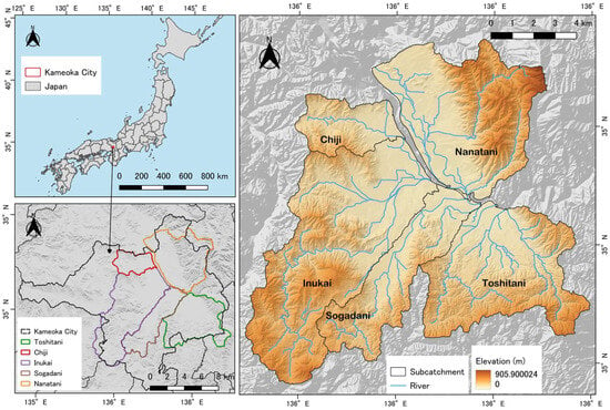
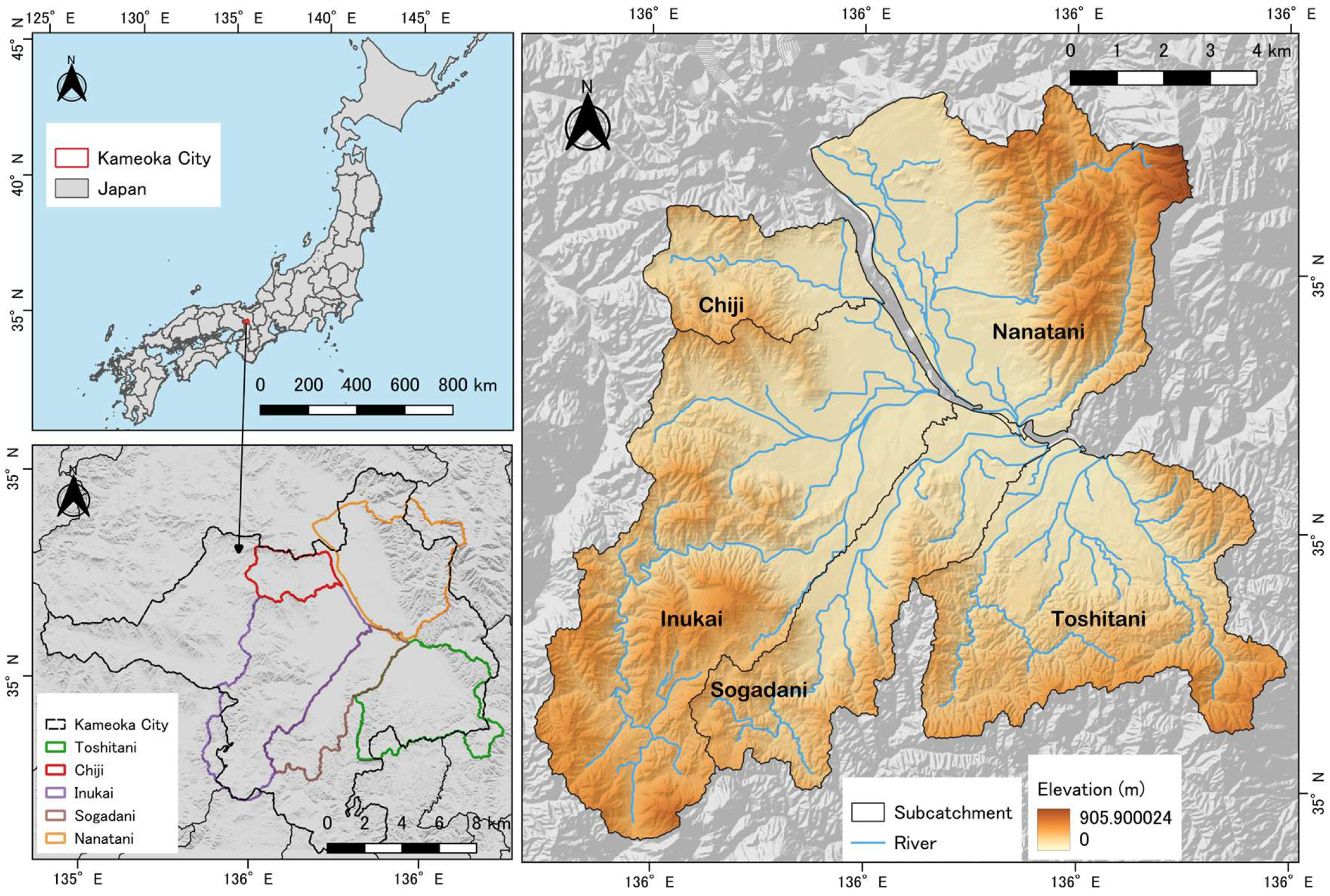
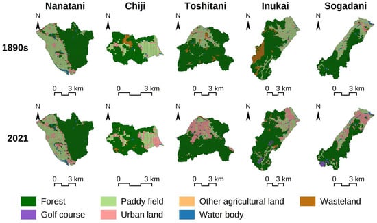
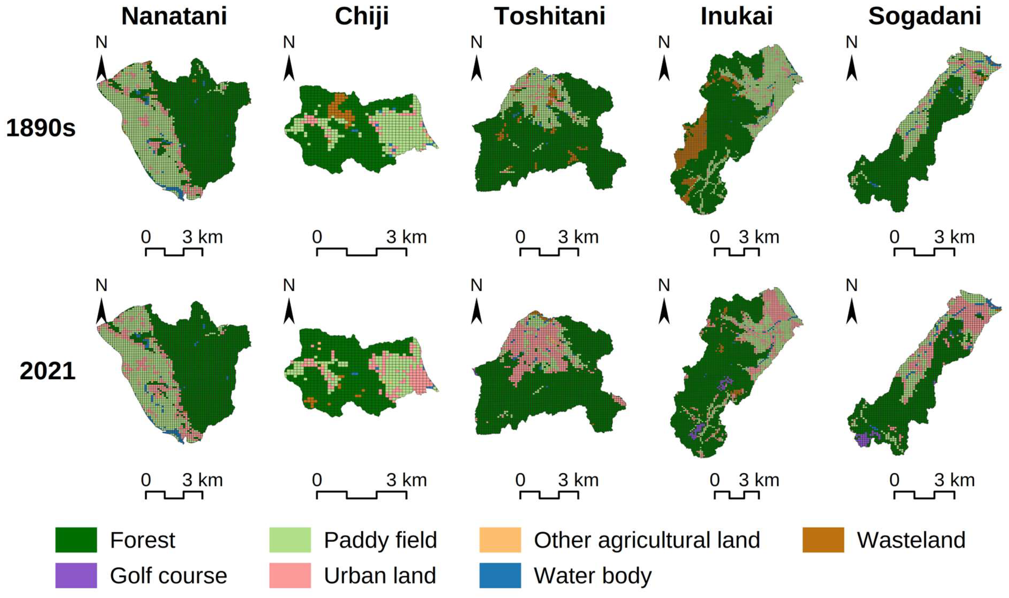
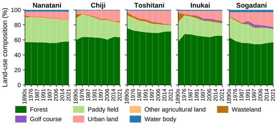
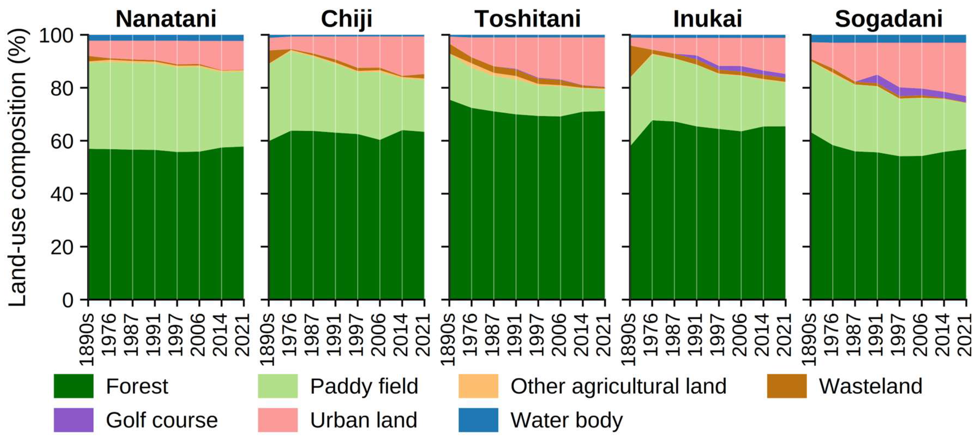
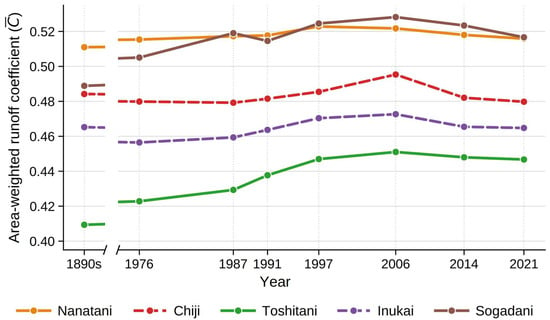
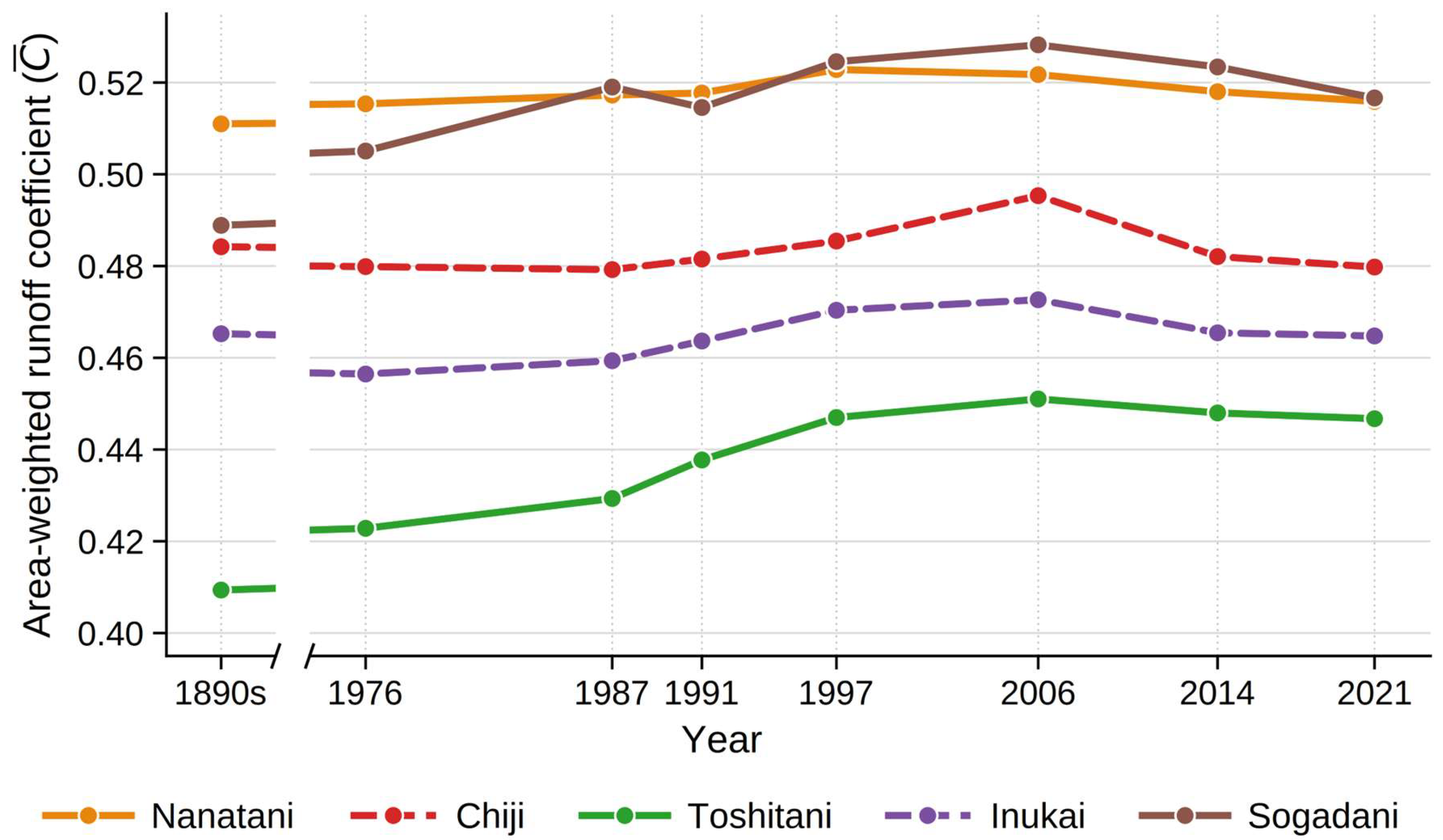
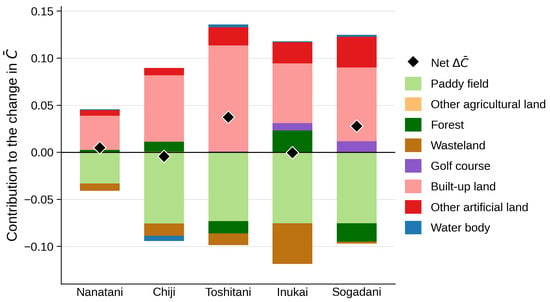
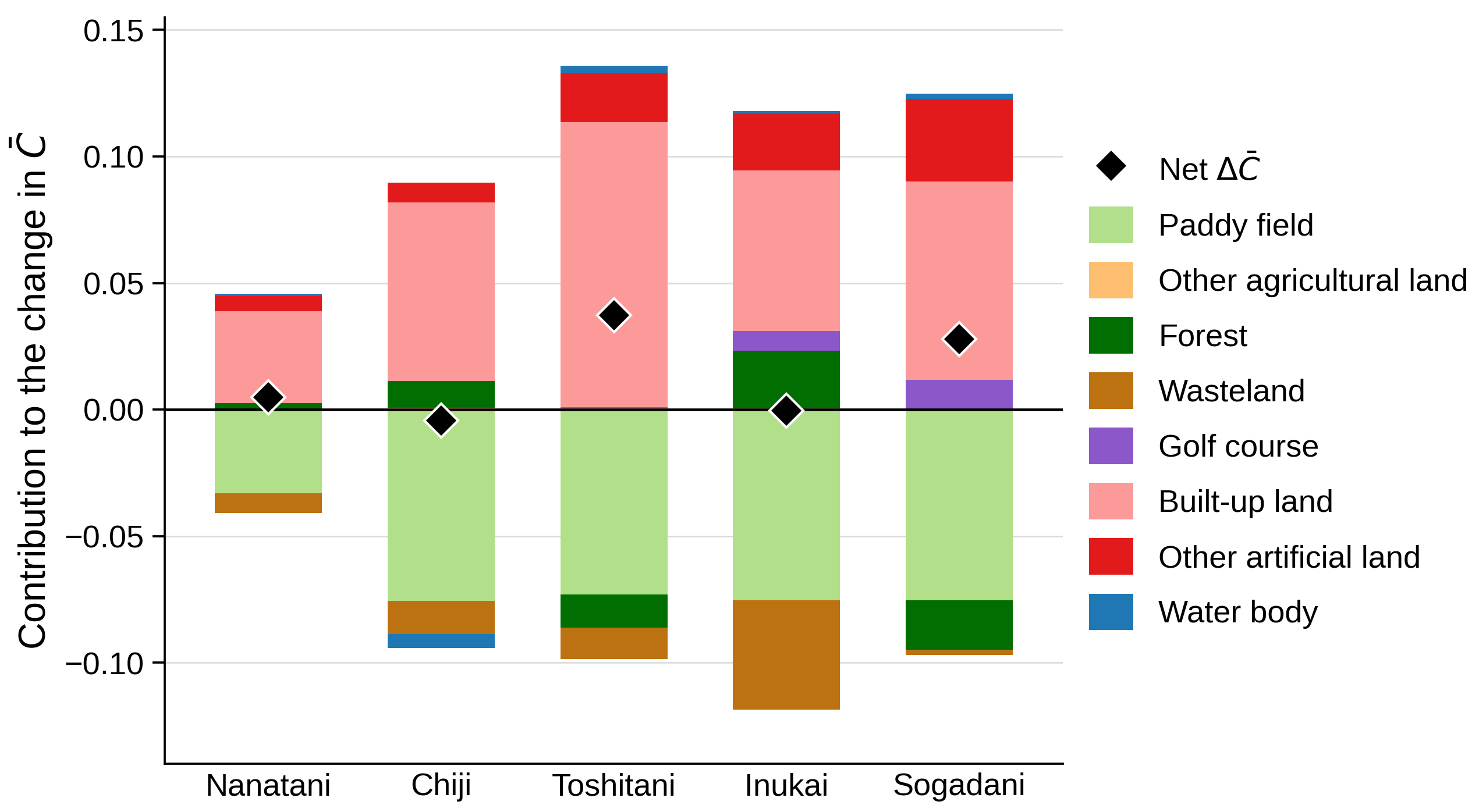
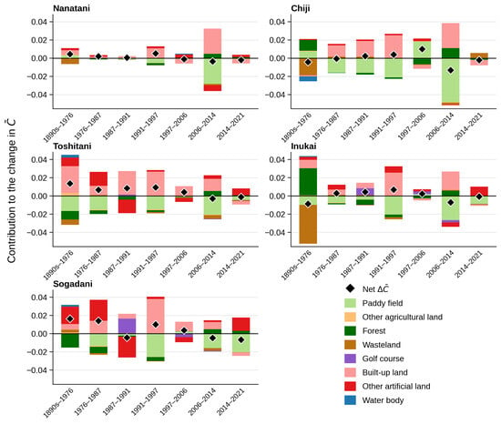
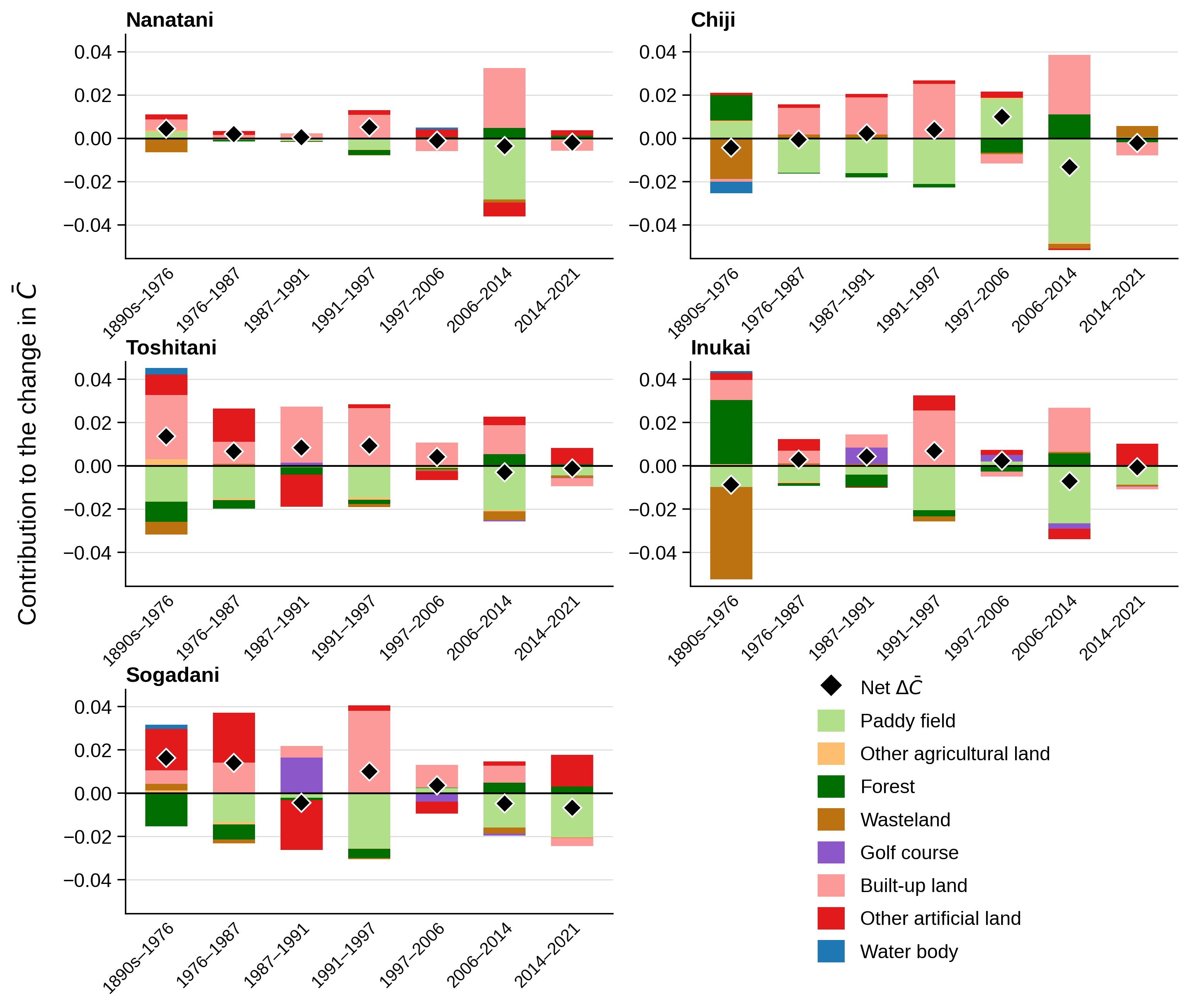

Disclaimer/Publisher’s Note: The statements, opinions and data contained in all publications are solely those of the individual author(s) and contributor(s) and not of MDPI and/or the editor(s). MDPI and/or the editor(s) disclaim responsibility for any injury to people or property resulting from any ideas, methods, instructions or products referred to in the content. |
© 2026 by the authors. Licensee MDPI, Basel, Switzerland. This article is an open access article distributed under the terms and conditions of the Creative Commons Attribution (CC BY) license.