Spatiotemporal Evolution and Associated Factors of Land Use Carbon Emissions on Hainan Island, China

Abstract

Land use reconfiguration can substantially alter regional carbon source–sink patterns, yet integrated evidence remains limited for spatially constrained island systems where development and ecological land are closely juxtaposed. Using Hainan Island (HI) as a case, this study applied an integrated analytical framework linking land use mix, coefficient-based land use carbon emission (LUCE) accounting, spatial redistribution, spatially varying associations, interaction detection, and decoupling analysis across 18 administrative units from 2000 to 2023. Estimated LUCEs increased more than sevenfold during the study period, with emission growth concentrated mainly in coastal development areas, while the interior remained comparatively low in emissions. The spatial distribution of LUCEs gradually expanded inland, and socioeconomic development, built-up land, terrain, and their interactions exhibited heterogeneous associations with LUCEs across the island. The decoupling relationship between land mixed use and LUCEs generally improved after 2005 but remained unstable in several coastal cities. These results indicate that island-wide LUCE evolution is characterized by spatially differentiated relationships between land development and ecological land configuration rather than by a uniform regional process. By integrating land use structure, coefficient-based carbon accounting, spatial redistribution, heterogeneity in factor associations, and decoupling within a common coast–interior framework, this study provides an analytical perspective that can support comparable land use carbon assessments in islands and coastal regions experiencing concentrated development and strong ecological constraints.

1. Introduction

Human-induced greenhouse gas emissions, especially CO₂ from land use and land cover change (LULCC) and fossil fuel burning, have emerged as a major cause of global warming, threatening ecosystem stability and sustainable socioeconomic development [1,2,3]. The IPCC Sixth Assessment Report states that unsustainable resource exploitation and energy use have already increased global mean temperature by about 1.1 °C relative to the pre-industrial level, while extreme weather events such as heatwaves, floods, and droughts are becoming more frequent, further increasing ecosystem vulnerability [4,5]. To address this global challenge, the Paris Agreement calls for limiting the global temperature increase to 1.5 °C and commits signatory nations to the development of long-term pathways for greenhouse gas mitigation [6,7,8]. In this context, China announced its “dual-carbon” goals in 2020, aiming to achieve carbon peaking by 2030 and carbon neutrality by 2060 [9].

Land use change affects regional carbon budgets through both the expansion of emission-intensive land uses and changes in the distribution of ecological land [2,3,10]. Previous studies on Hainan Island (HI) have examined forest biomass, carbon sink dynamics, and carbon storage changes associated with land use transformation [11,12,13]. However, less attention has been given to how the island-wide configuration of development land and ecological land is associated with the spatial differentiation of LUCEs across administrative units.

Under China’s dual-carbon strategy, identifying the spatiotemporal patterns and associated factors of land use carbon emissions (LUCEs) across different geographic units has become important for regional mitigation and spatial governance [14]. Island regions are particularly relevant to carbon management because limited land resources, development concentrated along coastlines, and the close spatial juxtaposition of human activities and forest-dominated ecological areas can intensify the trade-offs between land development, ecological conservation, and carbon regulation [15,16,17]. Globally, these pressures are becoming increasingly pronounced on tropical islands experiencing tourism-driven urbanization, infrastructure expansion, and economic restructuring [18,19]. In China, they are especially relevant to HI, where rapid coastal development coincides with extensive forest conservation in the island’s interior [20]. This close spatial juxtaposition of coastal development and inland ecological areas may generate marked sub-regional differences in development pressure and LUCEs, making a coast–interior perspective particularly relevant for regional land use and carbon analysis [21,22].

Currently, LUCEs are mainly estimated using the carbon emission factor method (CEFM) [23], life cycle assessment [24], and carbon footprint models [25]. Among various approaches, the CEFM is predominantly employed at the macro scale because of its accessibility, standardization, and broad applicability [26]. In parallel, statistical models such as geographically weighted regression (GWR) have been widely adopted to explore the drivers of LUCEs, including demographic, economic, and technological factors [27,28]. In addition, the Tapio decoupling model has become an important tool for evaluating the relationship between LUCEs and economic growth, providing insight into regional mitigation performance and efficiency [29].

Although these approaches have enabled LUCE estimation, spatial pattern identification, driver analysis, and decoupling assessment at national [5], provincial [30], urban agglomeration [31], watershed [32], and coastal region [33], these dimensions have generally been examined separately. Existing studies have also focused predominantly on mainland administrative regions and rapidly urbanizing metropolitan areas. For tropical islands, it therefore remains insufficiently understood how concentrated coastal development and inland ecological conservation are associated with the spatial differentiation of LUCEs, how natural and socioeconomic associations vary across administrative units, and how these spatial differences correspond to decoupling trajectories. To address these gaps, we jointly examine land use structure, coefficient-based LUCEs, spatial redistribution, heterogeneous associations, factor interactions, and decoupling relationships from a coast–interior perspective.

HI provides a suitable case for applying this framework because of its pronounced spatial contrast between rapidly developing coastal areas and a forest-dominated mountainous interior. The island supports diverse ecosystems, including tropical rainforests, mangroves, and coastal wetlands, while population, tourism, infrastructure, and major economic activities are concentrated mainly in coastal cities [34]. In recent years, the construction of the Hainan Free Trade Port (HFTP) has accelerated economic development and increased the demand for urban expansion, infrastructure construction, and land-resource allocation [35]. At the same time, ecological conservation remains a fundamental requirement of regional development, creating a distinct development–conservation context for examining the spatiotemporal evolution of LUCEs.

In view of this, we take HI as the study area and examine the spatiotemporal evolution of LUCEs, its spatially heterogeneous associations with natural and socioeconomic factors, and its decoupling relationship with land mixed use. We test three hypotheses. First, we hypothesize that LUCE exhibits a pronounced coast–interior differentiation, with higher estimated emissions concentrated in development-intensive coastal areas and lower values in the less-developed interior. Second, we hypothesize that the associations between LUCEs and natural and socioeconomic factors vary across administrative units and that interactions among these factors provide greater explanatory power than individual factors alone. Third, we hypothesize that the relationship between changes in land use mix and LUCEs is spatially and temporally heterogeneous, resulting in different decoupling states among administrative units and development periods. Through these analyses, we seek to clarify where and how LUCE changes occur and how their spatial differentiation is associated with the island’s coast–interior development–conservation structure. The combined analytical workflow and coast–interior perspective may also offer a useful reference for LUCE assessments in other tropical islands and coastal regions characterized by constrained land resources, concentrated development, and strong ecological conservation pressures.

2. Materials and Methods

2.1. Study Area

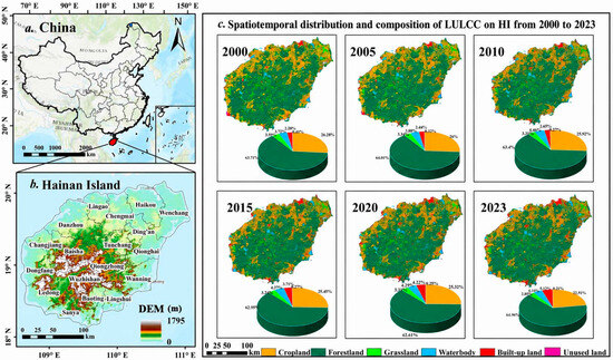
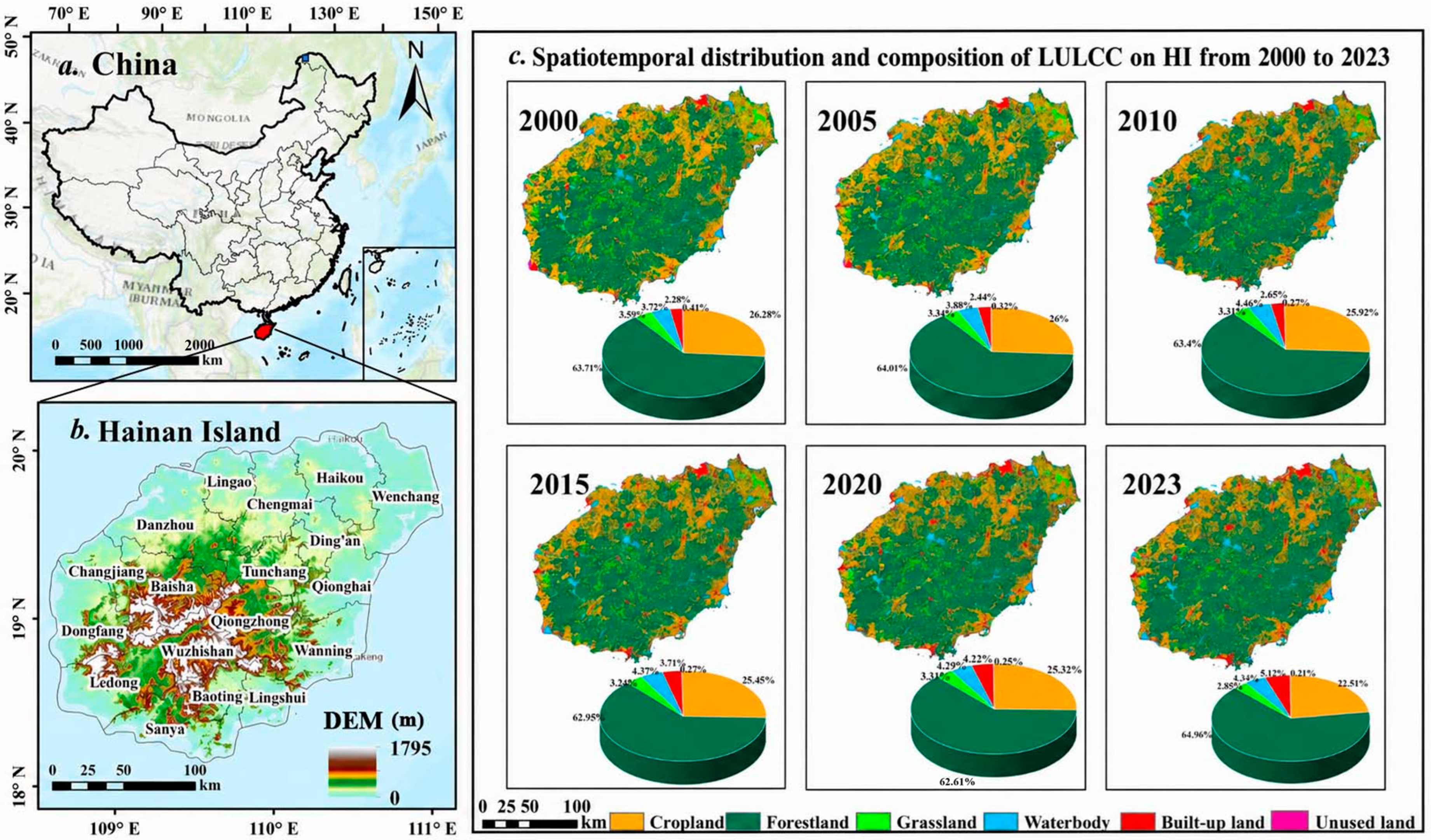
HI is located in southern China (18°10′–20°10′ N, 108°37′–111°03′ E) and covers an area of approximately 33,900 km² (Figure 1). Its terrain is characterized by a high-elevation central region that gradually descends toward the surrounding coastal zones, forming a sequence of mountains, hills, terraces, and coastal plains. HI has a tropical monsoon climate, with mean annual temperatures ranging from 22 °C to 27 °C and annual precipitation of 1600 to 2400 mm. The region is characterized by high temperature, high humidity, abundant sunshine, and sufficient rainfall, giving it relatively high ecological and environmental quality in China [22,36]. Forestland is the dominant land use category on HI, occupying approximately two-thirds of the island and forming an extensive forest-dominated landscape in the central mountainous region. This region contains the principal tropical rainforest ecosystems of HI, including the core areas of Hainan Tropical Rainforest National Park, and plays an important role in biodiversity conservation, watershed regulation, and regional carbon sequestration [37]. In contrast, population, infrastructure, built-up land, and major economic activities are concentrated mainly in the surrounding coastal plains. This spatial configuration produces a pronounced contrast between the ecological functions supported by inland forests and the land development pressure concentrated along the coast. The construction of the HFTP has accelerated urbanization and increased land development pressures on HI. Major development activities are concentrated in coastal cities such as Haikou, Sanya, and Danzhou [21,38].

Figure 1. (a) China. (b) HI. (c) LULCC distribution and composition in 2000, 2005, 2010, 2015, 2020, and 2023.

At the policy level, the Master Plan for the Construction of the HFTP, available online: https://www.gov.cn/zhengce/2020-06/01/content_5516608.htm (accessed on 10 July 2025), released in 2020, established a development framework that combines high-level economic opening with ecological conservation. Meanwhile, the Hainan Territorial Spatial Plan (2021–2035), available online: https://lr.hainan.gov.cn/xxgk_317/0200/0202/202404/t20240424_3652621.html (accessed on 12 July 2025) emphasizes coordinated land–sea development and the protection of ecological conservation red lines, permanent basic farmland, and urban development boundaries. Against this background, Hainan faces the practical challenge of reconciling land development, ecological protection, and carbon mitigation. Its pronounced coast–interior contrast and evolving policy context of HFTP make it a suitable regional case for examining the spatial differentiation of LUCE and its drivers.

2.2. Data

The dataset used for LULCC analysis was obtained from the Data Center for Resources and Environmental Science (available online: https://www.resdc.cn), and comprised six temporal snapshots for 2000, 2005, 2010, 2015, 2020, and 2023 at a spatial resolution of 30 m. Following the original classification system, the data were grouped into six land use and land cover categories: cropland, forestland, grassland, water body, built-up land, and unused land. The temporal interval was five years from 2000 to 2020 and three years between 2020 and 2023. In this study, LULCC refers to the spatiotemporal changes and transitions among different land use and land cover categories during the study period. This classification is consistent with the major land use categories recommended by the IPCC greenhouse gas inventory framework and was adopted based on the original classification system of the Center dataset to facilitate land use carbon emission estimation in the Chinese context. All spatial datasets were uniformly projected using WGS_1984_UTM_Zone_49N with a spatial resolution of 30 m. Energy consumption statistics and socioeconomic data were obtained from the Hainan Statistical Yearbook, available online: https://stats.hainan.gov.cn/tjj/tjsu/ndsj/2025/18gb_list.html (accessed on 4 June 2025). Energy consumption data covered four major energy types: coal, petroleum products, natural gas, and electricity, which were used to estimate energy-related carbon emissions. Socioeconomic indicators, including gross domestic product (GDP), the proportions of secondary and tertiary industries, and the proportion of built-up land area, were selected to characterize regional economic development, industrial structure, and human activity intensity for the analysis of factors associated with LUCE. Digital elevation model (DEM) data were obtained from the Geospatial Data Cloud (available online: https://www.gscloud.cn) and were used to represent topographic conditions in the analysis of factors associated with LUCEs. These statistical data were organized for the six study years and matched to the corresponding administrative units before being incorporated into subsequent analyses. No additional spatial interpolation or resampling was applied to the statistical datasets because they were originally collected at the administrative statistical scale.

2.3. Methods

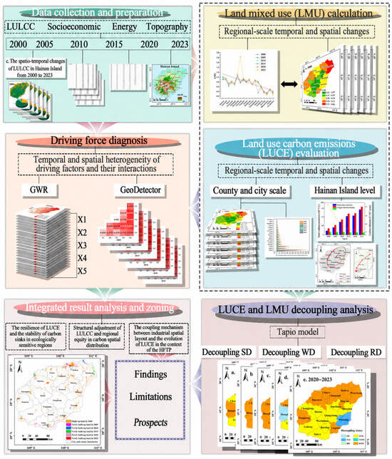
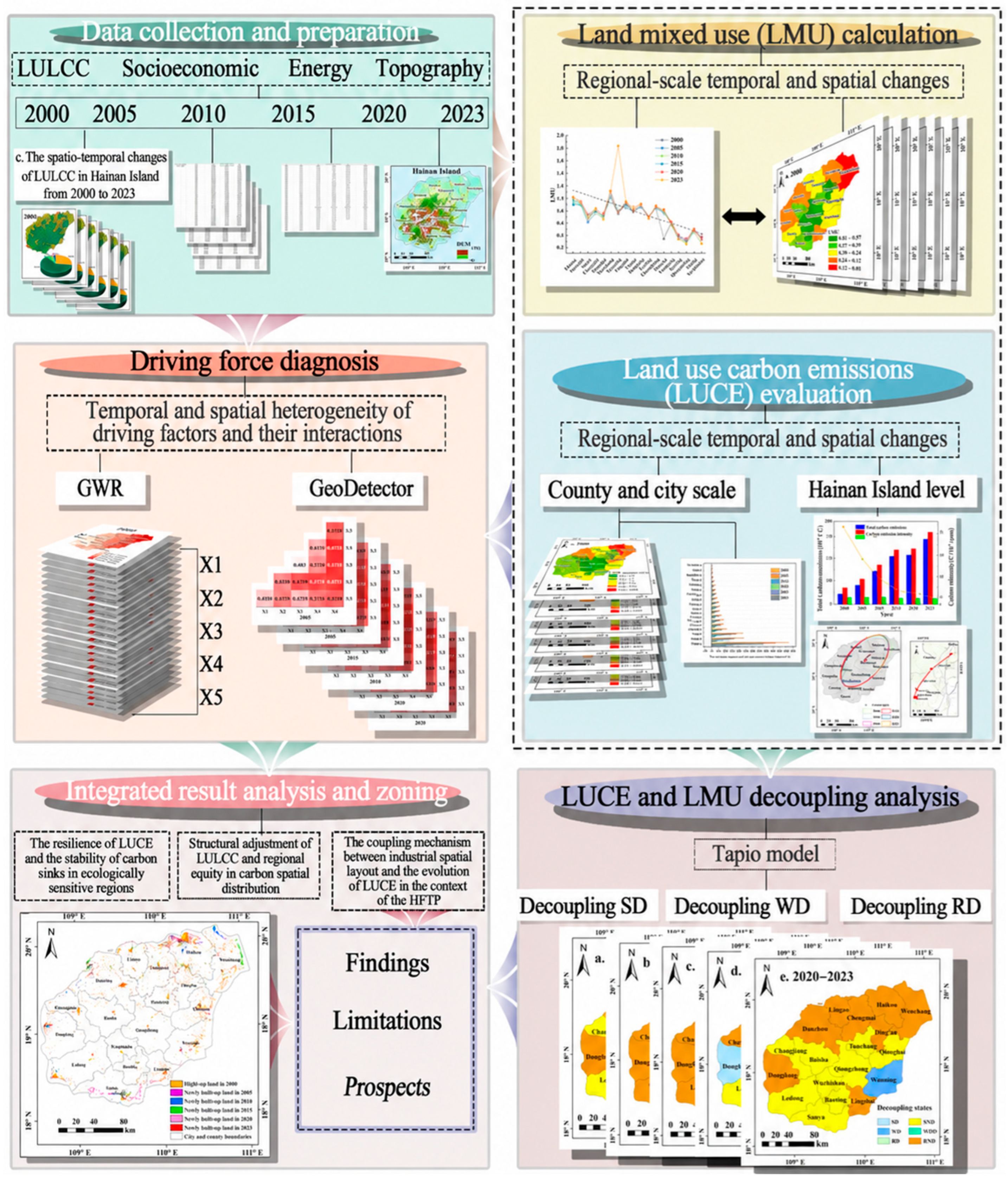
The technical framework underpinning this study is illustrated in Figure 2. The analysis began with the collection and preparation of multitemporal LULCC data, socioeconomic and energy statistics, and topographic data. LMU and LUCEs were subsequently calculated to characterize their temporal evolution and spatial distribution, while the standard deviational ellipse was used to examine changes in the spatial orientation and distribution of LUCEs. GWR and GeoDetector were then applied to examine spatial variation in the associations between LUCE and the selected factors and to assess their joint explanatory power. The Tapio model was further used to evaluate the decoupling relationship between changes in LMU and LUCEs. Within this framework, forestland is explicitly incorporated through the multitemporal LULCC dataset and the direct LUCE accounting component, in which it represents the dominant ecological land category and the principal coefficient-based carbon sink component on HI. Finally, these analytical components were integrated to characterize the relationships among land use structure, estimated LUCEs, spatial factor associations, and LMU–LUCE decoupling patterns.

Figure 2. Research framework.

2.3.1. Land Mixed Use (LMU)

To quantify the compositional complexity and spatial intermixing of LULCC types within a region, this study uses the LMU index. Developed on the basis of information entropy, this indicator effectively characterizes the distributional balance and the extent of intermixing among multiple LULCC types within a given area [39]. A higher LMU value indicates greater land use diversity and a more complex spatial mosaic, whereas a lower value suggests a more homogeneous LULCC. The calculation formula is provided below:

$$LMU=-{\displaystyle \sum _{i=1}^6\left(\frac{d_i}{S}\times \ln \frac{d_i}{S}\right)}$$

(1)

where LMU represents the LMU index; n denotes the number of LULCC categories; d_i corresponds to the area of the i-th LULCC type within the county; and S indicates the area of that county.

2.3.2. LUCE Estimation

Following the general accounting principles of the IPCC Guidelines for National Greenhouse Gas Inventories, LUCE was estimated using activity data and the corresponding emission or removal factors [40]. Based on the sources and accounting pathways of emissions, LUCE was divided into direct and indirect components [5]. Direct LUCE refers to carbon emissions or removals associated with different land use categories and was calculated using the area of each land use category and its corresponding carbon emission or sequestration coefficient [41]. In this study, energy-related carbon emissions were treated as indirect LUCEs attributable to built-up land. These emissions were estimated using the consumption of major energy types and their corresponding emission factors, following the IPCC energy sector accounting approach [40]. The emission and sequestration coefficients assigned to individual land use categories were compiled from published studies conducted in China, taking into account their compatibility with the land use classification and regional environmental context of this study. The calculation formula is provided below:

$$E_p={\displaystyle {\displaystyle \sum _{i=1}^5}{l}_i}={\displaystyle {\displaystyle \sum _{i=1}^5}{A}_i\times {\delta }_i}$$

(2)

where E_p denotes the total LUCEs (t); l_i represents LUCEs from the i-th LULCC type (t); A_i corresponds to the area of the i-th LULCC type (hm²); and δ_i is the corresponding carbon emission coefficient for the i-th LULCC type, expressed in t/(hm²·a). To maintain consistency with regional-scale LUCE studies and because spatially explicit forest inventory data were unavailable for all study years, this study adopted literature-based average coefficients. These coefficients provide comparable regional estimates but cannot fully capture differences in forest age, biomass density, degradation status, management practices, and ecosystem condition. Accordingly, the resulting carbon sink estimates represent generalized regional approximations derived primarily from changes in land use area, rather than direct measurements of actual ecosystem carbon sequestration dynamics (Table 1) [42]. Moreover, the carbon sink offset ratio was calculated as the absolute magnitude of estimated carbon sinks divided by total carbon sources. A higher ratio indicates that a larger proportion of carbon source emissions is offset by the estimated carbon sinks, whereas a lower ratio indicates weaker sink compensation relative to carbon sources [43].

Table 1. Direct LUCE coefficients.

Land Types	Carbon Emission Coefficient	Carbon Effect	Source
Cropland	0.444	Carbon source	[42,44,45]
Forestland	−0.611	Carbon sink
Grassland	−0.021	Carbon sink
Water body	−0.253	Carbon sink
Unused land	−0.005	Carbon sink

Indirect carbon emissions refer to emissions generated by production activities on built-up land [42]. Owing to the considerable uncertainty in the direct carbon emission coefficient of built-up land, previous studies have commonly used fossil energy consumption as a proxy for indirect emissions [46]. Following this approach, this study estimated indirect carbon emissions using the main energy types reported in the Hainan Statistical Yearbook, including coal, electricity, natural gas, and oil. The corresponding coefficients are shown in Table 2. The calculation formula is provided below:

$$E_t={\displaystyle \sum _{i=1}^4{E}_i\times {\rho }_i\times {\theta }_i}$$

(3)

where E_t indicates total energy-related carbon emissions (t); E_i represents the terminal use of the i-th fossil energy (t); ρ_i is the standard coal conversion coefficient for the i-th energy; and θ_i is the carbon emission coefficient for the corresponding energy.

Table 2. LUCE coefficients for different energy types.

Energy Types	Standard Coal Conversion Coefficients	Carbon Emission Coefficients
Coal	0.7143 kgce/kg	0.7559
Oil	1.4286 kgce/kg	0.5857
Electricity	0.1229 kgce/kW·h	0.2132
Natural gas	1.2143 kgce/m3	0.4483

In addition, because consistent fossil energy consumption data at the city and county levels were unavailable for the entire study period, GDP was used as a proxy to spatially allocate indirect carbon emissions among administrative units. GDP-related indicators have also been adopted in previous county-scale carbon-emission studies when finer-scale energy consumption data were unavailable [47,48]. This approach assumes that the spatial distribution of energy-related emissions is broadly proportional to economic output. However, differences in industrial structure, energy intensity, tourism dependence, transportation activity, and production technology may lead to deviations from this assumption, because the carbon-emission performance of different industries and land use functions can vary substantially [49]. The calculation formula is presented below:

$$G_i=E_t\times {\displaystyle \frac{GD{P}_a}{GDP}}$$

(4)

where G_i indicates the energy-related carbon emissions allocated to the i-th city or county (t); GDP_a is the GDP of city or county a in the given year (×10⁴ yuan); GDP is the total GDP of HI in the same year (×10⁴ yuan).

2.3.3. Standard Deviational Ellipse

The standard deviational ellipse was originally introduced as a method for measuring geographic concentration [50]. In this study, it was used to characterize the central location, directional orientation, and spatial extent of LUCE [51,52]. The centroid coordinates represent the center of gravity of LUCE and can be used to trace its migration path over time, thereby revealing changes in LUCE spatial patterns. The calculation is as follows:

$$\overline{Xw}={\displaystyle \frac{{\displaystyle {\sum }_{i=1}^n{w}_i{x}_i}}{{\displaystyle {\sum }_{i=1}^n{w}_i}}}\overline{Yw}={\displaystyle \frac{{\displaystyle {\sum }_{i=1}^n{w}_i{x}_i}}{{\displaystyle {\sum }_{i=1}^n{w}_i}}}$$

(5)

$${\delta }_x=\sqrt{{\displaystyle \frac{{\displaystyle {\sum }_{i=1}^n{(w_i\overline{x_i}\cos \theta -w_i\overline{y_i}\sin \theta )}^2}}{{\displaystyle {\sum }_{i=1}^n{w}_i^2}}}}$$

(6)

$${\delta }_y=\sqrt{{\displaystyle \frac{{\displaystyle {\sum }_{i=1}^n{(w_i\overline{x_i}\sin \theta -w_i\overline{y_i}\cos \theta )}^2}}{{\displaystyle {\sum }_{i=1}^n{w}_i^2}}}}$$

(7)

$$\tan \theta ={\displaystyle \frac{({\displaystyle {\sum }_{i=1}^{n}w{i}^2}\overline{x{i}^2}-{\displaystyle {\sum }_{i=1}^{n}wi\overline{y{i}^2}})+\sqrt{{\displaystyle {\sum }_{i=1}^{n}w{i}^2}\overline{x{i}^2}-{\displaystyle {\sum }_{i=1}^n{\mathrm{w}}_i\overline{y{i}^{2}2+4{\displaystyle {\sum }_{i=1}^{n}w{i}^2}\overline{x{i}^{2}y{i}^2}}}}}{2{\displaystyle {\sum }_{i=1}^{n}w{i}^2}\overline{x{i}^{2}y{i}^2}}}$$

(8)

where $\overline{x{i}^2}$ and $\overline{y{i}^2}$ represent the squared distances from the spatial position coordinates (x_i, y_i) to the center of gravity; w_i denotes the weight, which in this study refers to LUCEs; θ is the azimuth angle of the standard deviational ellipse; and ${\delta }_x$ and ${\delta }_y$ are the standard deviations along the x and y axes, respectively.

2.3.4. GWR Model

GWR was originally developed to examine spatial nonstationarity in relationships between variables [53]. Unlike ordinary least squares regression, GWR allows regression coefficients to vary across space and thereby captures local differences in the relationships between the dependent and explanatory variables [54,55]. Before applying GWR, OLS models were fitted separately for each study year using the same dependent and explanatory variables. Variance inflation factors (VIFs) were calculated to assess multicollinearity, the Breusch–Pagan test was used to examine heteroscedasticity, and Global Moran’s I was calculated for the OLS residuals to assess residual spatial autocorrelation [56].

Based on previous LUCE studies and data availability [57,58], DEM (X1), GDP (X2), the proportion of secondary industry (X3), the proportion of tertiary industry (X4), and the proportion of built-up land (X5) were selected as explanatory variables, while LUCE was specified as the dependent variable. These variables represent topographic conditions, economic development, industrial structure, and land development intensity, respectively. Because each annual model was based on 18 city- and county-level spatial units, the GWR analysis was used primarily to explore spatially varying associations. Given the small number of spatial units relative to the number of explanatory variables, the local coefficient estimates may be sensitive to model specification and should therefore be interpreted as exploratory spatial patterns rather than as stable parameter estimates for statistical inference. The local coefficients were not interpreted as causal effects or as definitive statistical evidence of spatial nonstationarity. The calculation formula is provided below:

$$Y_i={\beta }_0\left(u_i,v_i\right)+{\displaystyle \sum _{k=1}^p{\beta }_k\left(u_i,v_i\right)X_{ik}+{\epsilon }_i}\begin{array}{c}(i=1,2,3,\cdots ,n)\end{array}$$

(9)

where $\left(u_i,v_i,t_i\right)$ denotes the spatial coordinates of the i-th research unit; X_ik represents the value of the k-th independent variable at the i-th research unit; ${\beta }_0\left(u_i,v_i,t_i\right)$ is the intercept term; ${\beta }_k\left(u_i,v_i,t_i\right)$ represents the regression coefficient of the k-th independent variable for the i-th unit; ε_i is the residual term.

2.3.5. GeoDetector

GeoDetector is a statistical method for assessing spatially stratified heterogeneity and the explanatory power of potential associated factors. The q-value quantifies the extent to which the spatial stratification of an explanatory variable corresponds to that of the dependent variable [56]. Interaction detection was further used to compare the explanatory power of individual factors with that of paired factors [59]. Accordingly, GeoDetector was applied to quantify the explanatory power of the selected factors for the spatial variation in LUCEs and to examine changes in explanatory power when factors were considered jointly. The calculation formula is provided below:

$$q=1-{\displaystyle \frac{1}{N{\sigma }^2}}{\displaystyle \sum _{h=1}^L{N}_h}{\sigma }_h^2$$

(10)

where q represents the explanatory power of an individual factor or factor combination; L is the number of strata of the explanatory factor; N and N_h denote the sample sizes of the overall study area and sub-region h, respectively; ${\sigma }_h^2$ and ${\sigma }^2$ are the variances of the dependent variable Y within the sub-region and the entire study area. The q-value ranges from 0 to 1, with higher values indicating stronger explanatory power for the dependent variable.

2.3.6. Decoupling Models

Decoupling describes a weakening correspondence between changes in two variables over time [60]. Although the Tapio framework is most commonly applied to economic output and environmental pressure, its elasticity formulation has also been extended to land use and resource use relationships [39,61,62]. In this study, LMU is not used as a proxy for economic growth. Rather, it serves as the reference variable describing changes in land use composition and functional diversity, allowing the elasticity index to characterize whether changes in LUCEs occur proportionally faster or slower than changes in land use mixture. Accordingly, the resulting decoupling states describe the relationship between the relative rates of change in LUCEs and LMU rather than conventional economic growth–emission decoupling [39]. The decoupling index (D) is calculated using the change rates of LMU (ΔLMU) and LUCEs (ΔEP), as follows:

$$D={\displaystyle \frac{\Delta EP}{\Delta LMU}}={\displaystyle \frac{\left(E{P}_s-E{P}_r\right)/E{P}_r}{\left(LM{U}_s-LM{U}_r\right)/LM{U}_r}}$$

(11)

where D is the decoupling index from years r to s; EP_s and EP_r represent the LUCE index in years s and r, respectively; LMU_s and LMU_r denote the land mixed use index in years s and r, respectively. Under the Tapio model, decoupling relationships are divided into three overarching categories and eight specific decoupling states (Table 3).

Table 3. Classification criteria for the decoupling states between LMU and LUCEs.

Category	Decoupling State	ΔEP	ΔLMU	D	Description
Decoupling	Strong decoupling (SD)	<0	>0	<0	LMU increases while LUCE decreases.
	Weak decoupling (WD)	>0	>0	0 < D < 0.8	LMU grows faster than LUCE.
	Recessive decoupling (RD)	<0	<0	>1.2	LMU declines more slowly than LUCE.
Negative Decoupling	Strong negative decoupling (SND)	>0	<0	<0	LMU decreases whereas LUCE increases.
	Weak negative decoupling (WND)	<0	<0	0 < D < 0.8	LMU declines faster than LUCE.
	Expansive negative decoupling (END)	>0	>0	>1.2	LMU grows more slowly than LUCE.
Coupling	Expansive coupling (EC)	>0	>0	0.8 ≤ D ≤ 1.2	LMU and LUCE grow at comparable rates.
	Recessive coupling (RC)	<0	<0	0.8 ≤ D ≤ 1.2	LMU and LUCE decline at approximately the same rate.

3. Results

3.1. Spatiotemporal Characteristics of LULCC and LMU

Forestland remained the dominant land use category on HI throughout the study period. Its area increased from 21,827.63 km² in 2000 to 22,250.45 km² in 2023, representing a net increase of 422.81 km², or 1.94%. Built-up land increased by 124.72% during the same period, with expansion mainly concentrated in coastal development areas such as Haikou, Sanya, and Danzhou (Figure 1c). These changes indicate that forestland remained broadly stable with a slight net increase, whereas built-up land expanded much more rapidly. Against this background of LULCC, LMU on HI showed an overall increasing trend.

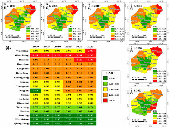
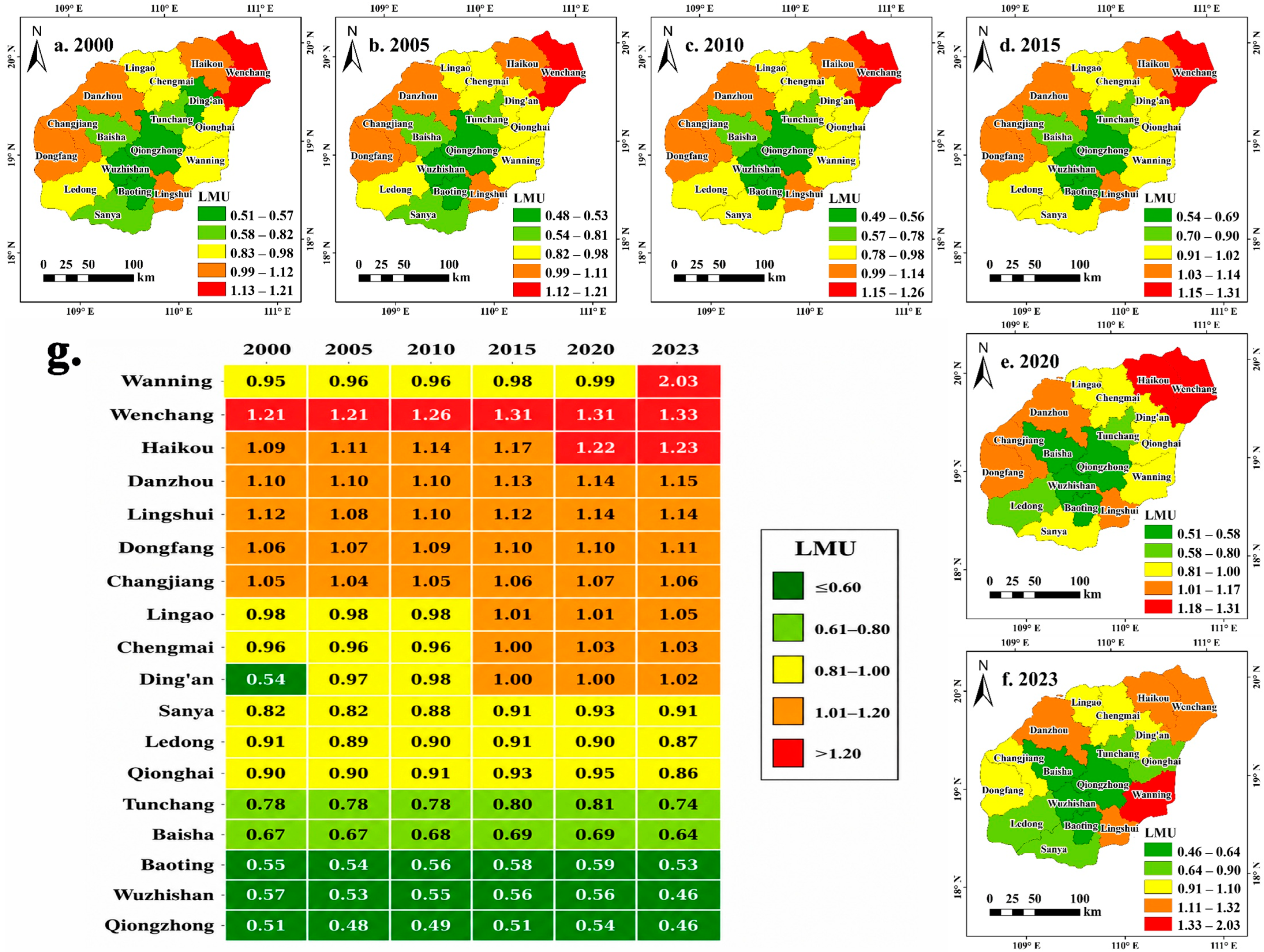
Wenchang consistently had the highest LMU, with an annual average above 1.27, while Qiongzhong, Baoting, and Wuzhishan had the lowest values, generally ranging from 0.50 to 0.56 (Figure 3g). Temporally, LMU remained relatively stable from 2000 to 2010, but increased in most counties after 2010. Haikou, Wenchang, and Chengmai recorded increases of 7.88%, 6.99%, and 5.42%, respectively, during 2010 to 2023. Wanning recorded the largest increase, with its LMU reaching 2.03 in 2023. This pattern indicates an increase in land use heterogeneity in Wanning during the later study period.

Figure 3. (a–f) Spatial characteristics of LMU. (g) Temporal characteristics of LMU.

Spatially, LMU values were generally higher in the northern and coastal counties and lower in the southern and interior counties (Figure 3a–f). Haikou, Wenchang, and Wanning had relatively high LMU values, whereas Wuzhishan, Baisha, and Baoting consistently had lower values. In contrast, low-value areas were consistently distributed in the central and southwestern mountainous counties, including Wuzhishan, Baisha, and Baoting, where forest-dominated landscapes and stronger ecological protection maintained relatively stable land use structures.

3.2. Spatiotemporal Characteristics of LUCE

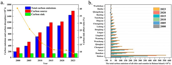
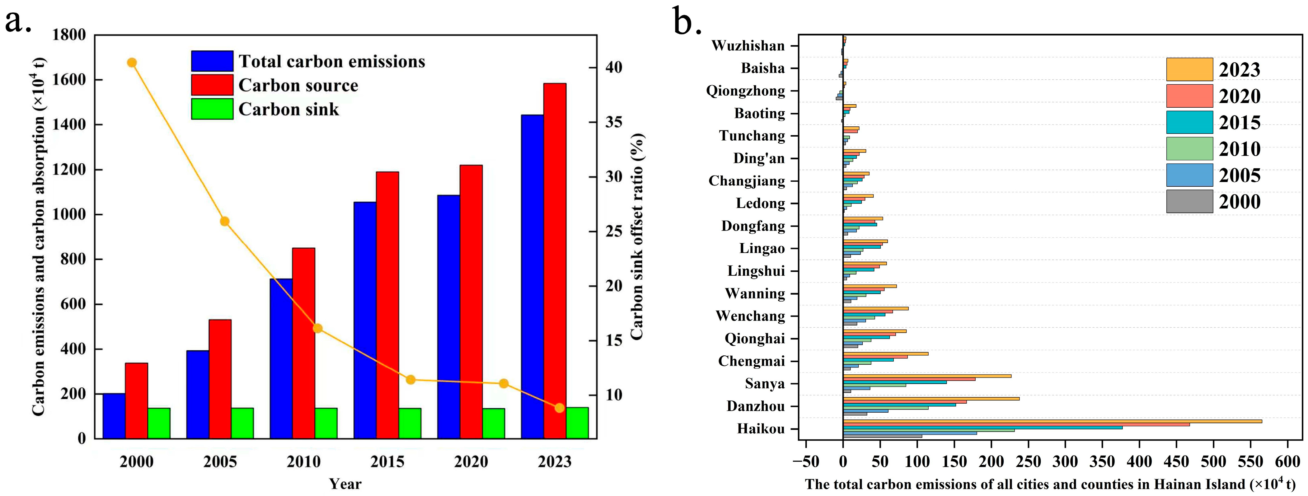
Based on the observed changes in land use areas, energy consumption data, and the corresponding emission or sequestration coefficients, the estimated total LUCEs on HI increased from approximately 201.41 × 10⁴ t in 2000 to 1443.54 × 10⁴ t in 2023 (Figure 4a). During the same period, carbon sources rose from approximately 338.25 × 10⁴ t to 1583.44 × 10⁴ t. LUCE growth showed a phased pattern, with an average annual increase of 51.11 × 10⁴ t from 2000 to 2010 and 56.23 × 10⁴ t from 2010 to 2023. Meanwhile, the carbon sink offset ratio declined from 40.45% to 8.84%, indicating that the estimated carbon sinks offset a progressively smaller proportion of the growing carbon source emissions. This trend was mainly associated with the continued expansion of built-up land and increasing energy consumption, whereas the limited variation in the estimated carbon sinks mainly reflected the relative stability of major ecological land types, particularly forestland.

Figure 4. (a) Overall characteristics of LUCEs on HI. (b) Evolution of estimated LUCE across cities and counties on HI, with administrative units ordered in ascending order according to their 2023 values.

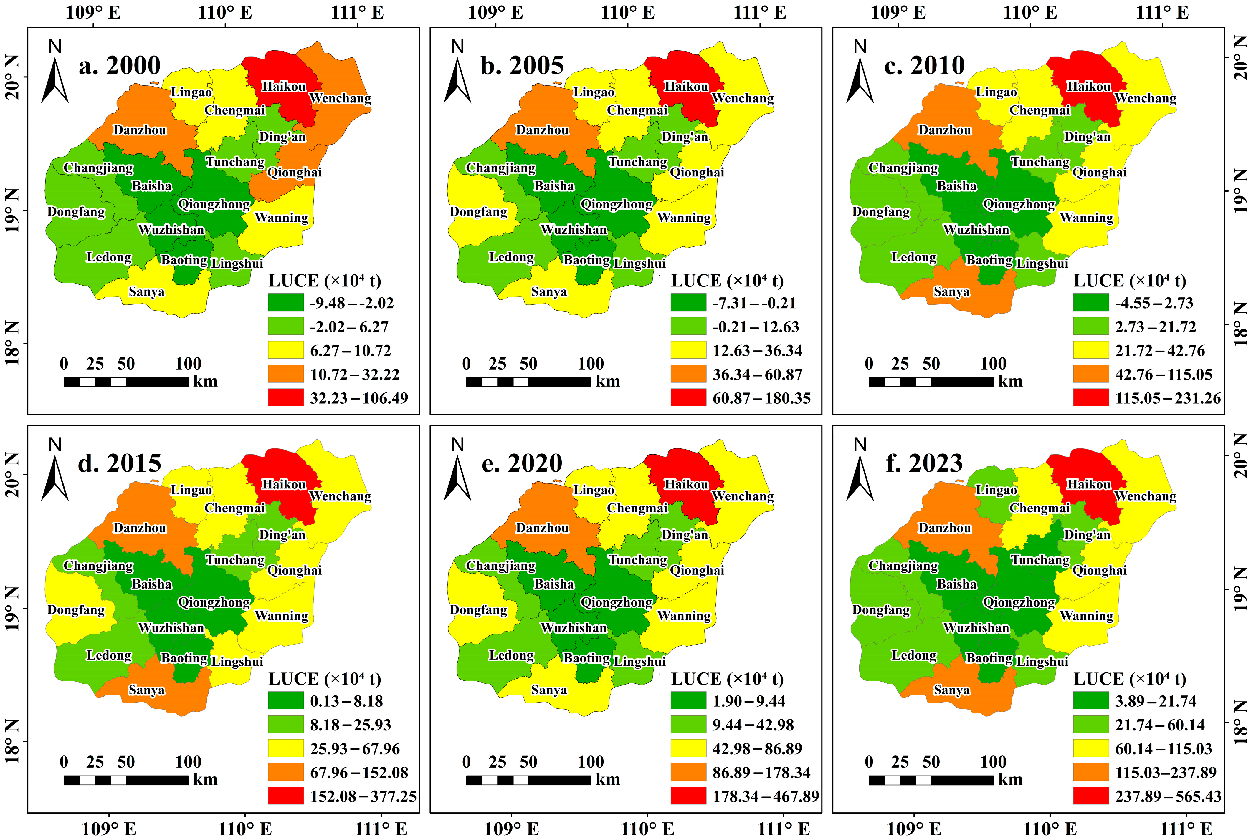
At the county level, LUCEs generally followed the island-wide increasing trend but varied among administrative units (Figure 4b). Haikou consistently recorded the highest LUCEs, rising from approximately 106.49 × 10⁴ t in 2000 to 565.43 × 10⁴ t in 2023. Sanya and Danzhou also increased markedly, by 216.47 × 10⁴ t and 205.67 × 10⁴ t, respectively. Eastern coastal cities such as Qionghai, Wenchang, Wanning, and Lingshui remained at medium levels but showed continuous growth, while Chengmai, Dongfang, and Changjiang in western HI all exceeded 60 × 10⁴ t by 2023. In contrast, Qiongzhong, Baisha, and Wuzhishan consistently maintained low estimated LUCEs, with all three counties remaining below 7 × 10⁴ t in 2023. These low values coincided with forest-dominated land use structures and relatively limited development intensity.

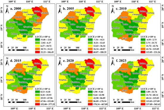
LUCE values were generally higher in the northern and coastal counties and lower in the southern and interior counties (Figure 5). Haikou remained the county with the highest LUCEs and recorded the maximum value in 2023. LUCEs in Wenchang, Danzhou, and Sanya also increased over the study period, and these counties emerged as additional high-LUCE areas. Qionghai, Wanning, and Chengmai remained at intermediate levels, whereas Wuzhishan, Qiongzhong, and Baisha consistently maintained relatively low LUCEs.

Figure 5. Spatial distribution of LUCE across HI in different years: (a) 2000; (b) 2005; (c) 2010; (d) 2015; (e) 2020; and (f) 2023. LUCE values are expressed in units of ×10⁴ t.

3.3. Characteristics of LUCE Centroid Migration

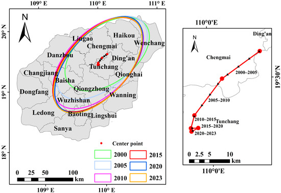
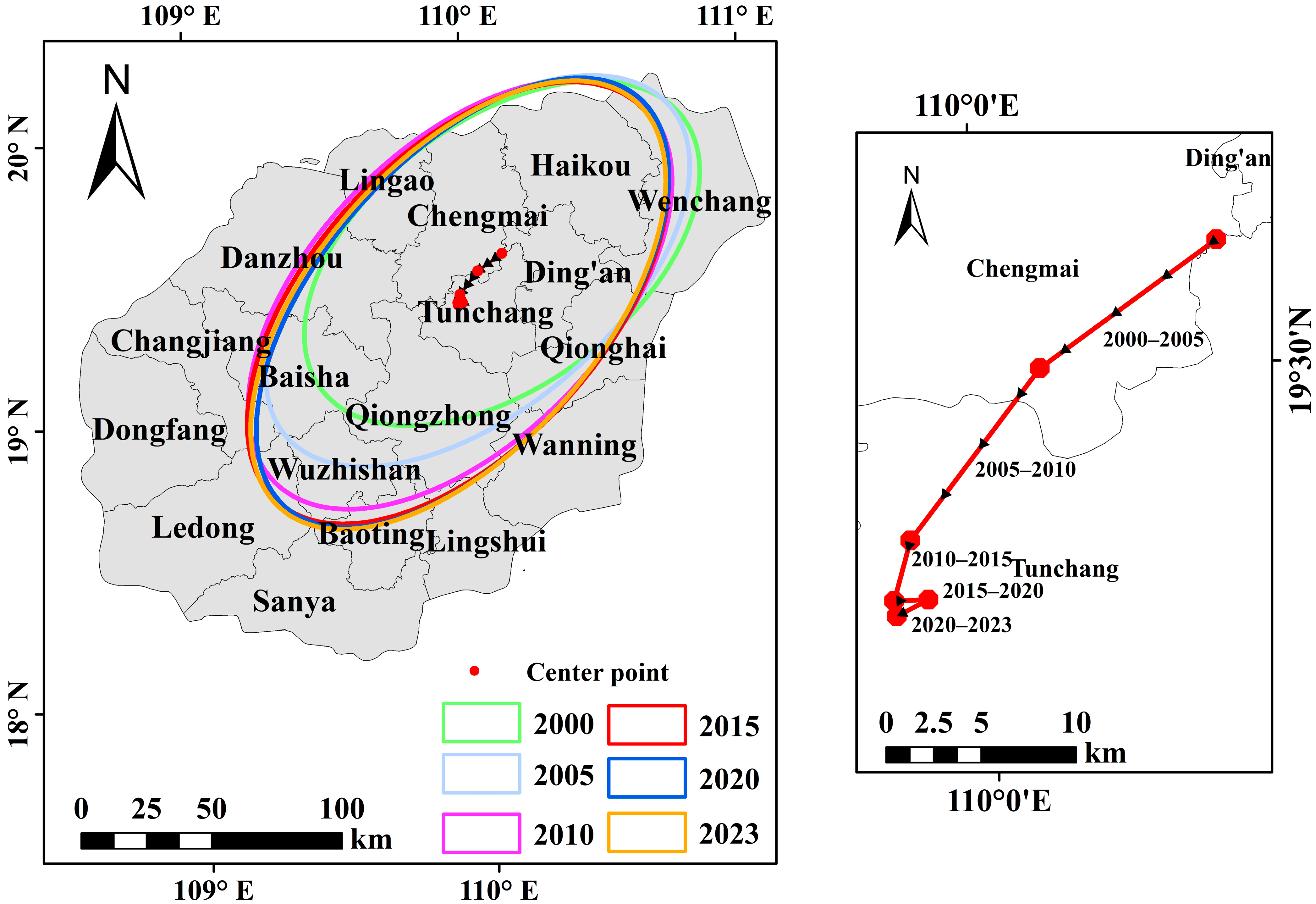
The standard deviational ellipse analysis showed that the ellipse area was relatively small in 2000 and 2005 (Figure 6), indicating a comparatively concentrated spatial distribution of LUCE in northern HI, particularly around Haikou, Wenchang, and Ding’an. After 2010, the ellipse expanded markedly, indicating an increase in the spatial dispersion of LUCE. From 2010 to 2023, the major axis extended southward and the centroid gradually shifted toward the central part of the island, reflecting a directional redistribution of LUCE from the northeastern coastal area toward the interior. The concurrent expansion of the ellipse and displacement of its centroid indicate that LUCE evolution involved not only an increase in total emissions but also a progressive reorganization of their spatial distribution, from a relatively concentrated northern pattern toward a broader coast–interior configuration.

Figure 6. Standard deviational ellipses of LUCEs on HI.

3.4. Spatial Relationships Between LUCE and the Selected Factors

3.4.1. Spatial Variation in the Relationships Between LUCE and the Selected Factors

All annual OLS models were statistically significant (p < 0.001), with adjusted R² values ranging from 0.720 to 0.830, indicating that the selected factors were collectively associated with a substantial proportion of the spatial variation in LUCEs. The maximum VIF values ranged from 5.83 to 7.95, indicating moderate and non-negligible multicollinearity among some explanatory variables, with relatively high values occurring in 2005 and 2020. The Breusch–Pagan test was significant in 2005 (p = 0.040) and 2015 (p = 0.033), suggesting heteroscedasticity in these two annual models. However, Global Moran’s I tests of the OLS residuals were not statistically significant in any study year (permutation p = 0.405–0.843), indicating that residual spatial autocorrelation was not evident under the adopted queen-contiguity spatial-weight specification.

These diagnostics indicate that the selected explanatory factors were collectively related to the spatial variation in LUCEs, but they did not provide uniform statistical evidence of spatial nonstationarity across all study years. GWR was therefore retained as an exploratory analysis to examine how the estimated relationships varied among administrative units. The adjusted R² values of the fitted GWR models exceeded 0.8, while their AICc values remained below 200. These statistics are reported only as descriptive measures of in-sample model fit and were not interpreted independently as evidence that GWR was superior to the corresponding global models or that spatial nonstationarity was definitively established. Given the limited number of spatial units, moderate multicollinearity, and sensitivity to influential observations, the local coefficients were interpreted as spatially varying associations rather than causal effects.

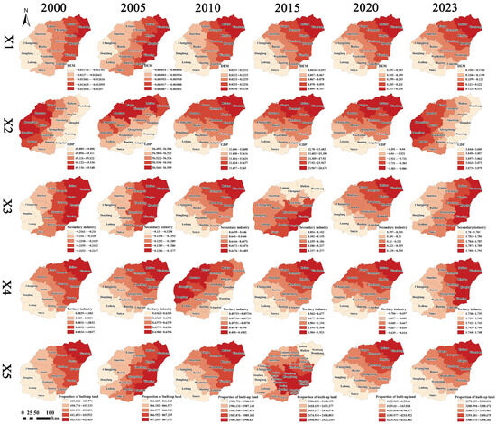
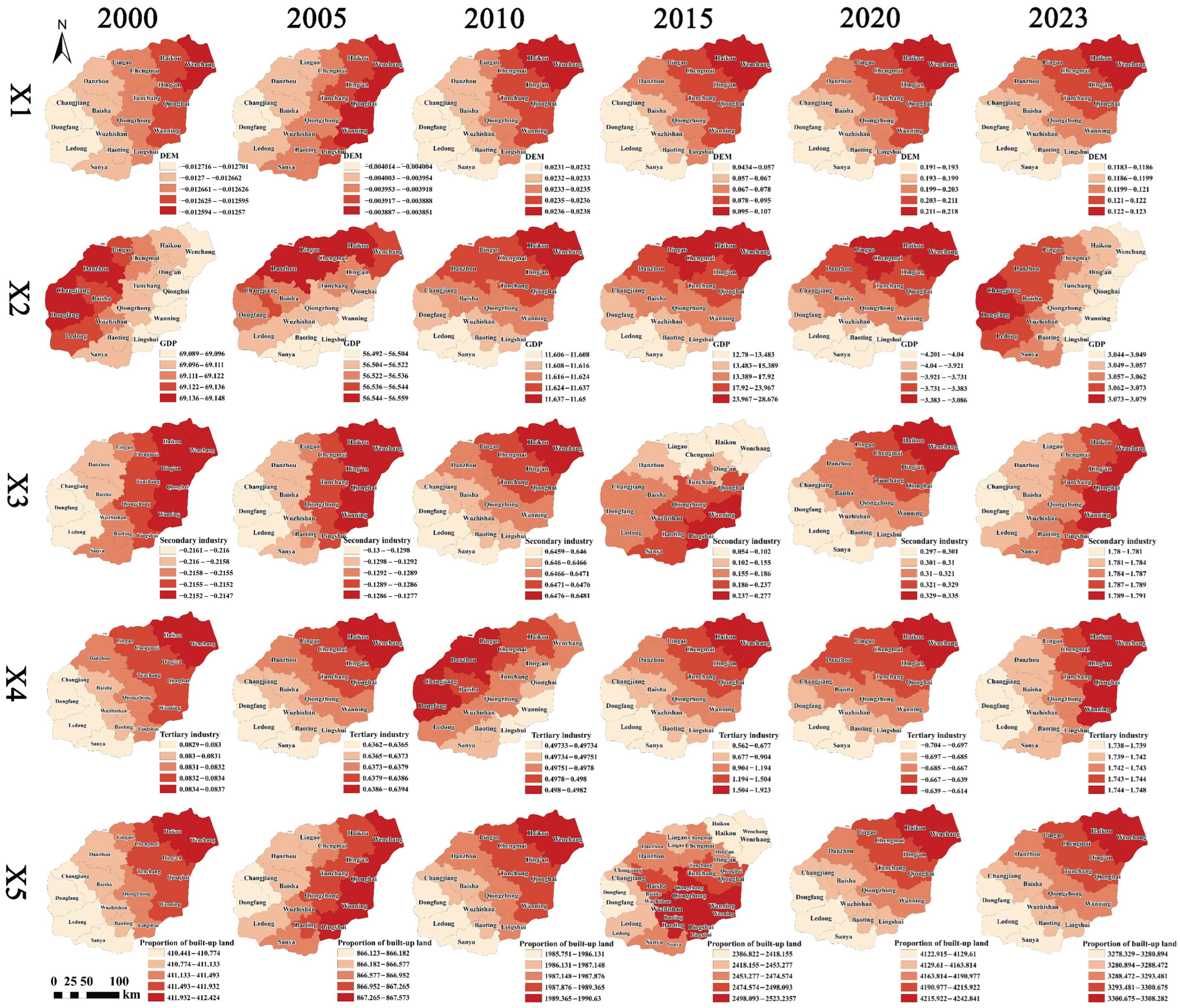
The estimated GWR coefficients for the five explanatory variables varied across administrative units (Figure 7). DEM (X1) was generally negatively associated with LUCEs, with more negative coefficients in the central and southern mountainous counties, including Qiongzhong, Baisha, and Wuzhishan, and weaker associations in the coastal plains. GDP (X2) showed larger positive coefficients in economically active areas such as Haikou, Sanya, and Danzhou, indicating stronger positive associations with LUCEs in these areas. This association should nevertheless be interpreted cautiously because GDP was also used to spatially allocate the indirect emission component of LUCE and is therefore not fully independent of the dependent variable. The proportion of the secondary industry (X3) had relatively high coefficients in northwestern and central counties, indicating a stronger positive association with LUCEs in these areas. The proportion of the tertiary industry (X4) showed relatively high coefficients in service-oriented cities such as Haikou and Sanya. The coefficients for built-up land proportion (X5) became increasingly positive over time and were observed across a broader set of central and southwestern counties.

Figure 7. Spatial distribution of local GWR coefficients for the selected factors associated with LUCE in 2000, 2005, 2010, 2015, 2020, and 2023. Rows X1–X5 represent DEM (X1), GDP (X2), the proportion of secondary industry (X3), the proportion of tertiary industry (X4), and the proportion of built-up land (X5), respectively. Columns represent the six study years. Colors represent the classified values of the local regression coefficients, as indicated by the legend in each panel. Positive coefficients indicate positive associations with LUCE, whereas negative coefficients indicate negative associations.

3.4.2. Interaction Detection of Explanatory Factors

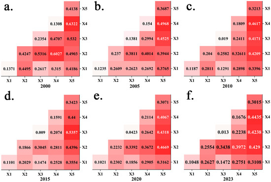
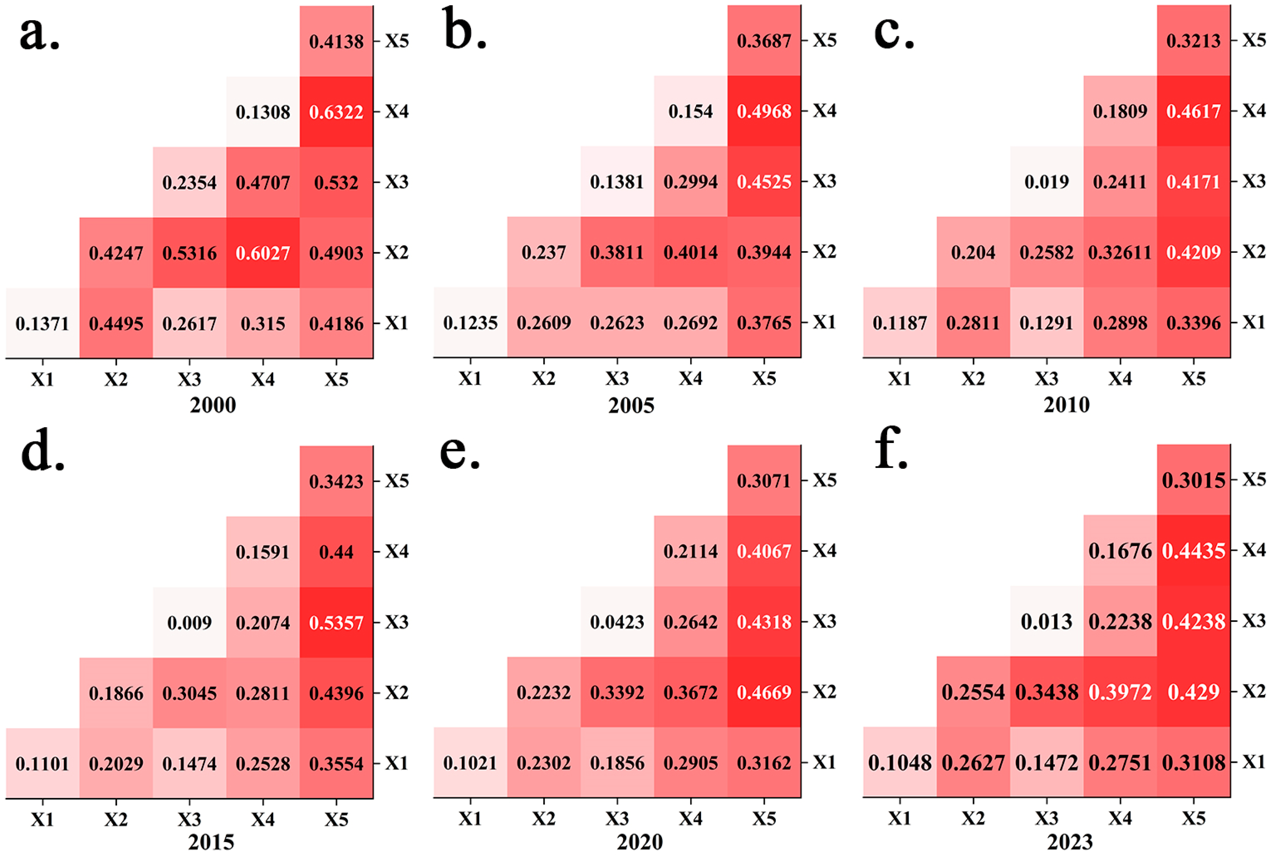
In most years, the q-values of two-factor interactions were higher than those of the corresponding individual factors, indicating greater explanatory power for the spatial differentiation of LUCEs when the factors were considered jointly (Figure 8). Among all factor pairs, the interaction between GDP (X2) and the proportion of the tertiary industry (X4) showed the highest q-values, reaching 0.6027 in 2000 and 0.4435 in 2023, both exceeding the explanatory power of either factor alone. The interaction between GDP (X2) and the proportion of secondary industry (X3) also showed relatively high explanatory power and reached 0.5357 in 2015. In addition, the interaction between the proportion of the tertiary industry (X4) and built-up land proportion (X5) maintained relatively high q-values, ranging from 0.3015 to 0.4138 across the six study years, indicating a persistent joint explanatory relationship with the spatial variation in LUCEs. By contrast, interactions involving DEM (X1) generally had lower q-values, although the interaction between DEM (X1) and GDP (X2) reached 0.4247 in 2000.

Figure 8. Interaction detection results for factors associated with the spatial differentiation of LUCE on HI in different years: (a) 2000; (b) 2005; (c) 2010; (d) 2015; (e) 2020; and (f) 2023. Each cell in the lower triangular matrix shows the q-value of the interaction between two explanatory factors, with darker shading indicating stronger explanatory power. X1–X5 denote DEM, GDP, the proportion of secondary industry, the proportion of tertiary industry, and the proportion of built-up land, respectively.

3.5. LUCE Decoupling Analysis

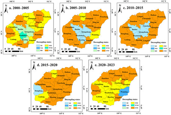
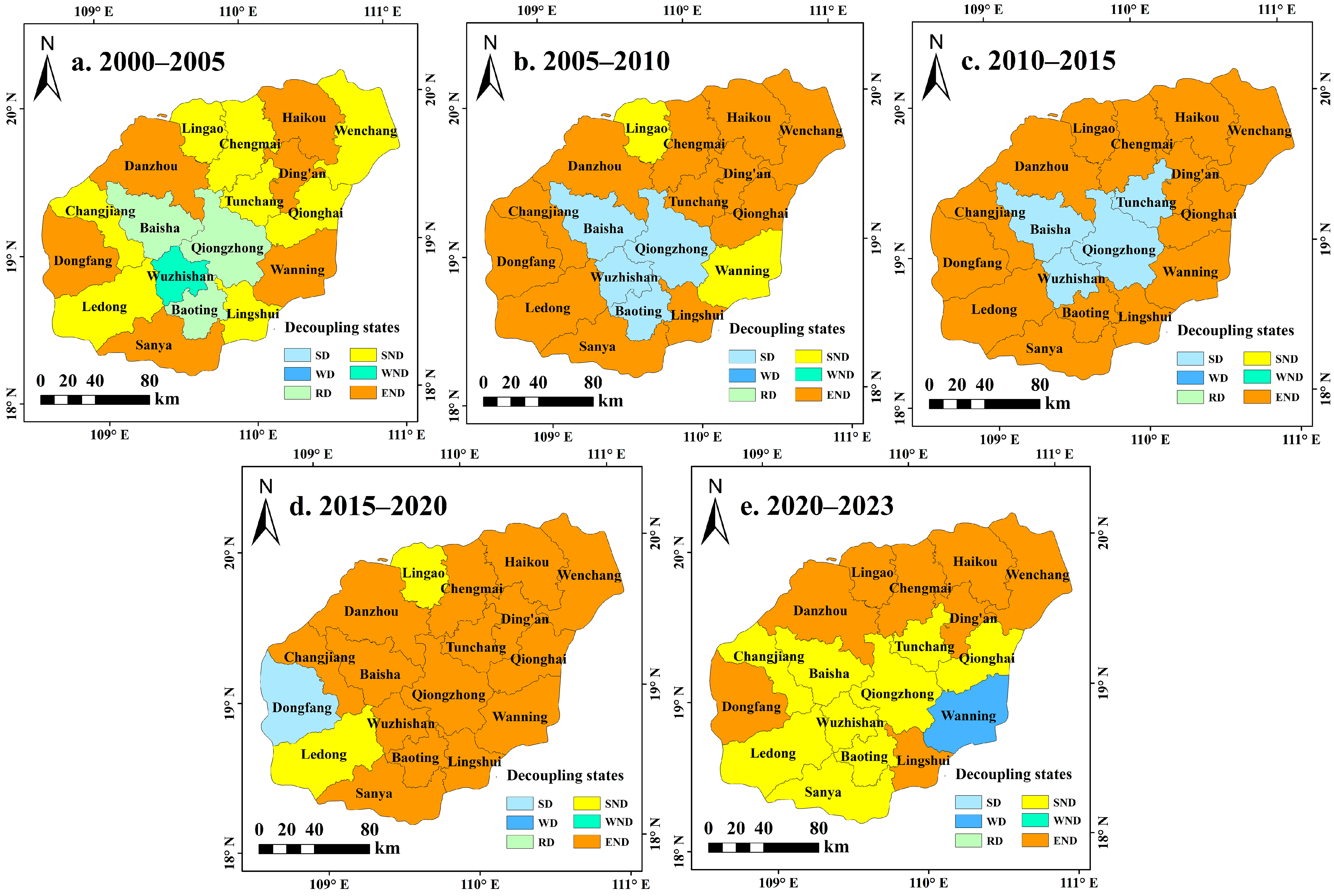
Decoupling states differed between the central ecological counties and several coastal development-oriented counties (Figure 9). From 2000 to 2005, most counties were dominated by END and SND, indicating that LUCEs increased faster than LMU. Only a few counties, including Qiongzhong, Baoting, and Wuzhishan, showed SD. From 2005 to 2015, WD and SD increased, especially in the central ecological zone, including Qiongzhong, Baisha, Tunchang, and Baoting, reflecting improved decoupling conditions. During 2015 to 2020, several western and central counties, such as Changjiang, Qiongzhong, Dongfang, and Wuzhishan, maintained relatively favorable decoupling states, while rapidly developing coastal areas, including Danzhou and Sanya, remained in the END state. From 2020 to 2023, SD declined and SND and END increased again, particularly in Haikou, Danzhou, and Wenchang. These temporal shifts show that the improvement in LMU–LUCE decoupling after 2005 was not sustained across all counties.

Figure 9. Spatial distribution of decoupling states between LMU and LUCE on HI during different periods: (a) 2000–2005; (b) 2005–2010; (c) 2010–2015; (d) 2015–2020; and (e) 2020–2023. SD, WD, and RD denote strong decoupling, weak decoupling, and recessive decoupling, respectively; SND, WND, and END denote strong negative decoupling, weak negative decoupling, and expansive negative decoupling, respectively.

4. Discussion

4.1. Growth of LUCEs and Coast–Interior Carbon Imbalance on HI

From 2000 to 2023, estimated LUCEs on HI increased substantially. Similar relationships among construction land expansion, economic development, energy demand, and LUCEs have been reported in Jiangsu Province, the Beijing–Tianjin–Hebei region, and the middle reaches of the Yangtze River Urban Agglomeration [31,32]. Despite some differences in coefficient selection, spatial units, and study periods, these studies generally apply comparable land use carbon accounting frameworks and therefore provide a useful reference for interpreting the broad LUCE patterns observed on HI. At the international scale, global projections have likewise shown that urban expansion can result in substantial losses from terrestrial carbon pools, indicating that the carbon consequences of land conversion extend beyond individual cities and regions [63]. Thus, the overall increase observed on HI reflects broader processes of urbanization and land use transformation, while its spatial expression remains shaped by the island’s geographic structure.

On HI, emission growth was concentrated in coastal development centers, whereas the forest-dominated central mountainous region remained a comparatively stable low-emission area. This coast-interior differentiation may be associated with the concentration of population, tourism, infrastructure, and economic activity along the coast, together with terrain and conservation constraints in the central region. Unlike the more contiguous urban expansion commonly observed in major mainland urban agglomerations, development centers on HI are distributed around a central ecological area, creating a spatial separation between major emission-generating areas and ecological support areas [64,65,66]. Comparable development–conservation pressures have been documented on Roatán, Honduras, where urban and tourism infrastructure expansion was associated with mangrove loss in unprotected coastal areas [18]. However, the HI pattern is distinguished by an island-wide coast–interior configuration in which multiple coastal development centers surround a large forest-dominated ecological core.

Although the central mountainous region remains the principal low-emission and carbon sink area of HI, its ecological function may still be affected by climate change, forest conditions, and local human disturbance [11,12,67]. Maintaining the regional carbon balance therefore requires both limiting additional carbon source growth and safeguarding the functioning of major sink areas [13].

The joint analysis of land use structure, coefficient-based LUCEs, spatial redistribution, spatially varying factor associations, and LMU–LUCE decoupling reveals a nonuniform coast–interior differentiation in the evolution of LUCEs. Relatively stable coefficient-based carbon sink estimates in forest-dominated interior counties coexist with rapid LUCE growth in development-oriented coastal counties, indicating that island-wide carbon dynamics cannot be adequately represented by aggregate trends alone. The spatially varying relationships between LUCE and its driving factors, together with shifts in decoupling states across administrative units and development periods, further suggest that similar regional emission trends may arise from different combinations of land development pressure, economic restructuring, and ecological conservation. From this perspective, LUCEs in comparable island regions may be understood as a spatially differentiated process shaped by the interaction between concentrated coastal development and inland ecological conservation, rather than as a uniform regional response.

Ecological protection and restoration should continue to prioritize forests, wetlands, and other carbon-rich ecosystems that provide the long-term basis for regional carbon sequestration. The Hainan Tropical Rainforest National Park, covering more than 4200 km² and encompassing over 95% of the island’s primary forests, provides an important institutional and spatial basis for reducing human disturbance and maintaining the ecological functions of the central mountainous region [68]. Meanwhile, land development in coastal and urbanizing areas should shift toward more intensive and efficient use to reduce the continued occupation of ecological land, particularly under the growing demands for infrastructure, tourism, and urban development associated with the HFTP. Coastal blue-carbon ecosystems, including mangroves and seagrass beds, should also receive greater attention because they can complement terrestrial carbon sequestration while contributing to shoreline protection and coastal ecosystem stability [69]. Strengthening the protection, restoration, and integrated management of these ecosystems, and linking them with terrestrial ecological restoration and spatial planning, would be consistent with nature-based climate solutions [70].

4.2. Structural Adjustment of LULCC and Implications for Regional Carbon Spatial Coordination

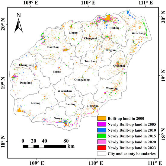
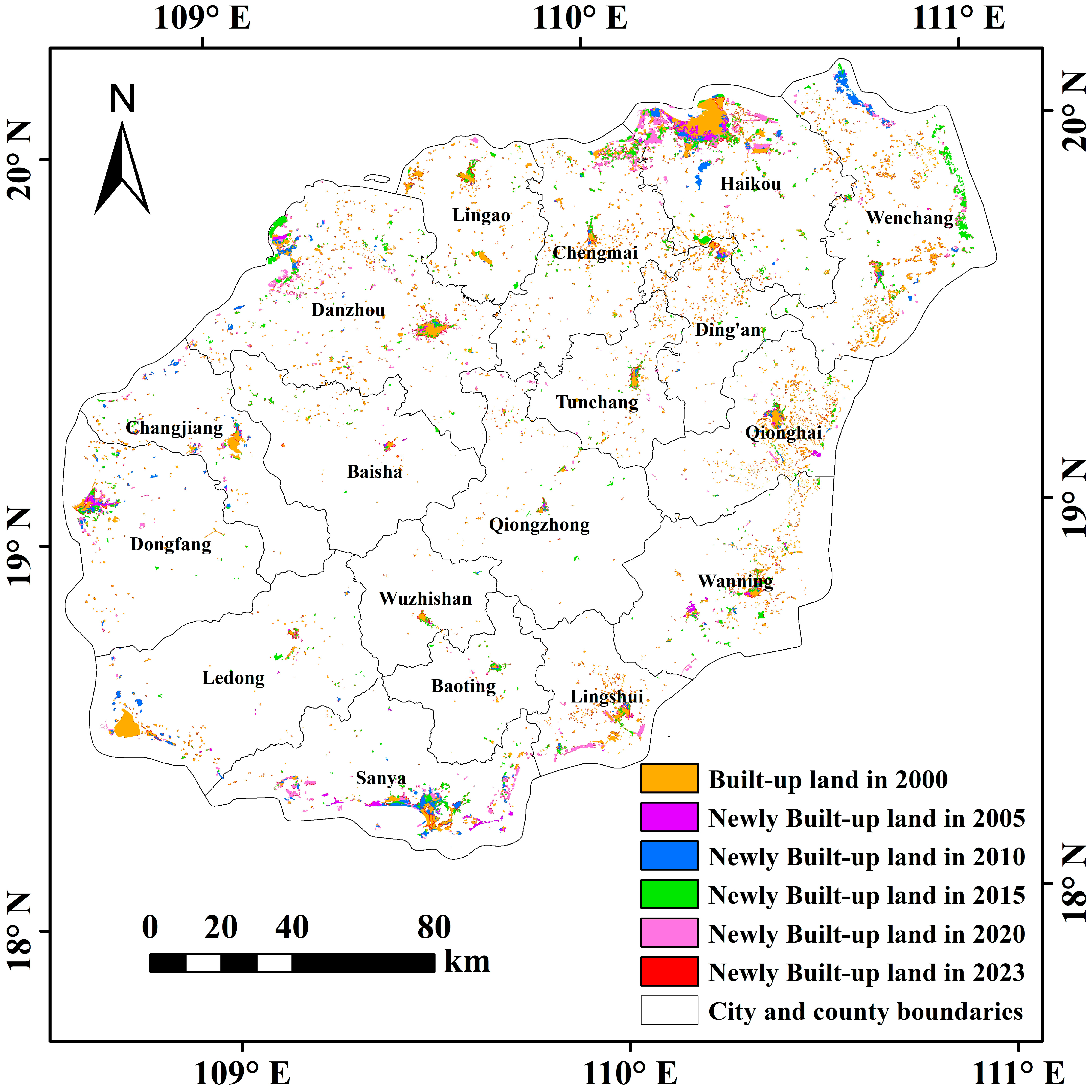
At the county scale, differences in land development pressure and estimated LUCEs were observed between coastal and interior areas. As shown in Figure 10, newly added built-up land from 2000 to 2023 was concentrated mainly in Haikou, Sanya, and parts of the eastern coast, and these areas largely overlapped with high-LUCE zones. Danzhou and Changjiang also maintained relatively high LUCEs, which was consistent with the concentration of industrial activities in the western part of the island [71,72].

Figure 10. Spatial characteristics of built-up land expansion.

These spatial differences indicate that ecological function areas and development-oriented counties play different roles in regional carbon management. The central ecological counties maintain extensive ecological land and relatively low estimated LUCEs under long-term conservation, whereas coastal and industrial counties account for a larger proportion of regional emissions because of concentrated urban development and economic activity [23,73]. In this context, structural adjustment of LULCC should consider differences in regional land use functions, emission control pressures, and ecological conservation responsibilities.

The observed spatial heterogeneity in built-up land expansion and estimated LUCEs indicates substantial differences among counties in development intensity and carbon-emission patterns. Coastal and western development areas experienced faster LUCE growth, whereas the forest-dominated central region remained a comparatively low-emission area. Accordingly, regional land use and carbon-management measures should account for differences in development intensity, land use structure, and designated ecological functions among counties.

4.3. Industrial Restructuring and LUCE Evolution Under the HFTP Context

The development of HFTP has occurred alongside substantial changes in the industrial structure of HI. By 2017, the tertiary sector accounted for 55.71% of regional GDP, and the negative list for industrial access implemented in 2019 further restricted the entry of high-energy-consuming, highly polluting, and high-emission industries. Tourism, modern services, high technology, and efficient agriculture have consequently become increasingly important components of the regional economy [74,75]. However, the relationship between these structural changes and estimated LUCE is not straightforward. The GeoDetector analysis showed relatively high q-values for the interactions of GDP with the proportions of tertiary and secondary industries. Because county-level energy-related emissions were allocated in proportion to GDP, GDP is partly embedded in the spatial distribution of estimated LUCEs. The observed GDP-related associations therefore contain both spatial covariation in economic and industrial characteristics and the structural dependence introduced by the allocation of indirect emissions.

The shift toward a service-oriented economy also coincided with continued carbon-emission pressures associated with transportation, construction, tourism, and infrastructure-related activities. Previous studies on HI reported that transportation-sector carbon emissions increased and subsequently stabilized between 2006 and 2020, while the corresponding decoupling relationship remained variable [76]. At a broader scale, the global tourism carbon footprint has continued to increase because growth in tourism demand has outpaced improvements in carbon efficiency, with transportation accounting for an important share of tourism-related emissions [77]. Comparable variability has also been reported in Malta, where the degree of decoupling between economic growth and environmental pressures differed among environmental indicators and accounting boundaries [78]. These studies indicate that an increasing share of tertiary activities does not necessarily correspond to a proportional reduction in emission pressure, particularly where service sector growth is accompanied by substantial transportation, construction, and infrastructure demand.

Industrial restructuring on HI coincided with continued LUCE growth rather than a uniform decline. The expansion of the tertiary sector occurred alongside persistent land development and energy-related emission pressures, while LMU–LUCE decoupling states varied across periods and administrative units. These patterns indicate that the evolution of LUCEs cannot be characterized by changes in sectoral composition alone and is also associated with the land and energy use demands accompanying different development activities.

4.4. Limitations and Prospects

This study has several limitations. First, LUCE accounting relied on literature-based fixed carbon coefficients assigned to broad land use categories. This approach was adopted to maintain a consistent accounting boundary and comparability across administrative units and study years. It follows the general IPCC accounting logic of combining activity data with the corresponding emission or removal factors, and the broad land use categories are generally comparable to the major land classes represented in the IPCC framework [46,79]. However, the approach does not constitute a complete IPCC Agriculture, Forestry and Other Land Use inventory. Because a single coefficient was assigned to forestland, within-category differences in forest age, biomass density, degradation, management, and associated carbon removals were not represented explicitly; these characteristics were not analyzed separately in this study. Higher-tier IPCC approaches would require repeated and spatially explicit information on land use transitions and carbon-stock changes that were not consistently available for all counties and study years. Applying such methods only to selected years or administrative units would have reduced temporal and spatial comparability. The resulting estimates should therefore be interpreted as coefficient-based approximations for comparing regional temporal and spatial patterns, rather than as direct measurements of ecosystem carbon sequestration or IPCC Tier 2 or Tier 3 inventory estimates [80,81]. Their application to other regions would require locally appropriate activity data and emission or sequestration coefficients. Future studies could improve accounting by adopting locally calibrated and temporally variable coefficients where consistent data are available.

Second, the analysis was constrained by data availability. Because consistent city- and county-level energy consumption data were unavailable for the entire study period, GDP was used to spatially allocate indirect carbon emissions. The GDP-based allocation may not fully capture county-level heterogeneity in sectoral composition, energy intensity, and fuel mix, thereby introducing uncertainty into the estimated spatial distribution of LUCEs [47,48]. Because harmonized county-level energy consumption data and parameter-specific uncertainty information were unavailable for the full study period, the magnitude of this potential bias could not be quantified empirically. Accordingly, the county-level estimates are more appropriate for characterizing broad spatial patterns than for resolving small differences among administrative units with similar values. Moreover, because GDP was also included in the factor analysis, the estimated association between GDP and LUCE may partly reflect the GDP-based allocation structure. Future studies could incorporate more detailed sectoral energy consumption data to improve county-level emission estimates.

Third, the analysis was conducted within the specific geographic, ecological, and development context of HI. The absence of systematic comparisons with mainland coastal regions and other islands limits the broader validation of the identified LUCE patterns and factor associations. Future studies should therefore test the analytical framework across regions with different development stages, economic structures, and ecological conditions and develop scenario-based coupling models linking LULCC, carbon emissions, and socioeconomic systems. Incorporating ecosystem service flow perspectives may further clarify the spatial support relationships between carbon sink and high-emission areas and provide a basis for carbon quota allocation and ecological compensation [82].

5. Conclusions

This study examined spatiotemporal evolution, driving associations, and decoupling characteristics of LUCE on HI from 2000 to 2023. The results show that estimated total LUCEs on HI increased from approximately 201.41 × 10⁴ t in 2000 to 1443.54 × 10⁴ t in 2023, mainly because of the growth of the carbon source component. During the same period, the carbon sink offset ratio decreased from 40.45% to 8.84%, indicating that estimated carbon sinks compensated for a progressively smaller proportion of carbon source emissions. Spatially, LUCEs remained higher in northern and coastal development areas and lower in the forest-dominated central and interior counties. The LUCE centroid gradually shifted from the northeastern part of the island toward the interior, accompanied by an expansion of its spatial distribution. At the county level, Haikou consistently recorded the highest estimated LUCEs, whereas Qiongzhong, Baisha, and Wuzhishan remained at comparatively low levels. The exploratory GWR and GeoDetector analyses further showed that the relationships between LUCEs and the selected natural and socioeconomic factors varied across administrative units. GDP, built-up land proportion, and industrial structure exhibited relatively high explanatory power in several years, while combinations of socioeconomic and land use factors generally showed greater explanatory power for LUCE spatial differentiation than the corresponding individual factors. However, because GDP was used to allocate county-level indirect emissions, GDP-related associations partly reflect the accounting structure. LMU–LUCE decoupling states also varied across administrative units and development periods, with relatively favorable states occurring more frequently in several central ecological counties, whereas negative decoupling persisted or re-emerged in some development-oriented coastal areas. These spatial differences underscore the importance of accounting for heterogeneity in development intensity, land use structure, and ecological land configuration in regional land use and carbon management.

References

- Hong, C.; Burney, J.A.; Pongratz, J.; Nabel, J.E.M.S.; Mueller, N.D.; Jackson, R.B.; Davis, S.J. Global and regional drivers of land-use emissions in 1961–2017. Nature 2021, 589, 554–561. [Google Scholar] [CrossRef] [Scilit] [PubMed]
- Houghton, R.A.; House, J.I.; Pongratz, J.; Van Der Werf, G.R.; Defries, R.S.; Hansen, M.C.; Le Quéré, C.; Ramankutty, N. Carbon emissions from land use and land-cover change. Biogeosciences 2012, 9, 5125–5142. [Google Scholar] [CrossRef] [Scilit]
- Wang, J.; Feng, L.; Palmer, P.I.; Liu, Y.; Fang, S.; Bösch, H.; O’Dell, C.W.; Tang, X.; Yang, D.; Liu, L.; et al. Large Chinese land carbon sink estimated from atmospheric carbon dioxide data. Nature 2020, 586, 720–723. [Google Scholar] [CrossRef] [Scilit] [PubMed]
- Gidden, M.J.; Gasser, T.; Grassi, G.; Forsell, N.; Janssens, I.; Lamb, W.F.; Minx, J.; Nicholls, Z.; Steinhauser, J.; Riahi, K. Aligning climate scenarios to emissions inventories shifts global benchmarks. Nature 2023, 624, 102–108. [Google Scholar] [CrossRef] [Scilit] [PubMed]
- Rong, T.; Zhang, P.; Zhu, H.; Jiang, L.; Li, Y.; Liu, Z. Spatial correlation evolution and prediction scenario of land use carbon emissions in China. Ecol. Inform. 2022, 71, 101802. [Google Scholar] [CrossRef] [Scilit]
- Zhang, S.; Chen, W.; Zhang, Q.; Krey, V.; Byers, E.; Rafaj, P.; Nguyen, B.; Awais, M.; Riahi, K. Targeting net-zero emissions while advancing other sustainable development goals in China. Nat. Sustain. 2024, 7, 1107–1119. [Google Scholar] [CrossRef] [Scilit]
- Harper, A.B.; Powell, T.; Cox, P.M.; House, J.; Huntingford, C.; Lenton, T.M.; Sitch, S.; Burke, E.; Chadburn, S.E.; Collins, W.J.; et al. Land-use emissions play a critical role in land-based mitigation for Paris climate targets. Nat. Commun. 2018, 9, 2938. [Google Scholar] [CrossRef] [Scilit] [PubMed]
- van Soest, H.L.; den Elzen, M.G.J.; van Vuuren, D.P. Net-zero emission targets for major emitting countries consistent with the Paris Agreement. Nat. Commun. 2021, 12, 2140. [Google Scholar] [CrossRef] [Scilit] [PubMed]
- Han, J.; Hu, Z.; Wang, P.; Yan, Z.; Li, G.; Zhang, Y.; Zhou, T. Spatio-temporal evolution and optimization analysis of ecosystem service value—A case study of coal resource-based city group in Shandong, China. J. Clean. Prod. 2022, 363, 132602. [Google Scholar] [CrossRef] [Scilit]
- Tong, X.; Brandt, M.; Yue, Y.; Ciais, P.; Rudbeck Jepsen, M.; Penuelas, J.; Wigneron, J.-P.; Xiao, X.; Song, X.-P.; Horion, S.; et al. Forest management in southern China generates short term extensive carbon sequestration. Nat. Commun. 2020, 11, 129. [Google Scholar] [CrossRef] [Scilit] [PubMed]
- Mao, S.; Mao, M.; Gong, W.; Chen, Y.; Ma, Y.; Chen, R.; Wang, M.; Zhang, X.; Xu, J.; Jia, J.; et al. Assessing Anthropogenic Impacts on the Carbon Sink Dynamics in Tropical Lowland Rainforest Using Multiple Remote Sensing Data: A Case Study of Jianfengling, China. Forests 2025, 16, 1611. [Google Scholar] [CrossRef] [Scilit]
- Wu, T.; Chen, Z.; Chen, Y.; Chen, Y.; Lei, J.; Chen, X.; Li, Y.; Pan, X. Biomass Characteristics of Tropical Montane Rain Forest in National Park of Hainan Tropical Rainforest. Land 2025, 14, 608. [Google Scholar] [CrossRef] [Scilit]
- Lei, J.; Zhang, L.; Chen, Z.; Wu, T.; Chen, X.; Li, Y. The impact of land use change on carbon storage and multi-scenario prediction in Hainan Island using InVEST and CA-Markov models. Front. For. Glob. Change 2024, 7, 1349057. [Google Scholar] [CrossRef] [Scilit]
- Zhang, X.; Fan, H.; Hou, H.; Xu, C.; Sun, L.; Li, Q.; Ren, J. Spatiotemporal evolution and multi-scale coupling effects of land-use carbon emissions and ecological environmental quality. Sci. Total Environ. 2024, 922, 171149. [Google Scholar] [CrossRef] [Scilit] [PubMed]
- Ai, J.; Yu, K.; Zeng, Z.; Yang, L.; Liu, Y.; Liu, J. Assessing the dynamic landscape ecological risk and its driving forces in an island city based on optimal spatial scales: Haitan Island, China. Ecol. Indic. 2022, 137, 108771. [Google Scholar] [CrossRef] [Scilit]
- Pan, Y.; Zhai, M.; Lin, L.; Lin, Y.; Cai, J.; Deng, J.-S.; Wang, K. Characterizing the spatiotemporal evolutions and impact of rapid urbanization on island sustainable development. Habitat Int. 2016, 53, 215–227. [Google Scholar] [CrossRef] [Scilit]
- Chi, Y.; Shi, H.; Wang, Y.; Guo, Z.; Wang, E. Evaluation on island ecological vulnerability and its spatial heterogeneity. Mar. Pollut. Bull. 2017, 125, 216–241. [Google Scholar] [CrossRef] [Scilit] [PubMed]
- Tuholske, C.; Tane, Z.; López-Carr, D.; Roberts, D.; Cassels, S. Thirty years of land use/cover change in the Caribbean: Assessing the relationship between urbanization and mangrove loss in Roatán, Honduras. Appl. Geogr. 2017, 88, 84–93. [Google Scholar] [CrossRef] [Scilit]
- Steibl, S.; Franke, J.; Laforsch, C. Tourism and urban development as drivers for invertebrate diversity loss on tropical islands. R. Soc. Open Sci. 2021, 8, 210411. [Google Scholar] [CrossRef] [Scilit] [PubMed]
- Gong, W.; Duan, X.; Sun, Y.; Zhang, Y.; Ji, P.; Tong, X.; Qiu, Z.; Liu, T. Multi-scenario simulation of land use/cover change and carbon storage assessment in Hainan coastal zone from perspective of free trade port construction. J. Clean. Prod. 2023, 385, 135630. [Google Scholar] [CrossRef] [Scilit]
- Lei, J.; Chen, Y.; Li, L.; Chen, Z.; Chen, X.; Wu, T.; Li, Y. Spatiotemporal change of habitat quality in Hainan Island of China based on changes in land use. Ecol. Indic. 2022, 145, 109707. [Google Scholar] [CrossRef] [Scilit]
- Ma, Y.; Mao, M.; Xie, Z.; Mao, S.; Wang, Y.; Chen, Y.; Xu, J.; Liu, T.; Gong, W.; Wu, L. Spatiotemporal Dynamics and Simulation of Landscape Ecological Risk and Ecological Zoning Under the Construction of Free Trade Pilot Zones: A Case Study of Hainan Island, China. Land 2025, 14, 940. [Google Scholar] [CrossRef] [Scilit]
- Cai, Y.; Su, S.; Zhang, P.; Chen, M.; Wang, Y.; Xie, Y.; Tan, Q. Quantifying high-resolution carbon emissions driven by land use change in the Guangdong-Hong Kong-Macao Greater Bay Area. Urban Clim. 2024, 55, 101943. [Google Scholar] [CrossRef] [Scilit]
- Zhao, J.; Xu, S.; Ren, Y.; Tang, X. A breakthrough land-use-based carbon accounting framework for multi-scale evaluation: Coupling optimization algorithm and LCA. Sustain. Cities Soc. 2025, 120, 106132. [Google Scholar] [CrossRef] [Scilit]
- Song, M.; Zhang, L.; Gao, Y.; Li, E. Spatiotemporal evolution and influence mechanism of the carbon footprint of energy consumption at county level in the Yellow River Basin. Sci. Total Environ. 2023, 883, 163710. [Google Scholar] [CrossRef] [Scilit] [PubMed]
- Sun, H.; Liang, H.; Chang, X.; Cui, Q.; Tao, Y. Land Use Patterns on Carbon Emission and Spatial Association in China. Econ. Geogr. 2015, 35, 154–162. [Google Scholar] [CrossRef]
- Liu, L.; Qu, J.; Gao, F.; Maraseni, T.N.; Wang, S.; Aryal, S.; Zhang, Z.; Wu, R. Land Use Carbon Emissions or Sink: Research Characteristics, Hotspots and Future Perspectives. Land 2024, 13, 279. [Google Scholar] [CrossRef] [Scilit]
- Zhu, C.; Zhang, X.; Zhou, M.; He, S.; Gan, M.; Yang, L.; Wang, K. Impacts of urbanization and landscape pattern on habitat quality using OLS and GWR models in Hangzhou, China. Ecol. Indic. 2020, 117, 106654. [Google Scholar] [CrossRef] [Scilit]
- Wu, H.; Deng, K.; Dong, Z.; Meng, X.; Zhang, L.; Jiang, S.; Yang, L.; Xu, Y. Comprehensive assessment of land use carbon emissions of a coal resource-based city, China. J. Clean. Prod. 2022, 379, 134706. [Google Scholar] [CrossRef] [Scilit]
- Chen, M.; Yan, Z.; Zhang, J.; Xue, Z. Analysis of Spatio-Temporal Dynamics and Determinants of Land Use Carbon Emissions in Jiangsu Province, China. Land 2025, 14, 905. [Google Scholar] [CrossRef] [Scilit]
- Zhou, Y.; Chen, M.; Tang, Z.; Mei, Z. Urbanization, land use change, and carbon emissions: Quantitative assessments for city-level carbon emissions in Beijing-Tianjin-Hebei region. Sustain. Cities Soc. 2021, 66, 102701. [Google Scholar] [CrossRef] [Scilit]
- Zhang, Z.; Jin, G. Spatiotemporal differentiation of carbon budget and balance zoning: Insights from the middle reaches of the Yangtze River Urban Agglomeration, China. Appl. Geogr. 2024, 167, 103293. [Google Scholar] [CrossRef] [Scilit]
- Zhao, L.; Zhang, C.; Wang, Q.; Yang, C.; Zhou, W. Spatio-temporal variations of land use carbon emissions and its low carbon strategies for coastal areas in China with nighttime lighting data. J. Environ. Manag. 2025, 385, 125651. [Google Scholar] [CrossRef] [Scilit] [PubMed]
- Lei, J.; Chen, Z.; Chen, X.; Li, Y.; Wu, T. Spatio-temporal changes of land use and ecosystem services value in Hainan Island from 1980 to 2018. Acta Ecol. Sin. 2020, 40, 4760–4773. [Google Scholar]
- Lai, J.; Qi, S.; Chen, J.; Guo, J.; Wu, H.; Chen, Y. Exploring the spatiotemporal variation of carbon storage on Hainan Island and its driving factors: Insights from InVEST, FLUS models, and machine learning. Ecol. Indic. 2025, 172, 113236. [Google Scholar] [CrossRef] [Scilit]
- Zhang, L.; Zhang, Y.; Ma, W.; Zhang, H.; Deng, Y.; Wang, M.; Wang, W. Conservation implications of mismatched diversity between mangrove plants and benthic mollusks. J. Environ. Manag. 2025, 384, 125505. [Google Scholar] [CrossRef] [Scilit] [PubMed]
- Wei, L.; Li, M.; Ma, Y.; Wang, Y.; Wu, G.; Liu, T.; Gong, W.; Mao, M.; Zhao, Y.; Wei, Y.; et al. Construction of an Ecological Security Pattern for the National Park of Hainan Tropical Rainforest on the Basis of the Importance of the Function and Sensitivity of Its Ecosystem Services. Land 2024, 13, 1618. [Google Scholar] [CrossRef] [Scilit]
- Chen, H.; Li, D.; Chen, Y.; Zhao, Z. Spatial–Temporal Evolution Monitoring and Ecological Risk Assessment of Coastal Wetlands on Hainan Island, China. Remote Sens. 2023, 15, 1035. [Google Scholar] [CrossRef] [Scilit]
- Xu, Z.; Li, C.; Lu, N. Decoupling Relationship Between Land Mixed Use and Carbon Emissions in Hohhot-Baotou-Ordos-Yulin Urban Agglomeration. Res. Environ. Sci. 2022, 35, 299–308. [Google Scholar] [CrossRef]
- Paustian, K.; Ravindranath, N.; Van Amstel, A. 2006 IPCC Guidelines for National Greenhouse Gas Inventories; Volume 4 Agriculture, Forestry and Other Land Use; Institute for Global Environmental Strategies: Hayama, Japan, 2006. [Google Scholar]
- Sun, Y.; Mao, D.; Qiu, D. Spatial and temporal analysis and multi-scenario simulation of land use carbon emissions in Changsha City. J. Agric. Resour. Environ. 2025, 42, 529–542. [Google Scholar] [CrossRef]
- Chen, J.; Zhang, J.; Li, J.; Li, S. Spatio-temporal pattern of carbon emissions and its driving factors in the Beijing-Tianjin-Hebei region. Acta Ecol. Sin. 2024, 44, 2270–2283. [Google Scholar] [CrossRef]
- Li, Z.; Zhou, D.; Jiang, J.; Ma, J.; Zhu, X.; Shi, P.; Zhang, J.; Dong, Q. Spatial and Temporal Evolution Characteristics of Carbon Emission from Land Use and Influencing Factors in Gansu Province. Environ. Sci. 2024, 45, 5040–5048. [Google Scholar] [CrossRef] [Scilit] [PubMed]
- Lv, Q.; Zhang, L.; Luo, Y. Spatial-temporal Pattern and Carbon Balance Zoning of County Land Use Carbon Emissions in the Yellow River Basin. Environ. Sci. 2025, 46, 6209–6220. [Google Scholar] [CrossRef] [Scilit] [PubMed]
- Deng, Y.; Chen, H.; Hai, Y.; Zhou, J.; Jize, D.; Luo, J.; Li, L. Spatial Patterns of Carbon Emission from Land Use and Carbon Balance Partitioning in Chengdu-Chongqing Economic Zone. Bull. Soil Water Conserv. 2024, 44, 337–346. [Google Scholar] [CrossRef]
- Zhang, C.-Y.; Zhao, L.; Zhang, H.; Chen, M.-N.; Fang, R.-Y.; Yao, Y.; Zhang, Q.-P.; Wang, Q. Spatial-temporal characteristics of carbon emissions from land use change in Yellow River Delta region, China. Ecol. Indic. 2022, 136, 108623. [Google Scholar] [CrossRef] [Scilit]
- Liu, W.; Zhang, X.; Zhu, Y.; Li, X.; Jin, L.; Hu, S. Analyzing Integrated Carbon Emissions from Regional Transport and Land Use in the Context of National Spatial Planning. Sustainability 2025, 17, 7873. [Google Scholar] [CrossRef] [Scilit]
- Liu, C.; Xu, R.; Xu, K.; Lin, Y.; Cao, Y. Carbon Emission Effects of Land Use in Chaobai River Region of Beijing–Tianjin–Hebei, China. Land 2023, 12, 1168. [Google Scholar] [CrossRef] [Scilit]
- Li, W.; Wang, K.; Liu, H.; Zhang, Y.; Zhu, X. Construction Land Transfer Scale and Carbon Emission Intensity: Empirical Evidence Based on County-Level Land Transactions in Jiangsu Province, China. Land 2024, 13, 917. [Google Scholar] [CrossRef] [Scilit]
- Lefever, D.W. Measuring Geographic Concentration by Means of the Standard Deviational Ellipse. Am. J. Sociol. 1926, 32, 88–94. [Google Scholar] [CrossRef] [Scilit] [PubMed]
- Zhao, L.; Zhao, Z. Projecting the Spatial Variation of Economic Based on the Specific Ellipses in China. Sci. Geogr. Sin. 2014, 34, 979–986. [Google Scholar] [CrossRef]
- Yuan, L.; Chai, L.; He, W.; Kong, Y.; Qi, Y. Carbon Footprint Assessment and Analysis on Driving Factor in North China from the Perspective of Spatial and Temporal Heterogeneity. Ecol. Econ. 2025, 41, 70–79. [Google Scholar]
- Brunsdon, C.; Fotheringham, A.S.; Charlton, M.E. Geographically Weighted Regression: A Method for Exploring Spatial Nonstationarity. Geogr. Anal. 1996, 28, 281–298. [Google Scholar] [CrossRef] [Scilit]
- Liu, C.; Wu, X.; Wang, L. Analysis on land ecological security change and affect factors using RS and GWR in the Danjiangkou Reservoir area, China. Appl. Geogr. 2019, 105, 1–14. [Google Scholar] [CrossRef] [Scilit]
- Dadashpoor, H.; Azizi, P.; Moghadasi, M. Land use change, urbanization, and change in landscape pattern in a metropolitan area. Sci. Total Environ. 2019, 655, 707–719. [Google Scholar] [CrossRef] [Scilit] [PubMed]
- Wang, J.-F.; Zhang, T.-L.; Fu, B.-J. A measure of spatial stratified heterogeneity. Ecol. Indic. 2016, 67, 250–256. [Google Scholar] [CrossRef] [Scilit]
- Ma, G.; Lu, R.; Wu, B. Spatio-temporal Evolution Characteristics and Driving Mechanism of Land Use Carbon Emission at County Level in Guangxi. Chin. J. Agric. Resour. Reg. Plan. 2025, 11, 153–166. [Google Scholar]
- Wang, W.; Yang, S.; Hai, Y. The spatiotemporal evolution and influencing factors of carbon emissions from land use in Ningxia. Arid Zone Res. 2025, 42, 545–555. [Google Scholar] [CrossRef]
- Li, D.; Yang, Y.; Xia, F.; Sun, W.; Li, X.; Xie, Y. Exploring the influences of different processes of habitat fragmentation on ecosystem services. Landsc. Urban Plan. 2022, 227, 104544. [Google Scholar] [CrossRef] [Scilit]
- Tapio, P. Towards a theory of decoupling: Degrees of decoupling in the EU and the case of road traffic in Finland between 1970 and 2001. Transp. Policy 2005, 12, 137–151. [Google Scholar] [CrossRef] [Scilit]
- Cui, L.; Wang, F.; Zhang, H.; Zhao, H.; Shi, J. Accounting for carbon emissions in social water cycle system in nine provinces along the yellow river and analysis of influencing factors. Carbon Balance Manag. 2024, 19, 33. [Google Scholar] [CrossRef] [Scilit] [PubMed]
- Zhang, Y.; Song, W.; Fu, S.; Yang, D. Decoupling of Land Use Intensity and Ecological Environment in Gansu Province, China. Sustainability 2020, 12, 2779. [Google Scholar] [CrossRef] [Scilit]
- Seto, K.C.; Güneralp, B.; Hutyra, L.R. Global forecasts of urban expansion to 2030 and direct impacts on biodiversity and carbon pools. Proc. Natl. Acad. Sci. USA 2012, 109, 16083–16088. [Google Scholar] [CrossRef] [Scilit] [PubMed]
- Ingrisch, J.; Bahn, M. Towards a Comparable Quantification of Resilience. Trends Ecol. Evol. 2018, 33, 251–259. [Google Scholar] [CrossRef] [Scilit] [PubMed]
- Yao, Y.; Liu, Y.; Fu, F.; Song, J.; Wang, Y.; Han, Y.; Wu, T.; Fu, B. Declined terrestrial ecosystem resilience. Glob. Change Biol. 2024, 30, e17291. [Google Scholar] [CrossRef] [Scilit] [PubMed]
- Zhu, C.; Fan, W.; Wu, X.; Zhang, Z.; Chen, Y. Spatial mismatch and the attribution analysis of carbon storage demand and supply in the Yangtze River Economic Belt, China. J. Clean. Prod. 2024, 434, 140036. [Google Scholar] [CrossRef] [Scilit]
- Guo, P.; Zhao, X.; Shi, J.; Huang, J.; Tang, J.; Zhang, R.; Chen, J.; Wang, Q.; Zeng, J. The influence of temperature and precipitation on the vegetation dynamics of the tropical island of Hainan. Theor. Appl. Climatol. 2021, 143, 429–445. [Google Scholar] [CrossRef] [Scilit]
- Yao, X.; Zhou, L.; Wu, T.; Yang, X.; Ren, M. Ecosystem services in National Park of Hainan Tropical Rainforest of China: Spatiotemporal dynamics and conservation implications. J. Nat. Conserv. 2024, 80, 126649. [Google Scholar] [CrossRef] [Scilit]
- Meng, Y.; Gou, R.; Bai, J.; Moreno-Mateos, D.; Davis, C.C.; Wan, L.; Song, S.; Zhang, H.; Zhu, X.; Lin, G. Spatial patterns and driving factors of carbon stocks in mangrove forests on Hainan Island, China. Glob. Ecol. Biogeogr. 2022, 31, 1692–1706. [Google Scholar] [CrossRef] [Scilit]
- Li, Z.; Liu, L.; Sun, C.; Shan, X.; Zhao, H. Spatio-temporal variation and drivers of blue carbon sequestration in Hainan Island, China. Mar. Environ. Res. 2024, 197, 106476. [Google Scholar] [CrossRef] [Scilit] [PubMed]
- Guo, Q.; Ma, M.; Cheng, Y. Spatio-temporal Characteristic of Urban-Rural Integration Development Level in Hainan Free Trade Port and Its Driving Mechanism. Econ. Geogr. 2024, 44, 62–71. [Google Scholar] [CrossRef]
- Geng, J.; Yuan, M.; Xu, S.; Bai, T.; Xiao, Y.; Li, X.; Xu, D. Urban Expansion Was the Main Driving Force for the Decline in Ecosystem Services in Hainan Island during 1980–2015. Int. J. Environ. Res. Public Health 2022, 19, 15665. [Google Scholar] [CrossRef] [Scilit] [PubMed]
- Cumming, G.S. Protected area management has significant spillover effects on vegetation. Nature 2026, 650, 642–651. [Google Scholar] [CrossRef] [Scilit] [PubMed]
- Xiu, C.; Li, T. Construction of the Hainan Free Trade Port from the perspective of regional cultural development. Front. Earth Sci. 2023, 10, 1032953. [Google Scholar] [CrossRef] [Scilit]
- Zhong, C.; Wu, X.; Jia, P.; Zhang, K. Study on the coupling coordination effect and dynamic relationship between tourism development and the ecological environment: A case study of Hainan Island. Front. Ecol. Evol. 2024, 12, 1284278. [Google Scholar] [CrossRef] [Scilit]
- Tang, Y.; Jiang, H.; Yang, X.; Zhang, D. Decoupling Effect and Influencing Factors of Transportation Carbon Emissions in Hainan Province. IEEE Access 2024, 12, 131750–131761. [Google Scholar] [CrossRef] [Scilit]
- Lenzen, M.; Sun, Y.-Y.; Faturay, F.; Ting, Y.-P.; Geschke, A.; Malik, A. The carbon footprint of global tourism. Nat. Clim. Change 2018, 8, 522–528. [Google Scholar] [CrossRef] [Scilit]
- Conrad, E.; Cassar, L.F. Decoupling Economic Growth and Environmental Degradation: Reviewing Progress to Date in the Small Island State of Malta. Sustainability 2014, 6, 6729–6750. [Google Scholar] [CrossRef] [Scilit]
- Sun, Y.; Zhi, J.; Han, C.; Xue, C.; Zhao, W.; Liu, W.; Bao, S. The Impact of Future Land Use Change on Carbon Emission and Its Optimization Strategy. Forests 2024, 15, 1292. [Google Scholar] [CrossRef] [Scilit]
- Peng, D.; Zhang, B.; Zheng, S.; Ju, W.; Chen, J.M.; Ciais, P.; Guo, H.; Pan, Y.; Yu, L.; Xu, Y.; et al. Newly established forests dominated global carbon sequestration change induced by land cover conversions. Nat. Commun. 2025, 16, 6570. [Google Scholar] [CrossRef] [Scilit] [PubMed]
- Mo, L.; Zohner, C.M.; Reich, P.B.; Liang, J.; de Miguel, S.; Nabuurs, G.-J.; Renner, S.S.; van den Hoogen, J.; Araza, A.; Herold, M.; et al. Integrated global assessment of the natural forest carbon potential. Nature 2023, 624, 92–101. [Google Scholar] [CrossRef] [Scilit] [PubMed]
- Wu, C.; Lu, R.; Zhang, P.; Dai, E. Multilevel ecological compensation policy design based on ecosystem service flow: A case study of carbon sequestration services in the Qinghai-Tibet Plateau. Sci. Total Environ. 2024, 921, 171093. [Google Scholar] [CrossRef] [Scilit] [PubMed]
Disclaimer/Publisher’s Note: The statements, opinions and data contained in all publications are solely those of the individual author(s) and contributor(s) and not of MDPI and/or the editor(s). MDPI and/or the editor(s) disclaim responsibility for any injury to people or property resulting from any ideas, methods, instructions or products referred to in the content. |
© 2026 by the authors. Licensee MDPI, Basel, Switzerland. This article is an open access article distributed under the terms and conditions of the Creative Commons Attribution (CC BY) license.