Landslide Susceptibility Assessment in the Upper Minjiang River: A Random Forest Approach Based on Slope Unit

Abstract

In a high-mountain gorge region, landslide hazards pose a serious threat to the upper Minjiang River, located at the eastern edge of the Tibetan Plateau. To map susceptibility in the upper Minjiang River basin, this study used a Random Forest model in conjunction with slope unit subdivisions. First, a landslide inventory containing 3785 landslides was established using human–machine interactive interpretation techniques. After a multicollinearity analysis, 11 key conditioning factors were selected to construct a spatial database, including elevation, slope, aspect, curvature, topographic wetness index, stream power index, distance to fault, peak ground acceleration, distance to road, vegetation index, and rainfall. The r.slopeunits algorithm was implemented to partition the study area into discrete slope units. The ideal parameter combination for slope units was determined through integrating the normalized slope aspect standard deviation and Moran’s I using an equal-weight scheme. Ultimately, 30,513 slope units were delineated in the upper Minjiang River. The random forest model trained on these ideal slope units was validated using a 70/30 split of landslide and non-landslide samples. In receiver operating characteristic (ROC) curve analysis, the model demonstrated excellent performance, with an area under the curve (AUC) of 0.852. The results indicate that small-scale landslides dominate the inventory in terms of frequency. Despite accounting for only 30% of the study area, the Very High and High susceptibility zones exhibit considerable degree of spatial overlap with current landslide clusters. Furthermore, shapley additive explanations (SHAP) explanatory metrics indicate that the random forest model’s predictive behavior is primarily influenced by terrain elevation, precipitation patterns, and proximity to transportation networks.

1. Introduction

Landslides are widespread globally and severely damage infrastructure and human settlements [1,2], leading to large-scale population migration and the abandonment of settlements [3,4]. High-altitude tectonic activity and drastic climate change within mountainous terrains are driving a persistent escalation in both the recurrence and magnitude of these geohazards [5]. The interplay of multiple natural factors and human activities makes risk identification more difficult [6]. Therefore, establishing a reliable assessment system is essential for disaster prevention and spatial planning.

Landslide susceptibility maps (LSMs) represent a fundamental prerequisite for the comprehensive evaluation and mitigation of landslide-related risks. This work relies on past landslide locations and environmental characteristics data. Using these spatial datasets, investigators can forecast the probability of slope failure across specific geographical regions [7,8]. Existing landslide susceptibility assessment methods include the analytic hierarchy process (AHP), frequency ratio method [9], information content method, expert scoring method, weighted evidence method, coefficient of determination method, fuzzy comprehensive evaluation method [10], and machine learning method [11,12]. The rapid development of remote sensing data and computing technology has enabled landslide susceptibility assessment methods to evolve from early qualitative assessments to machine learning methods centered on artificial intelligence [13,14,15]. These models excel at handling complex nonlinear relationships. They can handle high-dimensional data and demonstrate strong generalization capabilities. Random forests (RF) are a type of ensemble learning algorithm [16]. This algorithm has strong predictive performance. It can assign importance scores to different factors and has demonstrated satisfactory performance in geological hazard modeling tasks. For example, Li and Lan [17] reported average AUC values of 0.6808 for SU (Logistic Regression) and 0.6889 for SU (Neural Networks) in a slope-unit-based case study; Chang et al. [18] compared Random Forests (RF) with Multi-Layer Perceptron (MLP) in a slope unit framework and reported AUC values of 0.827 for Slope-RF and 0.805 for Slope-MLP, indicating better performance of the RF-based model in their case study. Huang et al. [19] showed that RF performance can vary with slope unit configuration, with the best scheme achieving an accuracy of 0.812, a precision of 0.807, and a recall of 0.818. These studies suggest that RF is a robust and competitive method in slope-unit-based landslide susceptibility assessment.

The reliability of landslide susceptibility modeling depends not only on the computational approach but also on the definition of assessment units. Evaluation units serve to represent the spatial framework for environmental factors and constitute the fundamental basis for sample construction and model training. Therefore, the definition of unit boundaries and their internal consistency can significantly affect model performance and final assessment results [20,21]. Two main types of evaluation units are commonly employed: grid units and slope units. Grid units are widely used to divide the study area into regular grids [22]. Slope units are terrain areas delineated by ridgelines and valley lines, representing hydrologically significant sub-basins. These units more accurately reflect natural slope boundaries and serve as the fundamental spatial units for landslide susceptibility assessment [23]. Evaluation results based on slope units better align with actual conditions and have demonstrated significant advantages in landslide susceptibility studies [24]. Research trends indicate that machine learning models based on slope cells offer significant advantages in improving the accuracy of landslide boundary identification and reducing spatial heterogeneity [25,26]. Despite the ongoing development of automatic slope cell division techniques supported by DEM, research on landslide susceptibility based on slope cells using machine learning remains limited, especially in high mountain and canyon areas with highly complex terrain.

Situated on the eastern periphery of the Tibetan Plateau, the upper Minjiang River lies in a seismically active region that is a global hotspot for frequent slope instabilities [27,28]. The terrain in this area has significant elevation differences, with many deep canyons [12]; the natural substrate is characterized by highly fractured lithology and a prolific fault network, which collectively compromise the structural integrity of the rock and soil masses. Affected by the environment and human activities, the upper Minjiang River has become a typical vulnerable area with frequent geological disaster chain activities, and it is urgent to carry out high-precision landslide susceptibility prediction.

A key scientific issue in slope-unit-based landslide susceptibility assessment is that the quality of the mapping unit itself can substantially affect the reliability of subsequent modeling results, especially in geomorphologically complex alpine canyon regions. However, previous studies have paid relatively limited attention to how slope unit delineation can be objectively optimized and to applying the optimized units to susceptibility modeling and interpretation in high mountain and canyon areas. This study focuses on the upper Minjiang River and constructs a multi-source factors database. Develops a landslide susceptibility assessment framework that combines slope unit optimization, a random forest model, and a SHAP-based interpretation method. The research content includes: (1) assembling a comprehensive historical landslide inventory derived from multi-source satellite imagery; (2) partitioning the upper Minjiang River basin into discrete slope units via the r.slopeunits algorithm; (3) selecting the ideal slope unit division results to construct an environmental factor database; (4) architecting a slope-unit-based Random Forest framework for susceptibility modeling; and (5) synthesizing the final susceptibility map while validating model efficacy through ROC/AUC metrics, confusion matrices, and F1-scores.

This study provides an integrated slope-unit-based modeling framework for landslide susceptibility assessment in the Upper Minjiang River, combining slope unit optimization, Random Forest modeling, and SHAP-based interpretation under the geomorphological conditions of a high mountain–canyon region, and offers vital scientific information for infrastructure planning, ecological preservation, and geohazard risk management throughout the seismically active eastern edge of the Tibetan Plateau.

2. Materials and Methods

2.1. Study Area

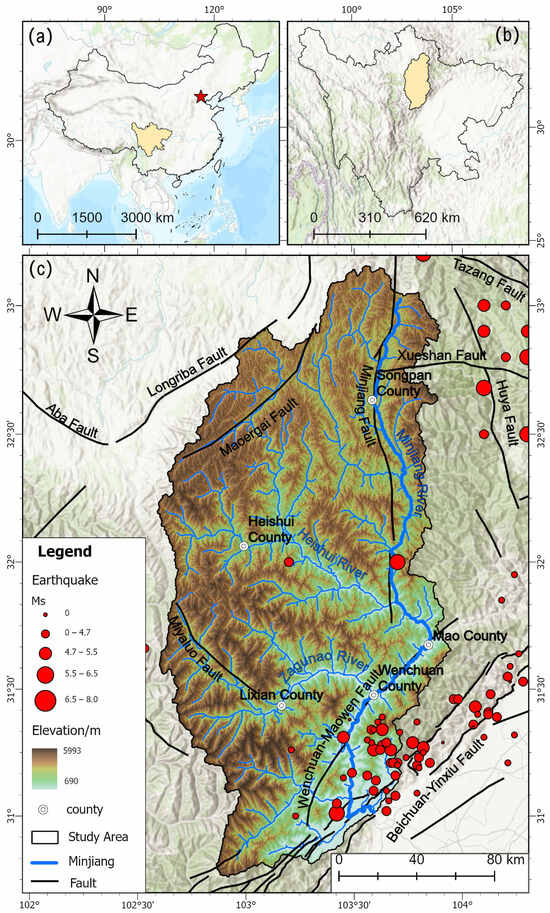
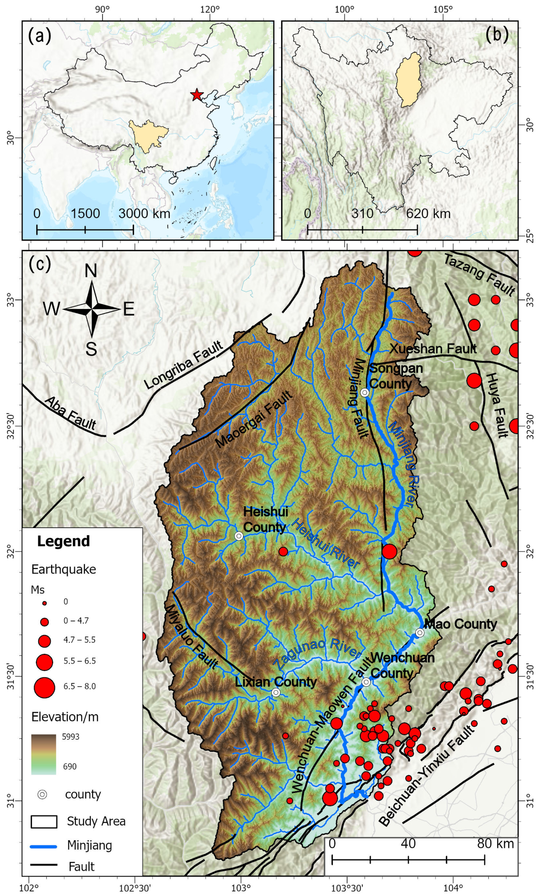
The upper Minjiang River is an important tributary of the Yangtze River Basin. It is a transitional area between the first and second steps of China, situated on the eastern side of the Tibetan Plateau. The study region spans a latitudinal range of 30°45′–33°9′ N and a longitudinal extent of 102°36′–104° E, covering an aggregate area of approximately 22,950 km². The terrain exhibits pronounced vertical relief, with elevations ranging from 690 to 5993 m and a mean altitude of 3389 m (Figure 1). This area is defined by rugged geomorphology, characterized by towering massifs intersected by incised canyons and constricted fluvial corridors. The climate is typical of a monsoon, with distinct dry and rainy seasons. The average annual rainfall is around 420 mm, concentrated in summer [29] and showing clear seasonality. During this period, landslides are a serious threat, and extreme rainfall events can easily induce rapid slope instability [30]. The environmental and climatic conditions of the study area are broadly consistent with the general trends observed across most regions of the Tibetan Plateau, characterized by rising temperatures, a general decrease in precipitation, and pronounced seasonal variability [31].

Figure 1. Geographical sketch of the area, highlighting the main faults and the epicentral locations of major historical earthquakes. (a) Map of China, with the red pentagram representing the capital, Beijing; (b) Map of Sichuan Province, China; (c) Study area.

Situated in China’s well-known North–South Seismic Belt, the upper Minjiang River region exhibits a complex and highly developed geological framework [32]. This region is marked by extensive tectonic deformation and robust fault systems. Specifically, the Songpan–Jiaochang seismic zone traverses the northern sector, while the Longmenshan seismic belt borders the southeastern margin, resulting in high-frequency seismic activity. Key structural features influencing this landscape include the Minjiang Fault, Xueshan Fault, Huya Fault, Yingxiu–Beichuan Fault, and Maoxian–Wenchuan Fault [33]. The area is severely affected by earthquake disasters [34,35,36,37], and earthquake-triggered landslides and secondary landslides after earthquake rainfall are widespread. According to historical earthquake records, the study area and its surroundings have experienced multiple strong earthquakes. The three largest earthquakes were the 7.5-magnitude Diexi earthquake in 1933 [36], the 7.2-magnitude Songpan earthquake in 1976 [37], and the 8.0-magnitude Wenchuan earthquake in 2008 [38].

2.2. Landslide Condition Factors

A total of sixteen conditioning factors were categorized into five distinct dimensions—topographical, lithological, hydro-meteorological, geomorphological, and anthropogenic—to serve as the primary drivers of landslide occurrence in this analysis. Detailed data sources for each factor are shown in Table 1. Six topographic factors were selected: elevation, slope, aspect, curvature, topographic relief index (TRI), and elevation coefficient of variation (ECV). For geology, lithology, peak ground acceleration (PGA), and distance to fault (Dis_fault) were selected. For meteorology and hydrology, the stream power index (SPI) and average annual rainfall were selected. The topographic wetness index (TWI), vegetation index (NDVI), and distance to river (Dis_river) were selected as environmental parameters. For human activities, land cover and distance to road (Dis_road) were selected.

Table 1. Statistics of research data sources.

	Factor	Type	Data Source	Spatial Resolution	Remark
Topography	Elevation	Continuous	Geospatial Data Cloud (https://www.gscloud.cn/)	12.5 m	Base DEM
	Slope	Continuous	Elevation Data Derivation	12.5 m	Derived from DEM
	Aspect	Categorical	Elevation Data Derivation	12.5 m	Derived from DEM
	Curvature	Continuous	Elevation Data Derivation	12.5 m	Derived from DEM
	TRI	Continuous	Elevation Data Derivation	12.5 m	Derived from DEM
	ECV	Continuous	Elevation Data Derivation	12.5 m	Derived from DEM
Geology	Lithology	Categorical	China Geological Survey (https://www.cgs.gov.cn/)		Official geological dataset
	PGA	Categorical	Seismic Motion Parameter Zoning Map of China (https://gb18306.net/oldmap, accessed on 16 June 2025)		Official seismic zonation dataset
	Dis_fault	Continuous	The China Active Faults Database (CAFD) (https://doi.org/10.12031/activefault.china.400.2023.db, accessed on 13 June 2025)	1:4,000,000	Vector fault data
Hydrology and meteorology	SPI	Continuous	Elevation Data Derivation	12.5 m	Derived from DEM
	Rainfall	Continuous	National Meteorological Information Centre (https://data.cma.cn/)	1000 m	Gridded rainfall dataset
	Dis_river	Continuous	National Catalogue Service For Geographic Information (https://www.webmap.cn/main.do?method=index, accessed on 13 June 2025)	1:1,000,000	Vector river data
Environment	TWI	Continuous	Elevation Data Derivation	12.5 m	Derived from DEM
	NDVI	Continuous	National Science & Technology Infrastructure (https://www.nesdc.org.cn/)	30 m	Remote sensing product
Human activity	Land Cover	Categorical	ESA WorldCover Consortium (https://esa-worldcover.org/en, accessed on 13 June 2025)	10 m	Global land cover product
	Dis_road	Continuous	National Catalogue Service for Geographic Information (https://www.webmap.cn/main.do?method=index, accessed on 13 June 2025)	1:1,000,000	Vector road data

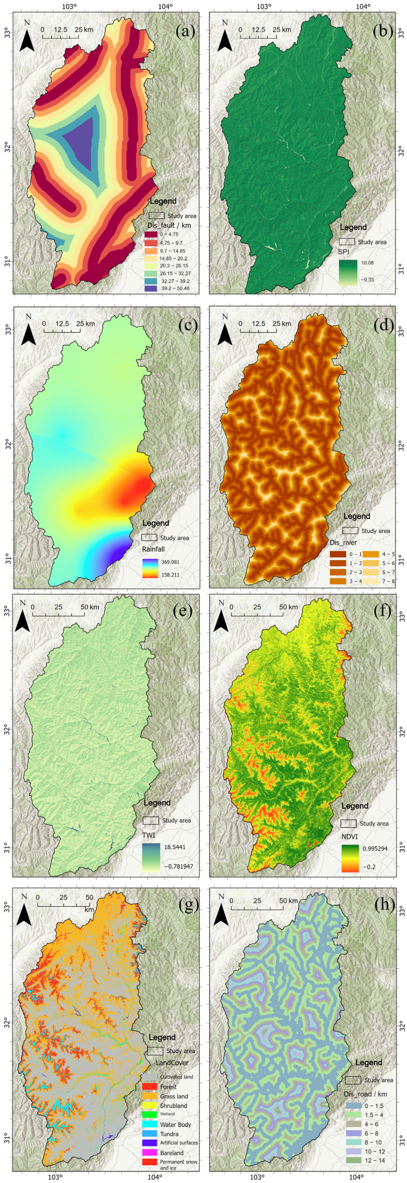
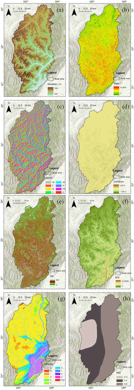
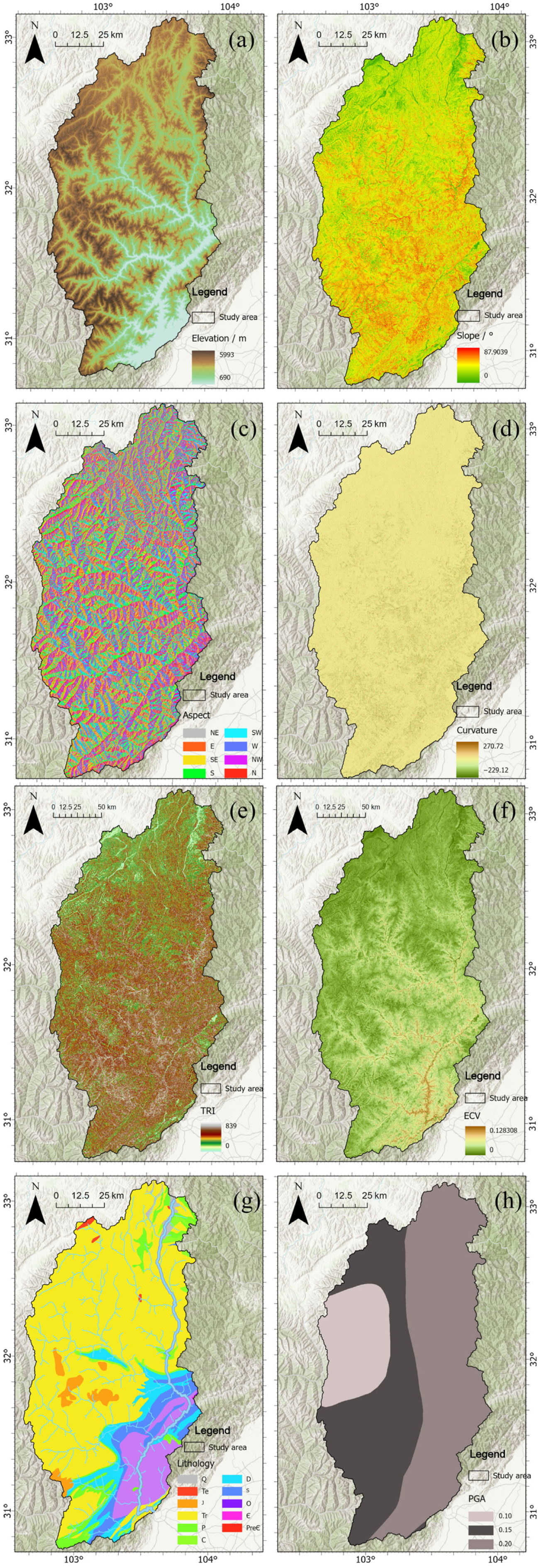
Figure 2 shows the distribution of the first eight disaster-inducing factors; the distribution of the remaining eight factors is presented in Appendix A. By considering these influencing factors, this study aims to comprehensively reflect the complex interaction between variables and reveal their combined impact on the susceptibility of landslide geological disasters.

Figure 2. Landslide evaluation factor distribution map. (a) Elevation; (b) Slope; (c) Aspect; (d) Curvature; (e) TRI; (f) ECV; (g) Lithology; (h) PGA.

2.3. Methods

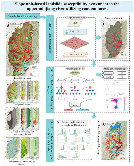
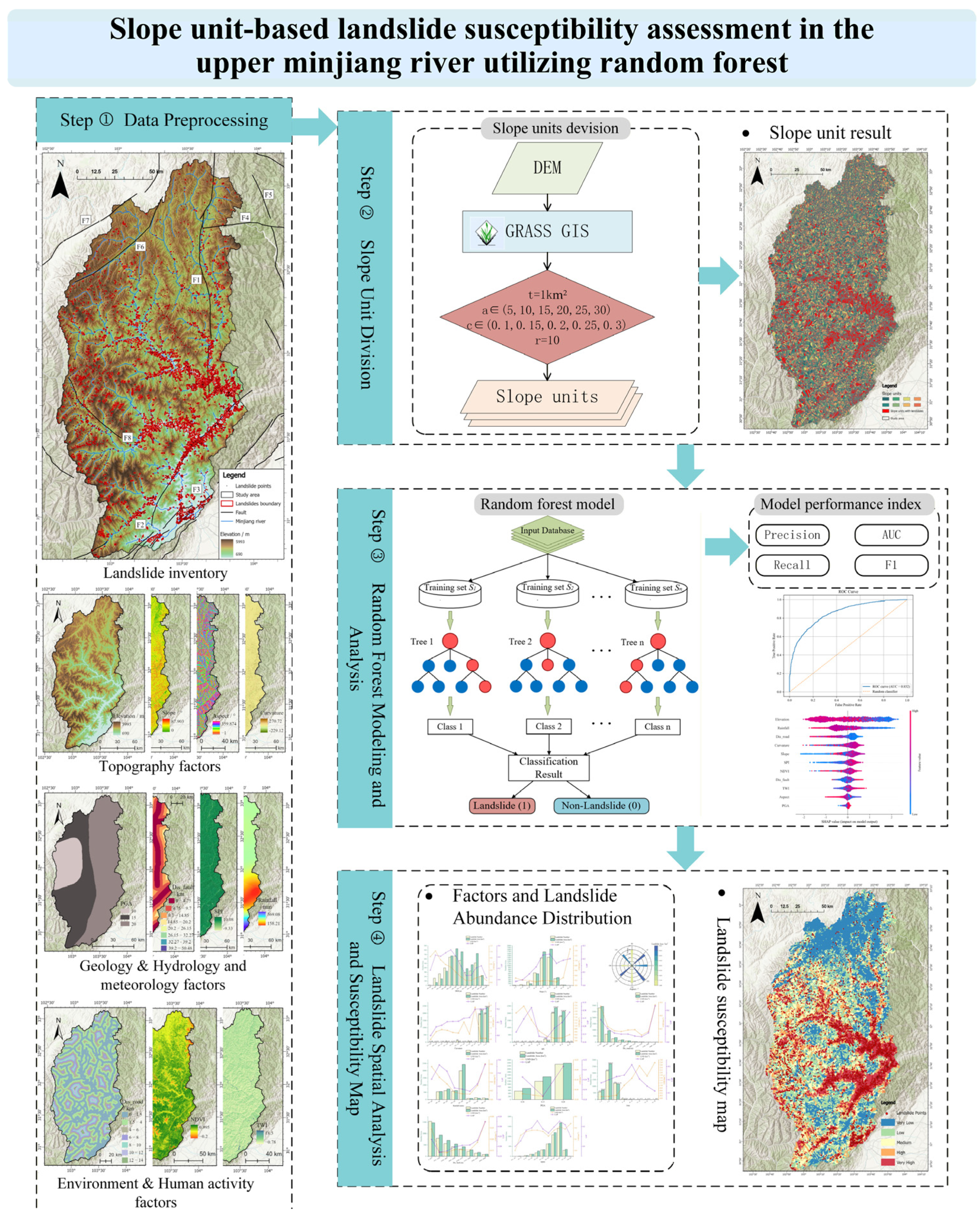
This paper develops a predictive framework for assessing regional landslide susceptibility using a machine learning model at the slope unit scale. The specific research steps include (see Figure 3):

Figure 3. The framework of the study.

• Establishing a landslide inventory: Based on multi-source satellite imagery, an interactive landslide relic interpretation method is used to establish a landslide relic database for the upper Minjiang River;
• Slope unit division: Utilizing the r.slopeunits tool to generate multiple slope unit layers under different parametric constraints;
• Ideal combination selection: The ideal parameter combination for slope unit division is selected based on the normalized superposition method of slope aspect standard deviation and global Moran’s I;
• Environmental factor extraction: Environmental factors such as topography, geology, meteorology, hydrology, and human engineering activities in the study area are extracted based on slope units to analyze the spatial characteristics of landslide development. Continuous factors were characterized by the average value of the raster values within the unit, while discrete factors were represented by the mode of the raster values for the corresponding slope unit;
• Landslide susceptibility modeling: Integrating optimized slope units with the Random Forest algorithm, this study constructs a robust landslide susceptibility assessment model to capture complex nonlinear geo-environmental relationships;
• Model accuracy evaluation: ROC curves and F1 are used to analyze the model accuracy;
• Producing a comprehensive regional map to visualize landslide susceptibility patterns.

2.3.1. Landslide Identification and Classification

Existing landslide trace interpretation techniques primarily include field surveys [39], automated recognition technologies [40], and human–machine interactive interpretation methods utilizing satellite imagery [41,42,43]. The Google Earth platform provides access to multi-temporal, sub-meter resolution optical satellite imagery. We employed a human–computer interactive method for interpreting landslide remnants [44,45], establishing identification criteria based on landslide formation conditions and topographic features [46]. These criteria facilitate the precise delineation of the spatial coordinates, aerial extent, and morphological configuration of individual landslide events [47,48]. This approach provides a thorough quantitative assessment of regional susceptibility while clarifying the spatial distribution patterns of landslide incidents within the upper Minjiang River [41,49]. The landslide identification criteria employed in this study primarily include: slope morphology resembling a reclining chair with tensile fissures at the rear edge; the middle and rear portions of the landslide body formed platform-like depressions, with cracks scattered along the front and middle margins; irregular terraces developed on the landslide body [50]; and clearly defined landslide boundaries or fissures developed along the slope body boundary [32].

The spatial heterogeneity and developmental traits of geohazards are predominantly expressed through distribution mapping, kernel density estimation, or descriptive frameworks [51,52]. Regional risk potential is typically evaluated through susceptibility zonation, which uses a categorical ranking from high to negligible susceptibility. Furthermore, geohazard density—defined as the concentration of occurrences per spatial unit—is further distinguished into point-based and area-based metrics. In this study, we used the GeoScene 2.1 platform and selected a search radius of 5 km to calculate the landslide number density (LND) and landslide area percentage (LAP) to analyze the relationship between landslide occurrence and influencing factors. The spatial intensity of landslide occurrences was quantified using the Kernel Density method, specifically adopting a fourth-order kernel function [53] to delineate regional hotspots. The density values are derived according to the following equation:

$$Density={\displaystyle \frac{1}{{\left(radius\right)}^2}}\sum _{i=1}^n\left[{\displaystyle \frac{3}{\pi }}·{pop}_i{\left(1-{\left({\displaystyle \frac{{dist}_i}{radius}}\right)}^2\right)}^2\right],For dis{t}_i<radius$$

(1)

where $i$ = 1, …, $n$ are the input points. Only include points in the sum if they are within the radius distance of the (x, y) location. ${pop}_i$ is the population field value of point $i$. ${dist}_i$ is the distance between point $i$ and the (x, y) location [54].

To maintain consistency with prevailing classification standards, the magnitude of landslide events is categorized based on volumetric estimates. These values are derived from validated power law empirical equations that correlate landslide surface area with its corresponding volume [55] (Formula (2)), thereby enabling quantitative characterization of landslide scale. In the absence of fine spatial scale information, this empirical formula does not need to specify the scale, spatial location, failure process, and its triggering mechanism of the landslide, so it is widely used to estimate the landslide volume based on the landslide area [56]:

$$V_L=\alpha {A_L}^{\beta }$$

(2)

where $\alpha$ and $\beta$ are empirical unknown constants to be regressed. To standardize the evaluation of landslide scales, this research adopted the volumetric taxonomy established by McColl and Cook [57]. Landslides were systematically grouped into six classes based on their estimated volumes ($V$): very small (10⁻³–10⁰ m³), small (10–10³ m³), medium (10³–10⁶ m³), large (10⁶–10⁹ m³), giant (10⁹–10¹² m³), and monster (10¹²–10¹⁵ m³). At the same time, combined with the landslide movement stage naming method proposed by Cruden and Varnes [58], this study developed a comprehensive classification and identification process, thereby ensuring a comprehensive characterization of landslide types and evolution characteristics in the study area.

2.3.2. The r.slopeunits Tool

Mapping units are the smallest indivisible spatial entities for geological hazard assessment and are a key foundation for regional landslide susceptibility assessments [21,59]. This study implements the r.slopeunits algorithm within the GRASS GIS computational environment to facilitate the automated delineation of slope units across the study area [23,60]. This method uses topographic slope aspect as the dividing standard, and the required parameters are shown in Table 2. The two key geomorphic factors that determine the unique scale and orientation of slope unit subdivisions are the minimum runoff area ($a$) and the minimum circular variance ($c$). The parameter $\left(a\right)$ determines the minimum contributing area required to initiate channelized flow and therefore controls the overall size of slope units. Larger values generally lead to coarser terrain segmentation and fewer slope units. The parameter $\left(c\right)$ represents the allowed variability of slope aspect within each unit and therefore regulates the internal directional consistency of slope units. Smaller values enforce stricter aspect homogeneity, producing more fragmented units. The spatial representation of landform features is directly impacted by these parameters. In addition, the primary role of parameters such as the iteration coefficient ($r$) and the initial flow accumulation threshold ($t$) is to ensure numerical convergence during the calculation process [19]. Additional parameters such as the iteration coefficient $\left(r\right)$ and the initial flow accumulation threshold ($t$) mainly control the convergence behavior of the algorithm during the iterative segmentation process and do not directly represent geomorphological properties.

Table 2. Parameters of r.slopeunits.

Parameters	Parameter Meaning	Value Range
t (m2)	Initial threshold (m2), threshold of the flow area.	1,000,000
r	Factor used to iteratively reduce initial threshold, iterative coefficient	10
a (×104 m2)	Minimum area (m2) below which the slope unit is not further segmented.	5, 10, 15, 20, 25, 30
c	Minimum value of the circular variance (0.0–1.0) below which the slope unit is not further segmented.	0.10, 0.15, 0.20, 0.25, 0.30

To evaluate the efficacy of various parameter configurations, this study implemented a normalized overlay analysis integrating aspect standard deviation and Global Moran’s I. This approach facilitates a rigorous assessment of intra-unit homogeneity and inter-unit heterogeneity, enabling the identification of the optimal slope unit configuration that best represents the underlying terrain. In particular, the slope unit’s internal homogeneity is larger when the aspect standard deviation is smaller, while its external heterogeneity is stronger when the global Moran’s index is smaller.

Using the raster-based slope units generated by r.slopeunits as the primary input, this study utilized the ArcGIS 10.8 platform to perform raster-to-vector conversion. This transformation ensures seamless data interoperability for subsequent spatial topological analysis, cartographic visualization, the spatial joins with landslide inventory data. Landslide units are identified based on a landslide area exceeding 2% of the slope unit area [61,62], and their influencing factor characteristics are extracted using a zonal statistical method. Continuous factors are represented by the average raster values within the unit, while discrete factors are represented by the mode of the raster values for the corresponding slope unit.

2.3.3. Random Forest Model

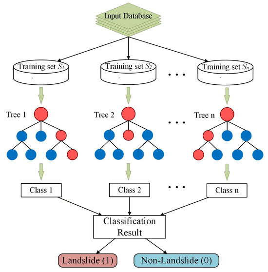
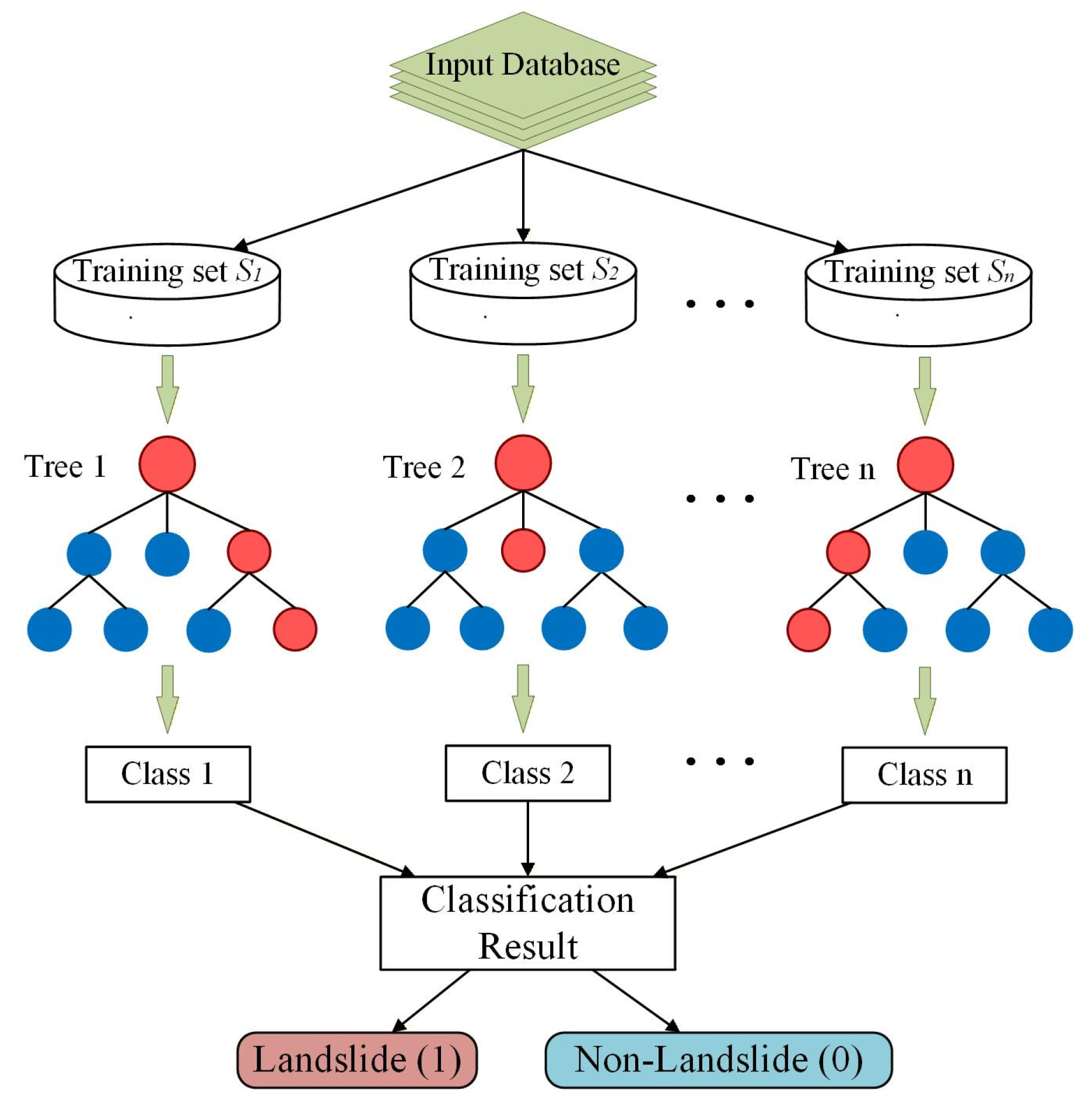
Random Forest (RF), originally conceptualized by Breiman, is a robust non-parametric supervised learning paradigm [16] that belongs to the ensemble learning paradigm. The algorithm employs bootstrap aggregating (bagging) to generate an ensemble of decorrelated decision trees, with a plurality voting mechanism used to synthesize the final classification output (Figure 4). By aggregating diverse base learners, this ensemble framework effectively attenuates the high variance associated with individual trees, thereby mitigating the risk of overfitting. The robustness and generalization performance of the model are significantly improved. RF has no prior assumptions about the distributional characteristics of the input variables and is well-suited to handling high-dimensional features. The model can capture complex nonlinear responses and is widely used in (LSM) [59,63,64].

Figure 4. Random forest model flowchart.

During model construction, RF introduces random feature subsets at the node splitting stage. This mechanism effectively weakens collinearity among evaluation factors, enabling it to robustly characterize the landslide occurrence mechanism driven by topography, geology, and triggering factors. Previous studies have shown that Random Forest (RF) often achieves strong or competitive predictive performance in landslide susceptibility assessment [65,66]. In this study, the slope unit is used serves as the smallest mapping unit. By using equal numbers of non-landslide and landslide sample sets, the model was carefully trained to unravel the complex nonlinear relationship between historical landslide spatial patterns and associated geo-environmental factors. The model was then extended across the entire study area to estimate and project landslide susceptibility probability at a regional scale using this learned relationship.

Each slope unit represents a single sample in the modeling dataset, where the dependent variable indicates the presence or absence of landslides and the independent variables correspond to the extracted environmental factors. The dataset was randomly split into training and validation sets to evaluate the model’s predictive performance.

2.3.4. Model Accuracy Validation

To objectively evaluate the classification performance of the RF model for landslide prediction, this study uses an independent test set and assesses performance along two dimensions: prediction accuracy and physical interpretability. To assess the model’s global predictive performance, this study used a balanced dataset with an equal ratio (1:1) of landslide and non-landslide samples. The basic diagnostic criteria used were the Receiver Operating Characteristic (ROC) curve and its associated Area Under the Curve (AUC). A threshold-independent evaluation of the model’s discriminative capability is provided by the ROC curve, which successfully depicts the dynamic equilibrium between the True Positive Rate (TPR) and the False Positive Rate (FPR) across a continuous spectrum of probability thresholds. The resulting AUC value (0–1) provides an intuitive measure of model robustness, with higher values indicating stronger discrimination capability [67]. In addition, the F1-score, defined as the harmonic mean of precision and recall, was employed to further assess classification reliability and balance. Since conventional performance metrics do not explicitly reveal the internal decision-making mechanisms of machine-learning models, SHAP were subsequently applied to enhance model interpretability [68]. This method quantitatively assesses the marginal contribution of each conditioning factor to landslide probability, and clarifies the direction of their respective impacts.

3. Results and Analyses

3.1. Landslide Inventory

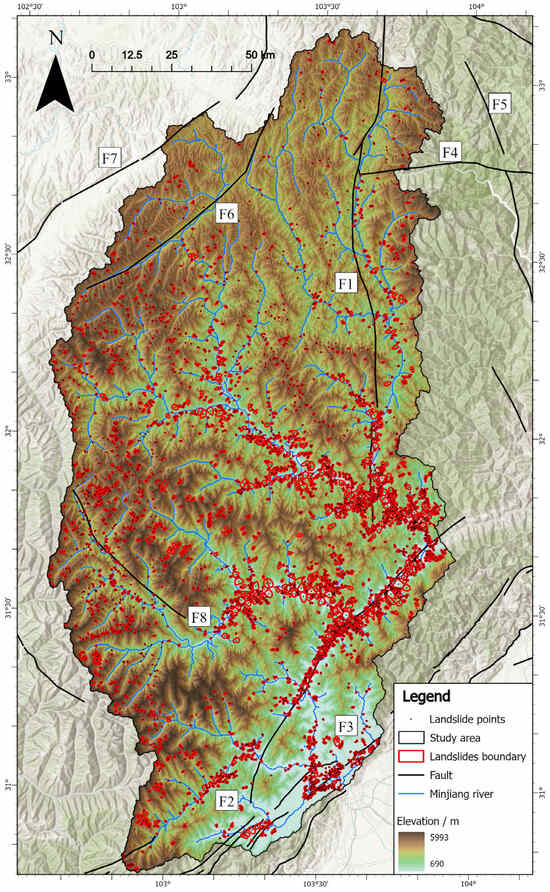
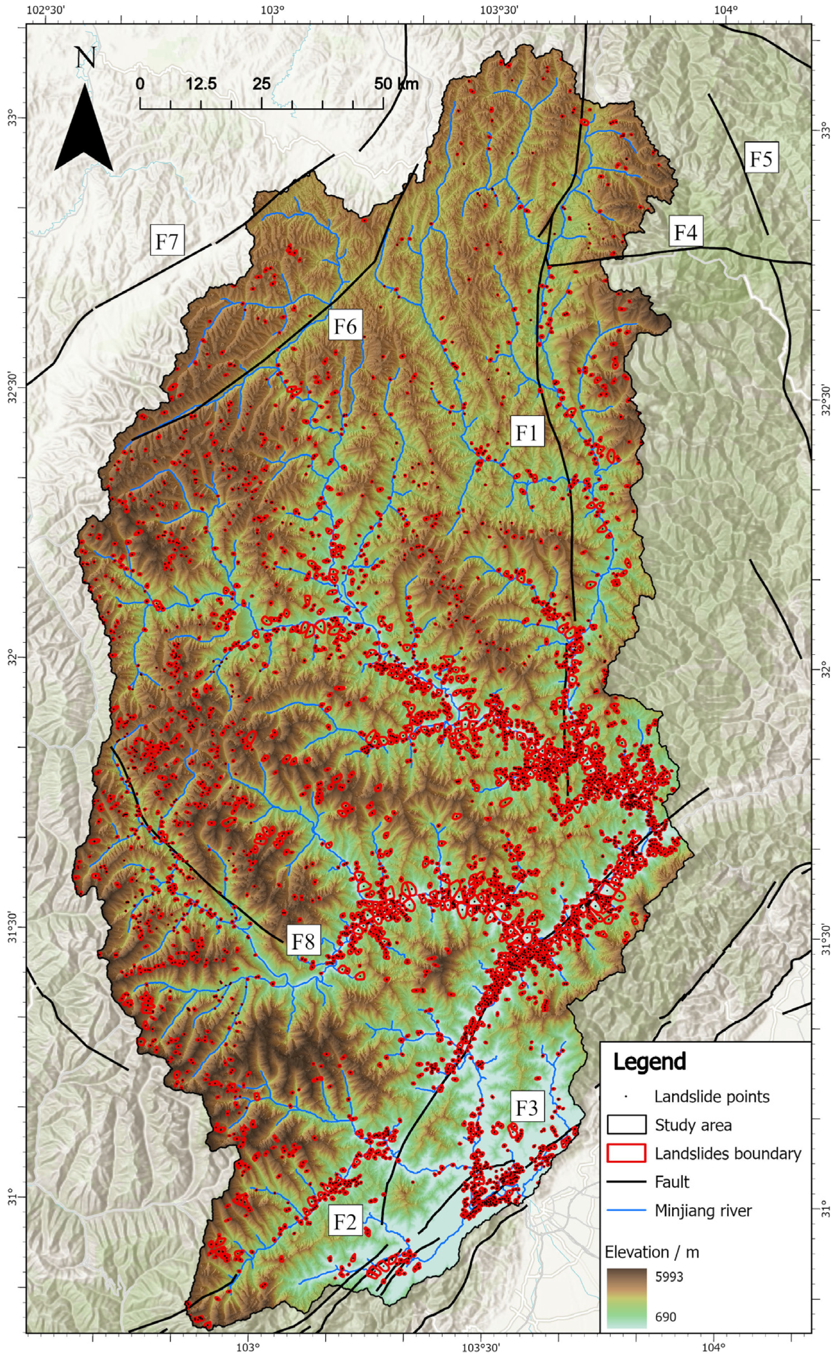
As illustrated in the landslide inventory map (Figure 5), the study area encompasses 3785 mapped landslides totaling 1271 km². The developmental intensity of these hazards was systematically evaluated through two key metrics: Landslide Number Density ($LND$) and Landslide Area Percentage ($LAP$), which were calculated using the following formulae:

$$LND=3785 \mathrm{p}\mathrm{i}\mathrm{e}\mathrm{c}\mathrm{e}/\mathrm{22,950}{\mathrm{k}\mathrm{m}}^2=0.165 {\mathrm{p}\mathrm{i}\mathrm{e}\mathrm{c}\mathrm{e}/\mathrm{k}\mathrm{m}}^2$$

$$LAP=1271 {\mathrm{k}\mathrm{m}}^2/\mathrm{22,950}{\mathrm{k}\mathrm{m}}^2\times 100\%=5.54\%$$

Figure 5. Landslide relics distribution map. In the figure, F1 is the Mijiang Fault; F2 is the Wenchuan–Maowen Fault; F3 is the Beichuan–Yingxiu Fault; F4 is the Xueshan Fault; F5 is the Huya Fault; F6 is the Maoergai Fault; F7 is the Longriba Fault; F8 is the Miyaluo Fault.

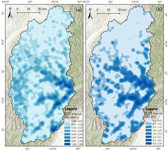
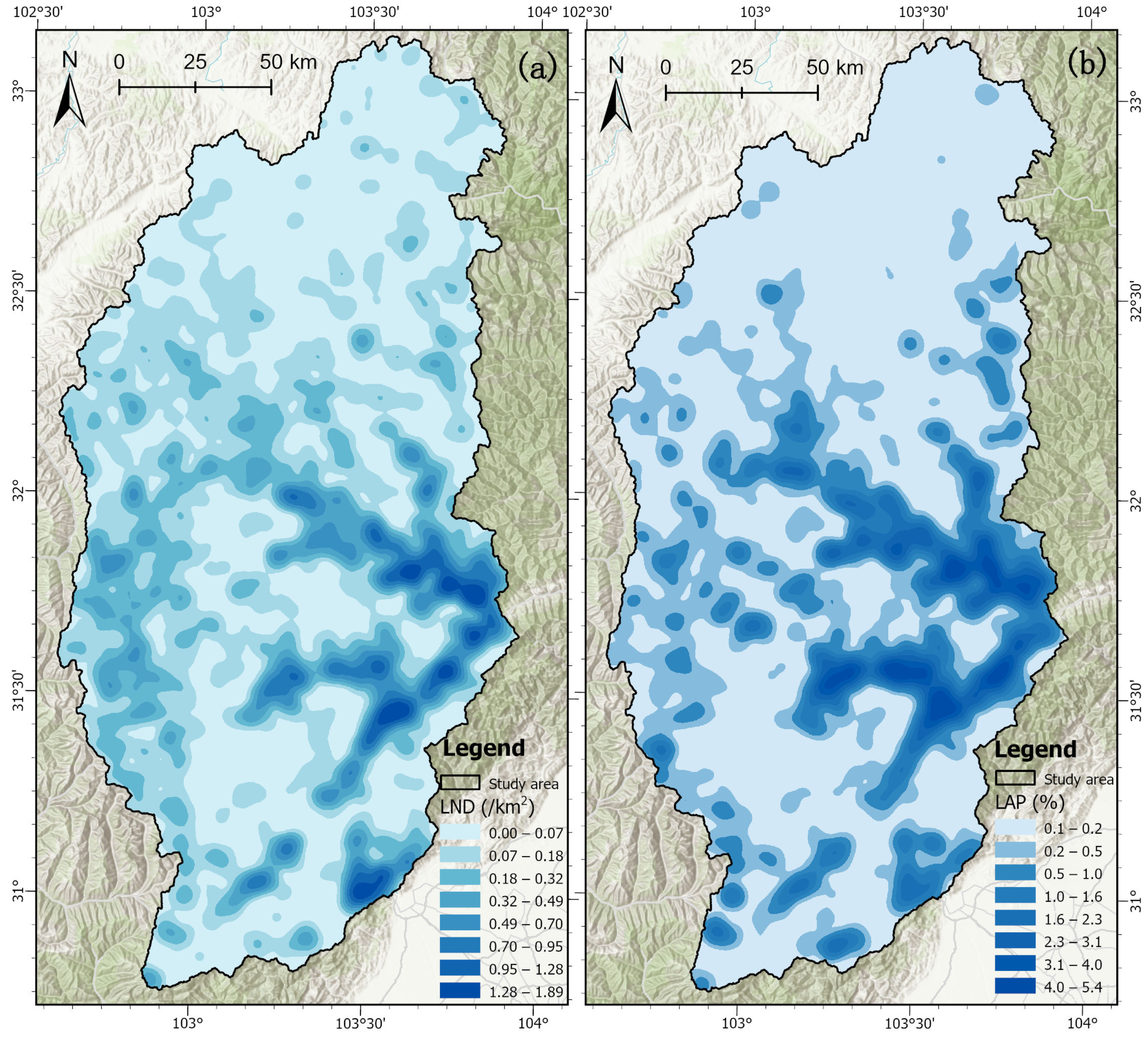
Figure 6a and Figure 6b, respectively, display LND and LAP computed using ArcGIS. The calculation results show that the LND ranges from 0 to 1.89 pieces/km² in the study area. The area with an LND less than 0.7 km⁻² is approximately 22,020 km², accounting for 95.95% of the full study area; the area with an LND greater than 0.7 pieces/km² and less than 1.89 pieces/km² is approximately 930 km², accounting for 4.05% of the total area. The LAP ranges from 0 to 5.4% in the study area. The largest proportion (87.77%) has an LAP of less than 1%, covering an area of approximately 20,143 km². The area with an LAP greater than 1% and less than 4% is approximately 2620 km², representing for 11.41% of the total area; the region with an LAP greater than 4% is approximately 1.02%, covering an area of approximately 187 km². Both metrics reflect landslide intensity but capture different aspects: LND emphasizes the frequency of landslide events, whereas LAP reflects the spatial extent of landsliding. In our analysis, LND and LAP show broadly similar spatial trends, but LAP tends to highlight regions with larger landslides more prominently.

Figure 6. Map of landslide density. (a) LND; (b) LAP.

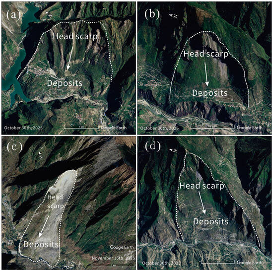
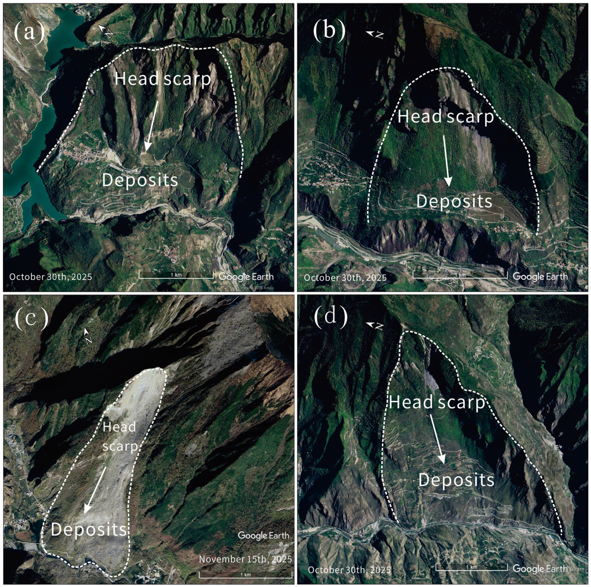
As evidenced by the inventory and density distribution maps, landslide development in the upper Minjiang River exhibits distinct spatial clustering. Significant spatial clustering within high-relief alpine canyons and along the main river channels, especially the Zagunao and Heishui basins, is a characteristic of landslides in the upper Minjiang River, and dense distribution along some fault zones, such as the Wenchuan–Maowen Fault, the Beichuan–Yingxiu Fault, and the Minjiang Fault. This study selected four typical landslides for display (see Figure 7), namely the Diexi landslide [69], Manaoding landslide [70], Xinmo landslide [71,72], and Yejiping landslide [70,73]. The typical landslides in these landslide lists are highly consistent with previous studies in terms of geographical location, morphological characteristics, and extent of deposits.

Figure 7. Typical landslide relics display map. (a) Diexi Landslide is located at 32.04° N, 103.69° E; (b) Mannaoding Landslide is located at 31.98° N, 103.68° E; (c) Xinmo Landslide is located at 32.07° N, 103.66° E; (d) Yejiping Landslide is located at 31.88° N, 103.70° E. These landslides all occurred on the left bank of the Minjing River’s flow direction.

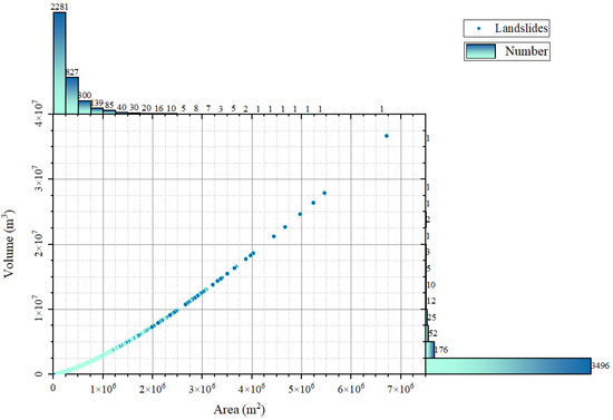
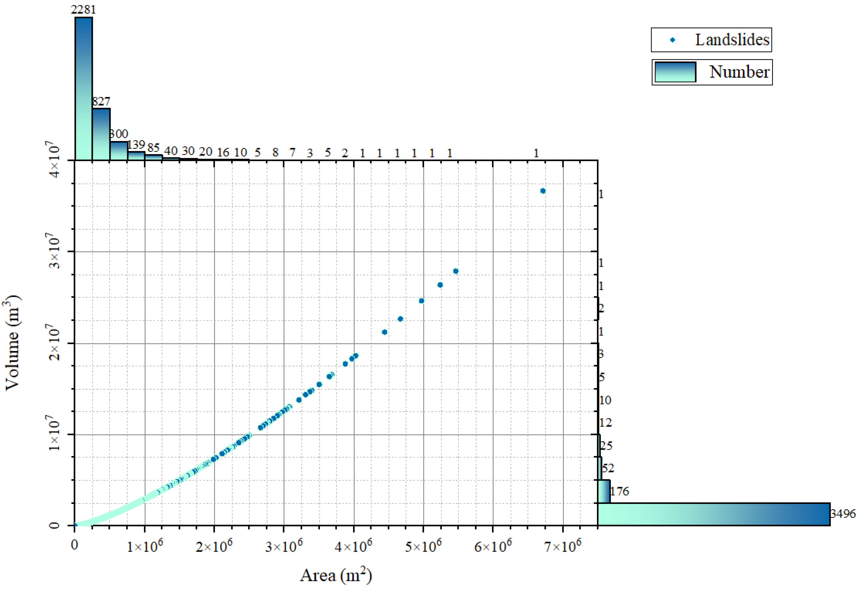
This study uses the landslide volume estimation formula (Formula (2)), and the parameters α = 0.033 and β = 1.325 were adopted from Leong et al. [74], who reported them as average values compiled from published empirical area–volume relationships. In this study, these parameters were used only for relative magnitude classification and regional statistical analysis, rather than for precise volume estimation of individual landslides. Then, based on the six-level landslide scale description system proposed by McColl and Cook [57], the landslides in the upper Minjiang River are classified by scale. The landslide’s volume and area distribution are shown in Figure 8. According to the volume results, the research region has 787 large landslides, 2989 medium landslides, and 9 small landslides. The total landslide volume is about 3.36 × 10⁹ m³; the average is 8.88 × 10⁵ m³, the maximum is 3.67 × 10⁷ m³, and the median is 3.23 × 10⁵ m³.

Figure 8. Distribution of landslide area and volume scale.

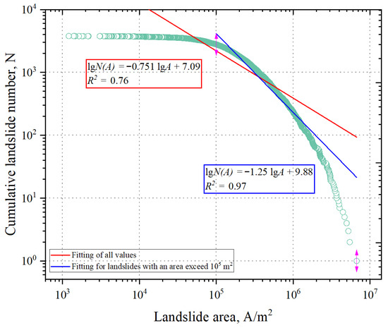
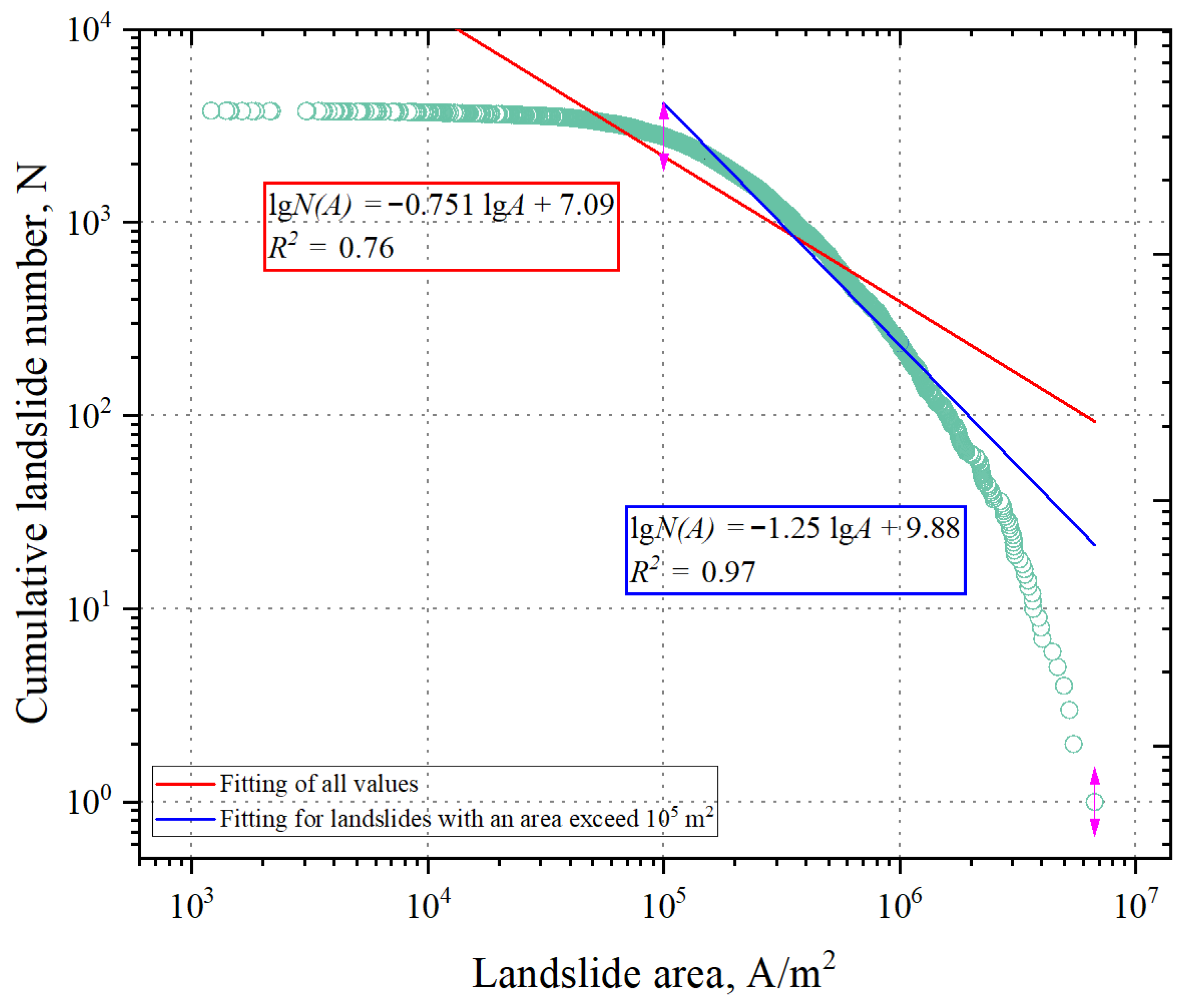
The amount of landslides and the landslide area typically follow a power law relationship [41] (Formula (3)). To show the scale characteristics of landslides in the upper Minjiang River, this study shows a double logarithmic plot of the total number of landslides versus landslide area.

$$lgN\left(A\right)=-\beta lg\left(A\right)+\alpha$$

(3)

where $N$ is the entry number of landslides that have exceeded area $A$, and $A$ is the landslide area [32]. The fitted curve for all landslides using a double logarithmic coordinate system is $lgN\left(A\right)=-0.751lg\left(A\right)+7.09, R^2=0.76$, as shown in Figure 9. The fitted curve for landslides with an area greater than 1 × 10⁵ m² is $lgN\left(A\right)=-1.25lg\left(A\right)+9.88, R^2=0.97$. In terms of scale distribution, the study area is dominated by small-scale landslide events, while the frequency of large-scale, high-intensity landslides remains statistically low. This frequency-scale pattern conforms to the actual power law distribution in the regional landslide catalog. The curve for areas less than 1 × 10⁴ m² is relatively flat, which may be because small landslides are difficult to identify in remote sensing images, resulting in some landslides not being counted.

Figure 9. Fitting curve for cumulative landslide number and landslide area.

In addition to the frequency–area analysis, the regional representativeness of the inventory is also supported by comparison with previous landslide studies in the upper Minjiang River [32], which generally reported substantially lower landslide number densities [75,76,77]. This suggests that the present inventory provides a denser and more detailed mapping of landslides at the regional scale.

3.2. Slop Units Division Results

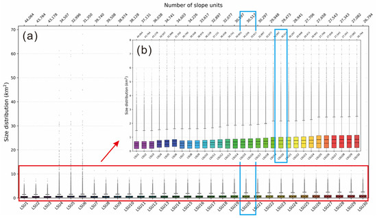
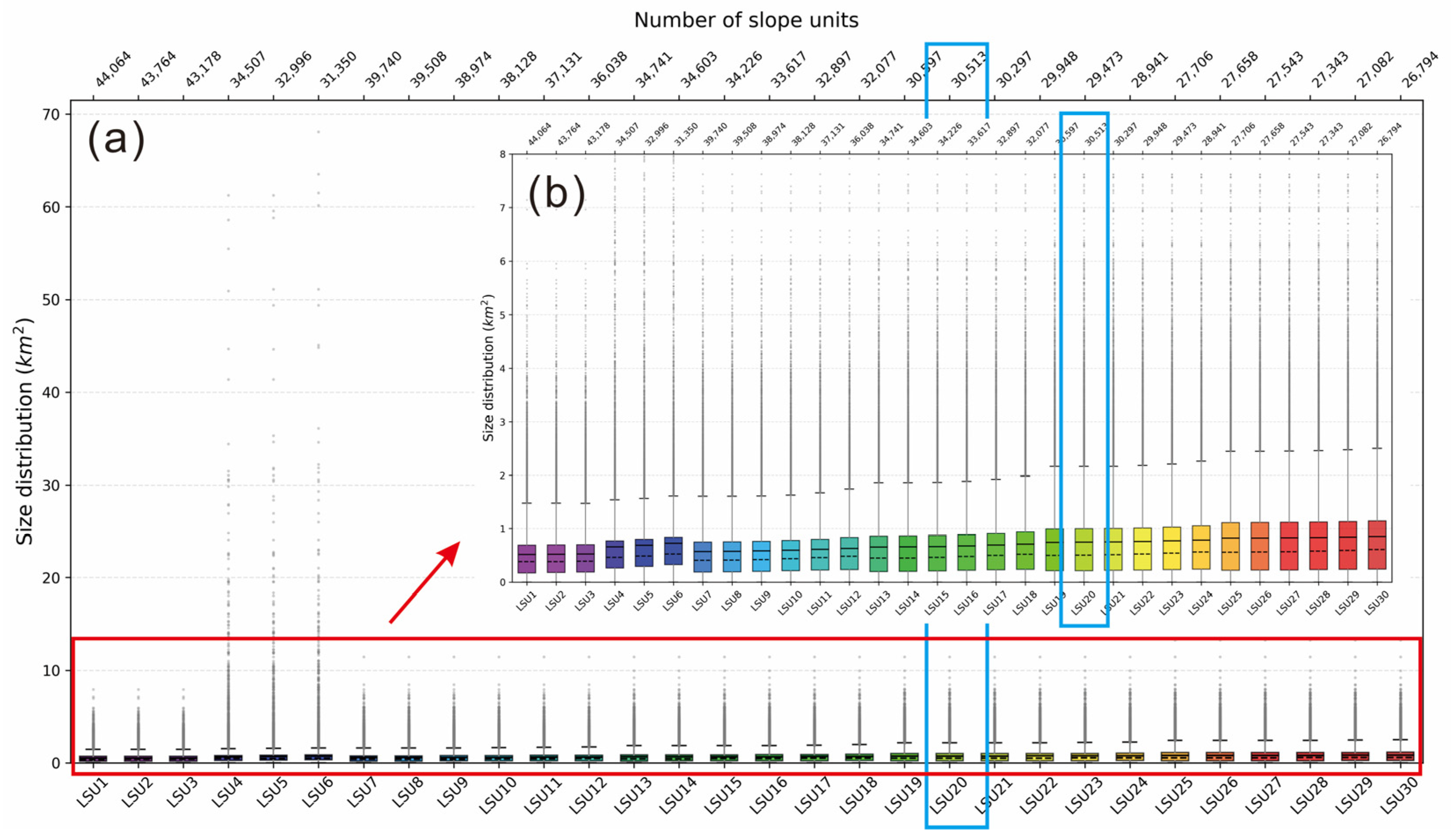
The r.slopunits method in GRASS GIS was used for the slope unit division in this investigation. Values for $a$ were selected as 5 × 10⁴ m², 1 × 10⁵ m², 1.5 × 10⁵ m², 2 × 10⁵ m², 2.5 × 10⁵ m², and 3 × 10⁵ m². Values for $c$ were selected as 0.1, 0.15, 0.2, 0.25, and 0.3, resulting in 30 different slope unit division methods, as shown in Table 3. The number and area distribution of the 30 slope unit divisions are seen in Figure 10. The mean distribution of slope unit area in (b) is represented by the solid black line in the box plot, whereas the median distribution is represented by the dashed black line.

Table 3. Slope units with different parameter combinations.

LSU_Number		The Minimum Area Threshold—a (×105 m2)
		0.5	1	1.5	2	2.5	3
The minimum circule variance within a slope—c	0.1	44,064(LSU1)	43,764(LSU2)	43,178(LSU3)	34,507(LSU4)	32,996(LSU5)	31,350(LSU6)
	0.15	39,740(LSU7)	39,508(LSU8)	38,974(LSU9)	38,128(LSU10)	37,131(LSU11)	36,038(LSU12)
	0.2	34,741(LSU13)	34,603(LSU14)	34,226(LSU15)	33,617(LSU16)	32,897(LSU17)	32,077(LSU18)
	0.25	30,597(LSU19)	30,513(LSU20)	30,297(LSU21)	29,948(LSU22)	29,473(LSU23)	28,941(LSU24)
	0.3	27,706(LSU25)	27,658(LSU26)	27,543(LSU27)	27,343(LSU28)	27,082(LSU29)	26,794(LSU30)

Figure 10. Box-plots show distribution of LSUs area. The bottom axis represents slope unit groupings, while the top axis indicates the number of slope units. The blue box indicates the ideal combination; (b) is an enlarged view of slope unit areas ranging from 0 to 8 km² in (a).

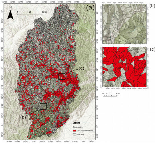
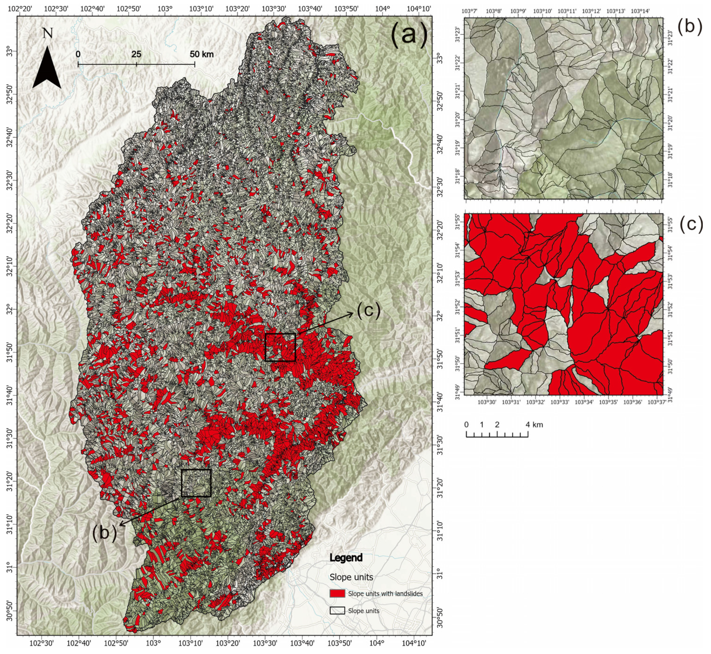
The ideal parameter combination obtained in this study was a = 1 × 10⁵ m², c = 0.25, dividing the study area into 30,513 slope units. The division results are shown in Figure 11a, with detailed diagrams in (b,c).

Figure 11. Slope unit results. (a) shows the division results for the entire study area. (b,c) present detailed views of the three boxes within (a). The red units indicate slope units containing landslides.

In landslide susceptibility assessment based on slope units, the proportion of landslide area within a slope unit to its total area is often used to determine whether a slope unit contains a landslide event [17,78]. This study, combining regional landslide scale and sample distribution characteristics, defines slope units where the landslide area exceeds 2% of the total slope unit area as landslide units, as shown in the red units in Figure 11a. To evaluate the sensitivity of this threshold, we tested it using 1%, 2%, 3%, and 5% as the criteria for defining landslide units. The results show that the number of landslide units extracted under the 1% and 2% thresholds were identical in this dataset. The RF model achieved the best performance at the 2% threshold (AUC = 0.852), while the AUC values decreased slightly to 0.845 and 0.844 under the 3% and 5% thresholds, respectively. These results suggest that the 2% threshold is a reasonable and robust choice for the present study. A total of 4057 slope units were selected as positive landslide unit samples; simultaneously, 4057 slope units that did not contain landslides were randomly selected as negative landslide unit samples.

3.3. Multicollinearity Analysis of Condition Factors

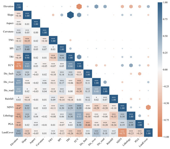
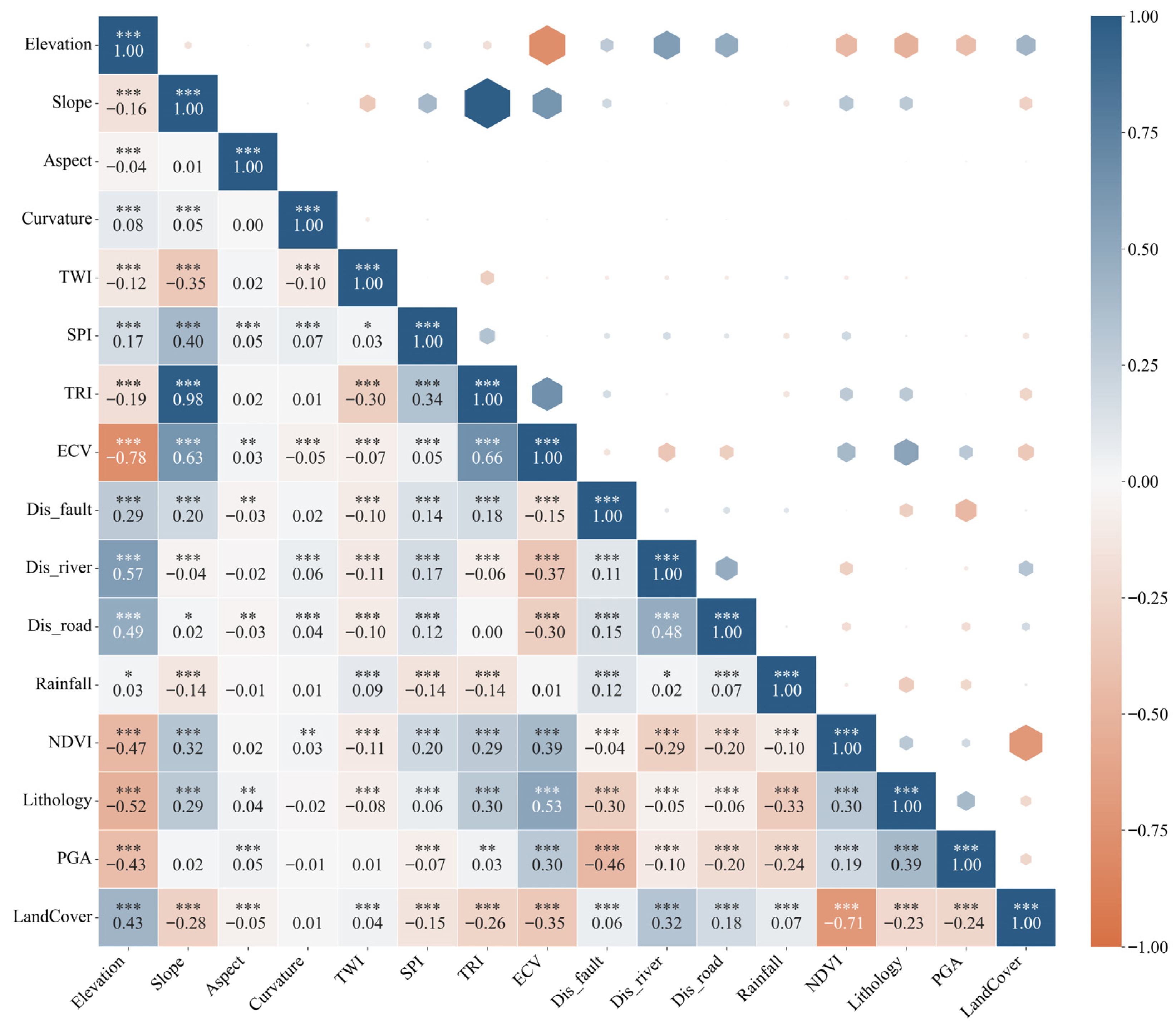
Although the RF model is relatively robust to multicollinearity, correlation analysis was performed to reduce redundancy among predictors and to obtain a more interpretable set of conditioning factors for subsequent modeling and SHAP analysis. Calculate the Pearson correlation coefficients of the influencing factors and plot a heatmap of the image factors. To ensure the independence of input variables, a threshold of 0.5 for the absolute Pearson correlation coefficient was established as the criterion for identifying collinearity. Any pair of quantitative factors exceeding this limit was considered to exhibit significant statistical redundancy, necessitating the exclusion of one variable from the assessment framework to prevent model bias. Figure 12 shows that TRI and Slope have correlation coefficients of 0.98, respectively; ECV and DEM and Slope have correlation coefficients of −0.78 and 0.63, respectively; Dis_river and DEM have a correlation coefficient of 0.57; Lithology and DEM and ECV have correlation coefficients of −0.52 and 0.53, respectively; and the correlation coefficient between Land Cover and NDVI is 0.71. All of these values are greater than the threshold of 0.5, indicating a strong correlation among these factors. Therefore, TRI, ECV, Dis_river, Lithology, and Land Cover are removed from the evaluation factors. After multicollinearity diagnosis, 5 redundant factors were excluded, and the remaining 11 factors were used for modeling.

Figure 12. Correlation Analysis Heatmap of evaluation factors. The size of the hexagon represents the absolute value of the correlation coefficient, and the color indicates the direction of the correlation. Asterisks indicate statistical significance: * p < 0.05, ** p < 0.01, *** p < 0.001.

3.4. GIS Spatial Characteristics Analysis of Landslide

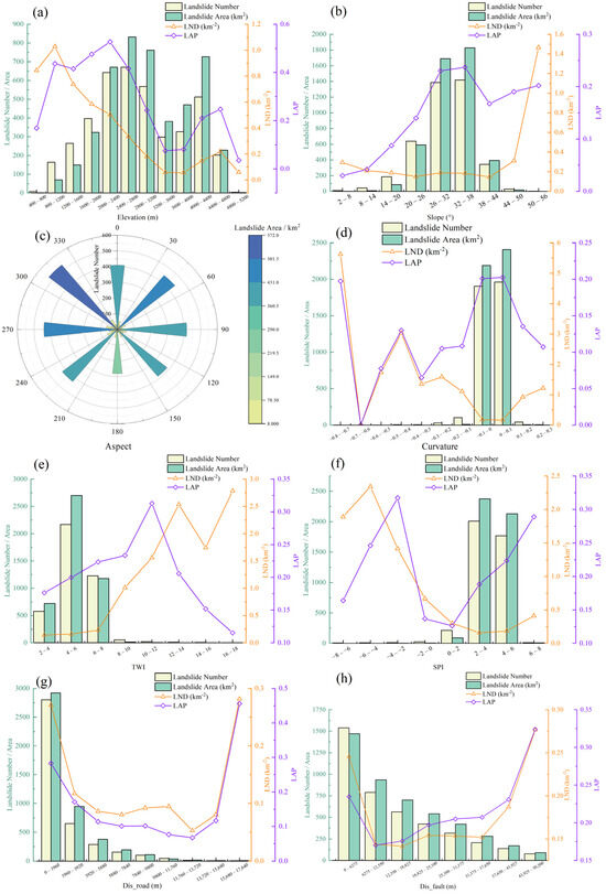
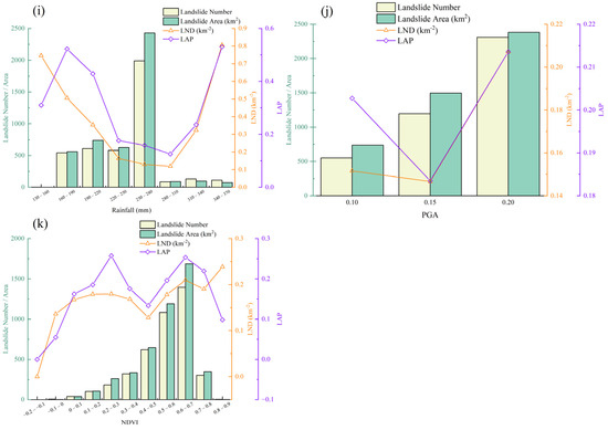
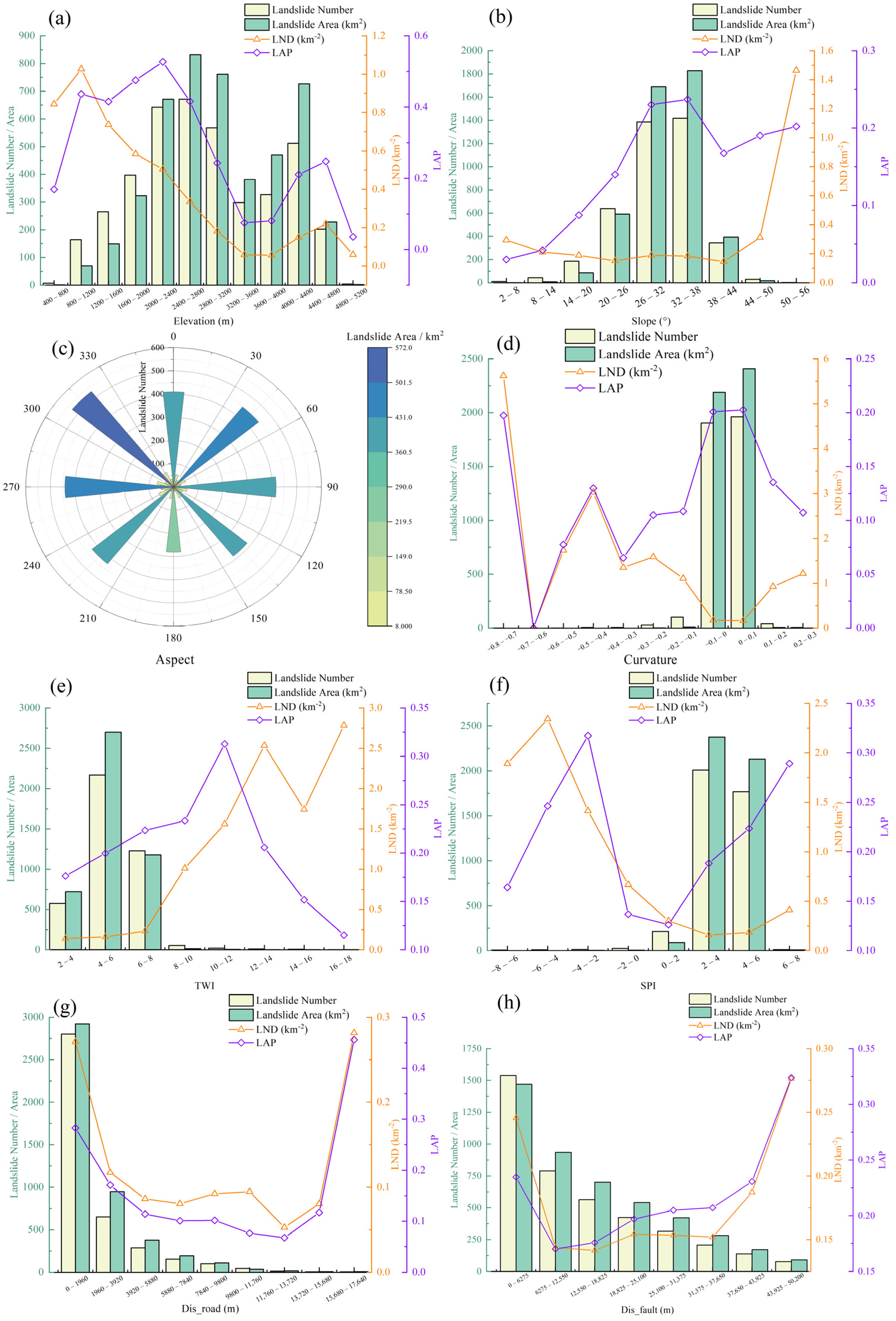
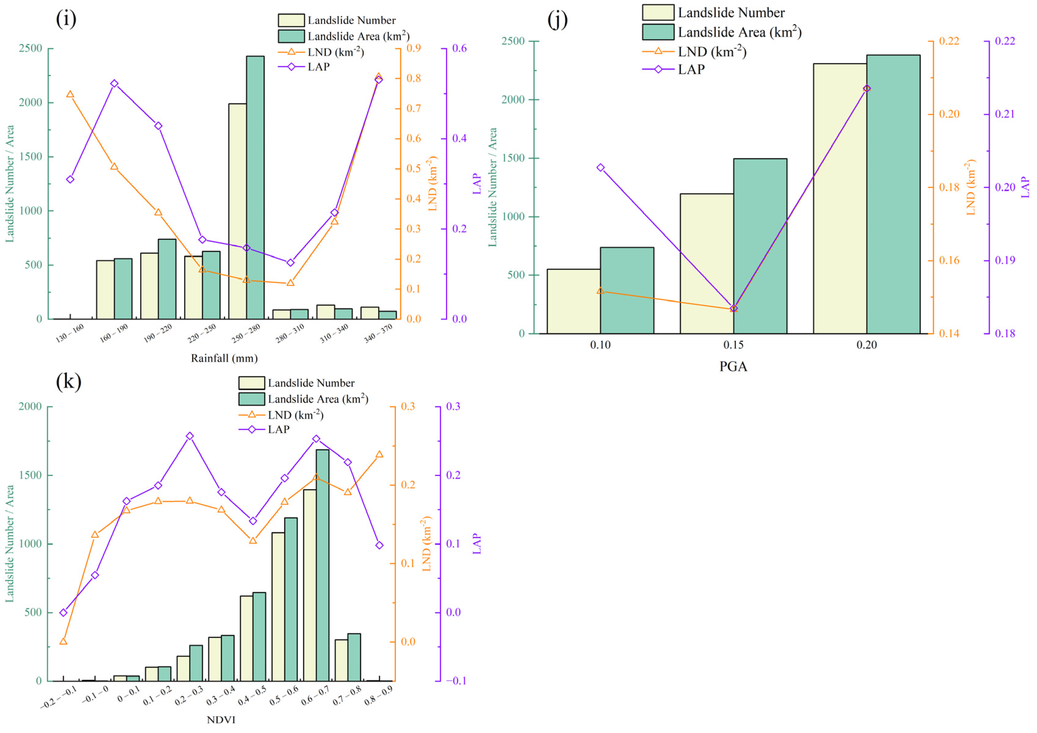
Ultimately, eleven geo-environmental conditioning factors were curated for the susceptibility modeling framework, encompassing diverse domains: topographic (Elevation, Slope, Aspect, Curvature, TWI, and SPI), geological and structural (Dis_fault and PGA), anthropogenic (Dis_road), vegetative (NDVI), and hydro-climatic (Rainfall). Figure 13 shows the correlation between the 11 selected evaluation factors and the number and area of landslides in the upper Minjiang River, as well as landslide abundance indices (LND and LAP), in order to illustrate the spatial correspondence between landslide distribution and the conditioning factors.

Figure 13. Correlation between evaluation factors and landslide density. (a) Elevation; (b) Slope; (c) Aspect; (d) Curvature; (e) TWI; (f) SPI; (g) Distance to road; (h) Distance to fault; (i) Rainfall; (j) PGA; (k) NDVI.

As shown in Figure 13, landslides in the upper Minjiang River reach their maximum number and area at high altitudes (2400–2800 m) and steep slopes (32–38°), as shown in Figure 13a,b. The distribution of landslides varies significantly with slope direction, with a greater concentration in the northwest. Concave areas (curvature −0.5 to −0.4) exhibit relatively high landslide density, as shown in Figure 13d. With increasing TWI, the number and density of landslides initially increase and then decrease, reaching their maximum at topographic wetness levels of 4–6, as shown in Figure 13e. Strong stream intensity favors landslide development, as seen in the SPI. The number and area of landslides were highest between 2 and 4, as shown in Figure 13f. The distribution of landslides showed a significant negative correlation with the distance from roads and faults, with landslides being more densely distributed closer to roads and faults, as shown in Figure 13g,h. Landslides were concentrated under moderate rainfall conditions of 250–280 mm, as shown in Figure 13i. The results in Figure 13j show that landslides in the upper Minjiang River are concentrated in areas with high peak ground acceleration, suggesting that strong earthquakes are closely associated with landslide occurrence in the study area. Landslides are relatively concentrated in regions with high vegetation cover and an NDVI of 0.6–0.7, as seen in Figure 13k, although this pattern may partly reflect the elevation band in which both higher NDVI values and dense landslide occurrence co-occur.

3.5. Landslide Susceptibility Mapping Analysis

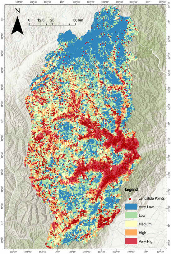
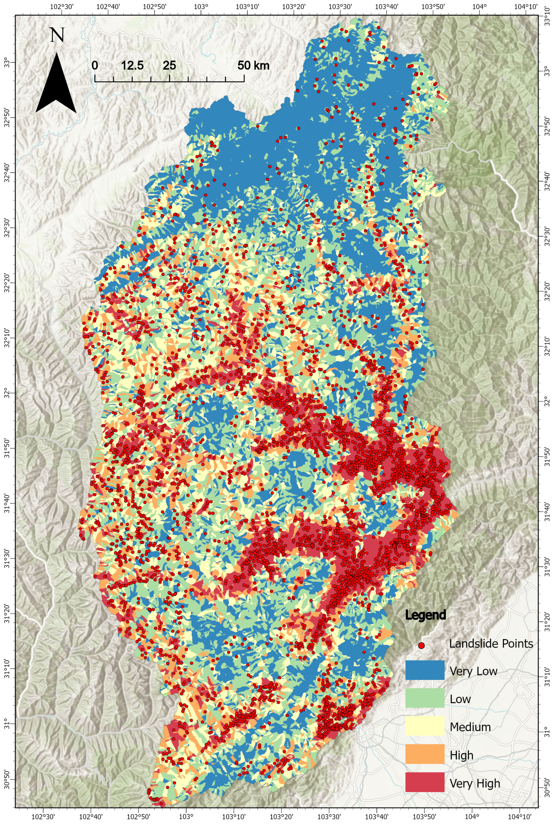
A stratified random sample technique was used to divide the data into training and validation subsets while preserving a 70/30 split ratio using the built landslide susceptibility framework This approach ensured that the prevalence of landslide and non-landslide samples remained consistent across both subsets, thereby preserving the statistical integrity of the model. Subsequent evaluation using the independent test set confirmed the model’s robust discriminative capacity and predictive stability in differentiating between landslide and non-landslide slope units. Figure 14 shows the regional distribution characteristics of the resultant susceptibility levels. Specifically, zones characterized by very low landslide susceptibility account for approximately 28% of the entire study region and are mainly clustered around Chuanzhusi Town and Maoergai Town in the northern sector. Areas classified as low susceptibility are spatially scattered and represent nearly one quarter (about 25%) of the study area, whereas regions with moderate susceptibility occupy roughly 17%. High-susceptibility zones cover around 14% of the area, while very high susceptibility zones constitute approximately 16%. Beyond their partial alignment with major fault systems—most notably the Wenchuan–Maowen, Minjiang, and Beichuan–Yingxiu fault zones—areas with high and very high landslide susceptibility are predominantly distributed along principal river corridors, especially within the Zagunao and Heishui river basins, reflecting the strong influence of fluvial erosion processes.

Figure 14. Landslide susceptibility map. Red dots indicate landslide points.

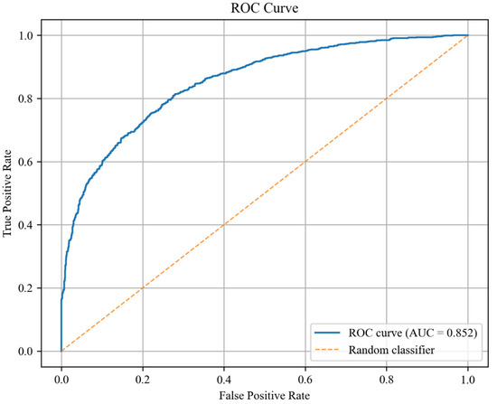
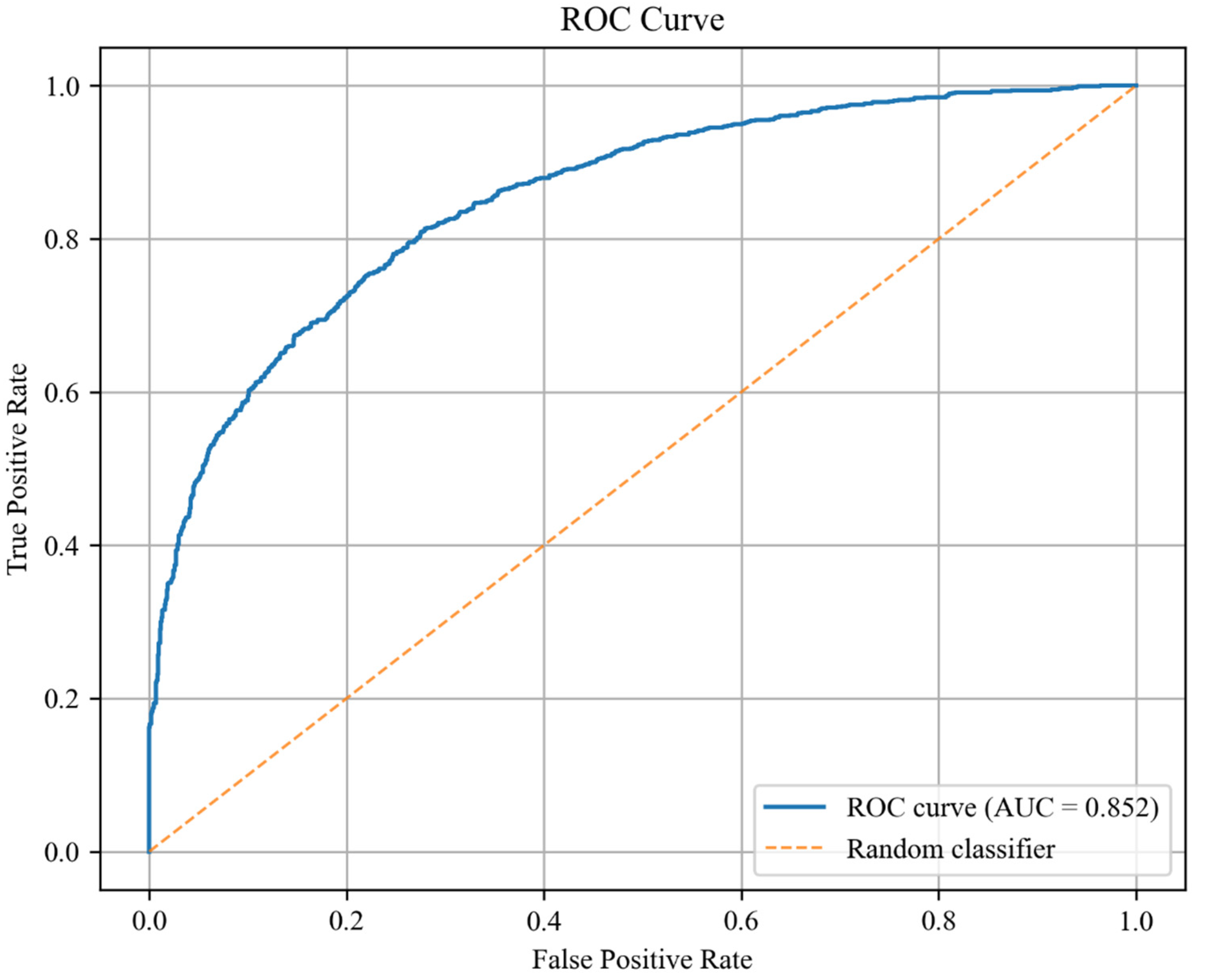
ROC curve analysis yielded an AUC value of 0.852 (as shown in Figure 15), indicating that the model performs well in balancing overall prediction accuracy and landslide unit identification ability. Table 4 shows that the model’s overall prediction accuracy is 0.77 at a threshold of 0.5, with precision and recall of 0.78 and 0.75, respectively, indicating relatively balanced identification performance.

Figure 15. The ROC curve of the random forest model in the assessment landslide susceptibility.

Table 4. Classification performance of the Random Forest model for slope-unit-based landslide susceptibility mapping, including precision, recall, F1-score, and support for landslide (1) and non-landslide (0) classes.

	Precision	Recall	F1-Score	Support
0	0.76	0.78	0.77	1218
1	0.78	0.75	0.76	1217

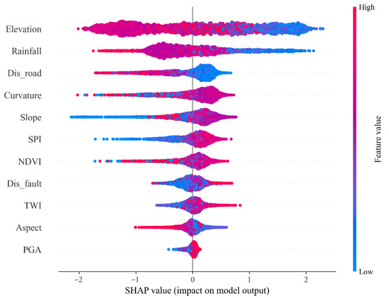
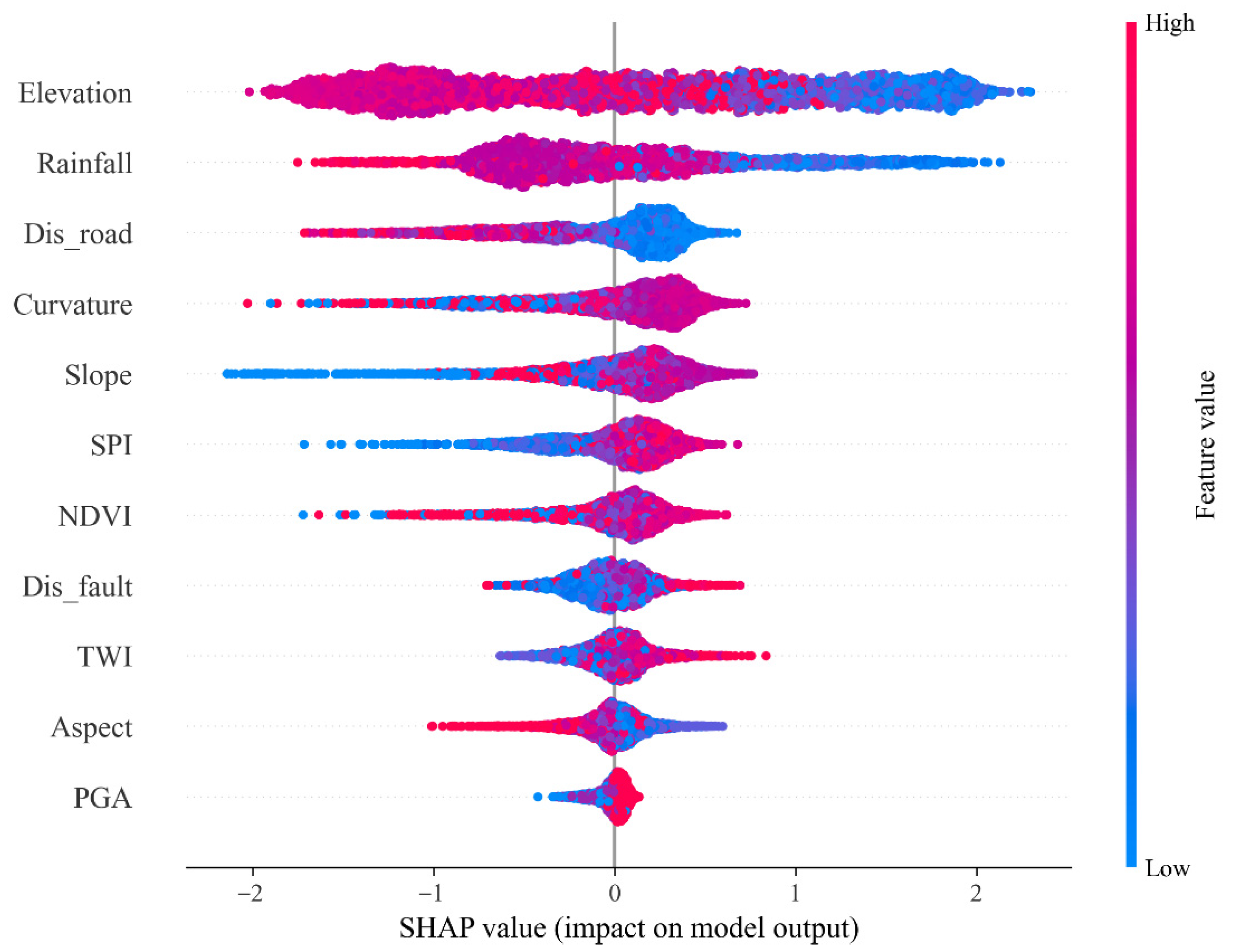
Building upon this, the SHAP method was used to further reveal the driving mechanism underlying the model’s results through interpretability analysis. The SHAP summary plot (Figure 16) shows that different environmental factors contribute significantly to landslide susceptibility, and their effects exhibit obvious nonlinear characteristics. Overall, topographic and meteorological factors dominate the model.

Figure 16. SHAP summary plot. The SHAP values are displayed on the horizontal axis; positive values indicate an increased probability of landslides, while negative values indicate a decreased probability. The color gradient represents the feature values, with red indicating high values and blue indicating low values.

Among them, elevation and rainfall have the most significant impact on the model output. The effect of elevation is somewhat complex: lower elevations (shown in blue in the feature map) are generally associated with an increased likelihood of landslides, while higher elevations (shown in red in the feature map) are associated with a decreased probability of landslides. Rainfall also plays a significant role; high levels of rainfall may increase the likelihood of landslides. The SHAP distribution of distance to road shows that slope units closer to the road have a significant positive contribution to landslide susceptibility, reflecting the weakening effect of engineering disturbances on slope stability. Slope and curvature also have significant effects on landslide occurrence; larger slopes and unfavorable topographic features enhance gravity-driven effects and stress concentration conditions. Additionally, hydrological variables, such as the SPI and TWI, showed significant positive effects in specific regions, suggesting that groundwater conditions and surface runoff convergence are crucial for the start and progression of landslides.

Overall, the SHAP-based interpretation not only confirmed the soundness of the model’s predictive outcomes but also elucidated, in a data-oriented manner, the coupled influence of multiple controlling factors on landslide susceptibility across the study region, thereby offering a robust foundation for further analyses of susceptibility zoning and landslide formation mechanisms.

4. Discussions

4.1. The Impact of Key Factors on Landslides

This study employs the SHAP tool to provide a global interpretation of the RF model. This interpretation is based on the average of the absolute SHAP values for each feature, which measures the average marginal contribution of the feature to the model’s prediction of the target [68]. Unlike traditional measures of feature importance, the average SHAP value not only reflects the typical influence of a feature on landslide susceptibility predictions across the entire dataset but also identifies key environmental factors that trigger landslides more rigorously by accounting for interactions among features [19].

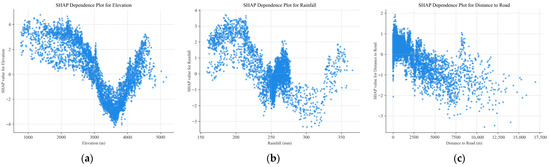
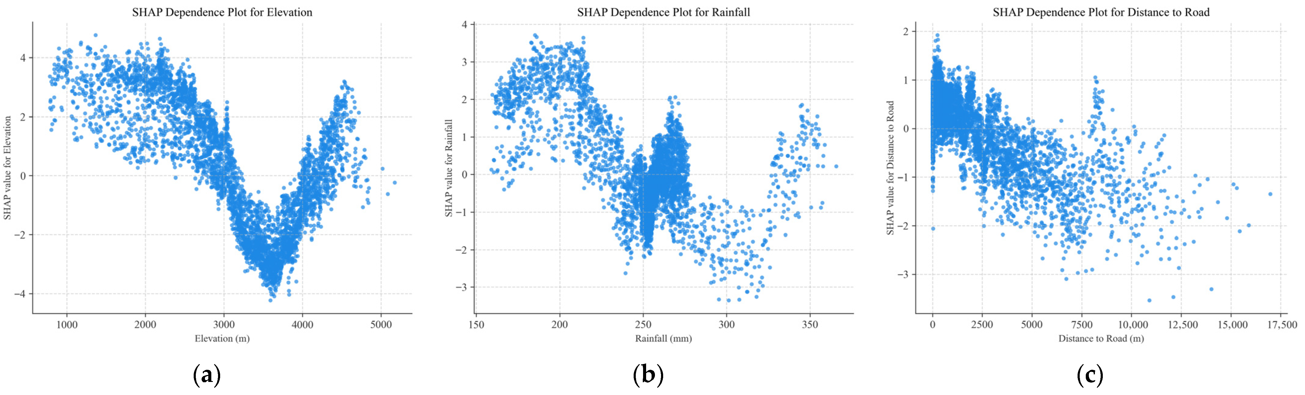
As shown in Figure 17a, the SHAP altitude dependency plot reveals a nonlinear “V-shaped” relationship between SHAP and landslide susceptibility. Within the elevation range of 800–2800 m, SHAP values are relatively high, but as elevation increases, SHAP tends to decrease. This is because in the relatively low-elevation areas of this region, human engineering activities—such as soil erosion or the disruption of surface soil stress—are more frequent, and human activities and river erosion have significantly exacerbated slope instability [79]. Figure 17b shows a complex pattern of rainfall fluctuations, reflecting the stepwise effect of rainfall on landslide triggering. Rainfall in the range of 160–220 mm promotes landslide occurrence; when rainfall exceeds 330 mm, the SHAP value rises rapidly, indicating that the risk of landslides increases linearly with increasing rainfall. Figure 17c shows that distance to road has a clear negative effect on landslide susceptibility. Higher SHAP values are mainly concentrated in areas close to roads, whereas SHAP values decrease progressively with increasing distance, indicating that road-related engineering disturbance plays an important role in promoting landslide occurrence. This result suggests that slope units adjacent to roads are more likely to become unstable under the combined influence of excavation and terrain disturbance.

Figure 17. SHAP dependence plots of factor: (a) Elevation; (b) Rainfall; (c) Distance to road.

In this study, the relatively low resolution of precipitation data may introduce some uncertainty into the modeling of high-mountain canyon regions. Although all control factors were aggregated to the slope unit scale prior to model training, the relatively coarse precipitation data may still smooth out local precipitation variability. Therefore, the precipitation factors in this study should primarily be regarded as regional hydroclimatic background variables rather than precise indicators of micro-scale triggering conditions. Future work will employ higher-resolution precipitation data to further assess the impact of rainfall spatial resolution on landslide susceptibility modeling.

4.2. Negative Landslide Sample Selection

Negative sample selection is a critical but often under-discussed issue in landslide susceptibility modeling, because non-landslide units do not necessarily represent truly stable conditions, but rather areas where no landslide has been identified in the available inventory [80]. Unlike the selection of positive landslide samples, the selection of negative samples is highly subjective, and most existing studies rely on random sampling methods to obtain negative samples.

In this study, negative samples were randomly selected from areas outside a 2 km buffer zone of known landslides to reduce spatial dependence with landslide samples. When using a buffer control strategy to select negative samples, the choice of buffer distance is subjective. For example, Wang et al. excluded a 500 m buffer zone before extracting negative samples [80], Zhu et al. set a 350 m buffer zone to extract missing landslide data [81], while Liu et al.’s study suggested that a buffer zone of less than 3 km is more suitable for Taojiang County [82]. Short buffer zones may lead to the selection of high-susceptibility landslide areas, causing the model to classify high-susceptibility regions as non-landslide samples during training, thus reducing the proportion of high-susceptibility areas. Conversely, long buffer zones reduce the proportion of low-susceptibility areas.

Furthermore, landslides may still occur in these areas in the future, meaning that some negative samples could represent potentially susceptible locations [83,84]. This uncertainty has been highlighted in previous studies, which noted that negative sample selection is one of the major sources of uncertainty in landslide susceptibility modeling, particularly when inventories are incomplete or when future slope failures may occur outside the currently mapped landslide areas.

In addition, we compared negative samples selected from extremely low-risk areas using traditional information value-based prediction methods with the buffer-zone-controlled negative samples used in this study. The results showed that models constructed using negative samples extracted from extremely low-risk areas achieved higher AUC values. This indicates that model performance is highly sensitive to the definition of negative samples, suggesting that the 2 km buffer zone negative sample extraction strategy is not the only optimal solution. In future research, we will focus on conducting an in-depth analysis of the complex issue of landslide negative sample selection, including different buffer distances, various negative sample selection strategies, and their impacts on model performance and interpretability.

4.3. Limitation of the Slope Units

The selection of mapping units plays an important role in landslide susceptibility assessment because it influences how terrain conditions and geomorphological processes are represented. Grid cells have been widely used due to their simplicity and compatibility with raster-based spatial analysis, and they can effectively represent terrain characteristics when appropriate terrain attributes are incorporated. However, in highly dissected mountainous regions, grid cells may intersect natural terrain boundaries such as ridges and valleys, which can fragment geomorphic features [85]. In contrast, slope units are delineated based on topographic segmentation and therefore better approximate natural hillslope boundaries, allowing slope-scale processes to be represented more consistently.

Nevertheless, slope-unit-based approaches also have limitations. The delineation of slope units is sensitive to parameter settings, which can lead to variations in unit size and spatial configuration. Excessively small units may cause unnecessary fragmentation, whereas overly large units may contain heterogeneous environmental conditions. In this study, the standard deviation of slope aspect and the global Moran’s I index were used to evaluate internal homogeneity and spatial autocorrelation of slope units, respectively. The optimal parameter combination was determined by integrating these two indicators, which helps reduce subjectivity in slope unit delineation.

Despite these limitations, the Random Forest model based on optimized slope units achieved good predictive performance (AUC = 0.852). The results suggest that the parameter optimization strategy for slope unit delineation is effective in representing landslide-related terrain characteristics in the study area. This strategy may provide a useful reference for future landslide susceptibility studies in mountainous regions characterized by clear topographic relief, strong environmental heterogeneity, and sufficient landslide inventory and terrain data.

5. Conclusions

This study focuses on landslide susceptibility mapping in a high-mountain gorge region and explores the integrated use of optimized slope units, Random Forest modeling, and SHAP-based interpretation in the Upper Minjiang River. While traditional grid-based units may not fully capture the physical boundaries of landslides in complex terrains like the Upper Minjiang River, this research provides a robust framework by integrating optimized slope units with the Random Forest (RF) model.

Through this study, the following main conclusions and insights were obtained:

• On the eastern edge of the Tibetan Plateau, the upper Minjiang River has created landslide dangers. A total of 3785 landslides, encompassing an area of around 1271 km², were interpreted within the 22,950 km² research region using human–computer interactive interpretation technologies and the Google Earth platform.
• The range of the LAP (landslide area percentage) and LND (landslide number density) is 0 to 5.4% and 0 to 1.89 km⁻², respectively. The landslides are mainly classified into three scales: 9 small landslides, 2989 medium landslides, and 787 large landslides.
• The spatial distribution characteristics of landslide hazards exhibits the following characteristics: concentrated development in high mountain and canyon landforms; distribution along the upper Minjiang River’s main channels, such as the Heishui River and the Zagunao River basin in Li County; and dense distribution along some fault zones, such as the Minjiang Fault Zone, the Wenchuan–Maowen Fault Zone, and the Beichuan–Yingxiu Fault Zone.
• The optimized slope unit was selected by the normalization superposition method. When the parameter combination a = 1 × 10⁵ m² and c = 0.25, the slope aspect standard deviation was 59.661. When the global Moran’s I was 0.11998, the minimum normalization superposition was 0.784, which is the ideal slope unit division result. The study area was divided into 30,513 slope units.
• The optimized slope-unit-based Random Forest model demonstrates strong predictive performance, achieving an AUC value of 0.852 and effectively identifying zones with elevated landslide susceptibility. It is indicated that the selected conditioning factors and mapping units are generally appropriate for regional-scale landslide susceptibility assessment. The susceptibility map further shows that high- and very high-susceptibility zones are mainly concentrated along the main river valleys and in areas strongly affected by tectonic activity and human disturbance.
• The SHAP analysis further indicates that elevation, rainfall, and distance to road are the most important controlling factors in the study area. Their effects suggest that landslide occurrence in the Upper Minjiang River is jointly controlled by regional topographic conditions, hydro-climatic background, and road-related engineering disturbance. This highlights that landslide susceptibility in high-mountain gorge regions is not governed by a single factor, but by the interaction of natural environmental controls and human activities.

Overall, this study provides an application-oriented reference for landslide susceptibility assessment in the Upper Minjiang River and in other mountainous regions with strong terrain relief and complex environmental heterogeneity. In the future research will investigate the impact of selecting landslide negative samples from extremely low- and low-prone areas on model robustness and test the transferability of the slope-unit-based Random Forest framework in other landslide-prone catchments of the eastern Tibetan Plateau, so as to evaluate its broader applicability and support more general regional susceptibility assessment.

References

- Froude, M.J.; Petley, D.N. Global fatal landslide occurrence from 2004 to 2016. Nat. Hazards Earth Syst. Sci. 2018, 18, 2161–2181. [Google Scholar] [CrossRef] [Scilit]
- Petley, D. Global patterns of loss of life from landslides. Geology 2012, 40, 927–930. [Google Scholar] [CrossRef] [Scilit]
- Ávila, G.; Ávila-Guzmán, M.P. Lessons from the Great Gramalote: Colombia Landslide (2010) and its Relocation Process. In Progress in Landslide Research and Technology, Volume 3 Issue 2, 2024; Springer: Berlin/Heidelberg, Germany, 2025; pp. 61–71. [Google Scholar]
- Gizzi, F.; Bentivenga, M.; Lasaponara, R.; Danese, M.; Potenza, M.; Sileo, M.; Masini, N. Natural hazards, human factors, and “ghost towns”: A multi-level approach. Geoheritage 2019, 11, 1533–1565. [Google Scholar] [CrossRef] [Scilit]
- Yin, Y.; Wang, F.; Sun, P. Landslide hazards triggered by the 2008 Wenchuan earthquake, Sichuan, China. Landslides 2009, 6, 139–152. [Google Scholar] [CrossRef] [Scilit]
- Huggel, C.; Clague, J.J.; Korup, O. Is climate change responsible for changing landslide activity in high mountains? Earth Surf. Process. Landf. 2012, 37, 77–91. [Google Scholar] [CrossRef] [Scilit]
- Guzzetti, F. Landslide Hazard and Risk Assessment. Ph.D. Thesis, Universitäts-und Landesbibliothek Bonn, Bonn, Germany, 2006. [Google Scholar]
- Brabb, E.E. Innovative approaches to landslide hazard and risk mapping. In Proceedings 4th International Symposium on Landslides, Toronto; Canadian Geotechnical Society: Toronto, ON, Canada, 1984; Volume 1, pp. 307–323. [Google Scholar]
- Panchal, S.; Shrivastava, A.K. A comparative study of frequency ratio, Shannon’s entropy and analytic hierarchy process (AHP) models for landslide susceptibility assessment. ISPRS Int. J. Geo-Inf. 2021, 10, 603. [Google Scholar] [CrossRef] [Scilit]
- Zhao, H.; Yao, L.; Mei, G.; Liu, T.; Ning, Y. A fuzzy comprehensive evaluation method based on AHP and entropy for a landslide susceptibility map. Entropy 2017, 19, 396. [Google Scholar] [CrossRef] [Scilit]
- Ali, S.A.; Parvin, F.; Vojteková, J.; Costache, R.; Linh, N.T.T.; Pham, Q.B.; Vojtek, M.; Gigović, L.; Ahmad, A.; Ghorbani, M.A. GIS-based landslide susceptibility modeling: A comparison between fuzzy multi-criteria and machine learning algorithms. Geosci. Front. 2021, 12, 857–876. [Google Scholar] [CrossRef] [Scilit]
- Sun, D.; Chen, D.; Zhang, J.; Mi, C.; Gu, Q.; Wen, H. Landslide Susceptibility Mapping Based on Interpretable Machine Learning from the Perspective of Geomorphological Differentiation. Remote Sens. 2023, 12, 1018. [Google Scholar] [CrossRef] [Scilit]
- Aleotti, P.; Chowdhury, R. Landslide hazard assessment: Summary review and new perspectives. Bull. Eng. Geol. Environ. 1999, 58, 21–44. [Google Scholar] [CrossRef] [Scilit]
- Chowdhuri, I.; Pal, S.C.; Arabameri, A.; Saha, A.; Chakrabortty, R.; Blaschke, T.; Pradhan, B.; Band, S.S. Implementation of artificial intelligence based ensemble models for gully erosion susceptibility assessment. Remote Sens. 2020, 12, 3620. [Google Scholar] [CrossRef] [Scilit]
- Chen, W.; Xie, X.; Peng, J.; Shahabi, H.; Hong, H.; Bui, D.T.; Duan, Z.; Li, S.; Zhu, A.-X. GIS-based landslide susceptibility evaluation using a novel hybrid integration approach of bivariate statistical based random forest method. Catena 2018, 164, 135–149. [Google Scholar] [CrossRef] [Scilit]
- Breiman, L. Random forests. Mach. Learn. 2001, 45, 5–32. [Google Scholar] [CrossRef] [Scilit]
- Li, L.; Lan, H. Integration of spatial probability and size in slope-unit-based landslide susceptibility assessment: A case study. Int. J. Environ. Res. Public Health 2020, 17, 8055. [Google Scholar] [CrossRef] [Scilit]
- Chang, Z.; Catani, F.; Huang, F.; Liu, G.; Meena, S.R.; Huang, J.; Zhou, C. Landslide susceptibility prediction using slope unit-based machine learning models considering the heterogeneity of conditioning factors. J. Rock Mech. Geotech. Eng. 2023, 15, 1127–1143. [Google Scholar] [CrossRef] [Scilit]
- Huang, J.; Wen, H.; Zhou, X.; Xiao, J. Is there difference in landslide susceptibility model based on explainable artificial intelligence from the perspective of slope units with different scales? Reliab. Eng. Syst. Saf. 2025, 266, 111701. [Google Scholar] [CrossRef] [Scilit]
- Carrara, A.; Cardinali, M.; Guzzetti, F.; Reichenbach, P. GIS technology in mapping landslide hazard. In Geographical Information Systems in Assessing Natural Hazards; Springer: Berlin/Heidelberg, Germany, 1995; pp. 135–175. [Google Scholar]
- Camilo, D.C.; Lombardo, L.; Mai, P.M.; Dou, J.; Huser, R. Handling high predictor dimensionality in slope-unit-based landslide susceptibility models through LASSO-penalized Generalized Linear Model. Environ. Model. Softw. 2017, 97, 145–156. [Google Scholar] [CrossRef] [Scilit]
- Bell, R.; Glade, T. Quantitative risk analysis for landslides–Examples from Bíldudalur, NW-Iceland. Nat. Hazards Earth Syst. Sci. 2004, 4, 117–131. [Google Scholar] [CrossRef] [Scilit]
- Alvioli, M.; Guzzetti, F.; Marchesini, I. Parameter-free delineation of slope units and terrain subdivision of Italy. Geomorphology 2020, 358, 107124. [Google Scholar] [CrossRef] [Scilit]
- Reichenbach, P.; Rossi, M.; Malamud, B.D.; Mihir, M.; Guzzetti, F. A review of statistically-based landslide susceptibility models. Earth-Sci. Rev. 2018, 180, 60–91. [Google Scholar] [CrossRef] [Scilit]
- Xia, D.; Tang, H.; Glade, T.; Tang, C.; Wang, Q. KNN-GCN: A deep learning approach for slope-unit-based landslide susceptibility mapping incorporating spatial correlations. Math. Geosci. 2024, 56, 1011–1039. [Google Scholar] [CrossRef] [Scilit]
- Shao, X.; Xu, C.; Ma, S. Coseismic Landslide Area Prediction Using Generalised Additive Model: A Case Study of the 2013 Minxian Earthquake. Geosci. Data J. 2026, 13, e70041. [Google Scholar] [CrossRef] [Scilit]
- Wang, X.; Li, Y.; Yuan, Y.; Zhou, Z.; Wang, L. Palaeoclimate and palaeoseismic events discovered in Diexi barrier lake on the Minjiang River, China. Nat. Hazards Earth Syst. Sci. 2014, 14, 2069–2078. [Google Scholar] [CrossRef] [Scilit]
- Lin, L.; Chen, G.; Shi, W.; Jin, J.; Wu, J.; Huang, F.; Chong, Y.; Meng, Y.; Li, Y.; Zhang, Y. Spatiotemporal Evolution Pattern and Driving Mechanisms of Landslides in the Wenchuan Earthquake-Affected Region: A Case Study in the Bailong River Basin, China. Remote Sens. 2022, 14, 2339. [Google Scholar] [CrossRef] [Scilit]
- Ma, J.; Chen, J.; Cui, Z.; Zhou, W.; Liu, C.; Guo, P.; Shi, Q. Sedimentary evidence of outburst deposits induced by the Diexi paleolandslide-dammed lake of the upper Minjiang River in China. Quat. Int. 2018, 464, 460–481. [Google Scholar] [CrossRef] [Scilit]
- Gao, H.; Xu, C.; Xie, C.; Ma, J.; Xiao, Z. Landslides triggered by the July 2023 extreme rainstorm in the Haihe River Basin, China. Landslides 2024, 21, 2885–2890. [Google Scholar] [CrossRef] [Scilit]
- Wang, J. Long-term trend of runoff in Minjiang basin and its respomes to climate change over Tibetan Plateau. Resour. Environ. Yangtze Basin 2010, 19, 933–939. [Google Scholar]
- Geng, C.; Xu, C.; Li, L.; Gao, H. Landslide Inventory Mapping in the Upper Minjiang River, Eastern Tibetan Plateau, Using Multi-Source Satellite Remote Sensing. Trans. GIS 2025, 29, e70165. [Google Scholar] [CrossRef] [Scilit]
- Wu, X.; Xu, X.; Yu, G.; Ren, J.; Yang, X.; Chen, G.; Xu, C.; Du, K.; Huang, X.; Yang, H. The China Active Faults Database (CAFD) and its web system. Earth Syst. Sci. Data 2024, 16, 3391–3417. [Google Scholar] [CrossRef] [Scilit]
- Xu, C.; Xu, X.; Dai, F.; Wu, Z.; He, H.; Shi, F.; Wu, X.; Xu, S. Application of an incomplete landslide inventory, logistic regression model and its validation for landslide susceptibility mapping related to the May 12, 2008 Wenchuan earthquake of China. Nat. Hazards 2013, 68, 883–900. [Google Scholar] [CrossRef] [Scilit]
- Yi, Y.; Zhang, Z.; Zhang, W.; Xu, Q.; Deng, C.; Li, Q. GIS-based earthquake-triggered-landslide susceptibility mapping with an integrated weighted index model in Jiuzhaigou region of Sichuan Province, China. Nat. Hazards Earth Syst. Sci. 2019, 19, 1973–1988. [Google Scholar] [CrossRef] [Scilit]
- Chai, H.; Liu, H.; Zhang, Z. The 1933 Daxi Earthquake Landslide River Blockage Event and Its Environmental Effects. J. Geol. Hazards Environ. Preserv. 1995, 6, 7–17. [Google Scholar]
- Jones, L.M.; Han, W.; Hauksson, E.; Jin, A.; Zhang, Y.; Luo, Z. Focal mechanisms and aftershock locations of the Songpan earthquakes of August 1976 in Sichuan, China. J. Geophys. Res. Solid Earth 1984, 89, 7697–7707. [Google Scholar] [CrossRef] [Scilit]
- Dai, F.C.; Xu, C.; Yao, X.; Xu, L.; Tu, X.B.; Gong, Q.M. Spatial distribution of landslides triggered by the 2008 Ms 8.0 Wenchuan earthquake, China. J. Asian Earth Sci. 2011, 40, 883–895. [Google Scholar] [CrossRef] [Scilit]
- Ma, J.; Gao, H.; Xu, C.; Qi, S. Characterization and formation mechanism of the catastrophic flash flood-debris flow hazard triggered by the July 2023 extreme rainstorm in Hantai Gully of Beijing, China. Landslides 2025, 22, 877–893. [Google Scholar] [CrossRef] [Scilit]
- Qi, W.; Wei, M.; Yang, W.; Xu, C.; Ma, C. Automatic mapping of landslides by the ResU-Net. Remote Sens. 2020, 12, 2487. [Google Scholar] [CrossRef] [Scilit]
- Xu, C.; Xu, X.; Yao, X.; Dai, F. Three (nearly) complete inventories of landslides triggered by the May 12, 2008 Wenchuan Mw 7.9 earthquake of China and their spatial distribution statistical analysis. Landslides 2014, 11, 441–461. [Google Scholar] [CrossRef] [Scilit]
- Xu, Q.; Zhao, B.; Dai, K.; Dong, X.; Li, W.; Zhu, X.; Yang, Y.; Xiao, X.; Wang, X.; Huang, J. Remote sensing for landslide investigations: A progress report from China. Eng. Geol. 2023, 321, 107156. [Google Scholar] [CrossRef] [Scilit]
- Fiorucci, F.; Ardizzone, F.; Mondini, A.C.; Viero, A.; Guzzetti, F. Visual interpretation of stereoscopic NDVI satellite images to map rainfall-induced landslides. Landslides 2019, 16, 165–174. [Google Scholar] [CrossRef] [Scilit]
- Xu, C. Preparation of earthquake-triggered landslide inventory maps using remote sensing and GIS technologies: Principles and case studies. Geosci. Front. 2015, 6, 825–836. [Google Scholar] [CrossRef] [Scilit]
- Xu, C.; Xu, X.; Shyu, J.B.H. Database and spatial distribution of landslides triggered by the Lushan, China Mw 6.6 earthquake of 20 April 2013. Geomorphology 2015, 248, 77–92. [Google Scholar] [CrossRef] [Scilit]
- Ma, S.; Shao, X.; Xu, C.; Niu, P. Geometry and mobility characteristics of landslides triggered by the 2018 Mw 7.5 Palu earthquake in Indonesia: S. Ma et al. Landslides 2025, 22, 3973–3988. [Google Scholar] [CrossRef] [Scilit]
- Guzzetti, F.; Mondini, A.C.; Cardinali, M.; Fiorucci, F.; Santangelo, M.; Chang, K.-T. Landslide inventory maps: New tools for an old problem. Earth-Sci. Rev. 2012, 112, 42–66. [Google Scholar] [CrossRef] [Scilit]
- Huang, Y.; Xu, C.; He, X.; Cheng, J.; Huang, Y.; Wu, L.; Xu, X. Distribution characteristics and cumulative effects of landslides triggered by multiple moderate-magnitude earthquakes: A case study of the comprehensive seismic impact area in Yibin, Sichuan, China. Landslides 2024, 21, 2927–2943. [Google Scholar] [CrossRef] [Scilit]
- Ma, S.; Shao, X.; Xu, C. Estimating the quality of the most popular machine learning algorithms for landslide susceptibility mapping in 2018 Mw 7.5 Palu earthquake. Remote Sens. 2023, 15, 4733. [Google Scholar] [CrossRef] [Scilit]
- Huang, Y.; Xu, C.; Li, L.; He, X.; Cheng, J.; Xu, X.; Li, J.; Zhang, X. Inventory and Spatial Distribution of Ancient Landslides in Hualong County, China. Land 2023, 12, 136. [Google Scholar] [CrossRef] [Scilit]
- Tien Bui, D.; Pradhan, B.; Lofman, O.; Revhaug, I. Landslide susceptibility assessment in vietnam using support vector machines, decision tree, and Naive Bayes Models. Math. Probl. Eng. 2012, 2012, 974638. [Google Scholar] [CrossRef] [Scilit]
- Shao, X.; Ma, S.; Xu, C. Distribution and characteristics of shallow landslides triggered by the 2018 Mw 7.5 Palu earthquake, Indonesia. Landslides 2023, 20, 157–175. [Google Scholar] [CrossRef] [Scilit]
- Silverman, B.W. Density Estimation for Statistics and Data Analysis; Routledge: London, UK, 2018. [Google Scholar]
- Tezel, D.; Inam, S.; Kocaman, S. GIS-Based Assessment of Habitat Networks for Conservation Planning in Kas-Kekova Protected Area (Turkey). ISPRS Int. J. Geo-Inf. 2020, 9, 91. [Google Scholar] [CrossRef] [Scilit]
- Parker, R.N.; Densmore, A.L.; Rosser, N.J.; De Michele, M.; Li, Y.; Huang, R.; Whadcoat, S.; Petley, D.N. Mass wasting triggered by the 2008 Wenchuan earthquake is greater than orogenic growth. Nat. Geosci. 2011, 4, 449–452. [Google Scholar] [CrossRef] [Scilit]
- Larsen, I.J.; Montgomery, D.R.; Korup, O. Landslide erosion controlled by hillslope material. Nat. Geosci. 2010, 3, 247–251. [Google Scholar] [CrossRef] [Scilit]
- McColl, S.T.; Cook, S.J. A universal size classification system for landslides. Landslides 2025, 62, 118. [Google Scholar] [CrossRef] [Scilit]
- Varnes, D. Slope movement types and processes. Landslides Anal. Control 1978, 176, e33. [Google Scholar]
- Liao, M.; Wen, H.; Yang, L. Identifying the essential conditioning factors of landslide susceptibility models under different grid resolutions using hybrid machine learning: A case of Wushan and Wuxi counties, China. Catena 2022, 217, 106428. [Google Scholar] [CrossRef] [Scilit]
- Alvioli, M.; Marchesini, I.; Reichenbach, P.; Rossi, M.; Ardizzone, F.; Fiorucci, F.; Guzzetti, F. Automatic delineation of geomorphological slope units with r. slopeunits v1. 0 and their optimization for landslide susceptibility modeling. Geosci. Model Dev. 2016, 9, 3975–3991. [Google Scholar] [CrossRef] [Scilit]
- Rossi, M.; Guzzetti, F.; Reichenbach, P.; Mondini, A.C.; Peruccacci, S. Optimal landslide susceptibility zonation based on multiple forecasts. Geomorphology 2010, 114, 129–142. [Google Scholar] [CrossRef] [Scilit]
- Guzzetti, F.; Carrara, A.; Cardinali, M.; Reichenbach, P. Landslide hazard evaluation: A review of current techniques and their application in a multi-scale study, Central Italy. Geomorphology 1999, 31, 181–216. [Google Scholar] [CrossRef] [Scilit]
- Chen, X.; Chen, W. GIS-based landslide susceptibility assessment using optimized hybrid machine learning methods. Catena 2021, 196, 104833. [Google Scholar] [CrossRef] [Scilit]
- Liu, J.; Xu, C.; Zhao, B.; Yang, Z.; Liu, Y.; Zhang, S.; Kong, X.; Lan, Q.; Xu, W.; Qi, W. Deformation Slope Extraction and Influencing Factor Analysis Using LT-1 Satellite Data: A Case Study of Chongqing and Surrounding Areas, China. Remote Sens. 2025, 17, 156. [Google Scholar] [CrossRef] [Scilit]
- Trigila, A.; Iadanza, C.; Esposito, C.; Scarascia-Mugnozza, G. Comparison of Logistic Regression and Random Forests techniques for shallow landslide susceptibility assessment in Giampilieri (NE Sicily, Italy). Geomorphology 2015, 249, 119–136. [Google Scholar] [CrossRef] [Scilit]
- Huang, F.; Mao, D.; Jiang, S.-H.; Zhou, C.; Fan, X.; Zeng, Z.; Catani, F.; Yu, C.; Chang, Z.; Huang, J. Uncertainties in landslide susceptibility prediction modeling: A review on the incompleteness of landslide inventory and its influence rules. Geosci. Front. 2024, 15, 101886. [Google Scholar] [CrossRef] [Scilit]
- Frattini, P.; Crosta, G.; Carrara, A. Techniques for evaluating the performance of landslide susceptibility models. Eng. Geol. 2010, 111, 62–72. [Google Scholar] [CrossRef] [Scilit]
- Lundberg, S.M.; Lee, S.-I. A unified approach to interpreting model predictions. Adv. Neural Inf. Process. Syst. 2017, 30, 4768–4777. [Google Scholar]
- Cui, S.; Wu, H.; Pei, X.; Yang, Q.; Huang, R.; Guo, B. Characterizing the spatial distribution, frequency, geomorphological and geological controls on landslides triggered by the 1933 Mw 7.3 Diexi Earthquake, Sichuan, China. Geomorphology 2022, 403, 108177. [Google Scholar] [CrossRef] [Scilit]
- Wang, Y.; Li, Y. Analysis on the controlling factor of formation of landslides and avalanches in Manaoding-Lianghekou, upper reaches of Minjiang. J. Chengdu Univ. Technol. (Sci. Technol. Ed.) 2000, 27, 205–208. [Google Scholar]
- Fan, X.; Xu, Q.; Scaringi, G.; Dai, L.; Li, W.; Dong, X.; Zhu, X.; Pei, X.; Dai, K.; Havenith, H.-B. Failure mechanism and kinematics of the deadly June 24th 2017 Xinmo landslide, Maoxian, Sichuan, China. Landslides 2017, 14, 2129–2146. [Google Scholar] [CrossRef] [Scilit]
- Liu, Z.; Su, L.; Zhang, C.; Iqbal, J.; Hu, B.; Dong, Z. Investigation of the dynamic process of the Xinmo landslide using the discrete element method. Comput. Geotech. 2020, 123, 103561. [Google Scholar] [CrossRef] [Scilit]
- Tang, C.; Tang, J.; van Westen, C.J.; Han, J.; Mavrouli, O.; Tang, C. Modeling landslide failure surfaces by polynomial surface fitting. Geomorphology 2020, 368, 107358. [Google Scholar] [CrossRef] [Scilit]
- Leong, E.-C.; Cheng, Z. A geometry-modeling method to estimate landslide volume from source area. Landslides 2022, 19, 1971–1985. [Google Scholar] [CrossRef] [Scilit]
- Wei, C.; Zhang, Y.; Feng, W.; Liao, W. Analysis of intensity and regularity of geohazards in upper reaches of Minjiang River. J. Eng. Geol. 2019, 27, 640–650. [Google Scholar] [CrossRef]
- Wu, R. Research on Reactivation Mechanism and Hazard Assessment of Ancient Landslide in Upper Reaches of Minjiang River; Chinese Academy of Geological Sciences: Beijing, China, 2019. [Google Scholar]
- Zhong, Y. The Development and Distribution of Ancient Landslides in the Upstream of the Minjiang River and Their Long-Term Effects on the Evolution of Rivers; Chengdu University of Technology: Chengdu, China, 2023. [Google Scholar]
- Bornaetxea, T.; Rossi, M.; Marchesini, I.; Alvioli, M. Effective surveyed area and its role in statistical landslide susceptibility assessments. Nat. Hazards Earth Syst. Sci. Discuss. 2018, 18, 2455–2469. [Google Scholar] [CrossRef] [Scilit]
- Wang, X.; Bai, S. Landslide susceptibility mapping and interpretation in the upper Minjiang river basin. Remote Sens. 2023, 15, 4947. [Google Scholar] [CrossRef] [Scilit]
- Wang, J.; Wang, Y.; Li, M.; Qi, Z.; Li, C.; Qi, H.; Zhang, X. Improved landslide susceptibility assessment: A new negative sample collection strategy and a comparative analysis of zoning methods. Ecol. Indic. 2024, 169, 112948. [Google Scholar] [CrossRef] [Scilit]
- Zhu, A.X.; Miao, Y.; Liu, J.; Bai, S.; Zeng, C.; Ma, T.; Hong, H. A similarity-based approach to sampling absence data for landslide susceptibility mapping using data-driven methods. Catena 2019, 183, 104188. [Google Scholar] [CrossRef] [Scilit]
- Liu, L.-L.; Xiao, H.; Zhang, Y.-L.; Yang, C. An improved buffer-controlled sampling strategy for landslide susceptibility assessment considering the spatial heterogeneity of conditioning factors. Bull. Eng. Geol. Environ. 2024, 83, 512. [Google Scholar] [CrossRef] [Scilit]
- Khabiri, S.; Crawford, M.M.; Koch, H.J.; Haneberg, W.C.; Zhu, Y. An assessment of negative samples and model structures in landslide susceptibility characterization based on Bayesian network models. Remote Sens. 2023, 15, 3200. [Google Scholar] [CrossRef] [Scilit]
- Fu, X.; Liu, Y.; Zhu, Q.; Ge, D.; Li, Y.; Zeng, H. Reliable assessment approach of landslide susceptibility in broad areas based on optimal slope units and negative samples involving priori knowledge. Int. J. Digit. Earth 2022, 15, 2495–2510. [Google Scholar] [CrossRef] [Scilit]
- Ba, Q.; Chen, Y.; Deng, S.; Yang, J.; Li, H. A comparison of slope units and grid cells as mapping units for landslide susceptibility assessment. Earth Sci. Inform. 2018, 11, 373–388. [Google Scholar] [CrossRef] [Scilit]
Disclaimer/Publisher’s Note: The statements, opinions and data contained in all publications are solely those of the individual author(s) and contributor(s) and not of MDPI and/or the editor(s). MDPI and/or the editor(s) disclaim responsibility for any injury to people or property resulting from any ideas, methods, instructions or products referred to in the content. |
© 2026 by the authors. Licensee MDPI, Basel, Switzerland. This article is an open access article distributed under the terms and conditions of the Creative Commons Attribution (CC BY) license.