Digital Soil Mapping of Soil Organic Carbon in Smallholder Robusta Coffee Landscapes of South–Central Uganda

Abstract

Reliable spatial information on soil organic carbon (SOC) is important for soil-fertility management, climate-resilient coffee production, and land-restoration planning, yet the heterogeneity of smallholder agricultural landscapes is difficult to represent with field observations alone. This study characterised SOC variability, compared four machine-learning (ML) algorithms—Random Forest (RF), Cubist, Gradient Boosted Machines (GBM), and Support Vector Machine (SVM)—identified the main predictive environmental covariates, and generated SOC prediction maps for a smallholder Robusta coffee landscape in South–Central Uganda. A total of 126 georeferenced surface-soil observations (0–30 cm) were analysed for SOC using the Walkley–Black dichromate wet-oxidation method and related to climatic, terrain, spectral, soil, land-cover, and spatial-position covariates within the SCORPAN framework. Models were tuned within an SOC-stratified training subset and evaluated using a withheld 20% random holdout. Observed SOC ranged from 0.31% to 5.30%, with a mean of 2.06% and a coefficient of variation of 62.7%. Independent holdout performance was limited. SVM performed best (R² = 0.36; RMSE = 1.05), followed by Cubist, RF, and GBM. Annual mean temperature and spatial position had the highest predictive importance, followed by soil type, Landsat 9 Band 5, and annual precipitation. All four models reproduced a broad pattern of relatively higher SOC in Kalungu and central Masaka and lower SOC in Southern Kyotera and parts of Lwengo, although the magnitude of local variation differed among algorithms. The resulting maps are, therefore, best suited for landscape-level screening, sampling prioritisation, and identifying areas requiring field verification, rather than farm-level SOC prescription.

1. Introduction

Soil organic carbon (SOC) is spatially heterogeneous because it reflects the balance between organic-carbon inputs and losses, as well as the interaction of soil-forming and management processes. Carbon inputs arise from litter, roots, crop residues, and organic amendments, whereas decomposition, erosion, leaching, and biomass removal contribute to carbon losses. Climate, topography, hydrology, parent material, soil properties, land use, management, and management history influence these processes [1,2,3,4]. Consequently, locations with similar regional climates may still have markedly different SOC concentrations at farm and landscape scales.

Across Sub-Saharan Africa, intensive cultivation, soil erosion, vegetation loss, and inadequate replenishment of soil organic matter have contributed to declining soil quality and substantial within- and between-farm variability [5,6]. Spatially explicit soil information is, therefore, useful for identifying areas where SOC depletion may be more likely, targeting additional soil sampling, and directing restoration or soil-management interventions more efficiently.

Ugandan soil assessments have documented substantial variations in organic matter, pH, macronutrients, texture, and related soil properties across major agricultural and coffee-growing regions [7,8]. Soil fertility constraints, erosion, and management differences are also reported in Central and South–Central Uganda [9,10,11]. Smallholder Robusta coffee farms are particularly heterogeneous because they differ in shade-tree density, banana and food-crop integration, canopy structure, residue retention, manure use, and other management practices [12,13]. Most Uganda-specific studies, however, describe conditions at sampled plots or compare management systems; they do not provide continuous, landscape-scale predictions of SOC within fragmented smallholder Robusta coffee areas.

Conventional soil surveys and laboratory analyses provide direct and indispensable measurements, but dense sampling across large and fragmented smallholder landscapes is costly and labour-intensive. Global and regional digital soil products partly address this limitation by providing continuous soil-property estimates [14,15], but their spatial scale and generalised calibration may smooth local variation among farms, terrain positions, soil classes, and land-use configurations. Locally measured soil observations combined with landscape-specific environmental covariates can, therefore, complement broader soil products where finer spatial screening is required.

Digital Soil Mapping (DSM) provides a quantitative framework for relating measured soil properties to spatially continuous environmental covariates and extending those relationships to unsampled locations [2]. The SCORPAN framework represents a soil property as a function of existing soil information (S), climate (C), organisms or vegetation (O), relief (R), parent material (P), age or time (A), and spatial position (N) [2]. Machine-learning approaches are increasingly used in DSM because they can accommodate nonlinear relationships and interactions among diverse covariates [4,16,17]. Their performance is nevertheless dependent on the landscape, sampling design, predictor quality, and model configuration, making transparent comparison and validation essential.

The four algorithms evaluated in this study represent contrasting predictive structures. RF averages many regression trees generated from bootstrap samples and random predictor subsets [18]. GBM sequentially fits trees to reduce residual prediction error [19]. Cubist combines rule-based partitioning with local linear models, and radial SVM represents nonlinear relationships in multidimensional predictor space [20]. Comparing these algorithms under a common training and evaluation framework shows how model structure affects SOC prediction in a heterogeneous smallholder landscape.

The novelty of this study lies not in proposing a new ML algorithm, but in applying a field-calibrated, landscape-specific DSM framework to a data-scarce smallholder Robusta coffee environment in South–Central Uganda. Existing Uganda studies have characterised coffee-region soils and SOC under selected production systems [7,11,21], but comparative evidence on RF, Cubist, GBM, and SVM for continuous SOC mapping within a fragmented Robusta coffee landscape remains limited. The study also examines the relative contribution of climate, terrain, remotely sensed vegetation information, mapped soil and land cover, and spatial position within one common modelling framework.

Accordingly, this study aimed to (1) characterise the variability of field-measured SOC in the study landscape; (2) compare the predictive performance of RF, Cubist, GBM, and SVM; (3) identify the covariates contributing most strongly to SOC prediction while distinguishing predictive importance from causality; and (4) generate continuous SOC prediction surfaces and quantify the degree of disagreement among the four algorithms. The maps are intended as landscape-level screening products rather than substitutes for plot-level soil testing.

2. Materials and Methods

2.1. Study Area

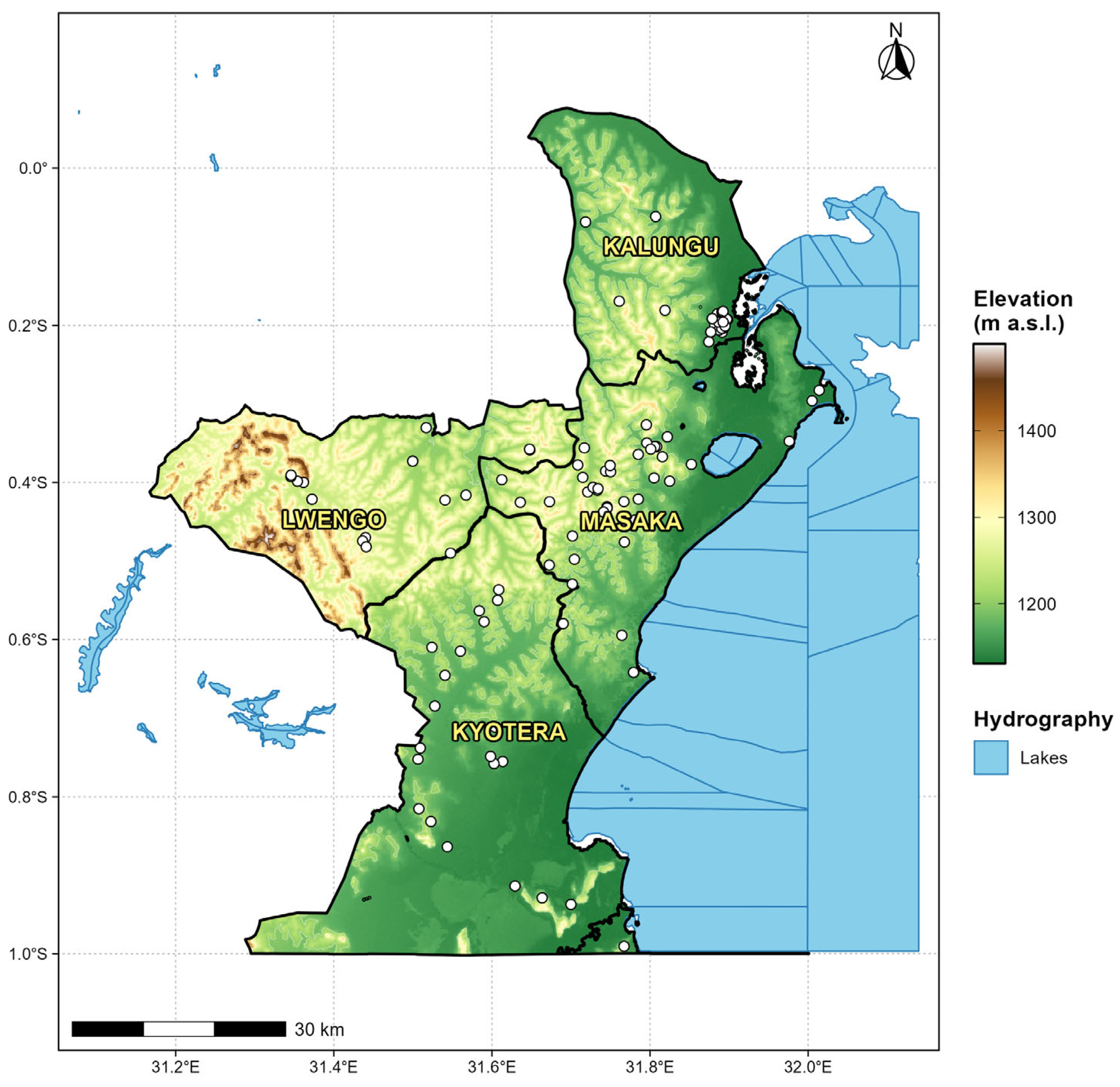
The study was conducted in the Robusta coffee-growing landscape of Greater Masaka in South–Central Uganda, covering Masaka, Kalungu, Lwengo, and Kyotera districts (Figure 1). The area lies largely within the Lake Victoria Crescent, one of Uganda’s principal Robusta coffee-producing zones. Smallholder farming predominates, and coffee is commonly integrated with banana, food crops, fruit trees, and shade or multipurpose trees.

Figure 1. Study area map showing soil sampling locations as white dots against the elevation range of the study area.

The study area has a tropical bimodal rainfall regime, with the main rainfall seasons generally occurring from March to May/June and from September to November, separated by comparatively drier periods. Annual rainfall is commonly about 1400–1600 mm, while the mean temperatures are approximately 22–28 °C, with local and interannual variation [22].

The landscape comprises rolling hills, valley bottoms, wetlands, and relatively level cultivated areas. Soil surveys in South–Central Uganda describe strongly weathered red Ferralsols, along with Phaeozems and black–stony soil units, in parts of the Masaka landscape [8,11]. These soils occur on old, weathered surfaces developed largely over Precambrian basement materials, including granite, gneiss, amphibolite, and quartzite [8]. The resulting variation in weathering, texture, mineralogy, drainage, and landscape position can influence SOC stabilisation and redistribution. Land cover is dominated by smallholder coffee and banana systems, mixed annual cropping, grassland, wetlands, settlements, and remnant natural or semi-natural vegetation.

2.2. Soil Sampling and SOC Determination

Soil observations used for the DSM were obtained from a broader field survey of smallholder Robusta coffee farms undertaken between June and August 2024. Sampling locations were selected to represent variation in coffee-growing environments, soils, vegetation, and prevailing coffee-production systems. Candidate farms were identified with support from farmer lists, farmer organisations, and local coffee networks, and field selection aimed for reasonable spatial dispersion, subject to farm access and the presence of suitable coffee systems. The resulting 126 DSM locations were, therefore, field-based farm observations, rather than points from a regular spatial grid. The sampling density was consequently uneven across the four-district study area. This limitation is considered explicitly when interpreting the maps and validation results.

Within each selected farm or location, a representative sampling area was identified away from features likely to produce atypical soil conditions, including field boundaries, roads and footpaths, termite mounds, manure heaps, drainage channels, and recently disturbed ground. Surface litter was carefully removed before collection. Soil was sampled from 0–30 cm using an 8.3 cm-diameter auger at one central point and three surrounding subsampling points approximately 5 m apart. The four subsamples were combined and thoroughly mixed to form a composite sample of approximately 500 g, thereby reducing the influence of microscale variability. Samples were placed in labelled bags bearing a unique identification code, sampling date, depth, and location. Sampling tools were cleaned between locations to minimise cross-contamination, and coordinates were recorded using a Garmin GPSMAP 65S handheld receiver (Garmin International, Inc., Olathe, KS, USA).

In the laboratory, samples were air-dried at room temperature, gently crushed, and passed through a 2 mm sieve to remove stones, roots, and other coarse materials. SOC concentration was determined using the Walkley–Black dichromate wet-oxidation method following standard soil analytical procedures [23]. A measured soil mass was oxidised with potassium dichromate and concentrated sulphuric acid, and the residual dichromate was back-titrated using standardised ferrous ammonium sulphate and a redox indicator. Laboratory quality assurance and quality control included cleaned analytical glassware and equipment, standardisation/calibration of the relevant reagents or instruments, reagent blanks within analytical batches, and duplicate analysis of selected samples to assess analytical repeatability. Laboratory control or reference materials were used where available, and samples were reanalysed when quality-control checks fell outside the laboratory’s acceptance criteria. Laboratory results were recorded against unique sample-identification codes and cross-checked with field records before use in the modelling dataset.

2.3. Environmental Covariates

Environmental predictors were selected within the SCORPAN framework [2] to represent relief, climate, organisms/vegetation, mapped soil and parent-material information, land cover, and spatial position. Table 1 reports the source, temporal basis, and native spatial resolution of each covariate. The datasets were not fully co-temporal: field SOC was sampled in 2024, the Landsat 9 scenes were acquired in 2025, land-cover data represented 2017 conditions, WorldClim represented long-term climate normals, and the DEM and legacy soil map represented comparatively static landscape properties. These layers were, therefore, treated as environmental proxies rather than observations acquired at the time of soil sampling.

Table 1. Environmental covariates considered for landscape-scale SOC prediction, including data origin, temporal basis, and native spatial resolution.

Covariate Group	Covariate	Source and Temporal Basis	Native Spatial Resolution
Terrain	DEM	SRTM 1 Arc-Second Global DEM; acquired February 2000	~30 m
Terrain	Slope	Derived from the SRTM DEM using WhiteboxTools; based on 2000 DEM	~30 m
Terrain	Profile curvature	Derived from the SRTM DEM using WhiteboxTools; based on 2000 DEM	~30 m
Terrain	Plan curvature	Derived from the SRTM DEM using WhiteboxTools; based on 2000 DEM	~30 m
Terrain	Hillshade	Derived from the SRTM DEM using WhiteboxTools; based on 2000 DEM	~30 m
Terrain	Flow accumulation	Derived from the SRTM DEM using WhiteboxTools; based on 2000 DEM	~30 m
Climate	BIO1 (annual mean temperature)	WorldClim v2.1; 1970–2000 climate normal	30 arc-sec (~1 km)
Climate	BIO12 (annual precipitation)	WorldClim v2.1; 1970–2000 climate normal	30 arc-sec (~1 km)
Vegetation/spectral	NDVI	Derived from Landsat 9 OLI-2 Collection 2 Level-2 Surface Reflectance (Bands 4 and 5); acquired 31 July 2025	30 m
Vegetation/spectral	SAVI	Derived from Landsat 9 OLI-2 Collection 2 Level-2 Surface Reflectance (Bands 4 and 5); acquired 31 July 2025	30 m
Vegetation/spectral	Band 5 (NIR)	Landsat 9 OLI-2 Collection 2 Level-2 Surface Reflectance; acquired 31 July 2025	30 m
Soil/parent material	Soil type	Uganda national legacy soil polygon dataset (UG_SOILS); FAO soil classes; static legacy layer, original survey date not encoded in supplied data	Vector polygons; rasterised to ~30 m grid
Land use/land cover	LULC	National Forestry Authority/UG_LANDUSES; 2017 land-cover layer	Vector polygons; rasterised to ~30 m grid
Spatial position	Easting	Generated from WGS 84/UTM Zone 36S modelling grid; non-temporal	~30 m modelling grid
Spatial position	Northing	Generated from WGS 84/UTM Zone 36S modelling grid; non-temporal	~30 m modelling grid

2.3.1. Terrain Covariates

Elevation was represented using the Shuttle Radar Topography Mission (SRTM) 1 Arc-Second Global DEM, with a native resolution of approximately 30 m. Slope, profile curvature, plan curvature, hillshade, and flow accumulation were derived from the DEM using WhiteboxTools. These terrain attributes were included as proxies for relief-related variations in runoff, erosion and deposition, drainage, moisture redistribution, and solar exposure. Hillshade was used as an indirect representation of differences in terrain illumination and associated microclimatic conditions, rather than as a direct soil-forming variable.

2.3.2. Climatic Covariates

Long-term climate was represented by annual mean temperature (BIO1) and annual precipitation (BIO12) from WorldClim version 2.1 at 30 arc seconds (approximately 1 km), representing the 1970–2000 climatic baseline [24]. These variables were included because temperature and precipitation influence vegetation productivity, soil moisture, microbial activity, decomposition, leaching, and erosion. The WorldClim layers were resampled to the common modelling grid for spatial alignment; this operation improved grid compatibility but did not create climatic information at a finer effective resolution than the original product.

2.3.3. Vegetation Covariates

Vegetation and spectral conditions were represented using Landsat 9 OLI-2 Collection 2 Level-2 Surface Reflectance imagery acquired on 31 July 2025. Surface-reflectance values were scaled according to the Collection 2 Level-2 product specification before index calculation. The Normalised Difference Vegetation Index (NDVI) and Soil-Adjusted Vegetation Index (SAVI) were derived from the red (Band 4) and near-infrared (Band 5) bands as proxies for vegetation greenness and cover. Landsat 9 Band 5 was also considered as an individual spectral predictor. The one-year difference between the 2024 field sampling and the 2025 satellite acquisition is acknowledged as a potential source of temporal mismatch, particularly where vegetation or management changed between dates.

NDVI was calculated as:

$$NDVI={\displaystyle \frac{B5-B4}{B5+B4}}$$

(1)

The Soil-Adjusted Vegetation Index (SAVI) was calculated as:

$$SAVI=\left({\displaystyle \frac{B5-B4}{B5+B4+L}}\right)(1+L)$$

(2)

where:

B5 = Near-Infrared (NIR) band;

B4 = Red band;

L = soil-background adjustment factor (commonly set to 0.5 for areas with moderate vegetation cover).

2.3.4. Soil and Land-Cover Covariates

Mapped soil information was obtained from Uganda’s national legacy soil polygon dataset, in which soil units were represented by FAO soil classes. The polygons were rasterised and included as a categorical predictor to represent broad differences in soil-forming material, texture, mineralogy, drainage, and paedogenic history. Land use and land cover were obtained from the National Forestry Authority/UG_LANDUSES 2017 polygon dataset and were likewise rasterised as a categorical predictor. These broad mapped classes do not resolve farm-level practices, such as manure application, mulching, tillage, coffee age, shade-tree density, or land-use history. No separate age/time predictor was included because a spatially complete land-use history dataset was unavailable.

2.4. Spatial Data Pre-Processing and Harmonisation

All environmental layers were projected to a common WGS 84/UTM Zone 36S coordinate system and harmonised to the SRTM-derived modelling grid at approximately 30 m resolution, with a common extent, origin, and cell alignment. Continuous raster variables were resampled using bilinear interpolation, whereas categorical soil and land-cover layers were rasterised/resampled using nearest-neighbour procedures to preserve class identity. Easting and Northing raster layers were generated from the projected modelling grid to represent the SCORPAN spatial-position factor (N). These coordinates were included to capture the broad residual geographical gradients not fully represented by the environmental covariates. They were not interpreted as direct soil-forming processes, and their use limits extrapolation beyond the study landscape.

SOC values and covariate values were extracted at each sampling location to form the modelling dataset. Predictor screening checked for missing or non-finite values, near-zero variance, and anomalous values. Feature screening was based on the training subset to avoid using the independent test data during model development. The final retained dataset contained 126 complete observations.

2.5. Multicollinearity Assessment and Feature Selection

Pearson correlation analysis assessed redundancy among continuous predictors within the training subset. Predictor pairs with |r| > 0.80 were treated as highly correlated, and redundant variables were removed before model fitting. Selection among correlated variables considered ecological relevance, data quality, interpretability, and redundancy with retained predictors.

Categorical soil and land-cover predictors were excluded from Pearson correlation filtering because conventional Pearson coefficients are not appropriate measures of association for class-coded categorical variables. Easting and Northing were deliberately retained as spatial-position predictors and were not removed through correlation filtering. NDVI and SAVI were excluded from the final predictor set because of strong redundancy, while Landsat 9 Band 5 was retained. Continuous predictors were centred and scaled where required by the SVM workflow.

2.6. Machine-Learning Model Development

Four ML algorithms—RF, Cubist, GBM, and radial SVM—were trained under a common data-partitioning and resampling framework. Because the observed SOC distribution was positively skewed, model fitting used a log1p-transformed SOC response, and the model estimates were subsequently back-transformed to the original SOC percentage scale for evaluation and mapping.

Models were implemented through the caret framework. RF used the ranger engine with 1,000 trees; the principal tuning parameters were mtry, split rule, and minimum node size. Cubist tuning considered the number of committees and nearest neighbours. GBM tuning considered the number of trees, interaction depth, shrinkage, and minimum observations per terminal node. Radial SVM was fitted using the kernlab implementation and tuned for the cost (C) and radial-kernel sigma parameters, with predictors centred and scaled. For each algorithm, caret generated a tuning search with tuneLength = 10, and the setting with the lowest internal cross-validated RMSE was retained. Using the same resampling framework and optimisation metric across algorithms reduced procedural differences in model comparison [18,19,20].

2.7. Data Partitioning, Model Training and Validation

The 126 observations were divided using a reproducible, SOC-stratified 80:20 random partition. This produced 102 observations for model development and 24 observations for independent testing. Stratification was used to maintain representation across the SOC distribution. The test subset was withheld from feature screening, hyperparameter selection, and model fitting and was used only for final evaluation.

Within the 102-observation training subset, we used five-fold cross-validation for model parameter tuning. The same internally generated folds were supplied to the four algorithms, and tuning selected the parameter combination that minimised cross-validated RMSE. After tuning, the fitted training models were evaluated on the 24-point holdout. To produce the final wall-to-wall maps, each algorithm was then refitted to all 126 observations using the selected tuning parameters. The holdout split was random rather than spatially blocked; it, therefore, assesses prediction across the sampled landscape but does not enforce geographic independence between training and test observations. In addition, the relatively small holdout sample means that reported performance metrics should be interpreted cautiously.

2.8. Model Evaluation

Predictive performance on the independent holdout was evaluated primarily using root mean square error (RMSE), mean absolute error (MAE), and the coefficient of determination (R²). Bias, Lin’s concordance correlation coefficient (LCCC), the ratio of performance to deviation (RPD), and the ratio of performance to interquartile range (RPIQ) were also reported as complementary diagnostics. Lower RMSE and MAE indicate smaller prediction errors, while higher R² and LCCC indicate stronger agreement between the observed and predicted values.

Root mean square error (RMSE):

RMSE = √[(1/n) Σ_i=1ⁿ (y_i − ŷ_i)²]

(3)

Mean Absolute Error (MAE):

MAE = (1/n) Σ_i=1ⁿ |y_i − ŷ_i|

(4)

Coefficient of determination (R²):

R² = 1 − [Σ_i=1ⁿ (y_i − ŷ_i)²]/[Σ_i=1ⁿ (y_i − ȳ)²]

(5)

Bias indicates the average tendency toward systematic over- or underprediction, while RPD and RPIQ compare prediction error with the spread of observed SOC values. Larger values indicate better predictive capability relative to observed variability.

Observed-versus-predicted plots and residual-versus-predicted plots were inspected to identify systematic bias, underprediction or overprediction, and compression of extreme SOC values. These residual diagnostics were non-spatial; a formal test of residual spatial autocorrelation was not part of the analysis reported here and remains an additional analysis required to evaluate residual spatial structure.

2.9. Variable Importance

Variable importance was extracted separately from each fitted algorithm using caret::varImp with unscaled, algorithm-specific importance values. Because the numerical meaning and range of importance differ among algorithms, the values were normalised within each model by expressing each predictor relative to that model’s maximum importance (0–100 scale) before cross-model comparison. The mean normalised importance was then calculated for predictors across models with available finite importance values, while model-specific rankings were retained for interpretation. This aggregation is a descriptive consensus measure rather than a common inferential importance scale. Importance values were interpreted as predictive contributions and not as evidence of causality, particularly for correlated environmental variables and the Easting/Northing spatial-position predictors.

2.10. Spatial Prediction and Between-Model Disagreement

Each final RF, Cubist, GBM, and SVM model was applied separately to the harmonised covariate stack to generate a continuous SOC prediction surface. Predictions were restricted to raster cells with complete values for all retained predictors. Predictor ranges across the mapping domain were compared with those represented in the calibration data so that locations requiring environmental extrapolation could be interpreted with greater caution.

Agreement among algorithms was summarised on a cell-by-cell basis using the standard deviation and coefficient of variation (CV) of the four model predictions. Low standard deviation or CV indicates that the four algorithms produced similar SOC estimates, whereas high values indicate stronger sensitivity of the mapped SOC value to algorithm choice. These statistics quantify between-model disagreement only. They do not represent total predictive uncertainty because they exclude laboratory measurement error, sampling uncertainty, parameter uncertainty, covariate uncertainty, and within-model prediction uncertainty.

The principal spatial outputs were the four model-specific SOC prediction maps and the between-model disagreement surfaces. These products were interpreted alongside model performance and sampling coverage, rather than as equally certain predictions across the entire study area.

2.11. Software and Analytical Tools

All statistical modelling and principal spatial-data processing were conducted in the R statistical computing environment version 4.5.2. Raster operations used terra package version 1.9.27, vector data used sf package version 1.1.1, terrain derivatives were generated with WhiteboxTools, and the modelling workflow was implemented with caret package version 7.0.1. RF used ranger package version 0.18.0, Cubist used the Cubist package version 0.6.0, GBM used gbm package version 2.2.3., and radial SVM used kernlab package version 0.9.33.

Graphical outputs and map visualisations generated in R used ggplot2 version 4.0.3, ggspatial version 1.1.10, viridis version 0.6.5, tidyterra version 1.2.0, dplyr version 1.2.1, and scales version 1.4.0. ArcMap 10.4.1 within the ArcGIS Desktop 10.4 series was used to inspect spatial layers and prepare final map layouts. Analytical scripts, data-processing settings, predictor definitions, tuning outputs, and model results were retained to support reproducibility.

3. Results

3.1. Descriptive Statistics of the Dataset

The final DSM dataset comprised 126 georeferenced SOC observations across approximately 4356 km². SOC ranged from 0.31% to 5.30%, with a mean of 2.06%, median of 1.66%, standard deviation of 1.29%, and coefficient of variation of 62.7%, demonstrating high variability across the sampled landscape. The distribution was positively skewed (skewness = 0.92). The SOC-stratified partition assigned 102 observations (81.0%) to model development and 24 observations (19.0%) to independent testing; no observations were excluded for missing SOC or covariate values.

3.2. Relationships Among Environmental Predictors

The correlation matrix (Table 2) showed predominantly weak-to-moderate relationships among terrain, climate, and remotely sensed predictors, but substantial redundancy among vegetation variables. NDVI and SAVI were perfectly correlated (r = 1.00), and both were strongly correlated with Landsat 9 Band 5 (r ≈ 0.81). This redundancy supported the exclusion of NDVI and SAVI from the final model predictor set while retaining Band 5.

Table 2. Pearson correlation matrix for the continuous environmental covariates considered in landscape-scale SOC modelling.

	Pr.curv	Pl.curv	Hillshade	Slope	flow_acc	bio1	bio12	NDVI	SAVI
Pl.curv	0.03
Hillshade	0.19	−0.02
Slope	−0.37	−0.21	−0.37
flow_acc	−0.13	−0.07	−0.01	−0.18
bio1	−0.01	−0.03	0.06	0.17	−0.03
bio12	−0.11	0.02	−0.16	0.21	0.03	0.64
NDVI	0.04	0.00	−0.03	0.11	0.11	0.29	0.19
SAVI	0.04	0.00	−0.03	0.11	0.11	0.29	0.19	1.00
B5	0.01	0.10	−0.18	0.13	0.05	0.18	0.17	0.81	0.81

Pearson coefficients range from −1 to +1. NDVI and SAVI were perfectly correlated (r = 1.00), while both were strongly correlated with Landsat 9 Band 5 (r ≈ 0.81); NDVI and SAVI were, therefore, removed before final model fitting to reduce redundancy.

Annual mean temperature (BIO1) was moderately positively correlated with annual precipitation (BIO12; r = 0.64). Terrain relationships were generally weaker: slope was negatively correlated with hillshade (r = −0.38) and profile curvature (r = −0.37), with smaller associations with plan curvature and flow accumulation. Overall, the correlation structure indicated that most retained predictors represented complementary information after feature screening.

3.3. Predictive Performance of the Machine-Learning Models

Independent holdout performance was limited for all four algorithms (Table 3). SVM ranked first, with R² = 0.36, RMSE = 1.05, and MAE = 0.81. Cubist ranked second (R² = 0.24; RMSE = 1.06; MAE = 0.80), followed by RF (R² = 0.15; RMSE = 1.13; MAE = 0.84) and GBM (R² = 0.10; RMSE = 1.16; MAE = 0.92). Thus, the model ranking based on overall holdout performance was SVM > Cubist > RF > GBM.

Table 3. Independent holdout performance of the SOC prediction models.

Model	R2	MAE	RMSE	Bias	LCCC	RPD	RPIQ	Rank
SVM	0.36	0.81	1.05	−0.14	0.30	1.17	1.44	1
Cubist	0.24	0.80	1.06	−0.02	0.38	1.17	1.44	2
RF	0.15	0.84	1.13	−0.19	0.28	1.09	1.34	3
GBM	0.10	0.92	1.16	−0.18	0.16	1.06	1.31	4

Cubist nevertheless showed complementary strengths: it had the lowest MAE, the smallest absolute bias (−0.02), and the highest LCCC (0.38), whereas SVM had the highest R² and lowest RMSE. All four models had negative mean bias, indicating some tendency toward underprediction, and RPD/RPIQ values were low. These diagnostics reinforce that the maps should be treated as broad landscape predictions rather than high-precision farm-level estimates.

3.4. Spatial Patterns of Predicted SOC

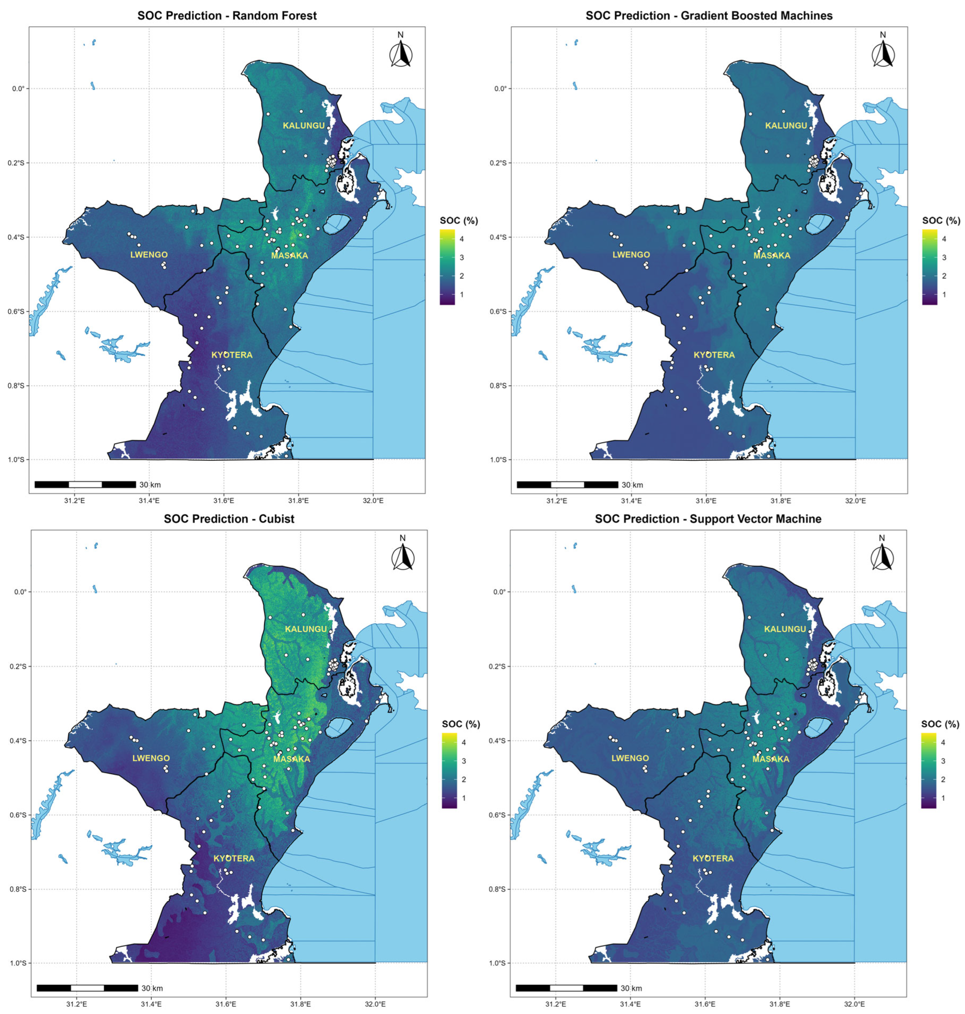
All four algorithms reproduced a broadly similar regional pattern, with relatively higher predicted SOCs in Kalungu and Central Masaka and lower values in Southern Kyotera and parts of Lwengo (Figure 2). The main difference among the models was the magnitude of local contrast rather than the location of the broad north–south pattern (Table 4).

Figure 2. Spatial distribution of SOC predicted by the four ML algorithms across the Robusta coffee-growing landscape. The white dots represent soil sampling locations.

Table 4. Descriptive statistics of wall-to-wall SOC predictions generated by the four models.

Model	Min. SOC (%)	Max. SOC (%)	Mean SOC (%)	Standard Deviation
Cubist	0.45	4.50	1.93	0.68
RF	0.69	4.11	1.79	0.43
SVM	1.15	2.74	1.78	0.31
GBM	1.30	2.56	1.77	0.26

Cubist produced the widest prediction range (0.45–4.50%; SD = 0.68), followed by RF (0.69–4.11%; SD = 0.43). SVM (1.15–2.74%; SD = 0.31) and GBM (1.30–2.56%; SD = 0.26) generated smoother surfaces concentrated more strongly around intermediate SOC values. Landscape mean predictions were comparatively similar for RF, SVM, and GBM (1.77–1.79%), while Cubist produced a higher mean of 1.93%.

3.5. Environmental Predictors Associated with SOC

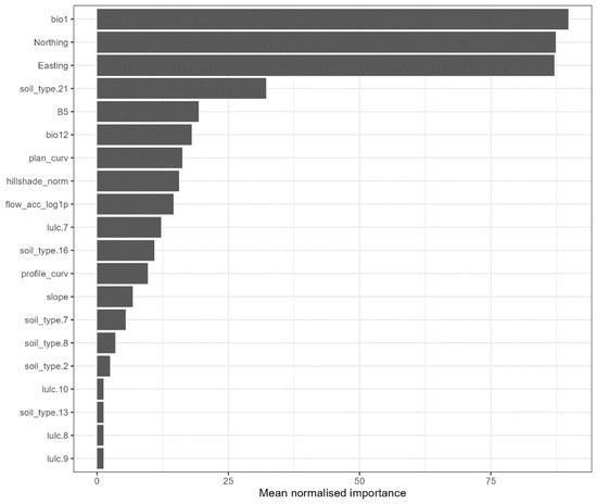
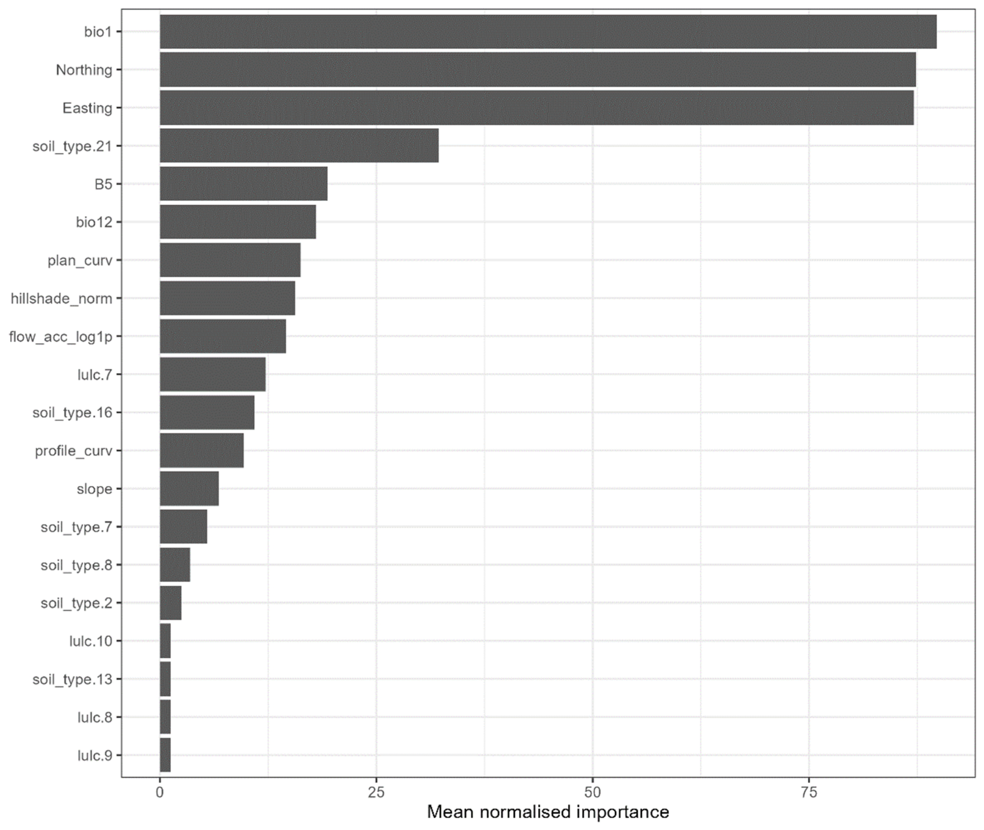
The descriptive cross-model variable-importance summary identified annual mean temperature (BIO1), Northing, and Easting as the highest-ranked predictors (Figure 3). A mapped soil class (soil_type.21), Landsat 9 Band 5, and annual precipitation (BIO12) formed the next group of influential predictors, while terrain and broad land-cover variables generally ranked lower. The prominence of Northing and Easting indicates a strong geographical trend in the fitted relationships, but these coordinates should be interpreted as spatial proxies for unmeasured or incompletely represented processes rather than as direct environmental controls on SOC.

Figure 3. Mean normalised variable importance across the machine-learning models.

The model-specific rankings were not identical. SVM emphasised annual mean temperature and spatial position, RF ranked Easting, temperature, and Northing highly, and GBM gave greatest importance to Northing, Easting, and temperature. The Cubist variable-importance output did not yield an interpretable model-specific bar pattern in the available diagnostic figure. Consequently, the normalised cross-model ranking is used as a descriptive synthesis and not as evidence that the four algorithms measure variable importance on an equivalent statistical scale.

3.6. Between-Model Prediction Disagreement

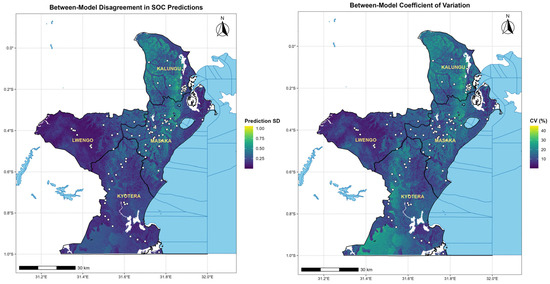
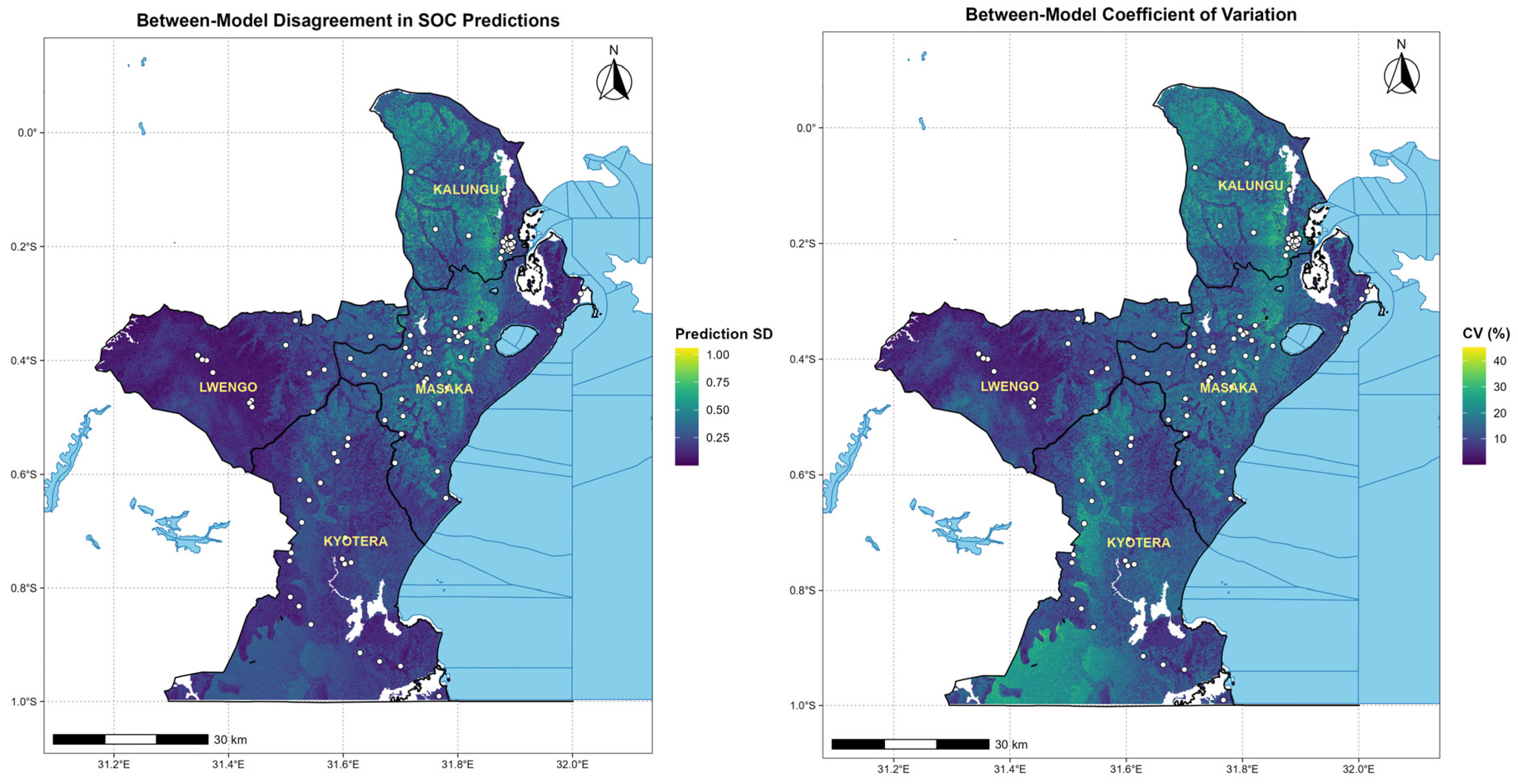
Between-model disagreement varied spatially across the study area (Figure 4). Cell-wise standard deviation and CV were relatively low across much of Lwengo and large parts of Kyotera, but higher local disagreement occurred in parts of Kalungu, Central Masaka, Southern Kyotera, and selected transition zones. These locations generally corresponded to areas where Cubist or RF predicted stronger local contrasts than the smoother SVM and GBM surfaces.

Figure 4. Spatial distribution of between-model disagreement in soil organic carbon (SOC) predictions from the four machine-learning models, expressed as the standard deviation of model predictions and the coefficient of variation (CV, %). White dots represent soil sampling locations.

The disagreement maps should be interpreted as sensitivity to algorithm choice rather than total SOC prediction uncertainty. High disagreement identifies areas where the mapped value is more model-dependent and where additional field observations may be particularly useful. Low disagreement indicates convergence among algorithms but does not, by itself, establish high predictive accuracy.

4. Discussion

4.1. Variability of SOC in the South–Central Uganda Coffee Landscape

Measured SOC varied from 0.31% to 5.30% and had a coefficient of variation of 62.7%, confirming substantial heterogeneity within the sampled coffee landscape. Such variability is plausible in smallholder Robusta systems where shade-tree structure, crop mixtures, residue management, manure use, soil disturbance, erosion exposure, and soil properties change markedly over short distances [7,10,11,12,13,21]. The observed positive skew indicates that low-to-moderate SOC values were common, while fewer locations had comparatively high SOC.

The field survey did not provide spatially complete management covariates, so the causes of high or low SOC at individual locations cannot be attributed confidently to particular farming practices. Manure application, mulching, coffee age, shade-tree density, tillage, residue retention, and previous land use are plausible mechanisms, but they remain unmeasured explanatory factors in this DSM. The measured SOC pattern should, therefore, be interpreted as the combined outcome of environmental, spatial, and management heterogeneity rather than as evidence for a single dominant control.

4.2. Comparative Performance of the Machine-Learning Models

SVM achieved the highest holdout R² and lowest RMSE, while Cubist produced the lowest MAE, smallest bias, and highest concordance. The ranking SVM > Cubist > RF > GBM is, therefore, consistent with Table 3, but the differences should be interpreted in the context of generally limited performance. The best model explained only 36% of the variance in the 24-point holdout. SVM has performed well in other East African SOC applications [25], while RF and mixed approaches have produced stronger results in studies with different sample sizes, environmental settings, and predictor sets [26,27]. These comparisons underline that algorithm performance is data- and landscape-dependent, rather than universally transferable.

Several factors likely contributed to the limited accuracy. First, 126 observations are sparse relative to a 4356-km² heterogeneous agricultural landscape, and the 24-point independent holdout provides an imprecise basis for estimating generalisation performance. Second, sample density was uneven across the study area. Third, farm-management variables that can strongly affect SOC were not available as spatial predictors. Fourth, the covariates differed in spatial and temporal support: field measurements were point observations from 2024, WorldClim represented long-term climate normals, land cover represented 2017, and Landsat imagery was acquired in 2025. Finally, the random holdout did not enforce geographic separation between the training and testing points. These limitations can weaken observed SOC–environment relationships and may also cause random-holdout metrics to differ from performance at geographically independent locations.

4.3. Spatial Distribution of Predicted SOC

The four algorithms agreed on a broad geographical pattern of higher SOC in Kalungu and Central Masaka and lower SOC in Southern Kyotera and parts of Lwengo but differed in the magnitude of local variation. Cubist and RF preserved a wider range of predictions, whereas SVM and GBM showed stronger shrinkage toward intermediate values. Agreement in a broad pattern is useful for landscape screening, but local differences among models show why individual pixel values should not be treated as equally reliable.

Annual mean temperature and spatial position were the highest-ranked predictors. Climate can influence SOC through vegetation productivity, soil moisture, microbial activity, and decomposition [2,3,4], but the importance of Easting and Northing requires particular caution. Coordinates do not directly represent soil-forming mechanisms. Rather, they can absorb the broad geographical structure associated with unmeasured management histories, soil gradients, landscape transitions, or other geographically structured processes. Their strong importance, therefore, supports the presence of a spatial trend within this study area but does not establish a causal effect of location itself, and it may reduce the transferability of the fitted relationships beyond the mapped landscape.

Mapped soil class, Landsat 9 Band 5, and annual precipitation provided additional predictive information. Soil classes can integrate broad differences in mineralogy, texture, drainage, and parent material, while Band 5 provides a spectral proxy related to vegetation structure. However, the 2025 Landsat acquisition does not exactly coincide with the 2024 soil survey, and broad land-cover classes cannot distinguish farm-level management. The environmental controls identified by the models should, therefore, be described as predictive associations, not deterministic drivers of SOC.

4.4. Implications for Coffee-Landscape Management

The main value of the prediction surfaces is to support landscape-level screening. Areas repeatedly mapped as relatively low SOC can be prioritised for confirmatory sampling, extension attention, or more detailed assessment, while areas of high between-model disagreement can guide future sampling because their mapped values are more sensitive to algorithm choice. The maps may also help stratify future surveys and identify environmental combinations that are poorly represented by the current observation network.

Management responses should not be prescribed from the maps alone. Practices such as residue retention, mulching, organic amendments, appropriate shade-tree management, cover crops, reduced disturbance, and erosion control may support soil-carbon maintenance, but their suitability depends on site-specific soil, slope, crop condition, farm resources, and management history. Plot-level soil testing and field assessment are still necessary before making farm-specific recommendations.

4.5. Study Limitations

The principal limitations are the modest sample size, uneven spatial distribution of observations, and the small independent holdout of 24 samples. Sampling was field-based rather than a regular spatial probability design, with greater observation density in Central Masaka and the Masaka–Kalungu area than in western Lwengo and Southern Kyotera. The predictions are consequently better supported for environmental and geographical conditions represented by the sample than in sparsely observed areas.

A second limitation is incomplete representation of farm management and temporal dynamics. Manure use, mulching, coffee age, shade-tree composition and density, tillage, residue management, and land-use history were not available as wall-to-wall predictors. In addition, the covariates originated from different periods and spatial resolutions. Resampling all layers to a 30 m grid ensured spatial alignment but did not increase the intrinsic information content of coarser climate or legacy mapping products. The between-model SD and CV further represent only disagreement among algorithms, not total predictive uncertainty.

The validation framework also has spatial limitations. The random holdout and internal five-fold cross-validation did not enforce geographic independence, and residual spatial autocorrelation has not been formally quantified. These issues should be addressed in additional analysis, where feasible. Future work should increase the number and spatial balance of observations, incorporate directly measured and spatially explicit farm-management variables, evaluate residual spatial dependence, and compare alternative validation designs before using the maps for more spatially demanding applications.

5. Conclusions

This study developed landscape-scale SOC predictions for a heterogeneous smallholder Robusta coffee area in South–Central Uganda using 126 field observations and four ML algorithms. Measured SOC was highly variable, and all four models reproduced a broad geographical pattern, though they differed substantially in local contrast.

Independent holdout performance was limited and ranked SVM > Cubist > RF > GBM. SVM achieved the highest R² (0.36) and lowest RMSE, while Cubist showed the lowest MAE, smallest bias, and highest concordance. These results do not support farm-scale precision prediction. Instead, they indicate that the maps are best used as screening tools to prioritise field verification and future sampling.

Annual mean temperature and spatial position were the highest-ranked predictors, followed by mapped soil type, Landsat 9 Band 5, and annual precipitation. The importance of Northing and Easting should be interpreted as evidence of residual geographical structure rather than a direct soil-forming effect. Likewise, associations with climate, soil, and spectral covariates should not be interpreted causally because important farm-management variables were not available as spatial predictors.

Between-model standard deviation and coefficient of variation identified locations where SOC predictions were more sensitive to algorithm choice; these measures represent model disagreement rather than total predictive uncertainty. Areas of high disagreement and sparsely sampled parts of Western Lwengo and Southern Kyotera are priority locations for additional observations.

Subsequent studies should improve spatial balance and sample size, incorporate farm-management and land-use history variables, and evaluate residual spatial autocorrelation and geographic independence in validation. Until then, the maps should complement—not replace—field-based soil assessment and should be applied primarily at the landscape-planning scale.

References

- Kitchen, N.R.; Clay, S.A. Understanding and identifying variability. In Precision Agriculture Basics; Wiley: Hoboken, NJ, USA, 2018; pp. 13–24. [Google Scholar] [CrossRef] [Scilit]
- McBratney, A.B.; Mendonça Santos, M.L.; Minasny, B. On digital soil mapping. Geoderma 2003, 117, 3–52. [Google Scholar] [CrossRef] [Scilit]
- Georgiou, K.; Jackson, R.B.; Vindušková, O.; Abramoff, R.Z.; Ahlström, A.; Feng, W.; Harden, J.W.; Pellegrini, A.F.A.; Polley, H.W.; Soong, J.L.; et al. Global stocks and capacity of mineral-associated soil organic carbon. Nat. Commun. 2022, 13, 3797. [Google Scholar] [CrossRef] [Scilit] [PubMed]
- Wadoux, A.M.J.C.; Saby, N.P.A.; Martin, M.P. Shapley values reveal the drivers of soil organic carbon stock prediction. SOIL 2023, 9, 21–38. [Google Scholar] [CrossRef] [Scilit]
- Tully, K.; Sullivan, C.; Weil, R.; Sanchez, P. The State of soil degradation in sub-Saharan Africa: Baselines, trajectories, and solutions. Sustainability 2015, 7, 6523–6552. [Google Scholar] [CrossRef] [Scilit]
- Lal, R. Restoring soil quality to mitigate soil degradation. Sustainability 2015, 7, 5875–5895. [Google Scholar] [CrossRef] [Scilit]
- Kyalo, G.; Apunyo, P.C.; Mwanjalolo, M.; Luswata, C.K.; Kawooya, R.; Niyibigira, E.I. Characterisation and Mapping of Soils in Major Coffee Growing Regions of Uganda. J. Agric. Sci. 2023, 16, 49. [Google Scholar] [CrossRef] [Scilit]
- Minai, O. Assessing the Spatial Variability of Soils in Uganda Part of the African Languages and Societies Commons, and the Agriculture Commons Recommended Citation. 2015. Available online: https://docs.lib.purdue.edu/open_access_theses/581 (accessed on 12 July 2026).
- Wang, N.; Jassogne, L.; van Asten, P.J.A.; Mukasa, D.; Wanyama, I.; Kagezi, G.; Giller, K. Evaluating coffee yield gaps and important biotic, abiotic, and management factors limiting coffee production in Uganda. Eur. J. Agron. 2015, 63, 1–11. [Google Scholar] [CrossRef] [Scilit]
- Nakyagaba, W.N.; Talwana, H.; Kyamanywa, S.; Kagezi, G.H.; Bamutaze, Y.; Mfitumukiza, D.; Twinomuhangi, R.; Bukomeko, H.; Mukasa, D.; Fungo, B.; et al. Biophysical Constraints to Robusta Coffee Productivity in Low, Moderate, and High Rainfall Areas. Int. J. Agron. 2024, 2024, 4683226. [Google Scholar] [CrossRef] [Scilit]
- Apanovich, N.; Lenssen, A.W. Cropping systems and soil quality and fertility in south-central Uganda. Afr. J. Agric. Res. 2018, 13, 792–802. [Google Scholar] [CrossRef] [Scilit][Green Version]
- Mulinde, C.; Majaliwa, J.G.M.; Twinomuhangi, R.; Mfitumukiza, D.; Waiswa, D.; Tumwine, F.; Kato, E.; Asiimwe, J.; Nakyagaba, W.N.; Mukasa, D. Projected climate in coffee-based farming systems: Implications for crop suitability in Uganda. Reg. Environ. Change 2022, 22, 83. [Google Scholar] [CrossRef] [Scilit]
- Bongers, G.; Fleskens, L.; Van De Ven, G.; Mukasa, D.; Giller, K.; Van Asten, P. Diversity in Smallholder Farms Growing Coffee and their use of Recommended Coffee Management Practices in Uganda. Exp. Agric. 2015, 51, 594–614. [Google Scholar] [CrossRef] [Scilit]
- Hengl, T.; Leenaars, J.G.B.; Shepherd, K.D.; Walsh, M.G.; Heuvelink, G.B.M.; Mamo, T.; Tilahun, H.; Berkhout, E.; Cooper, M.; Fegraus, E.; et al. Soil nutrient maps of Sub-Saharan Africa: Assessment of soil nutrient content at 250 m spatial resolution using machine learning. Nutr. Cycl. Agroecosyst. 2017, 109, 77–102. [Google Scholar] [CrossRef] [Scilit] [PubMed]
- Poggio, L.; de Sousa, L.M.; Batjes, N.H.; Heuvelink, G.B.M.; Kempen, B.; Ribeiro, E.; Rossiter, D. SoilGrids 2.0: Producing soil information for the globe with quantified spatial uncertainty. SOIL 2021, 7, 217–240. [Google Scholar] [CrossRef] [Scilit]
- Padarian, J.; Minasny, B.; McBratney, A.B. Using deep learning for digital soil mapping. SOIL 2019, 5, 79–89. [Google Scholar] [CrossRef] [Scilit]
- Minasny, B.; Bandai, T.; Ghezzehei, T.A.; Huang, Y.C.; Ma, Y.; McBratney, A.B.; Ng, W.; Norouzi, S.; Padarian, J.; Rudiyanto; et al. Soil Science-Informed Machine Learning. Geoderma 2024, 452, 117094. [Google Scholar] [CrossRef] [Scilit]
- Breiman, L. Random Forests. Mach. Learn. 2001, 45, 5–32. [Google Scholar] [CrossRef] [Scilit]
- Friedman, J.H. Greedy Function Approximation: A Gradient Boosting Machine. Ann. Stat. 2001, 29, 1189–1232. [Google Scholar] [CrossRef] [Scilit]
- Kuhn, M.; Johnson, K. Applied Predictive Modeling; Springer: New York, NY, USA, 2013. [Google Scholar] [CrossRef] [Scilit]
- Tumwebaze, S.B.; Byakagaba, P. Soil organic carbon stocks under coffee agroforestry systems and coffee monoculture in Uganda. Agric. Ecosyst. Environ. 2016, 216, 188–193. [Google Scholar] [CrossRef] [Scilit]
- Nsubuga, F.W.; Mukarugwiza, O.J.; Rautenbach, C.J.D. Variability properties of daily and monthly observed near-surface temperatures in Uganda: 1960–2008. Int. J. Climatol. 2014, 34, 303–314. [Google Scholar] [CrossRef] [Scilit]
- Okalebo, R.; Gathua, K.W.; Woomer, P.L. Laboratory Methods of Soil and Plant Analysis: A Working Manual, 2nd ed.; The Sustainable Agriculture Centre for Research Extension and Development in Africa: Nairobi, Kenya, 2002. [Google Scholar]
- Fick, S.E.; Hijmans, R.J. WorldClim 2: New 1-km spatial resolution climate surfaces for global land areas. Int. J. Climatol. 2017, 37, 4302–4315. [Google Scholar] [CrossRef] [Scilit]
- Were, K.; Bui, D.T.; Dick, Ø.B.; Singh, B.R. A comparative assessment of support vector regression, artificial neural networks, and random forests for predicting and mapping soil organic carbon stocks across an Afromontane landscape. Ecol. Indic. 2015, 52, 394–403. [Google Scholar] [CrossRef] [Scilit]
- Tobore, A.O.; Nkwunonwo, U.C.; Abdussalaam, S.A.; Oyerinde, G.; Samson, V.M.; Adeoba, A.Q.; Adedeji, H.O.; Odebode, A.M.; Adelana, A.O. Random forest algorithm and remote sensing techniques for wetland soil organic carbon prediction towards environmental sustainability. Discov. Environ. 2025, 3, 222. [Google Scholar] [CrossRef] [Scilit]
- Silatsa, F.B.T.; Yemefack, M.; Tabi, F.O.; Heuvelink, G.B.M.; Leenaars, J.G.B. Assessing countrywide soil organic carbon stock using hybrid machine learning modelling and legacy soil data in Cameroon. Geoderma 2020, 367, 114260. [Google Scholar] [CrossRef] [Scilit]
Disclaimer/Publisher’s Note: The statements, opinions and data contained in all publications are solely those of the individual author(s) and contributor(s) and not of MDPI and/or the editor(s). MDPI and/or the editor(s) disclaim responsibility for any injury to people or property resulting from any ideas, methods, instructions or products referred to in the content. |
© 2026 by the authors. Licensee MDPI, Basel, Switzerland. This article is an open access article distributed under the terms and conditions of the Creative Commons Attribution (CC BY) license.