


Abstract
Arid mountain–oasis–desert regions exhibit strong terrain and surface-cover heterogeneity that is difficult to represent using conventional land-cover classification schemes. This study developed an ecosystem-oriented hierarchical framework for the Kashi region by combining a terrain-constrained Mountain extraction method with Automatic Deep Forest Shrinkage model (ADeFS). Nine ecosystem elements were defined: Mountain, Water, Forest, Cropland, Lake, Grassland, Desert, Ice, and Human. Mountain was first delineated as an independent physiographic element using a locally derived baseline surface, relative relief, slope, and topographic position, thereby reducing semantic overlap between terrain units and spectrally similar surface-cover classes. ADeFS was then adapted to classify the seven non-mountain classes, and Lake was subsequently separated from the unified Water class through visual interpretation. The results show that ADeFS achieved the highest accuracy, with an overall accuracy of 88.7% and a Kappa coefficient of 0.868. Independent field validation of the 2026 map yielded an overall accuracy of 86.2% and a Kappa coefficient of 0.825. From 2015 to 2026, the mountain-oasis-desert structure remained broadly stable, while Desert and Ice decreased and Forest, Grassland, and Cropland expanded. Ecosystem-element transitions were concentrated before 2021 and weakened thereafter. Landscape metrics showed that Desert remained the dominant matrix, Grassland had the highest patch density and edge density, and Cropland became increasingly aggregated within oasis agricultural areas. The framework provides an ecologically interpretable approach for ecosystem-element mapping and long-term monitoring in arid heterogeneous regions.
1. Introduction
Since the mid-twentieth century, rapid population growth, urbanization, and intensified land use have exerted increasing pressure on natural ecosystems, resulting in habitat loss, landscape fragmentation, biodiversity decline, and the degradation of ecosystem functions [1,2]. These widespread ecological changes have posed substantial challenges to biodiversity conservation, ecosystem stability, and global sustainable development. In response to the continuing degradation of ecosystems worldwide, the United Nations General Assembly proclaimed 2021–2030 as the United Nations Decade on Ecosystem Restoration, calling for coordinated global action to prevent, halt, and reverse ecosystem degradation [3].
China has implemented many large-scale ecological conservation and restoration programs since the late twentieth century, including the Three-North Shelterbelt Program [4], the Natural Forest Conservation Program [5], the Grain for Green Program [6], and national wetland and grassland restoration initiatives [7]. These programs have contributed substantially to vegetation recovery, ecosystem conservation, and the improvement of regional ecological conditions [7,8]. Alongside these restoration practices, China has increasingly shifted from the management of individual ecological components toward integrated ecosystem conservation and restoration. This transition is embodied in the concept that mountains, rivers, forests, farmlands, lakes, grasslands, and deserts form a community of life, which emphasizes the interdependence of natural elements and the need to coordinate ecological processes across entire landscapes [9]. Under this systems-oriented perspective, accurately identifying ecosystem elements and characterizing their spatial organization have become fundamental requirements for ecological monitoring, integrated environmental management, and sustainable regional development.
Against this background, arid and semi-arid regions have received increasing attention because their ecosystems are generally characterized by limited water availability, low environmental resilience, and are particularly vulnerable to the joint impacts of climate change and human disturbance [10]. The Kashi region is a representative arid landscape composed of mountains, alluvial plains, oases, grasslands, deserts, and inland water bodies [11]. Pronounced topographic and hydrological gradients create strong spatial heterogeneity, while agricultural expansion, urban development, and changing water availability further reshape the regional landscape. The close spatial coupling of natural and human-dominated ecosystem elements makes Kashi a suitable region for investigating ecosystem-oriented classification and the spatiotemporal dynamics of complex mountain–oasis–desert systems.
Remote-sensing observations now support land-use and land-cover mapping over a wide range of spatial extents, from individual landscapes to regional and global domains. Previous studies have employed multi-temporal and multi-sensor satellite observations to characterize regional land-cover patterns and changes, while index-based extraction and machine-learning algorithms have been applied to identify major classes such as cropland, built-up land, desert surfaces, and water bodies [12,13]. These approaches have substantially improved the efficiency and accuracy of thematic land-cover mapping in arid environments. However, conventional LULC frameworks generally represent the landscape as a set of discrete and mutually exclusive surface categories, with classification primarily determined by spectral or structural similarity. Although suitable for inventories of individual land-cover types, such frameworks provide only limited representation of the abiotic setting, ecological processes, and spatial interdependence that collectively define ecosystem organization. Ecosystem-level characterization, in contrast, requires the integration of biotic components, abiotic environments, ecological functions, and their spatial relationships within a coherent and hierarchical framework [14]. Therefore, moving beyond isolated land-cover classes toward an ecosystem-oriented classification system is necessary for representing the structural complexity and ecological connectivity of heterogeneous mountain–oasis–desert landscapes.
These limitations are particularly pronounced in arid heterogeneous regions such as Kashi, where steep topographic gradients, strong hydro-climatic constraints, and highly interwoven mountain, oasis, desert, vegetation, and human-dominated land create substantial spectral and spatial heterogeneity [10]. Complex terrain further alters illumination conditions, surface scattering, as well as the spatial arrangement of land-cover classes, thereby increasing confusion among classes with similar spectral or structural characteristics [15]. Recent advances in machine learning and deep representation learning have improved the capacity to model nonlinear relationships and extract discriminative features from remote sensing observations. At the same time, the integration of optical imagery, synthetic aperture radar data, and topographic variables provides complementary information on surface reflectance, vegetation structure, moisture conditions, roughness, and terrain configuration, offering clear advantages over single-source observations for heterogeneous landscape mapping [16]. Nevertheless, improved algorithms and richer input data alone do not fully address the semantic overlap and spatial coupling among ecosystem elements. Their effective use therefore requires an ecosystem-oriented and hierarchically organized classification framework that incorporates both multi-source observations and ecological prior knowledge.
Previous studies have explored hierarchical and terrain-assisted strategies to improve land-cover classification in arid and mountainous environments. Hierarchical object-oriented decision-tree approaches have been used to distinguish vegetation communities in arid rangelands [17], while terrain-related variables have been incorporated as auxiliary predictors in machine-learning classification of desert–oasis landscapes [18]. More recently, geographic subdivision combined with hierarchical decision-tree classification has also been applied to long-term land-cover mapping in complex mountain regions [19]. However, these approaches generally employ terrain information as auxiliary predictors, spatial subdivision criteria, or classification rules within conventional land-cover schemes. In contrast, the present study explicitly represents Mountain as a terrain-defined physiographic ecosystem element and separates its delineation from the classification of surface-cover ecosystem elements, thereby linking physiographic structure with ecosystem-element mapping and subsequent landscape-dynamics analysis.
Accordingly, this study develops an ecosystem-oriented hierarchical classification framework for the Kashi region by integrating multi-source remote sensing observations with ecological prior knowledge. Unlike conventional terrain-assisted land-cover classification, the proposed framework explicitly distinguishes Mountain as a terrain-defined physiographic ecosystem element from the subsequent classification of surface-cover ecosystem elements. A regionally adapted ecosystem-element scheme encompassing Mountain, Water, Forest, Cropland, Lake, Grassland, Desert, Ice, and Human-dominated land is first established. The terrain-derived Mountain layer is independently delineated, while the surface-cover ecosystem elements are classified using the Automatic Deep Forest Shrinkage model (ADeFS) with complementary optical, SAR, spectral-index, and topographic features. Finally, annual ecosystem-element maps from 2015 to 2026 are generated to evaluate classification performance and examine spatial patterns, land-cover transitions, and landscape dynamics. Through this framework, the study seeks to improve both the mapping accuracy and ecological interpretability of land classification in arid heterogeneous regions.
2. Materials and Methods
2.1. Study Area
The Kashi region (71°39′–79°52′ E, 35°28′–40°16′ N) is located in southwestern Xinjiang, China, along the western margin of the Tarim Basin (Figure 1). It is bounded by the Kunlun Mountains to the south, the southern branches of the Tianshan Mountains to the north, and the Pamir Plateau to the west. The southwestern part of the region extends into the Karakoram Mountains, where K2 lies along the China–Pakistan border. This high-mountain setting contributes to an exceptionally large elevation gradient across the study area, while the maximum elevation represented by the DEM used in this study is approximately 8564 m. Elevation generally decreases from the southwestern highlands toward the northeastern plains, forming a pronounced topographic gradient and a diverse landscape composed of high mountains, piedmont plains, river valleys, oases, grasslands, and extensive desert surfaces. This strong topographic contrast provides a clear physiographic basis for distinguishing Mountain as a terrain-defined ecosystem element. The region experiences a temperate continental arid climate with low precipitation, intense evaporation, abundant solar radiation, and large seasonal temperature variations. Within the Kashi Oasis, the mean annual temperature is approximately 11.8 °C, precipitation is about 71.4 mm yr−1, and potential evaporation approaches 2000 mm yr−1, reflecting the pronounced aridity of the regional environment [20]. Water availability and ecosystem development are strongly dependent on runoff supplied by mountain snow and glacier melt, together with river flow and groundwater. This strong dependence on limited and spatially uneven water resources makes the regional environment particularly sensitive to hydrological variability, desertification, and land degradation [13].
Figure 1.
Geographic location and elevation map of the study area: (a) location of Xinjiang in China; (b) location of Kashi in Xinjiang; (c) digital elevation model (DEM) and administrative divisions of Kashi.
The Kashi region is characterized by a highly heterogeneous mountain–oasis–desert landscape, in which cropland and human-dominated land are concentrated mainly in the oasis plains, while grassland, desert, water bodies, and snow and ice occur primarily in the surrounding piedmont and mountain areas. These landscape elements provide essential ecosystem services, including food production, water regulation, soil conservation, carbon storage, and habitat maintenance [21]. However, the continued expansion of cultivated and built-up land has reshaped regional landscape patterns and intensified ecological pressure in the oasis–desert transition zone [22]. The close coupling between natural gradients and human activities makes Kashi a representative region for ecosystem-oriented classification supported by remote-sensing data.
2.2. Data Collection
This study integrated optical, synthetic aperture radar (SAR), and topographic data to characterize the spectral, structural, and terrain-related properties of ecosystem elements. Harmonized Landsat and Sentinel-2 (HLS) surface reflectance data provided multispectral observations at 30 m spatial resolution, Sentinel-1 SAR data supplied complementary information on surface scattering and vegetation structure, and the Shuttle Radar Topography Mission (SRTM) digital elevation model was used to derive terrain variables. Dataset-specific preprocessing was performed according to the characteristics of each source, including quality masking and temporal compositing for HLS, radiometric calibration, speckle filtering, and terrain correction for Sentinel-1, and projection and grid alignment for the topographic and reference datasets. All datasets were ultimately resampled and co-registered to a common 30 m spatial grid to ensure spatial consistency. Data preprocessing was performed using Google Earth Engine (Google LLC, Mountain View, CA, USA) and ArcGIS Pro 3.0.0 (Esri, Redlands, CA, USA). The principal datasets and their roles in this study are summarized in Table 1.
Four land-cover products, including GLC_FCS30, CLCD, ESA WorldCover, and MODIS Land Cover, were integrated to generate reliable annual reference samples for the six years from 2015 to 2020, as shown in Figure 2a–f. Reference-sample construction was limited to this period because comparable multi-source annual land-cover products were not consistently available for the subsequent years. Their original classification systems were first harmonized to the ecosystem-element scheme and spatially aligned to a common 30 m grid. A weighted voting method was then applied to identify high-confidence pixels with consistent labels across products, with weights assigned according to the reported thematic accuracy and spatial resolution of each dataset. This multi-product fusion reduces product-specific uncertainty and improves the robustness of the resulting reference samples [23].
Figure 2.
Spatial distribution of the sample datasets used in this study. Panels (a–f) show the reference samples derived from the weighted-voting maps for 2015–2020, and panel (g) shows the independent field samples collected in 2026, overlaid on the HLS true-color imagery.
Table 1.
Multi-source datasets used for ecosystem-element classification.
An independent field survey was conducted across the Kashi region from 30 June to 5 July 2026, to validate the final classification map. A total of 239 georeferenced samples were collected for six ecosystem-element classes: cropland, forest, grassland, water, desert, and human-dominated land; the spatial distribution of the independent field-validation samples is shown in Figure 2g. The location and class label of each sample were recorded in situ and matched to the corresponding pixel in the 2026 ecosystem-element map. These samples were retained only for independent accuracy evaluation and were not used during model training, feature selection, and parameter optimization, thereby ensuring that the validation results reflected the generalization performance of the final map [31].
3. Ecosystem-Oriented Classification Methodology
The proposed methodology consists of four main stages, as illustrated in Figure 3. First, multi-source datasets were collected and preprocessed to construct classification features and reference samples. Second, a regionally adapted ecosystem-element scheme was established to represent: (i) mountains, (ii) water, (iii) forests, (iv) croplands, (v) lakes, (vi) grasslands, (vii) desert, (viii) ice, and (ix) human-dominated lands. Third, two complementary classification components were implemented independently: Mountain was delineated as a terrain-defined physiographic ecosystem element using topographic constraints, while the surface-cover ecosystem elements were classified using ADeFS. Finally, classification outcomes were assessed using the reference dataset together with independent field observations, and the annual maps from 2015 to 2026 were further analyzed to characterize spatial patterns, land-cover transitions, and landscape dynamics.
Figure 3.
Overall workflow of the ecosystem-oriented hierarchical classification methodology in this study.
3.1. Ecosystem-Element Classification Scheme
Conventional land-use and land-cover classification systems primarily distinguish surface types according to their observable spectral, structural, or functional characteristics. Although these systems are effective for thematic mapping, they provide only limited representation of the abiotic settings, ecological processes, and spatial relationships that collectively organize regional ecosystems [9,32]. To address this limitation, this study introduces an ecosystem-element classification scheme inspired by the integrated life-community concept of mountains, rivers, forests, farmlands, lakes, grasslands, and deserts, which emphasizes the interdependence and coordinated functioning of different ecological components [7,33]. Considering the environmental characteristics and remote-sensing separability of the Kashi region, nine ecosystem elements were defined: Mountain, Water, Forest, Cropland, Lake, Grassland, Desert, Ice, and Human-dominated land.
Because the nine ecosystem elements represent different ecological dimensions, including terrain, land cover, hydrology, cryosphere, and human influence, a hierarchical strategy was adopted to reduce semantic overlap among classes. Mountain areas were first delineated using topographic constraints, after which the non-mountain areas were classified according to their vegetation, water, ice, desert-surface, and anthropogenic characteristics. Within the unified water class, standing water bodies were subsequently identified as lakes through visual interpretation, whereas flowing and channelized water bodies remained classified as water. Human-dominated land encompassed settlements, industrial and commercial areas, transportation infrastructure, and other artificial surfaces. The resulting regionally adapted classification scheme is summarized in Table 2.
Table 2.
Ecosystem-element classification scheme and class definitions.
3.2. Multi-Source Feature Construction
To characterize the spectral, structural, and topographic differences among ecosystem elements, a multi-source feature set was constructed from HLS surface reflectance, Sentinel-1 SAR data, and DEM-derived terrain variables. Features were selected according to the environmental characteristics of the Kashi mountain–oasis–desert system and their expected contribution to class separability, rather than by directly stacking all available variables. The HLS multispectral bands provided harmonized surface-reflectance information across the visible, near-infrared, and shortwave-infrared regions, enabling the characterization of vegetation condition, surface moisture, exposed substrates, ice, and artificial surfaces [34].
Sentinel-1 VV (vertical transmit–vertical receive) and VH (vertical transmit–horizontal receive) backscatter coefficients were used to characterize differences in surface scattering, dielectric properties, and vegetation structure. The VV/VH ratio was included to enhance polarization contrast among vegetation, water, desert surfaces, and human-dominated land, while the Radar Vegetation Index (RVI) was calculated to represent vegetation-related volume scattering and canopy structural variation. These complementary SAR features provided structural and moisture-sensitive information that was not fully captured by optical reflectance alone.
DEM-derived variables were used for two distinct purposes. Relative relief, slope, and topographic position were employed in the terrain-constrained extraction of Mountain areas, whereas local terrain roughness was retained as the topographic input for ADeFS classification of the non-mountain ecosystem elements. This separation avoided introducing redundant terrain variables into the classification model while preserving the topographic information needed to distinguish heterogeneous surfaces. All classification features were spatially aligned and resampled to a common 30 m grid before model training. The final feature set and its primary roles are summarized in Table 3.
Table 3.
Multi-source features used for ADeFS-based ecosystem-element classification.
3.3. Hierarchical Ecosystem Classification Framework
To incorporate ecological prior knowledge and reduce semantic overlap between physiographic units and surface-cover classes, a terrain-constrained hierarchical classification strategy was developed. The procedure consisted of two sequential stages. First, Mountain areas were delineated from DEM-derived terrain variables as an independent physiographic element. The remaining non-mountain areas were then classified using ADeFS with the constructed optical, spectral-index, SAR, and terrain-roughness features. This hierarchical design separates terrain-defined Mountain from surface-cover elements and improves the ecological consistency and interpretability of the final ecosystem-element map.
3.3.1. Terrain-Based Mountain Extraction
Mountain was treated as a terrain-defined physiographic element rather than a conventional land-cover class and was therefore delineated before the classification of the remaining ecosystem elements. This terrain-derived Mountain layer was not used as a training label for ADeFS. Mountain extraction was based on the 30 m SRTM DEM, which provides spatially continuous elevation information for regional terrain analysis [26]. A terrain-constrained approach combining relative relief, slope, and topographic position was adopted because these variables jointly characterize vertical differentiation, terrain steepness, and the local position of landforms within their surrounding landscape [42]. The DEM was subsequently used to derive the local baseline surface, relative relief, slope, and topographic position required for Mountain extraction.
Specifically, a local baseline surface was first constructed to quantify the relative elevation of each pixel with respect to its surrounding low-lying terrain. For a target pixel , the baseline elevation was defined as the 10th percentile of elevations within a circular neighborhood with a radius of approximately 2 km
where denotes the DEM elevation. Based on this local baseline, the relative relief was calculated as
which measures the elevation difference between the target pixel and its surrounding terrain. In addition, the topographic position index (TPI) was used to indicate whether a pixel is locally higher than its neighborhood
where is the mean elevation within a local neighborhood . Slope was derived directly from the DEM using the standard terrain function.
A rule-based decision model was then used to identify mountain pixels. Relative relief was taken as the primary criterion, while slope and TPI were used as auxiliary constraints. A pixel was classified as mountain when its relative relief was at least 200 m and either its slope was no less than 5° or its TPI was positive
where = 200 m and = 5°. This rule emphasizes terrain with pronounced relative elevation differences while retaining locally elevated ridge and upper-slope positions. To improve spatial coherence, the initial mountain mask was refined by morphological opening with a 60 m circular kernel, followed by connected-component filtering to remove isolated patches smaller than 0.5 ha. Let denote the size of the connected component containing pixel , and let denote the minimum number of pixels corresponding to the minimum mapping unit. The final mountain mask can be expressed as
where is the morphologically refined mask. The resulting binary mountain mask was ultimately integrated with the ADeFS-derived classification results as an independent physiographic class, thereby forming the final ecosystem-element classification system. The original thresholds of 200 m for relative relief and 5° for slope were used as the baseline configuration for Mountain delineation. To assess parameter sensitivity, relative-relief thresholds of 150, 200, and 250 m and slope thresholds of 3°, 5°, and 7° were tested. All other parameters were kept unchanged.
3.3.2. ADeFS-Based Classification of Non-Mountain Ecosystem Elements
Following the establishment of the ecosystem-element scheme, multi-source feature construction, and terrain-based mountain extraction, the remaining non-mountain areas were classified into seven surface-cover classes: forest, cropland, grassland, water, desert, ice, and human-dominated lands. Lake was initially included in the unified Water class and was subsequently delineated through visual interpretation. For this purpose, the ADeFS model was adapted to multi-class ecosystem-element classification. ADeFS extends the multi-Grained Cascade Forest architecture by introducing LASSO- and Elastic-Net-based shrinkage to identify and retain the most informative forest components, thereby reducing model redundancy and computational cost while preserving the multilayer representation capability of deep forest [43]. The cascade structure progressively transforms the input features and learns nonlinear class representations through layer-wise forest ensembles. Compared with deep neural networks, gcForest generally requires less hyperparameter tuning, adaptively determines its model depth according to validation performance, and can perform effectively with relatively limited training samples [44]. These characteristics make the adapted ADeFS model suitable for multi-source ecosystem-element classification, where heterogeneous features and limited labeled samples are common challenges. By eliminating redundant forests and suppressing low-contribution components, ADeFS balances classification performance and computational efficiency. The adapted framework comprises four main components: multi-grained scanning, cascade forest learning, forest-level shrinkage, and ensemble classification, as illustrated in Figure 4.
Figure 4.
Architecture of the adapted Automatic Deep Forest Shrinkage model (ADeFS).
- (i)
- Multi-Grained Scanning: This module is designed to capture diverse local patterns within the input feature space. A seed-controlled random window strategy is employed to generate multiple local views of the original feature set. Specifically, the starting position of each window is randomly determined while the window size and number of windows remain fixed, thereby producing heterogeneous feature subsets and enhancing feature diversity. Each resulting feature is subsequently fed into both a Random Forest (RF) and a Completely Random Forest (CRF). The class-probability outputs produced by all forests are concatenated to form an enriched representation, which is then used as the input to the subsequent cascade structure. By integrating complementary local feature responses from different window positions and forest types, the MGS module strengthens the representation of the spectral, structural, and topographic heterogeneity among ecosystem elements.
- (ii)
- Cascade Forest: The cascade forest module performs hierarchical representation learning through a layer-by-layer ensemble structure. At each cascade layer, multiple Random Forests (RFs) and Completely Random Forests (CRFs) are used as base learners. Each RF or CRF contains an ensemble of decision trees whose probability estimates are aggregated to form the output representation of that forest. The outputs of all forests within the same layer are then concatenated to form an enhanced feature representation. At the n-th cascade layer, the input is obtained by combining the feature representation from the preceding layer with its forest outputs
- (iii)
- Elastic-Net-Based Forest Shrinkage: After the optimal cascade depth is determined, the class-probability outputs of all forests in the final cascade layer are concatenated and used as inputs to an Elastic-Net-regularized multinomial logistic regression model. Its objective function can be expressed as
For each forest, its class-specific coefficient block is extracted, and the corresponding norm is calculated as the forest importance score. According to the implemented strategy, forests with scores equal to or above the median are retained, corresponding approximately to the most influential 50% of the final-layer forests. This forest-level shrinkage reduces structural redundancy and computational burden while preserving the learners with stronger discriminative contributions.
- (iv)
- Coefficient-Weighted Ensemble Classification: The forests retained after the shrinkage step were integrated using a coefficient-weighted ensemble strategy. The importance scores derived from the Elastic Net coefficient blocks were normalized and used as ensemble weights to combine the class-probability outputs of the selected forests. Forests with stronger discriminative contributions were therefore assigned greater influence in the final prediction. The aggregated probabilities were subsequently normalized, with the highest-probability category taken as the final prediction.
Compared with the simple-average ensemble used in the original framework, this improvement establishes a direct connection between forest selection and final prediction, thereby reducing the influence of weak learners and enhancing the robustness of the classification results. To evaluate the effectiveness of the proposed method, four widely used classification models, including Random Forest (RF), LightGBM, Support Vector Machine (SVM), and Multilayer Perceptron (MLP), were selected as benchmark models. All models were trained and evaluated using the same reference samples, input features, and training–validation partition to ensure a consistent and fair comparison.
3.4. Accuracy Assessment Metrics
To evaluate the classification performance of the adapted ADeFS model and ensure a fair comparison with the benchmark models, including RF, LightGBM, SVM, and MLP, a total of 9340 reference samples were randomly divided into training and validation subsets at a ratio of 7:3, resulting in 6538 training samples and 2802 validation samples. All models were trained and evaluated using the same samples, input features, and data partition. Model predictions for the validation subset were cross-tabulated against the reference labels to obtain a confusion matrix for each classifier, with reference categories arranged by row and predicted categories by column. Four complementary measures, namely Overall Accuracy (OA), Kappa, Producer’s Accuracy (PA), and User’s Accuracy (UA), were used to quantify overall agreement and class-level classification performance [31].
OA represents the proportion of all validation samples that were correctly classified and was calculated as
where C denotes the total number of land-cover categories, represents the correctly predicted samples for class i, and N refers to the full validation sample size. The Kappa coefficient was then used to quantify prediction–reference agreement while correcting for agreement expected by chance
where is the observed agreement, equivalent to OA, and is the expected agreement by chance, calculated as
where and denote the row and column totals for class i, respectively. PA for class i was calculated as
PA measures class-specific agreement from the reference-data perspective and is therefore associated with omission error:
UA represents the proportion of samples predicted as class i that actually belonged to that class and therefore reflects commission error.
For cross-model feature comparison, permutation importance was calculated on the same validation set using classification accuracy as the scoring metric, and the resulting positive importance scores were normalized within each model. In addition, pairwise continuity-corrected McNemar tests were conducted between ADeFS and each benchmark classifier to evaluate the statistical significance of performance differences, with p < 0.05 considered significant.
4. Results
4.1. Feature Importance and Model Interpretation
The five classification models were trained using 18 input features, comprising 10 HLS spectral bands, three spectral indices (NDVI, NDWI, and SAVI), four Sentinel-1 SAR features (VV, VH, VV/VH, and RVI), and one DEM-derived terrain feature (Roughness). To ensure comparability among models with different internal structures, feature importance was evaluated using a unified permutation-based approach on the same validation dataset. The resulting importance scores were normalized within each model to quantify the relative contribution of individual predictors to ecosystem-element discrimination (Figure 5).
Figure 5.
Relative importance of the 18 input features across ADeFS, RF, LightGBM, SVM, and MLP for ecosystem-element classification.
The permutation-importance analysis revealed both common feature dependencies and model-specific differences across the five classifiers. For ADeFS, NDVI and terrain Roughness remained the two most influential variables, contributing 19.1% each, followed by SAVI (15.5%), NDWI (11.5%), and B7 (9.6%). Together, these five variables accounted for approximately 74.8% of the total relative importance, indicating that vegetation condition, surface moisture, shortwave-infrared reflectance, and terrain heterogeneity provided the principal discriminatory information for ADeFS. Random Forest showed a particularly strong dependence on Roughness (approximately 42.5%) and SAVI (26.6%), whereas LightGBM assigned the highest importance to SAVI (approximately 28.5%) and Roughness (20.5%). SVM exhibited a more distributed importance pattern, with SAVI, B7, NDVI, and Roughness among its dominant predictors, while MLP relied comparatively strongly on B6, NDVI, B7, SAVI, and NDWI. Overall, although the relative rankings varied among model architectures, terrain Roughness, SAVI, B7, and other vegetation- and moisture-related variables consistently emerged as important predictors across multiple classifiers.
4.2. Comparative Performance of Classification Models
The classification performance of ADeFS was compared with four benchmark models, namely RF, LightGBM, SVM, and MLP. All models were trained using the same 18 input features and evaluated using the same validation dataset containing 2802 samples. OA and the Kappa coefficient were used to assess overall performance, while PA and UA were used to evaluate class-specific performance, with the overall comparison summarized in Table 4.
Table 4.
Overall classification performance of ADeFS and the benchmark models.
ADeFS achieved the highest overall performance, with an OA of 88.7% and a Kappa coefficient of 0.868 (Table 4). Compared with RF, LightGBM, SVM, and MLP, ADeFS improved OA by 2.1, 2.5, 1.7, and 2.1 percentage points, respectively, while the corresponding Kappa improvements were 0.025, 0.030, 0.020, and 0.025. Among the benchmark models, SVM ranked second, whereas LightGBM showed the lowest overall performance.
Class-specific PA and UA further demonstrated the comparative advantage of ADeFS (Figure 6). ADeFS achieved the highest PA for cropland, grassland, water, ice, and human-dominated lands, reaching 91.7%, 82.1%, 92.3%, 96.3%, and 89.6%, respectively. Its PA for desert was also high at 90.3%, whereas LightGBM obtained the highest PA for Forest at 83.0%. In terms of UA, ADeFS performed best for cropland, forest, water, ice, and human-dominated lands, with values of 89.2%, 84.6%, 92.8%, 92.5%, and 92.5%, respectively. SVM achieved the highest UA for grassland and desert, at 85.0% and 86.0%, respectively.
Figure 6.
Comparison of Producer’s Accuracy and User’s Accuracy among ADeFS, Random Forest, LightGBM, SVM, and MLP for the seven ecosystem-element classes.
Forest and grassland showed lower class-specific accuracies than water, ice, and human-dominated lands, reflecting greater confusion among vegetation-related and transitional surfaces. In contrast, water and ice were identified more consistently because of their distinctive spectral characteristics. Overall, ADeFS achieved relatively balanced performance across the seven non-mountain classes.
Pairwise McNemar tests were further conducted to evaluate whether the observed performance differences were statistically significant (Table 5). Significant differences were found between ADeFS and all four benchmark classifiers. The McNemar statistics were 16.4 for RF (p < 0.001), 23.6 for LightGBM (p < 0.001), 10.4 for SVM (p = 0.001), and 15.9 for MLP (p < 0.001). Although SVM showed the closest overall accuracy to ADeFS, its paired prediction outcomes remained statistically different.
Table 5.
Pairwise McNemar test results between ADeFS and the benchmark classifiers. “b” denotes samples correctly classified by ADeFS but misclassified by the comparison model, whereas “c” denotes samples misclassified by ADeFS but correctly classified by the comparison model.
4.3. Independent Field Validation of the 2026 Classification Map
Based on its superior overall and class-specific performance, ADeFS was selected to generate the 2026 ecosystem-element map. To further evaluate the effectiveness and generalization capability of the proposed classification framework, the 239 independent field samples collected from 30 June to 5 July 2026, were matched with the corresponding pixels in the 2026 map. A confusion matrix was then constructed to calculate OA, the Kappa coefficient, PA, and UA for the six field-validated classes. The independent field validation achieved an OA of 86.2% and a Kappa coefficient of 0.825, indicating strong agreement between the 2026 ecosystem-element map and the field observations (Table 6). Cropland, water, and desert achieved the highest PA values, reaching 92.3%, 91.8%, and 90.0%, respectively. Forest and human-dominated lands also showed relatively high PA values of 82.7% and 82.9%.
Table 6.
Confusion matrix and accuracy of the 2026 model based on field samples.
In terms of UA, water and human-dominated land both reached 100.0%, indicating that all samples mapped as these classes were confirmed by the field observations. Desert showed balanced performance, with both PA and UA reaching 90.0%. Cropland and forest achieved UA values of 76.6% and 75.0%, respectively, reflecting moderate commission errors. Grassland showed the lowest class-specific accuracy, with a PA of 71.4% and a UA of 45.5%. Grassland reference samples were mainly confused with cropland and desert, while samples mapped as grassland also included forest, water, desert, and human-dominated land observations. This confusion may be associated with spectral and structural similarities among grassland, sparsely vegetated cropland, riparian vegetation, and transitional desert surfaces, together with mixed pixels in heterogeneous oasis–desert landscapes at 30 m spatial resolution. Human-dominated land was mainly confused with cropland, forest, grassland, and desert, reflecting the heterogeneous composition of rural and peri-urban landscapes where settlements are interspersed with vegetation and cultivated fields. Overall, the independent field validation confirmed the reliability of the 2026 ecosystem-element map for the six accessible classes, although further improvement is required for grassland and heterogeneous transitional surfaces.
4.4. Spatiotemporal Dynamics of Ecosystem Elements in the Kashi Region
Following the ADeFS-based classification of the seven non-mountain classes, standing water bodies were delineated from the unified water class as lake, resulting in eight non-mountain ecosystem elements: water, forest, cropland, lake, grassland, desert, ice, and human-dominated lands. The independently extracted mountain class was then integrated as a physiographic layer element to generate the final nine-class ecosystem-element maps. The 2026 map was first examined to characterize the current spatial pattern (Figure 7), after which the annual maps from 2015 to 2026 were compared to assess temporal changes in ecosystem-element composition and distribution.
Figure 7.
Spatial distribution of ecosystem elements in the Kashi region in 2026.
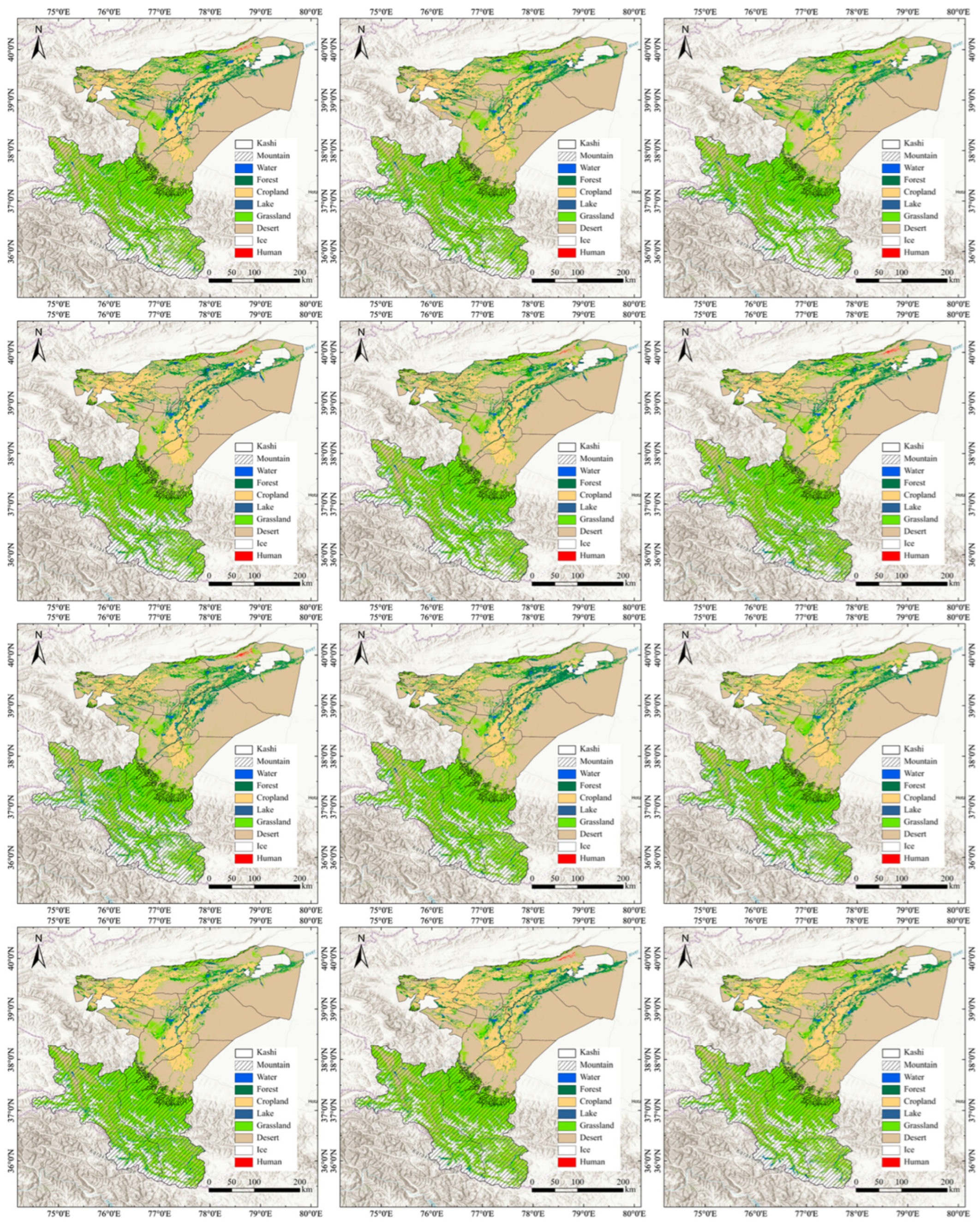
The ecosystem elements exhibited a distinct mountain–oasis–desert spatial pattern in 2026 (Figure 7). The multi-year maps show that the overall spatial structure of ecosystem elements remained broadly stable from 2015 to 2026, although localized changes occurred along oasis margins, river corridors, and Grassland–Desert transition zones (Figure A1). Mountain was mainly distributed in the southwestern and southern high-relief areas, while ice occurred locally at higher elevations. Sensitivity analysis further showed that the broad spatial configuration of the terrain-derived Mountain layer remained stable across the tested parameter combinations. Changes in the relative-relief threshold mainly affected mountain-front and transitional areas, whereas variations in the slope threshold produced negligible changes in Mountain extent (Table A1). Grassland and forest were primarily distributed along mountain margins, lower-elevation slopes, and valleys. Cropland and human-dominated land were concentrated in the central and northern oasis plains and were closely associated with river networks. Water was distributed mainly along river channels, whereas Lake occurred as discrete standing water bodies. Desert occupied extensive areas in the northern, eastern, and southeastern lowlands and formed the dominant ecosystem element. Overall, the spatial distribution showed clear differentiation among the southwestern and southern mountains, the central and northern oases, and the surrounding desert landscapes. Temporal changes were largely confined to transitional and human-dominated areas, while the core distributions of the major ecosystem elements remained relatively stable.
To further quantify these temporal dynamics, annual area statistics were calculated for the eight ecosystem elements, and their interannual variations are shown in Figure 8. The complete annual area statistics for all eight non-mountain ecosystem elements from 2015 to 2026 are provided in Table A2. Desert remained the dominant ecosystem element throughout 2015–2026, but its area declined almost continuously from 69,758 km2 in 2015 to 58,360 km2 in 2026. Accordingly, its share of the study area decreased from 63.1% to 52.8%, a reduction of 10.3 percentage points. The largest reduction occurred before 2021, after which the decline continued at a slower rate, with a slight rebound in 2022. In contrast, the principal vegetated and cultivated classes expanded. Forest increased by 4573 km2 over the study period and its area proportion rose from 5.7% to 9.9%, representing the largest relative increase among the eight classes. Grassland expanded from 12,949 km2 to 16,836 km2, increasing its regional share from 11.7% to 15.2%. Most of this expansion occurred before 2019, followed by moderate interannual fluctuations and a maximum area of 16,975 km2 in 2025. Cropland increased markedly from 9969 km2 in 2015 to 13,214 km2 in 2020 and subsequently remained close to 13,000 km2, reaching 13,237 km2 in 2026. Its proportion therefore increased from 9.0% to 12.0%, indicating that the main cropland expansion occurred during the first half of the study period.
Figure 8.
Temporal changes in the proportional composition of ecosystem elements in the Kashi region from 2015 to 2026.
Ice showed the opposite trajectory, decreasing by 1938 km2 between 2015 and 2026, with its share falling from 5.8% to 4.1%. Despite short-term increases in 2018, 2019, 2023, and 2026, the long-term trend remained negative. Water exhibited stronger interannual variability than the major terrestrial classes, ranging from 2540 km2 in 2016 to 3544 km2 in 2026, while its proportion increased overall from 2.5% to 3.2%. Human-dominated land expanded from 2077 km2 to 2869 km2, with the most pronounced increase occurring between 2019 and 2021; after peaking at 2996 km2 in 2021, it fluctuated within a relatively narrow range. Lake remained the smallest class throughout the study period, accounting for less than 0.1% of the regional area despite increasing from 81 km2 to 103 km2. Overall, the proportional structure was characterized by a substantial contraction of desert, concurrent increases in forest, grassland, and cropland, and a persistent reduction in ice, while water, lake, and human-dominated land contributed only limited changes to the total regional composition.
To further examine the direction and magnitude of ecosystem-element conversions, transition patterns were analyzed for four representative periods from 2015 to 2026 (Figure 9).
Figure 9.
Transition patterns among ecosystem elements in the Kashi region during four periods: (a) 2015–2018, (b) 2018–2021, (c) 2021–2023, and (d) 2023–2026. Chord width represents the magnitude of the transferred area, and chord direction indicates the transition from the initial ecosystem element to the final ecosystem element. Dashed arrows indicate changes in years.
For the transition analysis, mountain was excluded because it was treated as a physiographic layer rather than a surface-cover transition class, while lake was merged into water owing to its small area, limited temporal variation and weak transition signals. The resulting transition matrices for the seven surface-cover ecosystem elements showed a progressive decline in conversion intensity from 2015 to 2026, with the most pronounced restructuring occurring before 2021. The largest change occurred during 2015–2018, when 7649 km2, accounting for 6.9% of the study area, underwent category conversion. During this period, desert decreased substantially, while forest, grassland, and cropland expanded, indicating that the contraction of desert was the principal source of gains in vegetated and cultivated land. Conversion intensity remained relatively high during 2018–2021, with 5896 km2, or 5.34% of the regional area, changing category. Forest and cropland continued to increase, human-dominated land expanded markedly, and desert remained the dominant source of transferred land. After 2021, ecosystem-element transitions weakened considerably. The changed area declined to 2087 km2 during 2021–2023 and 2046 km2 during 2023–2026, corresponding to only 1.9% and 1.8% of the study area, respectively. The 2021–2023 period was characterized by moderate increases in forest and water, accompanied by slight reductions in cropland, grassland, desert, ice, and human-dominated land. During 2023–2026, cropland, grassland, forest, water, and human-dominated land increased slightly, whereas desert and ice continued to decline. Overall, ecosystem-element restructuring was most active before 2021 and subsequently entered a relatively stable stage, with desert contraction and the expansion of vegetated and cultivated land constituting the dominant long-term transition pattern.
4.5. Landscape Pattern Dynamics of Ecosystem Elements in the Kashi Region
To characterize the spatial configuration and temporal dynamics of ecosystem elements in the Kashi region, four class-level landscape metrics were employed: patch density (PD), largest patch index (LPI), landscape shape index (LSI), and edge density (ED). Landscape metrics were calculated for seven major surface-cover ecosystem elements, with mountain excluded and lake merged into water. These metrics respectively describe landscape fragmentation, dominant-patch extent, boundary complexity, and edge intensity. Clear differences in landscape configuration were observed among ecosystem elements from 2015 to 2026 (Figure 10). Grassland consistently exhibited the highest PD and ED, with values of approximately 0.64–0.70 patches km−2 and 55–61 m ha−1, respectively, indicating a highly fragmented pattern with extensive patch boundaries. Its relatively high LPI and LSI further suggest that large grassland patches coexisted with complex and irregular edges. Desert maintained the highest LPI throughout the study period, generally ranging from approximately 18% to 22%, confirming its role as the dominant landscape matrix. Its moderate-to-high PD, LSI, and ED indicate that extensive desert patches were accompanied by complex boundaries, particularly along oasis margins and vegetation transition zones. Forest had a low LPI but relatively high LSI and ED, reflecting a dispersed distribution with complex patch shapes. Cropland showed comparatively low PD and ED, while its LPI increased from approximately 3% in 2015 to more than 5% in 2026, suggesting increasing spatial aggregation within the oasis agricultural areas.
Figure 10.
Temporal variations in class-level landscape pattern metrics of ecosystem elements in the Kashi region from 2015 to 2026.
Temporal changes varied considerably among classes. Grassland PD, LSI, and ED remained high throughout the study period but generally declined after 2021, indicating a moderate reduction in fragmentation and boundary complexity. Desert also showed decreasing PD, LSI, and ED toward 2026, consistent with a simplification of its patch configuration despite its continued landscape dominance. Forest displayed relatively strong temporal fluctuations, particularly in LSI and ED, suggesting continued adjustment of its fragmented spatial pattern. Water and ice had low LPI values but moderate-to-high LSI and ED because of their narrow, elongated, and topographically constrained distributions. Human-dominated land had low PD, LPI, and ED but a relatively high LSI, indicating that its overall extent remained limited while the shapes of artificial patches were comparatively complex. Overall, the landscape structure was dominated by extensive desert and grassland patches, whereas forest, cropland, water, ice, and human-dominated land exhibited smaller and more spatially heterogeneous configurations.
5. Discussion
This study developed an ecosystem-oriented hierarchical classification framework integrating multi-source remote sensing features, terrain constraints, and an adapted ADeFS model. By treating Mountain as an independent physiographic element, the framework reduced semantic overlap between terrain units and surface-cover categories, which is particularly relevant in heterogeneous mountain-oasis-desert systems where topographic position and elevation gradients strongly regulate ecosystem differentiation [46,47]. This hierarchical representation is also consistent with the ecological-community concept that emphasizes the functional relationships among mountains, rivers, forests, farmlands, lakes, grasslands, and deserts rather than treating them as isolated land-cover classes [9,32]. ADeFS achieved the highest performance among the five evaluated models, with an OA of 88.7% and a Kappa coefficient of 0.868, while independent field validation yielded an OA of 86.2% and a Kappa coefficient of 0.825. Although the OA improvement over the benchmark classifiers was relatively moderate, pairwise McNemar tests showed that the differences in prediction outcomes were statistically significant for all four comparisons. In particular, SVM achieved the closest OA to ADeFS, but their paired prediction results still differed significantly (p = 0.001). Moreover, the number of samples correctly classified by ADeFS but misclassified by the benchmark models was consistently greater than the number showing the opposite outcome, providing additional statistical support for the observed performance advantage of ADeFS.
The performance of ADeFS can be associated with the cascade-based representation learning of deep forests and the shrinkage mechanism used to reduce redundant model components [43,44]. Feature importance was concentrated in NDVI, terrain roughness, SAVI, NDWI, and B7, which together accounted for 74.8% of the total importance. This result highlights the importance of vegetation condition, surface moisture, shortwave-infrared information, and terrain heterogeneity in distinguishing ecosystem elements. Previous studies have similarly demonstrated the value of harmonized optical observations, SAR-derived vegetation information, and terrain variables for characterizing heterogeneous land surfaces [40]. The relatively low individual importance of VV, VH, and VV/VH in this study suggests that SAR backscatter contributed less directly under the current feature configuration, while the lower accuracies of forest and grassland indicate that vegetation-related and transitional surfaces remain major sources of classification uncertainty.
The observed temporal changes are broadly consistent with previous studies of land-use and ecological change in the Kashi region. Long-term remote-sensing analyses have documented persistent oasis expansion, agricultural development, and increasing human influence in Kashi [48,49]. Studies in the Kashi River Basin have also revealed substantial land-cover restructuring in piedmont and oasis-transition areas, although the trajectories of vegetation classes vary with the study period and classification scheme [50,51]. In this study, cropland increased from 9969 km2 to 13,237 km2, while forest and grassland increased by 4573 km2 and 3887 km2, respectively, whereas desert decreased by 11,398 km2. These changes should not be interpreted solely as ecological restoration because oasis expansion and irrigation may also alter soil and hydrological conditions [52]. Previous studies have identified widespread and dynamic soil salinization in the Kashi oasis and Kashi River Basin, driven jointly by groundwater, topography, irrigation, vegetation, and other human activities [53,54]. Meanwhile, the decline in Ice observed in this study is consistent with recent evidence of glacier retreat in the Pamir Plateau after 2015 [55]. In our classification scheme, the Ice class includes glaciers, permanent snow, and other persistent frozen surfaces; therefore, its decline should not be interpreted solely as glacier-area loss. Regional glacier dynamics are largely controlled by increasing air temperatures and stronger ablation processes, although snowfall variability, debris cover, topography, and glacier dynamics can produce substantial spatial differences in glacier response [56]. Such changes have important hydrological implications because glacier and snowmelt contribute to downstream runoff in the arid basins of western High Mountain Asia [57]. Enhanced melting may temporarily increase meltwater supply, whereas continued loss of glacier ice reduces long-term solid-water storage and may increase the vulnerability of downstream water resources [58].
The landscape metrics further reveal that ecosystem-element changes involved not only variations in area but also adjustments in spatial configuration. Desert maintained the highest LPI, confirming its role as the dominant landscape matrix, whereas grassland exhibited the highest PD and ED, indicating extensive but highly fragmented patches. However, given the comparatively low User’s Accuracy of Grassland in the independent validation, these metrics should be interpreted with caution. Part of the apparent fragmentation may reflect classification uncertainty and boundary-related misclassification rather than ecological fragmentation alone. The increasing LPI of cropland suggests greater spatial aggregation within oasis agricultural areas, while the low LPI and high LSI of forest reflect a dispersed distribution with complex boundaries. Similar landscape restructuring has been reported in the Kashi River Basin and other arid oases of southern Xinjiang, where agricultural expansion, urbanization, irrigation development, and oasis–desert interactions substantially altered patch fragmentation, aggregation, and connectivity [59,60]. Studies in Kashi City have also identified relatively high fragmentation and weak connectivity in urban green-space systems, indicating strong spatial heterogeneity within human-dominated oasis landscapes [61]. At the regional scale, landscape-pattern-based ecological risk assessments further highlight the importance of grassland, desert, cropland, and ice in shaping ecological risk across the Kashi Region [62]. The general decline in PD, LSI, and ED after 2021 in the present study therefore suggests a recent weakening of landscape restructuring, although this short-term trend should be interpreted within the longer-term history of fragmentation and land-use reorganization in the region.
Several limitations should be acknowledged. The consensus samples may retain uncertainties inherited from the source land-cover products, as discrepancies among existing land-cover datasets can arise from differences in classification systems, spatial resolution, and mapping accuracy [63]. In addition, uncertainty in reference data can propagate into both classification and accuracy assessment, particularly when field observations are spatially limited [64]. The independent field survey in this study covered only six accessible classes, excluding mountain, lake, and ice. Although several field routes passed through mountainous areas and provided qualitative confirmation of the broad Mountain distribution, no dedicated Mountain/non-Mountain reference dataset was established; therefore, the terrain-derived Mountain boundary remains without independent quantitative validation. The multi-source reference products used for sample construction were available for 2015–2020, whereas comparable annual products were not consistently available for 2021–2025. Consequently, no independent reference data were available to directly assess the annual classification accuracy for these intermediate years, and the corresponding maps should be interpreted as model-based temporal mapping results rather than independently validated annual products. Moreover, the annual maps were classified independently without explicit temporal-continuity constraints, which may introduce artificial interannual fluctuations; similar temporal inconsistencies have been identified in independently generated annual land-cover sequences [65]. Future work should incorporate higher-resolution imagery, broader field observations, and spatiotemporal learning methods, while extending ecological constraints to hydrological and cryospheric elements and examining connectivity, ecosystem services, and interactions among ecosystem elements.
6. Conclusions
This study developed an ecosystem-oriented hierarchical classification framework for the Kashi region using multi-source remote sensing data, terrain constraints, and an adapted ADeFS model. Mountain was extracted as an independent physiographic element before the remaining ecosystem elements were classified. ADeFS achieved the highest performance among the five models, with an OA of 88.7% and a Kappa coefficient of 0.868. Independent field validation of the 2026 map yielded an OA of 86.2% and a Kappa coefficient of 0.825. From 2015 to 2026, the overall mountain–oasis–desert pattern remained stable. Desert and ice decreased, while forest, grassland, and cropland expanded. Ecosystem-element transitions were concentrated before 2021 and weakened thereafter. Landscape metrics showed that desert remained the dominant matrix, grassland had the highest fragmentation and edge intensity, and cropland became more spatially aggregated. The proposed framework provides an effective approach for ecosystem-element mapping in arid and heterogeneous regions. Further improvement is needed in field-sample coverage, temporal consistency, and the classification of transitional surfaces.
Author Contributions
Conceptualization, methodology, software, formal analysis, investigation, data curation, visualization, and writing—original draft preparation: L.J.; methodology, validation, and writing—review and editing: W.W.; resources, supervision, project administration, and funding acquisition: X.L.; conceptualization, supervision, validation, writing—review and editing, and funding acquisition: G.J.M.P.; validation and investigation: Y.X. All authors have read and agreed to the published version of the manuscript.
Funding
This research was funded by the Kashi Science and Technology Plan Project (KS2024012), Key Technologies for the Application of Aerospace Big Data Resources and Environment to Monitor and Evaluate Sustainable Development Goals; Shanghai Cooperation Organization Science and Technology Partnership Program and International Science and Technology Cooperation Program (2025E01041), Remote Sensing Assessment and Capacity Building for Sustainable Development in China–Kyrgyzstan–Uzbekistan Regions.
Data Availability Statement
The data presented in this study are available on request from the corresponding author.
Acknowledgments
The authors would like to thank all collaborators and colleagues who provided valuable support and constructive suggestions during this study. The authors have reviewed and edited the output and take full responsibility for the content of this publication.
Conflicts of Interest
The authors declare no conflicts of interest.
Abbreviations
The following abbreviations are used in this manuscript:
| ADeFS | Automatic Deep Forest Shrinkage model |
| RF | Random Forest |
| SVM | Support Vector Machine |
| MLP | Multilayer Perceptron |
| OA | Overall Accuracy |
| UA | User’s Accuracy |
| PA | Producer’s Accuracy |
| PD | Patch Density |
| LPI | Largest Patch Index |
| ED | Edge Density |
| LSI | Landscape Shape Index |
Appendix A
Appendix A.1. Sensitivity Analysis of Terrain-Based Mountain Delineation
The sensitivity of the terrain-derived Mountain layer to relative-relief and slope thresholds was evaluated using nine parameter combinations. The original thresholds of 200 m relative relief and 5° slope were used as the baseline configuration, while all other parameters, including the 2 km-radius neighborhood, TPI criterion, 60 m morphological smoothing radius, and 0.5 ha minimum patch-area threshold, were kept unchanged. Relative area change was calculated with respect to the baseline Mountain area, and IoU denotes the intersection-over-union between each parameter-derived Mountain mask and the baseline mask. The results showed that Mountain delineation was highly insensitive to the tested slope thresholds. At a relative-relief threshold of 200 m, changing the slope threshold from 3° to 7° altered the Mountain area by less than 0.01%, with IoU values exceeding 0.9999. In comparison, varying the relative-relief threshold from 150 to 250 m produced moderate changes in Mountain extent, while spatial agreement with the baseline remained approximately 0.87 or higher. These differences mainly reflected expansion or contraction along the mountain front and transitional terrain rather than substantial changes in the overall spatial configuration of the Mountain layer.
Table A1.
Sensitivity of terrain-based Mountain delineation to relative-relief and slope thresholds.
Appendix A.2. Spatial Distribution of Ecosystem Elements from 2015 to 2026
To provide a more detailed view of the temporal evolution of ecosystem elements, the annual classification maps from 2015 to 2026 are presented in Figure A1. Mountain remained concentrated in the southwestern and southern parts of the region, while desert consistently dominated the northern, eastern, and southeastern lowlands. Grassland was distributed mainly along mountain margins and piedmont areas, whereas cropland and human-dominated lands were concentrated in the central and northern oasis plains. Overall, temporal changes were largely confined to transitional and human-dominated areas, while the core distributions of the major ecosystem elements remained relatively stable.
Appendix A.3. Changes in the Areas of Major Ecosystem Elements in the Kashi Region from 2015 to 2026
To further quantify the long-term changes in ecosystem elements, Table A2 summarizes the annual areas of the eight non-mountain ecosystem elements from 2015 to 2026, together with their net changes over the entire study period. The results indicate an overall expansion of cropland, forest, grassland, water, and human-dominated land, accompanied by substantial decreases in desert and ice. Among all ecosystem elements, forests exhibited the largest relative increase, whereas desert land showed the greatest absolute decline.
Table A2.
Annual area statistics and overall changes in the eight non-mountain ecosystem elements in the Kashi region from 2015 to 2026. The rate of change is based on the 2015 area.
Figure A1.
Spatial distribution of ecosystem elements in the Kashi region from 2015 to 2026, arranged chronologically from the upper left to the lower right.
References
- Haddad, N.M.; Brudvig, L.A.; Clobert, J.; Davies, K.F.; Gonzalez, A.; Holt, R.D.; Lovejoy, T.E.; Sexton, J.O.; Austin, M.P.; Collins, C.D.; et al. Habitat fragmentation and its lasting impact on Earth’s ecosystems. Sci. Adv. 2015, 1, e1500052. [Google Scholar] [CrossRef] [Scilit] [PubMed]
- Ipbes. Global Assessment Report on Biodiversity and Ecosystem Services; Intergovernmental Science-Policy Platform on Biodiversity and Ecosystem Services: Bonn, Germany, 2019.
- United Nations General Assembly. United Nations Decade on Ecosystem Restoration (2021–2030): Resolution Adopted by the General Assembly; United Nations: New York, NY, USA, 2019. [Google Scholar]
- Zhai, J.; Wang, L.; Liu, Y.; Wang, C.; Mao, X. Assessing the effects of China’s Three-North Shelter Forest Program over 40 years. Sci. Total Environ. 2023, 857, 159354. [Google Scholar] [CrossRef] [Scilit]
- Ma, Z.; Xia, C.; Cao, S. Cost–Benefit Analysis of China’s Natural Forest Conservation Program. J. Nat. Conserv. 2020, 55, 125818. [Google Scholar] [CrossRef] [Scilit]
- Liu, J.; Li, S.; Ouyang, Z.; Tam, C.; Chen, X. Ecological and socioeconomic effects of China’s policies for ecosystem services. Proc. Natl. Acad. Sci. USA 2008, 105, 9477–9482. [Google Scholar] [CrossRef] [Scilit] [PubMed]
- Fu, B.; Liu, Y.; Meadows, M.E. Ecological restoration for sustainable development in China. Natl. Sci. Rev. 2023, 10, nwad033. [Google Scholar] [CrossRef] [Scilit]
- Song, W.; Feng, Y.; Wang, Z. Ecological restoration programs dominate vegetation greening in China. Sci. Total Environ. 2022, 848, 157729. [Google Scholar] [CrossRef] [Scilit]
- Liu, S.; Dong, Y.; McConkey, K.R.; Tran, L.-S.P.; Wang, F.; Liu, H.; Wu, G. Scientific concept and practices of life community of mountains, rivers, forests, farmlands, lakes, grasslands, and deserts in China. Ambio 2023, 52, 1939–1951. [Google Scholar] [CrossRef] [Scilit]
- Zhou, Y.; Li, Y.; Li, W.; Li, F.; Xin, Q. Ecological Responses to Climate Change and Human Activities in the Arid and Semi-Arid Regions of Xinjiang in China. Remote Sens. 2022, 14, 3911. [Google Scholar] [CrossRef] [Scilit]
- Maimaitiaili, A.; Aji, X.; Matniyaz, A.; Kondoh, A. Monitoring and Analysing Land Use/Cover Changes in an Arid Region Based on Multi-Satellite Data: The Kashgar Region, Northwest China. Land 2018, 7, 6. [Google Scholar] [CrossRef] [Scilit]
- Chen, R.; Yang, H.; Yang, G.; Liu, Y.; Zhang, C.; Long, H.; Xu, H.; Meng, Y.; Feng, H. Land-Use Mapping with Multi-Temporal Sentinel Images Based on Google Earth Engine in Southern Xinjiang Uygur Autonomous Region, China. Remote Sens. 2023, 15, 3958. [Google Scholar] [CrossRef] [Scilit]
- Ding, C.; Ren, C. Monitoring Water Area Dynamics in Kashgar (2003–2023) Using Multi-Source Remote Sensing Data. Appl. Sci. 2025, 15, 5194. [Google Scholar] [CrossRef] [Scilit]
- Keith, D.A.; Ferrer-Paris, J.R.; Nicholson, E.; Bishop, M.J.; Polidoro, B.A.; Ramirez-Llodra, E.; Tozer, M.G.; Nel, J.L.; Mac Nally, R.; Gregr, E.J.; et al. A Function-Based Typology for Earth’s Ecosystems. Nature 2022, 610, 513–518. [Google Scholar] [CrossRef] [Scilit] [PubMed]
- Wang, H.; Yang, H.; Huang, Y.; Wu, L.; Guo, Z.; Li, N. Classification of Land Cover in Complex Terrain Using Gaofen-3 SAR Ascending and Descending Orbit Data. Remote Sens. 2023, 15, 2177. [Google Scholar] [CrossRef] [Scilit]
- Li, J.; Hong, D.; Gao, L.; Yao, J.; Zheng, K.; Zhang, B.; Chanussot, J. Deep Learning in Multimodal Remote Sensing Data Fusion: A Comprehensive Review. Int. J. Appl. Earth Obs. Geoinf. 2022, 112, 102926. [Google Scholar] [CrossRef] [Scilit]
- Laliberte, A.S.; Fredrickson, E.L.; Rango, A. Combining Decision Trees with Hierarchical Object-oriented Image Analysis for Mapping Arid Rangelands. Photogramm. Eng. Remote Sens. 2007, 73, 197–207. [Google Scholar] [CrossRef] [Scilit]
- Ge, G.; Shi, Z.; Zhu, Y.; Yang, X.; Hao, Y. Land use/cover classification in an arid desert-oasis mosaic landscape of China using remote sensed imagery: Performance assessment of four machine learning algorithms. Glob. Ecol. Conserv. 2020, 22, e00971. [Google Scholar] [CrossRef] [Scilit]
- Yang, A.; Zhong, B.; Wang, X.; Feng, A.; Hu, L.; Ao, K.; Zhai, Q.; Wu, S.; Du, B.; Wu, J. 30 m 5-yearly land cover maps of Qilian Mountain Area (QMA_LC30) from 1990 to 2020. Sci. Data 2024, 11, 1339. [Google Scholar] [CrossRef] [Scilit]
- Yang, Q.; Zhou, X.; Spengler, R.N.; Zhao, K.; Liu, J.; Bao, Y.; Jia, P.W.; Li, X. Prehistoric agriculture and social structure in the southwestern Tarim Basin: Multiproxy analyses at Wupaer. Sci. Rep. 2020, 10, 14235. [Google Scholar] [CrossRef] [Scilit]
- Yi, S.; Wang, H.; Wang, C.; Huang, X. Threshold Effects and Synergistic Trade-Offs in Ecosystem Services: A Spatio-Temporal Study of Kashgar’s Arid Region. Agriculture 2025, 15, 1742. [Google Scholar] [CrossRef] [Scilit]
- Aimaiti, M.; Meng, X. Multi-decadal landscape dynamics and ecological security trajectories driven by 43-year land use changes in Kashgar, an arid border region of Northwest China. Sci. Rep. 2026, 16, 20495. [Google Scholar] [CrossRef] [Scilit]
- Clinton, N.; Yu, L.; Gong, P. Geographic stacking: Decision fusion to increase global land cover map accuracy. ISPRS J. Photogramm. Remote Sens. 2015, 103, 57–65. [Google Scholar] [CrossRef] [Scilit]
- Ju, J.; Zhou, Q.; Freitag, B.; Roy, D.P.; Zhang, H.K.; Sridhar, M.; Mandel, J.; Arab, S.; Schmidt, G.L.; Crawford, C.J.; et al. The Harmonized Landsat and Sentinel-2 version 2.0 surface reflectance dataset. Remote Sens. Environ. 2025, 324, 114723. [Google Scholar] [CrossRef] [Scilit]
- Torres, R.; Snoeij, P.; Geudtner, D.; Bibby, D.; Davidson, M.; Attema, E.; Potin, P.; Rommen, B.; Floury, N.; Brown, M.; et al. GMES Sentinel-1 mission. Remote Sens. Environ. 2012, 120, 9–24. [Google Scholar] [CrossRef] [Scilit]
- Farr, T.G.; Rosen, P.A.; Caro, E.; Crippen, R.; Duren, R.; Hensley, S.; Kobrick, M.; Paller, M.; Rodriguez, E.; Roth, L.; et al. The Shuttle Radar Topography Mission. Rev. Geophys. 2007, 45, RG2004. [Google Scholar] [CrossRef] [Scilit]
- Zhang, X.; Liu, L.; Chen, X.; Gao, Y.; Xie, S.; Mi, J. GLC_FCS30: Global land-cover product with fine classification system at 30 m using time-series Landsat imagery. Earth Syst. Sci. Data 2021, 13, 2753–2776. [Google Scholar] [CrossRef] [Scilit]
- Yang, J.; Huang, X. The 30 m annual land cover dataset and its dynamics in China from 1990 to 2019. Earth Syst. Sci. Data 2021, 13, 3907–3925. [Google Scholar] [CrossRef] [Scilit]
- Zanaga, D.; Van De Kerchove, R.; De Keersmaecker, W.; Souverijns, N.; Brockmann, C.; Quast, R.; Wevers, J.; Grosu, A.; Paccini, A.; Vergnaud, S.; et al. ESA WorldCover 10 m 2020 v100. Zenodo 2021. [Google Scholar] [CrossRef]
- Sulla-Menashe, D.; Gray, J.M.; Abercrombie, S.P.; Friedl, M.A. Hierarchical mapping of annual global land cover 2001 to present: The MODIS Collection 6 Land Cover product. Remote Sens. Environ. 2019, 222, 183–194. [Google Scholar] [CrossRef] [Scilit]
- Olofsson, P.; Foody, G.M.; Herold, M.; Stehman, S.V.; Woodcock, C.E.; Wulder, M.A. Good Practices for Estimating Area and Assessing Accuracy of Land Change. Remote Sens. Environ. 2014, 148, 42–57. [Google Scholar] [CrossRef] [Scilit]
- Li, Y.; Hu, Y.; Wang, Z. Mountain-water-forest-farmland-lake-grassland-sandland holistic protection and restoration engineering and landscape ecology. Chin. J. Appl. Ecol. 2023, 34, 249–256. [Google Scholar] [CrossRef] [Scilit]
- Wu, J. Landscape sustainability science: Ecosystem services and human well-being in changing landscapes. Landsc. Ecol. 2013, 28, 999–1023. [Google Scholar] [CrossRef] [Scilit]
- Claverie, M.; Ju, J.; Masek, J.G.; Dungan, J.L.; Vermote, E.F.; Roger, J.-C.; Skakun, S.V.; Justice, C. The Harmonized Landsat and Sentinel-2 surface reflectance data set. Remote Sens. Environ. 2018, 219, 145–161. [Google Scholar] [CrossRef] [Scilit]
- McFeeters, S.K. The use of the Normalized Difference Water Index (NDWI) in the delineation of open water features. Int. J. Remote Sens. 1996, 17, 1425–1432. [Google Scholar] [CrossRef] [Scilit]
- Tucker, C.J. Red and photographic infrared linear combinations for monitoring vegetation. Remote Sens. Environ. 1979, 8, 127–150. [Google Scholar] [CrossRef] [Scilit]
- Huete, A.R. A soil-adjusted vegetation index (SAVI). Remote Sens. Environ. 1988, 25, 295–309. [Google Scholar] [CrossRef] [Scilit]
- Lee, J.-S.; Pottier, E. Polarimetric Radar Imaging: From Basics to Applications; CRC Press: Boca Raton, FL, USA, 2009. [Google Scholar]
- Nasirzadehdizaji, R.; Balik Sanli, F.; Abdikan, S.; Cakir, Z.; Sekertekin, A.; Ustuner, M. Sensitivity analysis of multi-temporal Sentinel-1 SAR parameters to crop height and canopy coverage. Appl. Sci. 2019, 9, 655. [Google Scholar] [CrossRef] [Scilit]
- Mandal, D.; Kumar, V.; Ratha, D.; Dey, S.; Bhattacharya, A.; Lopez-Sanchez, J.M.; McNairn, H.; Rao, Y.S. Dual polarimetric radar vegetation index for crop growth monitoring using Sentinel-1 SAR data. Remote Sens. Environ. 2020, 247, 111954. [Google Scholar] [CrossRef] [Scilit]
- Wood, J.D. The Geomorphological Characterisation of Digital Elevation Models. Ph.D. Thesis, University of Leicester, Leicester, UK, 1996. [Google Scholar]
- Weiss, A.D. Topographic Position and Landforms Analysis. In Proceedings of the ESRI International User Conference, San Diego, CA, USA, 9–13 July 2001. [Google Scholar]
- Farhadi, Z.; Feizi-Derakhshi, M.-R.; Khalaf Salman Al-Tameemi, I.; Kim, W. ADeFS: A Deep Forest Regression-Based Model to Enhance the Performance Based on LASSO and Elastic Net. Mathematics 2025, 13, 118. [Google Scholar] [CrossRef] [Scilit]
- Zhou, Z.-H.; Feng, J. Deep Forest: Towards An Alternative to Deep Neural Networks. In Proceedings of the Twenty-Sixth International Joint Conference on Artificial Intelligence, Melbourne, Australia, 19–25 August 2017; pp. 3553–3559. [Google Scholar]
- Zou, H.; Hastie, T. Regularization and Variable Selection Via the Elastic Net. J. R. Stat. Soc. Ser. B Stat. Methodol. 2005, 67, 301–320. [Google Scholar] [CrossRef] [Scilit]
- Körner, C. The use of altitude in ecological research. Trends Ecol. Evol. 2007, 22, 569–574. [Google Scholar] [CrossRef] [Scilit] [PubMed]
- De Reu, J.; Bourgeois, J.; Bats, M.; Zwertvaegher, A.; Gelorini, V.; De Smedt, P.; Chu, W.; Antrop, M.; De Maeyer, P.; Finke, P.; et al. Application of the topographic position index to heterogeneous landscapes. Geomorphology 2013, 186, 39–49. [Google Scholar] [CrossRef] [Scilit]
- Mamat, A.; Halik, Ü.; Rouzi, A. Variations of Ecosystem Service Value in Response to Land-Use Change in the Kashgar Region, Northwest China. Sustainability 2018, 10, 200. [Google Scholar] [CrossRef] [Scilit]
- Maimaiti, B.; Chen, S.; Kasimu, A.; Mamat, A.; Aierken, N.; Chen, Q. Coupling and Coordination Relationships between Urban Expansion and Ecosystem Service Value in Kashgar City. Remote Sens. 2022, 14, 2557. [Google Scholar] [CrossRef] [Scilit]
- Kulaixi, Z.; Chen, Y.; Li, Y.; Wang, C. Dynamic Evolution and Scenario Simulation of Ecosystem Services under the Impact of Land-Use Change in an Arid Inland River Basin in Xinjiang, China. Remote Sens. 2023, 15, 2476. [Google Scholar] [CrossRef] [Scilit]
- Wei, T.; Shangguan, D.; Shen, X.; Ding, Y.; Yi, S. Dynamics of Land Use and Land Cover Changes in An Arid Piedmont Plain in the Middle Reaches of the Kaxgar River Basin, Xinjiang, China. ISPRS Int. J. Geo-Inf. 2020, 9, 87. [Google Scholar] [CrossRef] [Scilit]
- Ran, H.; Ma, Y.; Xu, Z. Evaluation and Prediction of Land Use Ecological Security in the Kashgar Region Based on Grid GIS. Sustainability 2022, 15, 40. [Google Scholar] [CrossRef] [Scilit]
- Lv, T.; Liu, Y.; Bian, M.; Zhang, X.; Chen, C.; Wang, M. Spatial Distribution and Temporal Evolution of Soil Salinization in the Oasis Irrigated Area. Agronomy 2025, 15, 2413. [Google Scholar] [CrossRef] [Scilit]
- Li, S.; Lu, L.; Gao, Y.; Zhang, Y.; Shen, D. An Analysis on the Characteristics and Influence Factors of Soil Salinity in the Wasteland of the Kashgar River Basin. Sustainability 2022, 14, 3500. [Google Scholar] [CrossRef] [Scilit]
- Han, Y.; Wang, Y.; Ma, X.; Shang, Y. Glacier and Snow Cover Dynamics and Their Affecting Factors on the Pamir Plateau Section of the China-Pakistan Economic Corridor. Land 2025, 14, 880. [Google Scholar] [CrossRef] [Scilit]
- Xie, F.; Liu, S.; Gao, Y.; Zhu, Y.; Bolch, T.; Kääb, A. Interdecadal glacier inventories in the Karakoram since the 1990s. Earth Syst. Sci. Data 2023, 15, 847–867. [Google Scholar] [CrossRef] [Scilit]
- Pohl, E.; Gloaguen, R.; Andermann, C.; Knoche, M. Glacier melt buffers river runoff in the Pamir Mountains. Water Resour. Res. 2017, 53, 2467–2489. [Google Scholar] [CrossRef] [Scilit]
- Su, F.; Pritchard, H.D.; Yao, T.; Huang, J.; Ou, T.; Meng, F.; Sun, H.; Li, Y.; Xu, B.; Zhu, M.; et al. Contrasting Fate of Western Third Pole’s Water Resources Under 21st Century Climate Change. Earth’s Future 2022, 10, e2022EF002776. [Google Scholar] [CrossRef] [Scilit]
- Xue, J.; Gui, D.; Zeng, F.; Yu, X.; Sun, H.; Zhang, J.; Liu, Y.; Xue, D. Assessing landscape fragmentation in a desert-oasis region of Northwest China: Patterns, driving forces, and policy implications for future land consolidation. Environ. Monit. Assess. 2022, 194, 394. [Google Scholar] [CrossRef] [Scilit]
- Zhang, L.; Liu, Y.; Yin, C.; Xue, D.; Gui, D.; Qi, Z. Effects of Farmland Landscape Fragmentation on Agricultural Irrigation in Hotan Oasis. Agriculture 2022, 12, 1503. [Google Scholar] [CrossRef] [Scilit]
- Li, X.; Xia, G.; Lin, T.; Xu, Z.; Wang, Y. Construction of Urban Green Space Network in Kashgar City, China. Land 2022, 11, 1826. [Google Scholar] [CrossRef] [Scilit]
- Yang, G.; Ma, G. Ecological risk assessment of land use in Kashgar Prefecture based on landscape pattern. Anhui Agric. Sci. Bull. 2025, 31, 95–99. [Google Scholar] [CrossRef]
- Herold, M.; Mayaux, P.; Woodcock, C.E.; Baccini, A.; Schmullius, C. Some challenges in global land cover mapping: An assessment of agreement and accuracy in existing 1 km datasets. Remote Sens. Environ. 2008, 112, 2538–2556. [Google Scholar] [CrossRef] [Scilit]
- Foody, G.M. Assessing the accuracy of land cover change with imperfect ground reference data. Remote Sens. Environ. 2010, 114, 2271–2285. [Google Scholar] [CrossRef] [Scilit]
- Liu, S.; Su, H.; Cao, G.; Wang, S.; Guan, Q. Learning from data: A post classification method for annual land cover analysis in urban areas. ISPRS J. Photogramm. Remote Sens. 2019, 154, 202–215. [Google Scholar] [CrossRef] [Scilit]
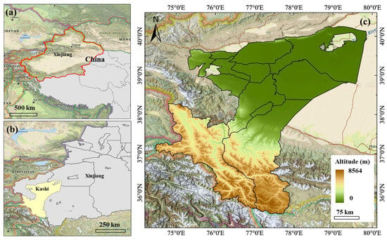
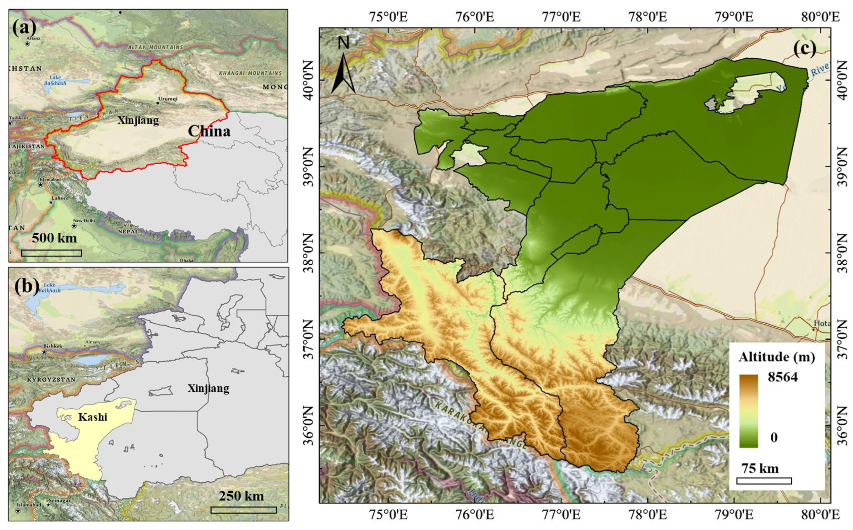
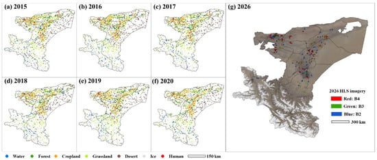
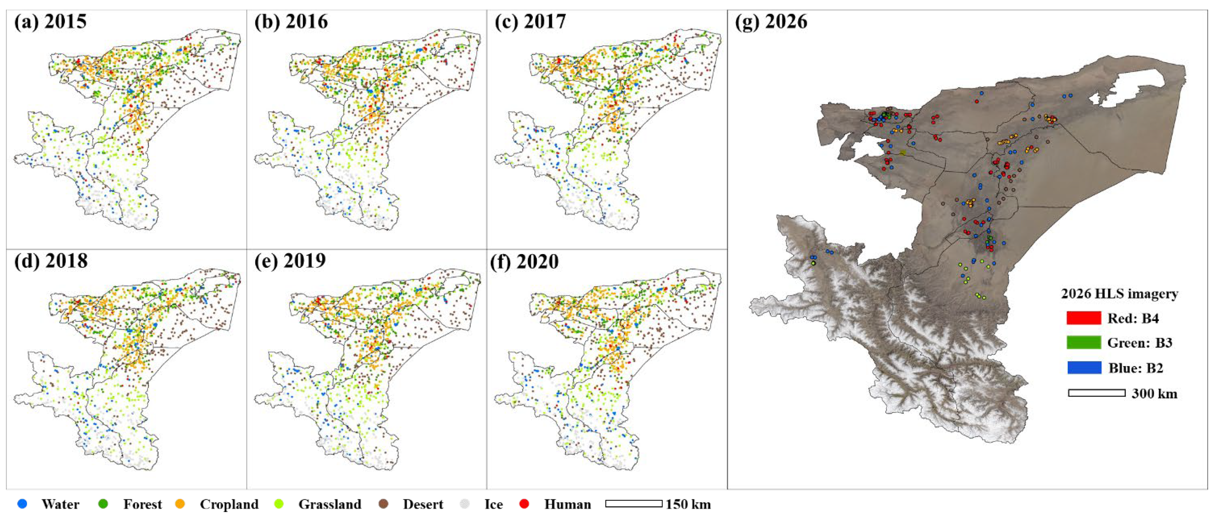
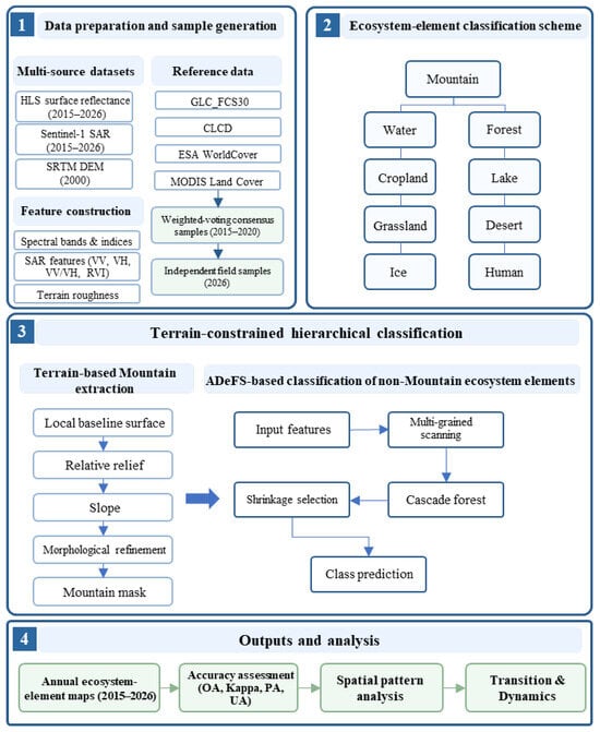
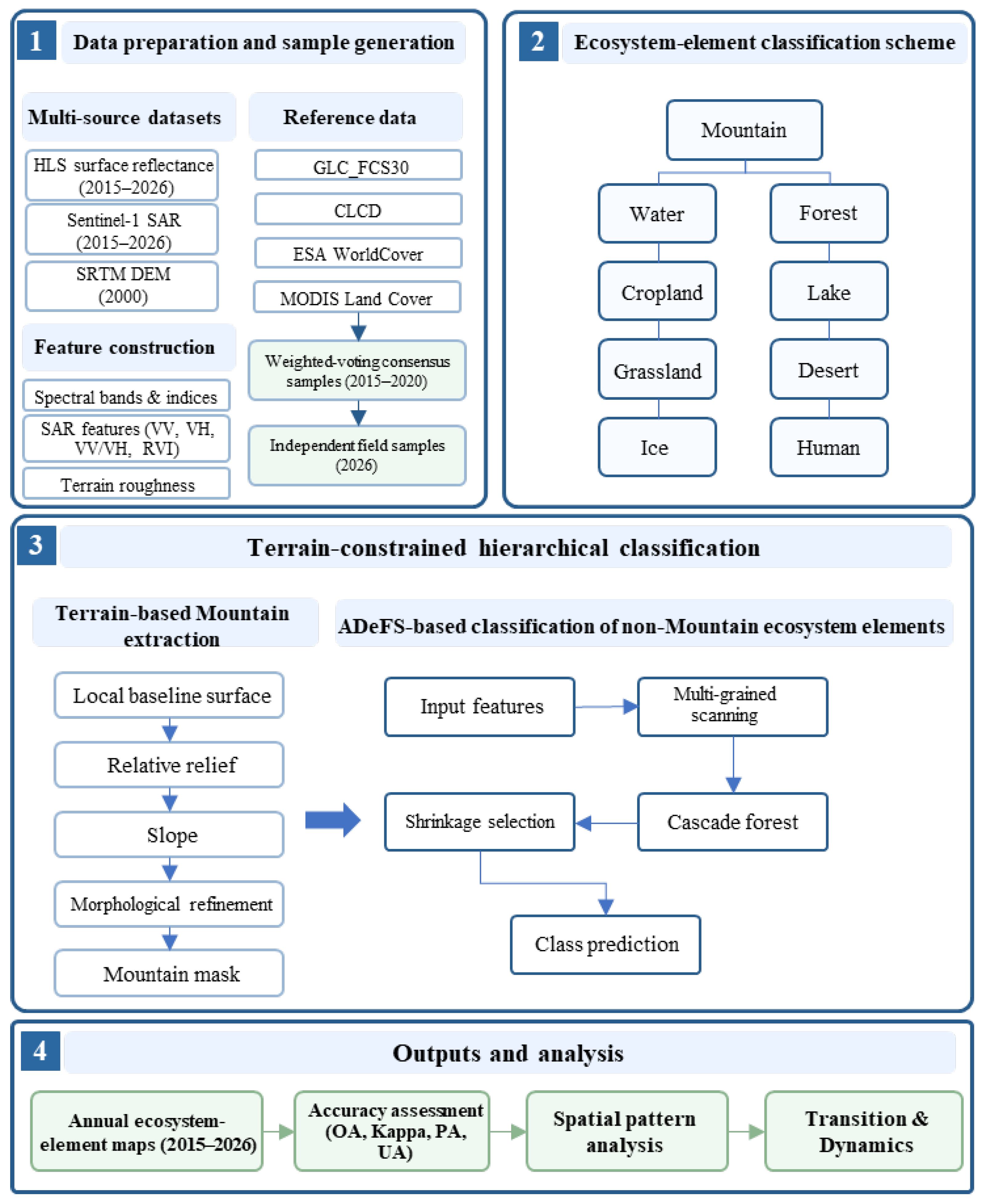
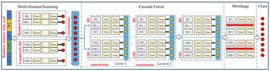
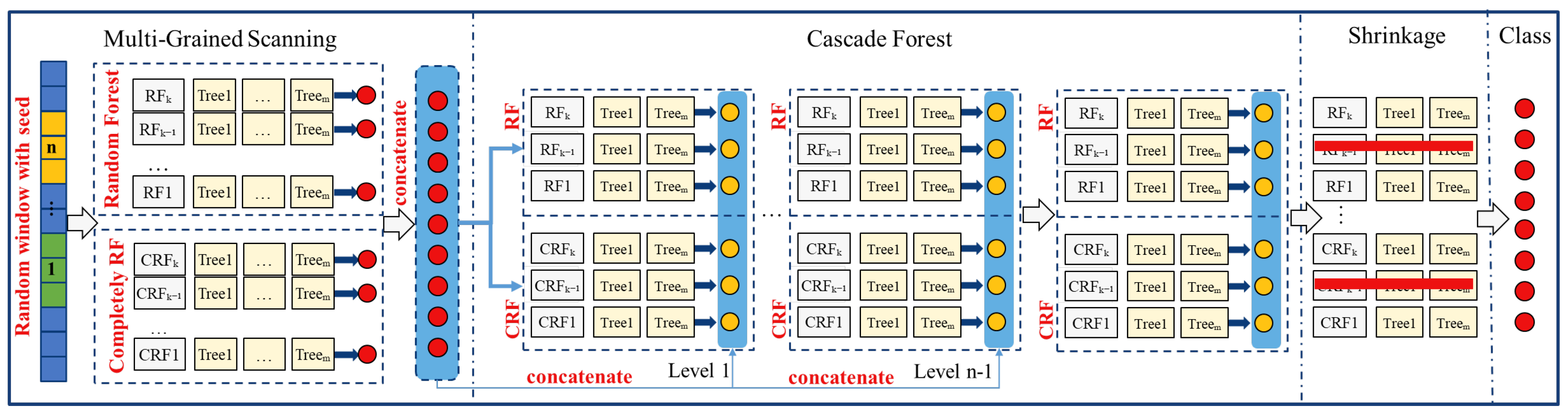
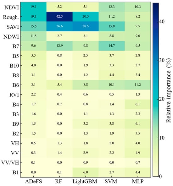
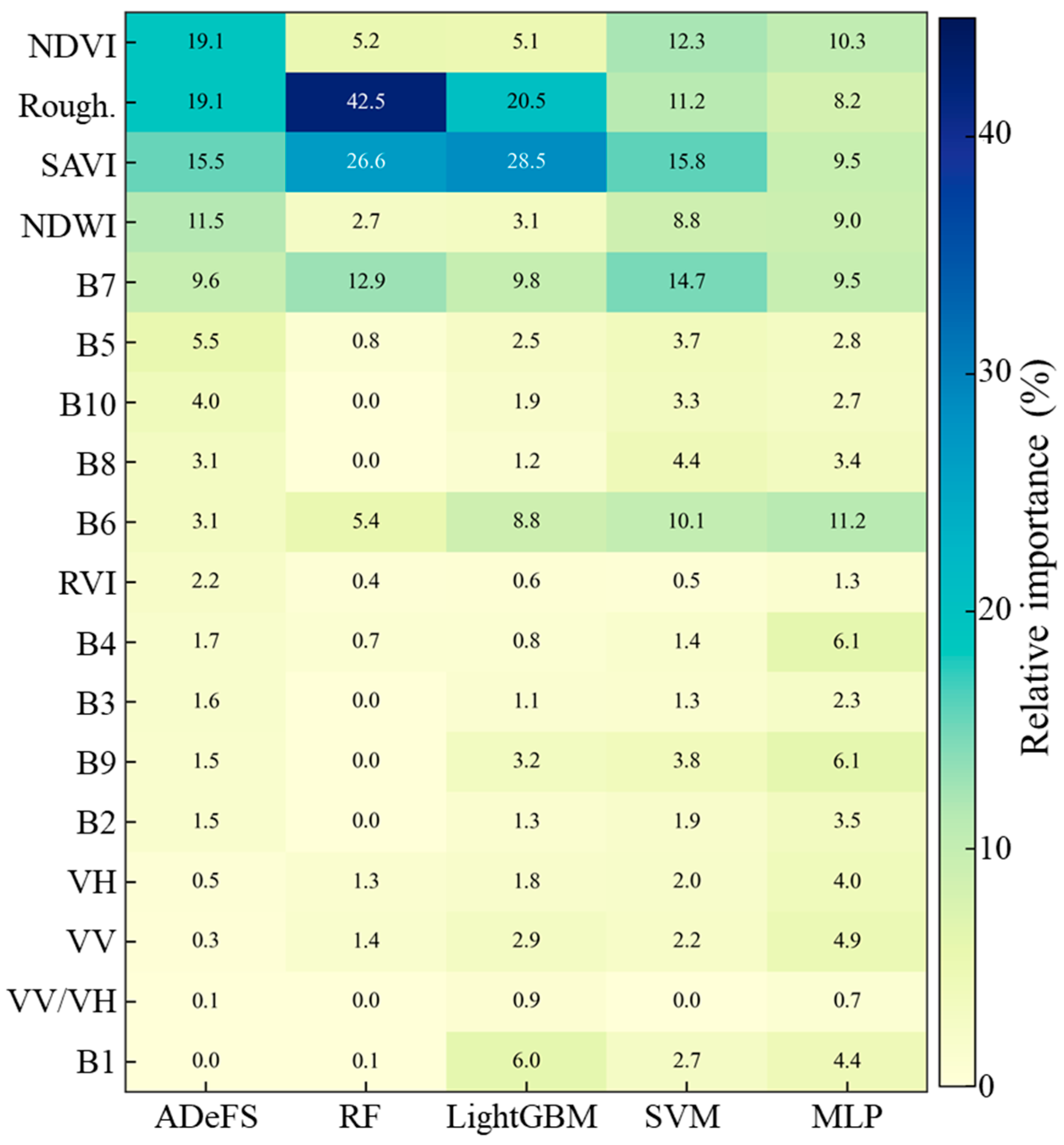
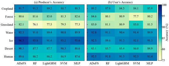
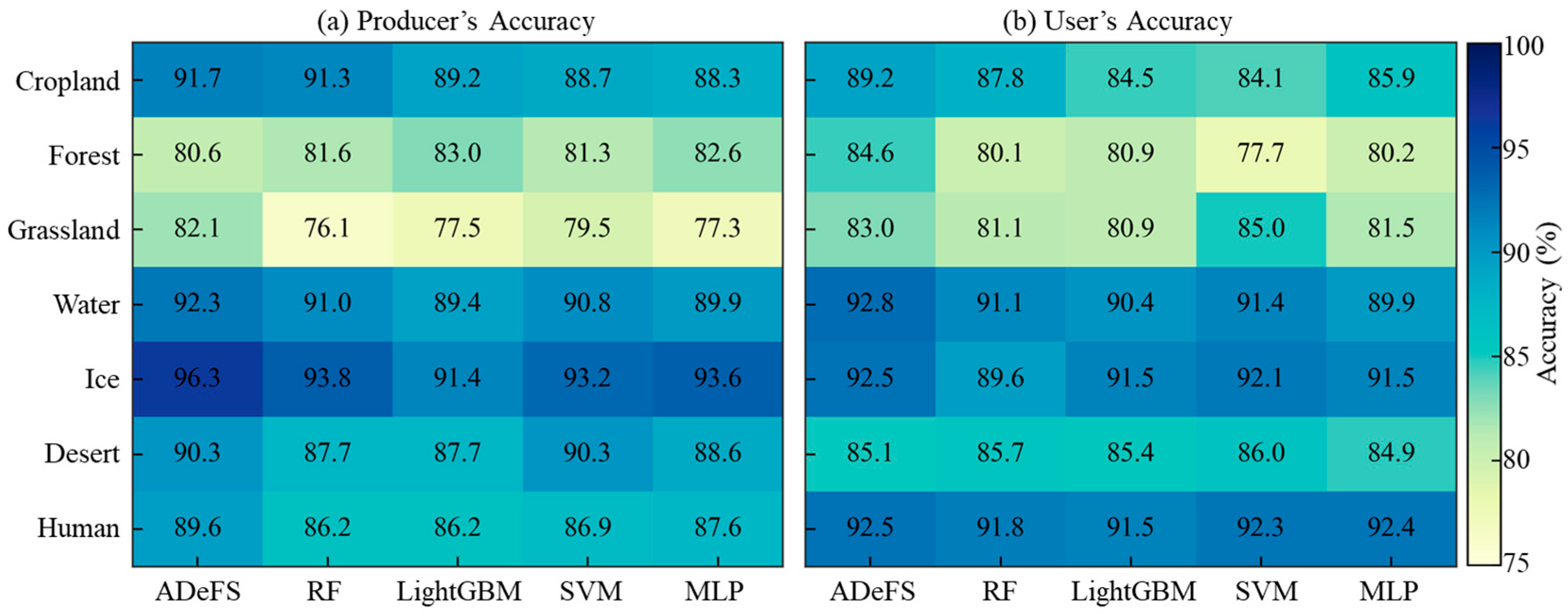
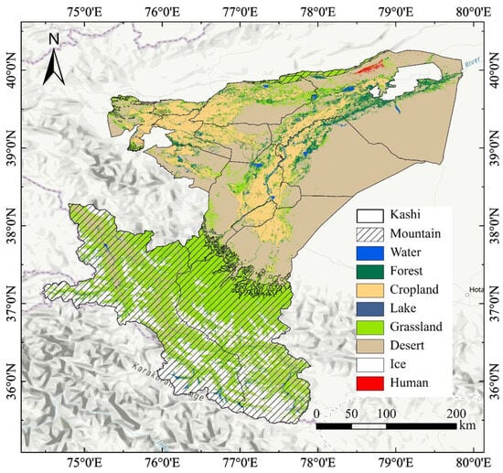
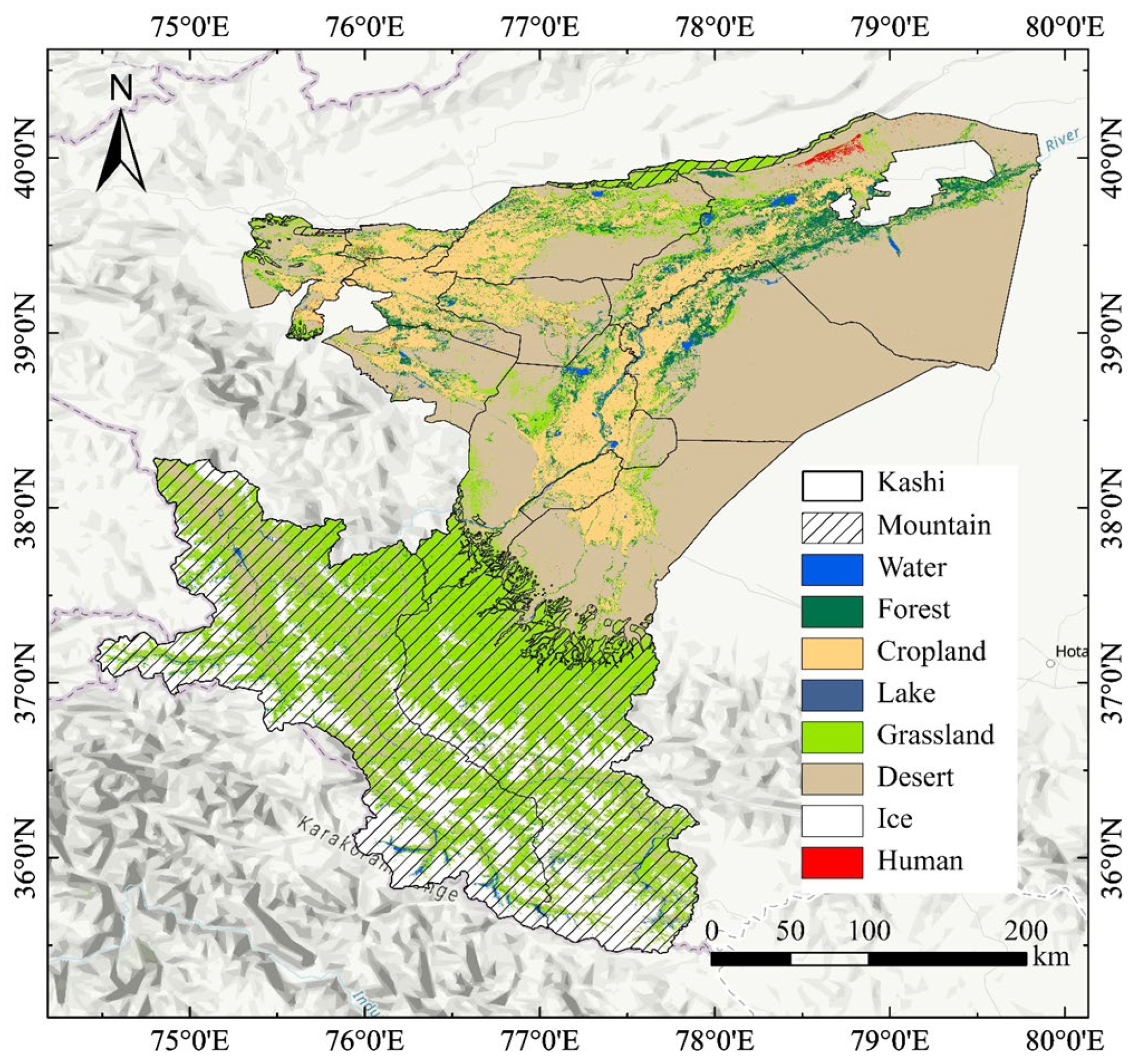
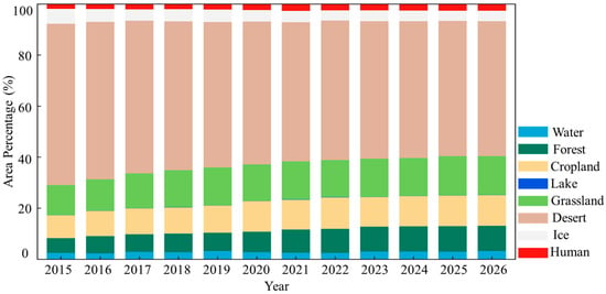
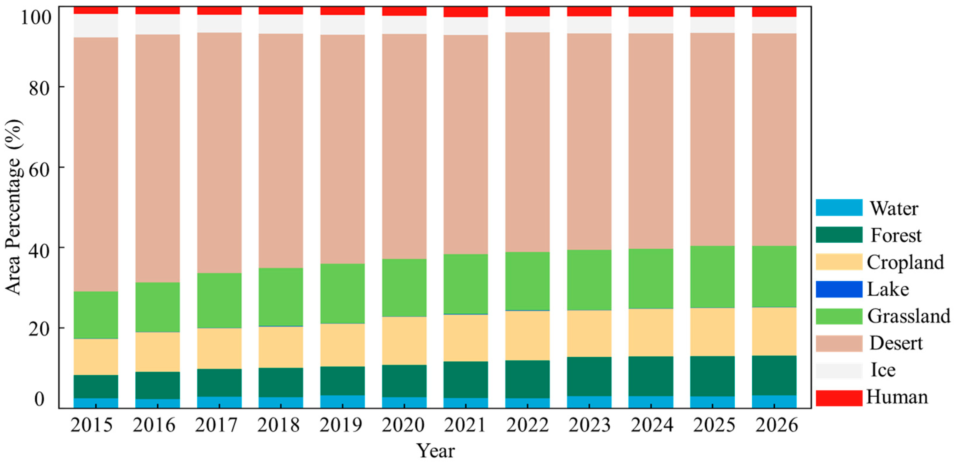
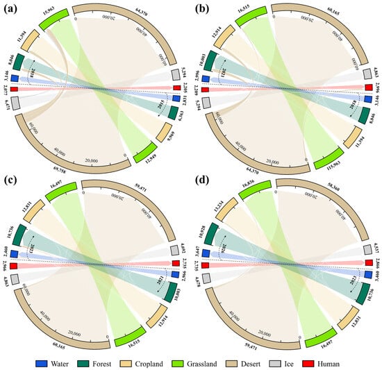
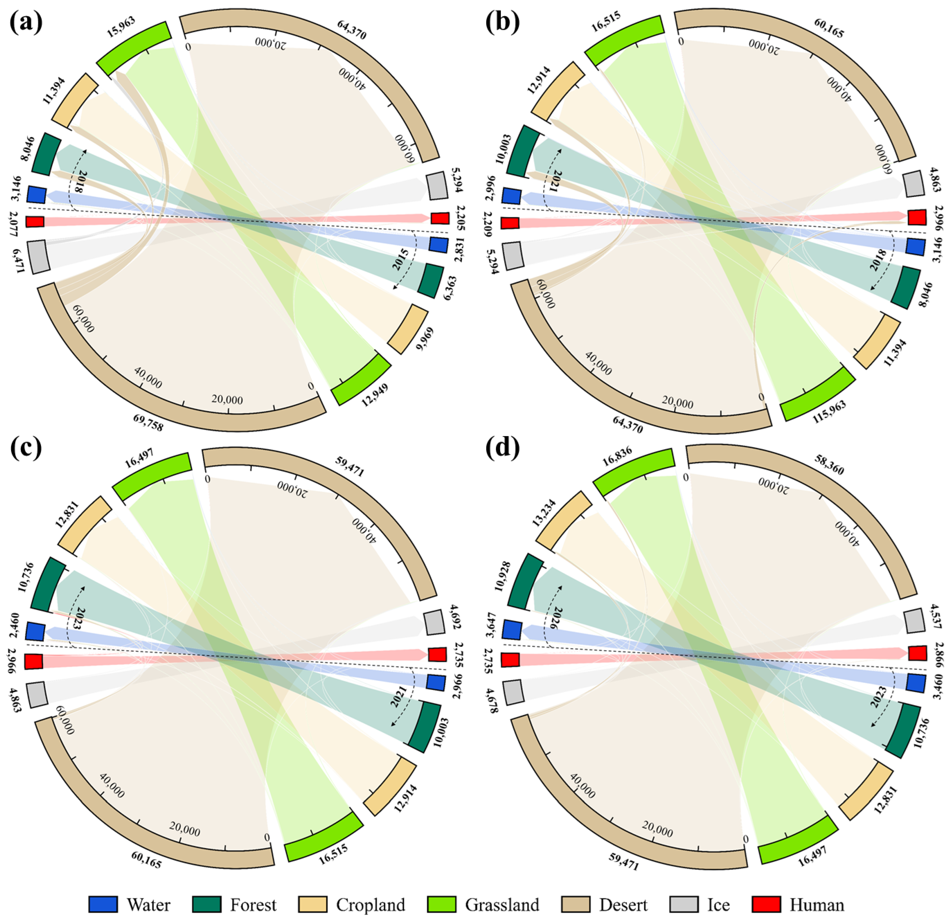
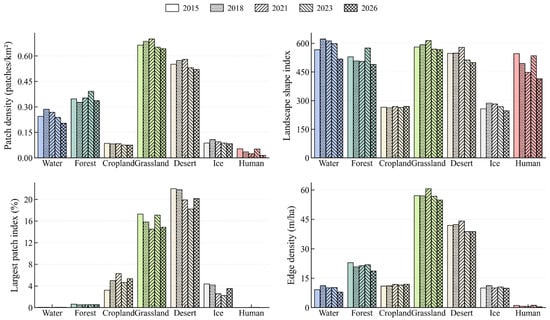
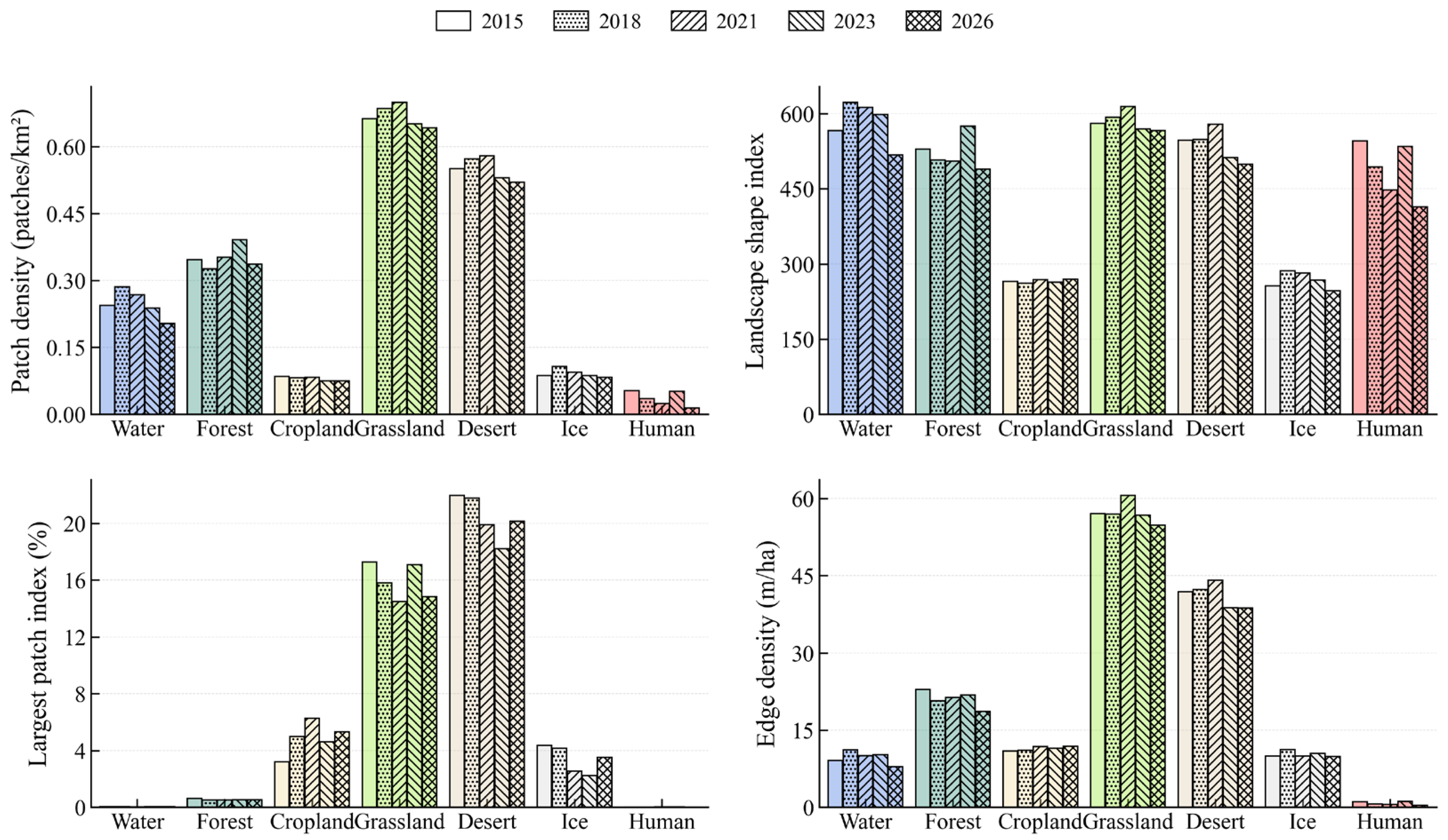

Disclaimer/Publisher’s Note: The statements, opinions and data contained in all publications are solely those of the individual author(s) and contributor(s) and not of MDPI and/or the editor(s). MDPI and/or the editor(s) disclaim responsibility for any injury to people or property resulting from any ideas, methods, instructions or products referred to in the content. |
© 2026 by the authors. Licensee MDPI, Basel, Switzerland. This article is an open access article distributed under the terms and conditions of the Creative Commons Attribution (CC BY) license.