


Abstract
Groundwater depth is a key control on soil salinization in arid irrigation districts, but seasonal groundwater depth thresholds for different salinization risks remain poorly constrained. Here, we examined the Yichang irrigation area of the Hetao Irrigation District using groundwater depth observations and 0–60 cm soil salinity samples collected before spring irrigation and during the crop-growing season. Indicator Kriging was used to map threshold-based probability zones for groundwater depth and soil salinity in the 0–60 cm root zone; soil salinity thresholds of 2 and 3 g kg−1 represented light-or-higher and moderate-or-higher salinization, respectively, and high-probability matching rates were used to identify the corresponding critical groundwater depths. Groundwater depth showed moderate spatial variability in both seasons, whereas soil salt content showed strong spatial variability. The critical groundwater depths for light and moderate salinization were 2.6 and 2.2 m before spring irrigation and 2.2 and 1.8 m during the growing season, respectively. Soil salt content in the 0–20, 20–40, 40–60 and 0–60 cm layers decreased with increasing groundwater depth, with the 0–60 cm layer well described by an exponential response function. These findings provide a spatially explicit basis for seasonal groundwater regulation, salinization risk zoning and field-scale water–salt management in arid irrigation districts.
1. Introduction
Soil salinization is a coupled process driven by climatic aridity, evaporative concentration, shallow groundwater, irrigation and drainage regimes, and land use [1,2,3,4,5,6,7,8]. Groundwater depth directly affects salt accumulation in the surface and cultivated soil layers by regulating capillary rise, salt transport into the root zone and post-irrigation leaching efficiency [6,8,9,10,11,12,13]. The effective control of groundwater depth is therefore a key approach for preventing and mitigating soil salinization in irrigated areas. Previous studies have examined this issue through soil salinity monitoring, remote-sensing inversion, numerical simulation, geostatistical mapping and risk assessment [9,12,14,15,16,17,18,19,20,21,22]. These studies provide technical support for quantifying the relationship between groundwater depth and soil salinity, but they also indicate that a single observation time or method is insufficient to characterize water–salt dynamics in irrigation districts. Integrated analyses combining field sampling, spatial interpolation, remote sensing and water–salt transport mechanisms are needed [12,16,22,23,24].
Remote sensing is an effective tool for monitoring soil salinization over large areas. Multispectral, hyperspectral and thermal imagery can identify salinization patterns from bare soil salt crust reflectance, vegetation salt stress responses, land surface temperature and salinity indices [14,15,16,17,18,19,20]. However, remote-sensing inversion mainly reflects surface or canopy responses and is affected by soil moisture, vegetation cover, vertical salt distribution and sampling scale. In irrigation districts, it therefore needs to be combined with ground measurements, groundwater depth observations and geostatistical models [9,16,18,19,20,21]. After salinity information has been obtained, the integration of hydrological and soil salinity data through statistical analysis and modelling provides an important basis for identifying groundwater depth thresholds and salinization risk zones [9,12,13,22].
Point-scale and regional water–salt transport models, based on Darcy’s law, the Richards equation, convection-dispersion theory, crop water consumption and salt stress effects, can simulate soil water and salt migration under different irrigation, drainage and groundwater depth conditions [23,24,25]. Models such as SaltMod, SWAP, SWAT-Salt and HYDRUS have been used to analyse water–salt balance, long-term salinity evolution and the effects of water-saving irrigation in irrigation districts [10,23,24,25]. These models represent physical mechanisms, but they generally require numerous parameters and boundary conditions. When combined with spatial sampling and geostatistical methods, they can better explain how regional groundwater depth control affects salt accumulation [12,23,24].
Classical statistics, geostatistics and geographic information systems are also widely used to investigate regional responses of soil salinization to groundwater depth [12,22,26,27,28,29,30,31]. Geostatistics is based on the regionalized variable theory and variograms, assuming that nearby samples tend to be more similar in attribute values. Semivariograms, Kriging, co-Kriging and indicator Kriging can therefore be used to reveal spatial structures in soil salinity and groundwater variables [26,29,30]. Indicator Kriging converts continuous variables into probabilities of exceeding predefined thresholds, making it suitable for mapping salinization risk zones, high-probability shallow groundwater zones and threshold-related uncertainty [27,28,31]. Previous work has shown that combining geostatistics with remote sensing, GIS and groundwater measurements helps identify the spatial differentiation and controlling factors of salinization risk [12,22,29,30].
Groundwater depth is therefore a central variable for managing soil salt accumulation in arid irrigation districts. Although remote sensing, geostatistical analysis and water–salt transport modelling have improved salinization risk assessment, most studies have treated soil salinity and groundwater depth as separate spatial variables. Less attention has been paid to whether their threshold-defined high-risk zones coincide in space. Critical groundwater depth is also often treated as a fixed value despite seasonal shifts in irrigation, evaporation, crop water use and salinization grade. Here, we used field observations from before spring irrigation and the growing season in the Yichang irrigation area to quantify the spatial response of soil salinization risk to groundwater depth using indicator Kriging. We further established layer-specific response functions between soil salt content and groundwater depth to support zoned salinization control and groundwater-level regulation. Unlike conventional point-scale regressions, the high-probability matching framework retains the spatial configuration of both variables and quantifies where threshold-defined shallow groundwater zones coincide with threshold-defined salinization risk zones. This spatial overlap provides a direct basis for seasonal risk zoning while avoiding the assumption that a single mean groundwater depth represents the entire irrigation area. This study does not claim to be the first demonstration of a groundwater depth–soil salinity relationship. Rather, the Yichang irrigation area is used as a case study to demonstrate a transferable workflow that links seasonal field observations, threshold-specific probability surfaces and spatial matching; the resulting numerical thresholds remain locally calibrated.
2. Materials and Methods
2.1. Regional Soil Salinization Survey
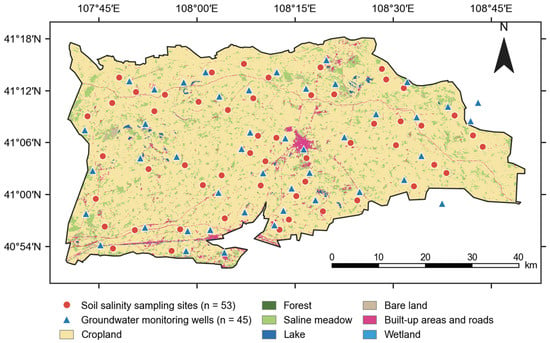
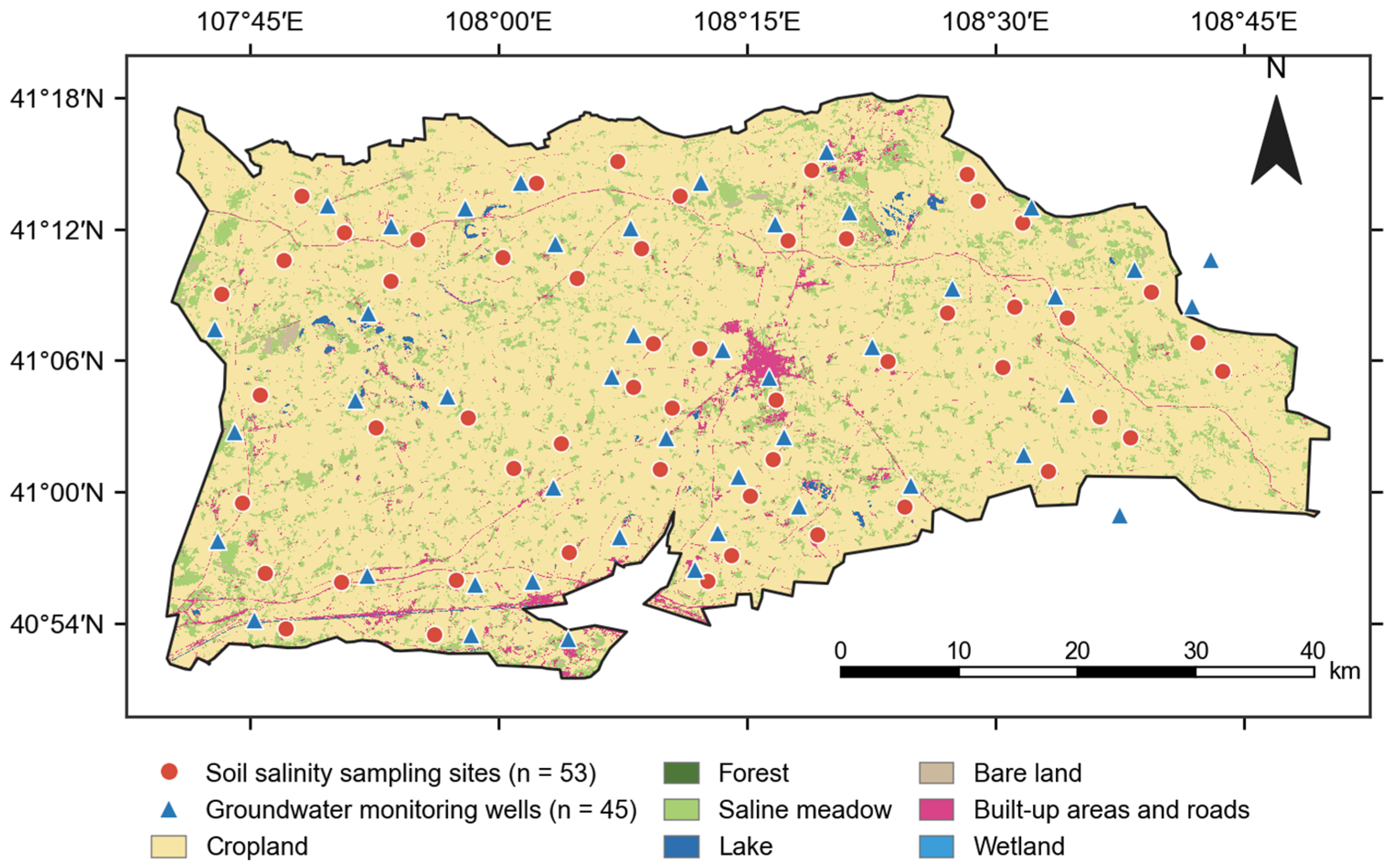
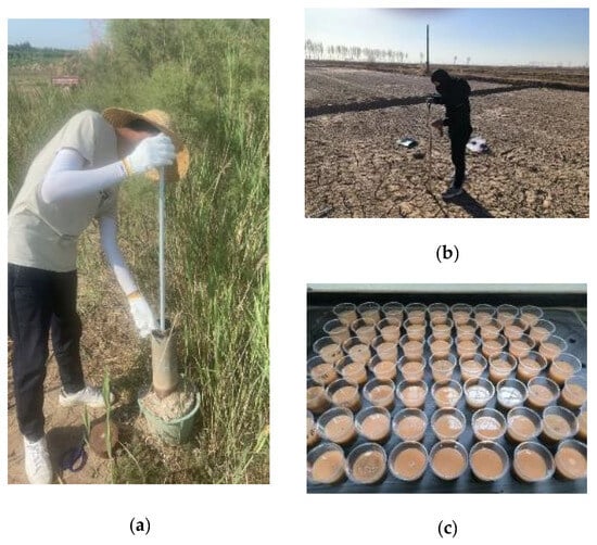
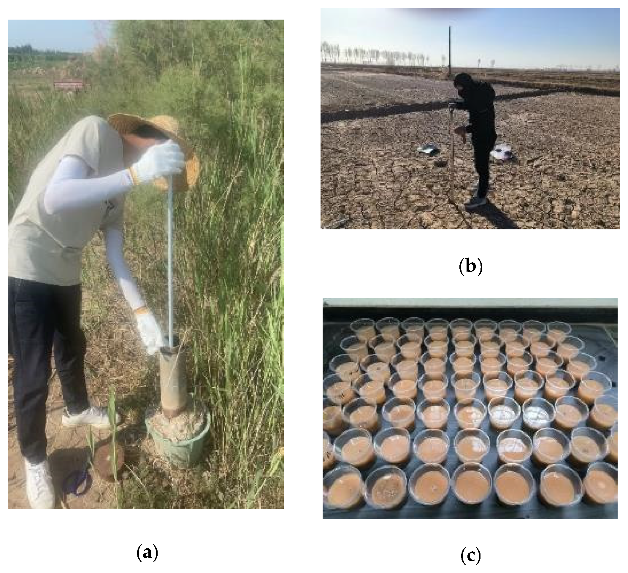
A regional survey was conducted in the Yichang irrigation area of the Hetao Irrigation District to examine how soil salinization responds to groundwater depth (Figure 1). The survey included groundwater depth observations and farmland soil sampling (Figure 2). To capture seasonal differences in the groundwater–salinity relationship, sampling was carried out before spring irrigation and during the crop-growing season. The irrigation area contained 45 groundwater observation wells, where groundwater depth was recorded every 5 d from before spring irrigation to the growing season. Field campaigns were conducted from 20 to 25 April 2020 and from 5 to 10 July 2020. Groundwater depth was measured in situ using a water level meter, and soil sampling sites were spatially distributed with reference to the groundwater observation network to support the comparison of their probability surfaces (Figure 1). In total, 53 soil salinity sampling sites were established. The final threshold-specific IK models used 45 complete records for each observation period; Figure 1 displays the full sampling network. At each site, samples were collected from 0–60 cm at 10 cm intervals, with three replicates per depth. Samples were weighed, oven-dried, ground, passed through a 2 mm sieve and extracted for soil salt content determination. For pointwise response analysis, each soil observation was linked to the contemporaneous groundwater depth measurement from its corresponding nearby observation well within the same campaign; groundwater values were not sampled from the IK rasters. The 0–20, 20–40 and 40–60 cm layer values describe depth-specific salinity, whereas the 0–60 cm value is their thickness-weighted mean. Because the three layers have equal thickness, S0−60 = (S0−20 + S20−40 + S40−60)/3. This integrated value represents overall cultivated/root zone salt exposure and is not an additional independent soil layer.
Figure 1.
Distribution of groundwater observation wells and soil salinity sampling sites.
Figure 2.
Groundwater depth observation, soil sampling and laboratory analysis. (a) Groundwater depth observation; (b) Field soil sampling; (c) Laboratory analysis of soil salinity.
2.2. Construction of the Salinization Risk–Groundwater Depth Relationship Based on Indicator Kriging
- (1)
- Method
Indicator Kriging (IK) is a non-parametric geostatistical method for estimating the probability that a variable exceeds a specified threshold at unsampled locations [26,27,28,31]. It is well suited to skewed distributions, threshold-defined events and spatial uncertainty because indicator transformation reduces the influence of extreme values on variogram estimation and yields probability-based risk maps [27,28]. Because the study concerns management-relevant exceedance events rather than unrestricted continuous-value prediction, IK was used to map groundwater depth and soil salinity probabilities on a common 0–1 scale. High-probability matching was then used to identify season-specific spatial correspondence between the two risk variables.
GS+ 7.0 was first used to determine variogram model parameters for soil salt content and groundwater depth under different thresholds. These parameters were then imported into ArcGIS 10.6 for IK interpolation, producing spatial probability maps of groundwater depth and root-zone soil salinity for the pre-spring irrigation and growing season periods. All IK rasters are probabilities on the same 0–1 scale. Additional min-max normalization or 95th/99th-percentile clamping was therefore not applied, because either operation would alter the probability interpretation of the threshold events. Comparisons were instead made directly on the common probability scale [22,26,27,28,29,30,31].
- (2)
- Threshold Selection and Indicator Kriging Model Construction
The key to IK is the rational selection of thresholds. Based on previous studies of shallow groundwater, salt accumulation and critical groundwater depth in arid and semi-arid irrigation districts [9,10,11,12,13,32,33], groundwater depth thresholds of 1.8, 2.2, 2.6 and 3.0 m were selected. When groundwater depth did not exceed a given threshold, the indicator value was set to 1; otherwise, it was set to 0. Soil salt content thresholds of 2 and 3 g kg−1 were selected to represent light-or-higher and moderate-or-higher salinization, respectively. These thresholds define regional soil salinization classes rather than crop-specific yield–loss limits. Common crops in the Hetao Irrigation District, including maize, sunflower and wheat, differ in salt tolerance and in sensitivity across growth stages; crop-specific risk interpretation therefore requires locally calibrated thresholds [5,8,34]. This threshold design converts continuous groundwater depth and soil salinity information into risk probabilities, facilitating the comparison of the spatial match between groundwater depth thresholds and salinization grades [13,22,28,31]. The workflow is transferable because the indicator definition, common probability scale and matching calculation are explicit; however, the numerical salinity and groundwater depth thresholds must be recalibrated for the crops, soils and hydrogeological setting of each application area.
Semivariogram parameters were used to characterize spatial dependence, and the C0/Sill ratio was interpreted as the relative contribution of short-range or random variability [26,29,30]. A probability value of 0.5 was used as the boundary between high- and low-probability zones. No unsupervised clustering algorithm was used; the terms high and low refer only to this probability classification. Probability maps were produced for groundwater depth and soil salinity thresholds, and the spatial matching rates between the two probability-zone types were calculated. This extends salinization risk identification from point-scale statistical relationships to regional spatial response relationships [27,28,31]. Predictive performance was evaluated by the leave-one-out cross-validation of each threshold-specific IK model. Each observation was omitted in turn, and its indicator probability was predicted from the remaining observations. The 12 final IK models each contained 45 complete records for cross-validation.
Here, n is the number of cross-validation observations (n = 45), Ii is the observed binary indicator (Ii ∈ {0,1}), pi is the leave-one-out predicted probability (pi ∈ [0,1]), ei = pi − Ii, and zi = ei/si, where si is the Kriging standard error. The validation metrics were calculated as follows:
For a binary indicator, the mean CRPS is equivalent to the Brier score. Values of ME and mean standardized error near zero indicate low average bias, whereas an RMS standardized error near one indicates that the kriging standard errors are consistent with the observed prediction errors.
3. Results
3.1. Spatial Probability Characteristics of Groundwater Depth
3.1.1. Descriptive Statistics of Groundwater Depth
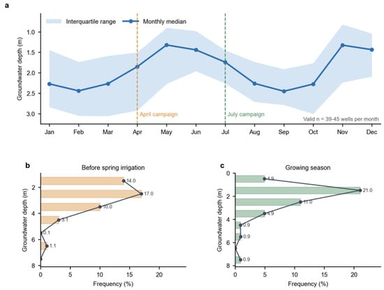
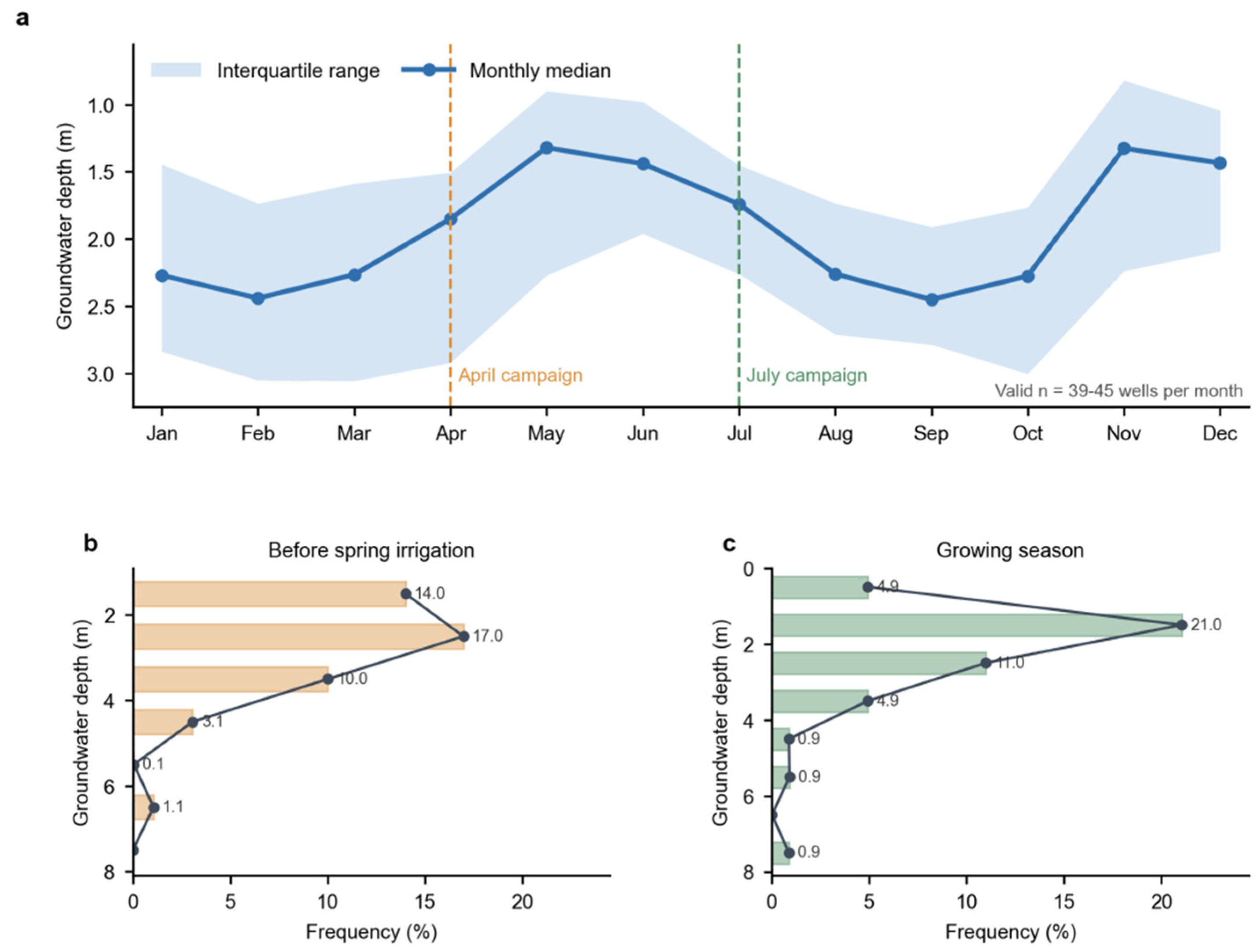
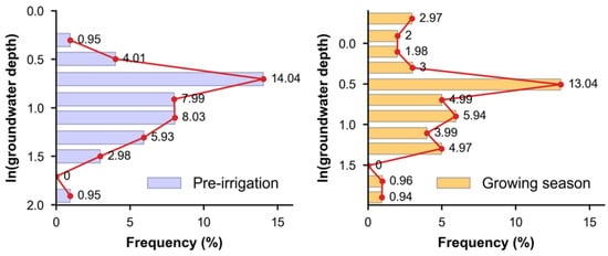
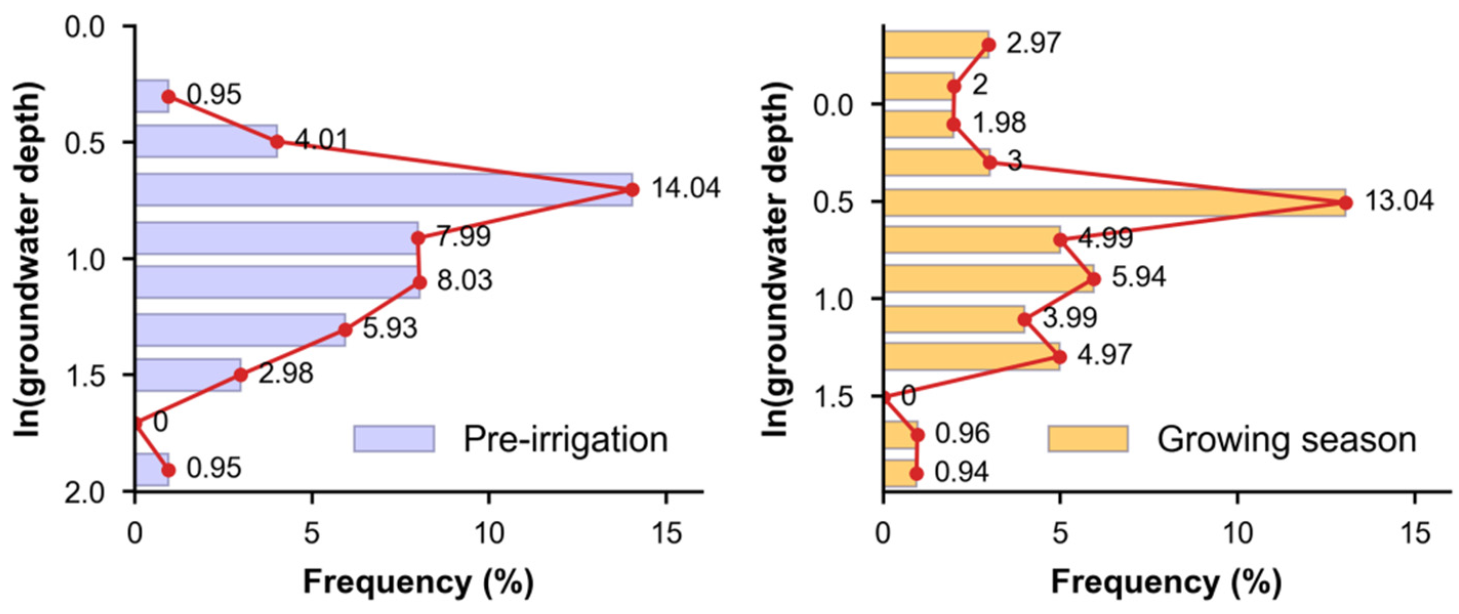
Groundwater depth differed between the two sampling periods (Table 1). Monthly monitoring further showed a clear seasonal cycle (Figure 3a): across the observation well network, the monthly median depth ranged from 1.32 m in May to 2.45 m in September. The April and July medians were 1.85 and 1.74 m, respectively, and valid monthly observations ranged from 39 to 45 wells. Before spring irrigation, groundwater depth ranged from 1.23 to 6.43 m with a mean of 2.83 m. During the growing season, it ranged from 0.54 to 8.56 m with a mean of 2.45 m. The standard deviations were 0.96 and 1.26 m, and the coefficients of variation were 0.34 and 0.64 before spring irrigation and during the growing season, respectively. Both coefficients indicate moderate variability, but the larger value during the growing season suggests stronger spatial fluctuation, probably reflecting irrigation, cultivation and other management or environmental influences. Before spring irrigation, groundwater depth was relatively more stable, partly because residual autumn irrigation water gradually replenished groundwater. Figure 3 shows the frequency distributions of groundwater depth before spring irrigation and during the growing season. Before spring irrigation, the 2–3-m interval had the highest frequency (16.98%), followed by the 0–1-m interval (14.01%); frequency decreased as depth increased. During the growing season, the 1–2-m interval had the highest frequency (21.04%), whereas the 2–3-m and 0–1-m intervals accounted for 10.99% and 4.92%, respectively. Frequencies again declined with increasing depth. Both periods showed positively skewed distributions, with extreme values in shallow-depth intervals. Therefore, groundwater depth frequencies were logarithmically transformed (Figure 4). Although the transformed frequencies approached a normal distribution, outliers remained, indicating that groundwater depth contained extreme values under different data-processing methods.
Table 1.
Statistical characteristics of groundwater depth before spring irrigation and during the growing season in 2020 (n = 45 observation wells).
Figure 3.
Seasonal groundwater depth variation and campaign-specific distributions in 2020. (a) Monthly median and interquartile range across the observation well network; (b) frequency distribution before spring irrigation; and (c) frequency distribution during the growing season. Non-positive monthly values were omitted from the descriptive summaries because they fell outside the field-observed depth range; valid n ranged from 39 to 45 wells per month.
Figure 4.
Frequency distribution of logarithmically transformed groundwater depth.
3.1.2. Construction of Indicator Variogram Models for Groundwater Depth
The variogram model was first selected. Compared with exponential, Gaussian and linear models, the spherical model has broader applicability and a clear range of spatial correlation. It was therefore used to obtain variogram parameters for different groundwater depth thresholds before spring irrigation and during the growing season. The groundwater depth thresholds were 1.8, 2.2, 2.6 and 3.0 m. The theoretical indicator variogram models are shown in Table 2. Nugget values ranged from 0.046 to 0.076, and sill values ranged from 0.092 to 0.156. Both increased with the threshold, indicating that spatial variability strengthened as groundwater depth increased. Nugget values during the growing season were generally higher than those before spring irrigation, indicating greater spatial variability in groundwater depth. C0/Sill represents spatial correlation: C0/Sill < 0.25 indicates strong large-scale spatial correlation, 0.25 ≤ C0/Sill < 0.75 indicates moderate spatial correlation, and C0/Sill ≥ 0.75 indicates weak spatial autocorrelation, with most variability arising from small-scale variation or measurement error. For all thresholds in both periods, C0/Sill ranged from 43.22% to 53.54%, indicating moderate spatial autocorrelation. The higher C0/Sill during the growing season suggests a larger random component. The A0 values were similar between the two periods, indicating no substantial seasonal difference in the spatial correlation range of groundwater depth. Leave-one-out cross-validation showed threshold-dependent predictive performance across the eight groundwater depth indicator models, with ME ranging from −0.689 to 0.647, RMSE from 0.419 to 0.785, and binary CRPS from 0.176 to 0.616. For the thresholds used in the final management interpretation, the pre-spring irrigation 2.2- and 2.6-m models had ME values of 0.210 and −0.106, RMSE values of 0.590 and 0.547, and CRPS values of 0.348 and 0.299, respectively. The growing season 1.8- and 2.2-m models had ME values of −0.005 and −0.015, RMSE values of 0.574 and 0.419, and CRPS values of 0.330 and 0.176, respectively. The larger errors for some thresholds indicate that the probability maps are more appropriate for regional risk zoning than for precise prediction in individual fields.
Table 2.
Theoretical indicator variogram models for groundwater depth before spring irrigation and during the growing season in 2020.
3.1.3. Spatial Probability Distribution of Groundwater Depth Before Spring Irrigation
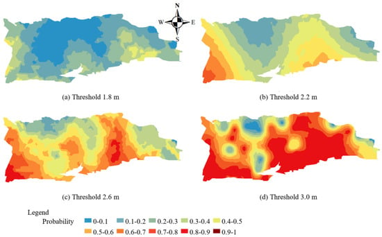
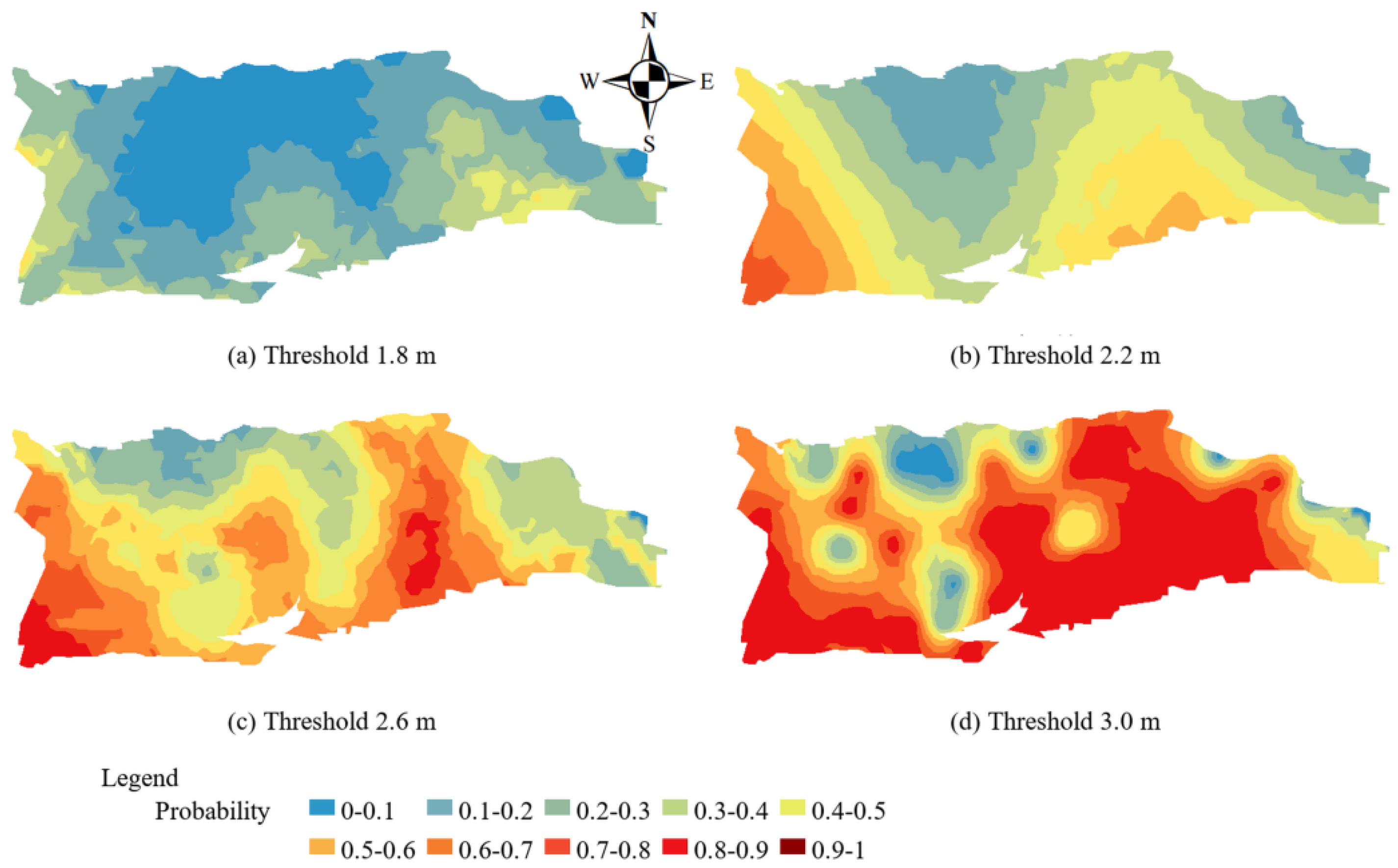
The constructed indicator Kriging models were used to predict spatial probability distributions for different groundwater depth thresholds before spring irrigation (Figure 5). In the legend, blue denotes low-probability zones, and red denotes high-probability zones. At a threshold of 1.8 m, most of the area was in the low-probability zone, with only some high-probability areas along the western and eastern margins, indicating a low probability of groundwater depth being shallower than 1.8 m across most of the region. At 2.2 m, high-probability zones increased markedly and displayed a banded pattern, mainly in the eastern and central-eastern areas. At 2.6 m, red areas expanded substantially, and most of the region became high probability, with low-probability zones remaining only in the northern and eastern margins. At 3.0 m, high-probability areas expanded further, leaving only scattered local low-probability zones.
Figure 5.
Spatial probability distribution of groundwater depth before spring irrigation in 2020.
A probability value of 0.5 was used as the boundary between high- and low-probability zones. The proportions and areas of the two probability classes under each threshold are summarized in Table 3. As the groundwater depth threshold increased, the proportion of high-probability zones increased from 16% to 83%, and their area increased from 523.52 to 2715.76 km2. This pattern is consistent with the frequency distribution before spring irrigation in Table 1, where the 2–3-m groundwater depth interval had the highest frequency.
Table 3.
Area proportions of groundwater depth probability zones under different thresholds before spring irrigation in 2020.
3.1.4. Spatial Probability Distribution of Groundwater Depth During the Growing Season
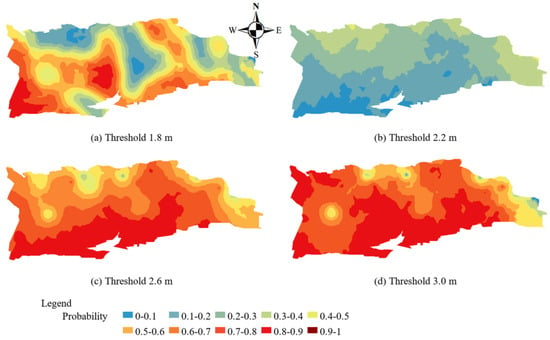
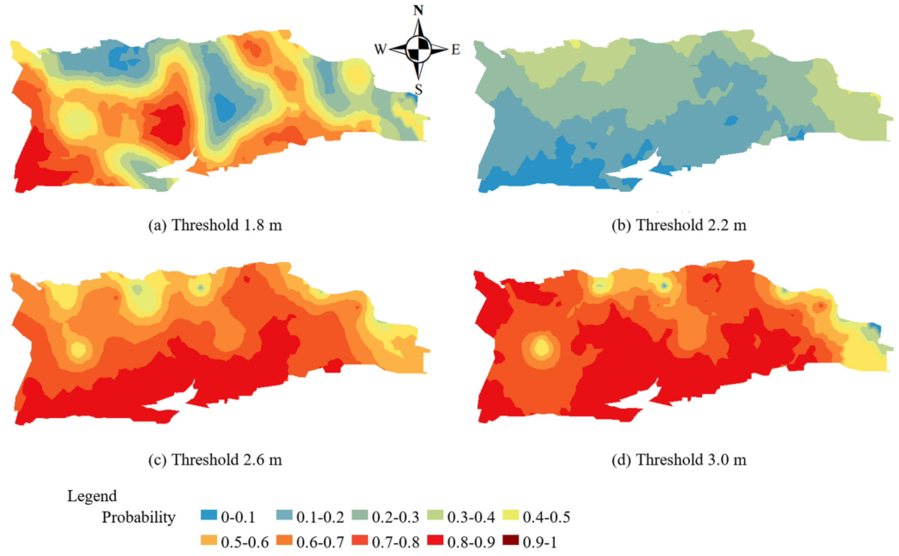
Using the variogram parameters in Table 2, IK was applied to predict the spatial probability distributions of groundwater depth during the growing season (Figure 6), and the proportions of high- and low-probability zones were calculated (Table 4). At a threshold of 1.8 m, most of the area was classified as low probability, although probabilities in the north were higher than those in the south; the high-probability area accounted for 16%. At 2.2 m, high-probability zones increased significantly, mainly in the western, central and central-eastern parts of the irrigation area, accounting for 36% of the total area. At 2.6 m, red areas expanded further, with higher probabilities mainly in the south; the high-probability area accounted for 74%. At 3.0 m, 82% of the irrigation area was high-probability, while low-probability zones were concentrated in northern and eastern piedmont areas. Compared with the pre-spring irrigation period (Figure 5), groundwater depth became shallower during the growing season because of irrigation. Most areas had groundwater depths of 1–2 m, so high-probability areas increased markedly under larger thresholds.
Figure 6.
Spatial probability distribution of groundwater depth during the growing season in 2020.
Table 4.
Area proportions of groundwater depth probability zones under different thresholds during the growing season in 2020.
3.2. Spatial Probability Characteristics of Soil Salt Content
3.2.1. Descriptive Statistics of Soil Salt Content
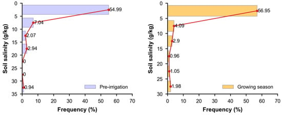
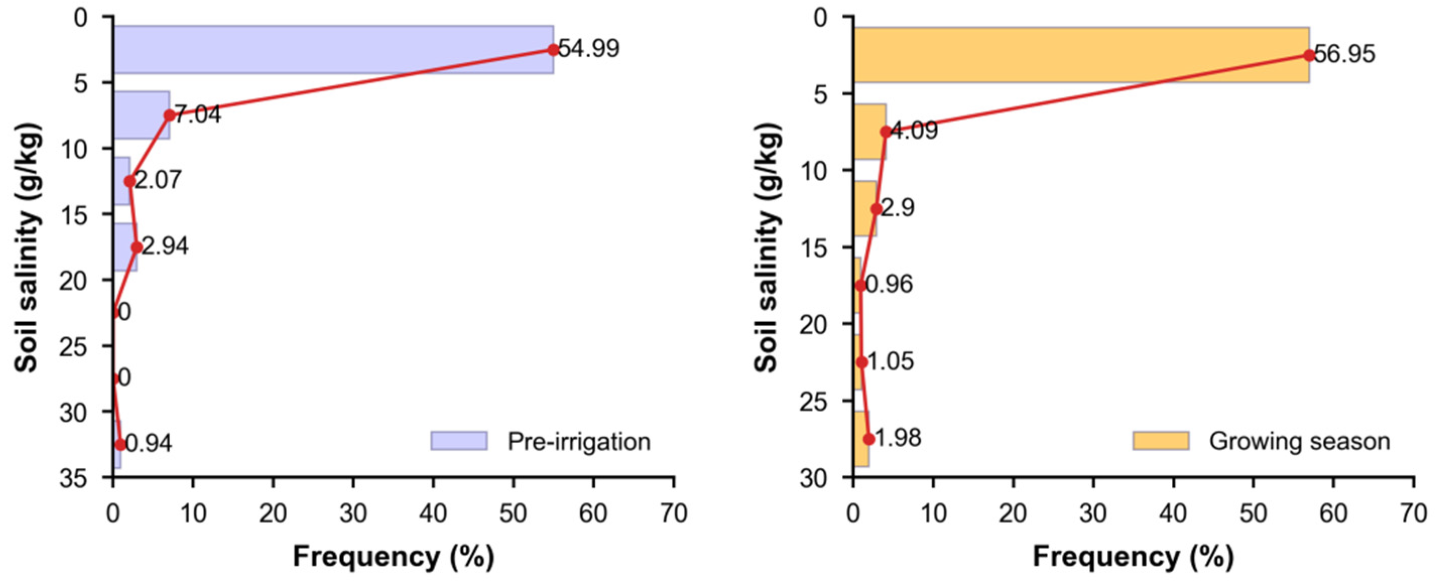
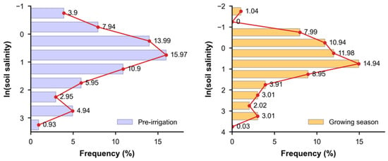
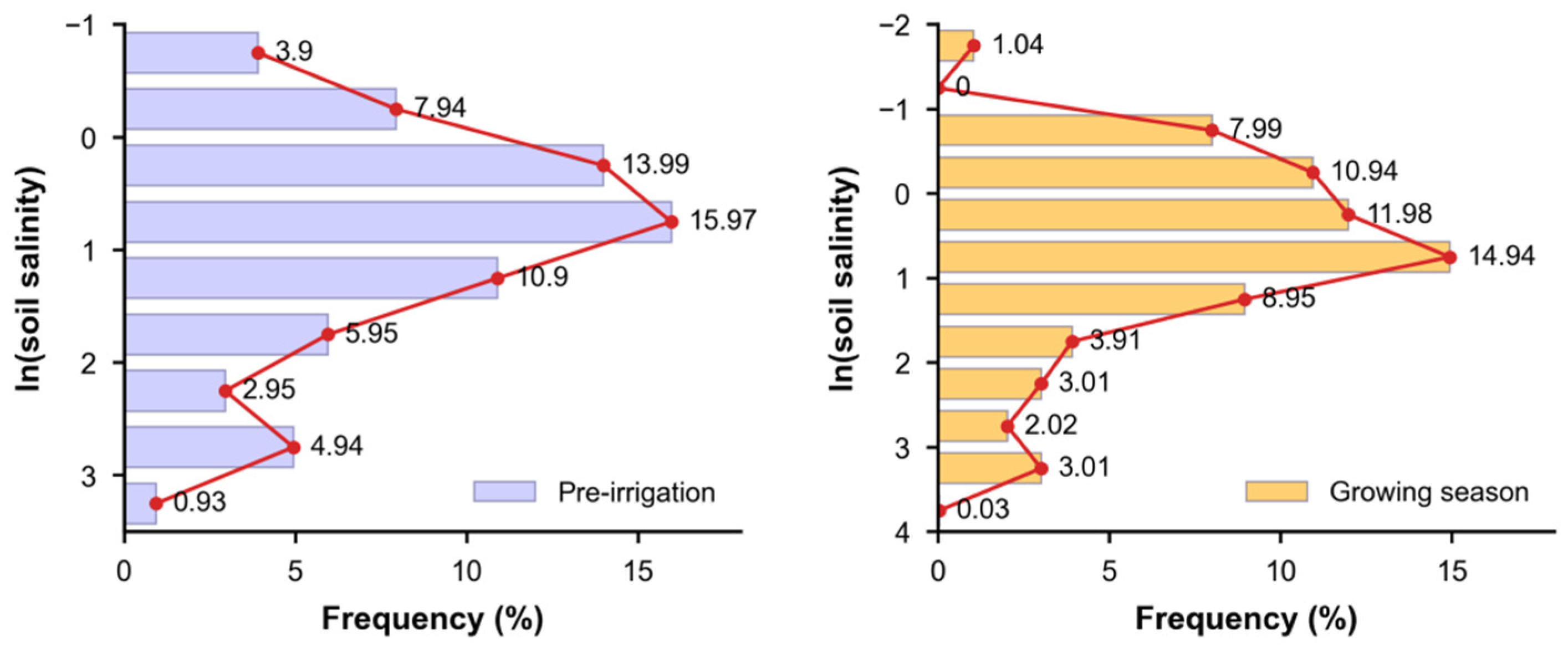
Soil salt content also varied strongly between sampling sites (Table 5). Before spring irrigation, it ranged from 0.46 to 33.56 g kg−1 with a mean of 3.87 g kg−1. During the growing season, it ranged from 0.21 to 29.40 g kg−1 with a mean of 3.54 g kg−1. The slightly higher mean before spring irrigation indicates stronger spring salt return, although both periods showed broad distributions. The coefficients of variation were 1.42 before spring irrigation and 1.63 during the growing season, indicating strong spatial variability in both periods and greater heterogeneity during the growing season. Figure 7 shows the frequency distributions of soil salt content before spring irrigation and during the growing season. In both periods, the 0–5 g kg−1 interval had the highest frequency, accounting for 54.99% and 56.95%, respectively. Frequency declined as salt content increased, and the distributions were positively skewed, similar to groundwater depth. After logarithmic transformation, the frequency distribution approached normality (Figure 8), but outliers remained. Given the data structure, IK, which is better suited for skewed data, was used to analyse spatial probability distributions.
Table 5.
Statistical characteristics of soil salt content before spring irrigation and during the growing season in 2020.
Figure 7.
Frequency distribution of soil salt content.
Figure 8.
Frequency distribution of logarithmically transformed soil salt content.
3.2.2. Construction of Indicator Variogram Models for Soil Salt Content
Following the groundwater depth modelling procedure, the spherical model was also used to obtain variogram parameters for soil salt content under different thresholds before spring irrigation and during the growing season. The resulting indicator variogram parameters are shown in Table 6. Nugget values ranged from 0.048 to 0.066, sill values from 0.105 to 0.134, ranges from 7.07 to 7.14 km, and C0/Sill from 35.82% to 62.86%, indicating moderate spatial autocorrelation. Before spring irrigation, C0/Sill was 61.29% at the 2 g kg−1 threshold, close to 75%, indicating that random small-scale variation or measurement error contributed substantially to total variation and that spatial indication was relatively weak. At the 3 g kg−1 threshold, C0/Sill was 41.88%, indicating stronger spatial dependence. During the growing season, C0/Sill was 35.82% at the 2 g kg−1 threshold, suggesting that spatial variation in soil salt content was more strongly controlled by spatial autocorrelation. At the 3 g kg−1 threshold, C0/Sill increased to 62.86%, indicating weaker spatial dependence. The stronger spatial dependence during the growing season under the low-salinity threshold is related to irrigation, rainfall and farming practices. The leave-one-out cross-validation of the four soil salinity indicator models yielded ME values from −0.003 to 0.023, RMSE values from 0.395 to 0.517, and binary CRPS values from 0.156 to 0.268. Root-mean-square standardized errors ranged from 0.949 to 1.047, indicating broadly consistent uncertainty scaling, although the threshold-specific RMSE values require the probability boundaries to be interpreted as regional risk zones rather than exact field boundaries.
Table 6.
Theoretical indicator variogram models for soil salt content before spring irrigation and during the growing season in 2020.
3.2.3. Soil Salinization Risk Before Spring Irrigation
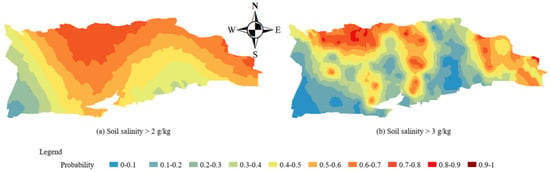
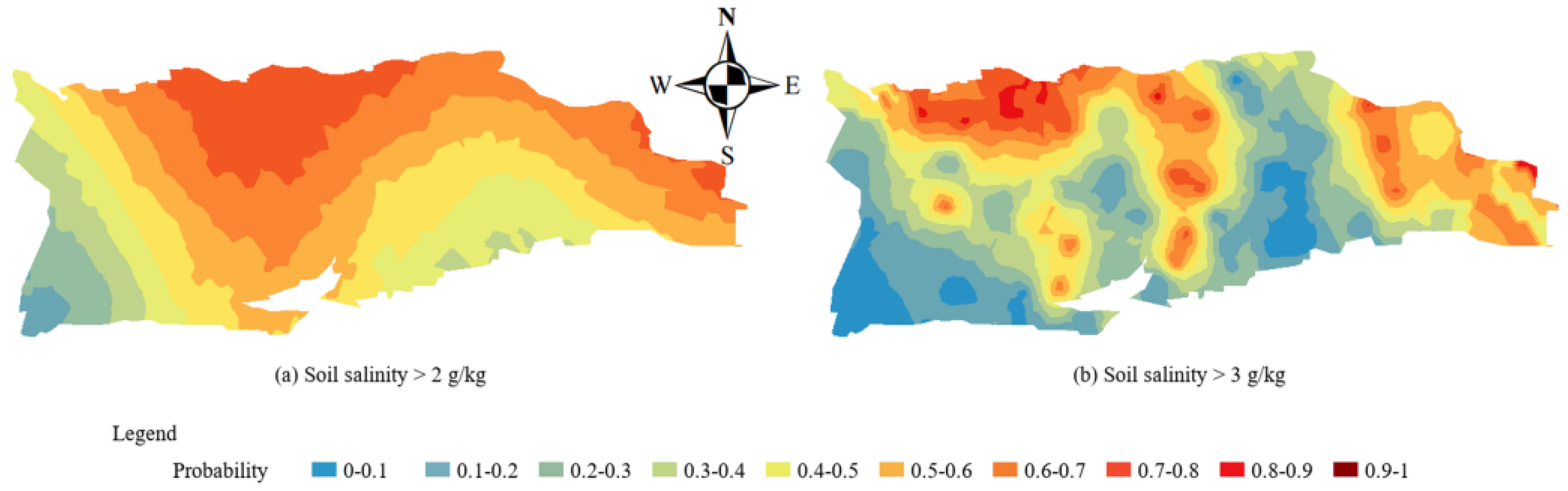
Using the variogram parameters for soil salt content thresholds of 2 and 3 g kg−1 in Table 6, IK was applied to predict spatial probability distributions (Figure 9), and the proportions of high- and low-risk zones before spring irrigation were calculated (Table 7). At the 2 g kg−1 threshold, 76% of the area was high-risk and 24% was low-risk. High-risk zones were concentrated mainly in the central-northern area, with probabilities increasing northward. At the 3 g kg−1 threshold, 46% of the area was high-risk and 54% was low-risk; high-risk zones were mainly located in the northern and eastern areas. Because elevation decreases from southwest to northeast, lower-lying areas have shallower groundwater and a higher probability of salinization risk.
Figure 9.
Spatial probability distribution of soil salt content under different thresholds before spring irrigation in 2020.
Table 7.
Area proportions of soil salinity risk zones under different thresholds before spring irrigation in 2020.
3.2.4. Soil Salinization Risk During the Growing Season
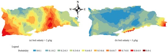
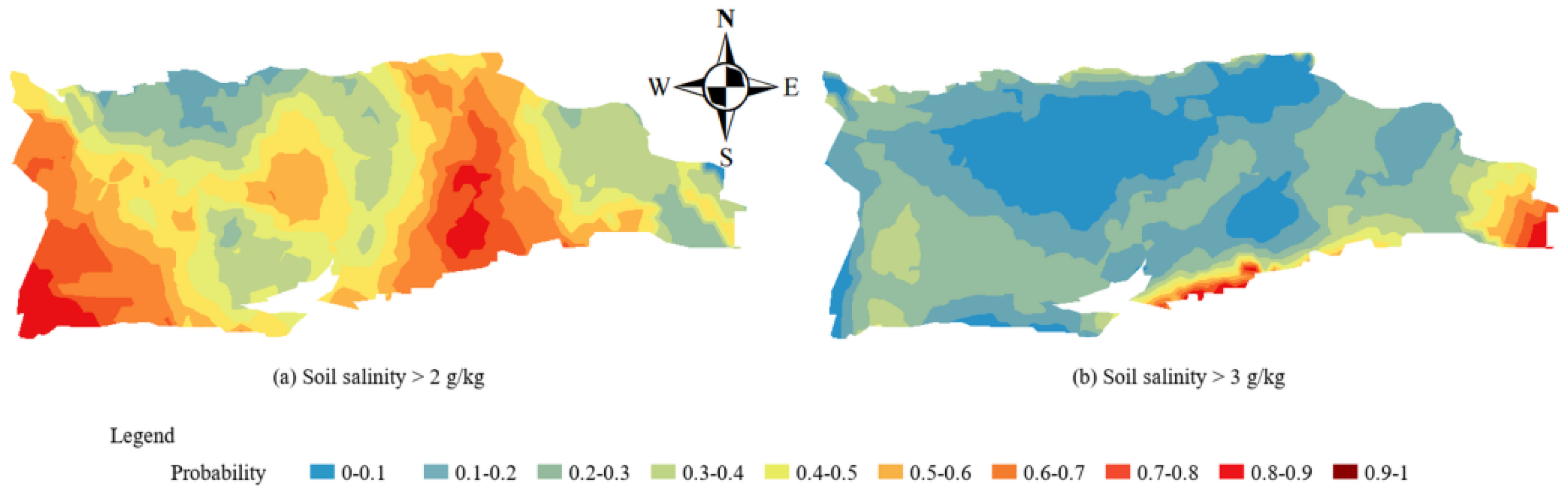
The spatial probabilities of soil salinization under light and moderate soil salt content thresholds during the growing season are shown in Figure 10, and the proportions of high- and low-risk zones are summarized in Table 8. When the threshold was 2 g kg−1, high-risk zones accounted for 84% of the irrigation area and were mainly distributed in the western, central and central-eastern areas. When the threshold was 3 g kg−1, the high-risk area decreased markedly to 16%, mainly along the southern and eastern margins. Comparing the two seasons, the high-risk area at the 2 g kg−1 threshold was larger during the growing season than before spring irrigation, indicating a higher risk of light salinization during the growing season. At the 3 g kg−1 threshold, the high-risk area was larger before spring irrigation, indicating a higher risk of moderate salinization in spring. Much of the high-risk area before spring irrigation shifted to low risk during the growing season, indicating a transition from moderate to light salinization. This occurred because irrigation and farming practices leached surface and shallow soil salts into deeper layers or groundwater, reducing salt content in the cultivated layer. Before spring irrigation, evaporation promoted stronger salt return, causing salts from deeper soil and groundwater to accumulate near the surface and increasing the risk of moderate salinization.
Figure 10.
Spatial probability distribution of soil salt content under different thresholds during the growing season in 2020.
Table 8.
Area proportions of soil salinity risk zones under different thresholds during the growing season in 2020.
Complete threshold-specific leave-one-out cross-validation results for all 12 final IK models are summarized in Table 9. Several groundwater depth thresholds showed appreciable bias or RMS standardized errors above one, confirming that the resulting maps should be interpreted as regional probability zones rather than precise field-scale predictions.
Table 9.
Leave-one-out cross-validation metrics for the 12 threshold-specific indicator Kriging models (n = 45 for each model).
4. Discussion
4.1. Spatiotemporal Groundwater Depth Variation and the Distribution of Salinized Soil Types
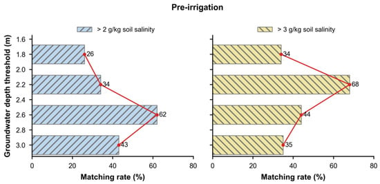
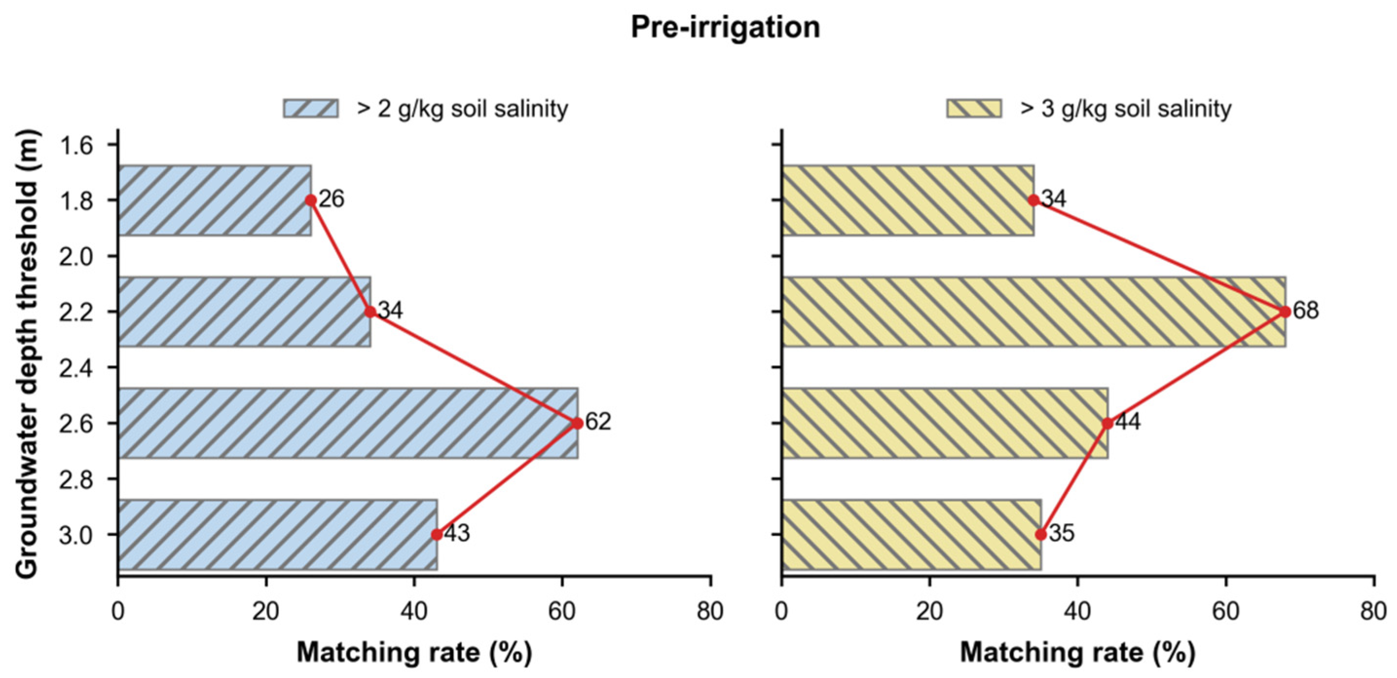
The spatial probability distributions under different groundwater depth thresholds were compared with those under different soil salt content thresholds, and high-probability matching rates were used to determine groundwater depth thresholds for controlling different salinization risk grades. Comparing Figure 5 with Figure 9 shows that the high-probability area under the 2.6-m groundwater depth threshold overlapped strongly with the high-risk area under the 2 g kg−1 soil salt content threshold. The high-probability area under the 2.2-m groundwater depth threshold also matched the high-risk area under the 3 g kg−1 threshold. Further matching analysis (Figure 11) showed that, when the soil salt content threshold was 2 g kg−1, the matching rates with groundwater depth thresholds of 1.8, 2.2, 2.6 and 3.0 m were 26%, 34%, 62% and 43%, respectively. The highest match occurred at 2.6 m, indicating that the critical groundwater depth for light salinization before spring irrigation was 2.6 m. When the soil salt content threshold was 3 g kg−1, the matching rates were 34%, 68%, 44% and 35%, respectively, with the highest match at 2.2 m. Therefore, the critical groundwater depth for moderate salinization before spring irrigation was 2.2 m.
Figure 11.
Matching rates between soil salt content and groundwater depth probability zones under different thresholds before spring irrigation in 2020.
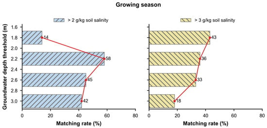
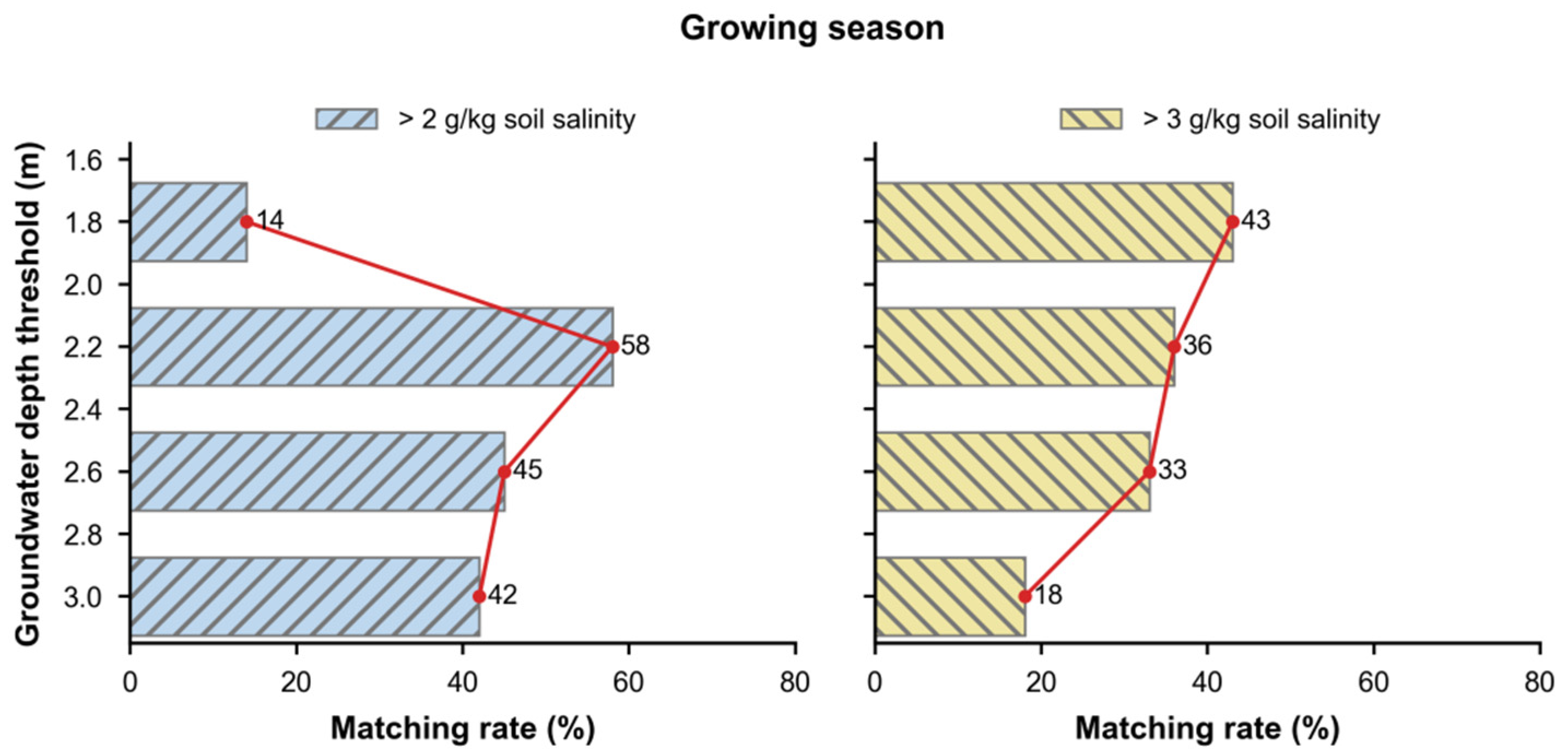
For the growing season, spatial probability distributions under soil salt content thresholds of 2 and 3 g kg−1 were compared with those under groundwater depth thresholds of 1.8, 2.2, 2.6 and 3.0 m. Comparing Figure 4 with Figure 10 shows that the high-probability area under the 2.2-m groundwater depth threshold overlapped strongly with the high-risk area under the 2 g kg−1 salt content threshold. The high-probability area under the 1.8-m threshold also showed a high matching rate with the high-risk area under the 3 g kg−1 threshold. Further matching analysis (Figure 12) showed that, when the soil salt content threshold was 2 g kg−1, the matching rates with groundwater depth thresholds of 1.8, 2.2, 2.6 and 3.0 m were 14%, 58%, 45% and 42%, respectively. The highest matching rate was 58% at 2.2 m, so 2.2 m can be regarded as the critical threshold for controlling light salinization during the growing season. When the soil salt content threshold was 3 g kg−1, the matching rates were 43%, 36%, 33% and 18%, respectively. The highest match occurred at 1.8 m, indicating that the critical groundwater depth for moderate salinization during the growing season was 1.8 m.
Figure 12.
Matching rates between soil salt content and groundwater depth probability zones under different thresholds during the growing season in 2020.
The seasonal groundwater depth thresholds identified here show that critical groundwater depth should not be treated as a single fixed value. In the Yichang irrigation area, the thresholds for light and moderate salinization were 2.6 and 2.2 m before spring irrigation, but they shifted to 2.2 and 1.8 m during the growing season. This seasonal difference is consistent with changes in water–salt transport direction, irrigation leaching and crop growth stage [6,10,11,12,13,23,24,32,33]. Before spring irrigation, stronger evaporation and limited crop cover promote upward salt transport from shallow groundwater. During the growing season, irrigation leaching, crop water use and root zone redistribution jointly reshape soil salinity. Separating critical groundwater depth by season and salinization grade therefore provides a more realistic basis for arid-district water–salt management.
Mechanistically, the threshold difference reflects a seasonal shift among three processes: evaporative salt return, irrigation leaching and crop water consumption. Before spring irrigation, a larger bare-soil fraction strengthens upward salt movement and makes shallow-groundwater areas more prone to salt accumulation in surface and near-surface layers. During the growing season, irrigation can leach salts downward, while crop water uptake modifies root-zone moisture gradients and redistributes salts among soil layers [6,10,12,32,33]. At the same time, expanding root systems increase water extraction from the cultivated layer, and canopy development shades the soil surface and suppresses bare-soil evaporation. These processes weaken upward liquid flux and evaporative salt concentration near the surface. Together with irrigation leaching, they help explain why a shallower critical groundwater depth can occur during the growing season without producing the same degree of topsoil salt accumulation observed before spring irrigation.
The high-probability matching approach provides information that cannot be obtained from mean groundwater depth alone. It identifies where shallow-groundwater probability zones coincide with salinization risk zones, thereby linking groundwater regulation to spatially explicit risk control. The results suggest that management should avoid applying a single groundwater-control level across the whole irrigation area. Instead, seasonal thresholds should be defined separately for preventing light salinization and mitigating moderate salinization [13,22,28,31]. The general contribution is the reproducible probability-matching workflow rather than a universal groundwater depth value. Its sequence can be applied elsewhere, but the event thresholds and variogram models require local calibration before regional transfer.
4.2. Quantitative Relationship Between Groundwater Depth and Soil Salinity
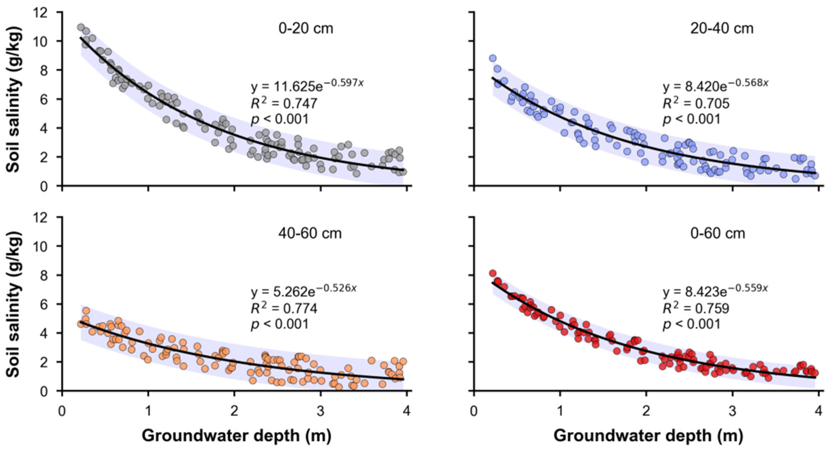
To determine the response of soil salinity in different layers to groundwater depth, soil observations from 53 sampling sites were linked to contemporaneous measurements from their corresponding nearby wells within each campaign. The regressions therefore used field/well pairs at the sampling-unit scale rather than groundwater values extracted from the IK rasters. Records flagged as incomplete or as outliers during the original quality control procedure were excluded before fitting. Layer-specific scatterplots and fitted curves are presented together in Figure 13. In all four soil layers, soil salt content decreased as groundwater depth increased. The scatter-plot patterns were consistent with exponential attenuation relationships, so exponential functions were used to describe the responses.
Figure 13.
Relationships between groundwater depth and soil salt content in the 0–20, 20–40, 40–60 and 0–60 cm soil layers. Solid curves show exponential fits, shaded regions show 95% uncertainty envelopes, and the fitted equation, R2 and p-value are reported in each panel.
Figure 13 shows fitted curves between groundwater depth and soil salt content for the 0–20, 20–40, 40–60 and 0–60 cm soil layers. All four response relationships were significant (p < 0.001), with coefficients of determination greater than 0.7. The fitted relationships indicate that soil salinity in the cultivated layer generally decreased as groundwater depth increased, consistent with the understanding that capillary salt transport, evaporative concentration and irrigation leaching jointly control salinity profiles in shallow-groundwater areas [6,10,11,12,13,23,24,25,32,33]. Because capillary rise and salt transport depend on soil pore size distribution, the district-wide critical depths should be interpreted as area-level management triggers across the sampled soil mosaic rather than uniform field-scale limits. Finer-textured soils can sustain capillary connection over greater vertical distances than coarser soils, so local texture can shift the groundwater depth at which salts accumulate in the root zone [34]. Likewise, the 2 and 3 g kg−1 cutoffs describe soil condition classes, not equivalent agronomic injury across crops. For crop-specific management, the probability maps should be combined with locally verified tolerance thresholds for the crop and growth stage [5,8,34]. Groundwater depth, however, is not the only factor affecting soil salinity. Groundwater mineralization, topographic gradient, soil texture, irrigation quota, drainage conditions, crop cover and farming system can all alter water–salt transport pathways and salt accumulation intensity [6,9,12,23,24,32,33,35]. Therefore, the response functions developed here are best interpreted as regional empirical relationships under the current irrigation–drainage pattern and sampling periods of the Yichang irrigation area and should not be directly extrapolated to areas with different hydrogeological conditions. For management, the mean salt content of the 0–60 cm cultivated layer can be estimated as y = 8.432e−0.559x when groundwater depth regulation is the objective; however, groundwater mineralization, drainage capacity and seasonal irrigation regimes should also be considered in groundwater-control planning [10,13,23,24,32,33]. The 0–60 cm response is an integrated root-zone management indicator derived from the three equal-thickness layers; it complements, but does not replace, the depth-specific responses.
Several boundary conditions should be considered when interpreting these results. Groundwater mineralization, soil texture, microtopography and irrigation–drainage infrastructure may all change the strength of the groundwater depth and soil salinity relationship. IK outputs also depend on sampling density, threshold selection and variogram-model choice. Finally, spatial interpolation describes risk patterns at specific observation times. Long-term management should therefore combine repeated groundwater monitoring with dynamic calibration using water–salt transport models [12,16,23,24,25,26,27,28,29,30,31,35]. This study was based on two field campaigns conducted in a single year, and the estimated thresholds may therefore be sensitive to whether 2020 represented an anomalously wet or dry hydrological year. Groundwater mineralization and electrical conductivity were not measured; consequently, the independent effect of groundwater depth cannot be separated from variation in groundwater salt concentration. Soil texture, microtopography and capillary properties were not explicitly parameterized; consequently, texture-stratified critical groundwater depths could not be estimated, and the potential salt loading associated with the reuse of brackish drainage water was not quantified. In addition, the threshold-dependent cross-validation errors indicate uncertainty in the local position of the mapped risk boundaries. Multi-year observations that jointly measure groundwater depth, groundwater mineralization, soil texture and irrigation–drainage inputs are required before the thresholds are extrapolated beyond the Yichang irrigation area. In addition, pairing soil sites with nearby observation wells introduces a field-to-well spatial scale mismatch; future campaigns should prioritize strictly co-located soil and groundwater measurements.
5. Conclusions
(1) Groundwater depth showed moderate spatial variability before spring irrigation and during the growing season, whereas soil salt content showed strong spatial variability. The indicator variograms for groundwater depth and soil salt content under different thresholds all indicated moderate spatial correlation, suggesting that their spatial distributions were jointly affected by structural and random factors.
(2) Based on IK spatial probability distributions and high-probability matching rates, the critical groundwater depths corresponding to different salinization grades were identified for the Yichang irrigation area. Before spring irrigation, the critical groundwater depths for preventing light and moderate salinization were 2.6 and 2.2 m, respectively; during the growing season, they were 2.2 and 1.8 m, respectively. This indicates that critical groundwater depth varies with both season and salinization grade.
(3) Soil salt content in different soil layers decreased with increasing groundwater depth and was well described by exponential functions. In particular, the response relationship for the 0–60 cm layer can characterize overall salinity changes in the cultivated layer and provides a reference for groundwater-level regulation and soil salinization control in the irrigation area. For operational management, the pre-spring irrigation depth of 2.6 m should be used as a monitoring trigger in light-or-higher-risk zones: drainage operation and the timing and magnitude of initial canal deliveries should be coordinated to avoid prolonged groundwater rise before spring irrigation. Areas identified by the 2.2-m moderate-risk threshold should receive priority drainage and denser monitoring. During the growing season, the corresponding 2.2- and 1.8-m thresholds can guide local adjustments to canal delivery and field drainage. These values are locally calibrated management triggers rather than universal engineering design standards.
Author Contributions
Conceptualization, R.Z., L.L. and J.W.; methodology, R.Z., F.W., H.L. and W.D.; software, R.Z. and F.W.; validation, L.L., J.W. and H.W.; formal analysis, H.L. and R.Z.; investigation, R.Z., W.D. and H.W.; resources, L.L. and J.W.; data curation, R.Z., F.W. and H.W.; writing—original draft preparation, R.Z.; writing—review and editing, L.L., J.W. and F.W.; visualization, R.Z. and W.D.; supervision, L.L. and J.W.; project administration, L.L.; funding acquisition, J.W. and R.Z. All authors have read and agreed to the published version of the manuscript.
Funding
This research was funded by the Key Research and Development Program of Inner Mongolia Autonomous Region, grant number 2023JBGS0003; the National Natural Science Foundation of China, grant numbers 52379047 and 52209067; and the Provincial Department-Level Projects of Hubei Province (Water Conservancy Research and Technical Services), grant number 2025-218-006-001. The APC was funded by Jingwei Wu and Rui Zhang.
Data Availability Statement
The data supporting the findings of this study are available from the corresponding author upon reasonable request.
Conflicts of Interest
Haijian Li is affiliated with Hubei Institute of Water Resources Survey and Design Co., Ltd. (affiliation 4). The remaining authors declare that the research was conducted in the absence of any commercial or financial relationships that could be construed as a potential conflict of interest.
Abbreviations
The following abbreviations are used in this manuscript:
| IK | Indicator Kriging |
| GIS | Geographic information system |
| C0 | Nugget |
| A0 | Range |
References
- FAO. ITPS Status of the World’s Soil Resources: Main Report; Food and Agriculture Organization of the United Nations: Rome, Italy, 2015. [Google Scholar]
- FAO. Global Map of Salt-Affected Soils; Food and Agriculture Organization of the United Nations: Rome, Italy, 2021. [Google Scholar]
- Rengasamy, P. World salinization with emphasis on Australia. J. Exp. Bot. 2006, 57, 1017–1023. [Google Scholar] [CrossRef] [Scilit]
- Qadir, M.; Quillérou, E.; Nangia, V.; Murtaza, G.; Singh, M.; Thomas, R.J.; Drechsel, P.; Noble, A.D. Economics of salt-induced land degradation and restoration. Nat. Resour. Forum 2014, 38, 282–295. [Google Scholar] [CrossRef] [Scilit]
- Munns, R.; Tester, M. Mechanisms of salinity tolerance. Annu. Rev. Plant Biol. 2008, 59, 651–681. [Google Scholar] [CrossRef] [Scilit] [PubMed]
- Nachshon, U. Cropland soil salinization and associated hydrology: Trends, processes and examples. Water 2018, 10, 1030. [Google Scholar] [CrossRef] [Scilit]
- Ghassemi, F.; Jakeman, A.J.; Nix, H.A. Salinisation of Land and Water Resources: Human Causes, Extent, Management and Case Studies; CAB International: Oxford, UK, 1995. [Google Scholar]
- Rhoades, J.D.; Kandiah, A.; Mashali, A.M. The Use of Saline Waters for Crop Production—FAO Irrigation and Drainage Paper 48; Food and Agriculture Organization of the United Nations: Rome, Italy, 1992. [Google Scholar]
- Jin, X.M.; Vekerdy, Z.; Zhang, Y.-K.; Liu, J.T. Soil salt content and its relationship with crops and groundwater depth in the Yinchuan Plain (China) using remote sensing. Arid Land Res. Manag. 2012, 26, 227–235. [Google Scholar] [CrossRef] [Scilit]
- Feng, Z.-Z.; Wang, X.-K.; Feng, Z.-W. Soil N and salinity leaching after the autumn irrigation and its impact on groundwater in Hetao Irrigation District, China. Agric. Water Manag. 2005, 71, 131–143. [Google Scholar] [CrossRef] [Scilit]
- Xu, X.; Huang, G.; Qu, Z.; Pereira, L.S. Assessing the groundwater dynamics and impacts of water saving in the Hetao Irrigation District, Yellow River basin. Agric. Water Manag. 2010, 98, 301–313. [Google Scholar] [CrossRef] [Scilit]
- Ren, D.; Wei, B.; Xu, X.; Engel, B.; Li, G.; Huang, Q.; Xiong, Y.; Huang, G. Analyzing spatiotemporal characteristics of soil salinity in arid irrigated agro-ecosystems using integrated approaches. Geoderma 2019, 356, 113935. [Google Scholar] [CrossRef] [Scilit]
- Chang, C.; Yang, G.; Li, S.; Wang, H.; Song, Y. Spatial characteristics and critical groundwater depth of soil salinization in arid artesian irrigation area of northwest China. Agric. Water Manag. 2025, 307, 109196. [Google Scholar] [CrossRef] [Scilit]
- Metternicht, G.I.; Zinck, J.A. Remote sensing of soil salinity: Potentials and constraints. Remote Sens. Environ. 2003, 85, 1–20. [Google Scholar] [CrossRef] [Scilit]
- Allbed, A.; Kumar, L. Soil salinity mapping and monitoring in arid and semi-arid regions using remote sensing technology: A review. Adv. Remote Sens. 2013, 2, 373–385. [Google Scholar] [CrossRef]
- Scudiero, E.; Corwin, D.L.; Anderson, R.G.; Skaggs, T.H. Moving forward on remote sensing of soil salinity at regional scale. Front. Environ. Sci. 2016, 4, 65. [Google Scholar] [CrossRef] [Scilit]
- Dehaan, R.L.; Taylor, G.R. Field-derived spectra of salinized soils and vegetation as indicators of irrigation-induced soil salinization. Remote Sens. Environ. 2002, 80, 406–417. [Google Scholar] [CrossRef] [Scilit]
- Masoud, A.A.; Koike, K.; Atwia, M.G.; El-Horiny, M.M.; Gemail, K.S. Mapping soil salinity using spectral mixture analysis of Landsat 8 OLI images to identify factors influencing salinization in an arid region. Int. J. Appl. Earth Obs. Geoinf. 2019, 83, 101944. [Google Scholar] [CrossRef] [Scilit]
- Abuelgasim, A.; Ammad, R. Mapping soil salinity in arid and semi-arid regions using Landsat 8 OLI satellite data. Remote Sens. Appl. Soc. Environ. 2019, 13, 415–425. [Google Scholar] [CrossRef] [Scilit]
- Allbed, A.; Kumar, L.; Aldakheel, Y.Y. Assessing soil salinity using soil salinity and vegetation indices derived from IKONOS high-spatial resolution imageries: Applications in a date palm dominated region. Geoderma 2014, 230–231, 1–8. [Google Scholar] [CrossRef] [Scilit]
- Guo, S.; Ruan, B.; Chen, H.; Guan, X.; Wang, S.; Xu, N.; Li, Y. Characterizing the spatiotemporal evolution of soil salinization in Hetao Irrigation District (China) using a remote sensing approach. Int. J. Remote Sens. 2018, 39, 6805–6825. [Google Scholar] [CrossRef] [Scilit]
- Wang, Z.; Zhang, F.; Zhang, X.; Chan, N.W.; Kung, H.-t.; Zhou, X.; Wang, Y. Quantitative evaluation of spatial and temporal variation of soil salinization risk using GIS-based geostatistical method. Remote Sens. 2020, 12, 2405. [Google Scholar] [CrossRef] [Scilit]
- Chang, X.; Gao, Z.; Wang, S.; Chen, H. Modelling long-term soil salinity dynamics using SaltMod in Hetao Irrigation District, China. Comput. Electron. Agric. 2019, 156, 447–458. [Google Scholar] [CrossRef] [Scilit]
- Ao, C.; Jiang, D.; Bailey, R.T.; Dong, J.; Zeng, W.; Huang, J. Water, salt, and ion transport and its response to water-saving irrigation in the Hetao Irrigation District based on the SWAT-Salt model. Agronomy 2024, 14, 953. [Google Scholar] [CrossRef] [Scilit]
- van Dam, J.C.; Groenendijk, P.; Hendriks, R.F.; Kroes, J.G. Advances of modeling water flow in variably saturated soils with SWAP. Vadose Zone J. 2008, 7, 640–653. [Google Scholar] [CrossRef] [Scilit]
- Goovaerts, P. Geostatistics for Natural Resources Evaluation; Oxford University Press: Oxford, UK, 1997. [Google Scholar]
- Pardo-Igúzquiza, E.; Dowd, P.A. Multiple indicator cokriging with application to optimal sampling for environmental monitoring. Comput. Geosci. 2005, 31, 1–13. [Google Scholar] [CrossRef] [Scilit]
- Goovaerts, P. AUTO-IK: A 2D indicator kriging program for the automated non-parametric modeling of local uncertainty in earth sciences. Comput. Geosci. 2009, 35, 1255–1270. [Google Scholar] [CrossRef] [Scilit] [PubMed]
- Eldeiry, A.A.; Garcia, L.A. Comparison of ordinary kriging, regression kriging, and cokriging techniques to estimate soil salinity using LANDSAT images. J. Irrig. Drain. Eng. 2010, 136, 355–364. [Google Scholar] [CrossRef] [Scilit]
- Eldeiry, A.A.; Garcia, L.A. Evaluating the performance of ordinary kriging in mapping soil salinity. J. Irrig. Drain. Eng. 2012, 138, 1046–1059. [Google Scholar] [CrossRef] [Scilit]
- Arslan, H. Spatial and temporal mapping of groundwater salinity using ordinary kriging and indicator kriging: The case of Bafra Plain, Turkey. Agric. Water Manag. 2012, 113, 57–63. [Google Scholar] [CrossRef] [Scilit]
- Zhao, Y.; Shi, H.; Miao, Q.; Yang, S.; Hu, Z.; Hou, C.; Yu, C.; Yan, Y. Analysis of spatial and temporal variability and coupling relationship of soil water and salt in cultivated and wasteland at branch canal scale in the Hetao Irrigation District. Agronomy 2023, 13, 2367. [Google Scholar] [CrossRef] [Scilit]
- Hu, Z.; Miao, Q.; Shi, H.; Feng, W.; Hou, C.; Yu, C.; Mu, Y. Spatial variations and distribution patterns of soil salinity at the canal scale in the Hetao Irrigation District. Water 2023, 15, 3342. [Google Scholar] [CrossRef] [Scilit]
- Richards, L.A. Diagnosis and Improvement of Saline and Alkali Soils; USDA Agriculture Handbook 60; US Government Printing Office: Washington, DC, USA, 1954.
- Corwin, D.L.; Lesch, S.M. Apparent soil electrical conductivity measurements in agriculture. Comput. Electron. Agric. 2005, 46, 11–43. [Google Scholar] [CrossRef] [Scilit]

Disclaimer/Publisher’s Note: The statements, opinions and data contained in all publications are solely those of the individual author(s) and contributor(s) and not of MDPI and/or the editor(s). MDPI and/or the editor(s) disclaim responsibility for any injury to people or property resulting from any ideas, methods, instructions or products referred to in the content. |
© 2026 by the authors. Licensee MDPI, Basel, Switzerland. This article is an open access article distributed under the terms and conditions of the Creative Commons Attribution (CC BY) license.