Land-System Comparability for Pilot-Zone Learning: A Contribution-Structure Audit of China’s Urban-Rural Integration Pilot Units

Abstract

Composite indicators support policy comparison by compressing multidimensional information, but different indicator configurations can appear similar in aggregate. This study develops and applies a contribution-structure audit to China’s 86 county-level urban-rural integration pilot units. Using 2019–2023 multi-source spatial data, we apply principal component analysis (PCA) to indicators of economic-activity change, built-up expansion, public-service facility nodes, and transport-service nodes. Along the dominant axis, built-up and economic-activity changes oppose facility- and transport-node changes, enabling different indicator configurations to occupy nearby composite positions through compensation. Across all 3655 pairs among the 86 units, composite-position and contribution-structure distances constructed from the same standardized indicators and PCA weights are positively associated (Pearson $r=0.543$), reflecting their internal alignment. The baseline Q25/Q75 same-zone strict screen identifies 11 pairs in which close composite positions coexist with divergent contribution structures. Such pairs also appear in alternative checks that vary screening thresholds, regional composition, POI variables, and distance definitions. Their counts and identities change across specifications. This finding supports inspecting contribution structures when selecting apparently similar cases. For comparative learning among pilot units, the audit identifies cases requiring contextual evidence on institutions, implementation, and outcomes before their experiences are assessed for replication.

1. Introduction

Composite indicators are widely used to compress multidimensional conditions into scores, ranks, classes, or low-dimensional positions, but this compression can obscure how those positions are produced. Research has examined their construction and robustness [1,2,3], while downstream case selection often treats nearby positions as substantively comparable without testing whether they arise from similar unit-specific indicator configurations.

This gap matters whenever composite positions are used both to describe a population and to match cases for explanation or policy learning. Similar aggregate values may be produced through compensating contributions: one unit may be positioned mainly by land expansion and activity change, while another by service or transport indicators. Existing robustness analysis asks whether a composite result changes when modeling choices change. The additional question posed here is whether a particular pair’s apparent similarity is internally supported by a similar contribution structure. This links composite-indicator transparency to the case-selection problem that precedes comparative inference [4,5,6].

Two strands of literature motivate the study. Composite-indicator research examines how indicators are selected and transformed, how weights are assigned and results aggregated, and how sensitive the resulting measures are to these choices [1,2,3]. Urban-rural and land-system studies describe territorial change through its economic and physical development dimensions together with service provision and infrastructure connectivity. These domains are often synthesized in coordination measures or data-driven groupings [7,8,9,10,11,12,13]. The former clarifies how aggregate representations are constructed. The latter identifies the substantive domains relevant to urban-rural relations. Their intersection leaves a pairwise question unresolved: whether units occupying nearby composite positions are close for similar indicator-level reasons.

Urban-rural integration provides a substantively important application. It spans land-use governance and related territorial-planning and regional-development policies [7,8,14]. From a land-system perspective, physical development and activity intensity interact with service provision, transport connectivity, and local context, although these processes may diverge [15,16,17,18]. In China, this agenda was institutionalized in 2019 through 11 national urban-rural integration pilot zones comprising 86 county-level pilot units [19]. Research on Chinese policy experimentation documents how local pilots can feed into wider policy learning and diffusion [20,21,22], while the official pilot-zone program calls for local reform experiments to produce evaluated evidence that can be distilled and promoted as replicable experience [19,23]. The 86 units share a national mandate but differ in institutional and fiscal capacity as well as in their broader developmental and spatial context. Experience transfer therefore requires evidence on these contextual conditions in addition to similar composite descriptions.

The paper develops a two-level comparability framework. Composite-position similarity concerns closeness in an aggregate representation, whereas contribution-structure similarity concerns whether that closeness is generated by similar signed indicator contributions. Theoretically, this distinction brings equifinality and compensability into the interpretation of composite-based case selection. Methodologically, it provides a reproducible audit that integrates continuous distance analysis with pair-level inspection and random-reassignment benchmarking to assess candidate stability across specifications. Empirically, it applies the audit to the full population of China’s 86 pilot units using 2019–2023 spatial-change proxies.

The framework applies beyond China and PCA. The audit procedure can be adapted wherever a decomposable composite representation is used to summarize or match units. Its applications range from sustainability benchmarking and regional resilience assessment to comparisons of public services and evaluations of place-based policy. When it supports policy learning, judgments require setting-specific evidence about the institutional and governance context, the quality of services, and observed policy outcomes [4,5].

Two questions guide the paper. First, what dominant association structure among the observed land-system change indicators characterizes the 86 pilot units during 2019–2023? Second, how closely do composite-position and contribution-structure distances move together, and under alternative specifications, which apparently close pairs remain priorities for contextual verification?

2. From Composite Position to Contribution Structure: A Two-Level Comparability Framework

This section sets out the framework for checking how composite positions are formed. It first defines the observable dimensions of comparison and then distinguishes two levels of similarity.

2.1. Observable Dimensions of Land-System Change

Urban-rural integration links factor circulation with land-use coordination and the provision of services and infrastructure, all within a shared institutional reform mandate [19]. Empirical work on urban-rural integration and regional development therefore characterizes places through demographic and land conditions alongside economic activity and service or infrastructure provision. These observations are commonly synthesized in composite measures or data-driven groupings [1,9,10,11,12,13]. Against this background, the empirical object of this paper is a multidimensional set of spatially observable land-system change indicators.

These indicators must be consistently measured, decomposable, and comparable across all 86 pilot units. The four dimensions reflect the intersection of substantive relevance and empirical observability: economic-activity intensity represents functional activity and exchange; built-up expansion captures physical land development; public-service nodes represent the spatial presence of education, medical, and leisure facilities; and transport-service nodes represent infrastructure supporting factor circulation and accessibility [7,8,12,13,15,16,17,18,24]. Their selection follows three criteria: relevance to China’s urban-rural integration agenda, consistent observability across county-level units, and coverage by standardized cross-county spatial data. Keeping the four processes separate also allows their different contributions to a composite position to be inspected. Each dimension is read as a proxy with a stated boundary:

Economic-activity change. Nighttime-light change proxies the intensity of economic and human activity, observable from space and comparable across counties. Its strongest coverage is of illuminated built-up activity, with weaker coverage of agricultural and informal activity [25].

Built-up expansion. Land-cover change measures the physical extent of developed land and directly captures construction-based growth; land-use function and intensity require complementary evidence [26].

Public-service facility-node change. Change in facility-related POI density proxies the growth of map-observed service nodes such as schools and clinics. It provides an accessible signal of service-node presence, while administrative records describe service capacity and quality [27].

Transport-service node change. Change in transport-related POI density proxies map-observed transport nodes and indicates where such nodes are recorded. Network data describe their physical connectivity [24,27,28].

These spatial proxies capture consistently measured components of the broader policy domains to which they relate, and each dimension is operationalized through one or more standardized indicators, specified in Section 3. Together they provide a theoretically grounded and empirically comparable representation of the land-system changes observable across the 86 pilot units [7,8].

2.2. Reading Similarity at Two Levels

Two units can be similar in two senses along these dimensions. Composite-position similarity is closeness in an aggregate representation of the dimensions, such as a composite score or a low-dimensional position. Contribution-structure similarity concerns whether that closeness is generated by similar underlying indicator contributions. These concepts address distinct aspects of comparability: similar composite positions may be produced either by similar indicator-contribution patterns or by different indicators offsetting one another [1,2].

In comparative-method terms, this is a form of equifinality: different configurations can produce a similar outcome [29]. For case selection, the implication is that composite proximity should first be treated as a candidate signal and then checked against the contribution structure that produced it. Treating these as separate levels yields a three-step comparability check:

Composite-level screening. Identify pairs of units that sit close together in the composite representation. This isolates the units that look comparable and would, under a similarity-based shortcut, be grouped as cases of the same kind.

Contribution-level inspection. For each close pair, examine whether the composite proximity is built from a similar indicator-contribution structure. Within this screening design, composite proximity is the entry condition, and contribution-structure similarity supplies the second layer of evidence.

Evidence prioritization. Retain pairs similar at both levels as the stronger candidates for substantive comparison. Flag pairs close in position but divergent in structure as comparisons requiring local-evidence verification before interpretation.

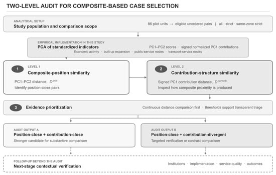
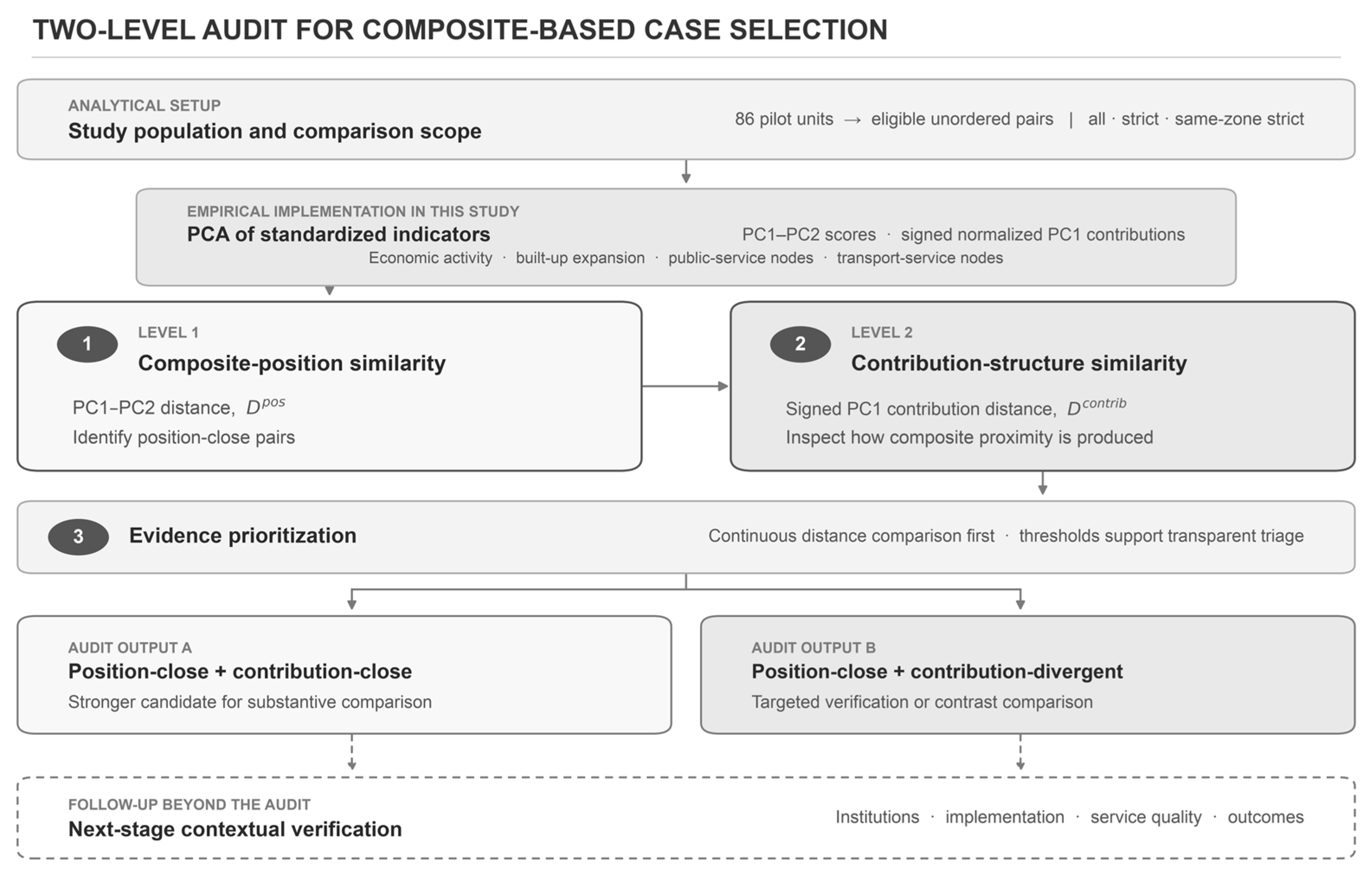
Composite similarity therefore supplies candidate pairs, and contribution inspection then grades the evidence each pair requires. Figure 1 summarizes the complete sequence and distinguishes the analytical setup, the PCA implementation used in this study, the two audit levels and outputs, and the contextual verification that follows.

Figure 1. Two-level contribution-structure audit as implemented in this study. The empirical implementation uses four dimensions—economic activity, built-up expansion, public-service nodes, and transport-service nodes—to construct PC1–PC2 positions and signed normalized PC1 contributions. Continuous distance comparison supports evidence prioritization. Both audit outputs lead to subsequent contextual verification. Solid elements represent the audit workflow and outputs, while dashed elements represent follow-up contextual verification beyond the audit.

This logic applies to any technique that admits an explicit, unit-specific decomposition into indicator contributions, so that the structure behind a position can be recovered and compared. The specific decomposition used here, and how composite-position and contribution-structure similarity are each measured, are specified in Section 3.

Within this scope, the framework tests the internal transparency of similarity-based classification: whether units placed close together exhibit similar indicator-contribution patterns. It serves as a pre-screening audit for case selection. Institutional comparability and policy transfer are evaluated through contextual evidence beyond the spatial indicators used here [4,5]. A pair that passes the two-level screen becomes a lower-risk candidate for contextual investigation.

3. Data and Methods

Section 3 operationalizes the two levels of comparability defined in Section 2. The unit pair is the unit of analysis, and eligible pairs are treated as interdependent comparisons among the 86 pilot units.

After Section 3.1 defines the analytical population and data foundation, Section 3.2, Section 3.3, Section 3.4 and Section 3.5 perform four linked functions. Section 3.2 converts source observations into comparable indicators and grouped dimensions. Section 3.3 constructs the composite representation and recovers unit-level contribution structures. Section 3.4 evaluates positional and structural comparability across eligible pairs and prioritizes cases for verification. Section 3.5 assesses the sensitivity of the main axis and candidate pool to alternative data and specifications.

3.1. Study Area, Analytical Sample, and Data

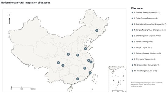
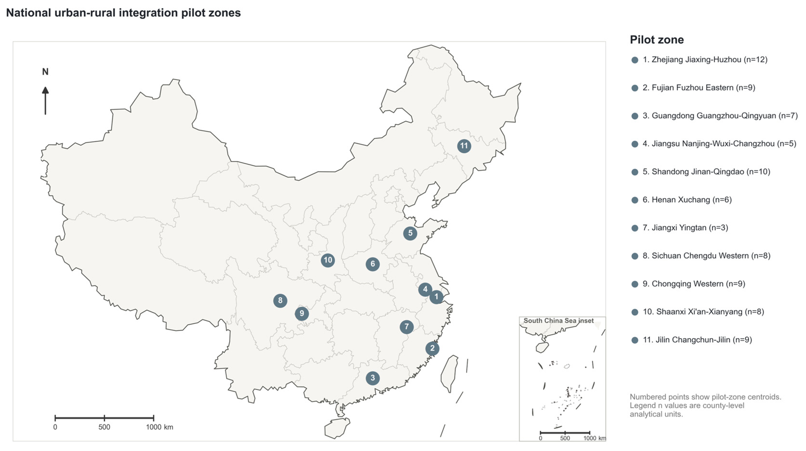
The analysis covers all 86 pilot units in China’s 11 national urban-rural integration pilot zones designated in 2019. A pilot zone is a policy-designated regional program; a pilot unit is one of its county-level analytical members, including counties, municipal districts, county-level cities, and several functional areas. Spatial unit is reserved for boundary matching. Figure 2 shows the national distribution of the 11 pilot zones and the number of pilot units in each zone. Supplementary Table S1 lists the members using the names in the national designation document [19].

Figure 2. Spatial distribution of the 11 national urban-rural integration pilot zones. Boundary, provincial, coastline, island, and South China Sea inset geometry are from the Ministry of Natural Resources Standard Map Service, map review number GS(2022)4309. Scale bars are provided for the main map and the South China Sea inset.

The study covers 2019–2023. The designation year, 2019, is the common baseline for all three data streams; 2023 is the common endpoint for a balanced record with fixed unit coverage and definitions. This common five-year window captures early post-designation change and meets the temporal requirements of the comparative screening design. The period includes the COVID-19 years and macroeconomic adjustment, so the indicators describe period-specific spatial-change profiles.

County boundaries are harmonized across nighttime-light, land-cover, and POI data. Functional-area or boundary-revised units requiring fallback built-up indicators remain in the full sample and are excluded from strict-sample checks.

Three data streams are used: VIIRS Annual VNL V2 nighttime lights for economic activity [30,31], the 30 m CLCD for built-up expansion [26], and 2019–2023 AMAP POIs for facility and transport nodes [24,27,28]. The main POI specification includes education, medical, public-leisure, and transport; the interrupted civic/social category serves as a quality diagnostic.

3.2. Indicator Construction and Grouped Dimensions

Seven indicators represent four dimensions: economic activity, built-up expansion, public-service facility nodes, and transport-service nodes. They measure 2020–2023 mean nighttime light relative to 2019, 2019–2023 built-up change, and category-year-adjusted POI density change.

For unit $i$, let ${\mathrm{N}\mathrm{T}\mathrm{L}}_{i,2019}$ be the mean nighttime-light intensity in 2019 and ${\mathrm{N}\sout{\mathrm{T}}\mathrm{L}}_{i,2020-2023}$ its 2020–2023 annual mean. Raw relative change is:

$$G_i^{\mathrm{N}\mathrm{T}\mathrm{L}}={\displaystyle \frac{{\mathrm{N}\sout{\mathrm{T}}\mathrm{L}}_{i,2020-2023}}{{\mathrm{N}\mathrm{T}\mathrm{L}}_{i,2019}}}-1.$$

The corresponding log change is:

$$L_i^{\mathrm{N}\mathrm{T}\mathrm{L}}=\mathrm{l}\mathrm{o}\mathrm{g}\left({\mathrm{N}\sout{\mathrm{T}}\mathrm{L}}_{i,2020-2023}\right)-\mathrm{l}\mathrm{o}\mathrm{g}\left({\mathrm{N}\mathrm{T}\mathrm{L}}_{i,2019}\right)=\mathrm{l}\mathrm{o}\mathrm{g}(1+G_i^{\mathrm{N}\mathrm{T}\mathrm{L}}).$$

All aggregated means are positive, so the log transformation uses no offset. The main specification removes the corresponding non-pilot provincial trend:

$$\mathsf{\Delta }{\mathrm{N}\mathrm{T}\mathrm{L}}_i^{\mathrm{a}\mathrm{d}\mathrm{j}}=L_i^{\mathrm{N}\mathrm{T}\mathrm{L}}-{\sout{L}}_{p\left(i\right),-\mathrm{p}\mathrm{i}\mathrm{l}\mathrm{o}\mathrm{t}}^{\mathrm{N}\mathrm{T}\mathrm{L}},$$

where ${\sout{L}}_{p\left(i\right),-\mathrm{p}\mathrm{i}\mathrm{l}\mathrm{o}\mathrm{t}}^{\mathrm{N}\mathrm{T}\mathrm{L}}$ is the province-level log trend excluding pilot units where available.

Let $B_{i,t}$ denote built-up share. Absolute expansion is measured by province-adjusted share change:

$$\mathsf{\Delta }{B}_i^{\mathrm{a}\mathrm{d}\mathrm{j}}=(B_{i,2023}-B_{i,2019})-{\sout{\mathsf{\Delta }B}}_{p\left(i\right),-\mathrm{p}\mathrm{i}\mathrm{l}\mathrm{o}\mathrm{t}},$$

where ${\sout{\mathsf{\Delta }B}}_{p\left(i\right),-\mathrm{p}\mathrm{i}\mathrm{l}\mathrm{o}\mathrm{t}}$ is the non-pilot provincial trend where available. Proportional expansion is:

$$R_i=\mathrm{l}\mathrm{o}\mathrm{g}\left({\displaystyle \frac{B_{i,2023}+ϵ}{B_{i,2019}+ϵ}}\right),$$

where $ϵ=0.002$ (0.2 percentage points) is added symmetrically to limit instability from near-zero baselines. This proportional measure complements absolute share change. Because the ratio lacks a matched non-pilot provincial trend, an all-unadjusted specification tests adjustment sensitivity. Boundary-related fallback values are flagged and excluded from strict-sample checks.

POI node changes are constructed after category-year audits. Civic/social is excluded because of a complete 2022 interruption; transport and public-leisure are retained with exclusion checks, and public-facility and sports/leisure subcategories are scaled separately before combination (Supplementary Table S4). Historical POIs are treated as map-observed node-density proxies. Cross-sectional benchmarks support education ($r=0.809$ with student density) and medical POIs ($r=0.919$ with bed density; Section 4.4); temporal validation requires longitudinal records. Sample-wide category-year shifts are scaled by:

$${\mathrm{S}\mathrm{c}\mathrm{a}\mathrm{l}\mathrm{e}}_{c,t}={\displaystyle \frac{{\mathrm{T}\mathrm{o}\mathrm{t}\mathrm{a}\mathrm{l}\mathrm{P}\mathrm{O}\mathrm{I}}_{c,2019}}{{\mathrm{T}\mathrm{o}\mathrm{t}\mathrm{a}\mathrm{l}\mathrm{P}\mathrm{O}\mathrm{I}}_{c,t}}},$$

where ${\mathrm{T}\mathrm{o}\mathrm{t}\mathrm{a}\mathrm{l}\mathrm{P}\mathrm{O}\mathrm{I}}_{c,t}$ is the sample total for category $c$ in year $t$; a zero total indicates data interruption. Adjusted counts are:

$${\mathrm{P}\mathrm{O}\mathrm{I}}_{i,c,t}^{\mathrm{a}\mathrm{d}\mathrm{j}}={\mathrm{P}\mathrm{O}\mathrm{I}}_{i,c,t}\times {\mathrm{S}\mathrm{c}\mathrm{a}\mathrm{l}\mathrm{e}}_{c,t}.$$

This scaling retains within-year cross-unit differences. Adjusted density change is:

$$\mathsf{\Delta }{\mathrm{P}\mathrm{O}\mathrm{I}}_{i,c}=\mathrm{l}\mathrm{o}\mathrm{g}\left(1+{\displaystyle \frac{{\mathrm{P}\mathrm{O}\mathrm{I}}_{i,c,2023}^{\mathrm{a}\mathrm{d}\mathrm{j}}}{{\mathrm{A}\mathrm{r}\mathrm{e}\mathrm{a}}_i}}\times 100\right)-\mathrm{l}\mathrm{o}\mathrm{g}\left(1+{\displaystyle \frac{{\mathrm{P}\mathrm{O}\mathrm{I}}_{i,c,2019}^{\mathrm{a}\mathrm{d}\mathrm{j}}}{{\mathrm{A}\mathrm{r}\mathrm{e}\mathrm{a}}_i}}\times 100\right).$$

The factor 100 provides numerical scaling. Total land area is the main denominator, and built-up area is tested for robustness. Education, medical, and public-leisure form the public-service indicators; transport forms the transport-service indicator.

The seven indicators are province-adjusted nighttime light; province-adjusted built-up share change; relative built-up expansion; education, medical, and public-leisure POI change; and transport POI change. A grouped specification averages z-standardized indicators within four dimensions:

$${\mathrm{E}\mathrm{c}\mathrm{o}\mathrm{n}\mathrm{o}\mathrm{m}\mathrm{i}\mathrm{c}}_i=z(\mathsf{\Delta }{\mathrm{N}\mathrm{T}\mathrm{L}}_i^{\mathrm{a}\mathrm{d}\mathrm{j}}),$$

$${\mathrm{B}\mathrm{u}\mathrm{i}\mathrm{l}\mathrm{t}}_i={\displaystyle \frac{1}{2}}\left[z(\mathsf{\Delta }{B}_i^{\mathrm{a}\mathrm{d}\mathrm{j}})+z(R_i)\right],$$

$${\mathrm{P}\mathrm{u}\mathrm{b}\mathrm{l}\mathrm{i}\mathrm{c}\mathrm{S}\mathrm{e}\mathrm{r}\mathrm{v}\mathrm{i}\mathrm{c}\mathrm{e}}_i={\displaystyle \frac{1}{3}}\left[z\left(\mathsf{\Delta }{\mathrm{P}\mathrm{O}\mathrm{I}}_{\mathrm{e}\mathrm{d}\mathrm{u},i}\right)+z\left(\mathsf{\Delta }{\mathrm{P}\mathrm{O}\mathrm{I}}_{\mathrm{m}\mathrm{e}\mathrm{d},i}\right)+z\left(\mathsf{\Delta }{\mathrm{P}\mathrm{O}\mathrm{I}}_{\mathrm{p}\mathrm{u}\mathrm{b}\mathrm{l}\mathrm{i}\mathrm{c}/\mathrm{l}\mathrm{e}\mathrm{i}\mathrm{s}\mathrm{u}\mathrm{r}\mathrm{e},i}\right)\right],$$

$${\mathrm{T}\mathrm{r}\mathrm{a}\mathrm{n}\mathrm{s}\mathrm{p}\mathrm{o}\mathrm{r}\mathrm{t}}_i=z\left(\mathsf{\Delta }{\mathrm{P}\mathrm{O}\mathrm{I}}_{\mathrm{t}\mathrm{r}\mathrm{a}\mathrm{n}\mathrm{s}\mathrm{p}\mathrm{o}\mathrm{r}\mathrm{t},i}\right).$$

The grouped analysis assigns equal weight to each dimension. Table 1 summarizes the conceptual dimensions, indicators, data sources, change definitions, and standardization used in the main specification.

Table 1. Indicators used to construct the observable spatial-change profile.

Dimension	Indicator	Data Source	Period	Change Definition	Standardization
Economic-activity change	Province-adjusted nighttime-light log change	VIIRS Annual VNL V2	2019–2023	log(mean 2020–2023)—log(2019), net of non-pilot provincial trend	z-score across 86 units
Built-up expansion	Province-adjusted built-up-share change	CLCD 30 m land-cover product	2019–2023	2019–2023 endpoint share change, net of non-pilot provincial trend	z-score across 86 units
Built-up expansion	Relative built-up expansion intensity	CLCD 30 m land-cover product	2019–2023	log[(built-up share 2023 + 0.002)/(built-up share 2019 + 0.002)]	z-score across 86 units
Public-service facility nodes	Education POI density change	AMAP education POIs	2019–2023	Endpoint log-density change after category-year scaling	z-score across 86 units
Public-service facility nodes	Medical POI density change	AMAP medical POIs	2019–2023	Endpoint log-density change after category-year scaling	z-score across 86 units
Public-service facility nodes	Public-leisure POI density change	AMAP public-facility and sports/leisure POIs	2019–2023	Endpoint log-density change after separate subcategory-year scaling	z-score across 86 units
Transport-service nodes	Transport POI density change	AMAP transport POIs	2019–2023	Endpoint log-density change after category-year scaling	z-score across 86 units

Note: Civic/social POI is a quality diagnostic because of its 2022 interruption. Transport POI is retained as a map-observed proxy and tested by exclusion.

3.3. PCA Specification and PC1 Contribution Decomposition

To connect composite positions with their indicator-level formation, PCA provides a low-dimensional, data-derived representation whose linear scores can be decomposed exactly. All seven indicators are z-standardized across the 86 units, and PCA is estimated from their correlation matrix. PCA is estimated for the seven indicators and for four grouped dimensions, re-standardized before analysis; both specifications retain PC1 and PC2 [32]. PC1 is oriented with positive built-up and economic-activity loadings and represents relative position within this population. PC1–PC2 defines composite position, while contribution decomposition uses the variance-maximizing PC1. KMO and Bartlett’s test assess sampling adequacy; weights, aggregation, uncertainty, and sensitivity are reported transparently [1,2].

A unit’s PC1 score gives its position on the dominant axis; signed contributions show how that position is formed:

$$S_i={\displaystyle \sum _{k=1}^K}{z}_{i,k}{w}_k,$$

where $z_{i,k}$ is unit $i$’s standardized value, $w_k$ is the PC1 weight, and $K$ is the number of indicators. The signed raw contribution is:

$$c_{i,k}=z_{i,k}{w}_k.$$

The contribution vector records the indicator pathway underlying PC1 position.

Signed contributions are normalized by total absolute magnitude:

$${\tilde{c}}_{i,k}={\displaystyle \frac{c_{i,k}}{{\sum }_{k=1}^K|c_{i,k}|}}.$$

L1 normalization preserves contribution direction and makes structures comparable across units.

The main specification compares signed normalized vectors. A sensitivity check compares $\left|{\tilde{c}}_{i,k}\right|$, capturing contribution magnitudes after removing direction.

3.4. Pairwise Comparability Check

Pairwise comparison connects the composite representation to case selection: composite proximity may arise from compensating indicator contributions, so position and contribution distances are examined together to prioritize contextual verification. The screen has four steps. First, unordered pairs are formed in three scopes: all 86 units; strict pairs that exclude the functional-area and boundary-fallback units noted in Section 3.1; and same-zone strict pairs that further restrict comparison to one national pilot zone. The last is the policy-focused baseline and limits broad differences in pilot setting.

Second, each pair receives a composite-position distance and a distance between signed normalized PC1 contribution vectors; smaller values indicate greater similarity.

Composite-position distance is measured as Euclidean distance in the PC1–PC2 score plane:

$$D_{ij}^{\mathrm{p}\mathrm{o}\mathrm{s}}=\sqrt{{\left({\mathrm{P}\mathrm{C}1}_i-{\mathrm{P}\mathrm{C}1}_j{)}^2+({\mathrm{P}\mathrm{C}2}_i-{\mathrm{P}\mathrm{C}2}_j\right)}^2}.$$

Contribution-structure distance is measured as Euclidean distance between the L1-normalized signed PC1 contribution vectors:

$$D_{ij}^{\mathrm{c}\mathrm{o}\mathrm{n}\mathrm{t}\mathrm{r}\mathrm{i}\mathrm{b}}=\sqrt{{\sum }_{k=1}^K{({\tilde{c}}_{i,k}-{\tilde{c}}_{j,k})}^2}.$$

With unit L1 norm, $D^{\mathrm{c}\mathrm{o}\mathrm{n}\mathrm{t}\mathrm{r}\mathrm{i}\mathrm{b}}$ ranges from 0 to 2; observed-sample quantiles describe its empirical scale.

$D^{\mathrm{p}\mathrm{o}\mathrm{s}}$ represents proximity in the displayed PC1–PC2 map, while $D^{\mathrm{c}\mathrm{o}\mathrm{n}\mathrm{t}\mathrm{r}\mathrm{i}\mathrm{b}}$ compares how the dominant PC1 axis is formed. A PC1-only position-distance check identifies 12 same-zone strict candidates, seven overlapping the baseline 11, and quantifies sensitivity to the positional definition.

Both distances derive from the same standardized indicators and PCA weights, so their association combines algebraic dependence with the observed arrangement of unit profiles. Offsetting contributions and PC2 allow similar positions to coexist with different PC1 structures. The correlation is therefore an internal-alignment diagnostic. Unit-label random coupling tests the observed unit correspondence against random reassignment; separating algebraic and empirical shares requires a different design that preserves the shared unit-level PCA construction.

Third, scatterplots, distributions, and Pearson and Spearman correlations describe both distances continuously within each scope. The Q25/Q75 flag then selects pairs at or below the 25th percentile of $D^{\mathrm{p}\mathrm{o}\mathrm{s}}$ and at or above the 75th percentile of $D^{\mathrm{c}\mathrm{o}\mathrm{n}\mathrm{t}\mathrm{r}\mathrm{i}\mathrm{b}}$ for verification. Scope-specific quantiles define a prioritization queue; Q20/Q80 and Q30/Q70 show threshold sensitivity.

Fourth, a unit-label random-coupling null fixes PC1–PC2 positions, reassigns signed normalized contribution vectors, and recomputes distances over 10,000 draws with a fixed seed. Each draw records Pearson and Spearman correlations and candidate counts. Reassignment is global for all and strict pairs and within pilot zones for the same-zone strict scope. Correlation means and 95% intervals summarize the random-coupling baseline; the one-sided lower-tail probability is the share of candidate counts at or below the observed value.

Further checks compare Q20/Q80, Q25/Q75, and Q30/Q70; cosine and correlation distances; Euclidean distance between the seven standardized indicators; and unnormalized raw-contribution distance:

$$D_{ij}^{\mathrm{r}\mathrm{a}\mathrm{w}}=\sqrt{{\sum }_{k=1}^K{(c_{i,k}-c_{j,k})}^2}.$$

The raw-contribution distance assesses sensitivity to L1 normalization when total raw contribution magnitudes are small.

3.5. Robustness and Comparability Checks

Robustness checks assess PC1 direction, explained variance, candidate count, and overlap with the baseline list. Re-estimated specifications report PC1 cosine similarity and the corresponding results.

The baseline is specified ex ante from the same-zone strict scope and data-credibility rules. Candidate priority reflects both the credibility of the leading indicators and recurrence across the main sensitivity variants. These variants restrict the sample, residualize initial levels, use unadjusted inputs, exclude selected POI categories, or replace normalized with raw contribution distance. Pairs appearing in one specification or sensitive to POI remain verification prompts. Province exclusions, grouped PCA, threshold changes, and complete POI removal provide broader sensitivity checks.

PCA checks compare seven indicators with grouped dimensions, exclude functional-area and boundary-fallback units, apply 1% and 5% winsorization, and omit each province in turn. An all-unadjusted nighttime-light and built-up-share specification tests adjustment sensitivity. Initial-level checks use level-change correlations and PCA of changes residualized on 2019 levels.

POI checks use a built-up-area denominator, exclude transport or public-leisure, remove all POIs, and compare education and medical levels with cross-sectional external facility benchmarks; longitudinal records are required for temporal validation. Pairwise checks vary thresholds, contribution-distance definitions, PC1-only and PC1–PC2 position distances, and raw and L1-normalized contributions. Administrative composition is assessed for PC1, PC2, and candidate rates. All analyses were implemented in Python 3.9.6.

4. Main Results

4.1. Indicator Correlations and PCA Structure

The seven-indicator matrix supports exploratory PCA (KMO $=0.749$; significant Bartlett’s test, ${\chi }^2=381.31$, $\mathrm{d}\mathrm{f}=21$). PCA is used as a descriptive projection of the standardized indicators.

The correlation matrix shows a coherent node block. Correlations among the three public-service facility-node indicators range from 0.855 to 0.922, and their correlations with transport-service node change range from 0.520 to 0.627. Education, medical, public-leisure, and transport-service POI changes therefore share a common pattern.

Economic-activity and built-up changes are weakly associated: nighttime-light change correlates with built-up share change at $r=-0.072$ and with relative built-up expansion at $r=0.191$. The two built-up indicators correlate at $r=0.329$ and capture complementary absolute and proportional changes.

Relative built-up expansion has the strongest negative correlations with education ($r=-0.402$), medical ($r=-0.425$), and public-leisure ($r=-0.334$) POI changes. This pattern motivates the PCA.

Correlations between 2019 levels and subsequent changes are $-0.079$ for nighttime light, $+0.493$ for built-up share, $-0.032$ for relative built-up expansion, $-0.160$ for education, $-0.152$ for medical, $-0.436$ for public-leisure, and $-0.613$ for transport nodes. Relative built-up expansion shows little initial-level dependence, while public-leisure and transport show stronger convergence patterns. Section 4.4 and Supplementary Tables S6 and S7 report the residualized checks.

For the 81 units with complete built-up-area denominators, recomputing POI density per built-up area preserves the PC1 direction (cosine similarity $=0.999$; Section 4.4), supporting denominator robustness.

In the seven-indicator PCA, PC1 and PC2 explain 50.9% and 16.9% of standardized variance, respectively, for a cumulative 67.8%. PC1 is oriented so that economic-activity and built-up indicators load positively.

PC1 has positive weights for relative built-up expansion ($+0.278$), nighttime-light change ($+0.193$), and built-up share change ($+0.133$), and negative weights for education ($-0.485$), medical ($-0.497$), public-leisure ($-0.489$), and transport-service nodes ($-0.382$).

PC1 therefore contrasts built-up/economic-activity changes with observed facility/transport-node signals. Its positive side combines stronger built-up or activity signals with weaker standardized node-density growth, and its negative side shows the reverse. Historical POI records make this an observed spatial-data pattern: external cross-sectional benchmarks provide stronger support for education and medical nodes, while public-leisure and transport remain more sensitive to platform maintenance and category coverage. Direct assessment of facility expansion requires longitudinal administrative or field records.

The civic/social category is excluded from the main specification because of its 2022 category-year interruption. Removing transport as an additional check yields a six-indicator PC1 that explains 52.2% of variance and has cosine similarity of 0.999 with the baseline direction over shared indicators. The axis direction is stable, while platform maintenance, category coverage, low-base convergence, and real facility change remain sources of uncertainty in the node-side signal.

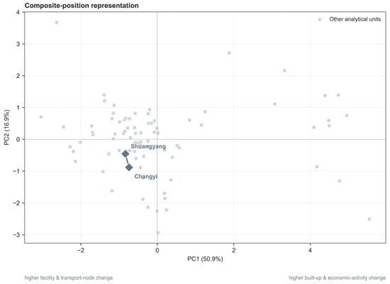
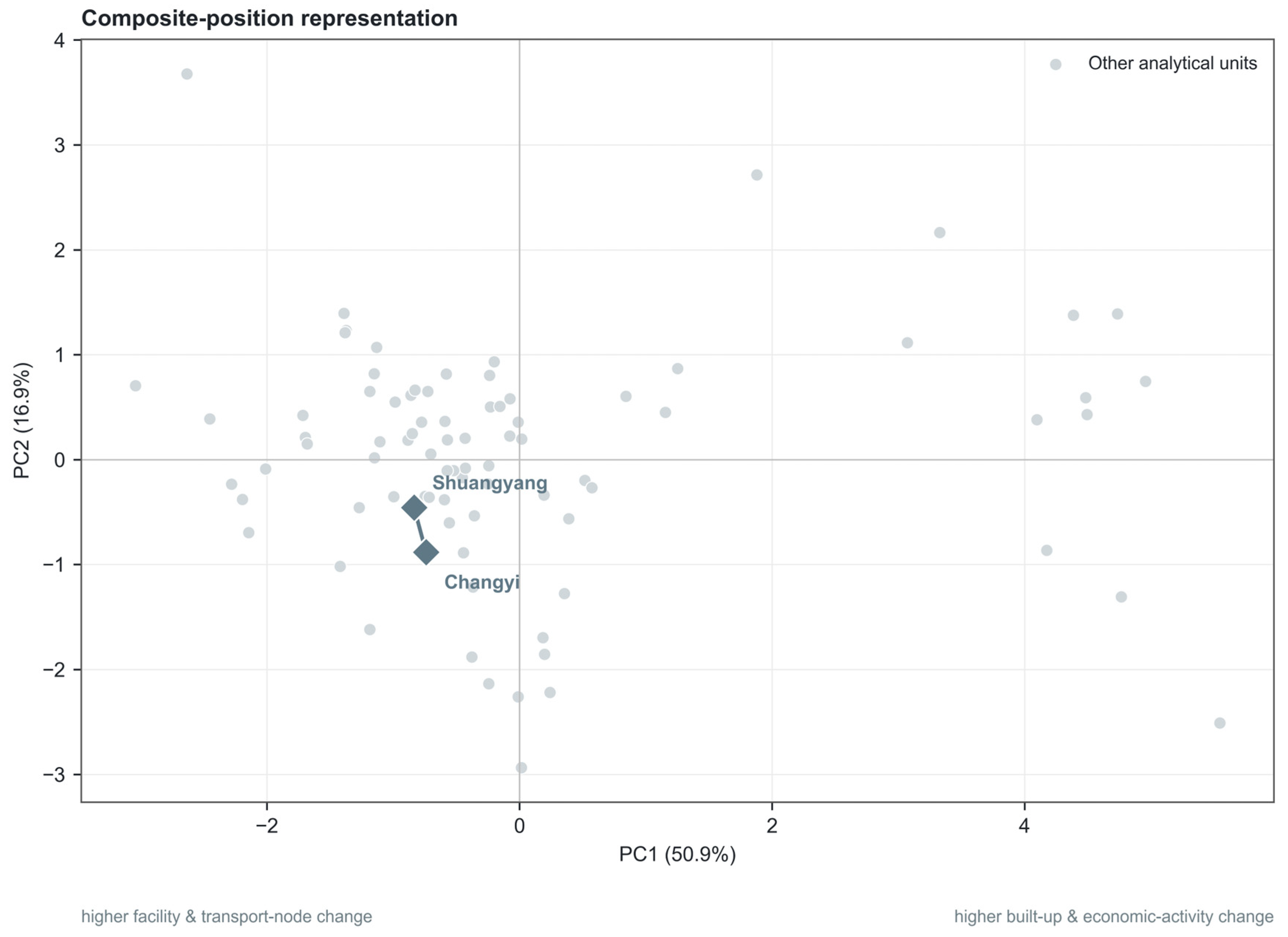
PC2 mainly separates combinations of economic-activity change and built-up expansion. Its largest weights are built-up share change ($-0.820$), relative built-up expansion ($-0.381$), and nighttime-light change ($+0.343$); the four node indicators have smaller weights. Table 2 reports the component loadings, PC1 scoring weights, and explained variance, while Figure 3 displays the corresponding PC1–PC2 positions and highlights the Shuangyang–Changyi pair.

Table 2. PCA loadings, PC1 scoring weights, and explained variance.

Dimension	Indicator/Statistic	PC1 Loading	PC2 Loading	PC1 Scoring Weight
Economic activity	Nighttime light	+0.365	+0.373	+0.193
Built-up expansion	Built-up share	+0.250	−0.892	+0.133
Built-up expansion	Relative built-up expansion	+0.524	−0.414	+0.278
Public-service nodes	Education nodes	−0.915	−0.212	−0.485
Public-service nodes	Medical nodes	−0.939	−0.124	−0.497
Public-service nodes	Public-leisure nodes	−0.924	−0.076	−0.489
Transport nodes	Transport nodes	−0.722	+0.106	−0.382
Variance summary	Explained variance share	50.9%	16.9%

Note: PC1 and PC2 explain 50.9% and 16.9% of the total standardized variance, respectively; their cumulative share is 67.8%. Composite-position similarity ($D^{\mathrm{p}\mathrm{o}\mathrm{s}}$) is computed in the PC1–PC2 plane; contribution-structure similarity ($D^{\mathrm{c}\mathrm{o}\mathrm{n}\mathrm{t}\mathrm{r}\mathrm{i}\mathrm{b}}$) is based on unit-specific signed normalized contributions to PC1 only.

Figure 3. PC1–PC2 composite positions of the 86 pilot units. Shuangyang and Changyi are highlighted, and the connecting segment shows their proximity in composite space.

The four-dimensional grouped PCA retains the same orientation (KMO $=0.633$; significant Bartlett’s test, ${\chi }^2=53.88$, $\mathrm{d}\mathrm{f}=6$). Its modest KMO supports its use as a structural check, with the seven-indicator PCA remaining the main representation.

Grouped PC1 and PC2 explain 48.4% and 23.3% of variance. PC1 weights are $+0.335$ for economic activity, $+0.406$ for built-up expansion, $-0.611$ for public-service facility nodes, and $-0.591$ for transport-service nodes; PC2 separates economic activity (−$0.817$) from built-up expansion (+$0.573$). The persistent main-axis direction supports its structural interpretation.

Overall, the dominant axis describes a 2019–2023 contrast between built-up/economic-activity and facility/transport-node signals across the 86 units, answering the first research question. Section 4.2 examines whether nearby PC1–PC2 positions share similar signed PC1 contributions.

4.2. PC1 Contribution Structure

To examine how PCA positions are produced, PC1 scores are decomposed into signed indicator contributions. A unit’s PC1 score is the sum of standardized indicator values multiplied by the corresponding PC1 scoring weights. The contribution vector shows whether each indicator pushes the unit toward the positive or negative side of PC1 and how large that contribution is relative to the other indicators.

The decomposed results show diverse leading indicators across PC1 positions. Using the largest absolute normalized contribution within each unit, the leading contributor is education POI for 20 units, public-leisure POI for 19, transport POI for 19, medical POI for 12, nighttime light for 8, relative built-up expansion for 6, and built-up share change for 2. The mean absolute normalized contribution shares are also larger for the node indicators (0.174 for education, 0.174 for medical, 0.190 for public-leisure, and 0.168 for transport) than for nighttime light (0.117), relative built-up expansion (0.117), and built-up share change (0.061). This pattern indicates that many units’ PC1 positions are generated by facility/transport-node contributions as much as by construction or activity signals.

The signed contributions clarify the interpretation of the two sides of PC1. Among the 25 units on the positive side of PC1, the median combined signed contribution from the facility/transport-node indicators is $+0.702$, whereas the median combined contribution from the economic-activity and built-up indicators is $+0.121$. Because the node indicators have negative PC1 weights, positive node-block contributions generally mean below-average facility/transport-node growth pushing a unit toward the positive side. Among the 61 units on the negative side of PC1, the corresponding medians are $-0.636$ for the facility/transport-node block and $-0.089$ for the economic-activity and built-up block. The PC1 contrast is a relative axis in which weak or strong node growth contributes substantially to position.

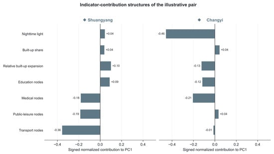
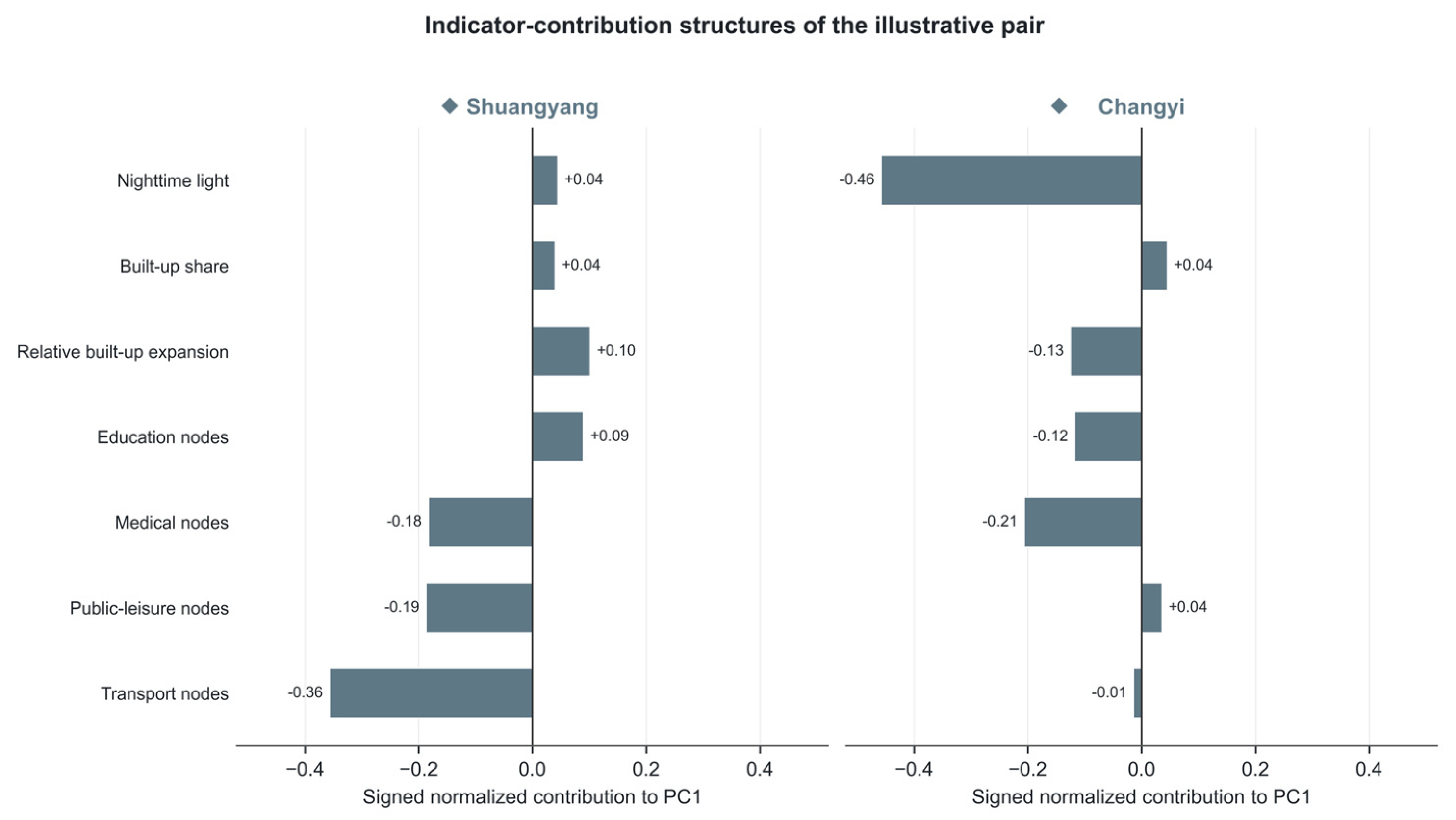
The Shuangyang District–Changyi District pair illustrates why this matters for pairwise comparison. Their PC1 scores are close ($-0.835$ and $-0.740$, respectively; absolute difference $=0.096$), but their contribution structures differ. Shuangyang’s largest signed normalized contribution is transport POI ($-0.356$), followed by public-leisure POI ($-0.187$) and medical POI ($-0.182$); Changyi’s largest contribution is nighttime light ($-0.457$), followed by medical POI ($-0.206$) and relative built-up expansion ($-0.125$). The leading pairwise contribution differences are therefore nighttime light (absolute difference $=0.502$) and transport POI (absolute difference $=0.342$). Although the pair is close in composite space ($D^{\mathrm{p}\mathrm{o}\mathrm{s}}=0.438$), its contribution distance ($D^{\mathrm{c}\mathrm{o}\mathrm{n}\mathrm{t}\mathrm{r}\mathrm{i}\mathrm{b}}=0.716$) lies at approximately the 90th percentile of the same-zone strict distribution. Similar PC1 placement can thus reflect distinct indicator pathways.

Available contextual evidence makes these differences substantively plausible follow-up questions. Shuangyang is an outer district of Changchun with extensive rural functions; its 2021–2025 plan emphasizes metropolitan connection, integrated urban–rural transport, modern agriculture, and the development of a new urban district [33]. Changyi, by contrast, contains Jilin City’s principal railway, urban-bus, and long-distance-coach hub as well as established commercial and industrial areas [34]. Read against that context, Shuangyang’s relatively strong map-recorded transport-node growth and Changyi’s relatively weak nighttime-light change point to different observable pathways behind their nearby PCA positions. Causal assessment of these pathways requires annual transport-facility inventories, construction histories, business activity records, and local planning evidence before the pair is used for mechanism comparison. Figure 4 visualizes the pair’s signed PC1 contribution profiles and the indicators responsible for their structural divergence.

Figure 4. Signed normalized PC1 contributions for the Shuangyang–Changyi pair. Positive contributions extend right and negative contributions extend left.

The comparison therefore pairs PC1–PC2 proximity with signed normalized PC1 contributions. It makes visible the different mixtures of node, activity, and built-up signals that can occupy the same coordinate region.

4.3. Pairwise Comparability Check and Evidence Grading

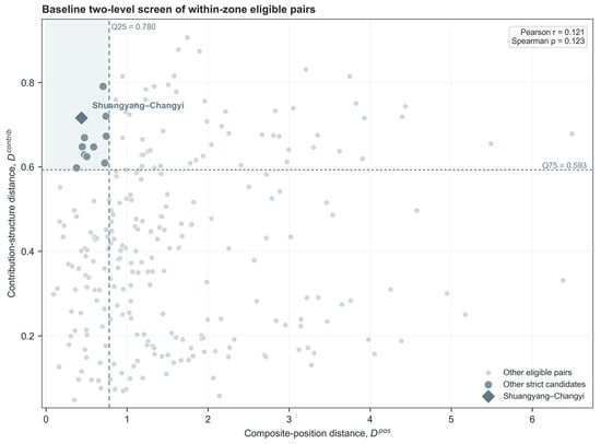
The pairwise comparability check first examines continuous distances across all 3655 possible pairs. Pearson and Spearman correlations are 0.543 and 0.543 across all pairs and 0.578 and 0.588 across 2850 strict pairs. Within the 258 same-zone strict pairs, the association is much weaker (Pearson $r=0.121$; Spearman $\rho =0.123$). Figure 5 displays every same-zone strict pair, including the flagged cases.

Figure 5. Baseline two-level screen of the 258 same-zone strict pairs. Dashed lines mark the Q25 threshold for composite-position distance and the Q75 threshold for contribution-structure distance; Shuangyang–Changyi is highlighted.

These correlations describe internal alignment between two PCA-derived measures. Under unit-label random coupling, the mean Pearson correlation is 0.000 across all pairs (95% interval: $-0.066$ to $0.082$), 0.000 across strict pairs ($-0.065$ to $0.085$), and $-0.153$ across same-zone strict pairs ($-0.240$ to $-0.044$). The observed positive correlations exceed the relationships generated from the two marginal distance distributions under random reassignment. Because the benchmark reassigns the unit-level correspondence between PCA positions and PCA-derived contribution vectors, it estimates the strength of internal alignment under random coupling. Separating algebraic and empirical shares requires a different identification design.

The Q25/Q75 flag is then used for verification triage. It identifies 57 pairs in the full scope, 39 in the strict scope, and 11 among the 258 same-zone strict pairs. In the same-zone strict scope, the numerical cutoffs are $D^{\mathrm{p}\mathrm{o}\mathrm{s}}\le 0.780$ and $D^{\mathrm{c}\mathrm{o}\mathrm{n}\mathrm{t}\mathrm{r}\mathrm{i}\mathrm{b}}\ge 0.593$; observed $D^{\mathrm{c}\mathrm{o}\mathrm{n}\mathrm{t}\mathrm{r}\mathrm{i}\mathrm{b}}$ values range from 0.049 to 0.906, with a median of 0.406. The count changes from 5 under Q20/Q80 to 11 under Q25/Q75 and 12 under Q30/Q70. Accordingly, the 11 pairs form a setting-specific baseline verification queue prioritized for follow-up.

The random-coupling candidate-count benchmark yields means of 228.1 candidates across all pairs (95% interval: 183–270), 178.3 among strict pairs (139–213), and 17.2 among same-zone strict pairs (11–23), compared with 57, 39, and 11 observed. The lower-tail permutation probabilities are below 0.001 for the first two scopes and 0.036 for the same-zone strict scope. These results show that close-position/high-contribution-distance cases are less frequent than under reassignment, while preserving a limited exception tail for inspection. Full null results are reported in Supplementary Table S5.

Because PC1 combines positive built-up/economic-activity loadings with negative facility/transport-node loadings, the exception tail can contain nearby composite positions produced through offsetting contributions. The baseline 11-pair triage pool is summarized in Table 3, with full two-indicator divergence profiles in Supplementary Table S2.

Table 3. Baseline same-zone strict triage pool.

Pair	Pilot Zone	${\mathit{D}}^{\mathbf{p}\mathbf{o}\mathbf{s}}$	${\mathit{D}}^{\mathbf{c}\mathbf{o}\mathbf{n}\mathbf{t}\mathbf{r}\mathbf{i}\mathbf{b}}$	Leading Divergence	Evidence Grade
Shuangyang District–Fengman District	Jilin Changchun-Jilin	0.704	0.791	relative built-up expansion (0.458)	Hard-signal-led
Fengman District–Yongji County	Jilin Changchun-Jilin	0.741	0.720	NTL (0.471)	Hard-signal-led
Shuangyang District–Changyi District	Jilin Changchun-Jilin	0.438	0.716	NTL (0.502)	Hard-signal-led
Rongchang District–Jiangjin District	Chongqing Western	0.743	0.673	transport POI (0.487)	Cautious-POI-led
Pengzhou City–Pujiang County	Sichuan Chengdu Western	0.474	0.669	transport POI (0.591)	Cautious-POI-led
Zhangqiu District–Laixi City	Shandong Jinan-Qingdao	0.448	0.648	transport POI (0.433)	Cautious-POI-led
Zichuan District–Laixi City	Shandong Jinan-Qingdao	0.589	0.647	public-leisure POI (0.466)	Cautious-POI-led
Dujiangyan City–Pujiang County	Sichuan Chengdu Western	0.474	0.629	transport POI (0.528)	Cautious-POI-led
Rongchang District–Hechuan District	Chongqing Western	0.503	0.624	transport POI (0.463)	Cautious-POI-led
Shizhong District–Laixi City	Shandong Jinan-Qingdao	0.724	0.609	medical POI (0.452)	Verified-POI-led
Zhangqiu District–Jimo District	Shandong Jinan-Qingdao	0.377	0.598	transport POI (0.399)	Cautious-POI-led

Note: This specification-dependent triage pool is accompanied by full two-indicator divergence profiles in Supplementary Table S2.

Table 3 is a specification-bound triage list. Three hard-signal-led pairs—Shuangyang–Changyi, Shuangyang–Fengman, and Fengman–Yongji—receive the strongest follow-up priority because nighttime light or built-up expansion leads their divergence. Shizhong–Laixi is led by benchmark-supported medical POI. The remaining seven transport- or public-leisure-led pairs require verification against local inventories, networks, and plans before substantive interpretation. Supplementary Table S2 reports the two leading differences for each pair, and Section 4.4 shows how membership changes across specifications.

Section 4 therefore establishes the baseline empirical pattern: composite-position similarity and contribution-structure similarity usually align, while a bounded set of close-position pairs requires contribution-level inspection.

4.4. Robustness and Diagnostic Checks

Robustness is evaluated for three properties: the direction of PC1, the variance it explains, and the composition of the candidate pool. Table 4 summarizes the main checks; Supplementary Tables S3–S8 provide the detailed counts, overlaps, POI diagnostics, random-coupling baseline, initial-level checks, and administrative-composition values.

Table 4. Consolidated robustness results across specifications.

Specification	PC1 Var. (%)	Cosine vs. Baseline	Same-Zone Strict Candidates	Overlap with Baseline 11
Baseline (7-indicator)	50.9	—	11	—
Grouped-dimension	48.4	orientation preserved	—	—
Strict sample	52.6	0.999	—	—
Winsorization (1%/5%)	—	>0.999	—	—
Leave-Zhejiang-out	34.1	0.917	2	1
Initial-level residualized	51.8	0.994	15	5
Unadjusted NTL + built-up	56.4	0.972	9	2
Remove public-leisure	46.0	0.999	11	7
Remove transport	—	0.999	9	4
POI density per built-up area	52.8	0.999	—	—
Remove all POI (3-indicator)	45.1	—	2	0
PC1-only position distance	—	—	12	7
Raw contribution distance	—	—	6	3

Note: Cosine similarity is computed against the baseline PC1 loading vector over shared indicators where applicable. Candidate counts and overlaps are reported in the same-zone strict scope where reconstructed. Specifications with reported cosine values preserve the PC1 direction (0.917–0.999), whereas the explained-variance share and candidate membership vary with specification. The raw contribution-distance row changes the contribution-distance metric while holding the PCA estimates fixed. Detailed robustness counts and overlaps are in Supplementary Tables S3 and S6.

The grouped-dimension, strict-sample, and winsorized specifications all retain the full-sample PC1 orientation, supporting the direction of the built-up/economic-activity versus facility/transport-node contrast. Regional composition affects PC1 strength more substantially. Zhejiang contains 12 of the 86 units and accounts for 72.0% of the full-sample PC1 score sum of squares; when Zhejiang is removed and PCA is refitted, PC1 explains 34.1%, compared with 50.9% in the full sample. The contrast remains recognizable (cosine similarity = 0.917): built-up share change stays positive ($+0.275$), while education, medical, public-leisure, and transport nodes stay negative ($-0.468$, $-0.537$, $-0.535$, and $-0.361$). Nighttime-light change and relative built-up expansion shrink to near-zero weights, and the same-zone strict scan identifies two candidates among 192 eligible pairs, one overlapping the baseline 11.

Initial levels and adjustment choices affect the candidate pool more than the axis direction. The initial-level correlations reported in Section 4.1 show little baseline dependence for nighttime light, relative built-up expansion, education nodes, or medical nodes, moderate dependence for built-up share, and stronger convergence patterns for public-leisure and transport nodes. Residualizing every change indicator against its 2019 level leaves the axis direction essentially unchanged (cosine similarity = 0.994), while replacing the province-adjusted nighttime-light and built-up-share indicators with unadjusted changes also preserves the direction (cosine similarity = 0.972). The residualized and unadjusted specifications identify 15 and 9 candidates, with 5 and 2 overlaps with the baseline 11, respectively.

POI uncertainty affects the full empirical representation as well as the interpretation of individual flagged pairs. Four of the seven indicators are POI-derived. Because they carry the largest absolute PC1 weights, POI measures also lead most baseline candidates. The category-year audit isolates the civic/social interruption, while cross-sectional benchmarks support observed education and medical POI density (student-density $r=0.809$; medical-bed-density $r=0.919$). Longitudinal external records are required to validate change over time. Removing public-leisure preserves the axis direction (cosine similarity = 0.999) and retains seven baseline candidates. Removing transport also preserves the shared PC1 direction (cosine similarity = 0.999), while the same-zone strict pool falls to nine candidates with four overlaps. Removing all POI indicators produces a three-indicator representation in which PC1 explains 45.1% of variance and two same-zone strict discrepancies remain, each outside the baseline 11. Thus, the general audit logic applies across data types, while the substantive axis, candidate count, and candidate identities in this application depend on the POI variables. Spatially uneven platform backfilling could itself generate part of the facility/transport-node contrast, so POI-led differences serve as verification prompts. Recomputing POI density per built-up area preserves direction (cosine similarity = 0.999), while the temporal-validity assessment continues to require longitudinal benchmark data.

Candidate sets also appear under several screening variants, and their size depends on the metric. Across the Q20/Q80, Q25/Q75, and Q30/Q70 thresholds, the same-zone strict scan identifies 5, 11, and 12 pairs; alternative cosine, correlation, original-indicator, and PC1-only definitions also return exception sets. The L1-normalized signed contribution distance is sensitive to low total raw contribution magnitude: the baseline 11 pairs have a lower median average raw contribution magnitude than the full same-zone strict scope (1.069 versus 1.331). Using unnormalized raw contribution distance reduces the same-zone strict pool to six candidates, three of which overlap the baseline 11, including Shuangyang–Changyi. Thus, L1 normalization enlarges part of the tail, while the remaining discrepancies also appear under the raw contribution distance. Administrative type accounts descriptively for 1.0% of PC1 variation and 17.0% of PC2 variation, and candidate rates are similar for same-type pairs (7/155, 4.5%) and different-type pairs (4/103, 3.9%). Taken together, the checks support a recognizable association direction and a limited exception tail, while showing that PC1 strength and candidate identity are specification-dependent.

5. Discussion

5.1. From Composite-Indicator Robustness to Pairwise Comparability

Composite-indicator scholarship has shown that scores and rankings can change with decisions about normalization, weighting, and aggregation as well as with the treatment of uncertainty; these decisions should therefore be transparent [1,2,3]. The present results confirm the importance of that agenda and extend it downstream. An axis direction or aggregate ranking can remain reasonably robust while two nearby units occupy their positions through different signed indicator combinations. The proposed distinction between composite-position similarity and contribution-structure similarity evaluates the internal support for a particular comparison alongside the stability of the index as a whole.

The results also give a bounded empirical illustration of equifinality [29]. The positive association between the two PCA-derived distance measures indicates internal alignment within the observed data because both distances reuse the same standardized indicators and PCA weights. The random-coupling comparison shows stronger alignment in the observed unit-level correspondence than under reassignment of the contribution profiles. The close-position/divergent-structure tail identifies compensating indicator pathways within apparently similar aggregate positions. Together, these results show how contribution inspection changes the evidential status of plausible pairwise comparisons.

Substantively, the main axis is consistent with the land-system view that built-up land, activity intensity, service provision, and infrastructure make distinct contributions to territorial change [15,16,17,18]. The weak relationship between nighttime-light change and built-up expansion, together with the opposing facility/transport-node block, indicates heterogeneous observable trajectories under a shared mandate. The axis provides a sample- and measurement-dependent description of the 2019–2023 population. Assessment of causal relationships between construction and services requires a causal research design.

5.2. Contributions, Limitations, and Future Research

The contributions are theoretical, methodological, and empirical. Theoretically, the study distinguishes positional comparability from contribution-structure comparability and identifies contribution structure as an additional case-selection criterion when aggregate positions allow compensating pathways. Methodologically, it provides a reproducible audit that combines contribution decomposition with continuous distance and sensitivity analysis to grade the evidence for candidate pairs. Empirically, it maps all 86 pilot units and shows how land and activity changes combine with changes in facility and transport nodes under a shared mandate.

The methodological contribution also extends to composite-based comparison of countries, regions, cities, and public-service systems [1,3]. It applies when indicator definitions are comparable, unit-level contributions can be recovered, and specification sensitivity is reported. In China’s pilot-program context, the framework can be implemented in three stages. National and regional authorities responsible for the pilot program first use composite-position distance to identify pilot-unit comparisons relevant to a shared reform task. Local authorities then assemble a common evidence dossier—planning and implementation records, fiscal and facility inventories, transport networks, population and service outcomes, and field verification—for pairs prioritized by contribution inspection. Pairs aligned at both levels can advance to substantive comparative evaluation, while structure-divergent pairs serve as contrast cases or remain in verification; decisions on experience replication follow from the contextual evidence [4,5,19,23].

The study has three methodological limitations: the two distances share the same PCA construction, position uses PC1–PC2 while contribution uses PC1, and the Q25/Q75 screening rule is setting-specific. The random-coupling benchmark evaluates internal alignment against reassigned marginal distance structures; separating the algebraic share of the correlation requires an independent design. The PC1-only and alternative-threshold tests quantify the corresponding design sensitivity, while the continuous distances carry the main comparative information.

Additional limitations concern the data and scope of inference. Four of seven indicators are POI-derived and carry large PC1 weights. Category-year scaling and cross-sectional benchmarks for education and medical POIs support comparability, while temporal validation requires longitudinal records. Uncertainty remains because platform coverage can expand unevenly and because classification, registration, or local backfilling practices can change; the POI-free analysis accordingly produces candidates outside the baseline set [27]. The 2019–2023 window also spans pandemic disruption and recovery. These conditions may affect nighttime lights and POI endpoints through changes in real activity—including restrictions, reopening, operating hours, and temporary closures—as well as through delayed registration or database updates [35,36]. Province adjustment absorbs common province-level trends, while local exposure and platform effects remain. The audit framework can be applied across periods. The estimated PCA axis, screening thresholds, and candidate identities are specific to a window spanning pandemic disruption and recovery. Applications to normal or post-pandemic periods require re-estimation with updated observations. Because the linear PCA representation depends on standardization and on the selected population and indicators, the descriptive contribution-structure analysis supports pre-screening. Mechanisms and transferability must then be established from contextual evidence about local development history, institutional and fiscal capacity, population mobility and service quality, implementation, and outcomes. The audit’s application scope is case selection for comparison or policy learning when composite proximity guides which units are compared. Other uses of composite indicators fall outside this scope.

Future research should extend the present audit in three directions. First, longitudinal changes in POIs should be validated against independent administrative records to distinguish substantive service change from platform updates. Second, the framework should be re-estimated using normal or post-pandemic observation windows to assess the temporal stability of the PCA axis and the candidate pairs. Third, contribution-structure screening should be combined with contextual case evidence and, where feasible, causal research designs to examine mechanisms and determine whether apparently comparable pilot experiences are transferable.

6. Conclusions

This study examined multidimensional land-system change in 86 urban-rural integration pilot units during 2019–2023 through standardized indicators and PCA-based comparisons of composite positions and contribution structures. The results reveal a recurring contrast between built-up/economic-activity signals and facility/transport-node signals. This pattern remains visible across the grouped-dimension, strict-sample, winsorized, and indicator-exclusion checks, although its strength varies with regional composition and POI measurement.

Composite-position and contribution-structure distances are positively associated across all 3655 pairs, with a weaker association among the 258 same-zone strict pairs. The baseline Q25/Q75 screen identifies 11 pairs in which close composite positions coexist with divergent contribution structures; sensitivity tests yield 5–12 pairs and alter candidate membership. Taken together, composite position and indicator composition provide a clearer basis for selecting cases for contextual verification and comparative learning among the pilot units.

References

- OECD; Joint Research Centre of the European Commission (JRC). Handbook on Constructing Composite Indicators: Methodology and User Guide; OECD Publishing: Paris, France, 2008. [Google Scholar] [CrossRef] [Scilit]
- Saisana, M.; Saltelli, A.; Tarantola, S. Uncertainty and sensitivity analysis techniques as tools for the quality assessment of composite indicators. J. R. Stat. Soc. Ser. A (Stat. Soc.) 2005, 168, 307–323. [Google Scholar] [CrossRef] [Scilit]
- Greco, S.; Ishizaka, A.; Tasiou, M.; Torrisi, G. On the methodological framework of composite indices: A review of the issues of weighting, aggregation, and robustness. Soc. Indic. Res. 2019, 141, 61–94. [Google Scholar] [CrossRef] [Scilit]
- Dolowitz, D.P.; Marsh, D. Learning from abroad: The role of policy transfer in contemporary policy-making. Governance 2000, 13, 5–23. [Google Scholar] [CrossRef] [Scilit]
- Peck, J.; Theodore, N. Mobilizing policy: Models, methods, and mutations. Geoforum 2010, 41, 169–174. [Google Scholar] [CrossRef] [Scilit]
- Seawright, J.; Gerring, J. Case selection techniques in case study research: A menu of qualitative and quantitative options. Political Res. Q. 2008, 61, 294–308. [Google Scholar] [CrossRef] [Scilit]
- Chen, K.; Long, H.; Liao, L.; Tu, S.; Li, T. Land use transitions and urban-rural integrated development: Theoretical framework and China’s evidence. Land Use Policy 2020, 92, 104465. [Google Scholar] [CrossRef] [Scilit]
- Niu, B.; Ge, D.; Sun, J.; Sun, D.; Ma, Y.; Ni, Y.; Lu, Y. Multi-scales urban-rural integrated development and land-use transition: The story of China. Habitat Int. 2023, 132, 102744. [Google Scholar] [CrossRef] [Scilit]
- Shen, C.; Shi, L.; Wu, X.; Ding, J.; Wen, Q. Exploring the coupling coordination and key factors between urban-rural integrated development and land-use efficiency in the Yellow River Basin. Land 2023, 12, 1583. [Google Scholar] [CrossRef] [Scilit]
- Zeng, Q.; Chen, X. Identification of urban-rural integration types in China: An unsupervised machine learning approach. China Agric. Econ. Rev. 2023, 15, 400–415. [Google Scholar] [CrossRef] [Scilit]
- Zhang, N.; Yao, Y.; Wang, L.; Li, Q. Spatial-temporal coupling analysis of land use function and urban-rural integration in Heilongjiang, China. Land 2023, 12, 2152. [Google Scholar] [CrossRef] [Scilit]
- Tacoli, C. Rural-urban interactions: A guide to the literature. Environ. Urban. 1998, 10, 147–166. [Google Scholar] [CrossRef]
- OECD. Rural-Urban Partnerships: An Integrated Approach to Economic Development; OECD Rural Policy Reviews; OECD Publishing: Paris, France, 2013. [Google Scholar] [CrossRef] [Scilit]
- Zhang, S.; Sun, K.; Zhao, H.; Yao, H.; Shen, L. Research on the construction and practice of an urban-rural integration planning model from the perspective of element flow: A case study of Xiuzhou District, Jiaxing City. Land 2025, 14, 1067. [Google Scholar] [CrossRef] [Scilit]
- Turner, B.L.; Lambin, E.F.; Reenberg, A. The emergence of land change science for global environmental change and sustainability. Proc. Natl. Acad. Sci. USA 2007, 104, 20666–20671. [Google Scholar] [CrossRef] [Scilit] [PubMed]
- Verburg, P.H.; Erb, K.-H.; Mertz, O.; Espindola, G. Land system science: Between global challenges and local realities. Curr. Opin. Environ. Sustain. 2013, 5, 433–437. [Google Scholar] [CrossRef] [Scilit] [PubMed]
- Verburg, P.H.; Crossman, N.; Ellis, E.C.; Heinimann, A.; Hostert, P.; Mertz, O.; Nagendra, H.; Sikor, T.; Erb, K.-H.; Golubiewski, N.; et al. Land system science and sustainable development of the earth system: A global land project perspective. Anthropocene 2015, 12, 29–41. [Google Scholar] [CrossRef] [Scilit]
- Liu, J.; Hull, V.; Batistella, M.; DeFries, R.; Dietz, T.; Fu, F.; Hertel, T.W.; Izaurralde, R.C.; Lambin, E.F.; Li, S.; et al. Framing sustainability in a telecoupled world. Ecol. Soc. 2013, 18, 26. [Google Scholar] [CrossRef] [Scilit]
- National Development and Reform Commission of the People’s Republic of China (NDRC). Notice on Carrying Out the Work of National Urban-Rural Integration Development Pilot Zones (Fa Gai Gui Hua [2019] No. 1947). 2019. Available online: https://www.ndrc.gov.cn/xwdt/ztzl/xxczhjs/ghzc/202012/t20201225_1260277.html (accessed on 30 May 2026).
- Heilmann, S. Policy experimentation in China’s economic rise. Stud. Comp. Int. Dev. 2008, 43, 1–26. [Google Scholar] [CrossRef] [Scilit]
- Heilmann, S. From local experiments to national policy: The origins of China’s distinctive policy process. China J. 2008, 59, 1–30. [Google Scholar] [CrossRef] [Scilit]
- Heilmann, S.; Shih, L.; Hofem, A. National planning and local technology zones: Experimental governance in China’s Torch Programme. China Q. 2013, 216, 896–919. [Google Scholar] [CrossRef] [Scilit]
- National Development and Reform Commission of the People’s Republic of China (NDRC). Reply to Recommendation No. 2190 of the Third Session of the 13th National People’s Congress. 2021. Available online: https://www.ndrc.gov.cn/xxgk/jianyitianfuwen/qgrddbjyfwgk/202107/t20210708_1289827.html (accessed on 29 July 2026).
- Bertolini, L. Spatial development patterns and public transport: The application of an analytical model in the Netherlands. Plan. Pract. Res. 1999, 14, 199–210. [Google Scholar] [CrossRef] [Scilit]
- Henderson, J.V.; Storeygard, A.; Weil, D.N. Measuring economic growth from outer space. Am. Econ. Rev. 2012, 102, 994–1028. [Google Scholar] [CrossRef] [Scilit] [PubMed]
- Yang, J.; Huang, X. The 30 m annual land cover dataset and its dynamics in China from 1990 to 2019. Earth Syst. Sci. Data 2021, 13, 3907–3925. [Google Scholar] [CrossRef] [Scilit]
- Psyllidis, A.; Gao, S.; Hu, Y.; Kim, E.-K.; McKenzie, G.; Purves, R.S. Points of Interest (POI): A commentary on the state of the art, challenges, and prospects for the future. Comput. Urban Sci. 2022, 2, 20. [Google Scholar] [CrossRef] [Scilit] [PubMed]
- Open Geospatial Consortium. OGC Points of Interest (POI) Conceptual Model Standard 1.0; OGC Document 21-049. 2025. Available online: https://docs.ogc.org/is/21-049/21-049.html (accessed on 7 July 2026).
- Ragin, C.C. The Comparative Method: Moving Beyond Qualitative and Quantitative Strategies; University of California Press: Berkeley, CA, USA, 1987. [Google Scholar]
- Earth Observation Group, Payne Institute for Public Policy. VIIRS Nighttime Lights: Annual VNL V2. Available online: https://eogdata.mines.edu/products/vnl/ (accessed on 4 June 2026).
- Elvidge, C.D.; Zhizhin, M.; Ghosh, T.; Hsu, F.-C.; Taneja, J. Annual time series of global VIIRS nighttime lights derived from monthly averages: 2012 to 2019. Remote Sens. 2021, 13, 922. [Google Scholar] [CrossRef] [Scilit]
- Jolliffe, I.T. Principal Component Analysis, 2nd ed.; Springer: New York, NY, USA, 2002. [Google Scholar] [CrossRef] [Scilit]
- Shuangyang District People’s Government. The 14th Five-Year Plan for National Economic and Social Development of Shuangyang District and Long-Range Objectives Through 2035. 2021. Available online: http://www.shuangyang.gov.cn/zwgk/zfwj/202106/t20210617_2837350.html (accessed on 7 August 2026).
- Jilin Provincial Local Chronicles Compilation Committee. Changyi County and Changyi District of Jilin City. 2019. Available online: https://dfz.jl.gov.cn/zsjl/201910/t20191031_6126574.html (accessed on 29 July 2026).
- Liu, Q.; Sha, D.; Liu, W.; Houser, P.; Zhang, L.; Hou, R.; Lan, H.; Flynn, C.; Lu, M.; Hu, T.; et al. Spatiotemporal patterns of COVID-19 impact on human activities and environment in Mainland China using nighttime light and air quality data. Remote Sens. 2020, 12, 1576. [Google Scholar] [CrossRef] [Scilit]
- Wang, X.; Yan, G.; Mu, X.; Xie, D.; Xu, J.; Zhang, Z.; Zhang, D. Human activity changes during COVID-19 lockdown in China—A view from nighttime light. GeoHealth 2022, 6, e2021GH000555. [Google Scholar] [CrossRef] [Scilit] [PubMed]
Disclaimer/Publisher’s Note: The statements, opinions and data contained in all publications are solely those of the individual author(s) and contributor(s) and not of MDPI and/or the editor(s). MDPI and/or the editor(s) disclaim responsibility for any injury to people or property resulting from any ideas, methods, instructions or products referred to in the content. |
© 2026 by the authors. Licensee MDPI, Basel, Switzerland. This article is an open access article distributed under the terms and conditions of the Creative Commons Attribution (CC BY) license.