


Abstract
Prioritising properties for early review in dense urban renewal areas is a spatial multi-criteria decision problem in which physical condition, accessibility, environmental quality, and hazard exposure must be weighed before formal appraisal. This study develops a reproducible GIS-based multi-criteria decision analysis workflow for pre-transformation valuation support in Fatih Neighborhood, Esenler District, Istanbul, covering 54 independent property units. A 311-indicator geodatabase was screened for local discrimination, leaving 284 active sub-criteria under 10 retained main criteria. Expert pairwise judgments were converted into weights by six procedures compared under a common log-ratio objective, and the resulting TOPSIS rankings were tested for redundancy, benchmark divergence, judgment uncertainty, and structural robustness. The retained variables carry substantial overlapping spatial information, so the matrix does not provide hundreds of independent evidence signals, and equal within-group allocation concentrates influence in single-variable criteria. The leading priority tier nevertheless remains stable under calibrated weight variation and realistic judgment noise, whereas the wider rank order is sensitive to grouping, weighting, normalisation, and scoring choices. The workflow therefore separates robust priority signals from model-dependent rankings without interpreting the scores as market-value estimates, so that the intensity of field verification and appraisal can follow the reported stability of each unit.
1. Introduction
Deciding which properties should be assessed and upgraded first is a recurring spatial decision problem in metropolitan renewal. It arises wherever ageing building stock, land scarcity, infrastructure pressure, and disaster exposure require public authorities to prioritise many buildings before individual valuation begins, and it is common to seismically exposed and rapidly redeveloping cities across different planning systems [1,2]. In such settings, renewal reorganises property relations across neighbourhoods and redistributes development rights. The affected objects are buildings, parcels, streets, facilities, and ownership units, which makes the decision inherently spatial. The decision is also value-sensitive, since the order in which units are reviewed, appraised, negotiated, and verified depends on how physical, locational, environmental, legal, and planning evidence is interpreted together. The stage before formal appraisal is therefore especially demanding. It requires evidence that is detailed enough for local scrutiny, transparent enough for institutional discussion, and cautious enough to prevent a technical priority score from being read as a market-value statement.
This study supports the pre-transformation review stage that precedes compensation appraisal and field verification. It orders independent property units according to a broad set of spatial and non-spatial indicators that may shape planning value and transformation priority. Parcel and building attributes provide part of this evidence. Walking access to schools, health services, green areas, commercial functions, and public transport also shapes the functional value of an existing unit. Environmental, climatic, geological, and socio-demographic indicators further influence how planners and valuation experts read a transformation area. Geographic Information System-based Multi-Criteria Decision Analysis (GIS-MCDA) is well suited to this task because it links heterogeneous spatial evidence to explicit decision weights and keeps the reasoning auditable [3,4,5,6].
The application of MCDA has expanded rapidly across sustainability-related fields, particularly environmental science, engineering, energy, and the social sciences, reflecting its capacity to integrate heterogeneous criteria within structured decision-support frameworks [7]. Hybrid weighting and ranking models are widely used in spatial planning and renewal research. The Analytic Hierarchy Process (AHP) combined with the Technique for Order of Preference by Similarity to Ideal Solution (TOPSIS) is among the most common examples. These models provide interpretable weights and a clear ranking procedure, yet high-dimensional geodatabases introduce structural vulnerabilities that are often left untested. When the number of sub-criteria greatly exceeds the number of alternatives, a ranking can appear to be supported by a broad evidence base while being driven by repeated spatial gradients, uneven criterion counts, or a few single-indicator groups with concentrated influence. A neighbourhood database with hundreds of accessibility and environmental layers can encode the same urban pattern many times. In that case, the apparent richness of the decision matrix may conceal a much smaller set of independent evidence signals. This issue is rarely examined as a core part of applied GIS-MCDA reporting, although it is central to whether a priority list is stable enough to guide early review.
Comprehensive reviews demonstrate that the suitability of an MCDA method depends on the characteristics of the decision problem, the available preference information, and the structure of the decision data [8]. Recent studies have additionally highlighted that redundant or statistically dependent criteria may introduce bias into the final ranking by repeatedly representing the same latent information, making redundancy assessment and robustness analysis essential components of high-dimensional MCDA applications [9,10]. Rank-reversal studies similarly demonstrate that changes in the alternative set, normalisation procedure, or aggregation structure may alter the ordering produced by AHP, TOPSIS, and related ranking methods [11,12]. More recent sensitivity and uncertainty studies further show that relatively small changes in criterion weights or indicator values can affect ranking stability, and that the most influential indicators are not necessarily those assigned the highest nominal weights [13,14]. High-dimensional decision matrices may also be associated with weight imbalance, whereby nominal criterion weights differ from the effective influence exerted by individual variables on the final ranking because of unequal criterion structures, redundancy, or aggregation effects. These findings reinforce the need for systematic robustness assessment when a spatial priority ranking is used for decision support.
Istanbul illustrates why these requirements matter. Urban renewal in the city is shaped by earthquake risk, dense and partly unauthorised building stock, and contested redevelopment governance. The planning literature has repeatedly shown that transformation projects can reshape neighbourhood composition and generate distributive conflict when valuation, participation, and justification are weakly handled [15,16,17]. Disaster-oriented renewal adds urgency, because existing buildings must be assessed within a legal framework that developed after major earthquakes [18]. Fatih Neighborhood in Esenler District sits within this context. It combines a dense urban fabric, a municipal unit-level evidence base assembled for an active transformation project, and a planning setting in which seismic concern, ownership, compensation, and redevelopment negotiation intersect.
This study addresses that gap by treating variable screening, redundancy, and rank stability as substantive research questions, and it makes four related contributions to GIS-based multi-criteria valuation support. First, a transparent screening and redundancy diagnosis separates locally discriminating criteria from constant and collinear ones before ranking, showing that a 284-variable decision matrix contains substantial overlapping spatial information and that three single-indicator groups carry concentrated per-variable weight. Second, a common log-ratio objective places the AHP eigenvector method, LLSM, LAD-LP, BWM, ABC, and MDE on the same footing, which clarifies the role of the deterministic solution and supports the use of evolutionary runs as an empirical weight ensemble. Third, a dual uncertainty analysis propagates both near-optimal calibrated weights and lognormal perturbations of the expert judgments, after which structural and scoring-rule stress tests separate a weight-stable tier from a narrower structurally supported core. Finally, a reproducible analysis workflow turns the priority ranking into an auditable evidence base that identifies units suitable for early field verification and marks units whose standing depends more strongly on modelling assumptions.
2. Related Work
2.1. GIS-MCDA, Uncertainty, and Redundant Spatial Indicators
GIS-based multi-criteria decision analysis (GIS-MCDA) has been widely applied to spatial decision problems across physical, environmental, social, and economic dimensions [3,19]. Successive surveys treat it as a workflow in which weighting, aggregation, and sensitivity analysis must be considered together [4,5,6], and international MCDA research emphasises that method selection and data structure should be aligned with the characteristics of the decision problem [8]. Composite-indicator studies further show that indicator selection, weighting, and aggregation can substantially influence final scores, especially when indicators differ in number or dependence structure [9,20]. This perspective is particularly relevant to unit-level urban renewal, where municipal, environmental, accessibility, and socio-economic information must be integrated for individual property units.
Uncertainty and sensitivity remain fundamental concerns in GIS-MCDA because rankings may be affected by measurement error, scale effects, correlated variables, normalisation choices, and subjective weights [21,22]. A recent systematic review further shows that robustness analysis should be selected according to the decision problem and may involve local perturbation, global sampling, scenario analysis, or other robustness diagnostics [23].
High-dimensional urban data introduce an important challenge, as correlated or conceptually overlapping GIS variables may repeatedly represent the same information, leading to redundancy and implicit double counting [9,20,24]. Moreover, nominal criterion weights may differ from their effective influence when hierarchical groups contain unequal numbers of indicators [20]. Studies on dependent criteria further show that redundancy can bias rankings and that reduced representations of the decision matrix may better capture independent information [10]. This issue becomes particularly important in spatial MCDA, where large decision matrices may appear information-rich despite containing substantial redundancy. Recent urban GIS-MCDM applications increasingly integrate sustainability, participation, and objective spatial evidence in land-use optimisation and urban development assessment [25,26]. As the number of criteria increases, pairwise comparison methods become progressively more demanding, which has encouraged machine-learning approaches that derive criterion weights from feature importance and can scale to larger criterion sets [27,28]. The present study adopts a complementary approach by retaining expert-based weighting while evaluating criterion discrimination, redundancy, and ranking robustness.
A related structural concern is how sub-criteria are distributed across a decision hierarchy. Value-tree research has long shown that hierarchy decomposition can systematically bias aggregate weights, a phenomenon known as splitting bias [29,30]. Similarly, the composite-indicator literature shows that when a fixed group weight is distributed among unequal numbers of indicators, their effective weights differ from their nominal weights [31,32]. This mechanism depends on hierarchy composition rather than the ranking method and therefore motivates treating group-size-driven weight concentration as distinct from correlation-based redundancy.
2.2. Urban Transformation, Valuation Support, and Field Verification
International urban-regeneration research recognises urban renewal as a multi-dimensional process shaped by physical, environmental, social, institutional, and economic factors [1,2]. Comparative studies across different planning contexts have applied GIS-based decision-support systems, including hybrid AHP-TOPSIS and related GIS-MCDA approaches, to prioritise renewal interventions, evaluate neighbourhood performance, construct sustainability indicators, and examine spatial trade-offs under spatial and economic constraints [33,34,35,36,37]. These studies show that renewal-support models must account for differences in planning institutions, legal frameworks, governance, and local evidence availability, yet most of them report final rankings without systematically evaluating criterion discrimination, redundancy, or ranking robustness. Within this international context, studies from Istanbul and other Turkish cities capture the case-specific interaction among seismic risk, property rights, land value, redevelopment governance, and social legitimacy [15,16,17,18].
Property-valuation research increasingly integrates accessibility, environmental conditions, and urban morphology within statistical and GIS-based appraisal models [38,39,40]. Studies in Türkiye further demonstrate that GIS-MCDA can generate transparent spatial valuation surfaces when criteria and weights are explicitly defined [41]. However, a gap remains at the pre-transformation stage, where unit-level evidence must be prioritised before compensation appraisal and field verification. The present study addresses this gap by providing a transparent priority ranking and evidence profile for pre-transformation review while explicitly excluding market-value and compensation estimation.
2.3. AHP Group Weighting and Inconsistency Diagnostics
The Analytic Hierarchy Process is among the most widely used expert-weighting methods in GIS-MCDA [42,43]. In group decision settings, geometric aggregation of expert judgments is widely recommended [44,45], while alternative weight extraction and consistency assessment procedures have been proposed to improve the reliability of pairwise comparisons [46,47,48,49]. Consequently, recent studies recommend evaluating group consistency using multiple complementary diagnostics rather than relying on a single consistency measure.
Optimisation-based approaches offer alternative strategies for deriving priority vectors from inconsistent comparison matrices [50]. Among these, the Best-Worst Method reduces the number of pairwise comparisons while improving consistency [51,52]. Previous studies further demonstrate that uncertainty in pairwise judgments may alter ranking outcomes, motivating the use of simulation-based robustness analysis for decision support [53].
Population-based optimisation methods such as Artificial Bee Colony and Differential Evolution have been increasingly applied to weight-calibration and optimisation problems [54,55,56]. Evolutionary methods have also been applied directly in property valuation, where a genetic algorithm coupled with an information-capacity weighting procedure derives attribute weights within an automated valuation model component and supports investment decisions under market uncertainty [57]. This study adopts the multi-population differential evolution (MDE) algorithm proposed by Karkinli [58] to calibrate AHP-derived weights and to evaluate ranking robustness against a deterministic least-absolute-deviation solution. Rather than seeking a single optimal weight vector, the present study evaluates how alternative calibrated weights influence the resulting priority order.
2.4. TOPSIS, Benchmark Weighting, and Rank Robustness
The Technique for Order of Preference by Similarity to Ideal Solution is among the most widely applied ranking methods in GIS-MCDA [59,60]. Its results depend on normalisation, distance metrics, and the structure of the decision problem. Systematic reviews of rank reversal show that changes in alternatives, normalisation, or aggregation may alter the ordering produced by MCDA methods, including AHP [11]. Comparative studies further demonstrate that TOPSIS and simple additive weighting may produce different rankings under alternative weighting schemes [61], while rank-reversal analyses highlight the influence of normalisation and distance choices [62]. These findings support evaluating ranking robustness across alternative weighting, normalisation, and scoring configurations rather than relying on a single model specification.
Objective weighting schemes such as entropy weighting [63] and CRITIC [64] provide an additional perspective for robustness assessment. Recent composite-indicator research also uses normalised entropy to separate alternatives that would otherwise receive identical aggregate scores [65]. In valuation-support applications, these methods are better interpreted as diagnostic benchmarks than as substitutes for expert judgment because they reveal the sensitivity of rankings to the underlying data structure. Recent reviews emphasise the growing role of automated weighting while highlighting the importance of interpretability, uncertainty reporting, and decision accountability [66]. The present study addresses the limited integration of criterion screening, redundancy assessment, inconsistency diagnostics, benchmark weighting, and structural rank robustness within a unit-level urban transformation framework.
3. Study Area and Data
3.1. Study Area
The case study is Fatih Neighborhood in Esenler District, on the European side of Istanbul, within the dense settlement belt where Bayrampaşa, Bağcılar, and Güngören meet (Figure 1). Esenler expanded rapidly through largely unplanned construction, and much of its building stock is now considered vulnerable in view of the anticipated Marmara earthquake, which has made disaster-oriented renewal a stated priority for the district.
Figure 1.
Location of the study area. (a) locates Istanbul within Türkiye. (b) shows Esenler District and the neighbouring districts of the western Istanbul settlement belt, with the extent of (c) outlined. (c) shows the two areas defined by the transformation project. The area shown in red is the existing built-up area before transformation, which contains the 54 independent property units analysed in this study. The area shown in green is the reserve area designated for post-transformation settlement, which is included for planning context and is not part of the ranking. Basemap: © OpenStreetMap contributors, © CARTO.
The study area contains 54 independent property units evaluated before transformation. An independent property unit, or bağımsız bölüm, is a legally distinct and separately owned section of a building, such as an individual dwelling or commercial unit. The alternatives are therefore evaluated at the unit level, although part of their evidence is derived from building-scale and parcel-scale attributes. The area was selected because the municipality and its project partners had assembled a detailed unit-level evidence base for an active reserve-area transformation project. The project defines two distinct areas, both shown in Figure 1. The first is the existing built-up area before transformation, which contains the 54 independent property units that form the alternatives of this study. The second is the reserve area, meaning the area designated for post-transformation settlement and renewal activities. Only the units located in the first area are screened, weighted, and ranked here, and the reserve area is shown to locate the project within its planning context. The surrounding planning context remains representative of Istanbul renewal areas in which seismic risk, ownership, compensation, and redevelopment negotiation overlap.
3.2. Data Sources and Criterion System
The criterion system was organised hierarchically into 14 main criteria and 311 sub-criteria. In this study, the term sub-criterion refers to a conceptually defined evaluation indicator, whereas the term analytical variable refers to the operational representation of that indicator in the unit-level decision matrix. Each sub-criterion was therefore represented by one analytical variable corresponding to one column of the initial decision matrix. Depending on the nature of the indicator, its value was either obtained directly from municipal or institutional records or derived through GIS operations such as proximity analysis, network analysis, interpolation, overlay, raster extraction, or spatial aggregation. Accessibility to a primary school, for example, was defined as a sub-criterion and operationalised as a distance-based accessibility variable for each of the 54 independent property units. Accordingly, the initial decision matrix consisted of 54 alternatives and 311 analytical variables grouped under 14 main criteria.
The 14 main criteria were Physical Characteristics, Accessibility to Urban Functions, Transportation, Communication and Integration, Economic Characteristics, Environmental Characteristics, Climatic Conditions, Geological Infrastructure, Geomorphological Characteristics, Socio-Demographic Characteristics, Protected Area Functions, Energy Management, Waste Management and Recycling, Disaster Management, and Sustainable Living. The source, reference period, geometry type, measurement unit, benefit–cost direction, availability status, and derivation procedure of each variable are reported in the supplementary data dictionary. Table 1 summarises the principal data sources and the GIS or data-processing operations used to operationalise the sub-criteria as unit-level analytical variables.
Table 1.
Main data sources and GIS operations used to construct the decision matrix.
The decision matrix was compiled from municipal records, institutional datasets, open spatial data sources, and dedicated GIS analyses. Building- and parcel-level evidence was tabulated at the corresponding spatial scale and linked to the relevant independent property units. Variables related to accessibility to urban functions were derived primarily through proximity and buffer analyses, whereas transportation variables were produced through network analysis. Climatic, terrain, environmental, geological, and hazard variables were assigned to the units through raster interpolation, spatial overlay, raster extraction, or unit-level aggregation, depending on the geometry and measurement scale of the original data source. Figure 2 presents four representative outputs spanning this range: a classified road network, an education-accessibility surface, an interpolated ground-level ozone field, and a lithological overlay.
Figure 2.
Representative GIS evidence layers used in the decision matrix, shown on a common footprint that contains both the pre-transformation study area and the reserve area. (a) shows the road network derived through network analysis. (b) shows accessibility to education facilities as a proximity surface. (c) shows the ground-level ozone field obtained by spatial interpolation. (d) shows the lithological structure obtained by geological overlay. The four layers illustrate the range of GIS operations through which the sub-criteria were operationalised as columns of the unit-level decision matrix of 54 alternatives and 311 sub-criteria, of which 284 are retained after screening.
The TOPSIS direction vector distinguishes between benefit and cost variables. Shorter distances, lower exposure levels, and lower risk values were treated as favourable outcomes for cost variables, whereas higher accessibility, quality, capacity, and value indicators were treated as favourable outcomes for benefit variables.
3.3. Variable Screening
A sub-criterion was treated as non-discriminating when all 54 units shared an identical value, so the screening step is a strict zero-variance filter. Any non-zero within-area variation is sufficient for a variable to be retained, because the stage is designed to remove only columns that carry no ranking information. Statistical redundancy among varying columns is treated separately in the later redundancy diagnostics, and variables with marginal variation are retained even though their influence on the TOPSIS distances is limited. Screening removes 27 of the 311 sub-criteria and leaves 284 retained variables. Seven of the removed variables belong to four main criteria whose sub-criteria are all constant in this study area, namely Disaster Management, Sustainable Living, Protected Area Functions, and Waste Management and Recycling, which leaves ten retained main criteria. The other 20 removed variables are constant columns distributed across retained groups, most notably Economic Characteristics and Climatic Conditions. The four removed groups remain conceptually relevant to urban transformation, yet their weights are not allowed to influence a local ranking where they provide no observed variation. The retained main weights are therefore obtained by removing the four zero-retention groups and renormalising the remaining ten so that they sum to one, as reported with the screening outcome in Table 2.
Table 2.
Variable screening applied to the GIS-derived decision matrix. The weight column reports the AHP main-criterion weight after the four non-discriminating groups are removed and the ten retained groups are renormalised.
4. Materials and Methods
4.1. Workflow
Figure 3 summarises the analysis chain. GIS and municipal evidence are first transformed into a unit-level decision matrix, and constant sub-criteria are removed through the screening procedure described in Section 3.3. Expert judgments are then aggregated into a consensus AHP matrix at the 14-main-criterion level. The resulting priority vector is compared with deterministic, Best-Worst, and evolutionary weight calibrations under a common log-ratio objective. The purpose of this comparison is to test whether the priority order is stable across plausible ways of fitting a weight vector to the same expert judgments. TOPSIS rankings are then computed on the screened matrix for each weight set. Benchmark weighting schemes, redundancy diagnostics, empirical weight propagation, Monte Carlo perturbation of the consensus judgments, reduced-matrix models, single-variable cap tests, scoring-rule checks, and leave-one-main-criterion-out tests are used to distinguish weight sensitivity from structural sensitivity. Throughout this section, log denotes the natural logarithm. The screening, weighting, ranking, and robustness computations reported below were carried out with the openly available analysis code cited in the Data Availability Statement, which runs on Python 3.10 or later with NumPy 1.24 or later, SciPy 1.11 or later, and Matplotlib 3.8 or later.
Figure 3.
Reproducible workflow for screened GIS-MCDA valuation support and rank-stability diagnosis.
None of the methods listed below is proposed as a new algorithm. Each is an established procedure selected for a specific role in the workflow, and the value of the analysis lies in how their outputs are combined and cross-checked. Table 3 states the role, the reason for selection, and the principal limitation of each method, so that the results in Section 5 can be read against the assumptions of the procedure that produced them.
Table 3.
Role, selection rationale, and principal limitation of each method used in the workflow.
4.2. Group AHP and the Consensus Matrix
The expert weighting was obtained from a main-criterion AHP survey administered at the 14-criterion level. A purposive sampling strategy was used to form the expert panel. Nine participants were selected for their direct familiarity with the transformation site and for their disciplinary coverage of urban transformation, GIS, urban and regional planning, land administration, surveying engineering, and architecture. AHP does not prescribe a fixed minimum number of experts. Reported applications work with panels ranging from a few experts to a few dozen, and methodological studies treat domain knowledge and judgment consistency as more important than statistical representativeness in expert elicitation [42,45,67,68,69]. Comparisons used Saaty’s nine-point fundamental scale, and the survey documentation reports individual consistency ratios between 0.0139 and 0.0714, all below the conventional 0.10 threshold.
Individual judgments were combined by the geometric mean into a reciprocal group matrix. For criterion pair and expert e, the group judgment is
with , which is the standard ratio-scale aggregation rule for group AHP [44,45]. The analysis uses the aggregated consensus matrix as the stored judgment input. The uncertainty analysis below therefore perturbs the consensus judgments without reconstructing inter-expert disagreement from individual matrices.
For the consensus matrix of order , the classical AHP weight vector is the normalised principal eigenvector [42],
The consistency index is , and the consistency ratio is , where is the random index for a matrix of order n. The reported value for the 14-criterion consensus matrix uses [42]. A matrix can meet the global threshold while still containing influential local conflict. Local inconsistency is therefore also reported through Koczkodaj’s triad indicator and a geometric log-residual summary [47,48,49]. The log-ratio residual of a pair under a weight vector is
4.3. Deterministic, Best-Worst, and Evolutionary Weight Calibration
All weight extraction and calibration methods are compared under the same mean absolute log-ratio residual over the upper-triangular comparison set . For , this set contains pairwise comparisons:
This objective measures how closely a candidate weight vector reproduces the observed pairwise ratios on the logarithmic scale. The comparison is diagnostic. It is used to assess whether the subsequent TOPSIS ranking depends on the priority extraction procedure.
The Logarithmic Least Squares Method (LLSM) estimates weights from row geometric means,
which is the maximum-likelihood priority vector under multiplicative lognormal error [46]. The deterministic Least-Absolute-Deviation Linear Programming (LAD-LP) formulation solves the log-ratio approximation directly. With and non-negative deviations , the objective is
subject to
The final weights are obtained by exponentiating and normalising the values.
The Best-Worst Method (BWM) provides a reduced-comparison reconstruction from the same consensus judgments. The most and least important criteria are read from the consensus solution, and the best-to-others and others-to-worst reference vectors are taken from the corresponding row and column of the consensus matrix. The linear program of Rezaei [52] returns the weights and the consistency value ,
subject to
This step adds a method comparison without introducing new expert judgments, because the BWM reference comparisons are reconstructed from the original consensus matrix [51].
4.3.1. Artificial Bee Colony Calibration
In the Artificial Bee Colony (ABC) calibration, each food source is a positive 14-dimensional vector bounded between and . Initial positions are sampled uniformly within these bounds, and each candidate is normalised to a weight vector before evaluation. The employed and onlooker phases follow the standard continuous ABC operator [54], perturbing a single random component of a candidate around another food source while the remaining components stay unchanged. Each candidate is then clipped to the bounds, normalised, and evaluated with F, and greedy replacement keeps it only when it improves the objective. Onlooker selection is proportional to inverse error, and a food source that fails to improve for 50 trials is reset by the scout phase. Thirty independent runs are retained as empirical calibrated weight vectors. The operator definitions are given in Appendix B.
4.3.2. Multi-Population Differential Evolution Calibration
The multi-population differential evolution (MDE) calibration shares the representation, bounds, normalisation, and objective of the ABC procedure. It follows the parameter-light multi-population formulation of Karkınlı [58]. Compared with canonical Differential Evolution (DE) [56], it maintains a larger main pool, repeatedly samples a working sub-population, and generates its scale and crossover-control terms internally instead of relying on fixed scale and crossover rates. The main pool holds candidates, and each iteration draws candidates without replacement to form the working sub-population. Mutation combines a sampled working candidate with the current best candidate through an internally generated scale term, a stochastic binary mask controls crossover, and a small diversity term is added to the trial vector. Each trial is clipped, normalised, and accepted only when it improves F, after which the updated working sub-population is written back into the main pool. Both evolutionary methods run for 250 iterations over 30 independent runs. In this study, ABC and MDE are used as stochastic generators of calibrated weight distributions, and the deterministic LAD-LP solution provides the reference point for the fitting comparison. The complete parameter settings are reported in Table A3, and the operator definitions are given in Appendix B.
4.4. TOPSIS on the Screened Matrix
TOPSIS ranks alternatives by their distance to positive and negative ideal solutions [59,60]. The screened matrix holds alternatives and retained sub-criteria. Benefit and cost directions are preserved during ideal-solution selection. Vector normalisation gives
the weighted matrix is with retained sub-criterion weight , and the relative closeness is
where and are Euclidean distances to the positive and negative ideals. A larger indicates higher priority.
The distance calculation is performed in the weighted normalised Euclidean space. A Mahalanobis distance would account for collinearity among retained variables, yet it requires an invertible covariance matrix. In this case, the sample covariance matrix is singular because the screened matrix contains 284 retained variables and only 54 alternatives. This prevents estimation of a Mahalanobis metric. Regression-based shrinkage such as ridge or principal-component regression does not transfer to this setting either, because TOPSIS is a distance-based aggregation rule with no response variable against which a penalty could be tuned. Principal component analysis is therefore used here as a diagnostic of effective dimensionality rather than as an estimator. Redundancy is addressed explicitly through screening, principal component diagnostics, correlation-clustered reduction, reduced-matrix checks, and benchmark comparisons rather than through the TOPSIS distance metric.
Main-criterion weights are assigned only to retained groups. When a main criterion has no retained sub-criteria, its weight is removed and the remaining main weights are renormalised. Within each retained group, the group weight is divided equally across its retained sub-criteria,
where is the renormalised retained main weight and is the retained-variable count of group g. Equal within-group allocation is the neutral default because no sub-criterion-level priorities were elicited. It also gives a single-variable group its full retained main weight in one column. This follows directly from distributing group-level weights across groups with unequal retained-variable counts, and it is the mechanism identified in the splitting-bias and implicit-weighting literature, where the number of elements within a branch or group mechanically determines the effective weight of each element independently of its substantive importance [29,30,31,32]. The robustness checks therefore test count-adjusted allocation, single-variable caps, and reduced-matrix variants before interpreting the base equal-allocation ranking. For redundancy, entropy, and CRITIC diagnostics, the screened matrix is additionally rescaled to a common favourable direction by min–max scaling after cost criteria are reversed.
4.5. Benchmarking, Redundancy, and Judgment-Uncertainty Diagnostics
Five benchmark weighting schemes are used to show how far the ranking depends on the preference model and on the structure of the evidence matrix. Equal main weighting gives identical weight to retained groups. Count-adjusted AHP treats the AHP group weight as a local scale and then normalises all retained sub-criterion weights globally, so a group’s final share grows with both its AHP weight and its retained-variable count. Equal sub-criterion weighting gives identical weight to all 284 retained variables. Entropy weighting uses dispersion in the benefit–cost normalised matrix [63], and CRITIC uses contrast intensity and inter-criterion conflict [64]. These objective schemes are used as diagnostic benchmarks for preference-model dependence.
4.5.1. Redundancy and Effective Dimensionality
Redundancy is assessed with pairwise correlations and principal component analysis (PCA) on the benefit–cost normalised matrix. Effective dimensionality is calculated with the participation-ratio form of the PCA eigenvalue spectrum,
where are the PCA eigenvalues. The value equals the column count only when all directions carry equal independent variance. It falls sharply when variance is concentrated in a few shared directions.
4.5.2. Dual Uncertainty Propagation
Two complementary propagations quantify how the priority order responds to uncertainty in weights and judgments. The first propagates all 30 ABC and 30 MDE weight vectors through the screened TOPSIS model. These 60 vectors are near-optimal under the observed log-ratio objective, so the test probes rank stability inside the part of weight space that remains compatible with the consensus matrix.
The second propagation perturbs the consensus judgments directly. This step represents realistic uncertainty in expert pairwise comparisons and preserves the reciprocal structure of the AHP matrix. Following the rank-uncertainty logic of Saaty and Vargas [53] and the multiplicative error model of Crawford and Williams [46], each upper-triangular entry is multiplied by a lognormal factor,
The principal eigenvector of the perturbed matrix is recomputed with the same estimator used for the base ranking, and the resulting ranking is recorded. Using one priority estimator throughout ensures that the noise-free case reproduces the base AHP-TOPSIS ranking exactly. The degradation reported at higher is therefore attributable to judgment noise. The standard deviation is expressed on the natural-log scale. A step of about 0.2 to 0.4 corresponds roughly to a one-point change in the middle of Saaty’s scale. Since the scale is ratio-based and unevenly spaced on the log scale, is interpreted as an approximate mid-scale perturbation. The simulation runs 3000 perturbed matrices at each noise level, tracking the average overlap of the top-five and top-ten sets and the recurrence of the exact top-five set as increases.
4.6. Structural Robustness and Priority Classes
A leave-one-main-criterion-out test removes each retained group, renormalises the remaining weights, and recomputes ranks and scores. This test identifies which groups drive the ordering. Retaining all discriminating variables in the base model is deliberate, because it preserves the matrix as an analyst would normally assemble it and makes the redundancy measurable rather than assumed away. Reduced-matrix checks then evaluate how much the ranking depends on the full 284-variable representation, so the full and reduced representations are reported together rather than as competing alternatives. Two group-composite models first average each retained group into one benefit-oriented profile score,
where is the benefit–cost min–max value. TOPSIS is then applied to the reduced matrix using either renormalised AHP group weights or equal group weights. A correlation-clustered model connects within-group sub-criteria when , averages each connected component into a cluster profile, and splits the group weight equally across clusters. This removes repeated gradients without collapsing every group to a single mean.
Three further checks probe concentration and scoring. Count-adjusted allocation reverses the equal within-group assumption. The effective per-variable weight of single-variable groups is capped at 10, 5, and 2 times the equal sub-criterion weight , with , and the released weight is redistributed. The vector TOPSIS score is also compared with min–max TOPSIS and Simple Additive Weighting (SAW) on the same normalised matrix [61,62].
Priority classes are assigned by combining the base AHP rank, the empirical rank range under the 60 evolutionary vectors, the empirical top-ten frequency, and the number of structural models in which a unit remains in the top ten. The structural count aggregates seven top-ten membership tests. These are the group-composite AHP model, the group-composite equal-weight model, the correlation-clustered AHP model, the model excluding single-variable groups, count-adjusted allocation, min–max TOPSIS, and SAW. The single-variable cap test is reported separately as a concentration diagnostic because the cap deliberately reduces the influence of single-variable groups. A unit is labelled a structurally supported core unit when its base AHP rank is in the top ten, its empirical top-ten frequency is one, and it remains in the top ten in at least five of the seven structural models. Units that meet the weight-stability condition but miss the structural threshold are labelled weight-stable and structure-sensitive. The remaining units are assigned to high-but-weight-sensitive, model-sensitive-middle, intermediate, or lower-priority classes according to their base rank, rank width, top-ten frequency, benchmark top-ten count, and structural top-ten count.
5. Results
5.1. Retained Criteria and High-Dimensional Structure
Screening leaves 284 discriminating sub-criteria. Accessibility to Urban Functions alone supplies 203 of them, or 71.5% of the screened matrix, and Transportation, Communication and Integration supplies a further 38. Physical Characteristics and Environmental Characteristics contribute 14 and 12 retained variables, Climatic Conditions contributes 8, Economic Characteristics and Geomorphological Characteristics contribute three each, and Socio-Demographic Characteristics, Geological Infrastructure, and Energy Management each contribute a single retained variable. This imbalance makes the redundancy and effective-weight diagnostics a substantive part of the results. An equal sub-criterion or count-adjusted model would give Accessibility dominant influence through column count alone.
Equal allocation of the AHP group weight within each retained group creates the opposite concentration pattern. Accessibility receives a large group weight, yet each of its 203 sub-criteria carries only 0.22 times the equal sub-criterion weight. The single retained Socio-Demographic variable carries 24.78 times the equal weight, while the single Geological and Energy variables carry 18.07 and 12.68 times, respectively (Table 4). A group with few retained variables can therefore exert far more influence per variable than a group with many retained variables. This mechanism explains several sensitivity results reported below. The pattern is theoretically anticipated rather than incidental. Research on splitting bias in value trees [29,30] and on the nominal-versus-effective weight gap in composite indicators [31,32] shows that hierarchy composition alone, independent of the true relative importance of a criterion, determines how much per-element weight a branch or group receives once its aggregate weight is fixed and distributed internally.
Table 4.
Effective sub-criterion weights after retained-group renormalization and equal within-group allocation.
The screened matrix is also strongly redundant. The mean absolute pairwise correlation among retained sub-criteria is 0.5641, and 6547 pairs exceed . The participation ratio of the PCA eigenvalue spectrum gives an effective dimensionality of 2.35, far below the 284 retained columns. This measure summarises eigenvalue concentration and is distinct from cumulative variance thresholds. Consistently, two principal components already explain at least 80% of the variance and three explain at least 90% (Table 5). The largest correlations, all at , fall inside the Accessibility and Transportation groups. This confirms that several proximity and network variables encode nearly identical local gradients. Figure 4 shows the correlation distribution together with the per-variable weight ratios.
Table 5.
Redundancy and dimensionality diagnostics for the screened decision matrix.
Figure 4.
Redundancy and effective-weight diagnostics. (A) Distribution of absolute pairwise correlations among retained sub-criteria. The dashed and the dotted reference line mark the absolute-correlation thresholds of 0.90 and 0.95. (B) Per-sub-criterion AHP weight relative to equal sub-criterion weighting. Values above one indicate concentration.
5.2. Weights, Calibration, and the Best-Worst Comparison
The consensus matrix gives , , and , which is well within the conventional limit. The classical weights place Transportation first, followed by Disaster Management, Accessibility, and Physical Characteristics. Once the non-discriminating groups are removed, the largest retained-weight groups are Transportation, Accessibility, and Physical Characteristics (Table 6). The eigenvector, logarithmic least-squares, deterministic, and evolutionary weights agree closely on the criterion order, and the differences among them stay within a few thousandths for most groups (Figure 5).
Table 6.
Consensus AHP weights and evolutionary calibrated weights.
Figure 5.
Classical, deterministic, and evolutionary calibrated main-criterion weights, with criteria ordered by AHP weight. The shaded band spans the five calibration methods for each criterion, and the markers are offset vertically so the near-identical weights stay individually legible. The ABC and MDE markers carry 95% confidence intervals from 30 runs.
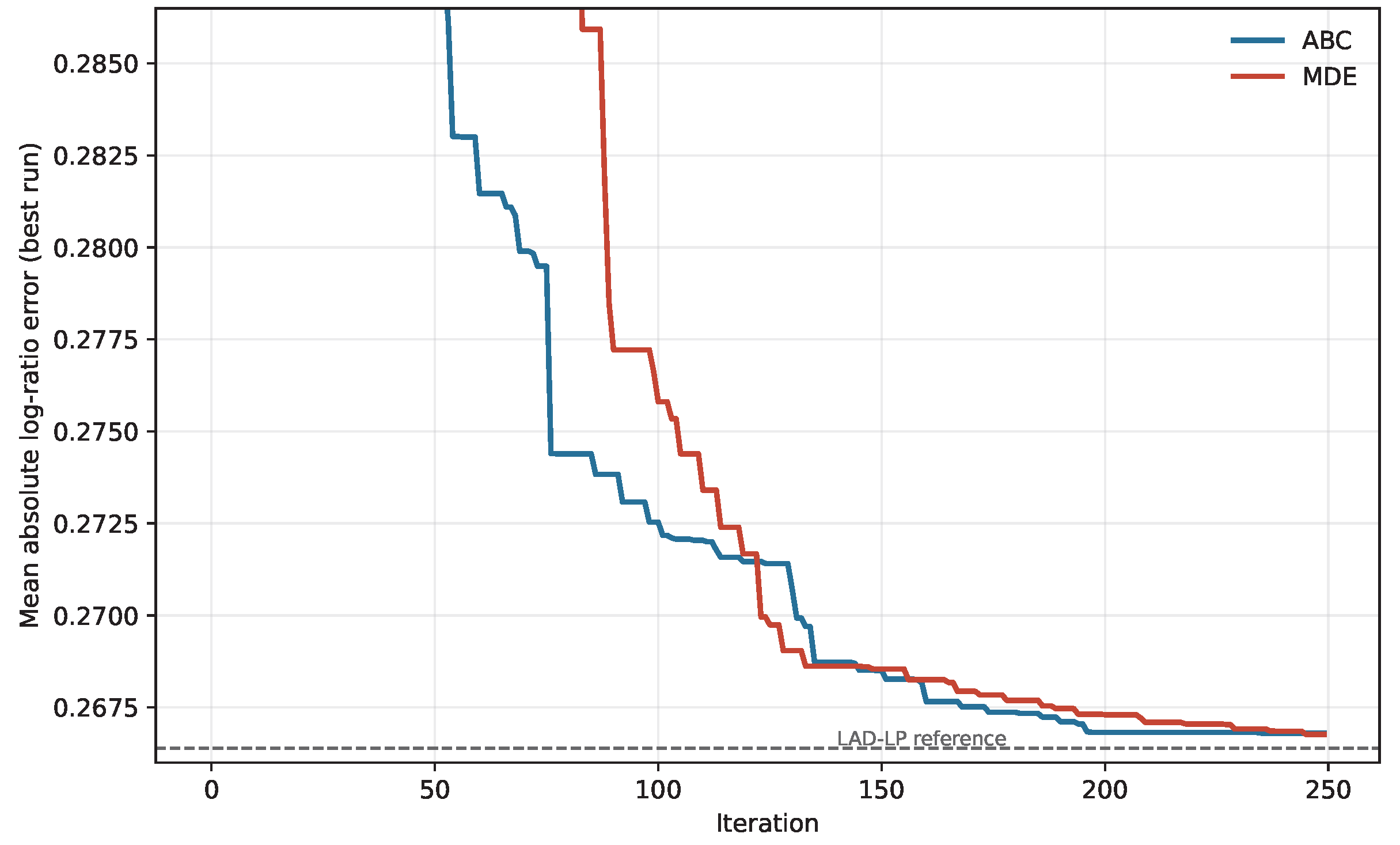
The fitting comparison gives the clearer interpretation. The deterministic least-absolute-deviation program reaches the lowest mean log-ratio error at 0.2664. The best ABC and MDE runs reach 0.2668, logarithmic least squares improves slightly on the eigenvector at 0.2805, and the classical eigenvector sits at 0.2825 (Table 7). All five calibrations preserve the TOPSIS top-ten set. A tractable linear program therefore solves the calibration problem at least as well as either metaheuristic in this case. The evolutionary runs are most useful as an empirical weight ensemble for rank-stability testing. The run-level diagnostics of the two metaheuristics, including their Mann–Whitney comparison and convergence behaviour, are reported in Table A4 and Figure A1.
Table 7.
Deterministic and evolutionary weight-calibration baselines.
The Best-Worst Method offers a reduced-comparison reconstruction from the same consensus judgments. With Transportation as the best and Climatic Conditions as the worst reference criterion, the linear program returns and a Best-Worst consistency ratio of 0.0197. Its weights agree with the eigenvector on the leading groups, and the Best-Worst TOPSIS ranking correlates with the screened AHP ranking at while preserving eight of the top-ten units (Table 8). A model built on only the best and worst reference comparisons therefore reproduces most of the priority structure. This result indicates that the leading units can be recovered from a reduced judgment structure.
Table 8.
Best-Worst Method weights reconstructed from the best and worst reference comparisons of the consensus matrix, and the agreement of the resulting TOPSIS ranking with the screened AHP-TOPSIS ranking.
5.3. Local Inconsistency and Residual Diagnostics
The global consistency ratio understates the local conflict in the matrix. Koczkodaj’s triad indicator is 0.8674, which signals a strong local deviation in at least one triad, and the worst triad couples Physical, Environmental, and Socio-Demographic Characteristics. A high local figure beside a low global one can arise when geometric-mean aggregation combines individually consistent expert matrices that disagree on the ordinal relation among a small set of criteria. The residual diagnostics confirm the same pattern. Calibration lowers the mean and median absolute log-ratio residual, while the maximum residual increases, which means that a single normalised weight vector improves the central fit while leaving some local conflict unresolved (Figure 6). The worst triad matters for decisions because Socio-Demographic Characteristics later shows the largest leave-one-group rank effect. Local inconsistency therefore intersects with rank sensitivity in this case. The full residual summaries, worst triads, and largest pairwise residuals are given in Table A5, Table A6 and Table A7.
Figure 6.
Log-ratio calibration diagnostics. The (left panel) shows absolute residual distributions for the consensus eigenvector and the best evolutionary runs. The (right panel) plots observed log judgments against fitted log ratios for the MDE best run.
5.4. Screened TOPSIS Priority Ranking
TOPSIS on the screened matrix produces a stable leading group. Units 20, 21, 6, 22, and 23 hold the first five positions under classical AHP, ABC, and MDE weights, and units 7, 36, 8, 10, and 9 complete the top ten under all three schemes. The ten highest closeness scores span a narrow band from 0.8210 to 0.8002, and rank 11 follows at 0.7952, leaving a rank-ten to rank-eleven gap of 0.0051 (Table A1 and Figure 7). The top ten should therefore be read as a methodologically stable priority tier under calibrated weights (Figure 8), with a modest cardinal separation from the next unit. The score-threshold values are listed in Appendix A.
Figure 7.
TOPSIS closeness scores for all 54 units under the screened AHP weighting. The top-ten tier and the small rank-ten to rank-eleven gap are marked.
Figure 8.
Rank trajectories of the fifteen highest-priority units under AHP, ABC, and MDE weights. Units are ordered by their screened AHP-TOPSIS rank.
5.5. Judgment Uncertainty from Empirical and Monte Carlo Propagation
Two propagations test how far the leading tier survives uncertainty. The empirical propagation of all 60 evolutionary weight vectors keeps the first five units fixed in ranks one to five and gives the full top-ten group a top-ten frequency of 1.00, with rank movement appearing only below that group (Figure 9). Because each of these vectors is near-optimal under the log-ratio objective, this is a stringent test inside the weight region that the consensus judgments permit.
Figure 9.
Empirical rank ranges of the fifteen highest-priority units across 60 near-optimal ABC and MDE weight vectors. Lower values indicate higher priority.
The Monte Carlo perturbation tests the judgments themselves and gives a sharper diagnosis (Table 9). The same principal-eigenvector estimator is used for the base ranking and for every perturbed matrix, so the noise-free row reproduces the base ranking exactly. At a small noise level of , the top-five overlap is almost always complete and the exact top-five set recurs in 98.5% of simulations. At the mid-scale reference level , the top-five overlap averages 4.76 of five and the top-ten overlap averages 9.70 of ten, while the exact top-five set recurs in 76.0% of 3000 perturbed matrices. Even at , the top-five overlap still averages 4.61 of five.
Table 9.
Monte Carlo robustness of the screened AHP-TOPSIS ranking under lognormal perturbation of the consensus pairwise judgments. Each row aggregates 3000 perturbed matrices; is the standard deviation of the multiplicative judgment noise on the natural-log scale.
The per-unit view in Figure 10 locates the residual instability. Units 20, 21, 6, 22, 23, 7, 36, and 8 hold tight rank intervals with a top-ten frequency of 1.00, and unit 9 stays at the boundary with a frequency of 0.987. Unit 10 behaves differently, ranging from rank 2 to rank 12 across the simulations with a top-ten frequency of only 0.713 (Table A2). The perturbation therefore singles out the same unit that the structural tests later flag, even though the two tests use independent mechanisms.
Figure 10.
Judgment-uncertainty propagation. (A) Average overlap of the top-five and top-ten sets and recurrence of the exact top-five set as the lognormal judgment noise grows, over 3000 perturbed consensus matrices per level. (B) Per-unit rank distributions at the reference level for the twelve highest-priority units, where unit 10 stands out with a wide interval. The dashed line marks the boundary of the top-ten tier.
5.6. Unit Profiles and the GIS Evidence Space
The group-level evidence profiles add information beyond the rank list (Table 10, Figure 11). Units 20, 21, 22, and 23 share high Transportation and Accessibility values near 0.58 to 0.59 with a Physical profile that decreases gradually across the sequence. Unit 6 carries stronger Physical, Environmental, Geological, Energy, and Climatic profiles. Unit 10 stands apart because its single Socio-Demographic profile reaches 1.00. That single high value is exactly what makes unit 10 fragile under the concentration tests.
Table 10.
Evidence profiles and empirical rank stability of the highest-priority independent units. Values in parentheses are benefit–cost normalized group means.
Figure 11.
Benefit–cost normalised group profiles for the fifteen highest-priority units. Values are group means after retained sub-criteria are turned to a common favourable direction.
A two-dimensional PCA ordination of the retained unit profiles shows how the units sit in the high-dimensional evidence space and how the structurally supported core relates to the model-sensitive and lower-priority units (Figure 12). The ordination summarises similarity among units in the screened evidence space, and the structurally supported core occupies a distinct region of that space.
Figure 12.
Evidence-space ordination from PCA of the screened decision matrix. Points are independent units, and colours mark priority classes. Units with almost identical evidence profiles fall on nearly the same coordinates, so some markers of the structurally supported core are partly covered by the symbols drawn over them.
5.7. Benchmark Weighting and Leave-One-Group Sensitivity
The calibrated weights stay close to the classical ranking, with ABC and MDE correlating with AHP at and , and equal main weighting still at (Table 11). The data-driven schemes diverge sharply. Count-adjusted AHP falls to and keeps only four of the top-ten units, equal sub-criterion weighting reaches with five, and entropy and CRITIC fall further still. This divergence follows the column imbalance, because count-adjusted, equal, and dispersion-based weights all shift effective weight toward Accessibility, the group that holds most of the variables (Figure 13, with the full group-weight decomposition in Table A8).
Table 11.
Rank agreement between screened AHP-TOPSIS and alternative weighting schemes.
Figure 13.
Main-criterion weight signatures implied by expert, deterministic, evolutionary, equal, entropy, and CRITIC weighting. Each bar shows the share of total retained sub-criterion weight assigned to each group.
The leave-one-main-criterion-out test confirms that influence does not follow variable count (Table 12, Figure 14). Removing Socio-Demographic Characteristics, a single-variable group, lowers agreement with the base ranking to , shifts ranks by 11.78 positions on average, and changes scores by 0.0778. Removing Physical Characteristics also moves the ranking appreciably. Removing the 203-variable Accessibility group or the 38-variable Transportation group leaves the ordinal ranking unchanged, although the score columns show small score shifts. Energy Management leaves the top-ten set intact yet produces the largest score change of all groups, again because its single variable carries concentrated weight.
Table 12.
Leave-one-main-criterion-out robustness of the screened AHP-TOPSIS ranking.
Figure 14.
Leave-one-main-criterion-out rank agreement with the base screened ranking. A value of 1.000 means the ordinal ranking did not change after removing the group and renormalising.
5.8. Structural, Scoring, and Priority-Core Robustness
The structural checks show that the full matrix and its reduced representations answer related but distinct questions (Table 13, Figure 15). Averaging each retained group into one composite score keeps four of the five leading units and seven to eight of the top ten, but agreement with the full screened model is only moderate. The correlation-clustered model reduces the 284 variables to 56 within-group clusters and raises agreement to , yet it preserves only six of the top-ten units and one of the top five. This appears surprising next to the low effective dimensionality. The explanation lies in the difference between geometric structure in the TOPSIS distance space and a reduced profile summary. Even when many sub-criteria are highly correlated, their combined contribution to ideal-solution distances can differ from a single group or cluster mean. Removing the three single-variable groups reorders the ranking far more, to with one top-five and three top-ten overlaps, which again identifies the concentrated socio-demographic, geological, and energy variables as structurally influential.
Table 13.
Reduced-matrix robustness checks against the screened AHP-TOPSIS ranking.
Figure 15.
Rank agreement between reduced-matrix robustness checks and the base screened AHP-TOPSIS ranking.
Scoring-rule sensitivity points in the same direction. Min–max TOPSIS preserves nine of the top-ten units but lowers agreement to , and simple additive weighting is more disruptive at . The single-variable cap test is the clearest diagnosis of concentration. Capping the effective weight of single-variable groups at ten times the equal weight drops unit 10 to rank 49, and the five- and two-times caps drop it to ranks 50 and 51. The base ranking remains valid as the documented AHP allocation, while unit 10 is marked as a weight-stable yet structure-sensitive case driven by one concentrated socio-demographic indicator. The scoring-rule and single-variable cap summaries are in Table A9 and Table A10.
Combining empirical weight propagation with the seven structural models gives a narrower and more defensible core (Table 14). Units 20, 21, 6, and 22 stay in the top ten under every empirical vector and in at least five of the seven structural models, which places them in the structurally supported core. Units 23, 7, 36, 8, 10, and 9 are stable under calibrated weight variation but miss the structural threshold, so they remain strong field-verification candidates whose standing depends more on modelling assumptions. Unit 10 is the clearest member of this second tier, since the Monte Carlo perturbation and the cap test independently expose its instability.
Table 14.
Priority-core classification combining calibrated weight propagation with structural robustness models.
6. Discussion
The wider significance of these results lies in what they reveal about high-dimensional spatial decision problems rather than in the priority list itself. The central lesson is that the number of criteria is a weak guide to the evidential content of a GIS-MCDA model, because effective dimensionality and effective weight can be strongly shaped by redundancy among correlated layers and by the composition of the criterion hierarchy, not by criterion count. Two theoretical ideas that were developed for aspatial settings, splitting bias in value trees and the gap between nominal and effective weights in composite indicators, are shown here to operate together inside a real unit-level geodatabase, which demonstrates their relevance to spatial valuation support and gives the observed weight concentration a principled explanation rather than an incidental one [29,30,31,32]. The operational distinction between weight sensitivity and structural sensitivity then provides a general way to distinguish findings that remain robust across plausible modelling choices from those that depend more strongly on how the evidence is represented. This distinction is what a GIS-MCDA study can contribute beyond a single ranking.
The analysis should be read as valuation support for pre-transformation review. It orders independent property units through a broad, GIS-derived, expert-weighted evidence system. It does not estimate sale prices, compensation values, or post-transformation entitlements. Professional appraisal still requires market evidence, ownership documentation, field verification, and institutional review [38,39,40]. The value of the workflow lies in making the reasoning behind early prioritisation traceable while keeping the boundary between decision support and monetary appraisal explicit [4,5,6].
Variable screening is the first substantive result. Four conceptually relevant main criteria do not vary across the 54 units in this local matrix, and retaining them as TOPSIS dimensions would have allowed non-discriminating variables to influence the ranking. This finding should be interpreted as a statement about local data resolution. Disaster management, protected areas, waste management, and sustainable living remain important for urban transformation, yet the specific variables available for this neighbourhood do not separate the alternatives once the unit-level matrix is built.
The calibration comparison also clarifies the role of optimisation in this study. The deterministic least-absolute-deviation program reaches the lowest log-ratio error, and logarithmic least squares remains close to the eigenvector solution. The evolutionary calibrators therefore add value mainly as an empirical ensemble for rank-stability testing. They are useful because they generate near-optimal weight vectors compatible with the consensus judgments, which can then be propagated through TOPSIS. The Best-Worst comparison reinforces the same interpretation from a reduced-comparison perspective. A model based on only the best and worst reference comparisons recovers most of the priority order, which indicates that the leading units are not dependent on the full pairwise matrix alone.
The redundancy and concentration diagnostics qualify the strength of the ranking more than any single robustness statistic. A matrix with 284 retained variables appears highly detailed, yet its effective dimensionality is about 2.35, and many proximity and environmental variables move together. Correlated spatial indicators can describe meaningful urban structure, although the matrix cannot be interpreted as 284 independent pieces of evidence. This observation is consistent with previous MCDA research showing that redundant or statistically dependent criteria may repeatedly represent the same latent information and consequently bias the final ranking [10]. Studies on composite indicators similarly emphasise that weighting and aggregation should account for criterion dependence, since nominal weights do not necessarily reflect the effective contribution of variables to the final score [9,20].
The opposite side of this redundancy is weight concentration. Equal within-group allocation gives the single Socio-Demographic, Geological, and Energy variables per-variable weights far above the average. The leave-one-group, no-single-variable, and cap tests show that these concentrated columns govern the sensitive part of the ranking more strongly than the 203-variable Accessibility group. This is the behaviour predicted by the splitting-bias and implicit-weighting literature, in which hierarchy decomposition and unequal group sizes mechanically determine the effective weight received by individual elements once a higher-level weight is distributed within a branch [30,31]. Unit 10 illustrates this mechanism clearly. It is stable under AHP-compatible weight variation, yet it loses its high position when single-variable weights are capped. Its base rank should therefore be treated as a strong but structure-sensitive signal.
The distinction between weight sensitivity and structural sensitivity is the main practical lesson of the results. Under the full screened matrix, calibrated weights move the ranking only slightly, and realistic perturbation of the expert judgments keeps the leading tier largely intact. Under group-composite aggregation, count-adjusted allocation, single-variable caps, min–max TOPSIS, and additive scoring, the broader order changes more substantially. The screened 284-variable ranking is therefore the base expert-weighted configuration. Its stable core can be carried forward with greater confidence, while the wider top-ten tier should be interpreted with the structural diagnostics attached. For practitioners, this means that decisions about how the matrix is represented can matter as much as the choice among AHP-compatible weights [21,23]. These decisions include how many variables belong to each group, whether correlated variables are summarised, and how single-variable groups are handled. This is consistent with recent MCDA research arguing that robustness should be evaluated not only through weight perturbation but also through alternative model structures [12,20].
The final classification gains credibility because independent diagnostics converge. Two types of fragility should be distinguished. The structural-model family identifies units whose top-ten standing depends on how the matrix is aggregated. Unit 36 is an example, since it is stable under calibrated weight variation but leaves the top ten in the seven structural models. Unit 10 is flagged in a different way. The lognormal Monte Carlo perturbation of the judgments, the single-variable cap test, and the leave-one-group test all point to the same unit and trace its sensitivity to one concentrated socio-demographic indicator. A unit that is flagged by several unrelated diagnostics deserves a different level of caution from a unit that is sensitive along one modelling axis. This distinction explains why the study separates a structurally supported core from a weight-stable and structure-sensitive tier rather than relying on a single top-ten list.
The single case study limits external validity. The specific priority list is local to Fatih Neighborhood, while the workflow is transferable as a method. Applying the same screening, calibration, and robustness chain across several transformation neighbourhoods would test whether the separation between a stable core and a model-sensitive tail holds at a wider metropolitan scale. The thematic layers in Figure 2 also show that the evidence base remains spatial even though the final output is reported at the unit level. Future applications could improve the evidence design by widening micro-scale socio-demographic indicators, preserving individual expert matrices for inter-expert analysis, and testing distance or regularisation strategies that remain usable when the covariance matrix is singular.
For planning practice, the framework helps separate stable decisions from sensitive ones. The top-ten tier is invariant under the empirical evolutionary weights and survives realistic judgment noise. The stricter structural-core analysis narrows the most defensible early-priority set to units 20, 21, 6, and 22. The remaining top-ten units still warrant early review, although their relative standing depends more strongly on aggregation and single-variable assumptions. The empirical and Monte Carlo rank ranges can guide the intensity of field verification, and the diagnostics can guide data improvement by showing which groups are non-discriminating, redundant, or overly concentrated. This reflects the broader position that a decision-support system should report not only a ranking but also the model assumptions, uncertainty, and robustness behind it, which is what makes a planning recommendation interpretable and open to challenge [8].
For an urban renewal programme operating under time and budget constraints, this has direct practical value: it indicates where scarce field and appraisal effort is best directed and where a high-ranked unit should be treated with caution, thereby reducing the risk of committing resources on the basis of a ranking that modest changes in modelling assumptions could overturn. This transparency matters beyond efficiency. Prioritisation in dense urban renewal is embedded in wider processes involving compensation, relocation, and perceptions of fairness, and reporting which parts of a ranking are robust and which depend on modelling choices therefore gives planners and affected parties a clearer basis for examining and, where necessary, revising the order of field review, rather than treating the model output as a single authoritative decision. In this sense the diagnostic outputs support not only more efficient verification but also more accountable and defensible prioritisation, which is where much of the practical difficulty in urban transformation actually lies.
7. Conclusions
Urban transformation decisions carry long consequences for residents, owners, and public institutions. A valuation-support workflow should therefore make clear which criteria actually separate units, where expert judgment is consistent or conflicted, and how modelling choices move the priority order. This study developed a reproducible GIS-MCDA workflow for 54 independent property units in Fatih Neighborhood, Esenler District, Istanbul. The workflow screened a 311-indicator geodatabase to 284 locally discriminating variables and then linked expert weighting, TOPSIS ranking, uncertainty propagation, redundancy diagnosis, and structural robustness testing in a single analysis chain.
Three conclusions follow from the results. First, the apparent richness of a high-dimensional urban database can mask strong redundancy and uneven effective weighting. The screened matrix contains 284 retained variables, yet much of its variance is concentrated in a small number of shared spatial directions, and single-variable groups receive concentrated per-variable influence under equal within-group allocation. Second, the leading priority tier is stable under calibrated weight variation and realistic judgment noise, while the wider ordering is much more sensitive to matrix structure, within-group aggregation, single-variable groups, and scoring rule. Third, combining weight propagation with structural robustness produces a defensible early-verification core. In this case, units 20, 21, 6, and 22 form that core. The other high-ranking units remain relevant for early review, with their standing reported as more model-dependent.
The methodological contribution lies in turning a ranking exercise into an auditable diagnostic chain. The workflow reports non-discriminating criteria, effective sub-criterion weights, local inconsistency, calibration residuals, redundancy, benchmark divergence, judgment-noise propagation, structural robustness, and unit-level evidence profiles. These outputs support professional valuation judgment by showing where the ranking is stable and where more field, market, or institutional evidence is needed. The broader significance is a transferable way of reading high-dimensional spatial decision problems, in which the credibility of a ranking rests not on the size of its evidence base but on how much of that evidence is independent and on how far its structure is allowed to shape the result.
The framework is intended to help prioritise field verification and appraisal work, not to replace conventional valuation procedures. Although it is demonstrated in a single urban renewal area, its behaviour was examined under multiple weighting, optimisation, benchmarking, and uncertainty scenarios, which provides a basis for application in other transformation contexts. What the analysis establishes is the robustness of the resulting rankings rather than their real-world accuracy, because independent evidence such as expert review, field verification, or realised redevelopment priorities was not available within the scope of the study. External validation against such evidence is therefore the most important direction for future research, together with preserving individual expert matrices for inter-expert disagreement analysis, expanding unit-level socio-demographic evidence, testing covariance-regularised or correlation-aware distance metrics, and applying the workflow across multiple transformation neighbourhoods.
Author Contributions
Conceptualization, Ö.Ö., A.B. and A.E.K.; methodology, Ö.Ö., A.B., A.E.K. and F.E.; software, Ö.Ö., A.E.K. and R.A.K.; validation, A.B., A.E.K., T.Y. and R.A.K.; formal analysis, Ö.Ö. and A.E.K.; investigation, Ö.Ö., A.B., M.H. and F.E.; resources, A.B., M.H. and T.Y.; data curation, Ö.Ö. and R.A.K.; writing—original draft preparation, Ö.Ö., A.B. and A.E.K.; writing—review and editing, A.B., A.E.K., M.H., F.E., T.Y., R.A.K. and Z.Ü.; visualization, Ö.Ö., A.E.K., M.H. and R.A.K.; supervision, A.B., F.E. and T.Y.; project administration, A.B.; funding acquisition, A.B. All authors have read and agreed to the published version of the manuscript.
Funding
This research was carried out within the scope of TÜBİTAK 1001 project number 323K226. The APC was funded by the authors.
Institutional Review Board Statement
The study was conducted in accordance with the Declaration of Helsinki and approved by the Ethics Committee of Niğde Ömer Halisdemir University (meeting dated 30 July 2025, no. 14; decision no. 2025/14-50). The study also complies with the RESPECT Code of Practice for Socio-Economic Research, the principles of the Committee on Publication Ethics (COPE), and the Directive on Scientific Research and Publication Ethics of Higher Education Institutions.
Informed Consent Statement
Informed consent was obtained from all experts who took part in the pairwise comparison survey.
Data Availability Statement
The analysis code that reproduces the variable screening, weight calibration, ranking, and robustness diagnostics is openly available under the MIT License at https://github.com/Aekarkinli/GIS-MCDA-Pipeline-for-Urban-Transformation-Priority-Assessment.git (accessed on 6 August 2026). The data that support the findings of this study are available from the corresponding author upon reasonable request.
Acknowledgments
The authors would like to thank TÜBİTAK for its support and valuable contribution to the realisation of this research under TÜBİTAK 1001 project number 323K226, and Esenler Municipality for its valuable support, cooperation, and feedback during the pilot implementation and user evaluation processes of the project. During the preparation of this manuscript, the authors used the generative artificial intelligence tools Claude (Anthropic) and ChatGPT (OpenAI) solely to check the English language and to improve clarity of expression. The authors reviewed and edited the resulting text and take full responsibility for the content of the publication. No generative artificial intelligence tool was used for the study design, data collection, analysis, interpretation of the results, or the generation of scientific content.
Conflicts of Interest
The authors declare no conflicts of interest.
Appendix A. Diagnostic and Structural Robustness Tables
The tables below carry the numerical detail behind the main findings and each is referenced individually from Section 5 and Section 6. They report the score thresholds that define the top-ten tier, the Monte Carlo rank intervals summarised in Section 5.5, the parameter settings and run-level optimisation diagnostics needed to reproduce the evolutionary calibration, the log-ratio residual and local inconsistency summaries behind the AHP diagnostics, the benchmark weight distributions underlying the rank-agreement comparisons, and the normalisation, scoring, and single-variable cap tests that support the structural robustness analysis. None of this detail is reproduced in the main text.
Table A1.
Score-threshold diagnostics for the screened AHP-TOPSIS ranking.
Table A2.
Monte Carlo rank intervals for the highest-priority units at the reference perturbation level (3000 perturbed matrices).
Table A3.
Parameter settings and implementation details for the evolutionary calibration runs.
Table A4.
Optimization diagnostics for the consensus pairwise comparison matrix.
Table A5.
Log-ratio residual diagnostics for the consensus AHP matrix.
Table A6.
Largest local triadic inconsistencies in the consensus pairwise comparison matrix. Index is Koczkodaj’s triad indicator. Ratio is ; values away from 1 indicate local multiplicative inconsistency.
Table A7.
Largest pairwise log-ratio residuals after MDE best-run calibration.
Table A8.
Main-criterion weight concentration implied by benchmark weighting schemes.
Table A9.
Sensitivity of the screened AHP ranking to TOPSIS normalization and additive scoring.
Table A10.
Sensitivity to capping the effective weight of single-variable main-criterion groups.
Figure A1.
Best-run convergence of the ABC and MDE calibrations under the mean absolute log-ratio objective. The dashed line marks the deterministic least-absolute-deviation reference.
Appendix B. Evolutionary Calibration Operators
This appendix records the operator definitions of the two evolutionary calibrators applied in Section 4.3. Both operate on positive 14-dimensional vectors bounded between and , and every candidate is normalised to a weight vector before the common log-ratio objective F is evaluated. The parameter settings used in the reported runs are listed in Table A3.
For the Artificial Bee Colony calibration, initial food-source positions are sampled uniformly,
The employed and onlooker phases then perturb a single random component around another food source,
while the remaining components stay unchanged [54].
For the multi-population differential evolution calibration, two distinct working indices r and s are drawn for a working target , and the temporary mutant is
where is drawn from , is drawn from , and is the current best candidate. The internal scale term is
with , , , , and . A stochastic binary mask controls crossover without a fixed crossover rate, and the trial vector is
with a small diversity term
References
- Roberts, P.; Sykes, H. (Eds.) Urban Regeneration: A Handbook; SAGE Publications: London, UK, 2000. [Google Scholar]
- Adair, A.; Hutchison, N.; Burgess, J.; Roulac, S. The appraisal of urban regeneration land: A contemporary perspective. J. Prop. Invest. Financ. 2005, 23, 213–233. [Google Scholar] [CrossRef] [Scilit]
- Jankowski, P. Integrating geographical information systems and multiple criteria decision-making methods. Int. J. Geogr. Inf. Syst. 1995, 9, 251–273. [Google Scholar] [CrossRef] [Scilit]
- Malczewski, J. GIS-based multicriteria decision analysis: A survey of the literature. Int. J. Geogr. Inf. Sci. 2006, 20, 703–726. [Google Scholar] [CrossRef] [Scilit]
- Greene, R.; Devillers, R.; Luther, J.E.; Eddy, B.G. GIS-based multiple-criteria decision analysis. Geogr. Compass 2011, 5, 412–432. [Google Scholar] [CrossRef] [Scilit]
- Malczewski, J.; Rinner, C. Multicriteria Decision Analysis in Geographic Information Science; Springer: Berlin/Heidelberg, Germany, 2015. [Google Scholar] [CrossRef] [Scilit]
- Goyal, P.; Kumar, D.; Kumar, V. Application of multi-criteria decision analysis in the area of sustainability: A literature review. Int. J. Anal. Hierarchy Process 2020, 12, 512–545. [Google Scholar] [CrossRef] [Scilit]
- Cinelli, M.; Kadziński, M.; Gonzalez, M.; Słowiński, R. How to support the application of multiple criteria decision analysis? Let us start with a comprehensive taxonomy. Omega 2020, 96, 102261. [Google Scholar] [CrossRef] [Scilit] [PubMed]
- El Gibari, S.; Gómez, T.; Ruiz, F. Building composite indicators using multicriteria methods: A review. J. Bus. Econ. 2019, 89, 1–24. [Google Scholar] [CrossRef] [Scilit]
- Pelegrina, G.D.; Duarte, L.T.; Grabisch, M.; Romano, J.M.T. Dealing with redundancies among criteria in multicriteria decision making through independent component analysis. Comput. Ind. Eng. 2022, 169, 108171. [Google Scholar] [CrossRef] [Scilit]
- de Farias Aires, R.F.; Ferreira, L. The rank reversal problem in multi-criteria decision making: A literature review. Pesqui. Oper. 2018, 38, 331–362. [Google Scholar] [CrossRef] [Scilit]
- Zandi, I.; Pahlavani, P.; Bigdeli, B.; Lotfata, A.; Alesheikh, A.A.; Garau, C. GIS-enabled multi-criteria assessment for hospital site suitability: A case study of Tehran. Sustainability 2024, 16, 2079. [Google Scholar] [CrossRef] [Scilit]
- Rad, M.; Sonesson, U.; Höglund, E.; Östergren, K. Multi-criteria decision analysis (MCDA) for sustainability assessment: How reliable are the results? Sustain. Futures 2026, 11, 101657. [Google Scholar] [CrossRef] [Scilit]
- O’Shea, R.; Deeney, P.; Triantaphyllou, E.; Diaz-Balteiro, L.; Tarim, S.A. Weight stability intervals for multi-criteria decision analysis using the weighted sum model. Expert Syst. Appl. 2026, 296, 128460. [Google Scholar] [CrossRef] [Scilit]
- Kuyucu, T.; Ünsal, Ö. Urban transformation as state-led property transfer: An analysis of two cases of urban renewal in Istanbul. Urban Stud. 2010, 47, 1479–1499. [Google Scholar] [CrossRef] [Scilit]
- Karaman, O. Urban renewal in Istanbul: Reconfigured spaces, robotic lives. Int. J. Urban Reg. Res. 2013, 37, 715–733. [Google Scholar] [CrossRef] [Scilit]
- Kuyucu, T. Politics of urban regeneration in Turkey: Possibilities and limits of municipal regeneration initiatives in a highly centralized country. Urban Geogr. 2018, 39, 1152–1176. [Google Scholar] [CrossRef] [Scilit]
- Binici, B.; Yakut, A.; Ozcebe, G.; Erenler, A. Provisions for the seismic risk evaluation of existing reinforced concrete buildings in Turkey under the urban renewal law. Earthq. Spectra 2015, 31, 1413–1433. [Google Scholar] [CrossRef] [Scilit]
- Jiang, H.; Eastman, J.R. Application of fuzzy measures in multi-criteria evaluation in GIS. Int. J. Geogr. Inf. Sci. 2000, 14, 173–184. [Google Scholar] [CrossRef] [Scilit]
- Greco, S.; Ishizaka, A.; Tasiou, M.; Torrisi, G. On the methodological framework of composite indices: A review of the issues of weighting, aggregation, and robustness. Soc. Indic. Res. 2019, 141, 61–94. [Google Scholar] [CrossRef] [Scilit]
- Feizizadeh, B.; Jankowski, P.; Blaschke, T. A GIS based spatially-explicit sensitivity and uncertainty analysis approach for multi-criteria decision analysis. Comput. Geosci. 2014, 64, 81–95. [Google Scholar] [CrossRef] [Scilit] [PubMed]
- Erlacher, C.; Anders, K.H.; Jankowski, P.; Paulus, G.; Blaschke, T. A Framework for Cloud-Based Spatially-Explicit Uncertainty and Sensitivity Analysis in Spatial Multi-Criteria Models. ISPRS Int. J. Geo-Inf. 2021, 10, 244. [Google Scholar] [CrossRef] [Scilit]
- Więckowski, J.; Sałabun, W. Sensitivity analysis approaches in multi-criteria decision analysis: A systematic review. Appl. Soft Comput. 2023, 148, 110915. [Google Scholar] [CrossRef] [Scilit]
- Nardo, M.; Saisana, M.; Saltelli, A.; Tarantola, S.; Hoffman, A.; Giovannini, E. Handbook on Constructing Composite Indicators: Methodology and User Guide; OECD Publishing: Paris, France, 2008. [Google Scholar] [CrossRef] [Scilit]
- Rahman, M.M.; Szabó, G. Sustainable urban land-use optimization using GIS-based multicriteria decision-making (GIS-MCDM) approach. ISPRS Int. J. Geo-Inf. 2022, 11, 313. [Google Scholar] [CrossRef] [Scilit]
- Foroozesh, F.; Monavari, S.M.; Salmanmahiny, A.; Robati, M.; Rahimi, R. Assessment of sustainable urban development based on a hybrid decision-making approach: Group fuzzy BWM, AHP, and TOPSIS-GIS. Sustain. Cities Soc. 2022, 76, 103402. [Google Scholar] [CrossRef] [Scilit]
- Zhao, L.Q.; van Duynhoven, A.; Dragićević, S. Machine learning for criteria weighting in GIS-based multi-criteria evaluation: A case study of urban suitability analysis. Land 2024, 13, 1288. [Google Scholar] [CrossRef] [Scilit]
- Zhao, L.Q.; Dragićević, S. Assessing the number of criteria in GIS-based multicriteria evaluation: A machine learning approach. Geogr. Anal. 2025, 57, 489–506. [Google Scholar] [CrossRef] [Scilit]
- Stillwell, W.G.; von Winterfeldt, D.; John, R.S. Comparing hierarchical and nonhierarchical weighting methods for eliciting multiattribute value models. Manag. Sci. 1987, 33, 442–450. [Google Scholar] [CrossRef] [Scilit]
- Weber, M.; Eisenführ, F.; von Winterfeldt, D. The effects of splitting attributes on weights in multiattribute utility measurement. Manag. Sci. 1988, 34, 431–445. [Google Scholar] [CrossRef] [Scilit]
- Paruolo, P.; Saisana, M.; Saltelli, A. Ratings and rankings: Voodoo or science? J. R. Stat. Soc. Ser. A (Stat. Soc.) 2013, 176, 609–634. [Google Scholar]
- Becker, W.; Saisana, M.; Paruolo, P.; Vandecasteele, I. Weights and importance in composite indicators: Closing the gap. Ecol. Indic. 2017, 80, 12–22. [Google Scholar] [CrossRef] [Scilit] [PubMed]
- Omidipoor, M.; Jelokhani-Niaraki, M.; Moeinmehr, A.; Sadeghi-Niaraki, A.; Choi, S.M. A GIS-based decision support system for facilitating participatory urban renewal process. Land Use Policy 2019, 88, 104150. [Google Scholar] [CrossRef] [Scilit]
- Zhu, S.; Li, D.; Feng, H.; Gu, T.; Zhu, J. AHP-TOPSIS-based evaluation of the relative performance of multiple neighborhood renewal projects: A case study in Nanjing, China. Sustainability 2019, 11, 4545. [Google Scholar] [CrossRef] [Scilit]
- Lin, S.H.; Huang, X.; Fu, G.; Chen, J.T.; Zhao, X.; Li, J.H.; Tzeng, G.H. Evaluating the sustainability of urban renewal projects based on a model of hybrid multiple-attribute decision-making. Land Use Policy 2021, 108, 105570. [Google Scholar] [CrossRef] [Scilit]
- Zhao, P.; Md Ali, Z.; Ahmad, Y. Developing indicators for sustainable urban regeneration in historic urban areas: Delphi method and Analytic Hierarchy Process. Sustain. Cities Soc. 2023, 99, 104990. [Google Scholar] [CrossRef] [Scilit]
- Deng, Y.; Tang, Z.; Liu, B.; Shi, Y.; Deng, M.; Liu, E. Renovation and reconstruction of urban land use by a cost-heuristic genetic algorithm: A case in Shenzhen. ISPRS Int. J. Geo-Inf. 2024, 13, 250. [Google Scholar] [CrossRef] [Scilit]
- Wyatt, P.J. The development of a GIS-based property information system for real estate valuation. Int. J. Geogr. Inf. Sci. 1997, 11, 435–450. [Google Scholar] [CrossRef] [Scilit]
- Wang, D.; Li, V.J. Mass Appraisal Models of Real Estate in the 21st Century: A Systematic Literature Review. Sustainability 2019, 11, 7006. [Google Scholar] [CrossRef] [Scilit]
- Droj, G.; Kwartnik-Pruc, A.; Droj, L. A comprehensive overview regarding the impact of GIS on property valuation. ISPRS Int. J. Geo-Inf. 2024, 13, 175. [Google Scholar] [CrossRef] [Scilit]
- Ayalke, Z.; Sisman, A. Nominal land valuation with best-worst method using geographic information system: A case of Atakum, Samsun. ISPRS Int. J. Geo-Inf. 2022, 11, 213. [Google Scholar] [CrossRef] [Scilit]
- Saaty, T.L. The Analytic Hierarchy Process; McGraw-Hill: New York, NY, USA, 1980. [Google Scholar]
- Saaty, T.L. Decision making with the analytic hierarchy process. Int. J. Serv. Sci. 2008, 1, 83–98. [Google Scholar] [CrossRef] [Scilit]
- Aczél, J.; Saaty, T.L. Procedures for synthesizing ratio judgements. J. Math. Psychol. 1983, 27, 93–102. [Google Scholar] [CrossRef] [Scilit]
- Forman, E.; Peniwati, K. Aggregating individual judgments and priorities with the analytic hierarchy process. Eur. J. Oper. Res. 1998, 108, 165–169. [Google Scholar] [CrossRef] [Scilit]
- Crawford, G.; Williams, C. A note on the analysis of subjective judgment matrices. J. Math. Psychol. 1985, 29, 387–405. [Google Scholar] [CrossRef] [Scilit]
- Aguarón, J.; Moreno-Jiménez, J.M. The geometric consistency index: Approximated thresholds. Eur. J. Oper. Res. 2003, 147, 137–145. [Google Scholar] [CrossRef] [Scilit]
- Koczkodaj, W.W.; Szwarc, R. On axiomatization of inconsistency indicators for pairwise comparisons. Fundam. Informaticae 2014, 132, 485–500. [Google Scholar] [CrossRef] [Scilit]
- Aguarón, J.; Escobar, M.T.; Moreno-Jiménez, J.M.; Turón, A. The Triads Geometric Consistency Index in AHP-Pairwise Comparison Matrices. Mathematics 2020, 8, 926. [Google Scholar] [CrossRef] [Scilit]
- Zhang, J.; Kou, G.; Peng, Y.; Zhang, Y. Estimating priorities from relative deviations in pairwise comparison matrices. Inf. Sci. 2021, 552, 310–327. [Google Scholar] [CrossRef] [Scilit]
- Rezaei, J. Best-worst multi-criteria decision-making method. Omega 2015, 53, 49–57. [Google Scholar] [CrossRef] [Scilit]
- Rezaei, J. Best-worst multi-criteria decision-making method: Some properties and a linear model. Omega 2016, 64, 126–130. [Google Scholar] [CrossRef] [Scilit]
- Saaty, T.L.; Vargas, L.G. Uncertainty and rank order in the analytic hierarchy process. Eur. J. Oper. Res. 1987, 32, 107–117. [Google Scholar] [CrossRef] [Scilit]
- Karaboga, D.; Basturk, B. A powerful and efficient algorithm for numerical function optimization: Artificial Bee Colony algorithm. J. Glob. Optim. 2007, 39, 459–471. [Google Scholar] [CrossRef] [Scilit]
- Karaboga, D.; Basturk, B. On the performance of Artificial Bee Colony algorithm. Appl. Soft Comput. 2008, 8, 687–697. [Google Scholar] [CrossRef] [Scilit]
- Storn, R.; Price, K. Differential evolution: A simple and efficient heuristic for global optimization over continuous spaces. J. Glob. Optim. 1997, 11, 341–359. [Google Scholar] [CrossRef] [Scilit]
- Renigier-Biłozor, M.; Chmielewska, A.; Walacik, M.; Janowski, A.; Lepkova, N. Genetic algorithm application for real estate market analysis in the uncertainty conditions. J. Hous. Built Environ. 2021, 36, 1629–1670. [Google Scholar] [CrossRef] [Scilit]
- Karkinli, A.E. Detection of object boundary from point cloud by using multi-population based differential evolution algorithm. Neural Comput. Appl. 2023, 35, 5193–5206. [Google Scholar] [CrossRef] [Scilit]
- Hwang, C.L.; Yoon, K. Multiple Attribute Decision Making: Methods and Applications; Springer: Berlin/Heidelberg, Germany, 1981. [Google Scholar] [CrossRef] [Scilit]
- Opricovic, S.; Tzeng, G.H. Compromise solution by MCDM methods: A comparative analysis of VIKOR and TOPSIS. Eur. J. Oper. Res. 2004, 156, 445–455. [Google Scholar] [CrossRef] [Scilit]
- Ciardiello, F.; Genovese, A. A comparison between TOPSIS and SAW methods. Ann. Oper. Res. 2023, 325, 967–994. [Google Scholar] [CrossRef] [Scilit]
- Shyur, H.J.; Shih, H.S. Resolving Rank Reversal in TOPSIS: A Comprehensive Analysis of Distance Metrics and Normalization Methods. Informatica 2024, 35, 837–858. [Google Scholar] [CrossRef] [Scilit]
- Shannon, C.E. A mathematical theory of communication. Bell Syst. Tech. J. 1948, 27, 379–423. [Google Scholar] [CrossRef] [Scilit]
- Diakoulaki, D.; Mavrotas, G.; Papayannakis, L. Determining objective weights in multiple criteria problems: The CRITIC method. Comput. Oper. Res. 1995, 22, 763–770. [Google Scholar] [CrossRef] [Scilit]
- Xavier, A.; Fragoso, R.; Costa Freitas, M.d.B. Building sustainability composite indicators using a multi-criteria approach. Eur. J. Oper. Res. 2025, 326, 326–342. [Google Scholar] [CrossRef] [Scilit]
- Wen, T.; Li, P. Spatial Decision Support Systems with Automated Machine Learning: A Review. ISPRS Int. J. Geo-Inf. 2023, 12, 12. [Google Scholar] [CrossRef] [Scilit]
- Melillo, P.; Pecchia, L. What is the appropriate sample size to run analytic hierarchy process in a survey-based research? In Proceedings of the International Symposium on the Analytic Hierarchy Process (ISAHP), London, UK, 4–7 August 2016; pp. 4–8. [Google Scholar] [CrossRef] [Scilit]
- Kil, S.H.; Lee, D.K.; Kim, J.H.; Li, M.H.; Newman, G. Utilizing the analytic hierarchy process to establish weighted values for evaluating the stability of slope revegetation based on hydroseeding applications in South Korea. Sustainability 2016, 8, 58. [Google Scholar] [CrossRef] [Scilit]
- Guillén-Mena, V.; Quesada-Molina, F.; Astudillo-Cordero, S.; Lema, M.; Ortiz-Fernández, J. Lessons learned from a study based on the AHP method for the assessment of sustainability in neighborhoods. MethodsX 2023, 11, 102440. [Google Scholar] [CrossRef] [Scilit] [PubMed]
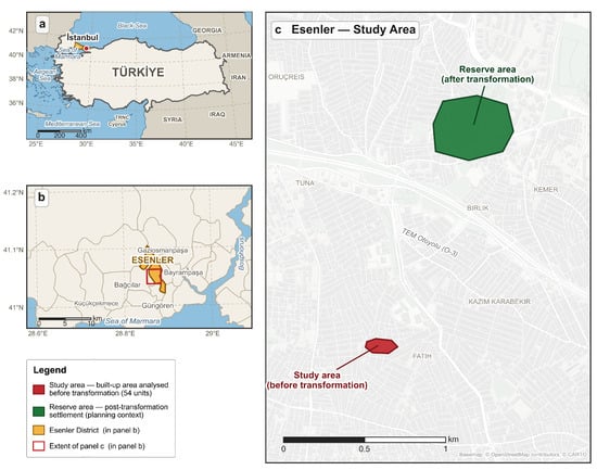
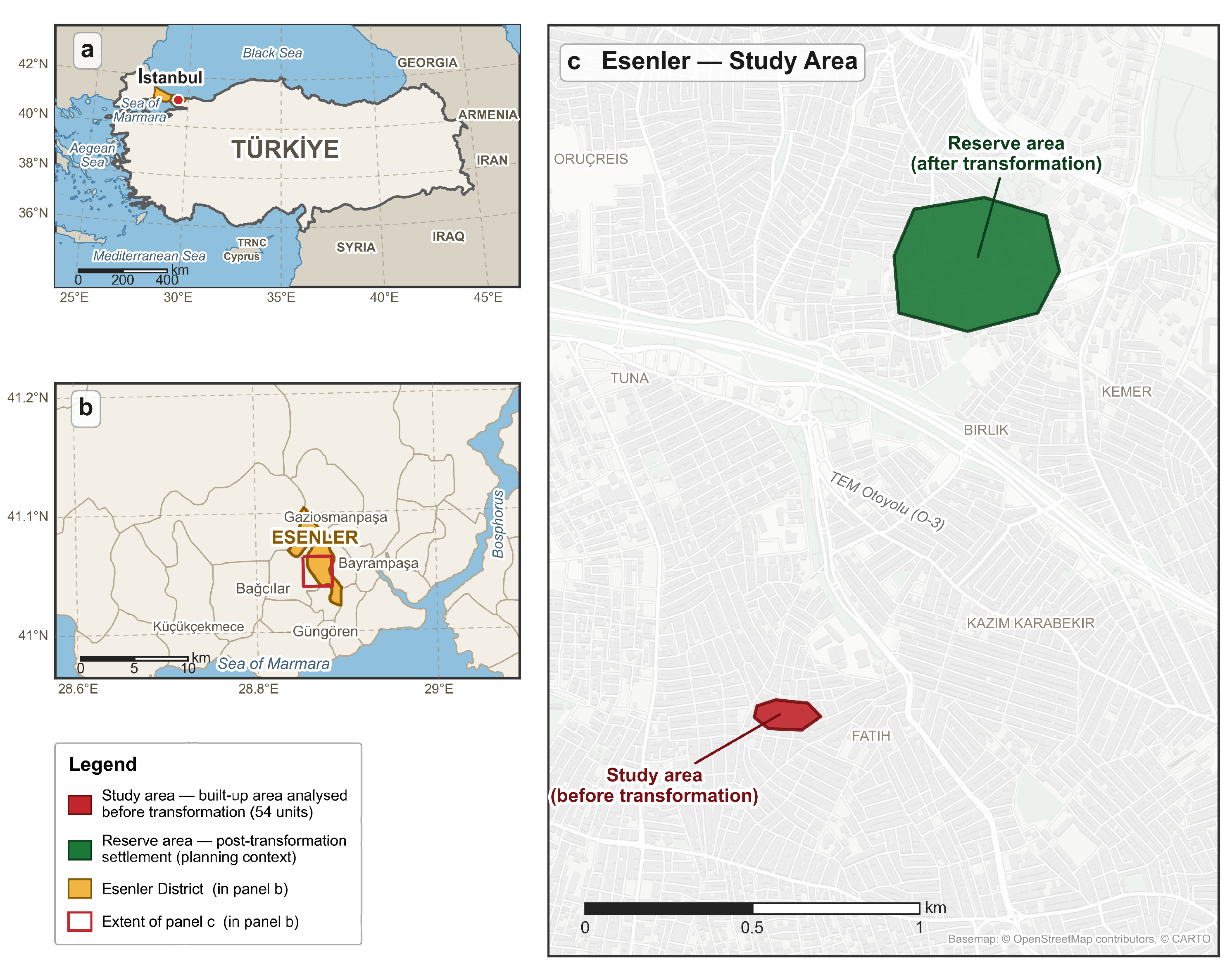
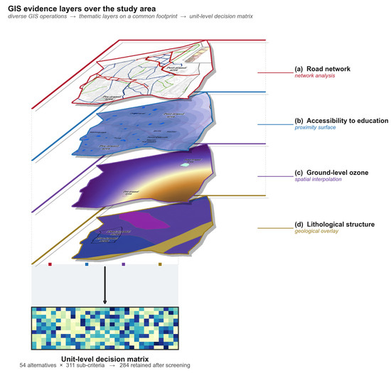
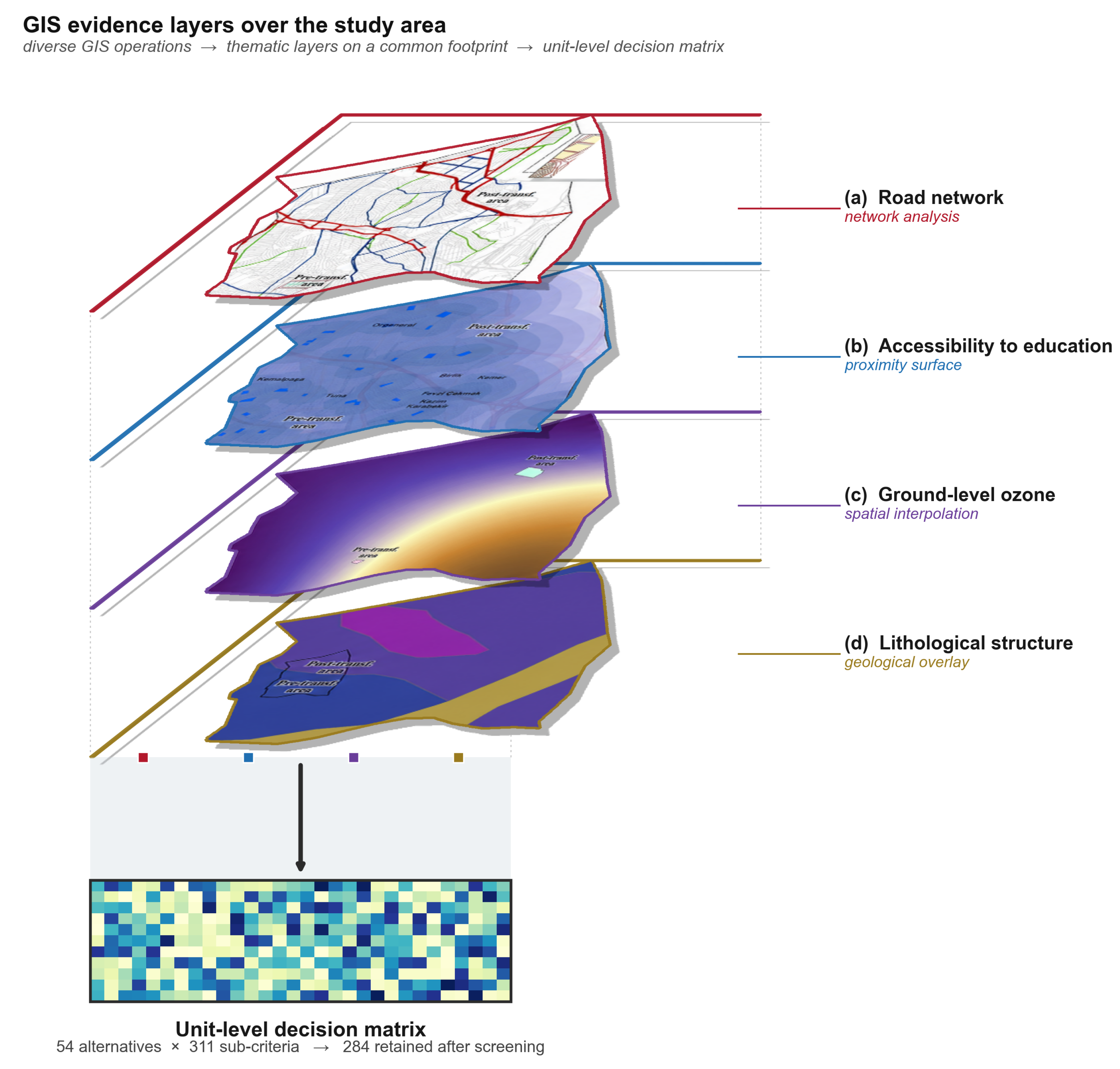
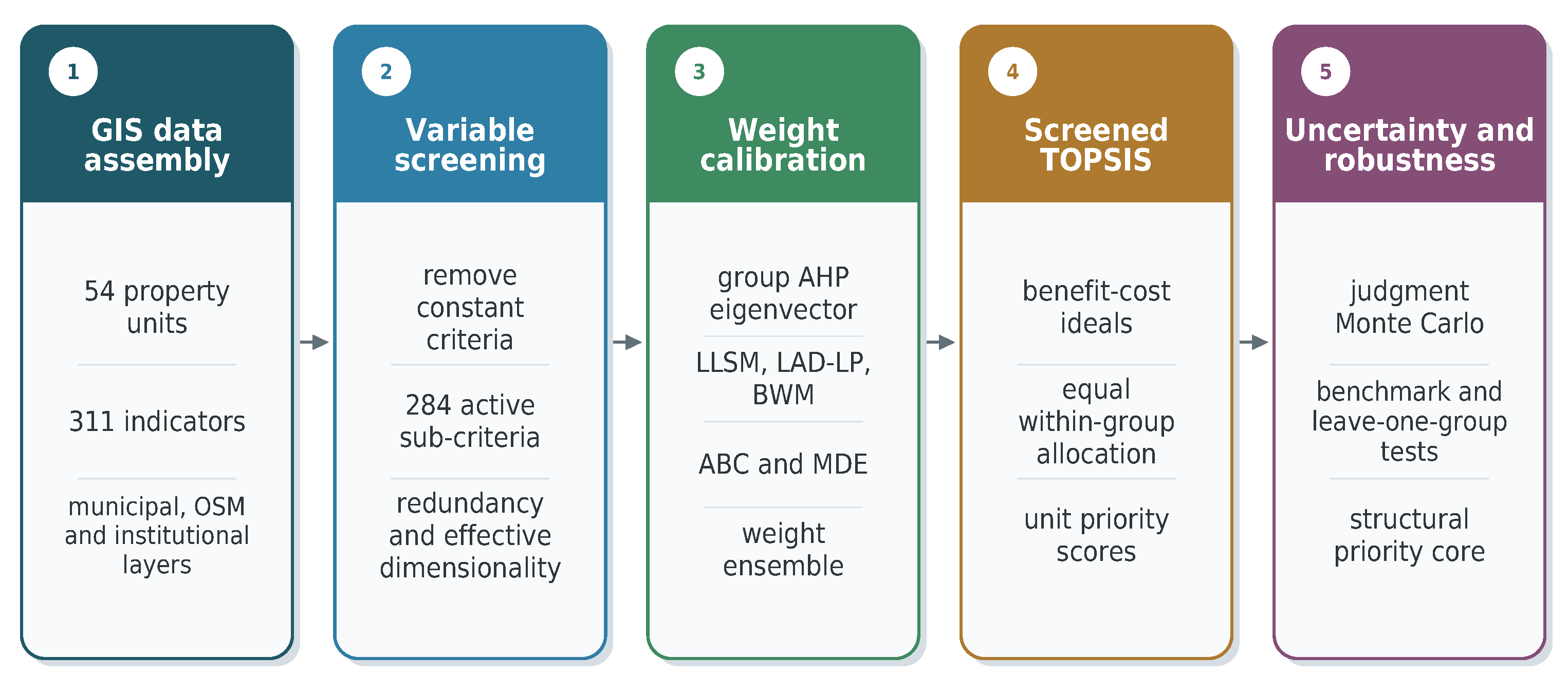
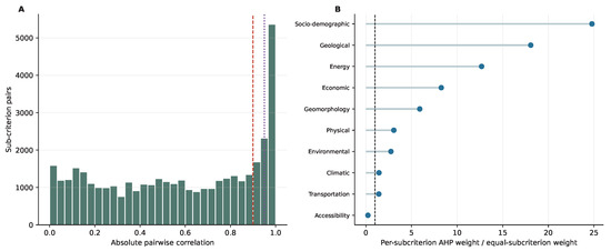
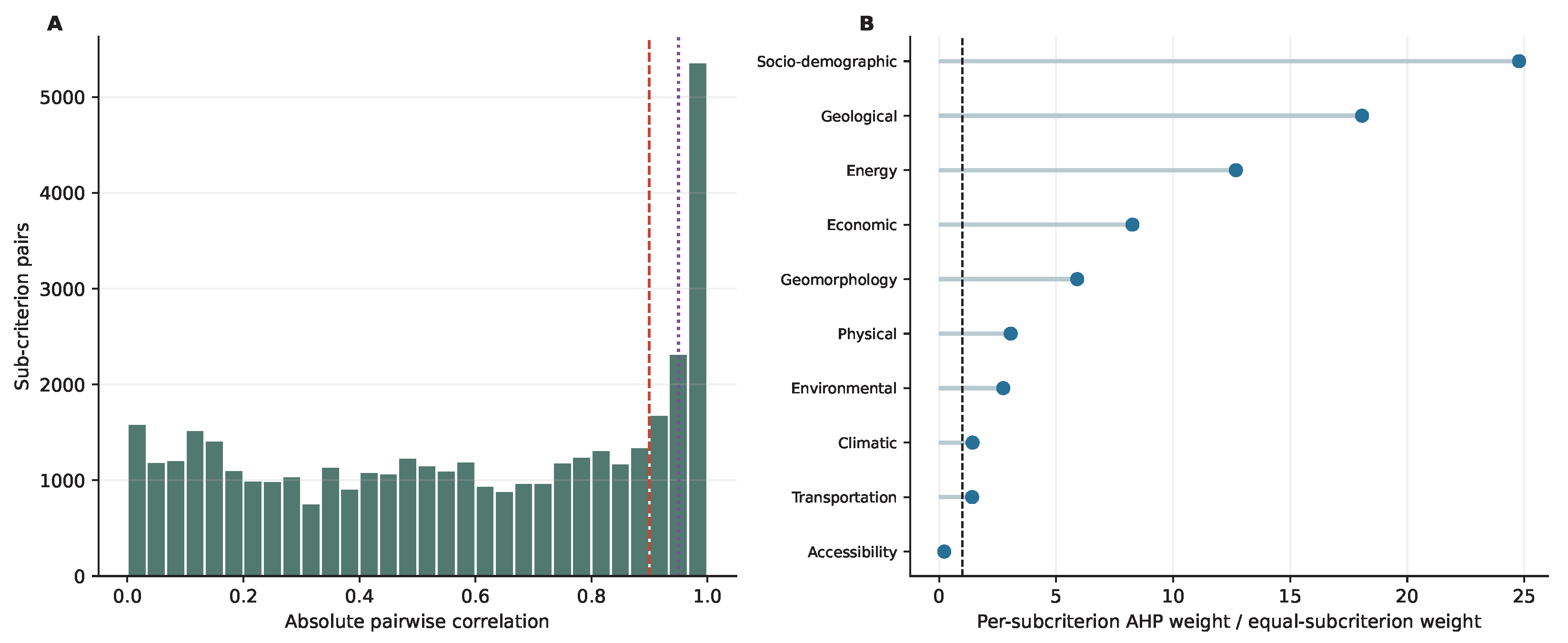
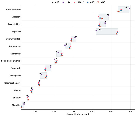
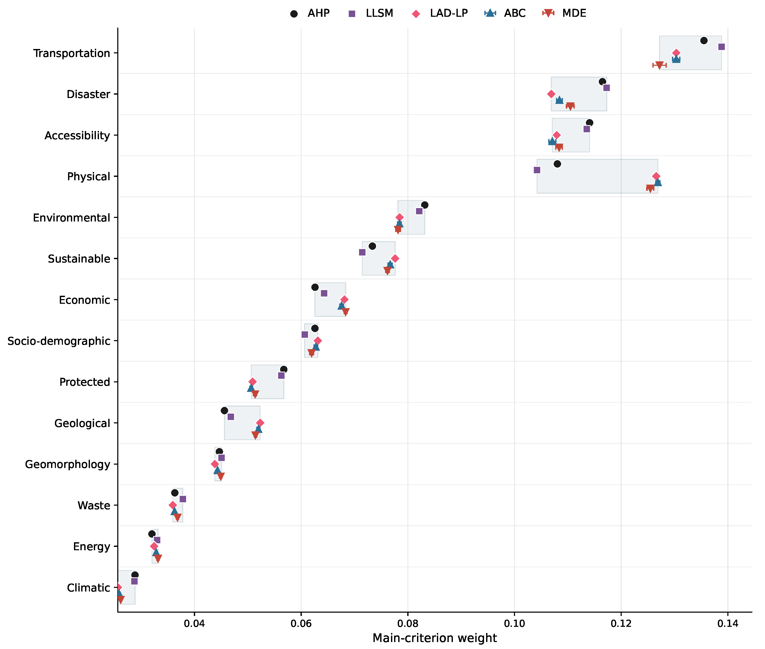
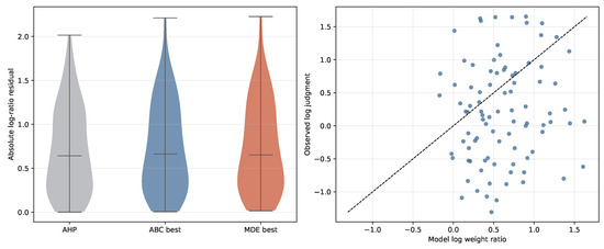
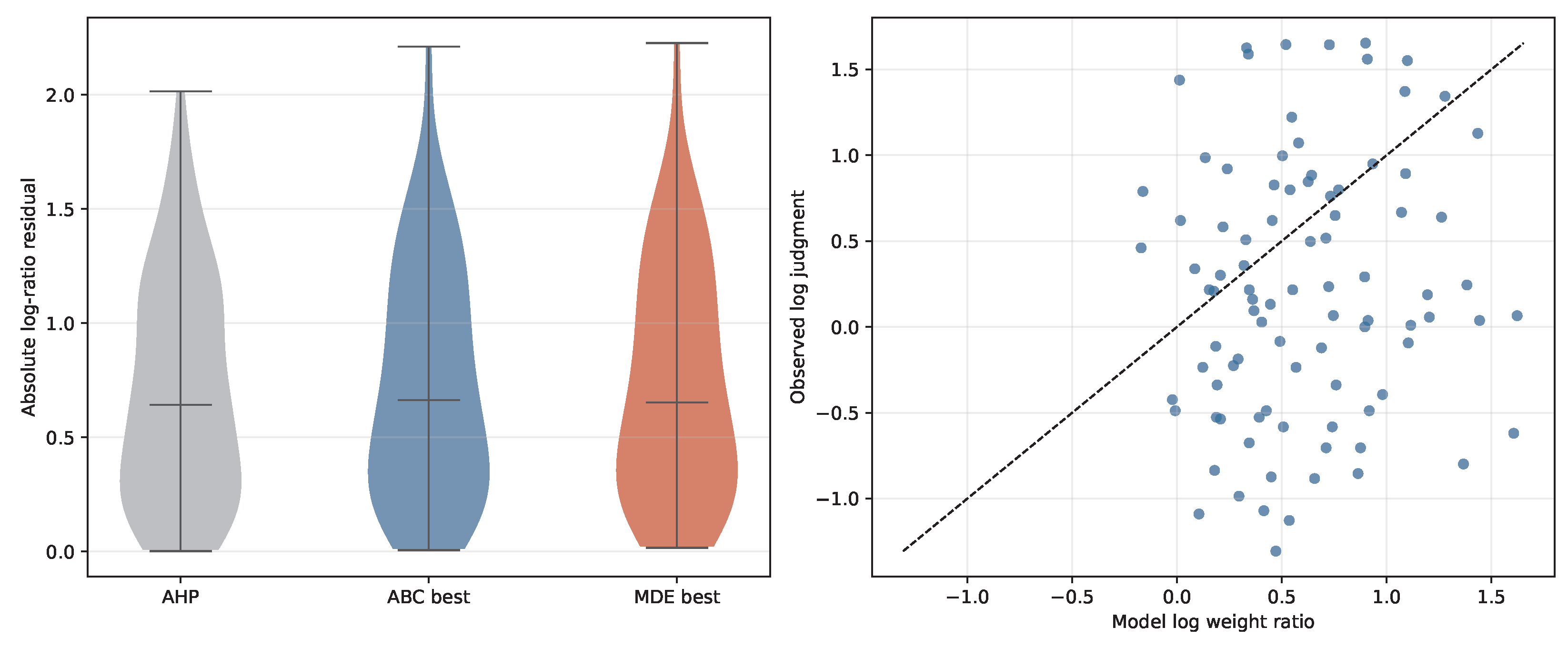
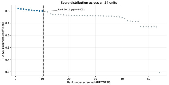
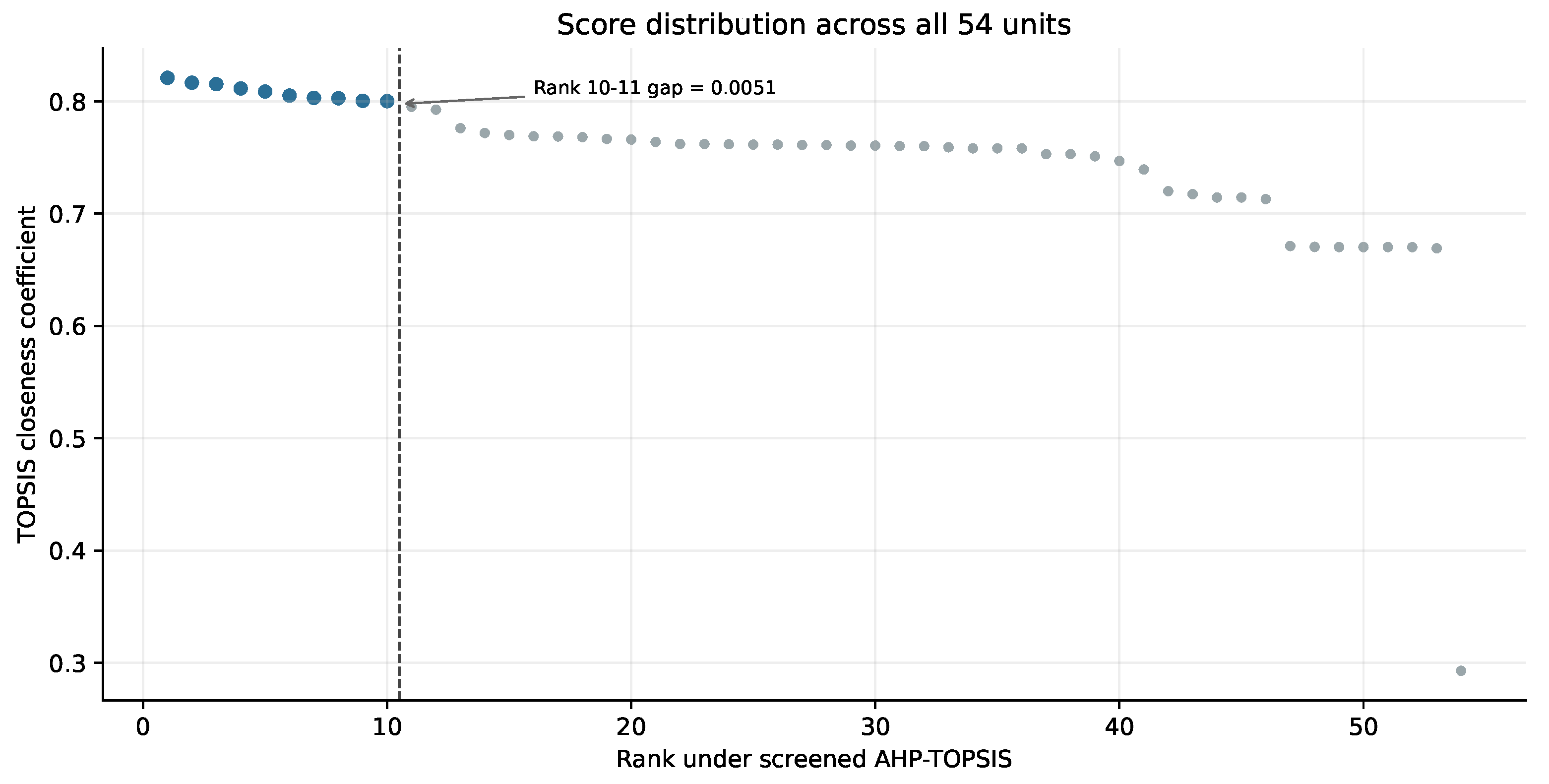
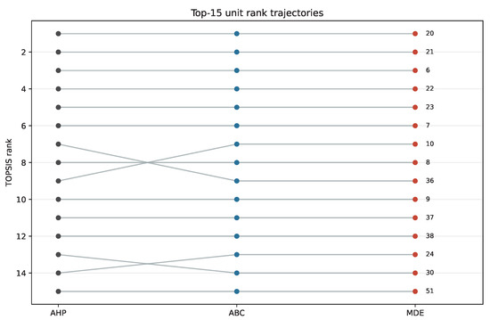
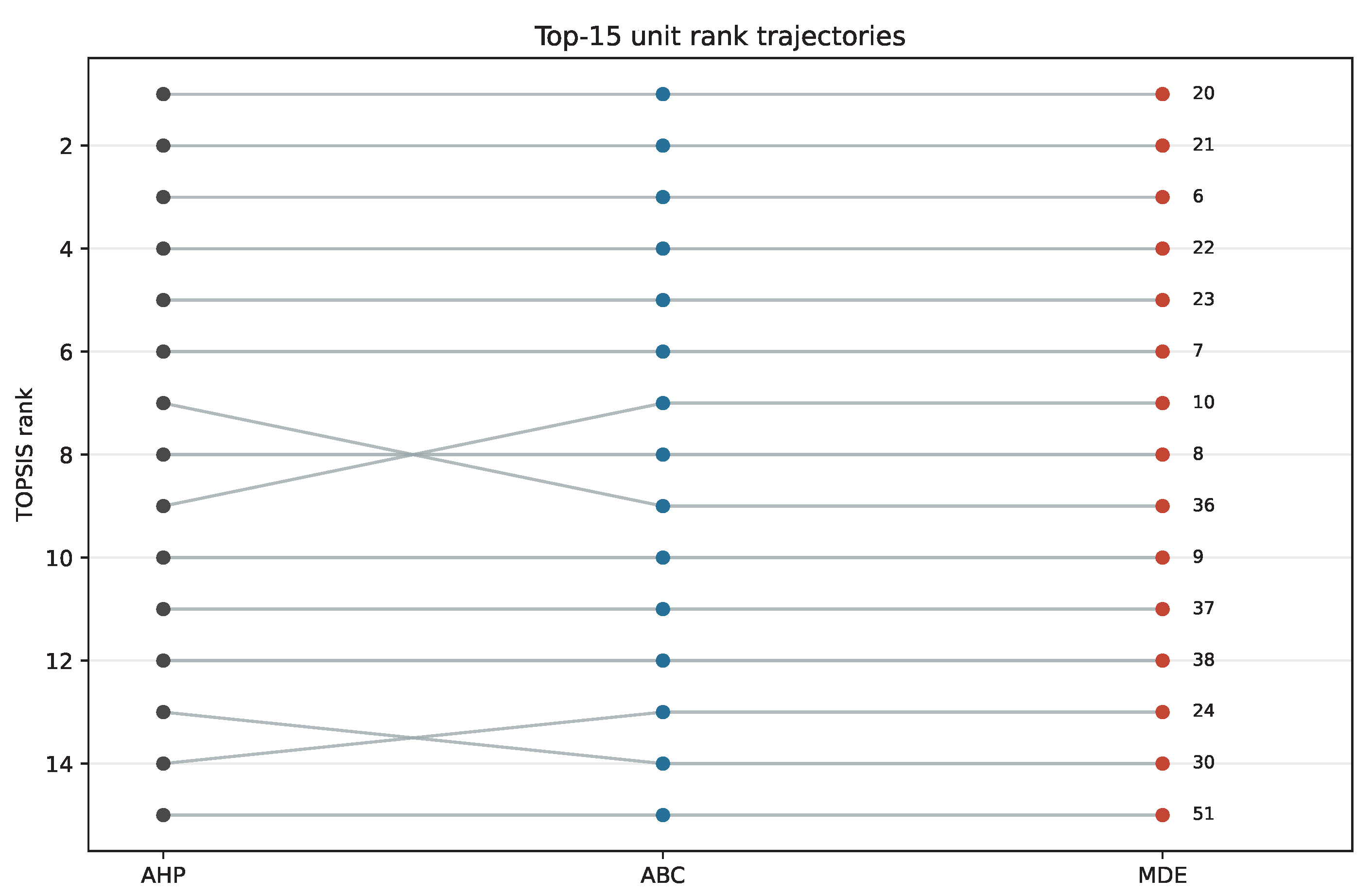
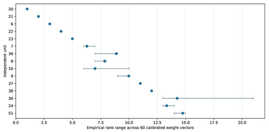
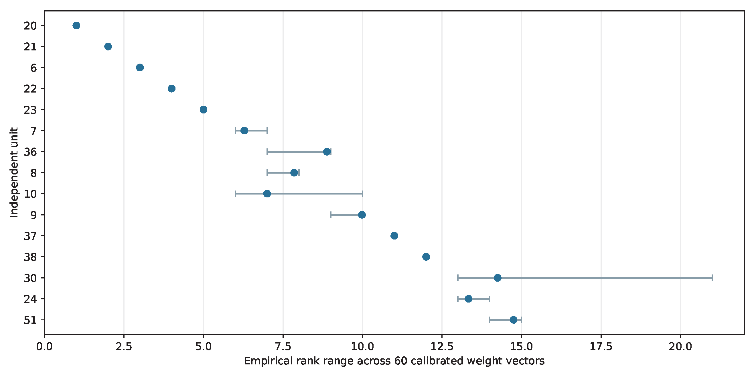
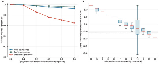
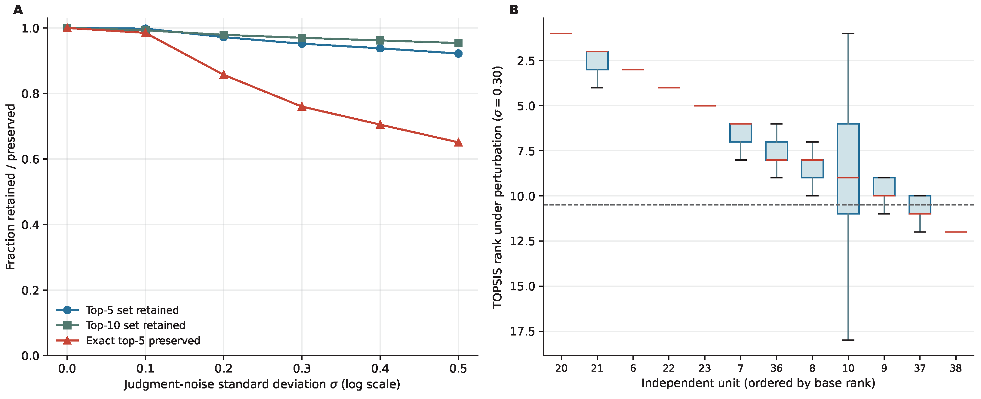
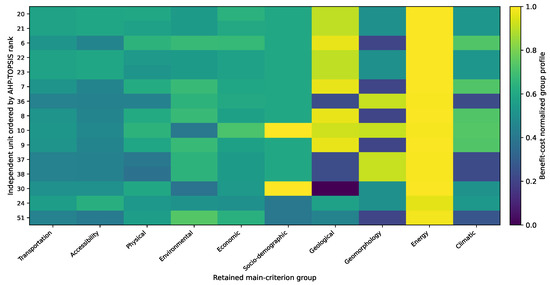
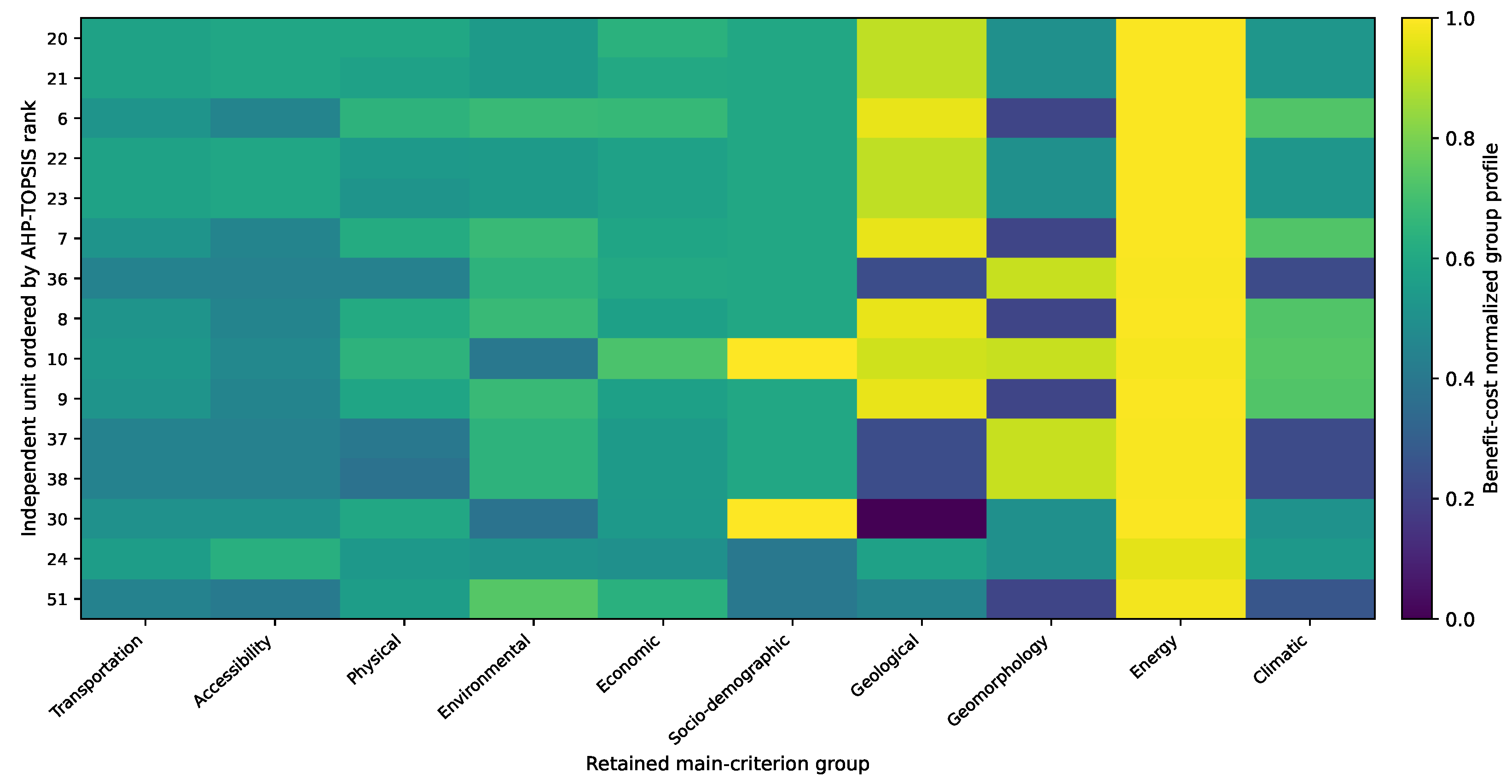
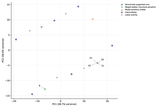
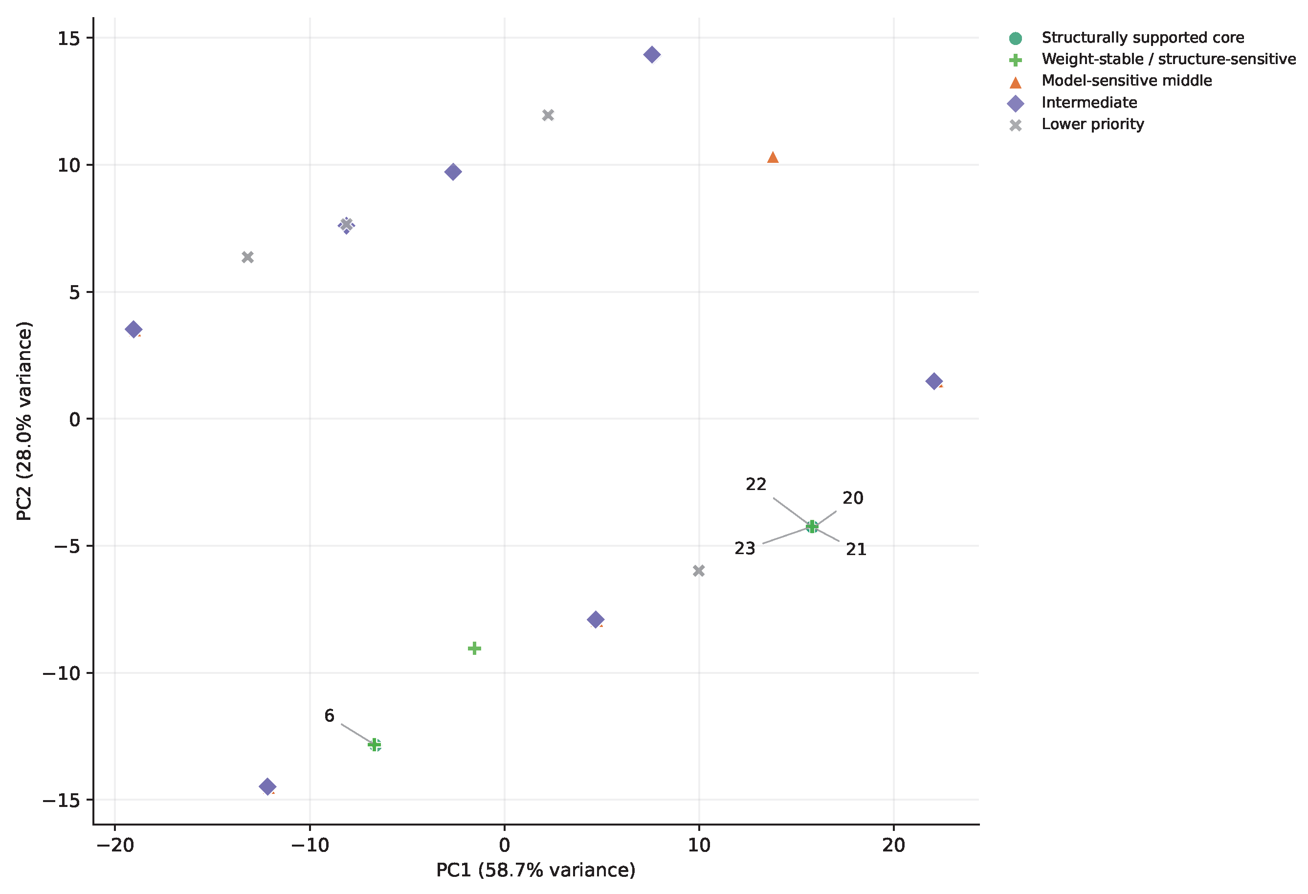
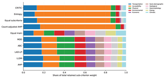
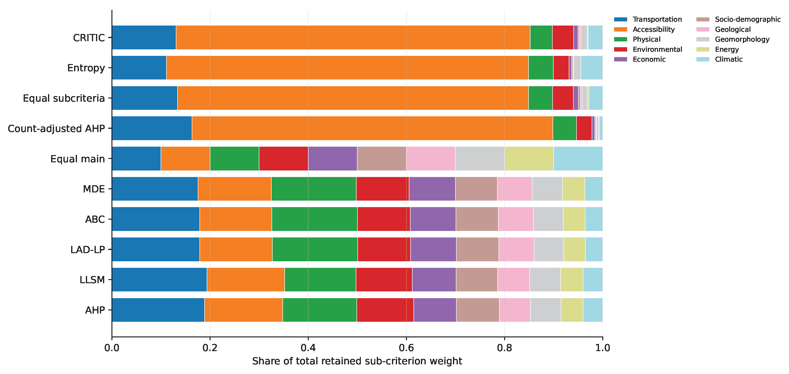
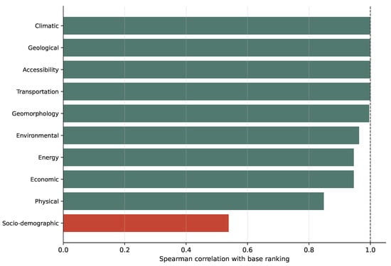
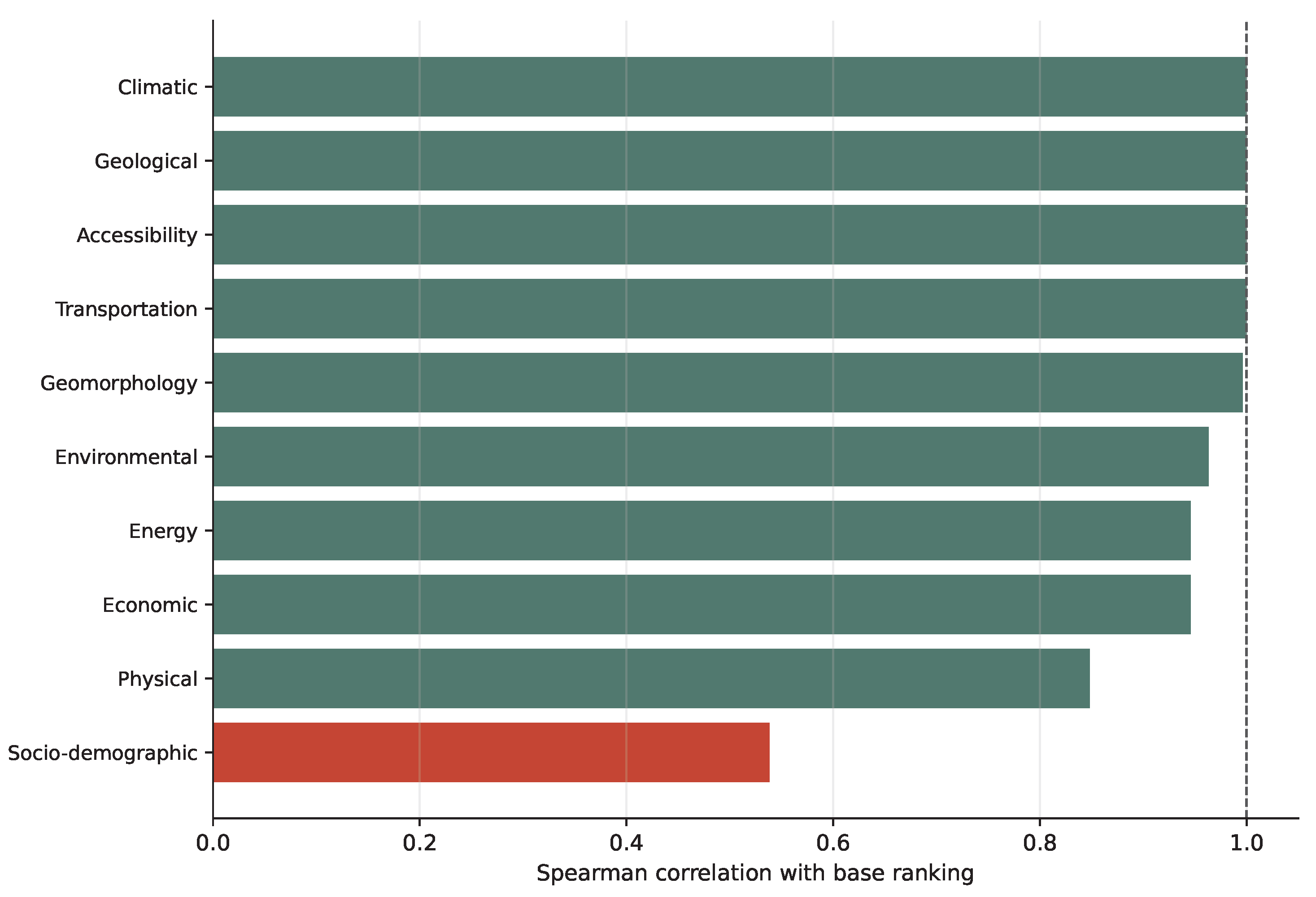
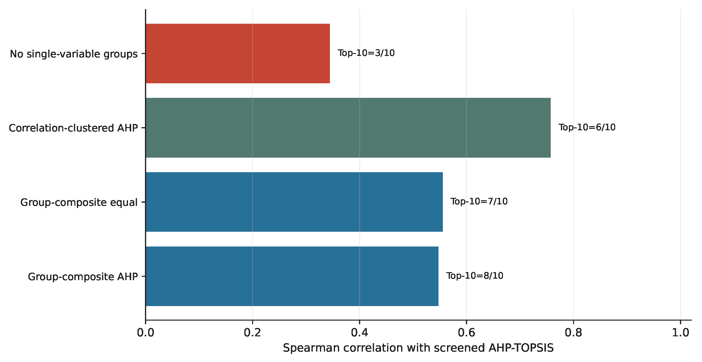

Disclaimer/Publisher’s Note: The statements, opinions and data contained in all publications are solely those of the individual author(s) and contributor(s) and not of MDPI and/or the editor(s). MDPI and/or the editor(s) disclaim responsibility for any injury to people or property resulting from any ideas, methods, instructions or products referred to in the content. |
© 2026 by the authors. Licensee MDPI, Basel, Switzerland. This article is an open access article distributed under the terms and conditions of the Creative Commons Attribution (CC BY) license.