Long-Term Spatiotemporal Dynamics, Trade-Offs, and Future Scenarios of Ecosystem Services in the Urumqi–Changji–Shihezi Urban Agglomeration, Northwest China

Abstract

Ecosystem services (ESs) underpin human well-being and regional development by linking ecological processes with human land–use activities. However, for arid oasis urban agglomerations, evidence remains limited on long-term ES changes, landscape-type contributions, and future responses under alternative development pathways. We quantified five ESs in the UCS from 1990 to 2020 using InVEST and statistical allocation methods and related the resulting service maps to landscape-type contributions and service-pair relationships. The PLUS model generated 2030 land–use pathways, which were used to compare ES responses under BAU, ED, and EP scenarios. The LEAS module identified how climatic, socioeconomic, topographic, and accessibility factors contributed to land–use expansion and thereby indirectly shaped ES patterns. The results show that (1) from 1990 to 2020, food production (FP) increased with fluctuations from 16.30 to 62.06 t·km⁻², whereas water yield (WY), carbon storage (CS), soil conservation (SC), and habitat quality (HQ) declined by 27.8%, 5.7%, 27.0%, and 5.4%, respectively; (2) the five ecosystem services showed clear spatial heterogeneity, with food production characterized by high values in the central oasis plain and low values in the northern and southern parts, whereas the other four services showed a south-high/north-low gradient; forestland, grassland, and water bodies were the major landscape types supporting ecosystem-service supply; (3) ecosystem-service interactions changed dynamically: FP showed clear Pearson trade-offs with HQ and weak trade-offs with SC, whereas WY-CS, WY-SC, CS-SC, SC-HQ, WY-HQ, and CS-HQ were mainly synergistic; FP-WY and FP-CS also showed positive Pearson correlations, indicating that food-production expansion in oasis areas was partly coupled with water-resource and cropland–related carbon-storage patterns; and (4) the 2030 scenario simulations showed differentiated responses: under BAU and ED, FP remained nearly stable or slightly decreased, whereas WY, CS, SC, and HQ increased slightly; under EP, all five services improved relative to 2020, with FP, WY, CS, SC, and HQ increasing by approximately 4.08%, 2.33%, 3.13%, 9.60%, and 0.79%, respectively, making EP the most favorable pathway for enhancing ecosystem-service supply and mitigating FP-related trade-offs. The results identify where provisioning gains conflict with water, soil, carbon, and habitat functions and provide a basis for differentiated oasis management in Urumqi, Changji, Shihezi, and Wujiaqu.

1. Introduction

In arid oasis systems, a central ecological concern is how land–use change reallocates limited water and land resources among food production, urban growth, soil retention, carbon storage, and habitat maintenance [1]. Ecological degradation, water scarcity, biodiversity loss, and climate warming have increasingly weakened ecosystem-service functions. As a result, ecological security and sustainable resource use are especially difficult to maintain in fragile, resource-limited arid regions [2]. Oases concentrate water, soil, atmospheric, and biological resources, forming the ecological foundation for settlement and production in arid regions [3,4]. Ecosystem-service assessment converts changes in land, water, vegetation, and habitat conditions into indicators that can be compared across space and time [5]. This comparison is particularly important in arid oases, where agriculture, urban expansion, and ecological conservation rely on the same limited water-land base.

Ecosystem services provide ecological conditions and environmental benefits that sustain human activities and development [6]. Quantifying ESs helps characterize natural-asset status and ecosystem functions [7]. It also supports ecological protection, restoration, and compensation measures in areas with weak ecological functions [8]. Continued urbanization has intensified conflicts between socioeconomic development and natural ecosystems, making ES assessment, landscape-pattern change, and ecological security key topics in related research [9,10,11]. Existing studies have examined ES classification [12], valuation [13], spatial mapping [14], formation mechanisms and drivers [15], and links with human well-being [16]. Research has also expanded across scales and ecosystem types, including forest [17], watershed [18], and urban ecosystems [19]. Studies related to human well-being increasingly focus on urban forests, urban green spaces, and green infrastructure [20,21]. ES assessment has been applied to different landscape systems, spatial scales, and service types, including wetlands, lakes, watersheds, and cities [22,23,24,25]. Methodologically, research can generally be categorized into three types: traditional market valuation methods, value equivalent factor methods, and computer-based model assessment approaches [26,27]. Remote sensing enables repeated, large-area monitoring of ESs and supports biodiversity conservation and natural-asset assessment [28,29]. However, it must be noted that most current studies focus on ecologically sound, economically developed regions or specific nature reserves while paying insufficient attention to fragile areas such as arid oasis urban agglomerations. For these regions, evidence remains limited on long-term ES changes under combined natural and human influences and on their spatiotemporal evolution. Furthermore, a research blind spot persists regarding the development and evolution of ecosystem services and their trade-off/synergistic relationships under different future development scenarios, which limits the balanced development and protection of natural resources and constrains the healthy, sustainable growth of regional economies and societies. Given the unique physical geographical conditions of arid regions—characterized by fragile ecological environments, poor ecosystem resilience, and low adaptability—ecosystem functions are highly susceptible to damage during socioeconomic development. The paucity of relevant research targeting underdeveloped arid oasis urban agglomerations thus restricts the coordinated development of regional ecosystem health and the socioeconomic system.

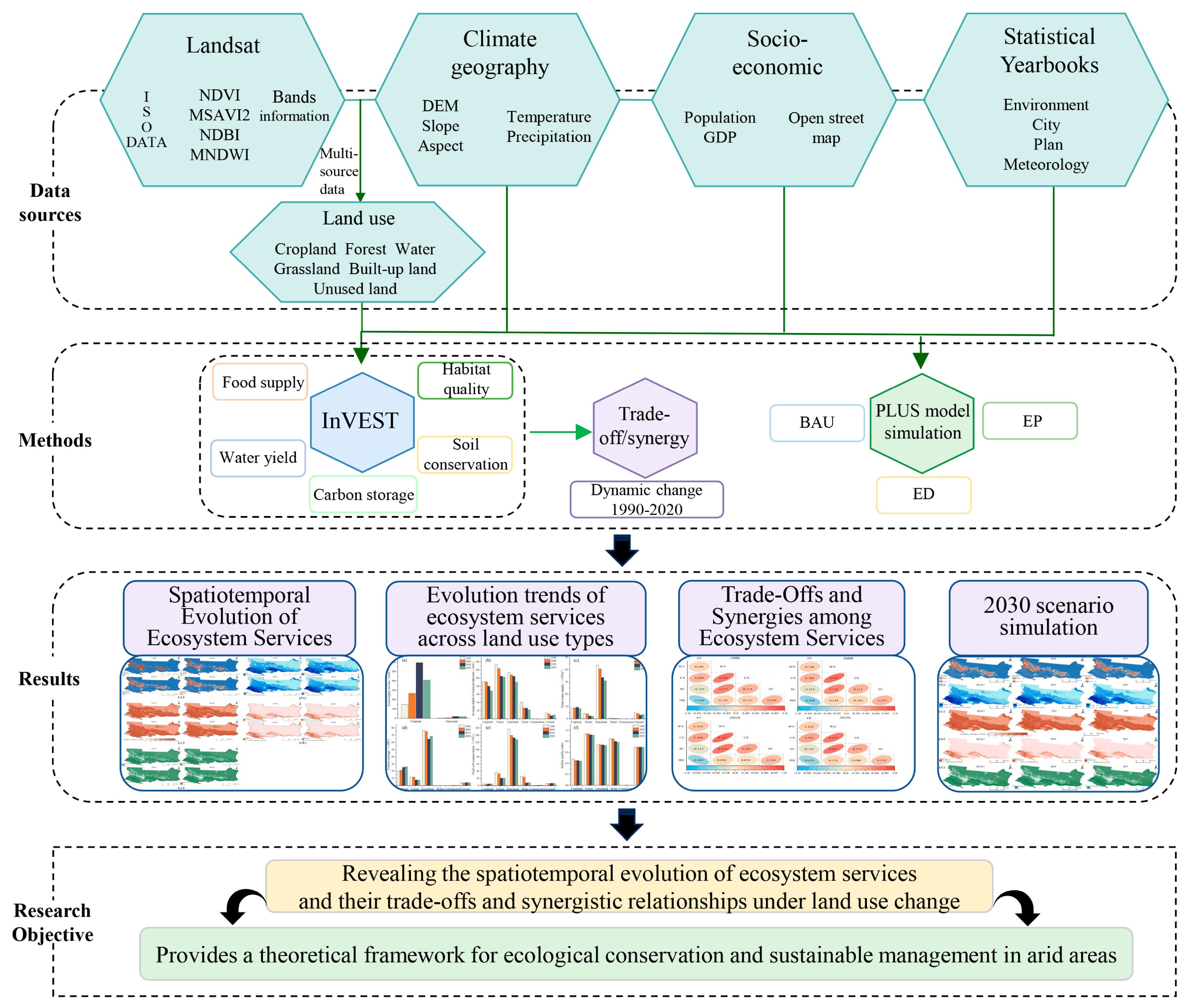
The Urumqi–Changji–Shihezi urban agglomeration (UCS) lies in arid Northwest China. It is the political and economic core of Xinjiang and an important node in the “Belt and Road” Initiative. Under the influence of Reform and Opening-up, the Western Development Strategy, and regional integration policies, the UCS has undergone rapid socioeconomic growth and increasing development intensity. However, its fragile ecological baseline has made oasis landscape degradation and declining ecological functions increasingly prominent, creating constraints on green regional development and resident well-being. Although ES research has advanced in many regions, underdeveloped arid urban agglomerations often combine delayed development with rapid growth pressure. Together with the region’s distinct natural and human influences, this makes the spatiotemporal evolution of ESs in the UCS different from that in more humid or economically mature regions. Accordingly, this study addresses three questions: (1) How do ESs and landscape–type contributions vary across space and time in the UCS? (2) How do trade-off/synergy relationships among ESs evolve? (3) How do climatic, socioeconomic, topographic, and accessibility factors contribute to land–use expansion, and how do ES patterns and relationships respond under alternative future scenarios? For the UCS, we integrated socioeconomic, meteorological, and remote-sensing datasets. The Integrated Valuation of Ecosystem Services and Tradeoffs (InVEST) model was used to assess ES changes from 1990 to 2020. Landscape–type analysis was then used to compare ES supply among land categories, and Pearson correlation was used to identify ES trade-offs and synergies. Finally, the Patch-generating Land Use Simulation (PLUS) model was used to quantify land–use expansion drivers and compare 2030 ES responses under business-as-usual, economic development, and ecological protection scenarios. By linking historical ES assessment with scenario-based comparison, this study provides evidence for ecological restoration, ES enhancement, and sustainable oasis management. Figure 1 illustrates the research framework of this study.

2. Materials and Methods

2.1. Study Area

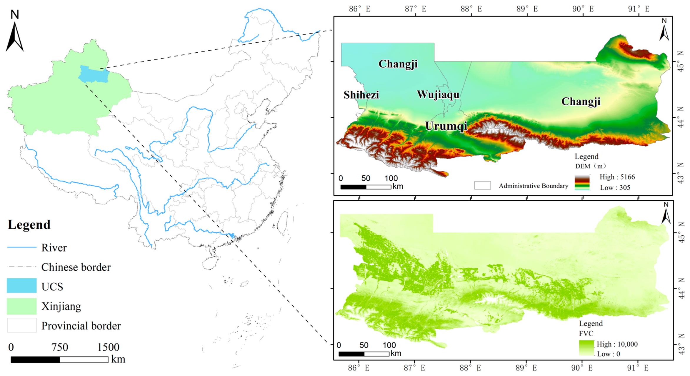
The study area covers Urumqi, Changji Hui Autonomous Prefecture, Shihezi, and Wujiaqu in northern Xinjiang, China (42°52′ N–45°28′ N, 88°40′ E–91°33′ E; Figure 2). It spans the northern Tianshan piedmont, the central oasis belt, and the southern edge of the Junggar Basin, with an area of about 86,000 km². The geomorphology is predominantly characterized by alluvial fan plains, exhibiting a terrain that is generally higher in the south and lower in the north, with elevations spanning from 450 to 2200 m. The region has a temperate continental arid climate, with annual precipitation of only 160–220 mm, evaporation of approximately 2000–2800 mm, and an aridity index above 4.0. Glacier meltwater and groundwater are the main sources of water replenishment and largely determine the stability of oasis agriculture, settlements, and ecological land.

In 2020, the permanent population of the UCS region reached 6.7423 million, accounting for 26.08% of the total population of Xinjiang [30,31]. Long-term monitoring data demonstrate that the population proportion of this region has steadily remained above one-fifth of the entire Xinjiang region and shows a continuous growth trend, rendering it the core zone with the highest population concentration and the most vibrant economic activity in Xinjiang. Concurrently with the accelerated urbanization process, the metropolitan area centered on Urumqi has become increasingly mature. Consequently, the resulting high-intensity anthropogenic activities and land–use shifts are exerting persistent stress and perturbations on the structural integrity and service functions of the regional ecosystem.

2.2. Data Sources

The land–use dataset was derived from Landsat–based interpretation and harmonized with climate, soil, hydrological, NDVI, and statistical datasets for ecosystem-service modeling. Monthly evapotranspiration and precipitation datasets were obtained from the National Earth System Science Data Center. NDVI statistics, soil-property data, and watershed/hydrological vector data were obtained from the Resource and Environment Science and Data Center of the Chinese Academy of Sciences. Statistical data, including the Xinjiang Statistical Yearbook and the Statistical Yearbook of Xinjiang Production and Construction Corps, were collected from CNKI and the Statistics Bureau of Xinjiang Uygur Autonomous Region. The core parameters of the InVEST modules were localized according to the climatic, soil, vegetation, hydrological, and land–use conditions of the UCS region. Specifically, the water-yield module used annual precipitation, reference evapotranspiration, plant available water content, root-restricting layer depth, root depth, the vegetation evapotranspiration coefficient (Kc), and vegetation-cover attributes; the carbon-storage module used the carbon densities of aboveground biomass, belowground biomass, soil organic carbon, and dead organic matter; the SDR module used rainfall erosivity (R), soil erodibility (K), the cover-management factor (C), the support practice factor (P), and SDR routing parameters; and the habitat-quality module used threat weights, maximum influence distances, decay functions, habitat suitability, and sensitivity coefficients. These parameters were compiled from the InVEST user guide, regional studies in arid and semi-arid areas of Xinjiang and Northwest China, soil and climate raster datasets, and the actual model input files used in this study. The complete parameter tables and source files are provided in Supplementary Tables S1–S5. All geospatial data were standardized and preprocessed using the World Geodetic System 1984 (WGS84) and Albers projection, with a unified spatial resolution of 250 m. For the PLUS-LEAS driving-factor analysis, 15 explanatory variables were selected to represent climate, socioeconomic development, topography, soil conditions, water-resource constraints, and accessibility, including precipitation, temperature, GDP, population, elevation, slope, soil type, distance to water bodies, distance to government centers, distance to railways, and distance to different road grades. These driving-factor rasters were resampled and matched to the land–use datasets to support the quantitative identification of land–use expansion mechanisms from 2010 to 2020. The land–use dataset and the baseline PLUS scenario framework employed in this study are derived from prior research on land use and landscape patterns in the UCS region—work that focused on land–use/land–cover change (LUCC) dynamics, landscape-pattern evolution, driving mechanisms, and future land–use simulation [32]. Building upon this foundation, the present study shifts its focus from land–use change itself to ecosystem-service provision, the contributions of different landscape types, trade-off and synergy relationships, and ecosystem-service responses across multiple scenarios as modeled by InVEST.

2.3. Methods

2.3.1. Food-Production Service

Food production provides essential food resources for residents within a region. Considering the land–use structure, agricultural statistics, and animal husbandry characteristics of the UCS, this study used a locally calibrated NDVI-based allocation model to quantify food production. The model was not based on a fixed universal empirical coefficient; instead, annual production totals from local statistical yearbooks were used as control totals, and NDVI was used as the spatial allocation weight within the corresponding land–use masks. Specifically, grain, vegetable, and fruit production were assigned to cropland, while meat, milk, and egg production were assigned to grassland. These categories represent the dominant terrestrial agricultural and pastoral products in the UCS and are consistent with the oasis agriculture and grassland husbandry systems of Xinjiang. The model is expressed as follows [33,34]:

$${FG}_i={\displaystyle \frac{{NDVI}_i}{{NDVI}_{sum}}}\times {FG}_{sum}$$

(1)

In the equation, ${FG}_i$ denotes the allocated yield of grain, vegetables, meat, eggs, and dairy products for spatial unit $i$ (t·km⁻²); ${FG}_{sum}$ represents the total regional yield of grain, vegetables, meat, eggs, and dairy products (t); ${NDVI}_i$ is the Normalized Difference Vegetation Index (NDVI) raster value of unit $i$; and ${NDVI}_{sum}$ is the cumulative NDVI value across the regional cropland or grassland areas. The data are derived from local statistical records for Urumqi, Changji Hui Autonomous Prefecture, and Shihezi; consequently, the sum of pixel-level yield values for each year is constrained by the total observed yield of the region.

2.3.2. Water-Yield Service

Water yield is a fundamental regulating service that maintains ecological balance and supports human survival, and it is especially important in arid regions. The water-yield module of the InVEST model applies the water-balance principle to estimate water yield [35]:

$${WY}_i=\left(1-{\displaystyle \frac{{AET}_i}{P_i}}\right)\times P_i$$

(2)

where ${WY}_i$ represents the water yield of the $i$-th pixel (mm), ${AET}_i$ (mm·y⁻¹) denotes the annual actual evapotranspiration on the $i$-th pixel derived from the land–use raster data, and $P_i$ (mm·y⁻¹) represents the annual precipitation on the $i$-th pixel. The water-yield parameters were prepared from the actual InVEST input files and localized using regional climatic, soil, and land–use data (Supplementary Table S1). Annual precipitation and reference evapotranspiration were prepared as year-specific raster inputs, while plant available water content and root-restricting layer depth were derived from soil-property datasets. The biophysical table assigned root depth, Kc, and vegetation-cover attributes to each land–use class. Root depth was set to 1550 mm for cropland, 6000 mm for forestland, 1700 mm for grassland, and 1 mm for water bodies, built-up land, and unused land. The Kc values were 0.75, 1.00, 0.80, 1.10, 0.30, and 0.50 for cropland, forestland, grassland, water bodies, built-up land, and unused land, respectively. The seasonality constant Z was calibrated according to arid-zone water-yield characteristics and set to 0.02, 0.02, 0.025, and 0.03 for 1990, 2000, 2010, and 2020, respectively.

2.3.3. Carbon-Storage Service

The carbon-storage module of the InVEST model calculates carbon storage mainly from the carbon densities of different land–cover types, including soil carbon, dead organic matter, aboveground biomass, and belowground biomass. Using the land–use/land–cover grid as the assessment unit, carbon storage is obtained by multiplying the mean carbon-pool density of each landscape type by its corresponding area. The calculation is as follows [36]:

$$C_k=C_{above}+C_{below}+C_{soil}+C_{dead}$$

(3)

$$C_{total}={\displaystyle \sum _{k=1}^n}{A}_k\times C_k\left(k=1, 2,\dots ,n\right)$$

(4)

where $C_k$ represents the carbon stock of the raster unit for the $k$-th land–use type, $C_{above}$ denotes the aboveground vegetation carbon stock, $C_{below}$ the belowground vegetation carbon stock, $C_{soil}$ the soil carbon stock, and $C_{dead}$ the dead organic matter carbon stock. $C_{total}$ represents the total carbon stock in the UCS region, $A_k$ denotes the total area of each land–cover type, and $n$ is the total number of land-use types. The carbon-density parameters were assigned according to the four carbon pools required by the InVEST carbon-storage module: aboveground biomass carbon, belowground biomass carbon, soil organic carbon, and dead organic matter carbon (Supplementary Tables S2). The values were compiled from the InVEST parameter framework and regional studies and were adjusted to the six land–use classes used in this study. Forestland was assigned the highest total carbon density because of its high aboveground, belowground, and soil carbon pools, followed by grassland and cropland. Water bodies, built-up land, and unused land were assigned lower carbon densities because of their limited vegetation cover and soil organic matter storage.

2.3.4. Soil-Conservation Service

Soil conservation is an important regulating service for regional ecological security. This study used the sediment delivery ratio (SDR) module of the InVEST model to calculate potential and actual soil loss. The total soil-conservation amount was defined as the difference between potential and actual soil loss [37]:

$${SD}_i=\left(R_i\times K_i\times {LS}_i\right)-\left(R_i\times K_i\times {LS}_i\times C_i\times P_i\right)$$

(5)

In the equation, $R_i$, $K_i$, ${LS}_i$, $C_i$ and $P_i$ represent the rainfall erosivity factor, soil erodibility factor, slope length and steepness factor, cover-management factor, and support practice (soil and water conservation) factor, respectively. ${SD}_i$ denotes the soil conservation amount (soil retention) of the $i$-th land–use raster unit. The SDR module parameters were prepared from raster inputs and land–use-specific biophysical coefficients (Supplementary Table S3). Rainfall erosivity (R) was generated from annual precipitation data for each study year, and soil erodibility (K) was derived from soil-property data. The mean R values were 357.03, 342.43, 288.47, and 275.55 for 1990, 2000, 2010, and 2020, respectively, while the K factor ranged from 0.0084 to 0.0205 with a mean of 0.0153. The cover-management factor (C) and support practice factor (P) were assigned by land–use class. For example, C/P values were 0.18/0.40 for cropland, 0.03/1.00 for forestland, 0.15/1.00 for grassland, 0/0 for water bodies and built-up land, and 1.00/1.00 for unused land. The global SDR parameters recorded in the model run files were k = 2, IC0 = 0.5, SDRmax = 0.8, lmax = 122, and threshold flow accumulation = 1000.

2.3.5. Habitat-Quality Service

The habitat-quality module of the InVEST model was used to calculate the regional habitat quality index (HQ). In this study, HQ is not defined as an additive combination of habitat suitability, biodiversity, ecological-resource richness, and social or political acceptance; instead, it is a dimensionless, model-based proxy for relative habitat condition, calculated from land–use-based habitat suitability and cumulative degradation pressure from threat factors. The index ranges from 0 to 1; higher HQ values indicate higher modeled habitat suitability, lower degradation pressure, and stronger potential biodiversity-support capacity under the given land–use and disturbance conditions. The formula is as follows [38]:

$$Q_{xj}=H_j\left[1-\left({\displaystyle \frac{D_{xj}^z}{D_{xj}^z+k^z}}\right)\right]$$

(6)

where $Q_{xj}$ represents the habitat quality index of raster cell $x$ for land–use type $j$, $H_j$ denotes the habitat suitability of land–use type $j$, $D_{xj}$ indicates the habitat degradation degree of raster cell $x$ for land–use type $j$, and $z$ and $k$ are constants, where $z$ is the model’s default normalization parameter and $k$ is the half-saturation coefficient. The half-saturation constant $k$ determines how strongly habitat degradation is translated into habitat-quality reduction. $k$ controls the curvature and sensitivity of HQ to degradation; a smaller $k$ makes HQ more sensitive to low levels of degradation, whereas a larger $k$ smooths the degradation response. The habitat-quality parameters were localized by combining the regional land–use pattern, human-disturbance sources, and the InVEST habitat-quality parameterization framework (Supplementary Tables S4 and S5). Six threat factors were considered: cropland, built-up land, unused land, village settlements, roads, and railways. For each assessment year, threat rasters were prepared from the corresponding land–use and infrastructure datasets, and the maximum influence distance, weight, and decay function were specified in the threat table. Built-up land had the highest threat weight, reflecting strong disturbance from urban construction, while village settlements, roads, railways, cropland, and unused land represented additional anthropogenic or land–use disturbance sources. Habitat suitability and sensitivity to each threat were assigned for each land–use class. Forestland and water bodies had high habitat suitability, whereas built-up land was assigned a habitat suitability of 0 because of its intensive anthropogenic disturbance. The half-saturation constant was set to 0.05. Therefore, the additivity in the habitat-quality module applies only to the standardized degradation effects of different threat factors, not to heterogeneous ecological or social concepts. Threat factors are made comparable through dimensionless weights, distance-decay functions, maximum influence distances, and land–use-specific sensitivity coefficients. The final HQ value is obtained by combining habitat suitability with the cumulative degradation index through the InVEST nonlinear response function. Thus, HQ should be interpreted as a relative spatial index of modeled habitat condition rather than a direct field measurement of biodiversity, species abundance, ecological-resource richness, or social acceptance.

2.3.6. Identification of Ecosystem-Service Trade-Offs and Synergies

Correlation analysis was used to identify the direction and relative strength of relationships among ecosystem services [39,40,41]. Pearson correlation coefficients were used as the main indicator because they measure linear covariation in the original magnitudes of ecosystem-service values and are therefore suitable for evaluating whether increases in one service are accompanied by increases or decreases in another service at the regional scale. However, because raster-based ecosystem-service variables may be non-normally distributed and affected by zero values and spatial heterogeneity, Spearman’s rank correlation and Kendall’s tau were also calculated as robustness checks. Spearman and Kendall correlations measure rank-based monotonic associations and are less sensitive to the original units and extreme values. It should be noted that the Pearson correlation coefficients were used to identify regional-scale trade-off/synergy directions and temporal changes rather than local spatial clustering patterns. The correlation analysis was conducted using grid-based samples. A 1500 m fishnet was generated over the UCS region, and the centroid of each grid cell was used as the sampling unit. The values of food production, water yield, carbon storage, soil conservation, and habitat quality were extracted from the corresponding raster layers to the grid centroids under the same projection and spatial extent. Grid cells containing NoData values in any ecosystem-service layer were excluded, while zero values were retained because they represent meaningful low or absent ecosystem- service supply rather than missing data.

2.3.7. PLUS Model, Driving-Factor Analysis, and Multi-Scenario Simulation

The PLUS model is an integrated model that simulates spatial and temporal land–use/land–cover (LULC) change at the patch scale using raster data. Developed by Liang et al. [42], it is an improved version of cellular automata (CA) models and consists mainly of the land–use expansion strategy analysis (LEAS) module and the cellular automata based on multiple random seeds (CARS) module. The model performs well in mining land–use change drivers and simulating patch-level land–use transitions, effectively addressing the limitations of traditional CA models, particularly their insufficient attention to natural land–use change and patch-generation processes. The PLUS simulation was implemented in two steps. First, the land expansion analysis strategy (LEAS) module was used to extract land–use expansion from 2010 to 2020 and to estimate the development probability of each land–use type based on natural, socioeconomic, accessibility, and neighborhood factors. Second, the cellular automata based on multiple random seeds (CARS) module was used to simulate the 2020 land–use pattern for model validation and then predict the 2030 land–use pattern under different scenarios. The observed 2020 land–use map was used as the reference map for model validation. To address the quantitative interpretation of driving mechanisms, the LEAS module was used to identify the contribution of driving factors to land–use expansion from 2010 to 2020. Specifically, land–use expansion patches for each target land–use type were extracted by comparing the 2010 and 2020 land–use maps, and random-forest learning was then applied to quantify the relationship between land–use expansion and 15 explanatory variables. The variables included GDP, population, precipitation, temperature, elevation, slope, soil type, distance to water bodies, distance to government centers, distance to railways, and distance to highways, trunk roads, primary roads, secondary roads, and tertiary roads. The contribution of each driving factor was calculated from the increase in model error after introducing random noise into that factor and was normalized as the relative contribution rate. This procedure allowed the climate, socioeconomic, topographic, soil, water-resource, and accessibility effects embedded in the PLUS framework to be quantitatively compared.

Business as usual (BAU) was used as the reference pathway and retained the 2010–2020 transition tendency without additional ecological or economic intervention. In the present study, this scenario serves not as a new land–use modeling contribution but as the baseline for comparing the ecosystem-service consequences of alternative land–use pathways.

Economic development (ED) was designed to test how stronger construction-land demand would influence ES supply through land–use conversion, especially around oasis cities, transport corridors, and desert–oasis fringe areas. On the basis of the 2010–2020 historical transition matrix, the probabilities of cropland, forestland, and grassland being converted to built-up land were increased by 20%, reflecting increased construction-land demand around oasis cities and transportation corridors. The probability of unused land being converted to built-up land was increased by 30%, representing the stronger possibility of development in low-ecological-resistance desert–oasis fringe areas. Meanwhile, the probabilities of built-up land being converted to forestland, grassland, water bodies, and unused land were reduced by 30%, reflecting the path dependence and relative irreversibility of urban construction land under an economic-development pathway. After adjustment, each transition-probability row was normalized to ensure that the total probability remained equal to 1.

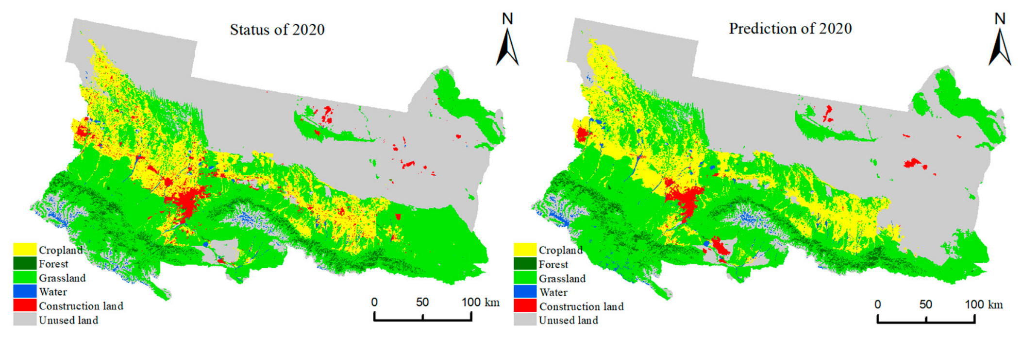
Ecological protection (EP) was designed to test whether stricter protection of cropland, forestland, grassland, and water-source areas could improve regulating and supporting services while maintaining the regional food-production base. Its constraints were linked to territorial spatial planning, ecological conservation redlines, permanent basic farmland protection, water-source conservation, and the arid-region principle of determining urban scale and land development intensity according to water availability. On the basis of the 2010–2020 historical transition matrix, the probabilities of cropland, forestland, and grassland being converted to built-up land and unused land were reduced by 20%, reflecting stricter protection of agricultural and ecological land. The probability of unused land being converted to cropland, forestland, and grassland was increased by 30%, representing ecological restoration and land consolidation in suitable areas. The probabilities of built-up land being converted to forestland and grassland were increased by 10%, representing urban ecological restoration and green-space renewal. The PLUS model was used to simulate the spatial distribution of land use in the UCS in 2020, and the simulation was validated against the observed 2020 land–use distribution (Figure 3). The simulated 2020 land–use map was compared with the observed 2020 map to evaluate whether the land–use pathway generator was reliable enough for ES scenario assessment. The Kappa, OA, and FoM were 0.8352, 0.8922, and 0.8470, respectively, indicating acceptable agreement for subsequent InVEST-based scenario comparison. To avoid reliance on a single accuracy metric, the validation process employed a combination of the Kappa coefficient, Overall Accuracy (OA), and the Figure of Merit (FoM). Based on a comparison between the final 2020 simulation results and the observed data, the metrics were as follows: Kappa coefficient = 0.8352, OA = 0.8922, and FoM = 0.8470. ROC/AUC was not used as a primary validation metric in this study because the final output of the CARS model is a multi-category land–use map rather than a binary probability surface. This scenario design links land–use change constraints with regional ecological-protection policies and helps evaluate the potential of an ecology-priority pathway to improve ecosystem-service supply in the urban agglomeration.

3. Results

3.1. Spatiotemporal Evolution of Ecosystem Services

3.1.1. Food-Production Service

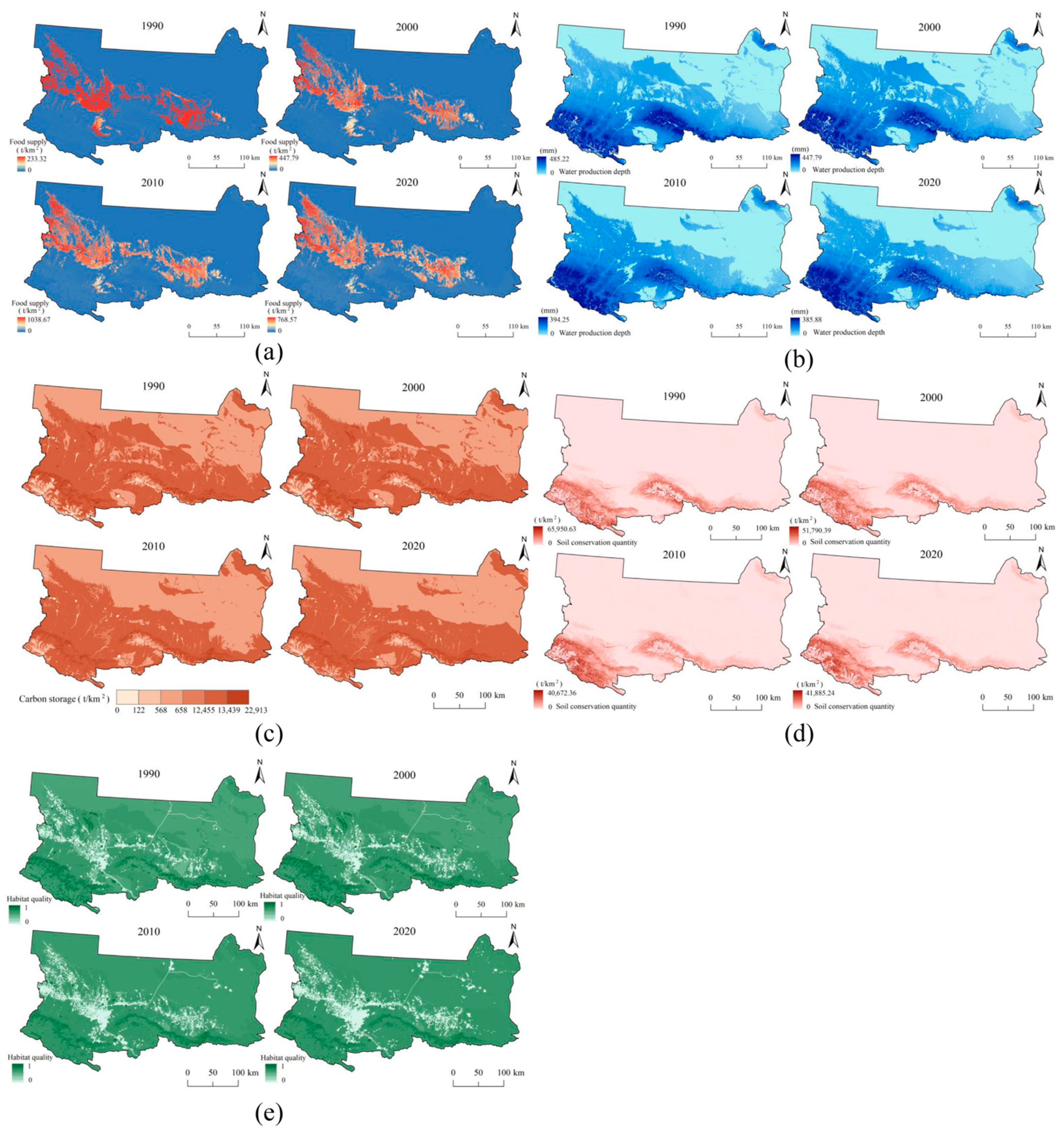
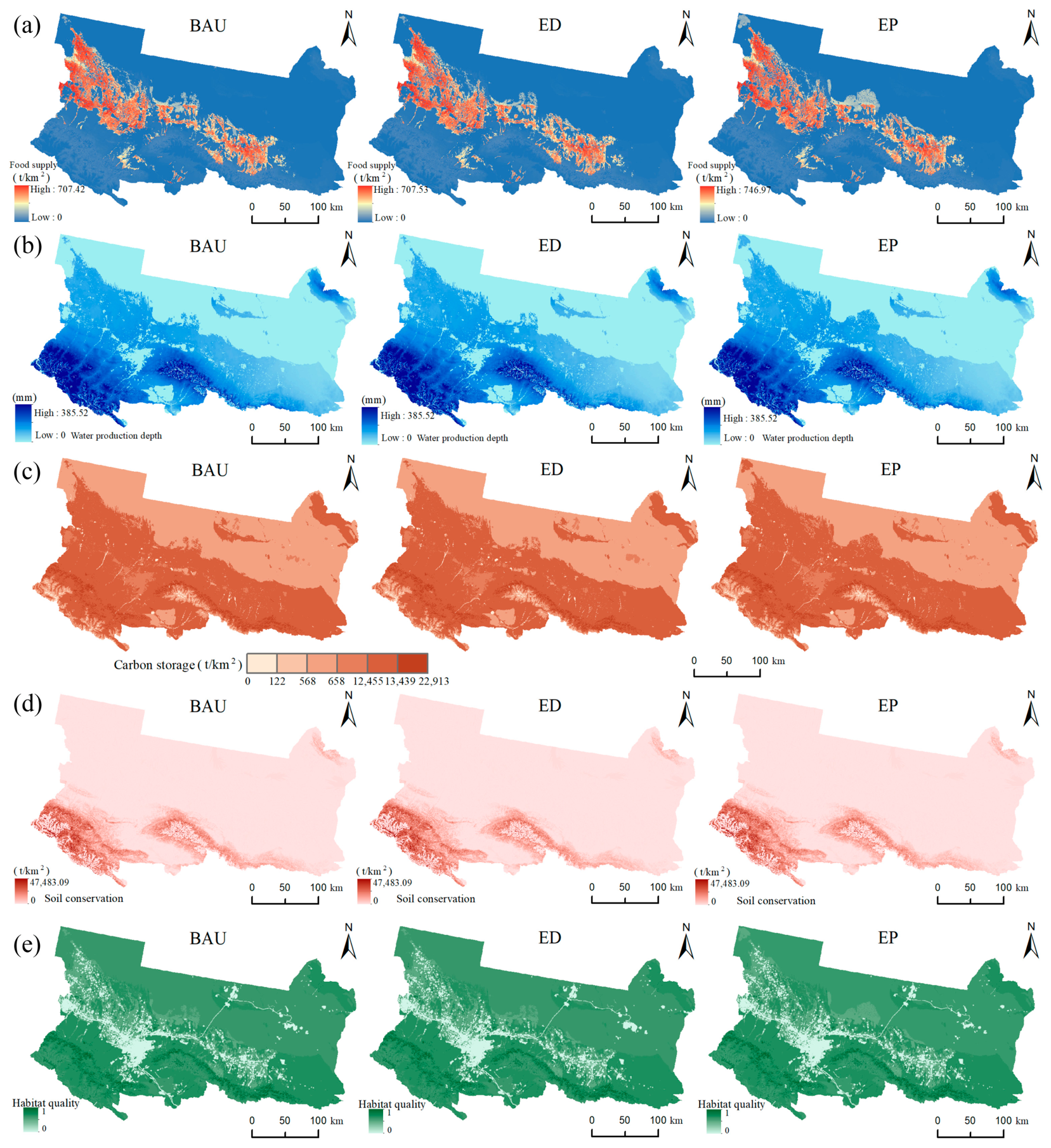
From 1990 to 2020, total food production in the UCS increased overall by approximately 280%, with mean food production values of 16.30, 31.77, 86.05, and 62.06 t·km⁻² in 1990, 2000, 2010, and 2020, respectively. This indicates a staged pattern of rapid increase followed by decline. Spatially, food-supply capacity was higher in the southern and central oasis plains and lower in the northern Gurbantunggut Desert and the high-elevation mountainous areas in the north and south (Figure 4a). The expansion of food production was mainly driven by changes in cropland and grassland use intensity associated with urban–rural development. The increase in food production reflects intensified use of agricultural production resources, especially cropland, but a resource-use mode focused only on provisioning services may intensify competition and trade-offs with ecological resources such as habitat quality.

3.1.2. Water-Yield Service

The total water-yield/mean water-yield depth in the study area was 61.65 × 10⁸ m³/70.10 mm, 57.57 × 10⁸ m³/64.45 mm, 47.98 × 10⁸ m³/54.57 mm, and 44.53 × 10⁸ m³/50.66 mm in 1990, 2000, 2010, and 2020, respectively. The mean water-yield depth decreased from 70.10 to 50.66 mm, a decline of 19.44 mm, indicating continuous degradation. The overall level of water-yield service was low, and the spatial pattern consistently showed a strong south-high/north-low gradient (Figure 4b). Areas with substantial changes were mainly located in the southern high-elevation mountains covered by snow and glaciers and in downstream central areas where water convergence and vegetation cover decreased. Affected by arid climate and high evaporation, northern and eastern areas maintained low water-yield levels. The decline was particularly pronounced from 1990 to 2010 and then slowed. This persistent decrease indicates that the ecological foundation for water-resource regeneration has weakened and that the ecological security of water supply faces severe challenges under the dual stress of a warming–drying climate and intensive development.

3.1.3. Carbon-Storage Service

From 1990 to 2020, total carbon storage in the UCS first decreased and then increased slightly, with values of 11.21 × 10⁹ t, 11.15 × 10⁹ t, 10.16 × 10⁹ t, and 10.57 × 10⁹ t. The average carbon storage per unit area was 7917.54, 7876.40, 7175.56, and 7467.93 t·km⁻², respectively. The spatial pattern of carbon storage remained generally stable and showed a clear south-high/north-low gradient (Figure 4c). Extremely high values were mainly distributed in high-elevation forestland in the southern mountains. High values were widely distributed in southern high-elevation grassland, central cropland, and northern low-elevation grassland, whereas low values were mainly found in urban built-up areas, water bodies, and unused land.

3.1.4. Soil-Conservation Service

The actual total soil conservation in the study area was 14.66 × 10¹⁰ t, 13.11 × 10¹⁰ t, 11.04 × 10¹⁰ t, and 10.70 × 10¹⁰ t in 1990, 2000, 2010, and 2020, respectively, showing an overall decreasing trend. Spatially, the distribution of soil conservation has remained stable over the past 30 years and showed clear elevation zonation. High soil-conservation values were concentrated in high-elevation areas, whereas low values were mainly distributed in low-elevation areas (Figure 4d). Areas with significant changes were mainly located in the southern mountainous high-elevation zones with abundant water-yield capacity and in areas with frequent human activities. Soil conservation was also influenced by the combined effects of precipitation, topography, vegetation cover, and soil conditions.

3.1.5. Habitat-Quality Service

The habitat-quality indices of the UCS in 1990, 2000, 2010, and 2020 were 0.6955, 0.6894, 0.6714, and 0.6583, respectively, showing a fluctuating downward trend. Over the past 30 years, the index has decreased cumulatively by 0.0373, or 5.36%. The decline was most pronounced from 2000 to 2010 (0.0181), indicating accelerated habitat degradation during this period. In terms of spatial pattern and change, habitat quality remained highly stable and changed only slightly. It showed a clear decreasing gradient from south to north, with high values in the southern mountains and low values in the northern desert–oasis ecotone. This pattern is closely related to the region’s natural background and reflects strong altitudinal zonation (Figure 4e).

3.2. Evolution Trends of Ecosystem Services Across Land–Use Types

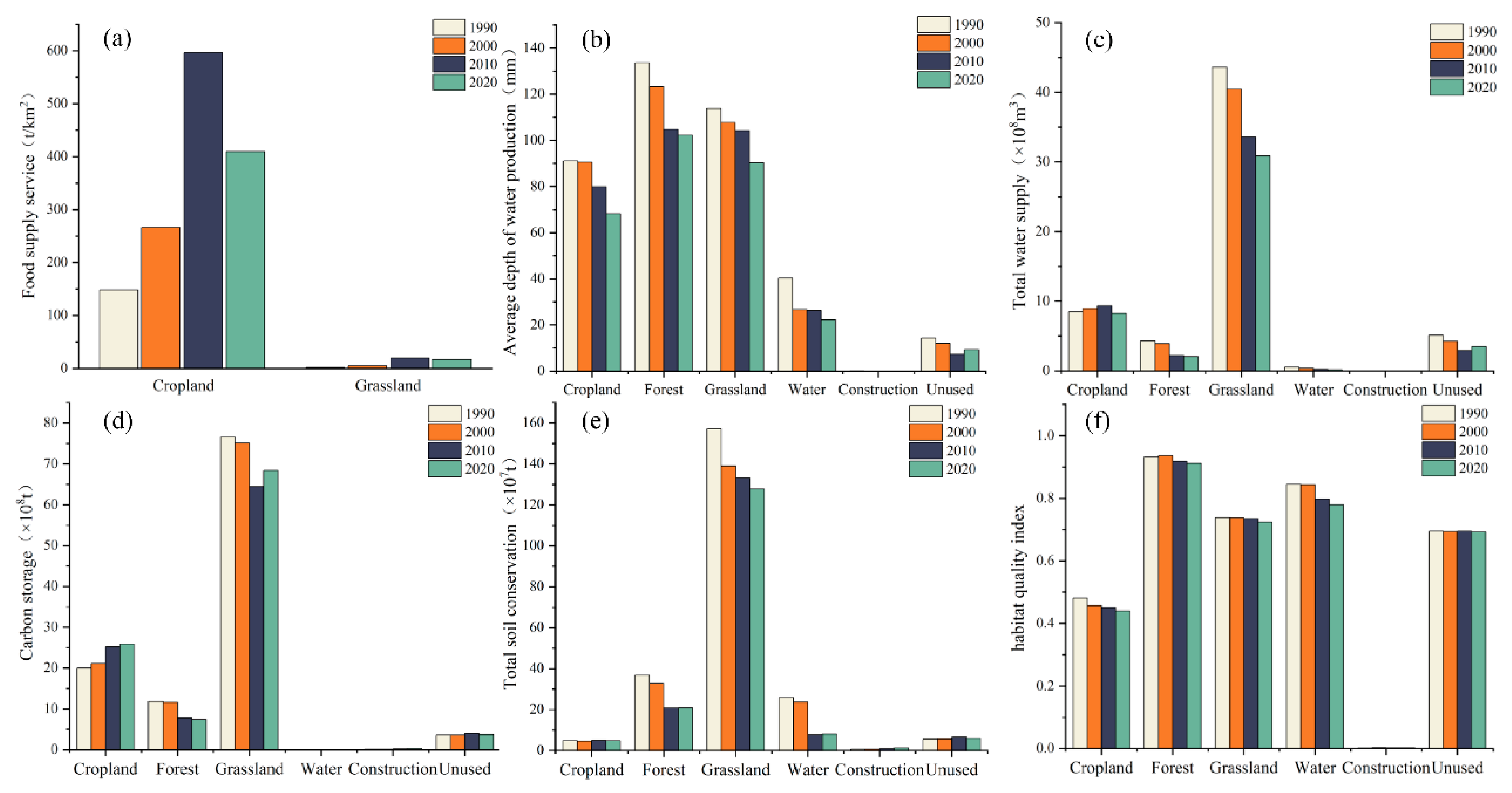
As shown in Figure 5a, food production was assigned only to cropland and grassland according to the locally calibrated NDVI allocation model. Cropland contributed the dominant share of terrestrial food production because grain, vegetable, and fruit outputs were allocated to cropland. Grassland supplied a smaller amount of food production, but its contribution increased from 4.41% in 1990 to 10.19% in 2020, reflecting the rising role of livestock products in the regional food-production structure.

From 1990 to 2020, the mean annual water-yield depth of all land–use types decreased. Forestland, grassland, and cropland had relatively high water-yield capacity, whereas built-up land had the lowest capacity. Water-yield capacity differed markedly among land–use types. In terms of total water-yield capacity by landscape type, grassland contributed the most, followed by cropland, forestland, unused land, water bodies, and built-up land.

From 1990 to 2020, the total carbon-storage service provided by some land–use types fluctuated substantially. Water bodies, built-up land, and unused land contributed relatively little to carbon storage, and no obvious changes were observed for these types. Carbon storage provided by cropland increased, whereas that provided by forestland decreased. Grassland carbon storage first decreased and then increased. Among all land–use types, grassland contributed the largest share of total carbon storage, accounting for more than 60% in each period, followed by cropland and forestland.

The total soil-conservation service provided by grassland, forestland, water bodies, unused land, cropland, and built-up land decreased in that order. During the study period, the total soil-conservation service provided by grassland continued to decrease, whereas forestland and water bodies declined initially and then increased slightly after 2010. Cropland showed a pattern of decrease, increase, and then decrease, with relatively small fluctuations. Unused land first increased and then decreased, while built-up land increased slightly and continuously. Because built-up land occupied a very small area, its contribution to total soil conservation remained negligible.

Habitat quality differed among forestland, water bodies, grassland, unused land, cropland, and built-up land, with mean values of 0.9245, 0.8165, 0.7331, 0.6938, 0.4570, and 0.0022, respectively. The habitat-quality indices of cropland, forestland, grassland, and water bodies generally declined. Forestland first increased and then decreased, whereas cropland, grassland, and water bodies decreased continuously. Overall, compared with other ecosystem services, the habitat-quality service among different land–use types has changed only slightly over the past 30 years and showed a weak overall decline.

3.3. Trade-Offs and Synergies Among Ecosystem Services

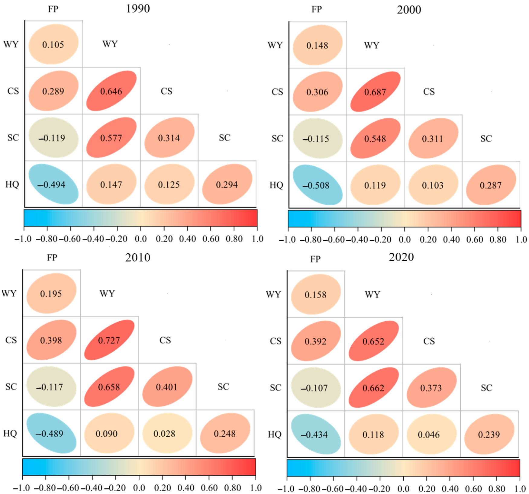
The correlation results represent the overall trade-off/synergy relationships at the UCS scale. They should be interpreted together with the spatial distribution of individual ecosystem services and the contribution of different landscape types. As shown in Figure 6, from 1990 to 2020, the directions of trade-off and synergy relationships among food production (FP), water yield (WY), carbon storage (CS), soil conservation (SC), and habitat quality (HQ) in the UCS remained unchanged. SC-FP and HQ-FP were negatively correlated in all periods, indicating trade-off relationships. The trade-off between HQ and FP was stronger than that between SC and FP. The SC-FP trade-off was strongest in 1990, whereas the HQ-FP trade-off reached its maximum in 2000. WY-FP, CS-FP, CS-WY, SC-WY, HQ-WY, SC-CS, HQ-CS, and HQ-SC have been positively correlated over the past 30 years, indicating mutually reinforcing synergistic relationships. The strength of synergy decreased in the order CS-WY, SC-WY, CS-FP, SC-CS, HQ-SC, WY-FP, HQ-WY, and HQ-CS. In terms of temporal variation, HQ-SC, HQ-CS, and HQ-WY showed the strongest synergies in 1990; WY-FP, CS-FP, CS-SC, and CS-WY showed the strongest synergies in 2010; and SC-WY showed the strongest synergy in 2020.

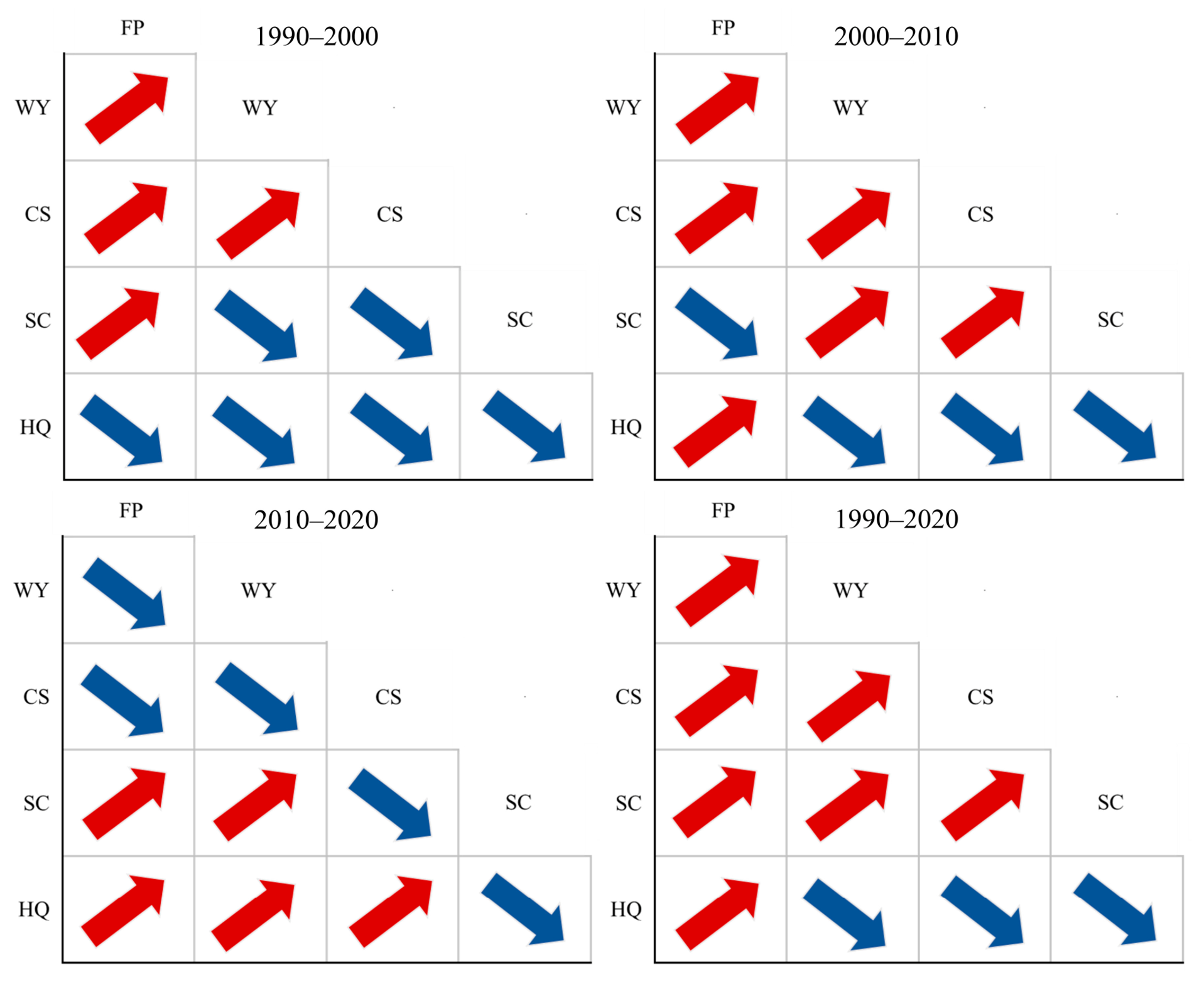
From the perspective of changes in regional ecosystem-service trade-offs and synergies (Figure 7), WY-FP, CS-FP, SC-FP, and CS-WY shifted toward stronger synergy during 1990–2000, whereas the other relationships shifted toward stronger trade-offs. During 2000–2010, SC-FP, HQ-WY, HQ-CS, and HQ-SC deteriorated toward stronger trade-offs, while the other relationships improved toward stronger synergy. During 2010–2020, the ratio of improving to deteriorating relationships was 1:1; SC-FP, SC-WY, HQ-FP, HQ-WY, and HQ-CS improved toward stronger synergy. Over the full 1990–2020 period, most ecosystem-service interactions improved toward synergy, with only HQ-WY, HQ-CS, and HQ-SC deteriorating toward trade-offs. Overall, trade-off and synergy relationships among ecosystem services are not static. Ecological protection and quality improvement should therefore account for ecosystem services and the interactions among different service functions in an integrated manner. The robustness tests showed that most ecosystem-service pairs had consistent signs and significance under Pearson, Spearman, and Kendall correlations. A small number of food-production-related pairs were sensitive to the correlation method, indicating that provisioning–regulating service relationships should be interpreted cautiously because food production is spatially concentrated and contains many zero-value cells.

3.4. Driving Factors of Land–Use Expansion and Ecosystem-Service Responses Under Different Development Scenarios

3.4.1. Contribution of Driving Factors to Land–Use Expansion

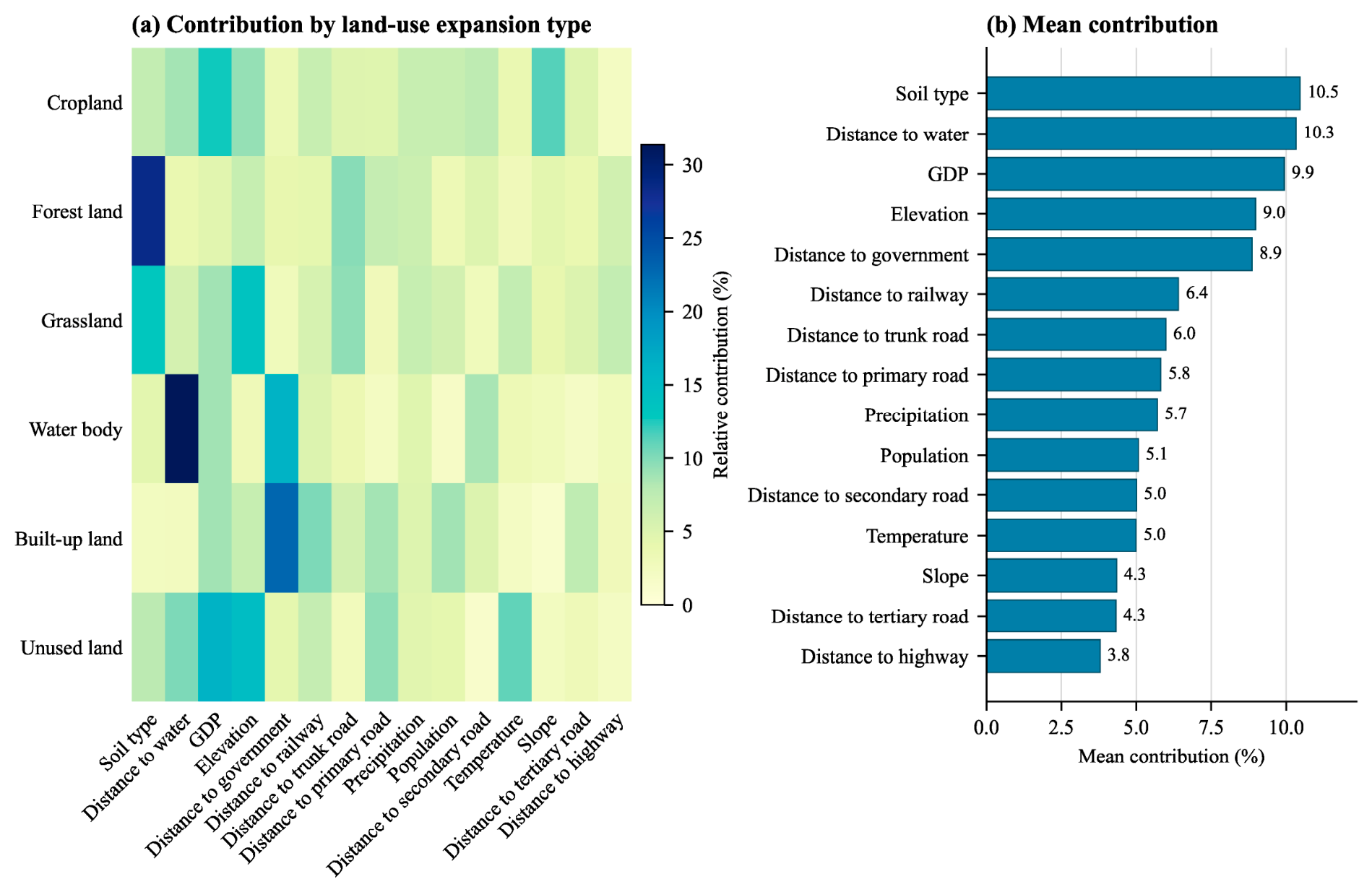
The PLUS-LEAS results show clear differences in the contribution of driving factors among land–use expansion types from 2010 to 2020 (Figure 8). In terms of the mean contribution across all six land–use types, soil type (10.46%), distance to water bodies (10.33%), GDP (9.94%), elevation (8.98%), and distance to government centers (8.86%) were the five most important factors. This indicates that land–use expansion in the UCS was jointly shaped by natural background conditions, water-resource constraints, socioeconomic development, and administrative-accessibility effects. Among different land–use types, forestland expansion was most strongly associated with soil type, water-body expansion was mainly controlled by distance to water bodies, and built-up land expansion was strongly influenced by distance to government centers, GDP, population, and road accessibility. Cropland and grassland expansion were influenced by both natural factors, such as soil type, elevation, and slope, and socioeconomic or accessibility factors. These results provide a quantitative explanation for why ecosystem-service supplies changed unevenly across space: the conversion and redistribution of land–use types, which directly determine InVEST inputs, were not random but were controlled by the combined effects of environmental suitability, water availability, and human development intensity.

3.4.2. Ecosystem Service Under Different Development Scenarios

Based on the PLUS model, the spatial distribution of land use in the UCS under different 2030 scenarios is predicted (Figure 9). Because the distribution of food production mainly depends on the spatial distributions of cropland and grassland, and these land–use patterns are projected to change only slightly under the three 2030 scenarios, the overall spatial pattern of food production is expected to remain similar to the historical pattern. High values will remain in the central oasis plain, whereas low values will occur in the northern and southern mountains and desert areas. Areas of food-supply change will continue to be concentrated around urban and rural settlements. Notably, high-value food-supply services increase substantially under the ecological-protection scenario. The overall distribution of water yield is similar to that in 2020, with a south-high/north-low pattern. It can be seen from

Table 1. Values of various ecosystem services under different scenarios.

Ecosystem Service	Metric	Unit	2020	BAU	ED	EP
Food production (FP)	Mean food production	t·km−2	62.06	62.03	62.03	64.59
Water yield (WY)	Mean water yield	mm	50.66	51.27	51.18	51.84
Water yield (WY)	Total water yield	108 m3	44.53	45.34	45.26	45.84
Carbon storage (CS)	Mean carbon storage	t·km−2	7467.93	7596.1	7577.42	7701.76
Carbon storage (CS)	Total carbon storage	109 t	10.57	10.75	10.73	10.9
Soil conservation (SC)	Mean soil conservation	t·km−2	1191.49	1304.41	1304.41	1305.82
Soil conservation (SC)	Total soil conservation	1010 t	10.7	11.7136	11.7136	11.7262
Habitat quality (HQ)	Mean habitat quality index	dimensionless	0.6583	0.6632	0.6626	0.6635

that under the BAU, ED, and EP scenarios, mean water-yield depths are 51.27, 51.18, and 51.84 mm, respectively, and total water yields are 45.34 × 10⁸, 45.26 × 10⁸, and 45.84 × 10⁸ m³, respectively. Compared with 2020, water yield changes only slightly and increases under all three scenarios, especially under EP. The spatial pattern of carbon storage is also largely consistent with that in 2020. High-value areas are concentrated in the southern and central areas with high vegetation cover, whereas low-value areas are located in the northern desert and Gobi areas with low vegetation cover. Under BAU, ED, and EP, mean carbon storage per unit area is 7596.10, 7577.42, and 7701.76 t·km⁻², and total carbon storage is 10.75 × 10⁹, 10.73 × 10⁹, and 10.90 × 10⁹ t, respectively. Both mean and total carbon storage increase relative to 2020, with the largest increase under EP and the smallest under ED. Soil conservation also increases slightly relative to 2020 under all three scenarios, with totals of 11.71 × 10¹⁰, 11.71 × 10¹⁰, and 11.73 × 10¹⁰ t. Soil conservation under ED is 4.67 ×10⁵ t lower than under BAU, whereas EP produces higher soil conservation than the other scenarios. The spatial pattern of habitat quality remains stable and shows a south-high/north-low distribution. The habitat-quality indices under the three scenarios are 0.6632, 0.6626, and 0.6635, respectively, indicating improvement relative to 2020. The EP scenario yields the best habitat-quality level among the three scenarios.

3.4.3. Trade-Offs and Synergies Among Ecosystem Services Under Different Development Scenarios

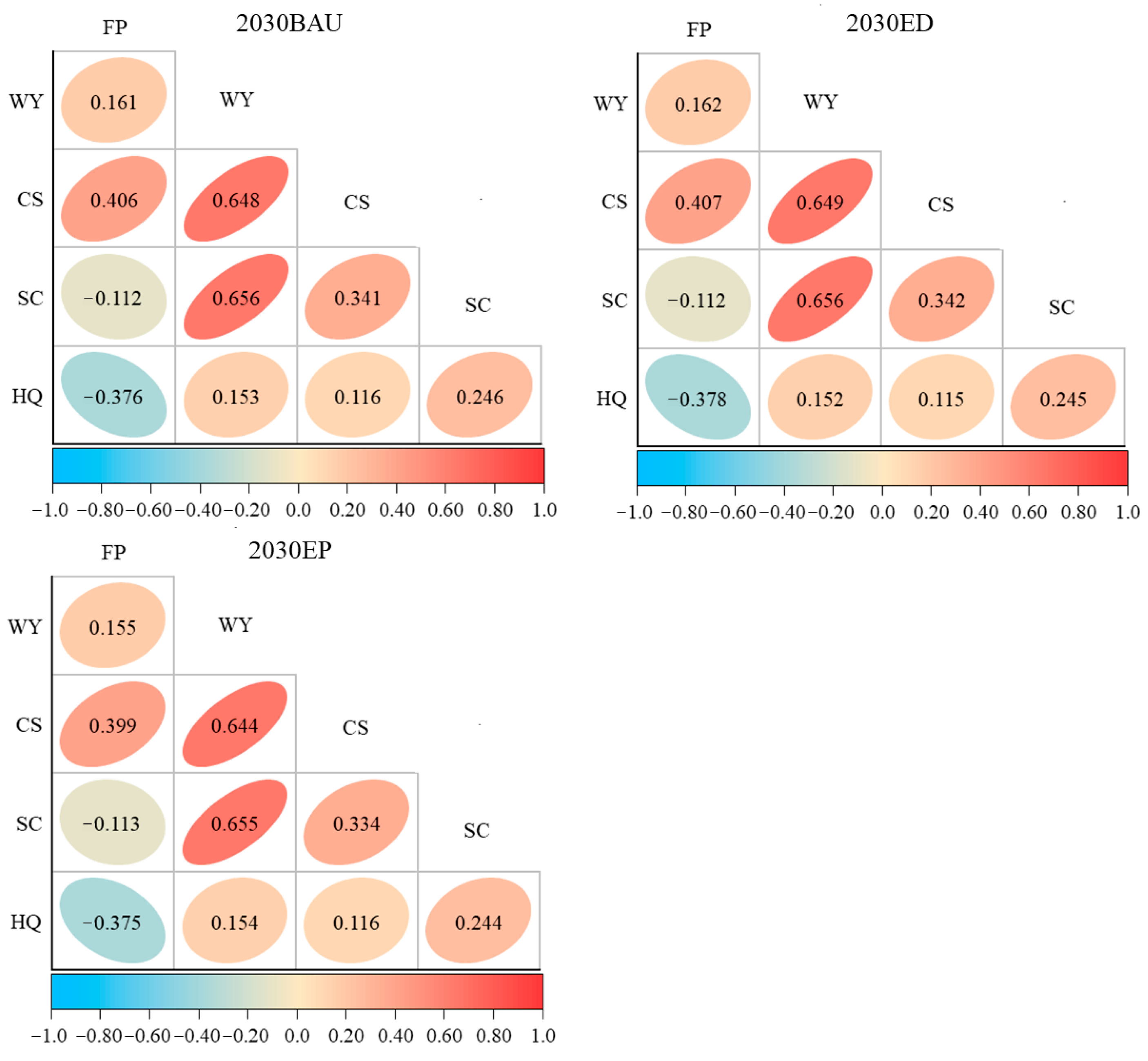
As shown in Figure 10, the directions of trade-off and synergy relationships among FP, WY, CS, SC, and HQ are consistent under all three scenarios. FP-WY, FP-CS, WY-CS, WY-SC, WY-HQ, CS-SC, CS-HQ, and SC-HQ show synergistic relationships, whereas FP-SC and FP-HQ show trade-offs. Under BAU, the SC-HQ synergy is relatively strong. Under ED, the FP-WY, FP-CS, WY-CS, and CS-SC synergies and the FP-HQ trade-off are relatively strong. Under EP, the WY-HQ synergy and the FP-SC trade-off are relatively strong.

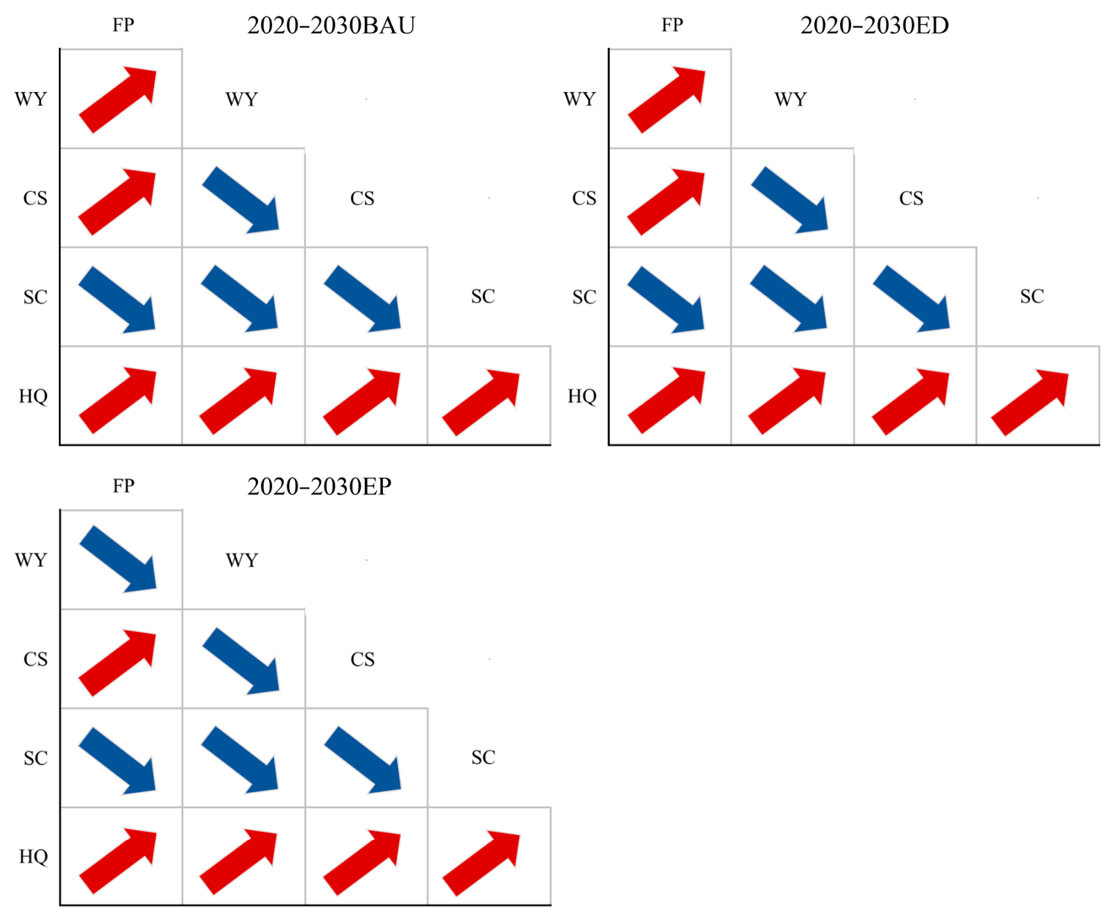
From the perspective of changes in trade-off and synergy relationships from 2020 to 2030 under different scenarios (Figure 11), the overall trends are similar. Under all three scenarios, FP-CS, FP-HQ, WY-HQ, CS-HQ, and SC-HQ shift toward stronger synergy, whereas FP-SC, WY-SC, WY-CS, and CS-SC shift toward stronger trade-offs. The FP-WY relationship shifts toward stronger synergy under BAU and ED but toward stronger trade-offs under EP.

4. Discussion

4.1. Interpretation and Implications of Ecosystem-Service Changes

The ES results show that land–use change in the UCS has not translated into uniform ecological improvement or degradation. Instead, provisioning services increased while water-, carbon-, soil-, and habitat-related services weakened, indicating a redistribution of ecosystem functions along the mountain–oasis–desert gradient. From 1990 to 2020, food production in the UCS increased markedly, while water yield, carbon storage, soil conservation, and habitat quality generally declined. This pattern is consistent with previous findings that agricultural intensification and oasis expansion can enhance provisioning services but may weaken regulating and supporting services in arid regions [43,44]. Similar water-resource constraints and water–land conflicts have also been reported in the Manas River Basin, where land–use change and irrigation expansion strongly affect ecosystem-service trade-offs [45,46]. The south-high/north-low spatial pattern of water yield, carbon storage, soil conservation, and habitat quality is also consistent with studies on the northern slope of the Tianshan Mountains and Xinjiang ecological zones, which emphasized the ecological importance of mountainous water-source areas and the vulnerability of the northern desert–oasis transition zone [47,48]. However, compared with watershed-scale studies, such as those on the Manas River Basin or Yili River Basin, the UCS shows stronger urban-agglomeration characteristics: high-intensity built-up land expansion, concentrated population and industry, and stronger conflicts among food production, water consumption, habitat conservation, and urban development. Therefore, this study not only confirms the existence of a widespread ecological gradient in arid Xinjiang but also reveals how this gradient interacts with urban agglomeration development, changes in landscape types, and future scenario pathways within the Urumqi–Changji–Shihezi-Wujiaqu oasis system.

4.2. Differentiated Contributions of Landscape Types to Ecosystem Services

This study evaluated food production by linking local agricultural and livestock statistics with NDVI-based spatial allocation. The results show that cropland remained the dominant food-production land type because grain, vegetable, and fruit production was concentrated in cultivated oasis areas. However, the contribution of grassland–related livestock products increased from 4.41% of terrestrial food production in 1990 to 10.19% in 2020. This increase occurred despite the reduction in grassland area, indicating that improvements in livestock breeding, disease prevention, forage utilization, and large-scale husbandry management enhanced the production efficiency of grassland–related food supply. Therefore, the food-production trend in the UCS reflects not only land–use change but also the adjustment of Xinjiang’s agricultural and animal husbandry structure. From 1990 to 2020, the mean water-yield depth of all land–use landscape types declined. Forestland, grassland, and cropland had high water-yield capacity, whereas built-up land had the lowest capacity. The differences in water-yield capacity among land types are similar to the findings of Wang et al. [49]. Because forestland, grassland, and cropland have relatively high vegetation cover and reduce evaporation, they have stronger water-yield capacity. Considering the area proportions of landscape types, grassland contributed the greatest total water yield, followed by cropland, forestland, unused land, water bodies, and built-up land. To address the decline in water-yield function in the south, the strategy of determining urban and greening scale according to water availability should be strictly implemented on the northern slope of the Tianshan Mountains, and expansion of high-water-consumption artificial forests should be restricted. In the central oasis agricultural area, water-saving technologies such as drip irrigation should be promoted while ensuring food security in order to reduce competition with water yield and habitat quality. Water bodies, built-up land, and unused land contributed little to carbon storage and showed little overall change. Cropland carbon storage increased, forestland carbon storage decreased, and grassland carbon storage first decreased and then increased; grassland contributed more than 60% of total regional carbon storage in all periods, consistent with the trend reported by Liu et al. [50]. These differences are jointly influenced by forest, grassland, and vegetation cover; spatial distribution; and area changes and transitions among land types. In addition, rapid urbanization has reduced forest and grassland area and vegetation cover, making it an important driver of overall carbon-storage decline. The capacity of water bodies, forestland, grassland, built-up land, cropland, and unused land to provide soil conservation differed, and total soil-conservation contributions varied markedly among landscape types. Comparisons with studies in regions with similar natural conditions indicate that soil conservation is crucial for supporting arid ecosystems [51,52,53]. Grassland, forestland, and water bodies contribute substantially to soil conservation in the UCS. Protection of water-source areas and key watersheds should therefore be strengthened, and returning cropland to forest and grassland should be implemented to increase vegetation cover, improve soil-conservation capacity, reduce soil erosion, and gradually restore regional soil-conservation services. Mean habitat-quality indices differed among land–use types, but habitat quality has changed only weakly over the past 30 years compared with other services and showed a slight overall decline. Rehman et al. evaluated habitat quality in the urban agglomeration on the northern slope of the Tianshan Mountains and found spatial heterogeneity [48], limited spatial change, and built-up-land expansion as the main cause of decline, consistent with this study. During socioeconomic development in the UCS, intensified human activities and threats from settlements, roads, railways, and cropland expansion have increased disturbance. Land–use transitions have reduced vegetation cover in some areas, further weakening ecological resistance to disturbance and affecting habitat quality.

Compared with previous studies that mainly evaluated ecosystem services at the administrative or watershed scale, the landscape-type contribution analysis in this study further clarifies the functional roles of cropland, grassland, forestland, water bodies, built-up land, and unused land in an arid oasis urban agglomeration. The results show that cropland is the core carrier of food production, grassland contributes substantially to water yield, carbon storage, and soil conservation because of its large area, and forestland and water bodies provide high unit-area regulating services but have a limited total contribution because of their smaller area. This finding refines the general conclusion of previous Xinjiang-scale studies by showing that ecosystem-service supply in the UCS depends not only on the ecological quality of each landscape type but also on its spatial extent and position within the mountain–oasis–desert system.

4.3. Dynamic Evolution of Trade-Offs and Synergies Among Ecosystem Services

The analysis of ecosystem-service trade-offs and synergies showed that the UCS has both similarities to and differences from other arid regions in Xinjiang. Previous studies in Kashgar, the Manas River Basin, and Xinjiang as a whole found that regulating and supporting services such as water yield, carbon storage, soil conservation, and habitat quality often show synergistic relationships, whereas provisioning services are more likely to trade off with ecological services [54]. The results of this study are generally consistent with this pattern, but the trade-off/synergy relationships in the UCS are more strongly shaped by urban-agglomeration development and oasis agriculture. In particular, the concentration of cropland and built-up land in the central oasis plain intensifies the competition between food production, water consumption, and habitat conservation, while the southern mountainous area maintains stronger synergies among water yield, carbon storage, soil conservation, and habitat quality. This indicates that ecosystem-service interactions in the UCS are not only ecological relationships but also reflect the spatial organization of oasis urbanization.

Furthermore, this study analyzed temporal changes in trade-off/synergy relationships and found that relationships among the five ecosystem services evolved dynamically across different periods. Future ecological protection and restoration should fully consider these dynamic interactions and implement differentiated and coordinated management to improve ecosystem services as a whole. This dynamic pattern indicates that restoration measures should not aim solely to maximize a single service; instead, dominant trade-offs should be identified at different development stages and regulated through coordinated management.

4.4. Comparison of Multi-Scenario Simulation Results and Identification of the Optimal Path

Scenario simulation has become an important method for linking land–use optimization with ecosystem-service management in arid regions. Previous PLUS-InVEST or CA–Markov–InVEST studies in Xinjiang and the Tarim River Basin have shown that ecological-protection scenarios generally help maintain carbon storage, habitat quality, and other regulating services [55,56]. Similar conclusions have also been reported in semi-arid urban areas, where ecological constraints can reduce the loss of ecosystem services under urban expansion [57]. The present study is consistent with these findings but differs in that it evaluates five ecosystem services simultaneously and compares BAU, ED, and EP pathways within the UCS oasis urban agglomeration. The results show that the EP scenario produces the most favorable overall ecosystem-service outcome, indicating that ecological constraints are particularly important in regions where urban expansion, agricultural production, and water-resource scarcity overlap. Based on projected land–use landscape distributions under different 2030 scenarios, this study further evaluated the five ecosystem-service functions in the UCS. Compared with 2020, BAU and ED produced slight increases in WY, CS, SC, and HQ, while FP remained almost unchanged and decreased marginally from 62.06 to 62.03 t km⁻². The EP scenario produced the most consistent improvement, increasing FP, WY, CS, SC, and HQ by approximately 4.08%, 2.33%, 3.13%, 9.60%, and 0.79%, respectively. Because landscape-type distribution is a key factor affecting ecosystem services, increases in ecological-function land, such as cropland, forestland, grassland, and water bodies, under EP lead to higher overall ecosystem-service levels than under the other scenarios. The limited differences between BAU and ED indicate that the short projection horizon and relatively stable land–use structure constrain the magnitude of ES change. The directions of trade-offs and synergies among ecosystem services remain consistent across the three scenarios, although their strengths differ slightly. Similar changes in ecosystem-service trends across scenarios lead to similar effects on trade-off and synergy relationships.

The ED and EP scenarios should be interpreted as policy-oriented sensitivity scenarios rather than deterministic forecasts. Their transition-probability adjustments were applied to the 2010–2020 historical transition matrix to represent different development pathways. The ED scenario emphasizes the expansion pressure of construction land under regional economic development, whereas the EP scenario emphasizes ecological conservation redlines, permanent basic farmland protection, water-source conservation, and ecological restoration. For arid oasis urban agglomerations, the principle of determining urban scale and land–development intensity according to water availability is particularly important. Therefore, reducing the conversion of cropland, forestland, and grassland to built-up or unused land and increasing the restoration of suitable unused land to ecological and agricultural land under EP are consistent with the spatial governance direction of ecological priority and high-quality development in Xinjiang. In contrast to the previous land–use study, where EP was evaluated mainly through changes in land categories, the present ES assessment shows why EP is ecologically preferable: it improves WY, CS, SC, and HQ while avoiding a decline in FP. Thus, its advantage lies in service coordination rather than in land–use structure alone. Under this scenario, strict delineation of ecological redlines, implementation of returning cropland to forest and grassland, and adherence to policies that determine urban scale, land use, population, and production according to water availability can effectively reduce trade-offs between food production and regulating services. Priority should be given to protecting water-yield areas in the southern mountains and the northern desert–oasis transition zone. Future planning should therefore prioritize compact urban renewal, protection of mountain water-source areas, restoration of desert–oasis transition zones, and a reduction in water–food–ecology competition in the central oasis.

Based on the spatial differentiation of ecosystem services and the functional positioning of different cities in the UCS, differentiated oasis-management strategies should be adopted. For Urumqi, which is the core metropolitan area, with the highest population density and built-up land intensity, priority should be given to compact urban development, strict control of construction-land expansion, protection of southern mountain water-source areas, restoration of urban ecological corridors, and improvement in water-use efficiency in urban greening. Large-scale expansion of high-water-consumption artificial green space should be avoided, and ecological restoration should focus on native drought-resistant vegetation and river-corridor connectivity. For Changji, which contains extensive oasis cropland and important agricultural production space, management should focus on permanent basic farmland protection, high-efficiency drip irrigation, groundwater control, a reduction in agricultural non-point source pollution, and ecological restoration of the desert–oasis transition zone. Cropland protection should be coordinated with habitat-quality improvement through farmland shelterbelts and ecological buffer zones. For Shihezi, which is characterized by intensive agricultural production and the Xinjiang Production and Construction Corps’ high-standard farmland system, the priority should be to improve agricultural water productivity, maintain shelterbelt networks, promote soil conservation and carbon sequestration in cropland and grassland, and control the outward expansion of construction land. Agricultural modernization should be linked with ecological compensation and low-carbon land management. For Wujiaqu, which is located in a sensitive oasis–desert transition area and has relatively limited ecological carrying capacity, urban expansion should be strictly constrained, ecological buffers should be strengthened, and restoration of degraded grassland, shelterbelts, wetlands, and desert-edge vegetation should be prioritized. These differentiated strategies can help balance food production, water-resource constraints, habitat conservation, and urban development within the UCS.

4.5. Limitations and Prospects

This study still has several limitations and uncertainties. First, because long-term consistent geospatial datasets are difficult to obtain, this study used 30 m land–use data and unified the ecosystem-service assessment to a 250 m spatial resolution. These data are sufficient for identifying regional-scale landscape-pattern evolution and ecosystem-service trends, but they cannot fully capture fine-scale heterogeneity in irrigation canals, shelterbelts, small wetlands, aquaculture ponds, orchards, urban green spaces, and desert–oasis transition zones. Future studies should integrate higher-resolution remote-sensing images, field observations, irrigation-network data, orchard distribution data, aquaculture statistics, and urban green-space datasets to improve ecosystem-service assessment at the plot, city, and oasis-edge scales.

Second, uncertainties remain in the InVEST-based ecosystem-service assessment. The InVEST model is widely used for spatially explicit ecosystem-service evaluation, but its outputs are sensitive to model parameters such as carbon density, vegetation evapotranspiration coefficients, root depth, soil erodibility, rainfall erosivity, habitat threat weights, habitat sensitivity coefficients, and half-saturation constants. In this study, key parameters were localized using regional climatic, soil, vegetation, hydrological, statistical, and land–use data, and complete parameter tables are provided in the Supplementary Materials to improve transparency and reproducibility. Nevertheless, because field observations for all parameters remain limited, the model outputs should be interpreted mainly as indicators of regional spatiotemporal patterns and relative changes rather than precise site-level quantities.

Third, the future scenarios in this study were mainly driven by PLUS-simulated land–use change, while future climate change was not dynamically coupled with the InVEST modules. This design helps isolate the ecosystem-service effects of different land–use pathways, but it may underestimate the influence of future precipitation, temperature, evapotranspiration, snow and glacier meltwater, and drought-frequency changes in arid oasis regions. Therefore, the 2030 scenario results should be interpreted as land–use-policy-driven projections under the current climate-background assumption. Future research should couple PLUS-based land–use scenarios with CMIP6 climate pathways, such as SSP2-4.5 and SSP5-8.5, and update precipitation, reference evapotranspiration, vegetation, and hydrological inputs in the InVEST model to assess the combined effects of land–use change and climate change.

Fourth, Pearson correlation coefficients were used to identify the overall direction and relative strength of trade-offs and synergies among ecosystem services. However, ecosystem-service maps exhibit spatial autocorrelation, and global Pearson coefficients may overestimate statistical significance and mask local spatial heterogeneity. Therefore, the correlation results in this study should be interpreted primarily as regional-scale association indicators rather than independent-sample inferential statistics or local spatial-clustering results. Because this study focused on long-term temporal changes, landscape-type contributions, and multi-scenario responses, grid-level local correlation and hotspot mapping were not included as core analyses. Future work should apply spatially explicit methods, such as LISA, Getis-Ord Gi*, geographically weighted correlation, spatial regression, or copula-based approaches, to reveal local trade-off/synergy clusters, nonlinear relationships, and scale-dependent mechanisms.

Fifth, although the LEAS module quantified the contribution of driving factors to land–use expansion, this analysis mainly explains the land–use pathway through which external drivers affect ecosystem-service patterns, rather than the independent causal effect of each factor on each ecosystem-service indicator. Future studies could combine PLUS-LEAS with spatial attribution methods, such as Geodetector, XGBoost-SHAP, or structural equation modeling, to directly quantify the nonlinear and interactive effects of climate change, socioeconomic development, accessibility, and policy constraints on ecosystem-service supply.

Finally, this study mainly evaluated the supply side of ecosystem services and did not systematically quantify ecosystem-service demand or supply-demand matching. In arid oasis urban agglomerations, ecological pressure depends not only on ecosystem-service supply capacity but also on demand from population concentration, food consumption, agricultural irrigation, industrial water use, carbon-emission reduction targets, and ecological recreation. Future research should integrate ecosystem-service supply with population density, water-resource demand, food demand, carbon-neutrality targets, industrial and agricultural water demand, and accessibility to ecological spaces to construct supply-demand balance maps. This would help identify ecosystem-service deficit areas, clarify cross-regional ecological compensation relationships, and support more precise differentiated management in Urumqi, Changji, Shihezi, and Wujiaqu.

5. Conclusions

Building on land–use and scenario information for the UCS, this study assessed how five ecosystem services changed, which landscape types carried these services, and how service relationships responded to alternative 2030 land–use pathways. The main conclusions are as follows:

(1) From 1990 to 2020, regional food production generally increased, whereas water yield, carbon storage, soil conservation, and habitat quality decreased. Water yield, carbon storage, soil conservation, and habitat quality showed south-high/north-low spatial patterns and clear elevation-related zonation. (2) The distribution of land–use landscape types influenced the strength of ecosystem-service capacity, and the area of each landscape type further affected total ecosystem-service supply. (3) Ecosystem services showed trade-offs and synergies to different degrees. Trade-offs and synergies among the five services were dynamic and shifted toward either stronger trade-offs or stronger synergies in different periods. (4) The PLUS-LEAS analysis showed that soil type, distance to water bodies, GDP, elevation, and distance to government centers were the dominant driving factors of land–use expansion from 2010 to 2020, indicating that ecosystem-service changes were indirectly regulated by the combined effects of natural suitability, water-resource constraints, and socioeconomic accessibility through land–use change. (5) Under different development scenarios, food production, water yield, carbon storage, soil conservation, and habitat quality in the UCS increased to varying degrees compared with 2020, with more pronounced increases under the ecological-protection scenario. Although the strength of ecosystem-service trade-offs and synergies fluctuated among scenarios, the underlying mechanisms and directions of their interactions remained highly consistent.

The results demonstrate that integrating long-term ecosystem-service assessment, landscape-type contribution analysis, trade-off/synergy identification, and PLUS-based scenario simulation can provide a refined decision-support framework for arid oasis urban agglomerations. For the UCS, ecosystem-service optimization should not rely on a single regional strategy; instead, differentiated management should be implemented for Urumqi, Changji, Shihezi, and Wujiaqu according to their urban-development intensity, agricultural function, water-resource constraints, and ecological carrying capacity. However, future studies should further couple land–use scenarios with climate-change pathways, quantify parameter sensitivity and uncertainty, and incorporate ecosystem-service demand to improve the policy applicability of ecosystem-service optimization in arid oasis urban agglomerations.

References

1. Zhang, J.; Wang, M.; Liu, K.; Chen, S.; Zhao, Z. Social-ecological system sustainability in China from the perspective of supply-demand balance for ecosystem services. J. Clean. Prod. 2025, 497, 145039. [Google Scholar]
2. Liu, Y.; Wang, J.; Ding, J.; Zhang, Z.; Liu, Z.; Zhang, Z.; Zhang, J.; Shi, L. Dynamic Monitoring of Ecological Environmental Quality in Arid and Semi-Arid Regions: Disparities Among Central Asian Countries and Analysis of Key Driving Factors. Remote Sens. 2025, 17, 1825. [Google Scholar] [CrossRef] [Scilit]
3. Li, X.; Zhang, L.; Guo, H.; Fu, W.; Lu, L.; Qiu, Y.; Wang, X.; Jia, G. Space recognition of eco-environment global change response of arid and semi-arid region of the Silk Road Economic Belt. Bull. Chin. Acad. Sci. 2016, 31, 559–566. [Google Scholar]
4. Jiang, J.; Abulizi, A.; Abliz, A.; Zayiti, A.; Akbar, A.; Ou, B. Construction of landscape ecological security pattern in the Zhundong region, Xinjiang, NW China. Int. J. Environ. Res. Public Health 2022, 19, 6301. [Google Scholar] [CrossRef] [Scilit] [PubMed]
5. Bi, J.; Lu, M.; Liu, F.; Cai, Y.; Wang, Y.; Duan, M.; Li, J.; Li, X.; Yu, D. Multi-scale urban ecosystem service changes and their impact mechanisms on human well-being. J. Environ. Manag. 2025, 374, 124117. [Google Scholar] [CrossRef] [Scilit]
6. Liu, M.; Wie, H.; Dong, X.; Wang, X.; Zhao, B.; Zhang, Y. Integrating land use, ecosystem service, and human well-being: A systematic review. Sustainability 2022, 14, 6926. [Google Scholar] [CrossRef] [Scilit]
7. Shoyama, K.; Kamiyama, C.; Morimoto, J.; Ooba, M.; Okuro, T. A review of modeling approaches for ecosystem services assessment in the Asian region. Ecosyst. Serv. 2017, 26, 316–328. [Google Scholar] [CrossRef] [Scilit]
8. Wu, Q.; Cao, Y.; Zhang, Y.; Su, D.; Fang, X. Linking ecosystem services trade-offs, human preferences and future scenario simulations to ecological security patterns: A novel methodology for reconciling conflicting ecological functions. Appl. Geogr. 2025, 176, 103534. [Google Scholar] [CrossRef] [Scilit]
9. Zandebasiri, M.; Goujani, H.; Iranmanesh, Y.; Azadi, H.; Viira, A.H.; Habibi, M. Ecosystem services valuation: A review of concepts, systems, new issues, and considerations about pollution in ecosystem services. Environ. Sci. Pollut. Res. 2023, 30, 83051–83070. [Google Scholar] [CrossRef] [Scilit]
10. Woodman, T.L.; Alexander, P.; Burslem, D.F.R.P.; Travis, J.M.J.; Winkler, K.; Eigenbrod, F. Global assessment of landscape pattern changes from 1992 to 2020. Landsc. Ecol. 2025, 40, 196. [Google Scholar] [CrossRef] [Scilit] [PubMed]
11. Jia, Q.; Jiao, L.; Lian, X.; Wang, W. Linking supply-demand balance of ecosystem services to identify ecological security patterns in urban agglomerations. Sustain. Cities Soc. 2023, 92, 104497. [Google Scholar] [CrossRef] [Scilit]
12. Schlutow, A.; Schröder, W. Rule-based classification and mapping of ecosystem services with data on the integrity of forest ecosystems. Environ. Sci. Eur. 2021, 33, 50. [Google Scholar] [CrossRef] [Scilit]
13. Cheng, Y.; Kang, Q.; Liu, K.; Cui, P.; Zhao, K.; Li, J.; Ma, X.; Ni, Q. Impact of urbanization on ecosystem service value from the perspective of spatio-temporal heterogeneity: A case study from the Yellow River Basin. Land 2023, 12, 1301. [Google Scholar] [CrossRef] [Scilit]
14. Xin, J.; Wang, D.; Wang, Y.; Tan, Y.; Zheng, J.; Xu, X.; Lu, Y.; Huang, W.; Wie, Z.; Zhang, H.; et al. A hierarchical-modular ecosystem mapping framework for high-intensity human activity zones. Int. J. Digit. Earth 2025, 18, 2564468. [Google Scholar] [CrossRef] [Scilit]
15. Yang, L.; Zhou, X.; Gu, X.; Liang, Y. Impact mechanism of ecosystem services on resident well-being under sustainable development goals: A case study of the Shanghai metropolitan area. Environ. Impact Assess. Rev. 2023, 103, 107262. [Google Scholar] [CrossRef] [Scilit]
16. Qiu, J.; Yu, D.; Huang, T. Influential paths of ecosystem services on human well-being in the context of the sustainable development goals. Sci. Total Environ. 2022, 852, 158443. [Google Scholar] [CrossRef] [Scilit] [PubMed]
17. Guo, T.; Wu, S.; Zhang, X.; Zhang, C.; Yang, J.; Cheng, S. Measurement and Influencing Factors of Willingness to Accept Payment for Ecosystem Service Provision: A Case Study of a Leading Forest Farm in China. Forests 2023, 14, 2417. [Google Scholar] [CrossRef] [Scilit]
18. Li, M.; Zhu, J.; Dong, H. A study on the impact of watershed compensation policies on green technology innovation ecosystems. Systems 2025, 13, 44. [Google Scholar] [CrossRef] [Scilit]
19. Li, Z.; Zhou, Z.; Liu, Z.; Si, J.; Ou, J. Assessment and Dynamic Prediction of Green Space Ecological Service Value in Guangzhou City, China. Remote Sens. 2024, 16, 4180. [Google Scholar] [CrossRef] [Scilit]
20. Cheng, A.; Zhang, M.; Wang, Y. Who gets the green? Daily mobility and unequal exposure to urban green space among adolescents in China. Urban For. Urban Green. 2025, 112, 128960. [Google Scholar] [CrossRef] [Scilit]
21. Van, O.W.; Van, P.S.; Cools, J. Urban green infrastructure: A review on valuation toolkits from an urban planning perspective. J. Environ. Manag. 2020, 267, 110603. [Google Scholar] [CrossRef] [Scilit]
22. Chen, H. Establishment and application of wetlands ecosystem services and sustainable ecological evaluation indicators. Water 2017, 9, 197. [Google Scholar] [CrossRef] [Scilit]
23. Fang, J.; Xu, L.; Lu, Q. Ecological security patterns of Chinese lakes based on ecosystem service values assessment and human threat factors evaluation. Ecol. Inform. 2024, 82, 102754. [Google Scholar] [CrossRef] [Scilit]
24. Zhang, Z.; He, Z.; Su, K.; Wu, S.; Liu, L. Global evolution of ecosystem services research in watersheds: Insights from large language models. Land Use Policy 2026, 160, 107849. [Google Scholar] [CrossRef] [Scilit]
25. Ran, P.; Frazier, A.E.; Xia, C.; Tiando, D.S.; Feng, Y. How does urban landscape pattern affect ecosystem health? Insights from a spatiotemporal analysis of 212 major cities in China. Sustain. Cities Soc. 2023, 99, 104963. [Google Scholar] [CrossRef] [Scilit]
26. García-Pardo, K.A.; Moreno-Rangel, D.; Domínguez-Amarillo, S.; Garcia-Chavez, J.R. Remote sensing for the assessment of ecosystem services provided by urban vegetation: A review of the methods applied. Urban For. Urban Green. 2022, 74, 127636. [Google Scholar] [CrossRef] [Scilit]
27. Ma, Y.; Yang, J. A review of methods for quantifying urban ecosystem services. Landsc. Urban Plan. 2025, 253, 105215. [Google Scholar] [CrossRef] [Scilit]
28. Li, Q.; Li, D.; Wang, J.; Wang, R.; Fu, G.; Yuan, Y.; Zheng, Z. Spatial heterogeneity of ecosystem service bundles and the driving factors in the Beijing-Tianjin-Hebei region. J. Clean. Prod. 2024, 479, 144006. [Google Scholar] [CrossRef] [Scilit]
29. Li, S.; Li, R.; Wang, L.; Fu, M.; Tian, Y.; Zhang, J. Study on the multi-scale characteristics of ecosystem service trade-offs, synergies and ecosystem service bundles in Beijing. Environ. Earth Sci. 2025, 84, 359. [Google Scholar] [CrossRef] [Scilit]
30. Xinjiang Uygur Autonomous Region Bureau of Statistics. Xinjiang Statistical Yearbook (2021); China Statistics Press: Beijing, China, 2021.
31. Xinjiang Production and Construction Corps Bureau of Statistics. Statistical Yearbook of Xinjiang Production and Construction Corps (2021); China Statistics Press: Beijing, China, 2021.
32. Gan, L.; Halik, Ü.; Shi, L.; Ru, J.; Wie, Z.; Li, J.; Welp, M. Integrating Multi-Source Data to Explore Spatiotemporal Dynamics and Future Scenarios of Arid Urban Agglomerations: A Geodetector–PLUS Modelling Framework for Sustainable Land Use Planning. Remote Sens. 2025, 17, 1851. [Google Scholar] [CrossRef] [Scilit]
33. Quarmby, N.A.; Milnes, M.; Hindle, T.L.; Silleos, N. The Use of Multi-Temporal NDVI Measurements from AVHRR Data for Crop Yield Estimation and Prediction. Int. J. Remote Sens. 1993, 14, 199–210. [Google Scholar] [CrossRef] [Scilit]
34. Gong, J.; Liu, D.; Gao, B.; Xu, C.; Li, Y. Tradeoffs and synergies of ecosystem services in western mountainous China: A case study of the Bailongjiang watershed in Gansu, China. Chin. J. Appl. Ecol. 2020, 31, 1278–1288. [Google Scholar]
35. Tallis, H.T.; Ricketts, T.; Guerry, A.D.; Nelson, E.; Ennaanay, D.; Wolny, S.; Olwero, N.; Vigerstol, K.; Pennington, D.; Mendoza, G.; et al. InVEST 2.1 Beta User’s Guide; The Natural Capital Project: Stanford, CA, USA, 2011. [Google Scholar]
36. Zhao, M.; He, Z.; Du, J.; Chen, L.; Lin, P.; Fang, S. Assessing the effects of ecological engineering on carbon storage by linking the CA-Markov and InVEST models. Ecol. Indic. 2019, 98, 29–38. [Google Scholar] [CrossRef] [Scilit]
37. Chen, X.; Yu, L.; Du, Z.; Xu, Y.; Zhao, J.; Zhao, H.; Zhang, G.; Peng, D.; Gong, P. Distribution of ecological restoration projects associated with land use and land cover change in China and their ecological impacts. Sci. Total Environ. 2022, 825, 153938. [Google Scholar] [CrossRef] [Scilit] [PubMed]
38. Liu, J.; Xi, L.; Zhang, R.; Zhang, B. A study on simulation and prediction of ecosystem service value in Jilin Province based on CA-Markov and InVEST model. Bull. Soil Water Conserv. 2020, 40, 153–159+329–330. [Google Scholar]
39. Zhao, J.; Li, C. Investigating spatiotemporal dynamics and trade-off/synergy of multiple ecosystem services in response to land cover change: A case study of Nanjing city, China. Environ. Monit. Assess. 2020, 192, 701. [Google Scholar] [CrossRef] [Scilit] [PubMed]
40. Zar, J.H. Biostatistical Analysis; Pearson Education India: Noida, India, 1999. [Google Scholar]
41. Dormann, C.F.; Elith, J.; Bacher, S.; Buchmann, C.; Carl, G.; Carré, G.; García Marquéz, J.R.; Gruber, B.; Lafourcade, B.; Leitão, P.J.; et al. Collinearity: A review of methods to deal with it and a simulation study evaluating their performance. Ecography 2013, 36, 27–46. [Google Scholar]
42. Liang, X.; Guan, Q.; Clarke, K.C.; Liu, S.; Wang, B.; Yao, Y. Understanding the drivers of sustainable land expansion using a patch-generating simulation (PLUS) model: A case study in Wuhan, China. Comput. Environ. Urban Syst. 2021, 85, 101569. [Google Scholar] [CrossRef] [Scilit]
43. Li, Z. Study on the Spatiotemporal Coupling Relationship Between Urbanization and Ecosystem Services in the North Slope Economic Belt of the Tianshan Mountains. Master’s Thesis, Shihezi University, Shihezi, China, 2023. [Google Scholar]
44. Wang, Y.; Ding, J.; Li, X.; Zhang, J.; Ma, G. Impact of LUCC on ecosystem services values in the Yili River Basin based on an intensity analysis mode. Acta Ecol. Sin. 2022, 42, 3106–3118. [Google Scholar] [CrossRef] [Scilit]
45. Yin, L.; Xu, X.; Hu, B.; Liu, L.; Wang, X.; Jia, H. The driving factors of ecosystem services and their tradeoffs in the Manas River basin of Xinjiang, China. J. Agric. Resour. Environ. 2024, 41, 1157–1170. [Google Scholar]
46. Du, Y. Study on the Assessment of Ecosystem Service Functions in the Manas River Basin. Master’s Thesis, Shihezi University, Shihezi, China, 2023. [Google Scholar]
47. Zhang, Z.R. Study on the Trade-off and Synergy and Driving Factors of Key Ecosystem Service in Xinjiang. Master’s Thesis, Chinese Research Academy of Environmental Sciences, Beijing, China, 2023. [Google Scholar]
48. Rehman, K.; Kasim, A.; Ablat, H.; Dolati, S.; Xu, J. Research on the temporal and spatial Evolution of habitat quality in urban agglomeration on the Northern Slope of Tianshan Mountains based on InVEST model. J. Ecol. Rural Environ. 2022, 38, 1112–1121. [Google Scholar]
49. Wang, X.; Chen, C.; Yin, L.; Feng, X.; Wie, X. Spatial-temporal changes and tradeoff/synergy relationship of ecosystem services in Xinjiang. Chin. J. Ecol. 2020, 39, 990–1000. [Google Scholar]
50. Liu, Y.; Yuan, X.; Li, J.; Qian, K.; Yan, W.; Yang, X.; Ma, X. Trade-offs and synergistic relationships of ecosystem services under land use change in Xinjiang from 1990 to 2020: A Bayesian network analysis. Sci. Total Environ. 2023, 858, 160015. [Google Scholar] [CrossRef] [Scilit] [PubMed]
51. Zhu, Q.; Wu, W.; Wang, Z.; Wang, T. Spatiotemporal coupling and coordination of ecosystem services and water-energy-food system security in Xinjiang. Arid Zone Res. 2026, 43, 176. [Google Scholar]
52. Yang, S.; Cui, X. Characteristics of spatiotemporal changes in ecosystem services in Xinjiang ecological zones. Clim. Environ. Res. 2024, 29, 302–316. [Google Scholar]
53. Hu, W.; Liu, W.; Peng, Y. Vegetation cover dynamics of Xinjiang grassland under grassland ecological restoration project and its constraining effects on ecosystem services. J. Soil Water Conserv. 2025, 39, 202–214+223. [Google Scholar]
54. Guo, L. The Study on Trade-Offs of Ecosystem Services in Kashgar Region, Xinjiang Based on Land Use. Master’s Thesis, Shihezi University, Shihezi, China, 2022. [Google Scholar]
55. Fu, K.; Jia, G.; Yu, X.; Chen, X. Analysis of temporal and spatial carbon stock changes and driving mechanism in Xinjiang Region by coupled PLUS-InVEST-Geodector model. Environ. Sci. 2024, 45, 5416–5430. [Google Scholar]
56. Fu, W.; Xia, W.; Fan, T.; Zou, Z.; Huo, Y. Scenario projection analysis of ecosystem carbon stocks in the Tarim River Basin. Arid Land Geogr. 2024, 47, 634–647. [Google Scholar]
57. Zhao, X.; Gao, Y.; Liu, Y.; Liu, L. Modeling trade-offs and synergies among ecosystem services in response to multi-scenario land use in a semi-arid city. Resour. Sci. 2025, 47, 2365–2379. [Google Scholar] [CrossRef] [Scilit]
Figure 1. Research framework of the study.
Land 15 01267 g001
Figure 2. Location of the study area.
Land 15 01267 g002
Figure 3. Comparison between the observed and PLUS-simulated land–use distributions in the UCS in 2020.
Land 15 01267 g003
Figure 4. The spatial pattern of ecosystem services in the UCS from 1990 to 2020. (a) Food-production service; (b) water-yield service; (c) carbon-storage service; (d) soil-conservation service; (e) habitat-quality service.
Land 15 01267 g004
Figure 5. Change trends of ecosystem services across different land–use types in the UCS. (a) Food production; (b) average depth of water production; (c) total water supply; (d) carbon storage; (e) soil conservation; and (f) habitat quality.
Land 15 01267 g005
Figure 6. The trade-offs and synergies between different ecosystem services in the UCS from 1990 to 2020 (p < 0.01, FP = food production, WY = water yield, CS = carbon storage, SC = soil conservation, HQ = habitat quality).
Land 15 01267 g006
Figure 7. Trends in the trade-off and synergy relationships of ESs in the UCS from 1990 to 2020.
Land 15 01267 g007
Figure 8. Relative contributions of driving factors to land–use expansion from 2010 to 2020 based on the PLUS-LEAS module. (a) Contributions by land–use expansion type; (b) mean contribution across the six land–use expansion types.
Land 15 01267 g008
Figure 9. The distribution of ecosystem services under different scenarios in the UCS in 2030. (a) Food-production service; (b) water-yield service; (c) carbon-storage service; (d) soil-conservation service; (e) habitat-quality service.
Land 15 01267 g009
Figure 10. The trade-offs and synergies among ESs under different scenarios in the UCS in 2030 (p < 0.01, FP = food production, WY = water yield, CS = carbon storage, SC = soil conservation, HQ = habitat quality).
Land 15 01267 g010
Figure 11. Changes in trade-off and synergy relationships among ecosystem services from 2020 to 2030 under different scenarios.
Land 15 01267 g011