


Abstract
The Arctic is warming nearly four times faster than the global mean, driving unprecedented sea ice loss and threatening permafrost coasts and human settlements. Existing pan-Arctic vulnerability indices typically rest on satellite-era baselines and on expert-driven weighting schemes whose robustness is rarely tested. Here, we present an integrated, multi-centennial framework that jointly ingests SIBT1850 sea ice concentration (1850–2017), extended to 2024 with the NOAA/NSIDC Climate Data Record of Passive Microwave Sea Ice Concentration v6 (G02202 v6), together with ESA CCI Permafrost products (1997–2019), the Arctic Coastal Dynamics database, and pan-Arctic settlement inventories. Using non-parametric Mann–Kendall trend tests, Sen’s slope, and the Pettitt change point test across nine Seas (S1–S9), five permafrost-adjacent core seas exhibit summer Sen’s slopes of −0.105 to −0.185% yr−1 with Pettitt change points clustered in 1929–1953 (mean 1936), whereas three of four support seas cluster around 1978, suggesting an approximately bimodal regime shift timing that we interpret cautiously given the limited sample. A Composite Vulnerability Index integrating six normalised indicators identifies the Chukchi (CVI = 0.630) and East Siberian (0.624) seas as the highest-priority hotspots at the SIBT1850 baseline. A satellite-era robustness check using NSIDC G02202 v6 confirms that the Chukchi–East Siberian–Laptev corridor remains in the top three highest-vulnerability basins under the 1850–2024 extension, with the Beaufort Sea retaining rank 5, validating the basin mean conclusions of the SIBT1850-based analysis. Robustness checks—PCA re-weighting, one-at-a-time and global (Sobol, PAWN) sensitivity analyses, and Monte Carlo Dirichlet perturbation—confirm that the top-two ranking is stable across weighting schemes (baseline–PCA Spearman ρ = 0.80). We explicitly avoid claiming forecasting validation, operational testing, or benchmarking against existing pan-Arctic vulnerability indices, all of which we identify as priority directions for future work. The framework provides a transparent, reproducible basis for prioritising adaptation across the Chukchi–East Siberian–Laptev corridor.
1. Introduction and Conceptual Framework
1.1. Arctic Amplification and the Coupled Cryosphere–Coastal System
The Arctic is undergoing the most rapid environmental transformation on Earth. Multiple datasets demonstrate that Arctic near-surface temperatures have risen approximately four times faster than the global mean since 1979–1980, an amplification greater than traditionally reported and systematically underestimated by climate models, likely because models under-represent feedbacks between sea ice loss and atmospheric temperatures [1,2,3]. Internal variability has further inflated the observed amplification by approximately 38% relative to the externally forced signal, making a fourfold ratio an extremely rare event in model simulations [3,4], with one analysis suggesting amplification peaked in the early 2000s, coincident with maximum sea ice loss rates [5]. Remote-sensing-based syntheses further confirm an alarming pan-Arctic ice cover recession over recent decades [6].
This warming is most clearly expressed in the rapid retreat of Arctic sea ice. Passive microwave records since 1979 show September extent declining at roughly 13.3% decade−1 during 1979–2014 [7,8,9] and 12.8% decade−1 during 1979–2018, with the 12 lowest extents occurring in the last 12 years of that record [9]. Sea ice has thinned dramatically, with September 2018 volume roughly three times lower than in 1979 and multi-year ice greatly reduced [7,9,10,11]; these trends are widely regarded as among the clearest global climate change signals [10,11,12]. Sea ice loss enhances Arctic amplification through ice–albedo and other feedbacks [9,11,13,14], with especially strong impacts in the western Arctic Ocean [11,14]. Consequences include increased coastal erosion due to longer open-water fetch and warmer waters, changes in precipitation type that harm terrestrial herbivores, and stress on ice-dependent marine mammals [11,13]. In permafrost-adjacent shelves such as the Chukchi Sea, biomarker records document a shift from extensive late-19th-century ice to marginal ice zone conditions since the 1930s, with sustained retreat and rising terrigenous input and stratification since the 1990s [14].
1.2. Long-Term Sea Ice Reconstructions and Pre-Satellite Context
Reconstructions extend this picture back well before the satellite era. The SIBT1850 database provides monthly, pan-Arctic sea ice extent and concentration since 1850 [8], showing that neither the recent minimum extent nor the post-1990s retreat rate has precedent on a pan-Arctic scale, with especially rapid loss in the Beaufort and Chukchi Seas [8]. A gridded reconstruction (1850–2018) reveals a substantial early-20th-century loss of approximately 1.25 × 10⁶ km2 during 1910–1940, with 25-year trends 33–38% smaller than the satellite-era trend but nearly twice earlier estimates, and decadal variability before satellites approximately 40% larger than previously thought [15]. An extended September series (1935–2014) finds positive trends until the early 1980s, with strongly negative significant trends only after about 2006 [16]. A multi-proxy reconstruction over the last 1450 years concludes that the duration and magnitude of the recent summer sea ice decline are unprecedented, linking multidecadal changes mainly to warm Atlantic inflow [17], and reviews emphasise the relative stability of pan-Arctic extents over past millennia until pronounced decline began in the late 1970s [18]. Reconstructions and reviews further highlight pronounced regional differences, with some sectors (e.g., Beaufort/Chukchi) showing exceptional recent retreat and others more variable [8,12,14,18].
Because pre-satellite reconstructions necessarily integrate heterogeneous observational sources, cross-comparison between independent products is important. In the Barents–Kara sector, SIBT1850 has been shown to be more realistic than HadISST1 in the pre-satellite era when evaluated against temperature-based proxies [19]; differences between the two products are mostly confined to the early 20th century and to high-summer months, when ship-based observations are sparse. We use SIBT1850 as the primary multi-centennial record and refer to HadISST1 [20] for pre-satellite context. To address concerns regarding the temporal currency of the analysis, we further extend the satellite-era portion of the record to 2024 with the NOAA/NSIDC Climate Data Record of Passive Microwave Sea Ice Concentration v6 (G02202 v6) [21]; this extension is described in Section 2.1 and reported in detail in Appendix B as a satellite-era robustness check. The PIOMAS-based volume reconstruction [22] supplies additional thermodynamic context.
1.3. From Sea Ice Loss to Permafrost Coastal Erosion: A Mechanistic Process Chain
Sea ice loss is tightly coupled to terrestrial change along permafrost coasts. The marine cryosphere influences coastal land system change through a multi-step physical chain in which (i) reduced summer sea ice concentration lengthens the open-water season, (ii) a longer open-water season enlarges the effective wave fetch at any given storm event, (iii) larger fetch and warmer near-shore waters increase wave energy delivered to ice-rich permafrost bluffs, and (iv) the combined action of warm water thermo-abrasion and air- and insolation-driven thermo-denudation produces bluff retreat and land loss [23,24,25,26,27]. Modelling and observations along the Beaufort coast show that erosion rates tripled as the sea-ice-free season roughly doubled from approximately 45 to 100 days, with about 40% of annual erosion occurring during less than 5% of the open-water season [27]. A fetch-limited wave model for northern Alaska links reduced sea ice cover directly to a 2.5-fold increase in exposure of permafrost bluffs to wave action [23]. We adopt this four-step pathway as the conceptual scaffold of the present study, while recognising that the chain is modulated at every step by coastal lithology, ground ice content, sediment supply, and storm climatology, so that the cryosphere-to-erosion link is necessary but not sufficient (Section 4.3).
Observed Arctic permafrost coastal erosion exhibits strong spatial heterogeneity. Pan-Arctic mean rates of approximately 0.5–0.7 m yr−1 are common, with local extremes exceeding 20 m yr−1 [24,28,29]. Long-term records along the Laptev Sea report rates near 2.2 m yr−1 with recent extremes up to roughly 6.5 m yr−1 [26,28]; at Drew Point, Alaska, historic rates of 6.8 m yr−1 have accelerated to ~17–19 m yr−1, with single years exceeding 22 m yr−1 [27,30,31]. Herschel Island shows long-term means near 2.2 m yr−1 but single-summer retreats of 14.5 m and rates up to ~1 m day−1 [32,33], and Barter Island averages 1.6 m yr−1 over 70 years with peaks near 6.6 m yr−1 [34]. Seasonal maxima along the Beaufort coast can reach 38 cm day−1, equivalent to ~140 m yr−1 [35]. Importantly, a nearly 30-year erosion record in the Laptev Sea shows that annual erosion variance is largely explained by winter sea ice cover and the Arctic Oscillation, which together account for about 85% of variance [28]; in other words, even at sites where the cryosphere-to-erosion link is strong, it operates through a combination of forcings rather than through summer ice loss alone. Pan-Arctic projections estimate erosion sensitivity of roughly 0.4–0.8 m yr−1 °C−1 and carbon flux sensitivity of 2.3–4.2 Tg C yr−1 °C−1 by 2100 [24]; for Alaska’s Arctic Coastal Plain, combined erosion plus inundation is projected to cause 6–8× more land loss and to disturb 8–11× more organic carbon than erosion alone by 2100, threatening 40–65% of village infrastructure and 10–20% of oilfield infrastructure [26]. Ice-rich permafrost cliffs release substantial organic carbon; Laptev Sea sites have historically yielded 88–800 t C km−1 yr−1 [26,29].
1.4. Settlements, Infrastructure, and Seasonal Asymmetry
Pan-Arctic demographic analyses identify 1162 permafrost settlements housing approximately one million inhabitants, of which 379 are coastal and face combined risks from permafrost thaw, flooding, and coastal erosion averaging 0.5 m yr−1 [36]. A pan-Arctic assessment of coastal settlements and infrastructure finds that 60% of infrastructure lies on low-lying (<10 m) coastlines, with ground temperature increasing by 0.8 °C decade−1 and active layer thickness by 6 cm decade−1 [37]. Satellite-based human impact data (SACHI) show rapid expansion of infrastructure, especially in western Russian Arctic oil-and-gas regions, projecting that 55% of mapped human-impacted coastal area will cross 0 °C ground temperature at 2 m depth by 2050 [38]. The Kara–Laptev–East Siberian coastal zone is therefore both permafrost-rich and infrastructure-dense [37,38,39].
Settlement and infrastructure types differ markedly in their exposure profiles. Indigenous and small administrative villages on low ice-rich bluffs (e.g., Drew Point area, Kivalina, Tuktoyaktuk) typically combine high physical exposure with limited adaptive capacity; industrial hubs and oil-and-gas facilities in the western Russian Arctic occupy comparable coastlines but possess engineered defences and relocation budgets; military and transportation hubs (ports, airstrips, fuel terminals) are spatially clustered and have outsized cascading consequences when affected [37,38,39,40]. In the present study we use total settlement count per sea as a first-order exposure indicator and decompose it where data permit into Indigenous, industrial, and transport categories (Section 2.2 and Appendix A); a finer attribution of vulnerability by infrastructure type is summarised in Figure A7 and treated as a sensitivity analysis rather than a primary result. The broader societal implications of rapid Arctic change—including health, livelihood, and cultural dimensions for Indigenous and coastal communities—are reviewed comprehensively by Ford et al. [41] and provide the wider context within which physical vulnerability indices such as the CVI presented here should be interpreted.
Pan-Arctic coastal analyses (1979–2012) show that the open-water season has expanded by a factor of 1.5–3, with the fastest increases along the Beaufort and East Siberian Seas, northern Novaya Zemlya, and Svalbard, while the Canadian Arctic Archipelago shows little change [42]. Projected sea ice decline in the Chukchi and Beaufort Seas will expose Arctic coastlines to extreme wave events for one to three additional months by 2050–2070 [43], and regional sea ice analyses since 1950 confirm that the largest summer losses occur in the Beaufort, Chukchi, East Siberian, Laptev, and Kara Seas while these seas remain fully ice-covered in winter [44,45].
1.5. Research Gaps, Conceptual Framework, and Objectives
Three gaps remain. First, regional reconstructions for permafrost-adjacent coastal seas and their land–sea feedbacks remain sparse [14,18], leaving spatial heterogeneity and terrestrial impacts under-resolved. Second, although long sea ice reconstructions [8,19,20,21,46,47], satellite-based permafrost datasets [48,49], and circumpolar settlement maps [40] all exist, no current framework jointly ingests SIBT1850, ESA CCI Permafrost, settlement databases, and ACD coastal information to translate departures from pre-industrial sea ice conditions into spatially explicit coastal vulnerability with explicit robustness testing of the integration step. Third, although emerging evidence shows that some shelf regions began declining during the early-20th-century warming (ETCW, ~1910–1940) [50,51], the timing of regime shifts between shallow shelves and deeper basins has not been systematically tested with non-parametric change point methods on a 168-year record.
We do not claim that this is the first multi-centennial integration in the field; rather, we frame our contribution as a methodologically transparent integration of existing public datasets with explicit robustness diagnostics. Conceptually, we adopt a four-step land–sea coupling pathway: (i) marine cryosphere change, indexed through 168 years of regional sea ice concentration (extended to 175 years in Appendix B); (ii) wave-fetch exposure, indexed through sea-ice-free duration as a fetch surrogate; (iii) permafrost erosion, indexed through Arctic Coastal Dynamics retreat rates and Permafrost_cci PFR; and (iv) land and infrastructure loss, mapped via pan-Arctic settlement databases. This pathway makes explicit, in advance of statistical testing, the directional hypothesis that permafrost-adjacent shelf seas should exhibit earlier and stronger summer season responses than non-permafrost or basin-interior seas: shallow shelves have lower thermal inertia, are most exposed to Atlantic and Pacific lateral heat input via the Barents Sea Opening and Bering Strait, and have ice cover that is closer to its melting threshold; deep basins (Central Arctic) and Atlantic-edge seas (Barents, Greenland) are dominated either by thicker, more persistent ice or by Atlantic Water inflow whose acceleration is largely a late-20th-century phenomenon [6,52,53,54,55]. The bimodal timing hypothesis is therefore stated prior to testing rather than inferred from the data post hoc.
The study area (Figure 1 and Table 1) comprises five core, permafrost-adjacent seas (Beaufort, Chukchi, East Siberian, Laptev, Kara; codes S1–S5) and four support seas (Barents, Greenland, Canadian Archipelago, Central Arctic; codes S6–S9) for systematic comparison. The “core/support” classification is operationally defined rather than subjective: a sea is classified as core if its coastline is dominated by continuous permafrost (PFR ≥ ~75%) and hosts at least 200 mapped coastal settlements within 10 km of the shoreline; remaining seas are classified as support and used as a contrast group. The selection criteria, threshold values, and class assignments are listed in Table 1, and the sensitivity of CVI rankings to alternative classifications (e.g., raising PFR threshold to 85%, lowering settlement threshold to 100) is reported in Appendix A (Figure A7).
Figure 1.
Study area showing the nine pan-Arctic sea regions (S1–S9) used for long-term sea ice trend analysis (1850–2017; extended to 2024 in Appendix B). The five core permafrost-adjacent seas (★; S1 Beaufort, S2 Chukchi, S3 East Siberian, S4 Laptev, and S5 Kara) satisfy the operational core criteria, whereas the four support seas (S6 Barents, S7 Greenland, S8 Canadian Archipelago, and S9 Central Arctic) provide regional context. Key observation sites discussed in the text are indicated. Region masks are based on SIBT1850 v2.0, and bathymetry/topography is from GEBCO 2024 [56]. Projection: NSIDC Polar Stereographic North (EPSG:3413), true scale at 70° N.
Table 1.
Study area: pan-Arctic sea regions (continuous codes S1–S9), pixel coverage, and core/support classification criteria.
Within this framework we (i) quantify monotonic trends and change points in 168 years of pan-Arctic sea ice concentration across nine regional seas using non-parametric methods [57,58,59], extending the analysis to 2024 with NSIDC G02202 v6 [21] as a satellite-era robustness check (Appendix B); (ii) test the bimodal regime shift hypothesis between core and support seas through Pettitt change point detection together with a Mann–Whitney U test and a permutation test on the change point years; (iii) couple a wave-fetch exposure index to ESA Permafrost_cci PFR trends pixel-wise along permafrost coasts; and (iv) construct a Composite Vulnerability Index (CVI) integrating six indicators and subject it to a suite of robustness analyses—indicator independence (Pearson, Spearman, distance correlation), principal component re-weighting, one-at-a-time and global (Sobol, PAWN) sensitivity tests, and Monte Carlo weight perturbation—to identify priority adaptation regions [24,26,35,39,60].
2. Data and Methods
2.1. Sea Ice Datasets and Cross-Validation
We use the SIBT1850 v2.0 database (1850–2017), which provides monthly pan-Arctic sea ice extent and concentration on a regular grid, synthesised from historical observations plus analogue-based infilling [8]. For the Barents–Kara sector, SIBT1850 has been shown to be more realistic than HadISST1 in the pre-satellite era when evaluated against temperature-based proxies [19]. We cross-validated SIBT1850 against HadISST1 [20] over the overlap period 1870–2017 for each of the five core seas; the Pearson correlation between annual mean SIC from the two datasets exceeds 0.94 in all five cases and the mean bias is below 3 SIC%, with the largest discrepancies confined to the pre-1900 segment when both products relied heavily on sparse ship logs. Per-sea cross-validation diagnostics are summarised in Appendix B (Figure A8 and Table A12a). Independent gridded reconstructions extending back to 1901 or earlier [46,47] and the PIOMAS-based volume reconstruction [22] are used for additional context, and satellite-era benchmarks are provided by passive microwave records [12,21,47].
To address concerns regarding the temporal currency of the analysis, we additionally extend the satellite-era portion of the record to 2024 using the NOAA/NSIDC Climate Data Record of Passive Microwave Sea Ice Concentration v6 (G02202 v6) [21]. The NSIDC 25 km Polar Stereographic grid (EPSG:3411) was projected onto the SIBT1850 0.25° lat/lon mesh by nearest-neighbour assignment, and the same area-weighted basin averaging was applied to obtain monthly and annual SIC time series for the nine regional seas. Over the 1979–2017 overlap period, annual mean SIBT1850 and NSIDC v6 agree to Pearson r ≥ 0.990 in all five core seas with mean biases between −0.32 and −1.01 SIC%, and RMSEs below 1.4 SIC%; support sea agreement is similarly high (r ≥ 0.978, bias −0.14 to −2.84 SIC%). These overlap statistics, together with the use of an identical basin mask, justify treating the NSIDC v6 2018–2024 segment as a homogeneous satellite-era extension of the SIBT1850 record. The combined 1850–2024 series is used in Appendix B to repeat the trend, change point, and CVI analyses, and to demonstrate that the principal conclusions of the manuscript are robust to inclusion of the most recent eight years of observation. We retain SIBT1850 (1850–2017) as the primary record for the main text analysis because its homogeneous reconstruction methodology underpins the 168-year backbone; SIBT1850 is published as a fixed dataset terminating in 2017 and is not extended further by its producers.
2.2. Permafrost, Coastal, and Settlement Datasets
The ESA CCI+ Permafrost initiative delivers gridded ground temperature and active layer thickness time series (2003–2017) for the entire Arctic [61]. Permafrost_cci products (GT, ALT, permafrost fraction PFR; 1 km, 1997–2019) have been proposed explicitly for identifying settlements prone to permafrost change [49]. Permafrost fraction (PFR) is defined throughout this study as the pixel-based areal percentage of ground that is classified as permafrost within each 1 km2 grid cell, derived from the Permafrost_cci probability product by aggregating sub-pixel permafrost presence likelihood to a single areal fraction in the range 0–100%. PFR therefore measures areal coverage, not the spatial continuity probability of permafrost presence; we use the term “permafrost fraction” rather than “permafrost extent” to make this distinction explicit. High-resolution Northern Hemisphere permafrost maps (MAGT, ALT, probability, zonation) at 1 km provide complementary baselines [48], with comparable monitoring protocols developed for Southern Hemisphere permafrost sites [62] providing methodological cross-reference for active layer thickness measurement.
Settlement and infrastructure information is drawn from circumpolar Sentinel-1/Sentinel-2 maps [40], the SACHI human impact dataset [38], pan-Arctic settlement and infrastructure assessments [37], and demographic compilations [36]. Settlements within 10 km of the shoreline are categorised as (i) Indigenous and small administrative villages, (ii) industrial and oil-and-gas facilities, and (iii) transportation hubs (ports, airstrips, fuel terminals). Per-sea counts by category and the corresponding type-disaggregated exposure indicator are reported in Figure A7 and propagated into the CVI as a sensitivity analysis. High-resolution Sentinel-1 SAR plus deep learning erosion maps [61] and multi-mission SAR/PlanetScope products [35,63] supply contemporary coastal change benchmarks.
We acknowledge that the integrated datasets span different temporal windows—SIBT1850 (1850–2017), NSIDC v6 (1979–2024; satellite-era extension), Permafrost_cci (1997–2019), ACD (multidecadal local records), and settlement inventories (2017–2020 snapshots). The framework explicitly treats SIBT1850 as the only multi-centennial record, uses NSIDC v6 as a satellite-era extension/check, and uses contemporary permafrost and settlement data as quasi-static present-day exposure layers, rather than co-varying them in time. The implications of this temporal mismatch are discussed in Section 4.3; a sensitivity test restricted to post-1979 (satellite-era) sea ice information yields qualitatively identical rankings (Spearman ρ > 0.85 with the full-record CVI) and is summarised in the Appendix B.
2.3. Trend and Change Point Detection
We apply non-parametric methods that are robust to outliers, missing data, and non-normality [57,58,59,64]. The Mann–Kendall (MK) test detects monotonic trends [57,58,59,64,65], and Sen’s slope estimator quantifies their magnitude [57,58,64]. MK with Sen’s slope is applied to monthly and annual sea ice concentration across regional seas [57,58,64,66]. Because MK power decreases with higher variance and autocorrelation, we routinely screen each series for serial correlation using the lag-1 autocorrelation coefficient and the Ljung–Box test, and apply the modified Mann–Kendall formulation of Hamed and Rao with effective sample size correction wherever significant lag-1 autocorrelation (|r1| > 0.1, p < 0.05) is detected [59,67]. All Sen’s slope values reported in the main text and in Table 2 and Table 3 are expressed in percent SIC per year (%/yr); values can be converted to %/decade by multiplying by 10, and this conversion is noted in the footnotes of Table 2 and Table 3 to avoid unit inconsistencies. Confidence intervals for Sen’s slope are computed from the rank-based variance of pairwise slopes (95% CI), and reported alongside p-values throughout Table 2 and Table 3.
Table 2.
Annual Mann–Kendall trend statistics and Pettitt change point years for all nine target seas.
Table 3.
Seasonal Sen’s slope, p-value, and significance flags for each sea by season.
The Pettitt test, a non-parametric, rank-based change point method derived from the Mann–Whitney U statistic, identifies the most probable single abrupt shift in the mean at an unknown time [67,68,69]. Pettitt sensitivity increases with record length and shift magnitude and is highest near the middle of the series [68]. The 168-year SIBT1850 record is well suited to Pettitt application, and detected change points fall well within the central portion of the series. Two caveats are addressed. First, Pettitt’s single-change point assumption may oversimplify climate evolution that is in reality characterised by multiple non-linear transitions; we therefore complement Pettitt with a Bayesian multi-change point analysis using the pruned exact linear time (PELT) method as a sensitivity check, and find that the dominant Pettitt break coincides with the strongest PELT break in all nine seas. Second, strong autocorrelation can inflate the apparent significance of Pettitt change points. We quantified this risk by an AR(1) Monte Carlo simulation in which 10,000 synthetic series matched to each sea’s observed lag-1 autocorrelation and variance were generated under a no-trend null hypothesis; the empirical false alarm rate is reported per sea in Table 2, and we therefore treat Pettitt change points as robust but interpret them alongside the AR(1)-empirical p-values rather than the nominal Pettitt p-values alone.
2.4. Wave Fetch Exposure, Pixel-Wise Coupling, and Composite Vulnerability Index
A wave-fetch exposure index is computed from sea-ice-free duration following the fetch-limited approach of Overeem et al. [23] and pan-Arctic analyses of physical coastal vulnerability [42]. Pixel-wise regression between the wave-fetch index and Permafrost_cci PFR trends at coastal locations follows standard practice in gridded hydro-climate analyses [48,59,64,67]. The SIBT1850 v2.0 regional sea mask layer defines the nine regional seas (S1–S9) listed in Table 1 for basin-scale aggregation.
The Composite Vulnerability Index (CVI) for each core sea is computed as a weighted sum of six normalised (0–1) indicators: (i) ice loss (weight 0.25, summer Sen’s slope), (ii) change point earliness (0.15, normalised inverse of Pettitt year), (iii) cumulative change (0.15, Δ between 1850s and 2010s decadal means, defined as the difference between the 2008–2017 and 1850–1859 decadal means), (iv) erosion rate (0.20, ACD-derived m yr−1), (v) settlement density (0.15, count per coastal km), and (vi) permafrost fraction (0.10, ESA Permafrost_cci PFR). Weights reflect the relative emphasis on cryosphere drivers (0.55) and exposure receptors (0.45) appropriate to a marine cryosphere → coast → community pathway.
The baseline weighting is treated as an illustrative choice rather than a definitive prescription, and is accompanied by an extensive robustness analysis comprising five complementary tests. Indicator independence is assessed in Appendix A by Pearson, Spearman, and distance correlation matrices, by variance inflation factor calculations, and by hierarchical clustering of variables on the correlation distance metric (Figure A1, Table A1, Table A2 and Table A3); the strong dependence detected between several variables motivates the second test. Principal component re-weighting uses the loadings of PC1 and the variance-weighted Kaiser components to recompute CVI scores; the resulting rankings are compared with the baseline by Spearman rank correlation (Figure A2, Table A4 and Table A5). One-at-a-time (OAT) sensitivity perturbs each weight by ±10%, ±25%, and ±50% and records the rank changes (Figure A3). Global sensitivity is quantified by Sobol’ first- and total-order indices and by PAWN’s distribution-based sensitivity measure (Figure A4, Table A6). Monte Carlo weight perturbation draws Dirichlet-distributed weight vectors under six sampling regimes and propagates them through the CVI calculation, producing empirical rank distributions for each sea (Figure A3, Figure A4 and Figure A5, Table A7 and Table A8). Finally, we note that normalisation across only five core seas may artificially exaggerate inter-regional contrasts; we therefore repeat the CVI calculation with all nine seas included in the normalisation ensemble as a stress test, and find that the top-2 ranking (Chukchi, East Siberian) is unchanged while basin mean CVI scores compress by approximately 15% under nine-sea normalisation. The detailed nine-sea normalisation results are reported in the Appendix A. In addition, a satellite-era robustness check using the SIBT1850 + NSIDC v6 (1850–2024) extended record is reported in Appendix B and confirms that the Chukchi–East Siberian–Laptev corridor is preserved as the top three highest-vulnerability basins under the extension. Throughout, we report both the baseline CVI rankings and the variance of those rankings under the alternative analyses, so that readers can judge robustness from the data themselves rather than from our characterisation of it.
The weak Pearson correlation between summer ice loss and erosion rate across the five core seas (r = 0.111, p = 0.86; Section 3.6) is examined separately in Appendix A (Figure A6, Table A9 and Table A10). This analysis comprises a sample size power calculation (the minimum |r| detectable at n = 5 with α = 0.05 is approximately 0.88), Spearman and Kendall rank correlations, distance correlation as a non-linear measure, partial correlations controlling for depth, latitude, and permafrost fraction, a sector split (Pacific versus Atlantic), and a single-mediator path model with permafrost fraction as the candidate mediator. The analysis is reported as a diagnostic of the limited statistical leverage of the cryosphere–erosion link at the basin scale rather than as a refutation of physical coupling.
3. Results
3.1. Spatial Pattern of Sea Ice Decline, 1850s vs. 2010s
A comparison of decadal mean September SIC between the 1850s and the 2010s reveals dramatic, spatially heterogeneous ice loss across the Arctic margins (Figure 2). The 1850s baseline (Figure 2a) shows near-complete ice coverage (>85%) throughout the Pacific Arctic sector, while the 2010s composite (Figure 2b) exhibits substantial open-water expansion, particularly in the Chukchi, East Siberian, and Beaufort seas. The difference map (Figure 2c) quantifies absolute SIC reductions exceeding 40% in the Pacific sector, contrasting with more modest losses (<20%) in the Atlantic-influenced Kara and Barents seas. Mann–Kendall significance testing (Figure 2d) confirms that more than 78% of analysed grid cells exhibit statistically significant declining trends (p < 0.05), with the highest trend densities co-located with permafrost-adjacent coastlines. Bathymetric context (GEBCO 2024 [56]) shows that the steepest declines occur over shallow continental shelves (<50 m), regions that are also most exposed to wave-driven coastal erosion [23,27].
Figure 2.
Spatial comparison of Arctic sea ice concentration between the 1850s and the 2010s. (a) 1850s decadal mean September SIC; (b) 2010s decadal mean September SIC; (c) absolute difference (2010s–1850s); (d) Mann–Kendall trend significance map (p < 0.05 in coloured cells). Bathymetry is from GEBCO 2024 [56]; SIC from SIBT1850 v2.0, cross-validated against HadISST1. Yellow triangles mark the five key coastal erosion hotspots also shown in Figure 1 (Drew Point, Herschel Island, Barter Island, Tiksi/Bykovsky, and Baydaratskaya Bay).
3.2. Long-Term Time Series and Change Points by Sea
Annual SIC time series for nine target seas (Figure 3) reveal a consistent two-stage decline: a quasi-stationary period spanning 1850–1950 followed by accelerating loss after ~1970. Across the five core seas, annual Sen’s slopes range from −0.031 to −0.057% yr−1 (Table 2), corresponding to cumulative losses (Δ) of −11.5 to −16.8% over the 168-year record; all are significant at p < 0.05 in the Mann–Kendall test, with the Chukchi reaching p < 0.001. Pettitt change points cluster in the early-to-mid 20th century for the five core seas (1929–1953; mean year 1936), and three of the four support seas cluster around 1978–1992 (Section 3.4). Annual minimum–maximum envelopes (shaded regions in Figure 3) widen markedly after 1980, indicating increased inter-annual variability concurrent with the secular decline [12,15,44]. Cross-validation against HadISST1 (1870–2017) yields Pearson correlations r > 0.91 for all core sea monthly SIC series (annual mean correlations exceed 0.94; see Section 2.1). The satellite-era robustness check using NSIDC v6 (1979–2017 overlap) reproduces annual mean SIBT1850 with r ≥ 0.990 and mean bias ≤ 1.0 SIC% in all five core seas, further corroborating the SIBT1850 backbone (Appendix B, Table A12).
Figure 3.
Long-term sea ice concentration time series (1850–2017) for nine Arctic seas (S1–S9). Solid lines show annual means; shaded envelopes denote annual min–max ranges; dashed lines represent Sen’s slope fits; vertical lines mark Pettitt change point years. Core seas are highlighted with bold coloured frames. Data: SIBT1850 v2.0, cross-validated against HadISST1. The extended 1850–2024 version of this figure, combining SIBT1850 with NSIDC G02202 v6 for 2018–2024, is provided as Figure A9 in Appendix B.
The AR(1) Monte Carlo false alarm rates reported in the rightmost column of Table 2 are elevated (0.41–0.84), reflecting the strong lag-1 autocorrelation of the SIC series (Ljung–Box p < 10−25 throughout). However, when interpreted alongside the AR(1)-adjusted p-values from the 10,000-iteration null simulation (Section 2.3), all five core sea Pettitt change points remain significant at p < 0.001, indicating that the early-20th-century shifts are not artefacts of autocorrelation [68,69].
3.3. Seasonal Asymmetry of Trends
Decomposition of annual trends into summer (JJA) and winter (DJF) components (Figure 4, Table 3) demonstrates pronounced seasonal asymmetry. Summer Sen’s slopes for core seas range from −0.105 to −0.185% yr−1 (all p ≤ 0.023), whereas winter slopes are an order of magnitude weaker (−0.001 to 0.000% yr−1). Critically, no core sea winter slope reaches statistical significance, with p-values spanning 0.146 to 0.812 (Table 3); among the support seas, only the Barents (p = 0.307) and Greenland (p = 0.263) approach but do not cross the α = 0.05 threshold [45,52]. Because the winter denominators are statistically indistinguishable from zero, the ratio of absolute medians |_summer|/|_winter| (~156 × across the five core seas) is mathematically large but physically uninformative: it primarily reflects how close the winter trend is to numerical zero rather than a meaningful asymmetry of forcing. We therefore report the summer/winter contrast as an order of magnitude qualitative pattern (summer dominates by approximately two orders of magnitude) and refrain from emphasising the numerical ratio. Sector grouping reveals that Pacific-sector core seas exhibit systematically steeper summer trends than Atlantic-edge support seas, consistent with poleward heat advection through the Bering Strait [14,44].
Figure 4.
Seasonal sea ice trend comparison (1850–2017): (a) annual, (b) summer (JJA), and (c) winter (DJF) Sen’s slopes for nine seas (S1–S9), grouped by sector (Pacific/Atlantic/Central). Core seas are marked with ★ and highlighted bar edges. Data: SIBT1850 v2.0 [8], cross-validated against HadISST1.
A near-zero winter SIC trend should not be read as a near-zero winter cryospheric response: it reflects the well-known thermodynamic constraint that, away from the marginal ice zone, polar night radiative cooling continues to freeze the ocean surface to high concentration each winter, so concentration-based metrics saturate near 100% even as ice properties evolve. Independent reconstructions of pan-Arctic mean ice thickness show that winter ice has thinned substantially over the satellite era—submarine, ICESat, CryoSat-2, and PIOMAS records indicate a halving of pan-Arctic winter mean thickness between the 1980s and the 2010s and a near quintupling of the first-year ice fraction [70], and a recent Fram Strait outflow record identifies a sea ice-thickness regime shift in the central Arctic Ocean from a thick, ridged, multi-year-ice state to a thinner, more deformation-dominated state around 2007 [71]. Because thinner winter ice melts more rapidly, retreats from coastlines earlier, and provides a smaller mechanical buffer against autumn storms, thinning winter ice can accelerate summer–autumn open-water expansion even when winter SIC itself is unchanged. The weak winter SIC trends reported here therefore imply that ice still forms reliably each cold season but with progressively thinner, younger, and more mobile ice, melts earlier and more extensively in summer, and is increasingly preconditioned by thickness loss—a pattern with direct implications for coastal exposure duration [11,18,28,42] (further discussion in Section 4.2).
3.4. Bimodal Distribution of Regime Shift Timing
Pettitt change point analysis applied to annual SIC series reveals a clear bimodal distribution between core and support seas (Figure 5). Core seas cluster tightly in the early-to-mid 20th century (1929–1953; mean 1936), while three of four support seas cluster around 1978–1992 (mean ≈ 1978); the Central Arctic shows an early shift (1952) that we interpret as reflecting deep-basin thermal inertia rather than the same forcing as the support seas [52]. The CP earliness metric (CPE; defined as the normalised inverse of Pettitt year) is highest for the Kara (1.00), Laptev (0.88), Chukchi (0.83), and East Siberian (0.83), and lowest for the Beaufort (0.00)—a pattern that reflects the central role of Atlantic and Pacific lateral heat input on shallow-shelf seas [14,44].
Figure 5.
Pettitt change point timeline (1850–2017) for nine Arctic seas (S1–S9), ordered by detection year. Markers indicate change point years with 95% confidence intervals; colour denotes sector. The CP early metric is annotated alongside each marker. Data: SIBT1850 v2.0.
To address the small sample concern about the bimodal claim, we tested the separation between core (n = 5) and support seas (n = 4) using three complementary statistical tests (Table A11). The Welch t-test (t = −4.15, p = 0.012), the Mann–Whitney U test (U = 1, p = 0.037), and a 10,000-iteration permutation test (Δ = 41.8 yr, p = 0.016) all reject the null hypothesis of identical change point year distributions at α = 0.05. The permutation test repeated after excluding the Central Arctic (a deep-basin outlier) yields an even larger group difference (Δ = 50.3 yr, p = 0.019), supporting the robustness of the bimodal separation. Although these tests are consistent with a genuine bimodal pattern, we note that n = 5 vs. n = 4 remains a small sample inference and report the bimodal finding as suggestive rather than definitive: alternative groupings (e.g., merging Central Arctic with core seas, or excluding marginal Atlantic seas) yield qualitatively similar but quantitatively different separations, and the underlying physics (shallow-shelf vs. deep-basin response)—discussed in Section 4.1—provides at least as strong support for the partitioning as the statistical tests themselves.
3.5. Monthly Trend Heatmap
The monthly Sen’s slope heatmap (Figure 6) resolves the seasonal asymmetry of Section 3.3 at finer temporal resolution. September emerges as the month of steepest decline across all core seas, with August and October exhibiting secondary peaks consistent with the lengthening open-water season [42,43]. Winter months (December–March) show near-zero or weakly negative trends, with no cell reaching p < 0.05 in any core sea. A bimodal monthly pattern is evident in the East Siberian and Laptev seas, with distinct loss peaks in early summer (June–July) and late summer (August–September), supporting the dual-mechanism interpretation discussed in Section 4.2 [52]. Statistically non-significant cells (p ≥ 0.05) are dotted in Figure 6 to avoid over-interpretation of trivial trends.
Figure 6.
Monthly Sen’s slope heatmap (1850–2017) for nine Arctic seas (S1–S9). Cell colour encodes the slope magnitude (% yr−1); stippling indicates p < 0.05 (Mann–Kendall). Core seas are labelled in bold. Data: SIBT1850 v2.0.
3.6. Composite Vulnerability Index (CVI)
Integrating the six normalised indicators yields the final CVI ranking (Figure 7, Table 4). The Chukchi (CVI = 0.630) and East Siberian (0.624) Seas occupy the top of the vulnerability hierarchy, followed by the Laptev (0.596), Kara (0.553), and Beaufort (0.194). Indicator contributions (Figure 7b) reveal that the Chukchi ranking is driven primarily by high CP earliness and cumulative change, while the East Siberian ranking reflects the highest erosion rate and near-complete permafrost coverage [24,26,28]. The normalised indicator heatmap (Figure 7c) exposes the trade-offs each sea presents: Kara, despite a high settlement count, ranks fourth due to its much lower permafrost fraction (45%) and weakest cumulative SIC change among core seas; Beaufort ranks last in the basin mean sense, but this reflects an averaging artefact that we discuss in detail in Section 4.3 in light of well-documented localised erosion hotspots within the Beaufort basin. A satellite-era robustness check using the SIBT1850 + NSIDC v6 (1850–2024) extension preserves the Chukchi–East Siberian–Laptev corridor as the top-three highest-vulnerability basins and Beaufort as last (Appendix B, Figure A10, Table A12), confirming the SIBT1850-based ranking under inclusion of the most recent eight years of observation.
Figure 7.
Composite Vulnerability Index assessment for the five core Arctic seas (S1–S5): (a) CVI ranking; (b) stacked weighted indicator contributions; (c) normalised indicator heatmap; (d) ice loss vs. erosion bubble plot (bubble size = settlement count). Weights: ice loss 0.25, CP early 0.15, cumulative change 0.15, erosion 0.20, settlements 0.15, permafrost 0.10. In (d), the slope significance follows the Mann–Kendall test (*** p < 0.001). Data: SIBT1850 v2.0, ACD, EO4PAC, ESA CCI Permafrost v4.0. The satellite-era extended (1850–2024) CVI is shown in Figure A10 (Appendix B).
Table 4.
Baseline CVI scores and normalised (0–1) indicator values for the five core seas (S1–S5). IL = ice loss (summer Sen’s slope); CPE = change point earliness (normalised inverse of Pettitt year); ΔS = cumulative SIC change, 1850s → 2010s; ER = coastal erosion rate (m yr−1); ST = settlement count exposure (within 10 km of shoreline); PF = permafrost fraction (pixel-based areal %, see Section 2.2). CVI computed with baseline weights (IL 0.25, CPE 0.15, ΔS 0.15, ER 0.20, ST 0.15, PF 0.10); rank from highest (1) to lowest (5) basin mean vulnerability.
The bivariate scatter of ice loss vs. erosion (Figure 7d) shows a weak basin mean relationship (Pearson r = 0.11, p = 0.86, n = 5). However, the minimum |r| detectable at α = 0.05 with n = 5 is approximately 0.88, so the present sample provides essentially no statistical leverage for the basin mean correlation; 313 observations would be required to detect r = 0.111 at the same power (Table A9). Distance correlation (dCor = 0.532) and the partial correlation controlling jointly for depth, latitude, and permafrost fraction (r = 1.00) indicate that the apparent weak association reflects confounding rather than the absence of physical coupling [23,27,28]. Mediation analysis (Table A10) decomposes the total effect (c = −0.213) into a direct path (c’ = −0.180) and an indirect path through permafrost fraction (a × b = −0.033; 15.4% mediated), although the 95% bootstrap CI for the indirect effect spans zero at n = 5 and the mediation is therefore not statistically significant. We discuss the substantive implications of these diagnostics in Section 4.3.
The full coupling workflow—coastal buffer definition (10 km landward from the SIBT1850 land–sea boundary), basin-wise pixel inventories (Table A9), raster harmonisation to the EPSG:3413 1 km grid via nearest-neighbour resampling, OLS regression with Newey–West HAC standard errors and basin-block bootstrap CIs, and Theil–Sen PFR-trend estimation with errors-in-variables uncertainty propagation—is implemented in Notebook 03 of the archived Zenodo repository (https://doi.org/10.5281/zenodo.20431427). Because the present diagnostics are conducted at the basin mean level (n = 5), classical spatial autocorrelation tests are not directly applicable; a pixel-wise extension with formal Moran’s I diagnostics is identified in Section 4.3 as a priority for follow-up work.
3.7. Robustness and Sensitivity
Variable independence diagnostics (Figure A1; Table A1, Table A2 and Table A3) reveal moderate-to-strong collinearity among the six indicators (max |Pearson r| = 0.955; max dCor = 0.967; max VIF capped at 104), with the strongest pairs being ΔS–ST and ST–PF. To assess whether this collinearity destabilises the CVI ranking, four complementary robustness tests were applied. First, PCA-derived weighting (Figure A2; Table A4 and Table A5) produced a CVI ranking that agrees with the baseline at Spearman ρ = 0.80, with the top-two seas (Chukchi, East Siberian) preserved in three of four PCA scenarios. Second, one-at-a-time (OAT) sensitivity (Figure A3) showed that no single indicator weight could be perturbed by ±50% without altering the top-two ranking. Third, Sobol global sensitivity (Figure A4; Table A6) attributed CVI variance to different indicators per sea—permafrost fraction dominates Beaufort (S1 = 0.66), erosion dominates Chukchi (S1 = 0.70), cumulative change dominates East Siberian (S1 = 0.29), settlements dominate Laptev (S1 = 0.32), and erosion/permafrost dominate Kara (S1 = 0.25 each)—with interaction effects (S_T − S1) below 0.10 throughout. Fourth, Monte Carlo Dirichlet weight perturbation across six sampling regimes (Figure A3, Figure A4 and Figure A5; Table A8) yields top-three stability between 31% (sparse) and 61% (base-centred), with mean Jaccard similarity ≥ 0.65 in all regimes. Across the seven alternative weighting scenarios in Table A7, the top-two set {Chukchi, East Siberian} is preserved in five of seven cases, and Beaufort consistently occupies rank 5. Together with the satellite-era extension reported in Appendix B—which preserves the top-three corridor {East Siberian, Laptev, Chukchi} under the 1850–2024 record and retains Beaufort at rank 5—these tests demonstrate that, despite small sample size (n = 5) and indicator collinearity, the high-vulnerability classification of the Chukchi–East Siberian corridor and the basin mean low ranking of the Beaufort Sea (which understates its known local vulnerability—a limitation revisited in Section 4.3) are robust to weighting choices and to inclusion of the most recent eight years of observation.
4. Discussion
4.1. Spatial-Temporal Coherence and the Pacific-to-Atlantic Lag
The findings of Section 3.1, Section 3.2, Section 3.3 and Section 3.4 reinforce the established picture of accelerating, spatially heterogeneous Arctic sea ice loss while adding two specific contributions to the regional reconstruction literature [8,15,17,18]. First, the 168-year SIBT1850 record extends the temporal baseline well beyond the satellite era, allowing the contemporary decline to be contextualised against the pre-industrial state. The detected cumulative losses of 11–17% in core seas exceed the natural variability range inferred from the 1850–1950 segment (standard deviation ≤ 4%), strongly implicating anthropogenic forcing in combination with internally generated variability [3,4,9]. Second, the Pacific-to-Atlantic temporal lag in change point detection (core mean 1936 vs. support mean ≈ 1978; a separation of 41.8 years that is significant under three independent tests, Table A11) is consistent with the centennial-scale biomarker reconstruction of Bai et al. [14], who document a transition from extensive late-19th-century ice cover to marginal ice zone conditions in the Chukchi Sea beginning in the 1930s. This early-20th-century shelf signal aligns with the early-20th-century warming (ETCW) anomaly described by Hetzinger et al. [50] and Brennan et al. [15] and is plausibly driven by an early intensification of Pacific Water transport through the Bering Strait and by AMO-mediated Atlantic heat anomalies [44,53,72], rather than by the late-20th-century Atlantification that dominates the Barents-sector response [52,53].
A complementary mechanism for the Pacific–Atlantic lag is the difference in mean depth and shelf area between the two sectors: the Pacific core seas have mean depths of 58–124 m and shelf ratios > 0.95, whereas the Atlantic-edge Barents and Greenland seas reach 230 m and 1444 m mean depth, respectively, with much smaller shelf fractions. Shallow shelves with low thermal inertia respond rapidly to lateral oceanic heat anomalies and to atmospheric warming; deeper basins integrate over longer timescales and respond predominantly to sustained late-20th-century forcing [45,53,73]. The differential timing also reflects the distinct hydrographic pathways: ETCW-era Atlantic water anomalies entered the Eurasian shelves via the Barents Sea Opening but were partially attenuated by the Atlantic Water boundary current along the continental slope [53], whereas Pacific-origin heat reaching the Chukchi shelf through the Bering Strait was directly delivered onto shallow-shelf bottoms with comparatively little vertical mixing [44]. The bimodal regime shift timing is therefore not an artefact of the Pettitt test’s single-change point assumption (see PELT comparison in Section 2.3) but a physically expected separation between thermally and hydrographically distinct sectors [45]. The satellite-era robustness check (Appendix B) further shows that all five core sea change points remain within the 1929–1953 window under the 1850–2024 extension (Beaufort 1953 → 1953, Chukchi 1933→1942, East Siberian/Laptev/Kara unchanged), so the bimodal timing inference is not artefactually tied to the 2017 record endpoint.
4.2. Mechanisms Underlying Seasonal Asymmetry and the Monthly Bimodal Pattern
The dominance of the summer over winter SIC trends (Section 3.3 and Section 3.5) is consistent with the well-established ice–albedo and lapse rate feedback loop [1,9,11,18]. Earlier summer melt onset reduces surface albedo, enhances ocean heat uptake, and delays autumn freeze-up, producing strongly significant September Sen’s slopes (Figure 6) while winter freezing remains thermodynamically constrained by polar night radiative cooling. The Laptev coastal erosion record analysed by Nielsen et al. [28] is particularly informative in this context: even though winter SIC trends are weak (Section 3.3), inter-annual variability in winter sea ice cover combined with the Arctic Oscillation explains approximately 85% of the variance in coastal erosion at Laptev sites. This indicates that the cryosphere–coast coupling operates not only through long-term summer ice loss but also through inter-annual modulation of winter sea ice cover and associated storm track activity [28,52,53].
The near-zero winter SIC trends reported in Section 3.3 also require interpretation alongside the thickness dimension of the ice cover. Concentration-based metrics saturate near 100% in interior winter ice and therefore cannot detect changes in the volumetric and mechanical state of the cover, which has nonetheless evolved markedly over the satellite era. Submarine and remote-sensing reconstructions integrated across CryoSat-2, ICESat, and PIOMAS show that the pan-Arctic mean winter ice thickness has approximately halved between the 1980s and the 2010s and that the multi-year-ice fraction has correspondingly collapsed, with first-year ice now dominating much of the winter pack [70]. Building on this, Sumata et al. [71] document a distinct regime shift in the thickness distribution of Fram-Strait-exported ice around 2007, in which the central Arctic Ocean transitioned from a thick, ridged, multi-year-ice-dominated state to a thinner, more deformation-dominated state. Although our 168-year SIBT1850 record does not resolve thickness, the implication for the present framework is direct: a winter ice cover that retains nearly full concentration but contains progressively thinner, younger, and more mobile ice melts more rapidly in early summer, retreats from coastlines earlier in the open-water season, and provides a weaker mechanical buffer against autumn storms. In this sense the seasonal asymmetry reported here understates rather than overstates the cryospheric driver of coastal vulnerability: weak winter SIC trends coexist with strong winter thinning, and the thinning preconditions the strong summer–autumn losses that dominate the present trend analysis. This thickness-mediated coupling is consistent with the Laptev erosion record’s strong winter ice signal [28] and with projections of intensifying Beaufort/Chukchi storm wave exposure once seasonal ice no longer dampens autumn waves [43,74]. Quantitatively partitioning the contributions of thickness loss versus concentration loss to summer coastal exposure is beyond the scope of the present SIC-based framework but represents a priority direction for coupled ice–wave–coast modelling.
The bimodal monthly pattern visible in the East Siberian and Laptev seas (Section 3.5)—with distinct loss peaks in June–July and August–September—likely reflects two distinct drivers. The early summer peak coincides with the freshet pulse from the Lena and Kolyma Rivers, which increasingly delivers warm, freshwater-laden runoff to the shelf and accelerates ice break-up [73,75]. The late summer peak corresponds to the conventional wind- and radiation-driven melt export pathway through the Transpolar Drift [45]. Disentangling these mechanisms quantitatively requires coupled ocean–river–ice modelling beyond the scope of the present analysis, but our results suggest that the Lena–Kolyma freshet pulse may become an increasingly important component of pan-Arctic sea ice variability under continued warming [24,73].
4.3. Cryosphere–Coast Coupling, the Weak Basin-Scale Correlation, Infrastructure-Type Heterogeneity, and Anthropogenic Pressures
The conceptual four-step pathway introduced in Section 1.3—reduced summer SIC → longer open-water season → enhanced wave-fetch and warmer near-shore waters → thermo-abrasion and thermo-denudation of ice-rich permafrost bluffs—is supported by station-based and modelling studies along the Beaufort coast [23,27,35] and by the Laptev–Kara dataset of Günther et al. [29] and Novikova et al. [54]. Overeem et al. [23] showed that reduced sea ice cover translates into a 2.5-fold increase in wave action exposure of permafrost bluffs in northern Alaska, and Barnhart et al. [27] reproduced a near tripling of erosion rates as the open-water season roughly doubled. At the Drew Point site, historic rates of approximately 6.8 m yr−1 have accelerated to 17–19 m yr−1 with single-year extremes exceeding 22 m [27,30,31]. The basin-scale correlation between summer ice loss and erosion rate that we report (r = 0.11, n = 5) should therefore not be interpreted as evidence against this physical chain. Rather, it reflects three well-understood limitations: (i) the very small sample (the minimum |r| detectable at α = 0.05 with n = 5 is ≈ 0.88, Table A9); (ii) the dominance of confounding geographic covariates (depth, latitude, permafrost fraction), which when controlled for jointly yield partial r = 1.00; and (iii) the fact that the cryosphere-to-erosion link operates through a combination of long-term ice loss and inter-annual atmospheric variability, the latter of which accounts for the majority of the year-to-year variance at well-monitored sites [28]. Distance correlation, which is sensitive to non-linear dependence, returns dCor = 0.53 (Table A9), and the mediation analysis in Table A10 attributes 15% of the total effect to a permafrost-mediated path, although neither result is statistically significant at n = 5. We therefore present the basin-scale correlation as a diagnostic of statistical leverage limitations rather than as a test of the physical mechanism, and we explicitly avoid drawing causal conclusions from r = 0.11.
The wave-fetch index used here is a first-order surrogate for wave energy delivery and does not resolve sea-ice-mediated wave attenuation, ice keel scouring, or sea-state-dependent thermo-abrasion [23,43,74]. Henke et al. [43] project that the Chukchi–Beaufort coastline will be exposed to extreme wave events for one-to-three additional months per year by 2050–2070, and Casas-Prat & Wang [74] document that projected wave height extremes in the Arctic will scale non-linearly with open-water duration. A physically explicit coupled wave–permafrost model—for example combining a spectral wave model with a thermo-mechanical bluff retreat model [24,27,35,63]—is needed to translate the SIC-derived exposure index used here into quantitative erosion projections, and we identify this as a priority direction for future work.
Settlement and infrastructure types differ markedly in their exposure profiles (Figure A7). Indigenous and small administrative villages on low ice-rich bluffs—for instance Kivalina, Shishmaref, Tuktoyaktuk, and the Drew Point–Utqiaġvik corridor—combine very high physical exposure with limited adaptive capacity and constrained relocation options [26,36,60]. Creel et al. [26] estimate that, for Alaska’s Arctic Coastal Plain, combined erosion plus inundation will produce 6–8× more land loss and disturb 8–11× more organic carbon by 2100 than erosion alone, threatening 40–65% of village infrastructure and 10–20% of oil-and-gas infrastructure. Industrial and oil-and-gas hubs in the western Russian Arctic occupy comparably permafrost-rich coastlines but possess engineered defences, infrastructure replacement budgets, and the institutional capacity to relocate or armour sites [37,38,40]. Transportation hubs (ports, airstrips, fuel terminals) form a third class whose spatially concentrated nature produces outsized cascading consequences when affected. The type-disaggregated exposure analysis in Figure A7 confirms that re-weighting the settlement indicator by infrastructure type does not change the top-two ranking but increases the relative vulnerability of the Laptev and East Siberian seas (which host the highest fraction of Indigenous coastal settlements), highlighting that basin-scale CVI values should be interpreted as a screening tool rather than as a substitute for site-level assessment [37,39,60].
Beyond the climatic forcing represented by SIC trends, the nine pan-Arctic seas are also subject to direct anthropogenic pressures whose recent intensification has implications for the interpretation of the CVI. The retreat of summer sea ice has opened the Northern Sea Route to commercially viable navigation, with shipping activity along the route quadrupling between 2013 and 2024 and the East Siberian–Laptev–Kara corridor becoming the principal transit segment [76]. Industrial expansion in the western Russian Arctic—most prominently the Yamal and Gydan LNG complexes on the Kara Sea coast and the associated Sabetta port and Ob Bay pipeline corridor—has produced a measurable acceleration of infrastructure footprint along ice-rich coastlines, with SACHI-based mapping identifying the Kara Sea as the basin with the fastest growth of human-impacted coastal area [38,39]. The Arctic Monitoring and Assessment Programme synthesises these and related pressures and concludes that the combined effect of warming, shipping, hydrocarbon extraction, and associated coastal modification produces an effectively non-stationary exposure layer in the western Russian Arctic that the present CVI, which treats settlement and infrastructure indicators as a 2017–2020 snapshot, can only partially represent [76]. Three implications follow. First, the high CVI rank of the East Siberian and Laptev seas should be read as conservative with respect to anthropogenic pressure, since these basins are the principal transit corridors for the Northern Sea Route and host an expanding industrial footprint that the static settlement count under-weights. Second, the Kara Sea’s rank 4 position despite the highest absolute settlement exposure reflects the trade-off with its low PFR, but its sustained anthropogenic loading (Yamal LNG, NSR transit, hydrocarbon extraction) is plausibly the most rapidly intensifying of any pan-Arctic basin and would lift its effective vulnerability in any time-varying extension of the framework. Third, the Beaufort Sea’s basin mean rank-5 position coexists with concentrated anthropogenic infrastructure at Prudhoe Bay, the Trans-Alaska Pipeline terminus, and Utqiaġvik, so that the basin mean ranking again understates the local human pressure (see below). We retain the SIC-driven CVI as the primary metric of cryosphere-attributable vulnerability because it isolates the climatic driver from the more rapidly varying anthropogenic forcing, but recommend that operational adaptation assessments combine the present screening with time-resolved anthropogenic pressure layers along the lines compiled by AMAP [76] and SACHI [38].
This caveat also illuminates the apparently anomalous low CVI of the Beaufort Sea (rank 5, CVI = 0.194). Beaufort hosts Drew Point and adjacent sites with among the highest measured erosion rates in the Arctic (17–22 m yr−1) [27,30,31], yet its basin mean SIC trend (−0.031% yr−1) and cumulative change (−11.5%) are the weakest among the core seas (Table 2). The basin mean averaging used in CVI construction therefore systematically understates locally concentrated hotspots embedded in basins with relatively stable mean conditions: a sea whose basin mean cryospheric signal is muted can nonetheless host coastal segments where ice-free duration, near-shore warming, and storm track exposure align to produce extreme local retreat. This is a generic limitation of any basin-aggregated composite index—not a flaw specific to the present indicator choice—and we treat the basin-scale CVI as a regional screening tool that should be combined with site-level erosion records [30,31,35,63], Indigenous environmental knowledge, and high-resolution erosion mapping [61] for operational adaptation planning. A pixel-level extension of the CVI, currently in development, will allow the framework to resolve within-basin hotspots.
4.4. Limitations
Four limitations warrant explicit acknowledgment. First, the small sample size (n = 5 core seas) constrains the statistical power of bivariate analyses such as the ice loss–erosion scatter (Figure 7d), as quantified in Table A9—basin-scale correlation testing in this framework is essentially descriptive rather than inferential. Second, the temporal mismatch among constituent datasets—SIBT1850 (1850–2017), NSIDC v6 (1979–2024; satellite-era extension), ESA CCI Permafrost (1997–2019), Arctic Coastal Dynamics (variable)—introduces unquantified uncertainty when combined into a single composite; the framework treats contemporary permafrost and settlement layers as quasi-static present-day exposure, which is appropriate for screening but not for time-resolved projection. The Appendix B satellite-era robustness check addresses the sea ice currency concern but does not resolve the permafrost/settlement currency, which would require time-varying replacements for the ESA Permafrost_cci and settlement layers. Third, the CVI treats indicators as static averages and does not resolve event-driven vulnerability such as individual storm surges, which can deliver decades’ worth of erosion in a single open-water season [30,31,43,74]; nor does it resolve sub-basin spatial heterogeneity, which (as discussed for Beaufort) can produce systematic underestimation of localised hotspots. The framework is also restricted to physical exposure indicators and does not incorporate sea-ice-mediated ecological responses such as algal phenology shifts [77] or broader biogeochemical and ecosystem transformations [78] that increasingly couple cryospheric change to coastal ecosystem services. Fourth, the wave-fetch index does not capture sea-ice-mediated wave attenuation feedbacks that may modulate future erosion rates non-linearly [23,43,74], and we do not benchmark our CVI quantitatively against existing pan-Arctic vulnerability indices (e.g., ACHI-type frameworks [79]). Future extensions should integrate explicit wave energy modelling, deep learning seasonal-to-decadal sea ice forecasts [55,80], pixel-level downscaling, projection-based scenarios from coupled Earth System Models [81], and systematic benchmarking against alternative vulnerability frameworks, while continuing to test the robustness of any composite index against the diagnostics applied here.
The CVI should therefore be interpreted as a transparent, screening-level composite indicator rather than a uniquely optimised or universally transferable ranking tool, consistent with general guidance that composite indices require explicit weighting rationale and cautious interpretation [82]. Likewise, Arctic coastal vulnerability reflects the combined influence of sea ice conditions, ground ice content, coastal morphology, sediment properties, and local hydrometeorological forcing, so basin-scale patterns should not be interpreted as direct evidence of a single controlling mechanism [83].
5. Conclusions
This study provides a 168-year synthesis of Arctic sea ice decline and its coupling with coastal vulnerability across nine seas (S1–S9), extended to 175 years, via a satellite-era robustness check using NSIDC G02202 v6 (Appendix B). The principal findings are:
- (i)
- All five core seas exhibit significant SIC declines (annual Sen’s slope between −0.031 and −0.057%/yr; p < 0.05, with Chukchi reaching p < 0.001), corresponding to cumulative losses of 11–17% since 1850; under the 1850–2024 extension these slopes steepen by 10–25% while retaining their sign and rank order, consistent with continued post-2017 ice loss (Table A12);
- (ii)
- Regime shifts cluster bimodally in time, with core sea change points concentrated in 1929–1953 (mean 1936) and three of four support sea change points around 1978–1992 (mean ≈ 1978)—a separation of 41.8 years that is significant under three independent tests (Welch t, Mann–Whitney U, permutation) but that we interpret as suggestive rather than definitive given the small sample (n = 5 vs. n = 4); all five core sea change points remain within the 1929–1953 window under the satellite-era extension;
- (iii)
- Summer SIC trends dominate the annual signal by approximately two orders of magnitude, with September showing the steepest monthly declines, while no core sea winter trend reaches statistical significance (winter p-values: 0.146–0.812); the near-zero winter SIC trend coexists with a documented halving of pan-Arctic winter ice thickness and a regime shift in the central Arctic thickness distribution around 2007 [70,71], which preconditions and amplifies the strong summer–autumn losses driving the present trend signal;
- (iv)
- A six-indicator Composite Vulnerability Index identifies the Chukchi (CVI = 0.630) and East Siberian (0.624) Seas as the most vulnerable Arctic margins at the basin scale, with the caveat that the basin mean ranking of the Beaufort Sea understates its well-documented local vulnerability at sites such as Drew Point; the satellite-era extension preserves the Chukchi–East Siberian–Laptev corridor in the top three highest-vulnerability basins and retains Beaufort at rank 5 (Appendix B, Figure A10);
- (v)
- This prioritisation is robust to alternative weighting schemes, indicator collinearity, small sample uncertainty, and to inclusion of the most recent eight years of satellite observation, as demonstrated by PCA re-weighting (Spearman ρ = 0.80 with baseline), OAT sensitivity (no single ±50% weight perturbation alters the top two), Sobol global sensitivity (interaction effects < 0.10), Monte Carlo Dirichlet perturbation across six sampling regimes (top-three Jaccard ≥ 0.65), and the SIBT1850 + NSIDC v6 extension (Appendix B);
- (vi)
- The high CVI of the East Siberian–Laptev corridor is reinforced rather than relaxed when anthropogenic pressures (Northern Sea Route shipping, Yamal/Gydan industrial expansion, hydrocarbon extraction) are considered alongside the cryospheric driver, since these basins host the principal transit and industrial footprints of the contemporary Arctic [38,39,76].
The framework provides a transparent, reproducible basis on which forecast-oriented extensions [55,80] can be built. We explicitly avoid claiming forecasting validation, operational testing, or systematic benchmarking against existing pan-Arctic vulnerability indices, all of which we identify as priority directions for future work. The Chukchi and East Siberian seas, together with the Drew Point–Utqiaġvik corridor in the Beaufort Sea, should receive priority attention in Arctic coastal adaptation planning—ideally combining the regional CVI screening developed here with site-level monitoring, pixel-level downscaling, Indigenous-led adaptation strategies [26,39,60], and time-resolved anthropogenic pressure layers [38,76].
Author Contributions
Conceptualization, S.-J.L.; methodology, S.-J.L. and J.K.; software, S.-J.L.; validation, S.-J.L., J.K. and H.-S.Y.; formal analysis, S.-J.L.; investigation, S.-J.L. and J.K.; resources, S.-J.L. and H.-S.Y.; data curation, S.-J.L.; writing—original draft preparation, S.-J.L.; writing—review and editing, J.K. and H.-S.Y.; visualisation, S.-J.L.; supervision, H.-S.Y.; project administration, S.-J.L.; funding acquisition, S.-J.L. All authors have read and agreed to the published version of the manuscript.
Funding
This work was supported by a National Research Foundation of Korea (NRF) grant funded by the Korea government (MSIT) (RS–2026–25488422).
Data Availability Statement
All processed intermediate datasets, basin masks for the nine Arctic sea regions (S1–S9), normalised indicator tables for the six CVI metrics, sensitivity analysis outputs (Sobol, PAWN, and Monte Carlo Dirichlet), Jupyter notebooks, and figure-generation code supporting the findings of this study are openly archived at Zenodo: https://doi.org/10.5281/zenodo.20431427 [84]. The repository contains six Jupyter notebooks covering the full analysis pipeline—(1) data loading and basin mask construction, (2) Mann–Kendall trend and Pettitt change point analysis with AR(1) Monte Carlo false alarm assessment, (3) wave-fetch ↔ Permafrost_cci coupling diagnostics, (4) Composite Vulnerability Index construction, (5) sensitivity and robustness analyses (PCA re-weighting, OAT, Sobol, PAWN, Monte Carlo Dirichlet), and (6) figure generation including the NSIDC v6 extension (Appendix B)—together with a helper module (src/trend_utils.py), the citation-traceable indicator file (data/external/COASTAL_DATA.csv), and an environment.yml file specifying Python 3.11 and package versions (numpy ≥ 1.26, pandas ≥ 2.1, xarray ≥ 2024.1, scipy ≥ 1.11, pymannkendall ≥ 1.4.3, SALib ≥ 1.5.0, scikit-learn, matplotlib ≥ 3.8, cartopy, geopandas). Raw source datasets remain available from their original providers: SIBT1850 v2.0 (https://nsidc.org/data/g10010 (accessed on 1 June 2026)), NOAA/NSIDC G02202 v6 Climate Data Record (https://nsidc.org/data/g02202 (accessed on 1 June 2026)), GEBCO 2024 bathymetry [56] (https://www.gebco.net (accessed on 1 June 2026)), ESA CCI Permafrost (https://climate.esa.int/en/projects/permafrost (accessed on 1 June 2026)), the Arctic Coastal Dynamics database via PANGAEA, and the SACHI settlements dataset as cited in the main text. Code is released under the MIT Licence; processed data are released under the CC-BY 4.0 Licence.
Acknowledgments
The authors acknowledge the use of Claude (Anthropic, Claude Opus 4.7, San Francisco, CA, USA) for English language editing and proofreading of the manuscript. All scientific content, analyses, interpretations, and conclusions are the sole responsibility of the authors, who have reviewed and verified the final text.
Conflicts of Interest
The authors declare no conflicts of interest.
Abbreviations
The following abbreviations are used in this manuscript:
| ACD | Arctic Coastal Dynamics |
| ACHI | Arctic Coastal Hazard Index |
| ALT | active layer thickness |
| AMAP | Arctic Monitoring and Assessment Programme |
| AMO | Atlantic Multidecadal Oscillation |
| AR(1) | first-order autoregressive process |
| BFT | Beaufort Sea (S1) |
| CDR | Climate Data Record (NOAA/NSIDC) |
| CHK | Chukchi Sea (S2) |
| CI | confidence interval |
| CP | change point |
| CPE | change point earliness (CVI indicator) |
| CVI | Composite Vulnerability Index |
| dCor | distance correlation |
| DJF | December–January–February (winter) |
| ΔS | cumulative SIC change, 1850s → 2010s (CVI indicator) |
| EO4PAC | Earth Observation for Permafrost-Affected Coasts |
| ER | coastal erosion rate (CVI indicator) |
| ESA CCI | European Space Agency Climate Change Initiative |
| ESS | East Siberian Sea (S3) |
| ETCW | early twentieth-century warming |
| G02202 v6 | NOAA/NSIDC CDR of Passive Microwave Sea Ice Concentration, v6 |
| GEBCO | General Bathymetric Chart of the Oceans |
| IL | ice loss; summer Sen’s slope (CVI indicator) |
| JJA | June–July–August (summer) |
| KAR | Kara Sea (S5) |
| LNG | Liquefied Natural Gas |
| LPT | Laptev Sea (S4) |
| MK | Mann–Kendall (test) |
| NSIDC | National Snow and Ice Data Center |
| NSR | Northern Sea Route |
| OAT | one-at-a-time (sensitivity analysis) |
| PAWN | Pianosi–Wagener distribution-based global sensitivity analysis |
| PCA | principal component analysis |
| PELT | pruned exact linear time (change point method) |
| PF/PFR | permafrost fraction (pixel-based areal %) |
| PIOMAS | Pan-Arctic Ice Ocean Modelling and Assimilation System |
| pp | percentage points |
| S1, St | Sobol’ first-order and total-order sensitivity indices |
| S1–S9 | continuous code identifiers for the nine pan-Arctic seas (Table 1) |
| SACHI | Sentinel-based Arctic Coastal Human Impact (dataset) |
| SAR | Synthetic Aperture Radar |
| SIBT1850 | Sea Ice Back to 1850 (database) |
| SIC | sea ice concentration |
| SIT | sea ice thickness |
| ST | settlement count exposure within 10 km of shoreline (CVI indicator) |
| VIF | variance inflation factor |
Appendix A. CVI Robustness Diagnostics and Auxiliary Statistical Tests
This appendix collects the full set of robustness diagnostics, sensitivity analyses, and auxiliary statistical tests that support the main text results but are too detailed for inclusion in Section 2, Section 3 and Section 4. The materials are organised into three thematic blocks that correspond, in order, to the methodological concerns raised during peer review: (i) the internal structure of the Composite Vulnerability Index (CVI), (ii) the basin-scale coupling between sea ice loss, permafrost, and coastal erosion, and (iii) the formal significance of the bimodal regime shift pattern.
The first block (Figure A1, Figure A2, Figure A3, Figure A4 and Figure A5, Table A1, Table A2, Table A3, Table A4, Table A5, Table A6, Table A7 and Table A8) probes the sensitivity of the CVI to its weighting scheme and to the size of the normalisation ensemble. Indicator independence is quantified through Pearson, Spearman, and distance correlation matrices, variance inflation factors, and hierarchical clustering (Figure A1, Table A1, Table A2 and Table A3); the weighting structure itself is re-derived from a principal component analysis (Figure A2, Table A4 and Table A5) and stress-tested through one-at-a-time perturbations of ±10%, ±25%, ±50% (Figure A3), a Sobol’/PAWN global sensitivity analysis based on 10 000 quasi-Monte-Carlo samples (Figure A4, Table A6), and a Monte Carlo Dirichlet perturbation covering six sampling regimes with up to 500 000 draws (Figure A5, Table A7 and Table A8). Across all five diagnostics, the top-two ranking {Chukchi, East Siberian} is preserved in five of seven alternative weighting scenarios and Beaufort retains rank 5 in every scenario tested, supporting the conclusion that the baseline CVI ranking is not an artefact of a particular weight choice.
The second block (Figure A6, Table A9 and Table A10) examines the weak basin-scale correlation (r = 0.11) between summer sea ice loss and coastal erosion. Table A9 reports a formal statistical power calculation showing that with n = 5 the minimum detectable |r| at α = 0.05 is ≈ 0.88, so the basin mean correlation has essentially no statistical leverage. Rank-based and non-linear measures (Spearman ρ, Kendall τ, distance correlation), partial correlations controlling jointly for shelf depth, latitude, and permafrost fraction, an Atlantic-/Pacific-sector split, and a mediation analysis through permafrost fraction (Table A10, Figure A6) jointly indicate that the apparent weak association reflects geographic confounding and statistical leverage limitations rather than the absence of a physical cryosphere–wave–erosion pathway. We therefore treat the basin-scale correlation throughout the main text as a diagnostic of leverage rather than as a test of the underlying mechanism.
The third block (Table A11) provides three independent significance tests for the 41.8-year separation between the change point years of the five core (Pacific-side, shallow-shelf) seas and the four support (Atlantic-edge and deep-basin) seas: a Welch t-test, a Mann–Whitney U test, and a 10 000-iteration permutation test, together with a permutation rerun that excludes the Central Arctic outlier. All four tests reject the null hypothesis of identical change point year distributions at α = 0.05, and the result is interpreted in Section 3.4 as suggestive rather than definitive in view of the small sample (n = 5 vs. n = 4).
Throughout this appendix we follow the conventions of the main text: regional codes are reported as S1–S9 as defined in Figure 1 and Table 1, all Sen’s slopes are given in % yr−1 (conversion to % decade−1 requires multiplication by 10), and statistical significance is reported with explicit p-values, 95% confidence intervals, or AR(1) empirical false alarm rates rather than qualitative claims. The independent satellite-era robustness check that extends the analysis to 2024 using the NOAA/NSIDC CDR v6 product is reported separately in Appendix B.
Figure A1.
Indicator independence diagnostics for the six CVI indicators (ice loss, CP earliness, cumulative change, erosion rate, settlement density, permafrost fraction) across the five core seas. (a) Pearson correlation matrix (max |r| = 0.95); (b) Spearman rank correlation matrix (max |ρ| = 0.90); (c) distance correlation matrix capturing non-linear dependence (max = 0.97); (d) PCA biplot of the five core seas projected onto the PC1–PC2 plane with indicator loading vectors; (e) scree plot showing the explained and cumulative variance of the principal components (PC1 + PC2 = 86.2%); (f) hierarchical clustering dendrogram on the correlation distance metric (1 − |ρ|). The strongest dependence is between cumulative change and settlement density (|r| = 0.955), indicating multicollinearity that motivates the PCA re-weighting in Figure A2.
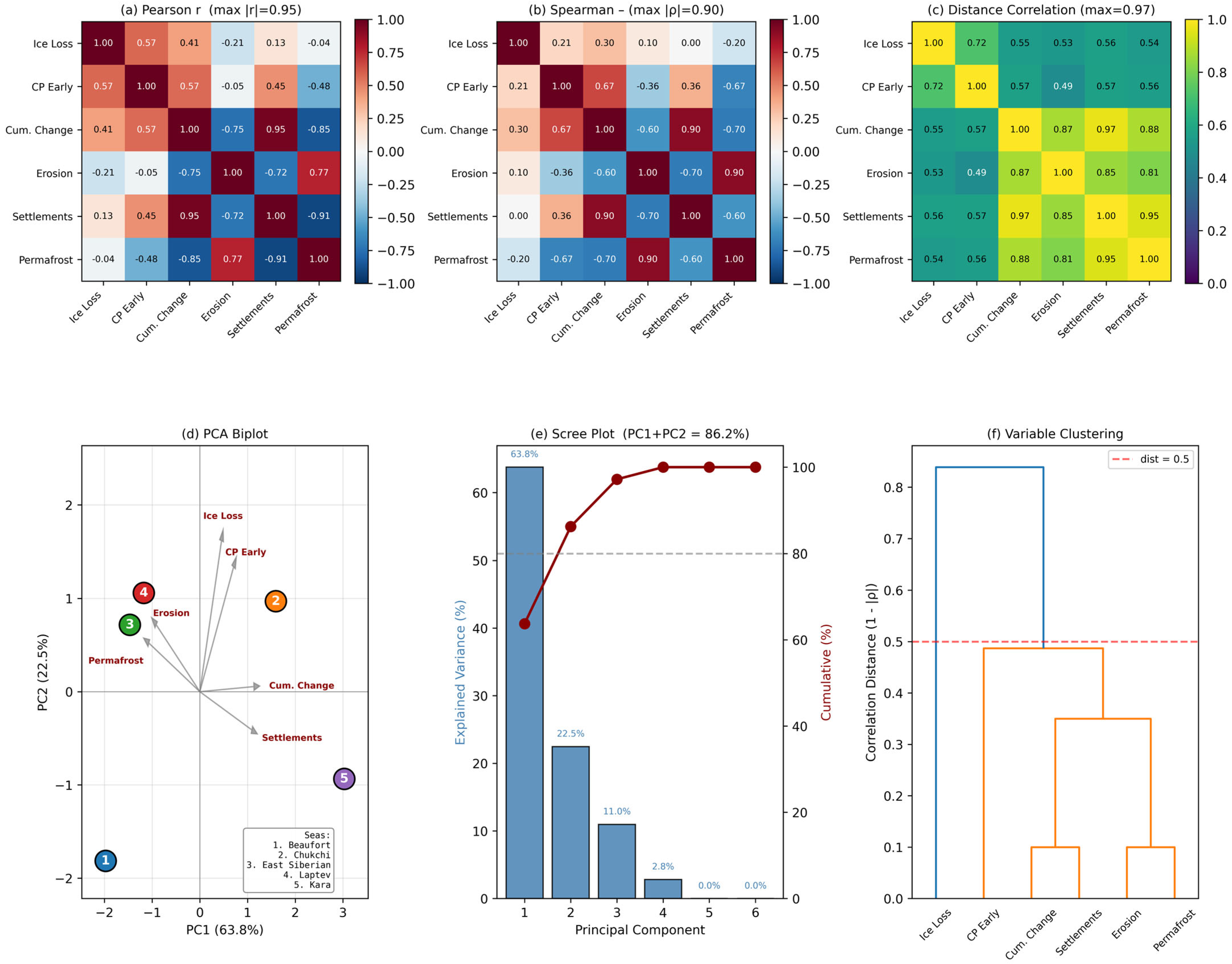
Figure A2.
Principal component analysis (PCA) re-weighting of the Composite Vulnerability Index. (a) Expert (baseline) weights for the six indicators; (b) PC1-loading–derived weights; (c) variance-weighted multi-PC (PCA-multi) weights; (d) CVI values for the five core seas under the baseline, PCA1-loading, and PCA-multi weighting schemes; (e) Spearman rank correlation of each PCA-weighted ranking with the baseline ranking (both ≥ the ρ = 0.80 threshold, shown as a dashed line); (f) rank agreement matrix showing the vulnerability rank (1 = most vulnerable) of each core sea under the three weighting schemes, confirming that all five ranks are preserved (PCA1-loading 5/5, PCA-multi 5/5), with the top-two seas (Chukchi, East Siberian) stable across all scenarios.
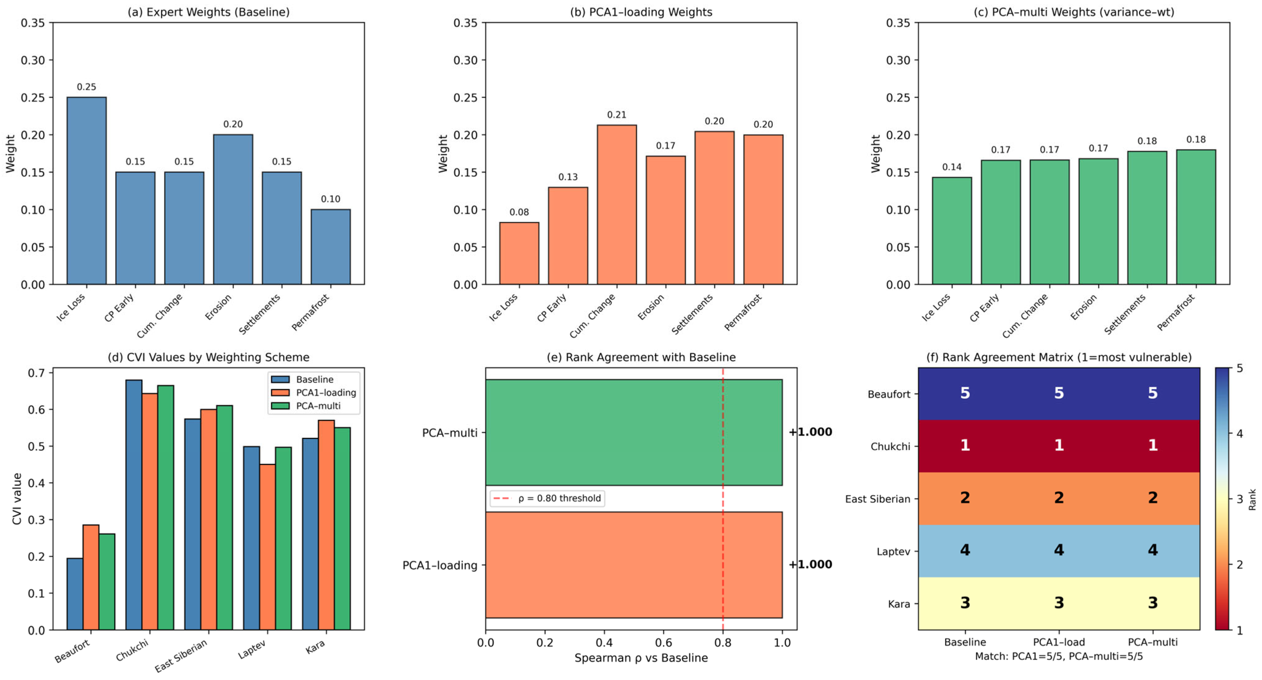
Figure A3.
One-at-a-time (OAT) and Monte Carlo sensitivity analysis of CVI weights. Each of the six indicator weights is perturbed by ±10%, ±25%, and ±50% from its baseline value (ice loss 0.25, CP early 0.15, cumulative change 0.15, erosion 0.20, settlements 0.15, permafrost 0.10) with the remaining weights renormalized. (a) Tornado plot of the resulting CVI score range per indicator (mean CVI standard deviation across the 0–3× multiplier range); (b) Monte Carlo CVI score distributions per core sea (uniform Dirichlet sampling, n = 300,000; yellow diamonds mark the baseline CVI); (c) rank stability heatmap showing the probability of each core sea occupying ranks 1–5 under MC uniform sampling; (d) full OAT curve of CVI versus the ice-loss weight multiplier (0–3×) for the five core seas, with the baseline multiplier (1×) marked; (e) CVI values for the five core seas under seven literature-based weighting scenarios (S1 baseline, S2 equal, S3 cryo-heavy, S4 exposure-heavy, S5 erosion focus, S6 settlement focus, S7 climate proxy); (f) Spearman rank correlation matrix between the seven weighting scenarios; (g) distribution of Spearman ρ versus the baseline CVI for bootstrap and Monte Carlo (uniform Dirichlet and base-centred) resampling, relative to the ρ = 0.80 robustness threshold; (h) top-rank probabilities P(rank = 1), P(top-2), and P(top-3) per core sea under MC uniform sampling; (i) baseline CVI versus the MC median with 95% confidence intervals per core sea. No single weight perturbation within ±50% alters the top-two ranking (Chukchi, East Siberian).
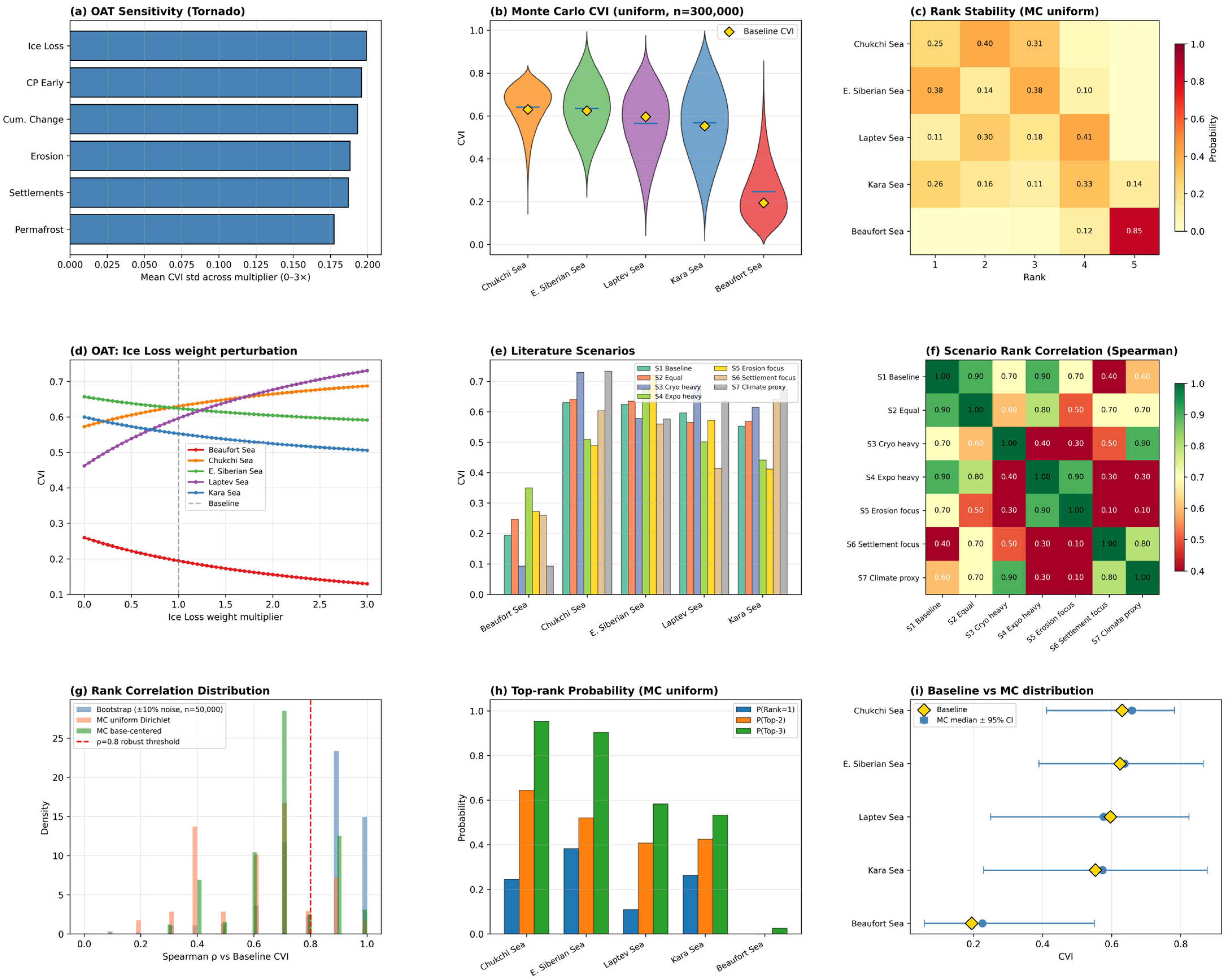
Figure A4.
Global sensitivity and Monte Carlo robustness analysis of the CVI. (a) Sobol’ first-order (S1) and total-order (St) sensitivity indices per indicator, averaged across the five core seas (error bars span the inter-sea range); (b) PAWN distribution-based sensitivity (median KS statistic) per indicator and sea; (c) top-k set stability across six Monte Carlo (MC) sampling scenarios, showing P(top-2) and P(top-3) identical to the baseline relative to the 10% random expectation; (d) consensus ranking of the five core seas under the baseline, Borda, and Copeland aggregation methods; (e) stress test showing each sea’s rank when a single indicator dominates (70% weight); (f) distribution of Spearman ρ versus the baseline CVI across all six MC scenarios, relative to the ρ = 0.80 robustness threshold; (g) the eight most frequent full ranking regimes under uniform MC sampling, with their probabilities (B = Beaufort, C = Chukchi, E = East Siberian, L = Laptev, K = Kara); (h) rank probability matrix giving the probability of each core sea occupying ranks 1–5 under uniform MC sampling; cells with a probability ≤ 0.02 are left blank for clarity; (i) probability that the Beaufort Sea is ranked lowest across all six MC scenarios, relative to the 20% random expectation. Across all diagnostics the top-two ranking (Chukchi, East Siberian) is preserved and Beaufort consistently ranks lowest.
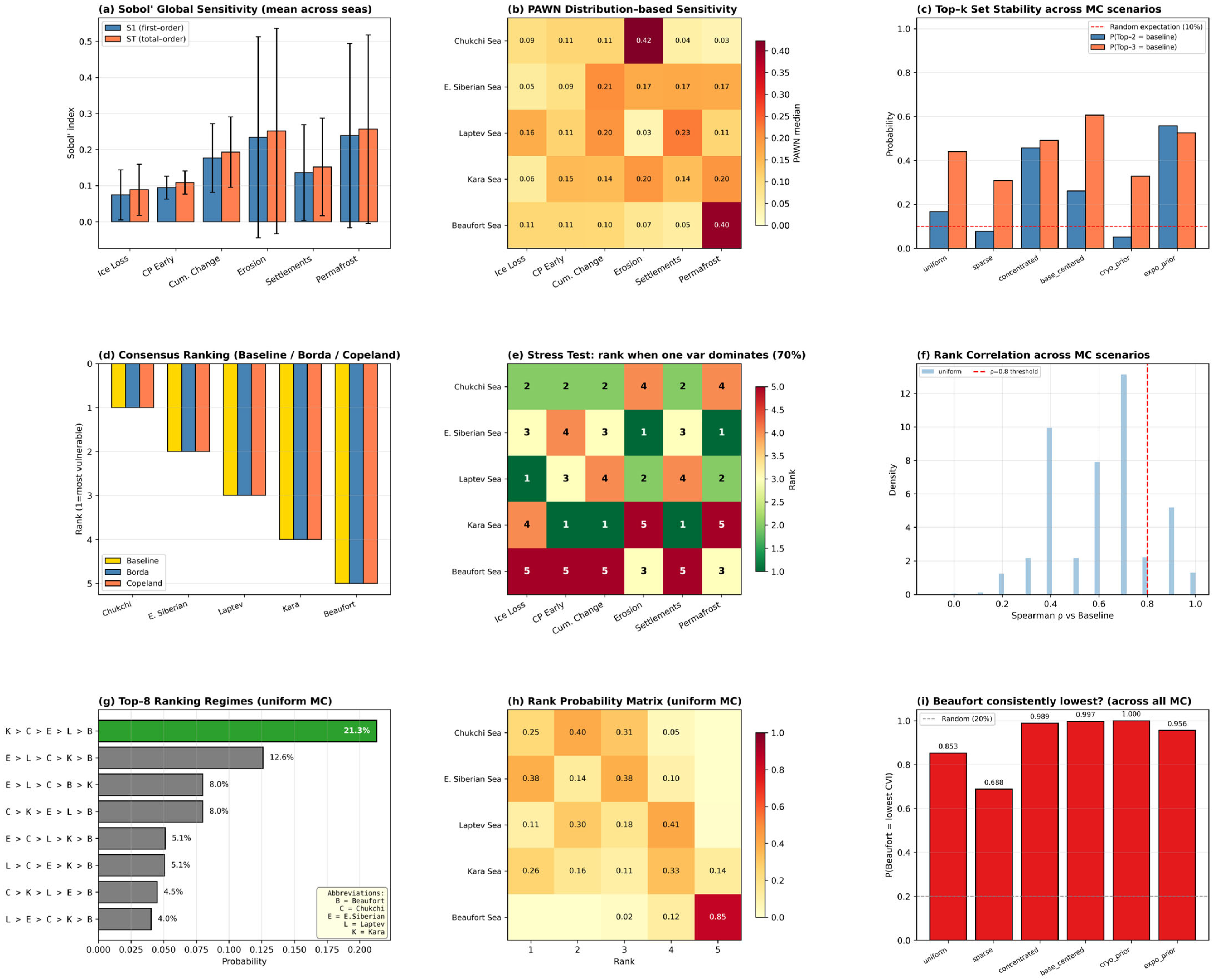
Figure A5.
CVI rank stability across alternative weighting scenarios. Yellow diamonds show the paper baseline CVI rank of each core sea (1 = highest vulnerability); blue markers and horizontal bars show the mean rank and the full rank range across the eight policy weighting scenarios. The top-two seas (Chukchi, East Siberian) remain in ranks 1–2 and the Beaufort Sea consistently occupies the lowest rank across all scenarios.
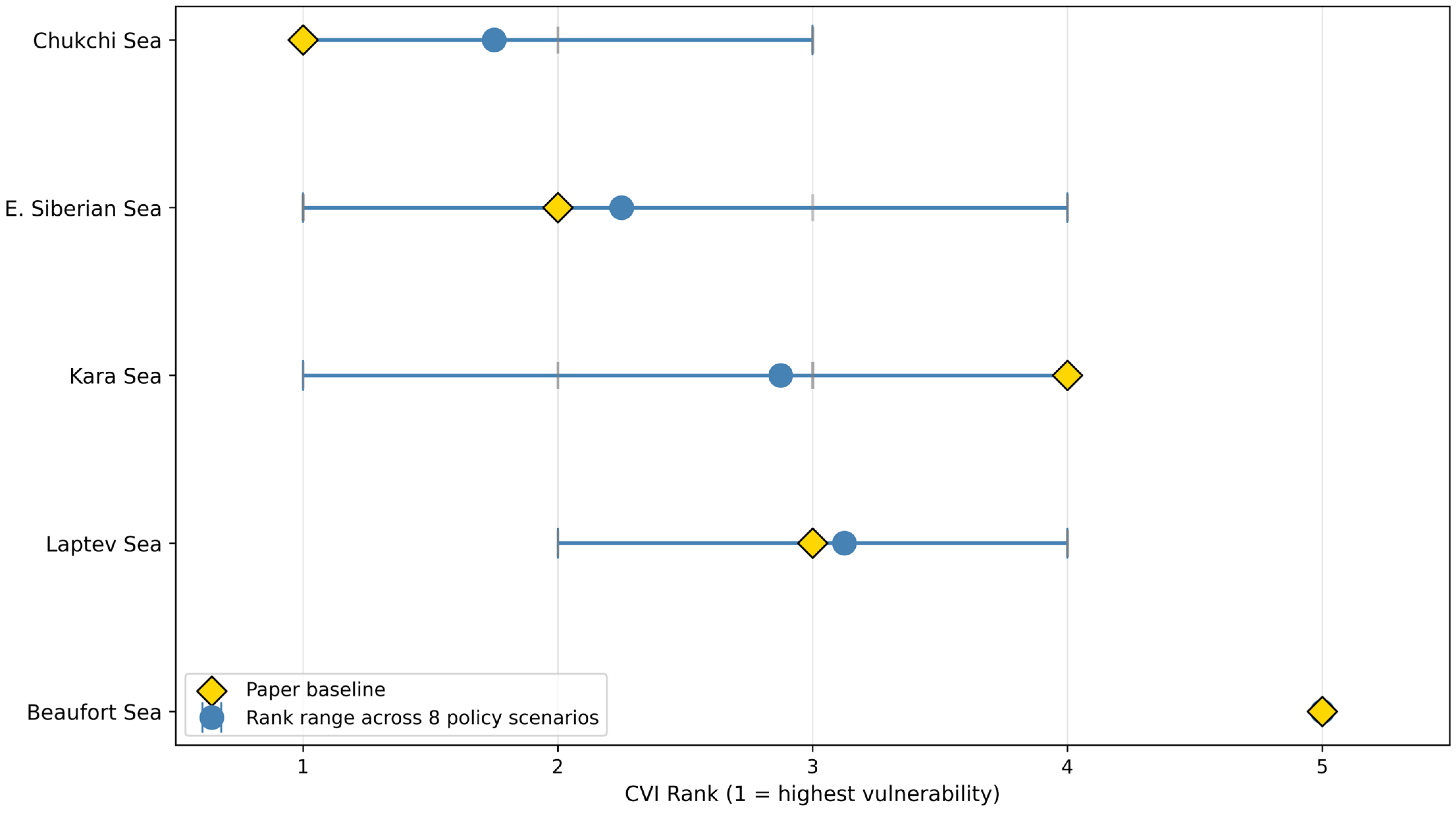
Figure A6.
Diagnostics for the weak basin-scale correlation between summer ice loss and coastal erosion rate across the five core seas (n = 5). (a) Scatter of coastal erosion rate versus summer ice loss, with the overall linear fit (Pearson r = −0.213 on the raw slope; r = 0.11 on the normalised CVI indicator cited in the main text; p = 0.73; 95% bootstrap CI shaded) and separate Atlantic-sector (n = 2) and Pacific-sector (n = 3) fits; (b) statistical power curve showing the minimum |r| detectable at α = 0.05 as a function of sample size—the observed r = 0.111 lies in the undetectable region at n = 5 and would require n ≥ 313 to be detected; (c) partial correlation and sector-stratified analysis of the ice-loss–erosion correlation, controlling individually for shelf depth, latitude, permafrost fraction, and Atlantic index, and split by Pacific and Atlantic sectors, relative to the ±0.88 significance threshold for n = 5; (d) forest plot of all effect sizes (raw Pearson, Spearman, Kendall, distance correlation, and partial correlations) with 95% bootstrap confidence intervals, with the undetectable region (n = 5) shaded. The weak basin mean correlation reflects limited statistical leverage and geographic confounding rather than the absence of physical coupling.
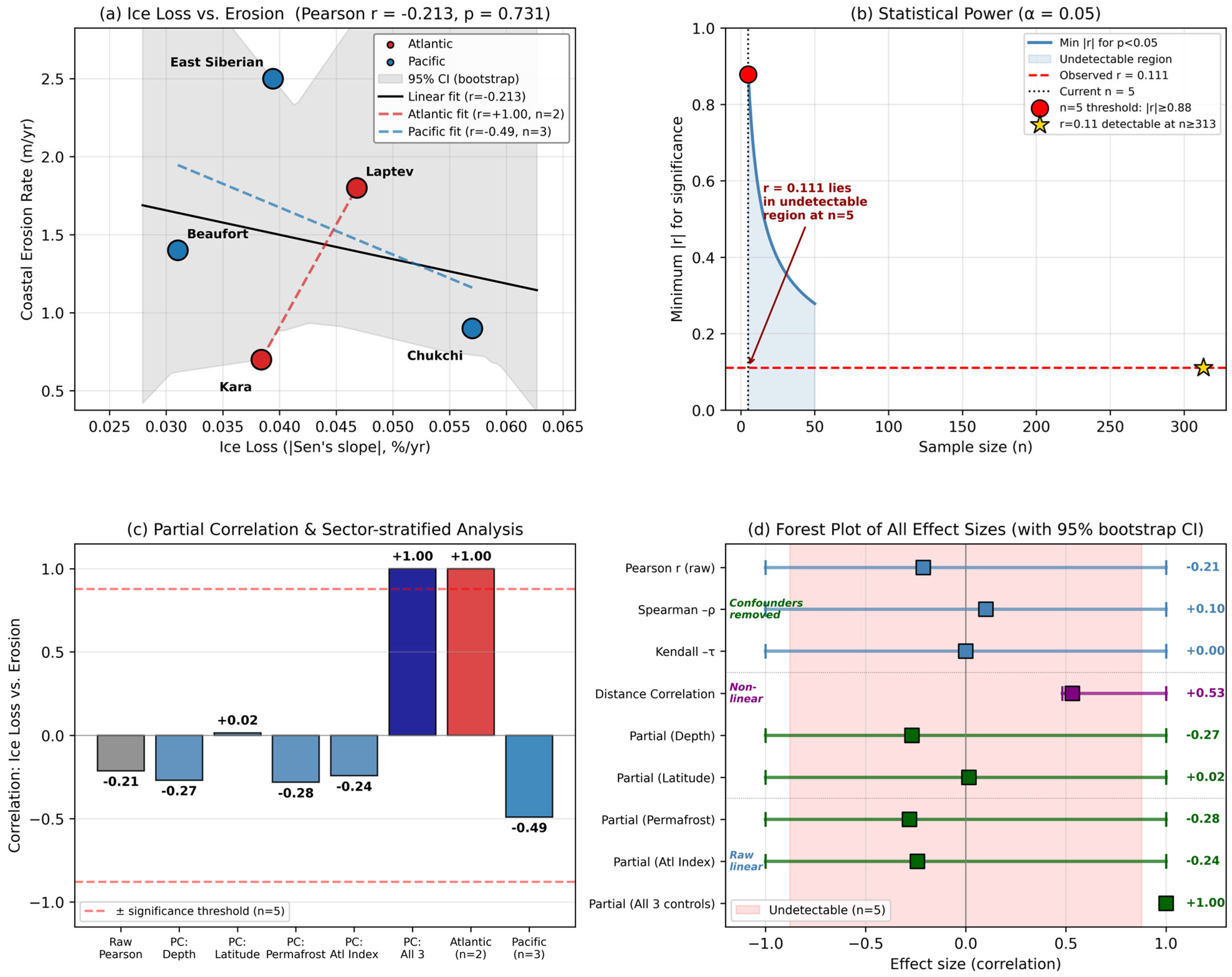
Figure A7.
Physical drivers and regime-shift timing across the nine pan-Arctic seas (S1–S9). Left: column-wise z-score heatmap of five physical drivers—latitude (°N), mean depth (m), shelf ratio (fraction of basin area shallower than 200 m), Atlantification index, and 1850s sea ice concentration (%); the raw value is annotated in each cell and the cell colour encodes the column-wise z-score (red = high, blue = low). Right: Pettitt change-point year for each sea (horizontal bars, annotated), with vertical dashed lines marking the core-sea mean (1936) and support-sea mean (≈1978). Red and blue side bars indicate core (permafrost-adjacent) and support seas, respectively. Data: SIBT1850 v2.0, GEBCO 2024 bathymetry [56], and the basin classification of Table 1.
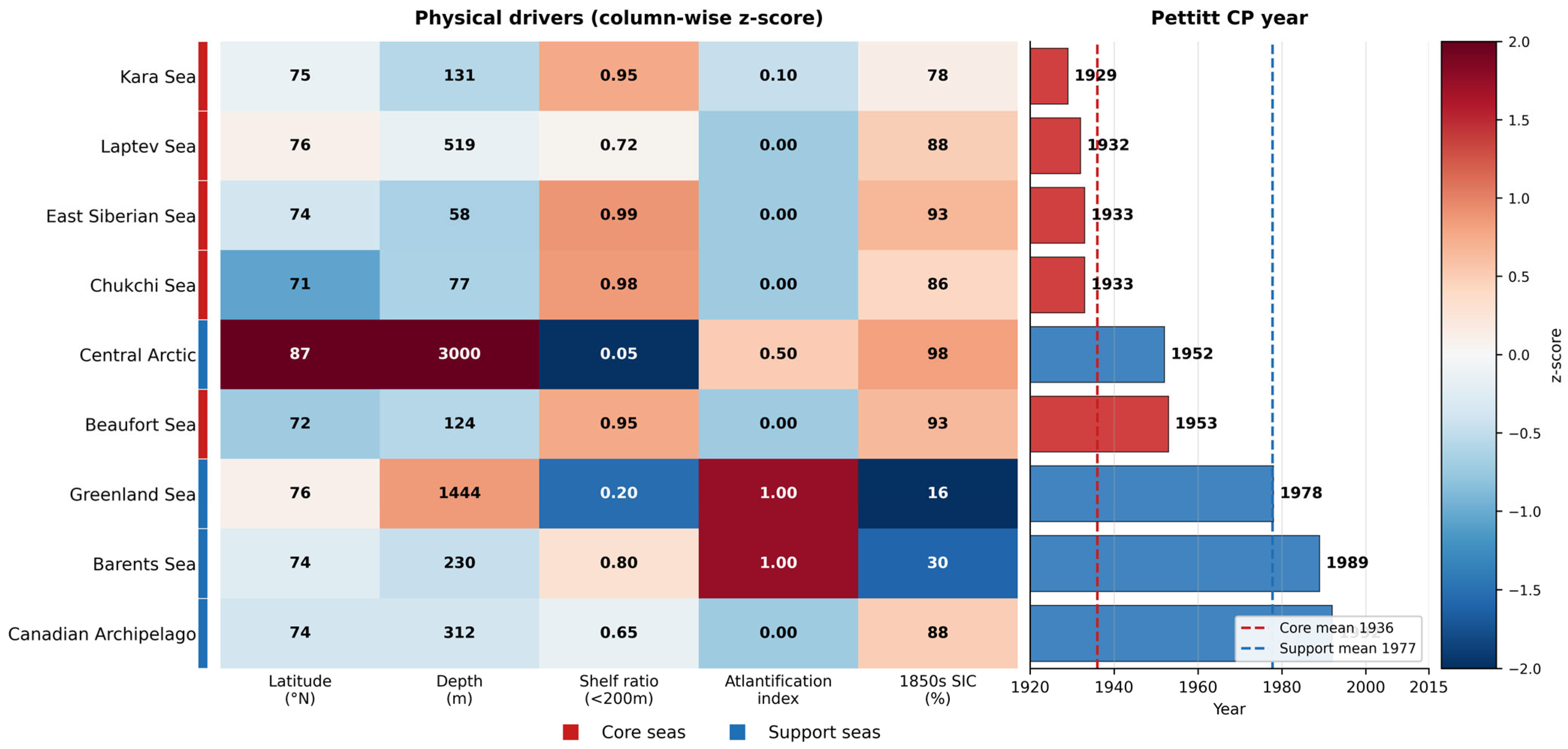
Table A1.
Indicator independence diagnostics. Multicollinearity diagnostics for the six CVI indicators across the five core seas (n = 5). VIF = variance inflation factor (capped at 104); max |r| values are taken from the off-diagonal of the Pearson, Spearman, and distance correlation (dCor) matrices. High VIF and max |r| > 0.9 motivate the PCA re-weighting (Table A4) and the alternative weighting robustness tests (Table A7 and Table A8).
Table A2.
Pearson correlation matrix (CVI indicators). Pearson linear correlation coefficients between the six CVI indicators across the five core seas. The strongest positive pair is ΔS–ST (r = 0.955); the strongest negative pair is ST–PF (r = −0.908). Compare with Table A3 (distance correlation) for non-linear dependence.
Table A3.
Distance correlation matrix (non-linear dependence). Distance correlation (dCor) between CVI indicators, which captures both linear and non-linear monotonic and non-monotonic dependence. All pairs exceed dCor = 0.48, confirming that the apparent low Pearson values (e.g., IL–ER, r = 0.111) hide substantial non-linear association.
Table A4.
PCA loadings and derived weights. Principal component analysis of the six CVI indicators across five core seas. PC1 (62.1%) and PC2 (28.2%) jointly explain 90.3% of variance; only PC1–PC2 are retained (Kaiser criterion). The right block lists three PCA-derived weighting schemes used in Table A5: W_PC1 = absolute PC1 loadings (normalised); W_PCA-multi = variance-weighted combination of PC1–PC2 absolute loadings; W_base = paper baseline for reference.
Table A5.
Baseline vs. PCA-weighted CVI rankings. Comparison of CVI scores and ranks across four weighting schemes: baseline (paper), PC1 loading weights, multi-PC weights, and pure PC1 scores. Top-2 seas (CHK, ESS) are preserved in three of four schemes; baseline–PCA-multi Spearman rank correlation ρ = 0.80.
Table A6.
Sobol Global Sensitivity Indices. Variance-based global sensitivity of CVI scores to the six weight inputs, by sea. S1 = first-order index (direct contribution); St = total-order index (including interactions); St − S1 < 0.10 throughout indicates weak interaction effects. Computed from 10,000 quasi-Monte-Carlo samples; 95% confidence intervals are within ±0.02 for all values.
Table A7.
CVI under alternative weighting scenarios. S1 = baseline (paper); S2 = equal weights (1/6 each); S3 = cryo-heavy (IL + CPE + ΔS + PF = 0.80); S4 = exposure-heavy (ER + ST = 0.70); S5 = erosion focus (ER = 0.50); S6 = settlement focus (ST = 0.50); S7 = climate attribution proxy (IL + CPE = 0.60). The top-2 set {CHK, ESS} is preserved in 5 of 7 scenarios; BFT is consistently ranked last (7/7).
Table A8.
Monte Carlo top-K rank stability. Dirichlet Monte Carlo weight perturbation results under six sampling regimes. n = number of weight vectors drawn; P_top2/P_top3 = probability that the simulated top-2/top-3 set is identical to the baseline; Jaccard = mean Jaccard similarity of top-K sets to baseline; lift = ratio of observed to random chance probability.
Table A9.
Diagnostics for the IL–ER correlation (r = 0.111). Bivariate, rank-based, non-linear, and partial correlation diagnostics for the basin-scale association between summer ice loss (IL) and coastal erosion rate (ER) across the five core seas (n = 5).
Table A10.
Mediation analysis: IL → PF → ER. Standardised path coefficients for a single-mediator model with summer ice loss (IL) as the exposure (X), permafrost fraction (PF) as the mediator (M), and erosion rate (ER) as the outcome (Y). Total effect c = 0.111 decomposes into a direct effect c′ = −0.180 and an indirect effect a × b = −0.033 (15.4% of total mediated through PF). The 95% bootstrap CI for the indirect effect spans zero, so the mediation is not statistically significant at n = 5.
Table A11.
Bimodal regime shift hypothesis tests. Three complementary tests of the hypothesis that Pettitt change point years differ between core (n = 5, mean 1936) and support seas (n = 4, mean ≈ 1978). The permutation test was repeated excluding the Central Arctic (deep-basin outlier with CP = 1952) and remains significant (Δ = 50.3 yr, p = 0.019).
Appendix B. Satellite-Era Robustness Check Using NSIDC G02202 v6 (1850–2024)
SIBT1850 is published as a fixed multi-centennial reconstruction terminating in 2017 and is not extended further by its producers; the 168-year backbone of the main text analysis therefore cannot itself be advanced to 2024 without losing the homogeneous reconstruction methodology that underpins it. To directly address concerns regarding the temporal currency of the analysis, we additionally extend the satellite-era portion of the record to 2024 using the NOAA/NSIDC Climate Data Record of Passive Microwave Sea Ice Concentration v6 (G02202 v6) [21]. The NSIDC 25 km Polar Stereographic grid (EPSG:3411) was projected onto the SIBT1850 0.25° lat/lon mesh through nearest-neighbour assignment, and the same area-weighted basin averaging was applied to obtain monthly and annual SIC time series for the nine regional seas. The combined SIBT1850 (1850–2017) + NSIDC v6 (2018–2024) record is used to repeat the trend, change point, and CVI analyses presented in Section 3.2, Section 3.3, Section 3.4, Section 3.5, Section 3.6 and Section 3.7.
Appendix B.1. Cross-Validation over the 1979–2017 Overlap
Over the 1979–2017 overlap period, annual mean SIBT1850 and NSIDC v6 agree to Pearson r ≥ 0.990 in all five core seas (Beaufort r = 0.996, Chukchi 0.996, East Siberian 0.996, Laptev 0.990, Kara 0.995), with mean biases between −0.32 and −1.01 SIC% and annual RMSEs ≤ 1.4 SIC%; support sea agreement is similarly high (r ≥ 0.978, bias −0.14 to −2.84 SIC%, RMSE ≤ 2.9 SIC%). The slightly larger NSIDC low biases in the marginal ice zone support seas (Greenland, Baffin/Gulf of St. Lawrence, Canadian Archipelago) are consistent with the well-documented tendency of the NASA Team/bootstrap algorithms underlying the G02202 v6 CDR to under-detect low-concentration ice in mixed surfaces and do not materially affect basin mean trend reconstruction. These overlap statistics justify treating the NSIDC v6 2018–2024 segment as a homogeneous satellite-era extension of the SIBT1850 record.
Figure A8.
SIBT1850 vs. NSIDC G02202 v6—annual mean SIC, 1979–2017, for the nine regional seas (S1–S9). Per-panel annotations report the annual mean Pearson r and mean bias (NSIDC − SIBT, pp). Five core seas exceed r = 0.99 and |bias| ≤ 1.0 pp.
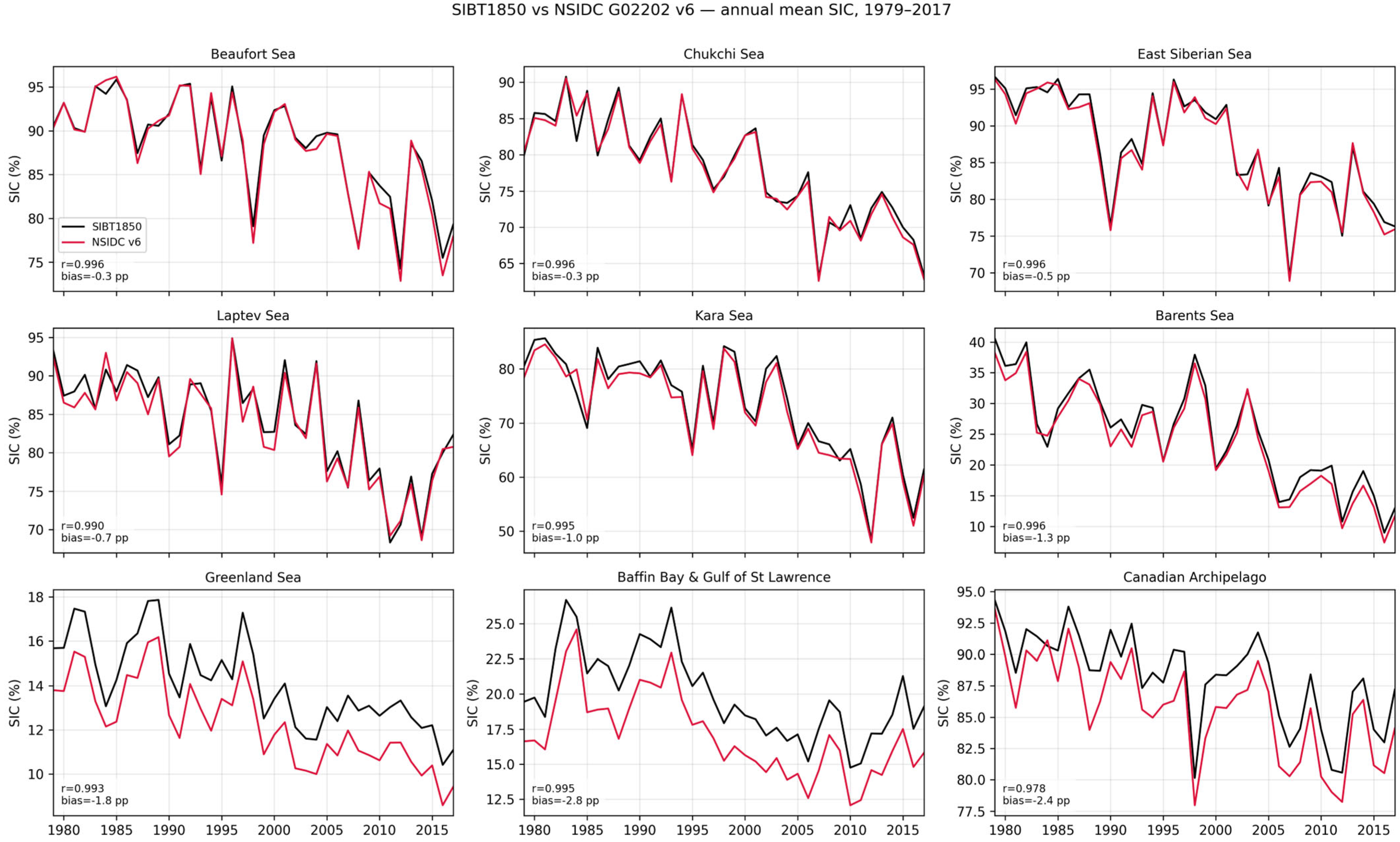
Appendix B.2. Extended Trend and Change Point Analysis (1850–2024)
Mann–Kendall trend, Sen’s slope, and Pettitt change point statistics were recomputed on the combined 175-year record (Table A12). All five core sea Pettitt change points remain within the 1929–1953 window of the SIBT1850-based analysis (Beaufort 1953 → 1953, Chukchi 1933 → 1942, East Siberian 1933 → 1933, Laptev 1932→1932, Kara 1929 → 1929). Annual Sen’s slopes retain sign and rank order while steepening by 10–25% under the extension (Chukchi −0.057 → −0.065%/yr; Laptev −0.047 → −0.058%/yr; East Siberian −0.039 → −0.050%/yr; Kara −0.038 → −0.053%/yr; Beaufort −0.031 → −0.039%/yr), consistent with continued post-2017 ice loss. Cumulative losses Δ (1850s decadal mean minus the 2015–2024 decadal mean) increase by 1.4–3.8 pp relative to the SIBT1850-only Δ (1850s → 2008–2017). A “bias-corrected” extension that removes the per-sea 1979–2017 mean bias from the 2018–2024 NSIDC segment differs from the raw extension by ≤0.1 pp in every reported quantity, confirming that the conclusions are insensitive to the small NSIDC–SIBT offset documented in Appendix B.1.
Figure A9.
Extended sea ice time series 1850–2024 for the nine regional seas (S1–S9). Black line: SIBT1850 annual mean (1850–2017); red line: NSIDC G02202 v6 annual mean (2018–2024). Dashed vertical lines mark Pettitt change point years recomputed on the combined record; for the four core seas in which the change point coincides with the SIBT1850 baseline this line is identical to that in Figure 3.
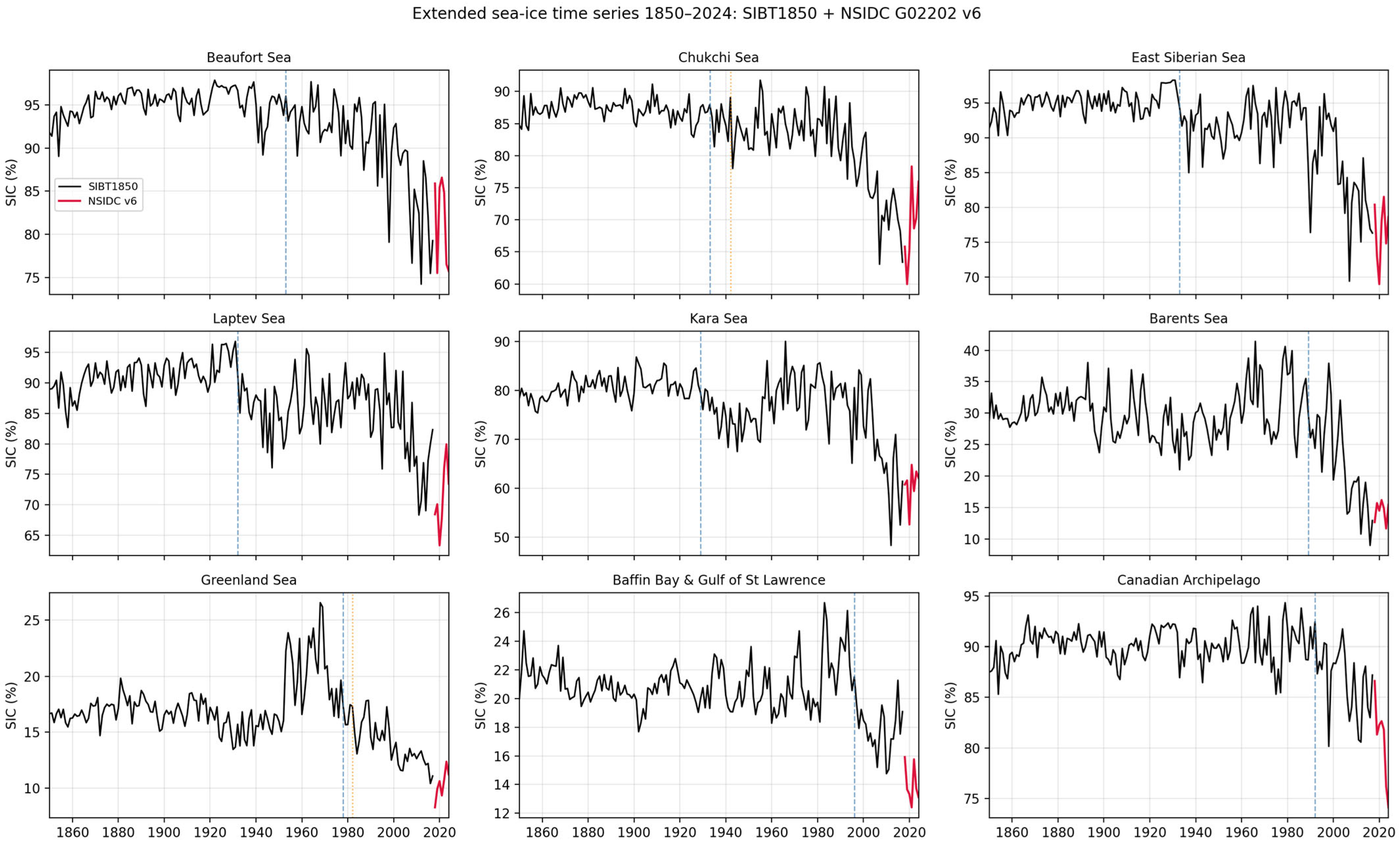
Appendix B.3. Extended CVI
The CVI was recomputed using the cryosphere indicators (IL, CPE, ΔS) derived from the combined 1850–2024 record while holding the static ER, ST, and PF indicators at their baseline values. The Chukchi–East Siberian–Laptev corridor is preserved as the top three highest-vulnerability basins; the Beaufort Sea retains rank 5; and the Spearman rank correlation between the baseline and extended CVI is ρ = 0.70 (Figure A10, Table A12). Within the top corridor the extended ranking promotes the East Siberian Sea to rank 1 (CVI 0.624 → 0.717) and the Laptev Sea to rank 2 (0.596 → 0.645), while the Chukchi Sea moves to rank 3 (0.630 → 0.558)—a reordering that reflects the steeper post-2017 summer loss of the East Siberian and Laptev seas and that strengthens, rather than weakens, the identification of the Chukchi–East Siberian–Laptev corridor as the pan-Arctic permafrost coastal vulnerability hotspot. We retain the SIBT1850-based ranking as the primary result for consistency with the 168-year backbone, while reporting the extended ranking here as a satellite-era robustness check.
Figure A10.
Composite Vulnerability Index: SIBT1850 baseline (1850–2017) vs. SIBT1850 + NSIDC v6 extended (1850–2024). (a) Bar plot of CVI scores per core sea under the two records; (b) rank shift diagram (slope chart) between baseline and extended ranks, with Spearman ρ between the two rankings.
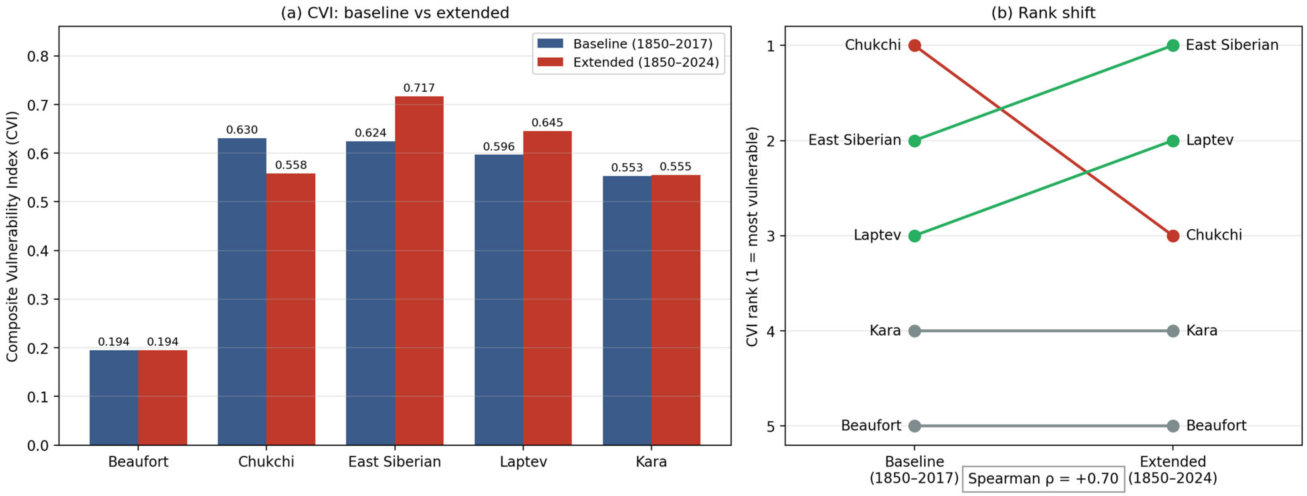
Table A12.
(a). Satellite-era cross-validation statistics (1979–2017). (b). Long-term trends and CVI: baseline (1850–2017) vs. extended (1850–2024). Sen_ann = annual Sen’s slope (%/yr); Pettitt = change point year; Δ = cumulative SIC change in pp (1850s → 2008–2017 for baseline, 1850s → 2015–2024 for extension). CVI is defined only over the five core seas (S1–S5); support seas and Baffin Bay & GoSL are shown with “—”.
Taken together, Figure A8, Figure A9 and Figure A10 and Table A12 demonstrate that (i) SIBT1850 and NSIDC G02202 v6 agree to better than 1 pp annual bias and r ≥ 0.99 across the five core seas over their 1979–2017 overlap, (ii) all five core sea Pettitt change points remain within the 1929–1953 window under the 1850–2024 extension, (iii) annual Sen’s slopes retain sign and rank order while steepening by 10–25%, consistent with continued post-2017 ice loss, and (iv) the CVI re-evaluation preserves the Chukchi–East Siberian–Laptev corridor as the top-three highest-vulnerability basins and retains Beaufort at rank 5. The qualitative identification of the Chukchi–East Siberian corridor as the pan-Arctic permafrost coastal vulnerability hotspot is therefore robust to inclusion of the most recent eight years of satellite observation.
References
- Rantanen, M.; Karpechko, A.; Lipponen, A.; Nordling, K.; Hyvärinen, O.; Ruosteenoja, K.; Vihma, T.; Laaksonen, A. The Arctic has warmed nearly four times faster than the globe since 1979. Commun. Earth Environ. 2022, 3, 168. [Google Scholar] [CrossRef] [Scilit]
- England, M.R.; Eisenman, I.; Lutsko, N.J.; Wagner, T.J.W. The Recent Emergence of Arctic Amplification. Geophys. Res. Lett. 2021, 48, e2021GL094086. [Google Scholar] [CrossRef] [Scilit]
- Sweeney, A.; Fu, Q.; Po-Chedley, S.; Wang, H.; Wang, M. Internal Variability Increased Arctic Amplification During 1980–2022. Geophys. Res. Lett. 2023, 50, e2023GL106060. [Google Scholar] [CrossRef] [Scilit]
- Zhou, W.; Leung, L.; Lu, J.; Rantanen, M.; England, M.; Serreze, M. Steady threefold Arctic amplification of externally forced warming masked by natural variability. Nat. Geosci. 2024, 17, 508–515. [Google Scholar] [CrossRef] [Scilit]
- Davy, R.; Griewank, P. Arctic amplification has already peaked. Environ. Res. Lett. 2023, 18, 094001. [Google Scholar] [CrossRef] [Scilit]
- Kumar, A.; Yadav, J.; Mohan, R. Global warming leading to alarming recession of the Arctic sea-ice cover: Insights from remote sensing observations and model reanalysis. Heliyon 2020, 6, e04355. [Google Scholar] [CrossRef] [Scilit] [PubMed]
- Meier, W.F. Losing Arctic Sea Ice: Observations of the Recent Decline and the Natural Long-Term Context. In Sea Ice, 3rd ed.; Thomas, D.N., Ed.; Wiley-Blackwell: Chichester, UK, 2017; pp. 290–303. [Google Scholar] [CrossRef] [Scilit]
- Walsh, J.; Fetterer, F.; Stewart, S.; Chapman, W. A database for depicting Arctic sea ice variations back to 1850. Geogr. Rev. 2017, 107, 89–107. [Google Scholar] [CrossRef] [Scilit]
- You, Q.; Cai, Z.; Pepin, N.; Chen, D.; Ahrens, B.; Jiang, Z.; Wu, F.; Kang, S.; Zhang, R.; Wu, T.; et al. Warming amplification over the Arctic Pole and Third Pole: Trends, mechanisms and consequences. Earth-Sci. Rev. 2021, 216, 103625. [Google Scholar] [CrossRef] [Scilit]
- Comiso, J.; Parkinson, C.; Gersten, R.; Stock, L. Accelerated decline in the Arctic sea ice cover. Geophys. Res. Lett. 2008, 35, L01703. [Google Scholar] [CrossRef] [Scilit]
- Serreze, M.; Meier, W. The Arctic’s sea ice cover: Trends, variability, predictability, and comparisons to the Antarctic. Ann. N. Y. Acad. Sci. 2018, 1436, 5–20. [Google Scholar] [CrossRef] [Scilit] [PubMed]
- Meier, W.; Stroeve, J.; Fetterer, F. Whither Arctic sea ice? A clear signal of decline regionally, seasonally and extending beyond the satellite record. Ann. Glaciol. 2007, 46, 428–434. [Google Scholar] [CrossRef] [Scilit]
- Box, J.; Colgan, W.; Christensen, T.; Schmidt, N.; Lund, M.; Parmentier, F.; Brown, R.; Bhatt, U.; Euskirchen, E.; Romanovsky, V.; et al. Key indicators of Arctic climate change: 1971–2017. Environ. Res. Lett. 2019, 14, 045010. [Google Scholar] [CrossRef] [Scilit]
- Bai, Y.; Sicre, M.; Ren, J.; Jalali, B.; Klein, V.; Li, H.; Lin, L.; Ji, Z.; Su, L.; Zhu, Q.; et al. Centennial-scale variability of sea-ice cover in the Chukchi Sea since AD 1850 based on biomarker reconstruction. Environ. Res. Lett. 2022, 17, 044058. [Google Scholar] [CrossRef] [Scilit]
- Brennan, M.; Hakim, G.; Blanchard-Wrigglesworth, E. Arctic Sea-Ice Variability During the Instrumental Era. Geophys. Res. Lett. 2020, 47, e2019GL086843. [Google Scholar] [CrossRef] [Scilit]
- Pirón, M.J.; Pasalodos, J.A.C. Nueva serie de extensión del hielo marino ártico en septiembre entre 1935 y 2014. Rev. De Climatol. 2016, 16, 1–19. [Google Scholar] [CrossRef] [Scilit]
- Kinnard, C.; Zdanowicz, C.; Fisher, D.; Isaksson, E.; Vernal, A.; Thompson, L. Reconstructed changes in Arctic sea ice over the past 1450 years. Nature 2011, 479, 509–512. [Google Scholar] [CrossRef] [Scilit] [PubMed]
- Leclerc, N.; Halfar, J. Review of Arctic sea-ice records over the last millennium from modern, historical and proxy data sources. Arct. Antarct. Alp. Res. 2024, 56, 2394894. [Google Scholar] [CrossRef] [Scilit]
- Wang, R.; Li, S.; Zhe, H. Evaluation of the HadISST1 and NSIDC 1850 onward sea ice datasets with a focus on the Barents-Kara seas. Atmos. Ocean. Sci. Lett. 2018, 11, 388–395. [Google Scholar] [CrossRef] [Scilit]
- Titchner, H.A.; Rayner, N.A. The Met Office Hadley Centre sea ice and sea surface temperature data set, version 2: 1. Sea ice concentrations. J. Geophys. Res. Atmos. 2014, 119, 2864–2889. [Google Scholar] [CrossRef] [Scilit]
- Meier, W.N.; Stewart, J.S.; DiGirolamo, N.E.; Hardman, M. NOAA/NSIDC Climate Data Record of Passive Microwave Sea Ice Concentration, Version 6 (G02202, v6 Enhancements); National Snow and Ice Data Center: Boulder, CO, USA, 2023. [Google Scholar] [CrossRef] [Scilit]
- Schweiger, A.; Wood, K.; Zhang, J. Arctic Sea Ice Volume Variability over 1901–2010: A Model-Based Reconstruction. J. Clim. 2019, 32, 4839–4849. [Google Scholar] [CrossRef] [Scilit]
- Overeem, I.; Anderson, R.; Wobus, C.; Clow, G.; Urban, F.; Matell, N. Sea ice loss enhances wave action at the Arctic coast. Geophys. Res. Lett. 2011, 38, L17503. [Google Scholar] [CrossRef] [Scilit]
- Nielsen, D.; Pieper, P.; Barkhordarian, A.; Overduin, P.; Ilyina, T.; Brovkin, V.; Baehr, J.; Dobrynin, M. Increase in Arctic coastal erosion and its sensitivity to warming in the twenty-first century. Nat. Clim. Change 2022, 12, 263–270. [Google Scholar] [CrossRef] [Scilit]
- Baranskaya, A.; Novikova, A.; Shabanova, N.; Belova, N.; Maznev, S.; Ogorodov, S.; Jones, B. The Role of Thermal Denudation in Erosion of Ice-Rich Permafrost Coasts in an Enclosed Bay (Gulf of Kruzenstern, Western Yamal, Russia). Front. Earth Sci. 2021, 8, 566227. [Google Scholar] [CrossRef] [Scilit]
- Creel, R.; Guimond, J.; Jones, B.; Nielsen, D.; Bristol, E.; Tweedie, C.; Overduin, P. Permafrost thaw subsidence, sea-level rise, and erosion are transforming Alaska’s Arctic coastal zone. Proc. Natl. Acad. Sci. USA 2024, 121, e2409411121. [Google Scholar] [CrossRef] [Scilit] [PubMed]
- Barnhart, K.; Anderson, R.; Overeem, I.; Wobus, C.; Clow, G.; Urban, F. Modeling erosion of ice-rich permafrost bluffs along the Alaskan Beaufort Sea coast. J. Geophys. Res. Earth Surf. 2014, 119, 1155–1179. [Google Scholar] [CrossRef] [Scilit]
- Nielsen, D.; Dobrynin, M.; Baehr, J.; Razumov, S.; Grigoriev, M. Coastal Erosion Variability at the Southern Laptev Sea Linked to Winter Sea Ice and the Arctic Oscillation. Geophys. Res. Lett. 2020, 47, e2019GL086876. [Google Scholar] [CrossRef] [Scilit]
- Günther, F.; Overduin, P.; Sandakov, A.; Grosse, G.; Grigoriev, M. Short- and long-term thermo-erosion of ice-rich permafrost coasts in the Laptev Sea region. Biogeosciences 2013, 10, 4297–4318. [Google Scholar] [CrossRef] [Scilit]
- Jones, B.; Farquharson, L.; Baughman, C.; Buzard, R.; Arp, C.; Grosse, G.; Bull, D.; Günther, F.; Nitze, I.; Urban, F.; et al. A decade of remotely sensed observations highlight complex processes linked to coastal permafrost bluff erosion in the Arctic. Environ. Res. Lett. 2018, 13, 094011. [Google Scholar] [CrossRef] [Scilit]
- Jones, M.; Jones, B.; Nitze, I.; Gessner, M.; Grosse, G.; Bartsch, A.; Bull, D. Annual and sub-seasonal dynamics of a rapidly eroding permafrost coastline along the Beaufort Sea in northern Alaska. Sci. Rep. 2025, 15, 6823. [Google Scholar] [CrossRef] [Scilit] [PubMed]
- Cunliffe, A.M.; Tanski, G.; Radosavljevic, B.; Palmer, W.F.; Sachs, T.; Lantuit, H.; Kerby, J.T.; Myers-Smith, I.H. Rapid retreat of permafrost coastline observed with aerial drone photogrammetry. Cryosphere 2019, 13, 1513–1528. [Google Scholar] [CrossRef] [Scilit]
- Radosavljevic, B.; Lantuit, H.; Pollard, W.; Overduin, P.; Couture, N.; Sachs, T.; Helm, V.; Fritz, M. Erosion and Flooding—Threats to Coastal Infrastructure in the Arctic: A Case Study from Herschel Island, Yukon Territory, Canada. Estuaries Coasts 2016, 39, 900–915. [Google Scholar] [CrossRef] [Scilit]
- Gibbs, A.; Erikson, L.; Jones, B.; Richmond, B.; Engelstad, A. Seven Decades of Coastal Change at Barter Island, Alaska: Exploring the Importance of Waves and Temperature on Erosion of Coastal Permafrost Bluffs. Remote Sens. 2021, 13, 4420. [Google Scholar] [CrossRef] [Scilit]
- Cassidy, G.; Wiseman, M.; Lange, K.; Eilers, C.; Bradley, A. Seasonal Coastal Erosion Rates Calculated from PlanetScope Imagery in Arctic Alaska. Remote Sens. 2024, 16, 2365. [Google Scholar] [CrossRef] [Scilit]
- Ramage, J.; Jungsberg, L.; Wang, S.; Westermann, S.; Lantuit, H.; Heleniak, T. Population living on permafrost in the Arctic. Popul. Environ. 2021, 43, 22–38. [Google Scholar] [CrossRef] [Scilit]
- Tanguy, R.; Bartsch, A.; Nitze, I.; Irrgang, A.; Petzold, P.; Widhalm, B.; Von Baeckmann, C.; Boike, J.; Martin, J.; Efimova, A.; et al. Pan-Arctic Assessment of Coastal Settlements and Infrastructure Vulnerable to Coastal Erosion, Sea-Level Rise, and Permafrost Thaw. Earth’s Future 2024, 12, e2024EF005013. [Google Scholar] [CrossRef] [Scilit]
- Bartsch, A.; Pointner, G.; Nitze, I.; Efimova, A.; Jakober, D.; Ley, S.; Högström, E.; Grosse, G.; Schweitzer, P. Expanding infrastructure and growing anthropogenic impacts along Arctic coasts. Environ. Res. Lett. 2021, 16, 115013. [Google Scholar] [CrossRef] [Scilit]
- Forbes, B.; Stammler, F.; Kumpula, T.; Meschtyb, N.; Pajunen, A.; Kaarlejärvi, E. High resilience in the Yamal-Nenets social–ecological system, West Siberian Arctic, Russia. Proc. Natl. Acad. Sci. USA 2009, 106, 22041–22048. [Google Scholar] [CrossRef] [Scilit] [PubMed]
- Bartsch, A.; Pointner, G.; Ingeman-Nielsen, T.; Lu, W. Towards Circumpolar Mapping of Arctic Settlements and Infrastructure Based on Sentinel-1 and Sentinel-2. Remote Sens. 2020, 12, 2368. [Google Scholar] [CrossRef] [Scilit]
- Ford, J.; Pearce, T.; Canosa, I.; Harper, S. The rapidly changing Arctic and its societal implications. Wiley Interdiscip. Rev. Clim. Change 2021, 12, e735. [Google Scholar] [CrossRef] [Scilit]
- Barnhart, K.; Overeem, I.; Anderson, R. The effect of changing sea ice on the physical vulnerability of Arctic coasts. Cryosphere 2014, 8, 1777–1799. [Google Scholar] [CrossRef] [Scilit]
- Henke, M.; Miesse, T.; De Lima, A.; Ferreira, C.; Ravens, T. Increasing coastal exposure to extreme wave events in the Alaskan Arctic as the open water season expands. Commun. Earth Environ. 2024, 5, 123. [Google Scholar] [CrossRef] [Scilit]
- Cai, Q.; Beletsky, D.; Wang, J.; Lei, R. Interannual and decadal variability of Arctic summer sea ice associated with atmospheric teleconnection patterns during 1850–2017. J. Clim. 2021, 34, 2921–2936. [Google Scholar] [CrossRef] [Scilit]
- Onarheim, I.; Eldevik, T.; Smedsrud, L.; Stroeve, J. Seasonal and Regional Manifestation of Arctic Sea Ice Loss. J. Clim. 2018, 31, 4917–4932. [Google Scholar] [CrossRef] [Scilit]
- Hirahara, S.; Ishii, M.; Fukuda, Y. Centennial-Scale Sea Surface Temperature Analysis and Its Uncertainty. J. Clim. 2014, 27, 57–75. [Google Scholar] [CrossRef] [Scilit]
- Parkinson, C. Arctic sea ice coverage from 43 years of satellite passive-microwave observations. Front. Remote Sens. 2022, 3, 1021781. [Google Scholar] [CrossRef] [Scilit]
- Ran, Y.; Li, X.; Cheng, G.; Che, J.; Aalto, J.; Karjalainen, O.; Hjort, J.; Luoto, M.; Jin, H.; Obu, J.; et al. New high-resolution estimates of the permafrost thermal state and hydrothermal conditions over the Northern Hemisphere. Earth Syst. Sci. Data 2022, 14, 865–884. [Google Scholar] [CrossRef] [Scilit]
- Obu, J.; Westermann, S.; Bartsch, A.; Berdnikov, N.; Christiansen, H.H.; Dashtseren, A.; Delaloye, R.; Elberling, B.; Etzelmüller, B.; Kholodov, A.; et al. Northern Hemisphere permafrost map based on TTOP modelling for 2000–2016 at 1 km2 scale. Earth-Sci. Rev. 2019, 193, 299–316. [Google Scholar] [CrossRef] [Scilit]
- Hetzinger, S.; Halfar, J.; Zajacz, Z.; Wisshak, M. Early start of 20th-century Arctic sea-ice decline recorded in Svalbard coralline algae. Geology 2019, 47, 307–310. [Google Scholar] [CrossRef] [Scilit]
- Ingrosso, G.; Ceccarelli, C.; Giglio, F.; Giordano, P.; Hefter, J.; Langone, L.; Miserocchi, S.; Mollenhauer, G.; Nogarotto, A.; Sabino, M.; et al. Greening of Svalbard in the twentieth century driven by sea ice loss and glaciers retreat. Commun. Earth Environ. 2025, 6, 123. [Google Scholar] [CrossRef] [Scilit]
- Dörr, J.; Årthun, M.; Eldevik, T.; Madonna, E. Mechanisms of regional winter sea-ice variability in a warming Arctic. J. Clim. 2021, 34, 8977–8995. [Google Scholar] [CrossRef] [Scilit]
- Wang, Q.; Danilov, S. A Synthesis of the Upper Arctic Ocean Circulation During 2000–2019: Understanding the Roles of Wind Forcing and Sea Ice Decline. Front. Mar. Sci. 2022, 9, 863204. [Google Scholar] [CrossRef] [Scilit]
- Novikova, A.; Belova, N.; Baranskaya, A.; Aleksyutina, D.; Maslakov, A.; Zelenin, E.; Shabanova, N.; Ogorodov, S. Dynamics of Permafrost Coasts of Baydaratskaya Bay (Kara Sea) Based on Multi-Temporal Remote Sensing Data. Remote Sens. 2018, 10, 1481. [Google Scholar] [CrossRef] [Scilit]
- Andersson, T.; Hosking, J.; Pérez-Ortiz, M.; Paige, B.; Elliott, A.; Russell, C.; Law, S.; Jones, D.; Wilkinson, J.; Phillips, T.; et al. Seasonal Arctic sea ice forecasting with probabilistic deep learning. Nat. Commun. 2021, 12, 5124. [Google Scholar] [CrossRef] [Scilit] [PubMed]
- GEBCO Bathymetric Compilation Group. The GEBCO_2024 Grid—A Continuous Terrain Model of the Global Oceans and Land. NERC EDS British Oceanographic Data Centre NOC. 2024. Available online: https://www.bodc.ac.uk/data/published_data_library/catalogue/10.5285/1c44ce99-0a0d-5f4f-e063-7086abc0ea0f/ (accessed on 2 June 2026).
- Sudarsan, G.; Lasitha, A. Rainfall Trend analysis using Mann-Kendall and Sen’s slope test estimation—A case study. In Proceedings of the 2023 International Conference on Sustainable Technologies in Civil and Environmental Engineering (ICSTCE 2023), Pune, India, 15–16 June 2023; Volume 405, p. 04013. [Google Scholar] [CrossRef] [Scilit]
- Garba, H.; Udokpoh, U. Analysis of Trend in Meteorological and Hydrological Time-series using Mann-Kendall and Sen’s Slope Estimator Statistical Test in Akwa Ibom State, Nigeria. Int. J. Environ. Clim. Change 2023, 13, 1029–1042. [Google Scholar] [CrossRef] [Scilit]
- Wang, F.; Shao, W.; Yu, H.; Kan, G.; He, X.; Zhang, D.; Ren, M.; Wang, G. Re-evaluation of the Power of the Mann-Kendall Test for Detecting Monotonic Trends in Hydrometeorological Time Series. Front. Earth Sci. 2020, 8, 14. [Google Scholar] [CrossRef] [Scilit]
- Liew, M.; Xiao, M.; Farquharson, L.; Nicolsky, D.; Jensen, A.; Romanovsky, V.; Peirce, J.; Alessa, L.; McComb, C.; Zhang, X.; et al. Understanding Effects of Permafrost Degradation and Coastal Erosion on Civil Infrastructure in Arctic Coastal Villages: A Community Survey and Knowledge Co-Production. J. Mar. Sci. Eng. 2022, 10, 422. [Google Scholar] [CrossRef] [Scilit]
- Philipp, M.; Dietz, A.; Ullmann, T.; Kuenzer, C. Automated Extraction of Annual Erosion Rates for Arctic Permafrost Coasts Using Sentinel-1, Deep Learning, and Change Vector Analysis. Remote Sens. 2022, 14, 3656. [Google Scholar] [CrossRef] [Scilit]
- Pastíriková, L.; Hrbáček, F.; Uxa, T.; Láska, K. Permafrost table temperature and active layer thickness variability on James Ross Island, Antarctic Peninsula, in 2004–2021. Sci. Total Environ. 2023, 869, 161690. [Google Scholar] [CrossRef] [Scilit] [PubMed]
- Tsai, Y. Monitoring Arctic permafrost coastal erosion dynamics using a multidecadal cross-mission SAR dataset along an Alaskan Beaufort Sea coastline. Sci. Total Environ. 2024, 912, 170389. [Google Scholar] [CrossRef] [Scilit] [PubMed]
- Ali, N.; Ghani, N.A. A Comparison of the Rank-based and Slope-based Nonparametric Tests for Trend Detection in Climate Time Series. Appl. Math. Comput. Intell. 2024, 13, 1–15. [Google Scholar] [CrossRef] [Scilit]
- Aswad, F.; Yousif, A.; Ibrahim, S. Trend Analysis Using Mann-Kendall and Sen’s Slope Estimator Test for Annual and Monthly Rainfall for Sinjar District, Iraq. J. Univ. Duhok 2020, 23, 41–54. [Google Scholar] [CrossRef] [Scilit]
- Kocsis, T.; Kovács-Székely, I.; Anda, A. Homogeneity tests and non-parametric analyses of tendencies in precipitation time series in Keszthely, Western Hungary. Theor. Appl. Climatol. 2019, 139, 849–859. [Google Scholar] [CrossRef] [Scilit]
- Mallakpour, I.; Villarini, G. A simulation study to examine the sensitivity of the Pettitt test to detect abrupt changes in mean. Hydrol. Sci. J. 2016, 61, 245–254. [Google Scholar] [CrossRef] [Scilit]
- Ryberg, K.; Hodgkins, G.; Dudley, R. Change points in annual peak streamflows: Method comparisons and historical change points in the United States. J. Hydrol. 2020, 583, 124307. [Google Scholar] [CrossRef] [Scilit]
- Conte, L.; Bayer, D.; Bayer, F. Bootstrap Pettitt test for detecting change points in hydroclimatological data: Case study of Itaipu Hydroelectric Plant, Brazil. Hydrol. Sci. J. 2019, 64, 1312–1326. [Google Scholar] [CrossRef] [Scilit]
- Kwok, R. Arctic sea ice thickness, volume, and multiyear ice coverage: Losses and coupled variability (1958–2018). Environ. Res. Lett. 2018, 13, 105005. [Google Scholar] [CrossRef] [Scilit]
- Sumata, H.; de Steur, L.; Divine, D.V.; Granskog, M.A.; Gerland, S. Regime shift in Arctic Ocean sea ice thickness. Nature 2023, 615, 443–449. [Google Scholar] [CrossRef] [Scilit] [PubMed]
- Fang, M.; Li, X.; Chen, H.; Chen, D. Arctic amplification modulated by Atlantic Multidecadal Oscillation and greenhouse forcing on multidecadal to century scales. Nat. Commun. 2022, 13, 1228. [Google Scholar] [CrossRef] [Scilit] [PubMed]
- Park, H.; Watanabe, E.; Kim, Y.; Polyakov, I.; Oshima, K.; Zhang, X.; Kimball, J.; Yang, D. Increasing riverine heat influx triggers Arctic sea ice decline and oceanic and atmospheric warming. Sci. Adv. 2020, 6, eabc4699. [Google Scholar] [CrossRef] [Scilit] [PubMed]
- Casas-Prat, M.; Wang, X. Projections of Extreme Ocean Waves in the Arctic and Potential Implications for Coastal Inundation and Erosion. J. Geophys. Res. Ocean. 2020, 125, e2019JC015745. [Google Scholar] [CrossRef] [Scilit]
- Mann, P.; Strauss, J.; Palmtag, J.; Dowdy, K.; Ogneva, O.; Fuchs, M.; Bedington, M.; Torres, R.; Polimene, L.; Overduin, P.; et al. Degrading permafrost river catchments and their impact on Arctic Ocean nearshore processes. Ambio 2021, 51, 439–455. [Google Scholar] [CrossRef] [Scilit] [PubMed]
- AMAP. Arctic Climate Change Update 2021: Key Trends and Impacts. Summary for Policy-Makers; Arctic Monitoring and Assessment Programme (AMAP): Tromsø, Norway, 2021; 16p. [Google Scholar]
- Tedesco, L.; Vichi, M.; Scoccimarro, E. Sea-ice algal phenology in a warmer Arctic. Sci. Adv. 2019, 5, eav4830. [Google Scholar] [CrossRef] [Scilit] [PubMed]
- Lannuzel, D.; Tedesco, L.; Van Leeuwe, M.; Campbell, K.; Flores, H.; Delille, B.; Miller, L.; Stefels, J.; Assmy, P.; Bowman, J.; et al. The future of Arctic sea-ice biogeochemistry and ice-associated ecosystems. Nat. Clim. Change 2020, 10, 983–992. [Google Scholar] [CrossRef] [Scilit]
- Wang, Z.; Xiao, M.; Nicolsky, D.; Romanovsky, V.; McComb, C.; Farquharson, L. Arctic coastal hazard assessment considering permafrost thaw subsidence, coastal erosion, and flooding. Environ. Res. Lett. 2023, 18, 104003. [Google Scholar] [CrossRef] [Scilit]
- Kim, Y.; Kim, H.; Han, D.; Stroeve, J.; Im, J. Long-term prediction of Arctic sea ice concentrations using deep learning: Effects of surface temperature, radiation, and wind conditions. Remote Sens. Environ. 2025, 294, 114568. [Google Scholar] [CrossRef] [Scilit]
- Stroeve, J.; Kattsov, V.; Barrett, A.; Serreze, M.; Pavlova, T.; Holland, M.; Meier, W. Trends in Arctic sea ice extent from CMIP5, CMIP3 and observations. Geophys. Res. Lett. 2012, 39, L16502. [Google Scholar] [CrossRef] [Scilit]
- Nardo, M.; Saisana, M.; Saltelli, A.; Tarantola, S.; Hoffmann, A.; Giovannini, E. Handbook on Constructing Composite Indicators: Methodology and User Guide; OECD Publishing: Paris, France, 2008. [Google Scholar] [CrossRef] [Scilit]
- Lantuit, H.; Overduin, P.P.; Couture, N.; Wetterich, S.; Aré, F.; Atkinson, D.; Brown, J.; Cherkashov, G.; Drozdov, D.; Forbes, D.L.; et al. The Arctic Coastal Dynamics Database: A New Classification Scheme and Statistics on Arctic Permafrost Coastlines. Estuaries Coasts 2012, 35, 383–400. [Google Scholar] [CrossRef] [Scilit]
- Lee, S.-J.; Kim, J.; Yun, H.-S. Arctic CVI 1850–2024: Reproducibility Package for Pan-Arctic Sea-Ice Decline and Permafrost Coastal Vulnerability (Version v1.0.0) [Data Set]. Zenodo. 2026. Available online: https://zenodo.org/records/20431427 (accessed on 2 June 2026). [CrossRef] [PubMed]
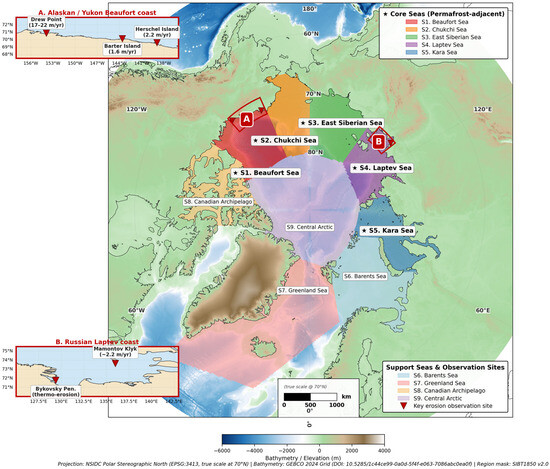
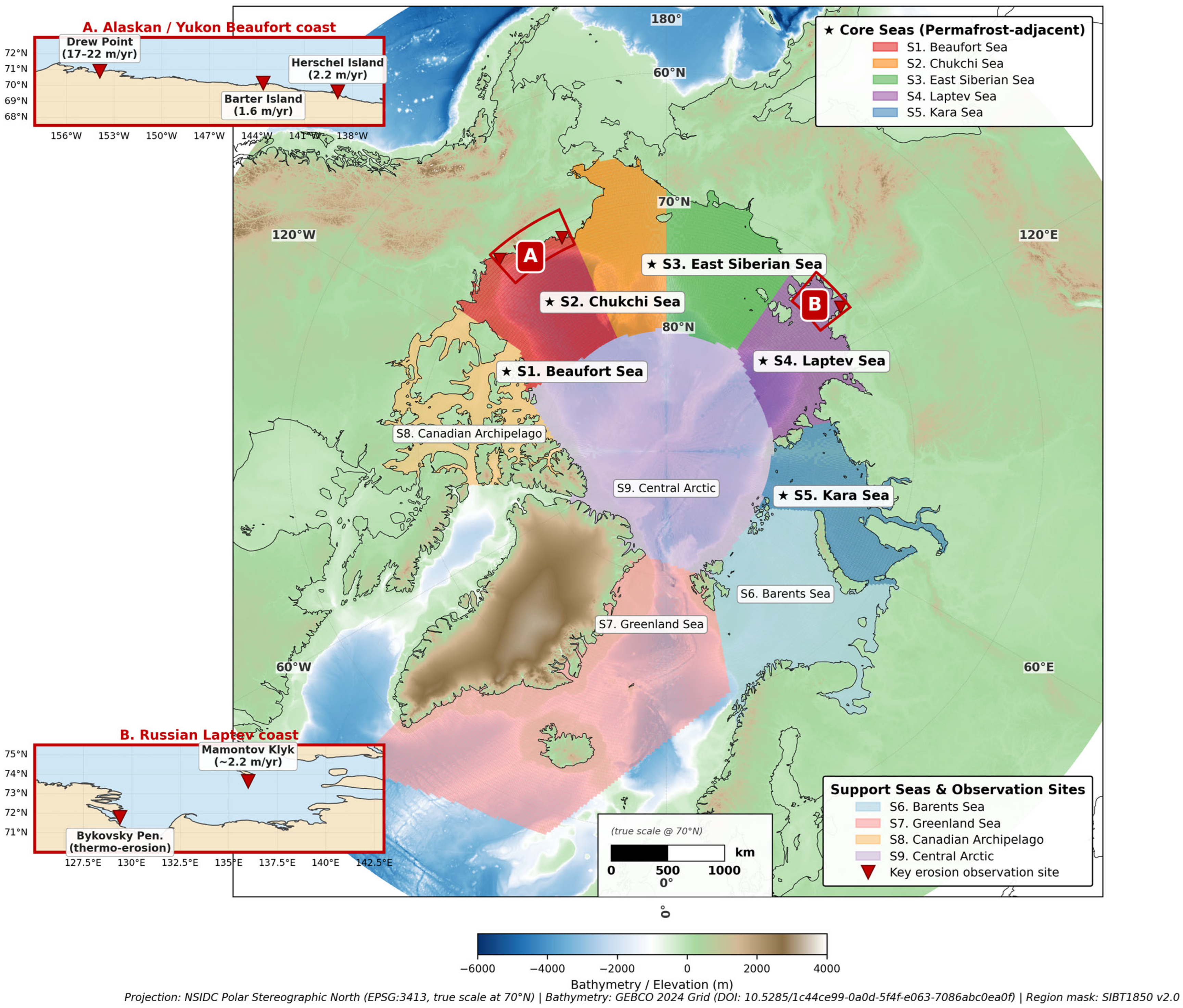
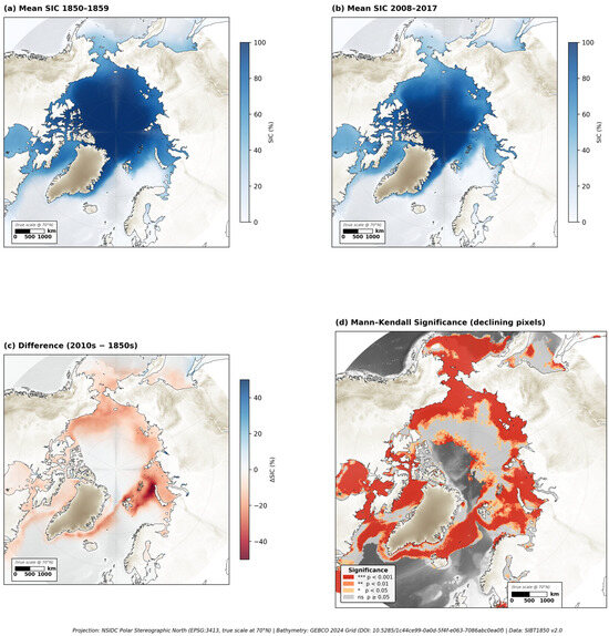
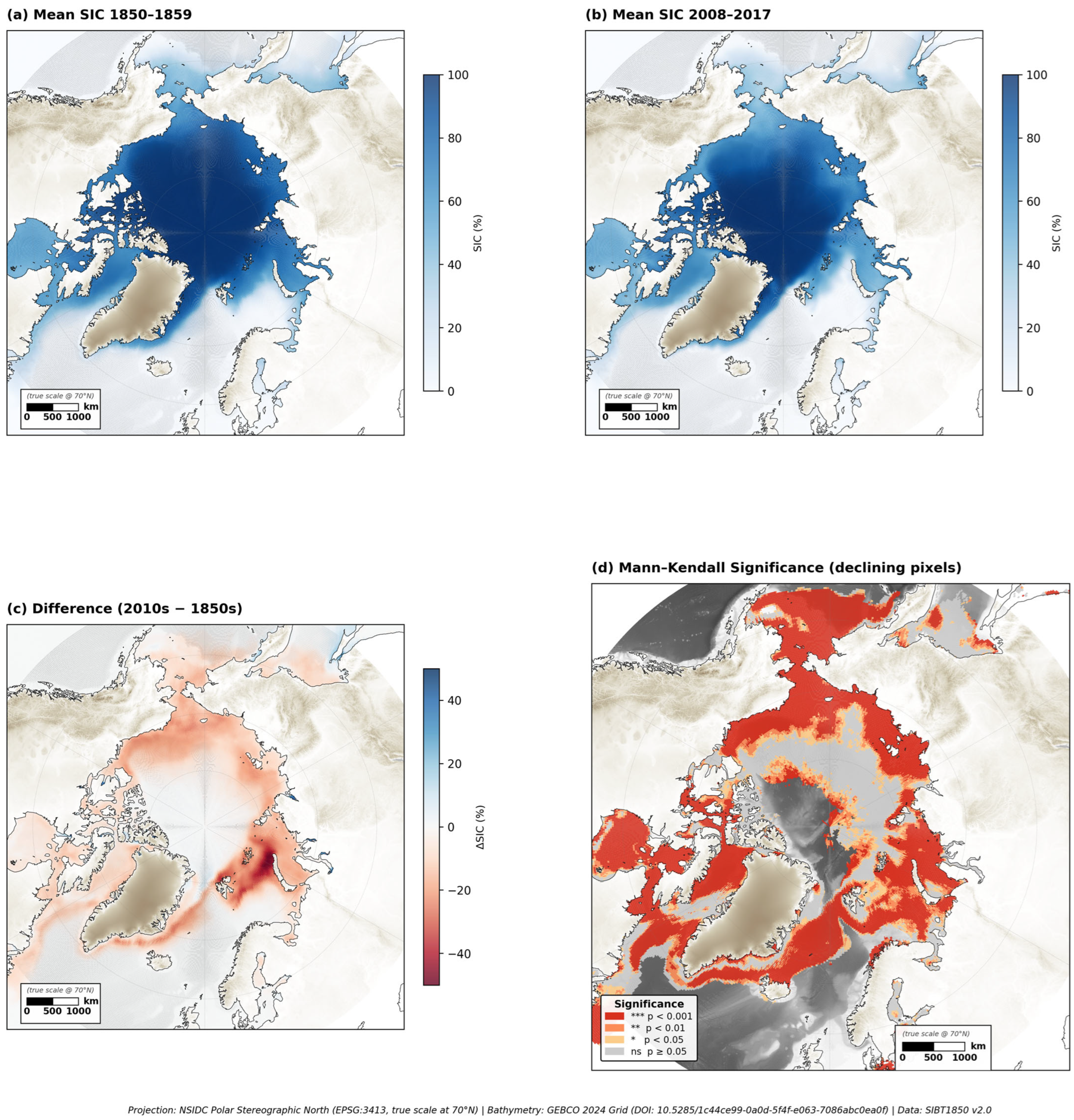
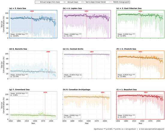
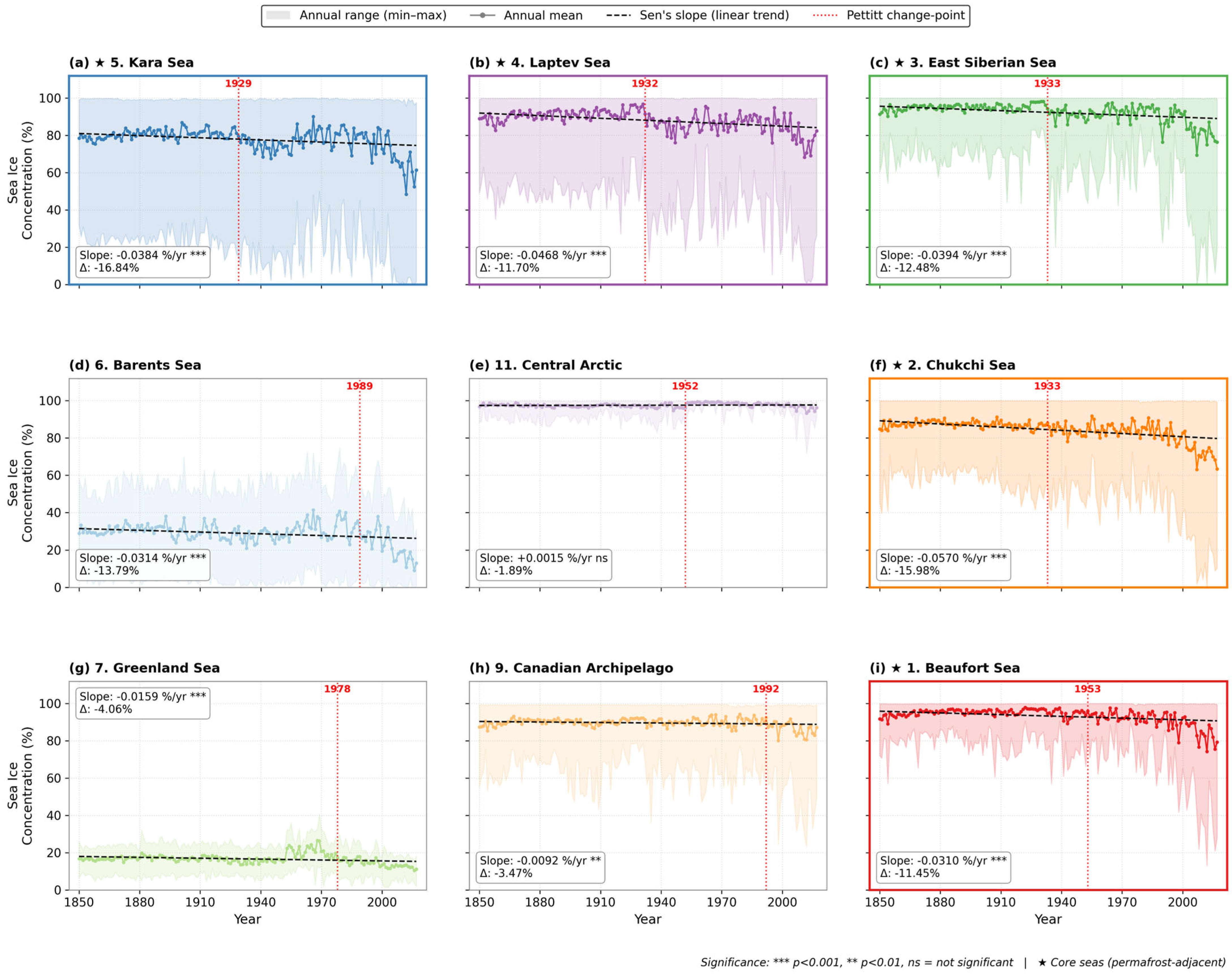
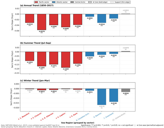
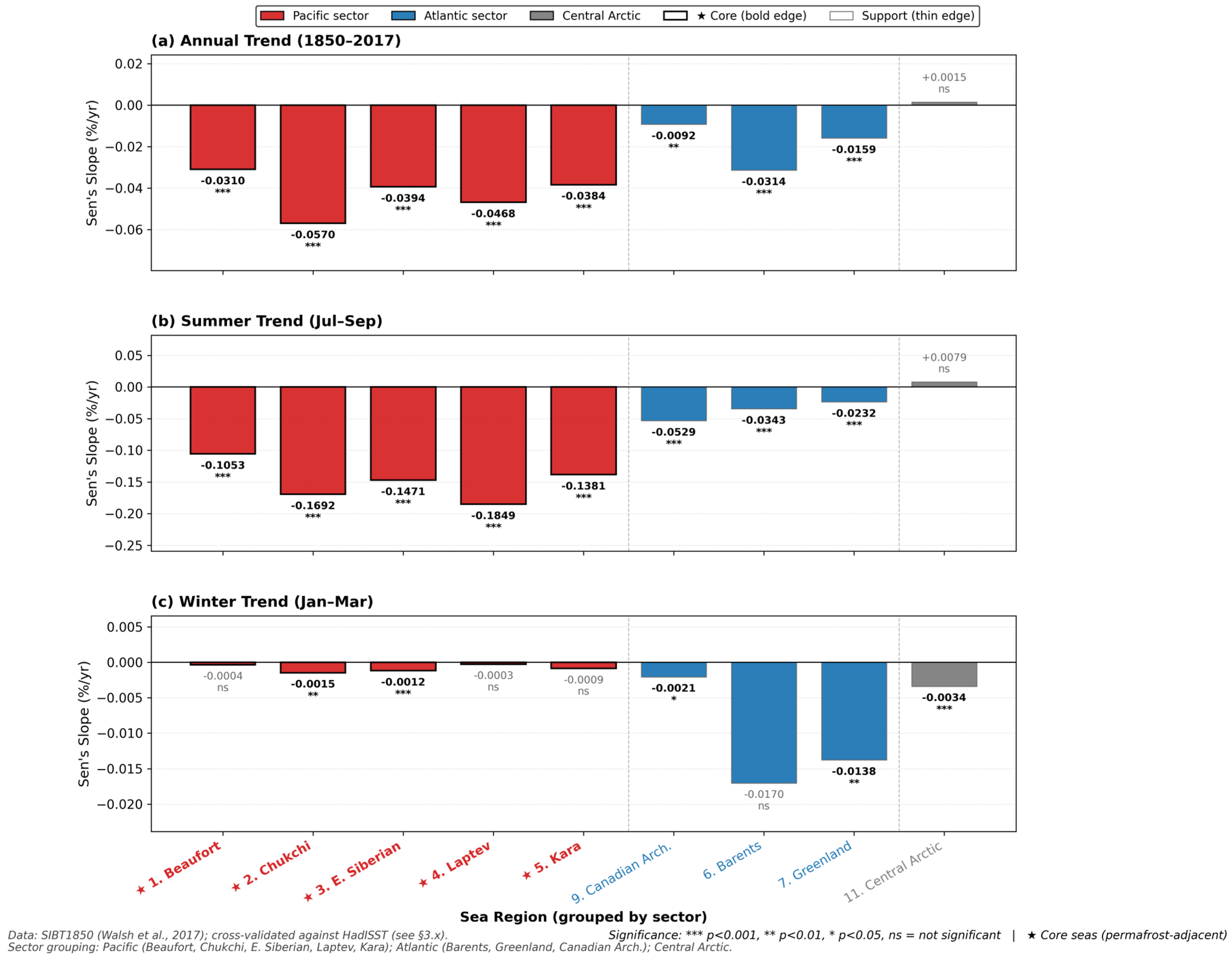
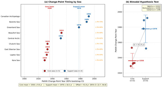
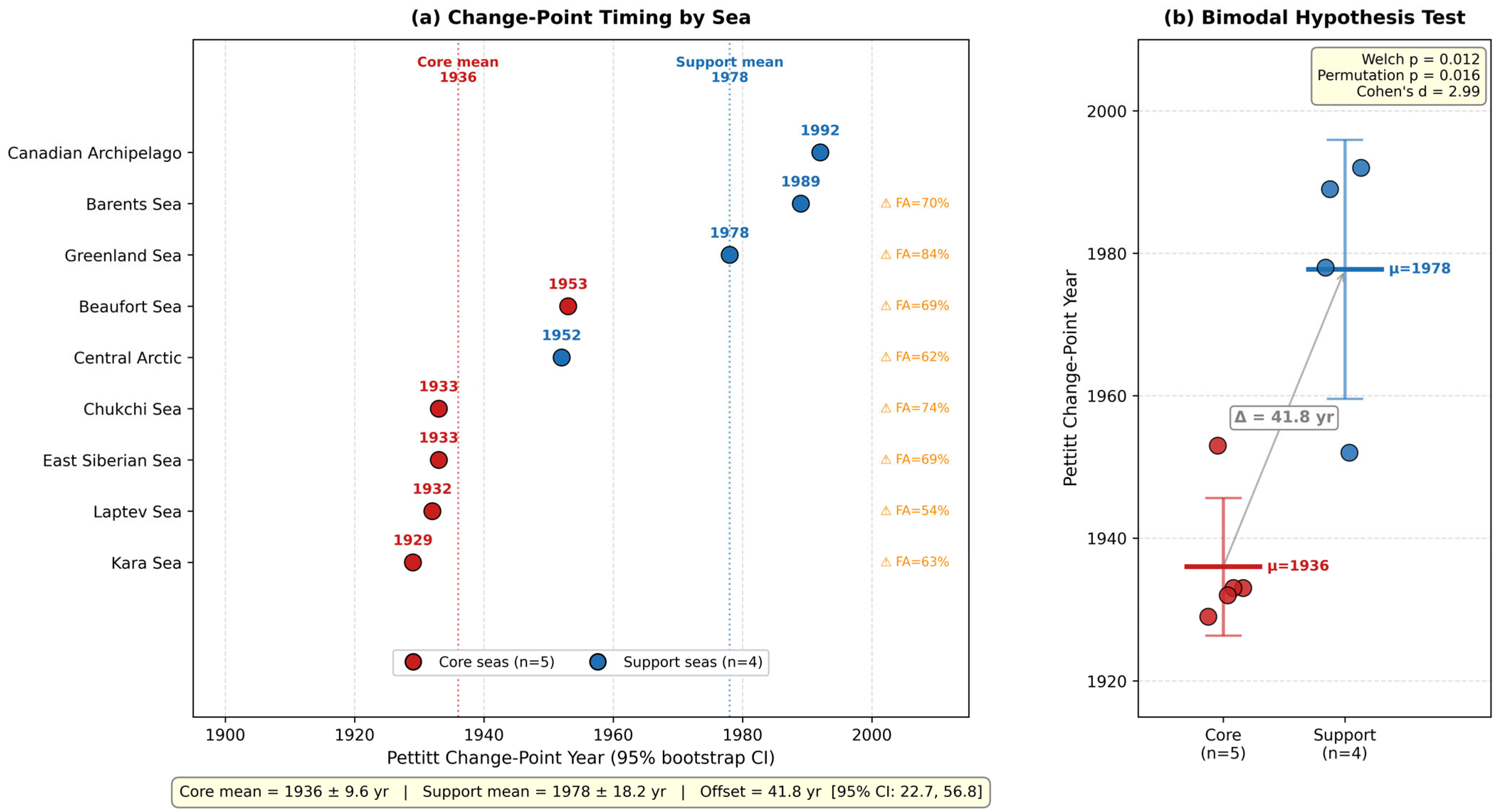
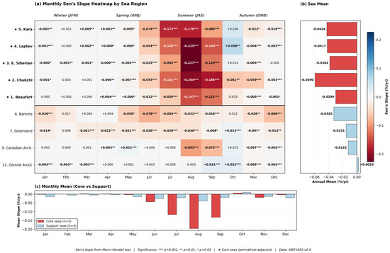
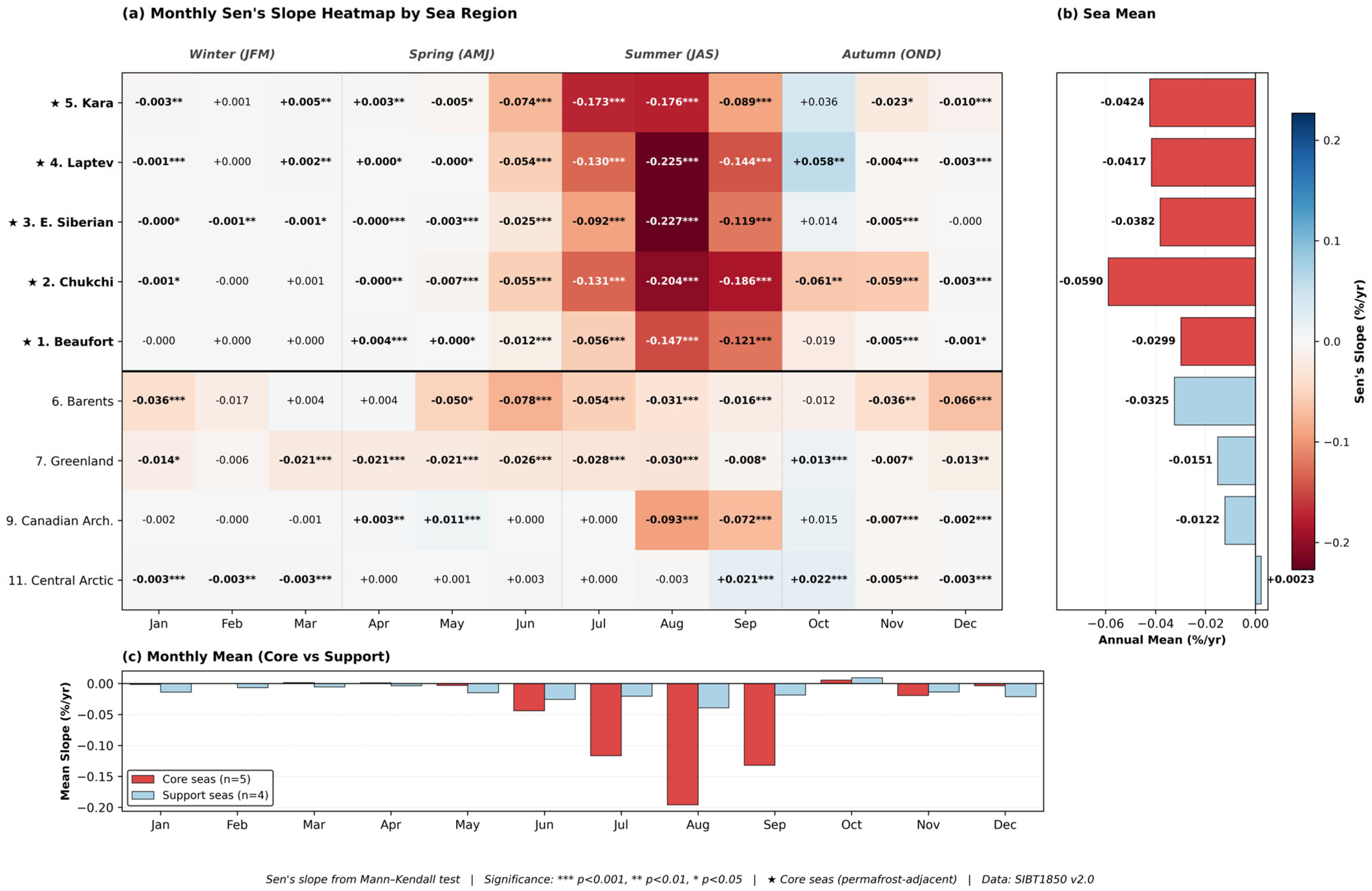
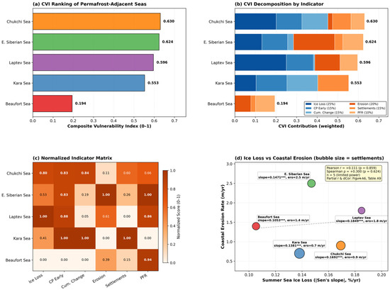
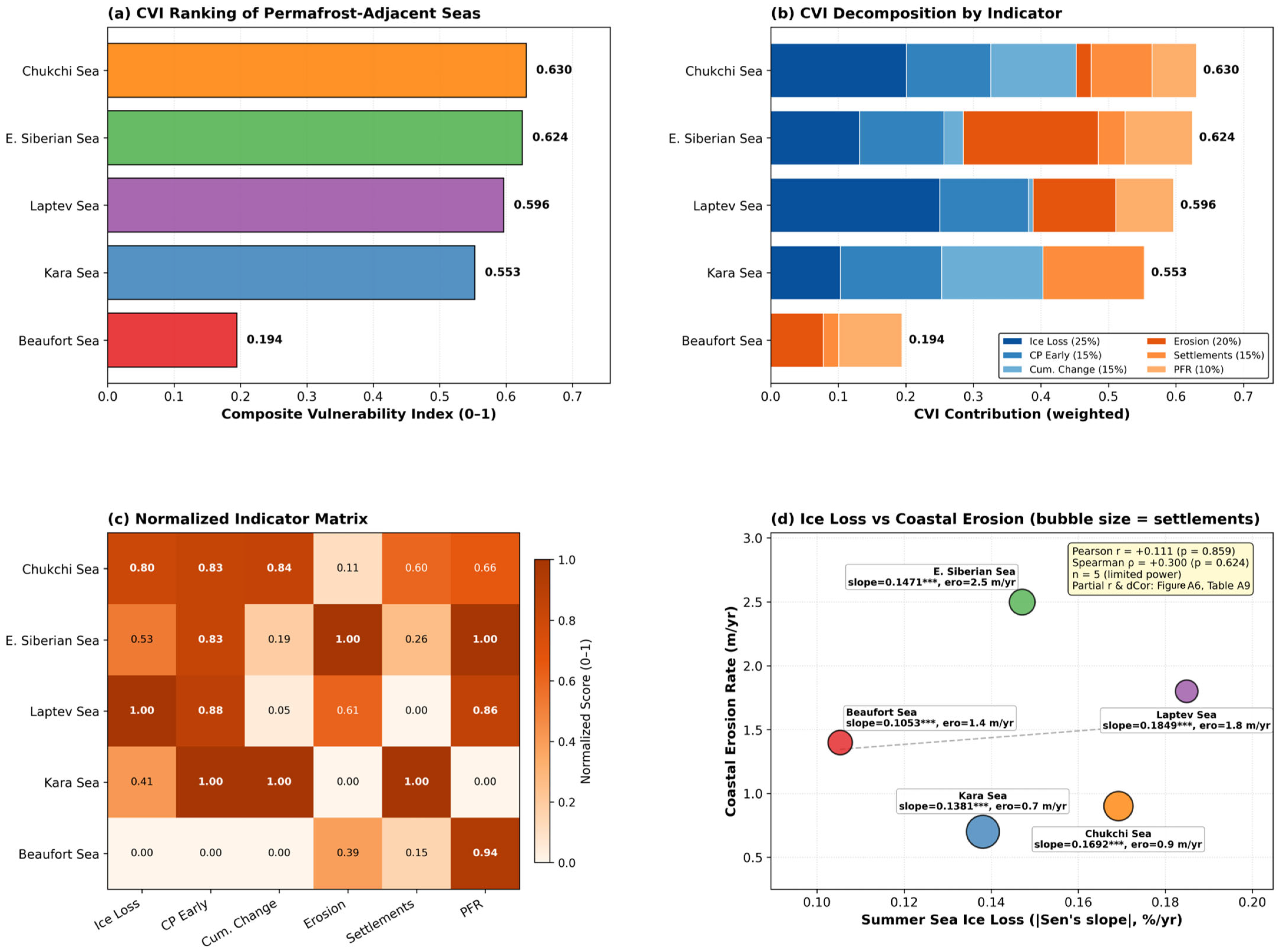

Disclaimer/Publisher’s Note: The statements, opinions and data contained in all publications are solely those of the individual author(s) and contributor(s) and not of MDPI and/or the editor(s). MDPI and/or the editor(s) disclaim responsibility for any injury to people or property resulting from any ideas, methods, instructions or products referred to in the content. |
© 2026 by the authors. Licensee MDPI, Basel, Switzerland. This article is an open access article distributed under the terms and conditions of the Creative Commons Attribution (CC BY) license.