


Abstract
Physics-based simulation of debris flows over complex terrain is essential for hazard assessment, but repeated numerical integration is costly when many scenarios must be explored. We develop a general deep-learning surrogate modelling framework for two-dimensional (2D) debris-flow propagation, here applied to the Morino–Rendinara area (central Italy) using a three-dimensional (3D) Fourier Neural Operator (FNO) trained on synthetic simulations generated by a validated in-house finite-volume shallow-water solver. The solver reproduces debris-flow propagation over complex terrain and is specifically developed for artificial intelligence (AI) applications. It is based on a depth-averaged 2D formulation using the Harten–Lax–van Leer–Contact (HLLC) approximate Riemann solver, hydrostatic reconstruction, positivity-preserving wet–dry treatment, and Voellmy-type basal friction, and was verified through analytical benchmarks, numerical tests, and back-analyses of real events. The dataset was built from four site-specific release settings derived from real topography, combining different released volumes and bulk densities while preserving local geomorphological and rheological characteristics. Each simulation was stored as a full spatio-temporal tensor and used to train an FNO conditioned on coordinates, topography, friction parameters, bulk density, and initial release thickness. Training used a novel loss to emphasize active-flow areas and improve velocity reconstruction, and was performed using a graphics processing unit (GPU). The surrogate shows effective generalization to within-distribution validation samples, with global relative mean squared errors of 5.49% for flow thickness, 5.34% for velocity component u, and 2.60% for v, and mean values of 0.95, 0.94, and 0.97. For a representative sample, the surrogate predicts the full spatio-temporal solution in s, versus about 47 s for the first-order finite-volume solver, corresponding to a speed-up of about , with an even larger gap expected for higher-order solvers, since, whilst the computation time of the solver increases as its complexity increases, the computation time of the FNO remains essentially unchanged. These results indicate that the proposed FNO is a reliable site-specific surrogate for rapid approximation of 2D debris-flow dynamics over real terrain, with potential for uncertainty propagation, Monte Carlo analysis, large-ensemble simulation, and hazard-oriented scenario assessment.
1. Introduction
Debris flows are among the most hazardous and complex mass-movement processes affecting steep mountainous areas, posing significant threats to human life, property, and infrastructure [1,2]. Their behaviour results from strongly nonlinear interactions among topographic forcing, granular–fluid rheology, sediment availability, and hydrological triggering, which makes reliable prediction intrinsically difficult [3,4,5]. For this reason, a broad hierarchy of numerical models has been developed to simulate debris-flow propagation, ranging from simplified one-dimensional (1D) depth-averaged formulations to fully two-dimensional continuum approaches [6].
Mathematical and numerical modelling is central to debris-flow research for process analysis, forecasting, and impact assessment. These models are generally based on mass and momentum conservation, with constitutive or empirical closure relations. Computational Fluid Dynamics (CFDs) [7,8] provides detailed simulations, but its fully 3D formulations are computationally demanding; hence, shallow-water models are widely adopted [9,10,11].
The governing equations are solved by discretizing the computational domain, allowing the evolution of stress, velocity, and flow thickness to be computed. Common approaches include the Finite Element Method (FEM) [12], the Finite Volume Method (FVM) [13], Smoothed Particle Hydrodynamics (SPHs) [14,15], and the Particle Finite Element Method (PFEM) [16,17]. Despite major advances, these solvers remain computationally demanding and may face stability issues over steep and irregular terrain, as well as in wet–dry transitions and rapidly evolving flows [18,19].
Comparative studies show that different simulation codes can reproduce observed runout and deposition [20,21,22,23,24,25,26], though results remain sensitive to rheological assumptions and topographic resolution [27,28,29]. Many advanced solvers, including FLO-2D PRO, RAMMS, and DAN3D, are also proprietary and require paid licences [30,31,32], which may limit methodological transparency, hinder reproducibility, and, more broadly, constrain scientific progress. This, together with the limited availability of observational debris-flow datasets, restricts the use of purely data-driven machine-learning approaches, which generally require large labelled datasets.
Recent studies identify surrogate modelling, especially operator-learning techniques, as a promising way to address these limitations [33,34,35,36]. By approximating the input–output mapping of numerical solvers, surrogate models reduce computational cost while retaining physical consistency when trained on synthetic or observational data [37]. Within this framework, Fourier Neural Operators (FNOs) have emerged as effective tools for learning solution operators and approximating parametric partial differential equations efficiently [38,39,40]. They have already shown strong performance in advection–diffusion and geophysical transport problems, enabling stable, mesh-independent, and near-instantaneous predictions of full space–time fields.
Previous work showed that FNOs can model debris flows in simplified 1D settings, reproducing a validated 1D shallow-flow solver with solid accuracy at much lower computational cost [41]. However, this framework cannot represent lateral spreading, cross-slope velocities, or explicit 2D geomorphological controls on deposition, motivating a fully 2D formulation.
In this study, we extend the FNO to 2D debris-flow modelling in a hazard-oriented framework. We develop and assess a physics-based surrogate, trained on synthetic simulations, to reproduce debris-flow dynamics over real terrain in space and time. Training data are generated with a validated 2D shallow-flow solver, allowing the model to learn the spatio-temporal evolution of flow thickness and depth-averaged velocity under varying topographic and physical conditions. In the absence of large real spatio-temporal datasets, the use of a numerical solver validated against real calibrated events provides a physically grounded way to generate synthetic simulations suitable for training the surrogate model.
The study is also motivated by the need to support susceptibility assessment in areas exposed to hydrogeological hazards, especially where debris flows may threaten residential sectors and local infrastructure. The March 2021 Morino–Rendinara event [6] represents a significant example of a hydrogeological hazard, having mobilized several hundred cubic metres of material, partially obstructing the Liri riverbed, and exposing nearby infrastructure to the rapid propagation of debris flows. Accordingly, this area will serve as a reference site for the development of site-specific hazard-oriented simulations within the basin.
The work addresses two main challenges: the scarcity of high-quality observational data and the computational cost of traditional solvers. To this end, simulations are performed on local 2D domains embedded in the 3D topography of the Rendinara–Morino area, while preserving its main geomorphological features and detachment configurations.
For this reason, the present study relies on an in-house numerical solver designed both to reproduce debris-flow propagation over complex terrain and to generate physically consistent outputs directly usable for dataset construction, storage, and AI training. Achieving the same level of control and integration with external codes would have been far more cumbersome. These data are then used to train a dynamic 3D Fourier Neural Operator (FNO) model in , conditioned on terrain, friction, bulk density, and initial detachment conditions, with training performed using GPU acceleration.
Compared with earlier 1D studies, the present 2D formulation captures lateral spreading, channelization, and planimetric deposition, while introducing greater sensitivity to topographic complexity and wet–dry fronts. We also examine the training objective by adopting a masked and weighted loss that emphasizes active-flow regions and velocity reconstruction, both especially relevant for hazard-oriented applications.
The main objective is to propose a fast and general surrogate-modelling framework for solver-consistent landslide runout simulations, and to demonstrate its application through the Morino–Rendinara case study. In this context, the trained surrogate developed here is specifically tailored to the Morino–Rendinara geomorphological setting and to the parameter space explored in this study; as such, it should be interpreted as a Morino-specific model rather than a universally transferable trained model. Nevertheless, the overall framework is general and can be applied to other study areas, provided that appropriate site-specific training datasets are generated to capture the relevant geomorphological features and parameter ranges. This approach may support location-specific surrogate models for debris-flow hazard assessment, providing efficient predictions consistent with numerical solvers and tailored to individual catchments. The expected computational advantage is relevant not only for large scenario ensembles and uncertainty analyses, but also for single simulations, suggesting possible integration with monitoring networks in operational early-warning frameworks for hydrogeological risk.
2. Study Area
This section presents the characterization of the Morino–Rendinara area (Figure 1), which we aim to represent using the FNO model. The objective is to describe the geomorphological and physical attributes of this debris-flow system in a form suitable for integration within an FNO framework.
Figure 1.
(a) The Roveto Valley, located in the Abruzzo Region (Italy); (b) Zoomed-in map of the landslide extension in the Rio Sonno/Fiume Liri area [6].
The synthetic dataset developed in this work was inspired by the debris-flow event that occurred in March 2021 in the Morino–Rendinara area (Abruzzo Region, central Italy), along the Rio Sonno channel, a tributary of the Liri River [6]. The study area is located near the hamlet of Rendinara, within the Municipality of Morino, in the upper part of the Roveto Valley on the eastern side of the Liri River valley [6]. During the March 2021 event, several hundred cubic metres of material were mobilized, partially obstructing the Liri riverbed and temporarily altering the local hydrogeological regime [6].
3. Materials and Methods
3.1. Physical Model: 2D Governing Equations for Debris-Flow Modelling
Debris-flow propagation is described here within a depth-averaged 2D framework, in which the moving mass is represented as a shallow continuum flowing over a prescribed topography. Under the shallow-flow assumption, the characteristic flow thickness is small compared with the typical horizontal length scale, so that the full 3D problem can be reduced to a system of depth-integrated balance equations. This approximation is well suited for rapid gravity-driven flows over natural terrain, where the dominant controls are topographic forcing, hydrostatic pressure gradients, and basal resistance. In the present formulation, the bulk density is treated as a material property and is assumed to be spatially uniform and temporally constant. In our physical model, this assumption is a simplification of the real process, since actual debris flows may exhibit spatial and temporal variations.
Let denote the bed elevation, the flow thickness, and the depth-averaged velocity components in the horizontal directions x and y. The free-surface elevation is defined as
From a physical point of view, the debris flow is governed by depth-integrated conservation of mass and momentum. The continuity equation reads
where represents a possible external inflow contribution and E denotes the erosion–entrainment rate. Phase segregation is not explicitly modelled; deposition is assumed when the local depth-averaged velocity tends to zero.
The corresponding momentum equations in the two horizontal directions are
where g is the gravitational acceleration, and and are the basal shear-stress components acting along the two horizontal directions.
Equations (2)–(4) show the main physical mechanisms controlling debris-flow propagation: conservation of mass, advection of momentum, hydrostatic pressure forces, gravitational forcing induced by bed gradients, and basal resistance. In particular, the terms and represent the driving effect of the terrain, whereas the basal shear stresses oppose the motion and describe the rheological resistance of the flowing mass.
For compactness, the same system can be written in conservative vector form by introducing the vector of conserved variables
so that
where and are the depth-integrated flux vectors and collects the source terms associated with bed slope, basal resistance, inflow, and erosion–entrainment.
The flux vectors are
and the source-term vector may be written formally as
For the Morino–Rendinara zone, consistently with [6], basal resistance is represented through a Voellmy-type [42] combining a Coulomb-like frictional contribution with a velocity-dependent turbulent term. The basal shear-stress magnitude is written as
where is the dry-friction coefficient, is the turbulent friction parameter, is the flow speed, and is the effective normal acceleration. In the absence of curvature corrections, the latter reduces to
where is the local slope angle. More generally, if curvature effects are taken into account, the effective normal acceleration may be written as
where is a curvature-related contribution depending on the local velocity field and terrain curvature.
To obtain the Cartesian components entering the momentum equations, the basal shear stress is projected along the flow direction as
where is a small regularization parameter introduced to avoid division by zero in nearly stagnant cells.
Depending on the modelling assumptions, the mass balance may also include localized external supply terms and entrainment from the bed. In the latter case, erosion–entrainment is commonly activated when the basal shear stress exceeds a critical threshold [43]. A simple threshold-based entrainment law may therefore be written as
where is an empirical entrainment coefficient. Equivalently, the same relation may be expressed in compact form as
This expression indicates that erosion begins only when the basal stress exceeds the critical threshold, and subsequently increases with the excess shear stress, which can also be addressed within a probabilistic framework [44].
The physical problem is completed by appropriate initial and boundary conditions. The initial condition specifies the starting distribution of flow thickness and momentum within the computational domain and may represent either an instantaneous release or a time-dependent supply of material.
3.2. Numerical Solver: Finite-Volume Scheme
The full numerical formulation of our in-house solver is reported in Appendix A.1. In the present implementation, the solver adopts a depth-averaged shallow-flow formulation with spatially uniform and temporally constant bulk density, Voellmy-type basal friction with spatially distinct selectable basal-friction regions consistently with [6], threshold-based erosion–entrainment, no explicit phase segregation, and deposition assumed to occur as the local depth-averaged velocity approaches zero. The depth-averaged equations introduced above are solved with a finite-volume scheme on a structured Cartesian grid derived from the DEM. Conserved variables are stored as cell averages and updated from intercell numerical fluxes and source terms. The scheme is designed to remain stable over irregular topography, preserve non-negative flow thickness, and handle wet–dry transitions consistently.
To balance accuracy and robustness, the solver adopts a higher-order treatment in regular flow conditions and a more diffusive formulation near locally critical states. Time integration is explicit and satisfies a Courant–Friedrichs–Lewy (CFL) stability condition. This makes the method efficient and robust for generating a large ensemble of synthetic simulations used to train the surrogate model.
The full numerical formulation reported in Appendix A.1 includes the finite-volume update, approximate Riemann solver, hydrostatic reconstruction, Monotonic Upstream-centred Schemes for Conservation Laws (MUSCL), hybrid first–second–order strategy, time integration, and wet–dry treatment. Solver validation is presented in Appendix A.2, including analytical benchmarks in Appendix A.2.1 and Appendix A.2.2, convergence tests in Appendix A.2.3, conservation tests in Appendix A.2.4, and comparisons with real debris-flow case studies in Appendix A.3.
An important real-case validation is provided by the Morino–Rendinara debris flow, which was reproduced and compared with the back-analysis of Pasculli et al. [6]. In their study, the event was simulated using RAMMS v1.5, adopting a shallow-water model coupled with a Voellmy-type rheology. They reported a flow thickness of about . Using the same input parameters, our simulation showed significant agreement with the observed evidence. Further details are given in Appendix A.3.1.
3.3. Dataset Parameter Space and Numerical Setup
The synthetic dataset was generated by repeatedly solving the debris-flow model on local domains extracted from the Morino–Rendinara area, reproducing the main geomorphological controls of the study area. Four representative release profiles were selected to sample different site-specific conditions (Figure 2). These four release profiles were chosen to represent different source areas and debris-flow paths in the Morino–Rendinara basin, considering local topography, release geometry, and deposition patterns affecting Rendinara and Morino. Together, they provide a compact but varied set of site-specific scenarios to characterize urban boundaries from a debris-flow hazard perspective, rather than to cover all possible source areas in the basin. Since the training set is produced by our validated numerical solver, the synthetic simulations are not arbitrary realizations, but physically consistent solutions of the adopted debris-flow model under site-specific topographic and rheological conditions.
Figure 2.
Summary of the release locations used for synthetic dataset generation in the Morino–Rendinara area.
All simulations were performed on a digital elevation model (DEM) resampled to a 10 m resolution. The governing equations were integrated up to s with the finite-volume solver described above, employing a first-order scheme to limit computational cost, explicit time stepping, and a CFL-based stability criterion. Outputs were stored every 10 s to obtain a time-resolved description of the flow evolution. In order to limit the computational burden, curvature effects and inflow hydrographs were neglected; the simulations therefore represent release-driven propagation governed solely by topography, Voellmy-type basal friction, and erosion–entrainment. One representative finite-volume simulation required approximately 47 s, providing a reference cost for comparison with surrogate inference. The finite-volume simulations used for dataset generation were carried out on Google Colab in a Python 3.12 environment, using a cloud-based runtime equipped with an NVIDIA RTX PRO 6000 Blackwell Server Edition GPU.
The parameter space was kept compact and focused on the main controls on event intensity. The basal-friction parameters were fixed according to the values adopted for the real Morino–Rendinara case, namely , , and , consistently with Pasculli et al. [6]. In contrast, bulk density and released volume were varied systematically. In particular, the dataset includes different hypothetical release volumes, introduced to represent debris-flow scenarios of increasing magnitude. Larger volumes are expected to produce longer runout distances and greater deposited thicknesses, while different bulk-density values were considered to account for plausible variations in flow inertia. The initial condition of each simulation is defined by the released volume V and the initial thickness field . The latter is prescribed within the release polygon, so that the source geometry defines the spatial support of the initial mass, while the hypothetical release volume controls its magnitude. Boundary conditions were kept fixed throughout the campaign and coincide with those of the numerical solver: an open-domain treatment was adopted, and no external inflow was prescribed. Four release settings were considered. For each of them, simulations were generated by combining five bulk-density values, and , with five hypothetical release volumes equal to and . This produced 25 simulations for each release setting and 100 simulations in total. For the present site-specific objective, this 100-sample dataset was considered adequate because it systematically covers the four release profiles of interest and the main volume–density combinations controlling event magnitude.
A summary of the main simulation parameters is reported in Table 1.
Table 1.
Parameter space and numerical setup adopted for the generation of the synthetic debris-flow dataset in the Morino–Rendinara area.
Figure 2 summarizes the spatial distribution of the four release settings within the Morino–Rendinara area. The dataset therefore does not rely on a single terrain configuration, but samples multiple site-specific propagation contexts.
For each simulation, solver outputs were converted into train-ready tensors. The stored channels include topography, basal-friction maps, time-dependent flow variables, and bulk density as conditioning information. Since the local domains differ in spatial extent, all samples were padded to a common tensor size and stored. The train–validation split was performed with a balanced procedure to ensure that all release settings were represented in both subsets. A validation fraction of was adopted, together with a fixed random seed for reproducibility. A summary of the dataset characteristics is reported in Table 2.
Table 2.
Structural characteristics of the synthetic dataset and numerical setup adopted for FNO training.
To clarify the internal organization of the dataset, two representative release settings are discussed in more detail: Release 2 and Release 4. These correspond to two of the four release profiles adopted in the synthetic campaign.
Figure 3 shows the orthophoto-based configuration of the two selected profiles. In each case, the maps identify the release location, the release polygon, the clipping window used to define the local computational domain, and the two friction polygons adopted to represent the spatial variability of basal resistance in the Morino–Rendinara area. Each release scenario is therefore defined not only by a source location, but also by a specific domain geometry and friction zoning.
Figure 3.
Detailed spatial configuration of Release 2 (a) and Release 4 (b) in the Morino–Rendinara dataset.
To complement the geometric description, two representative simulations are shown for the same release settings. Figure 4 reports the final simulation frames at for Release 2 and Release 4, for virtual released volumes of and , respectively.
Figure 4.
Final flow-thickness maps for Release 2 (a) and Release 4 (b) at , for virtual released volumes of and , respectively.
The plotted variable is the final flow thickness h, superimposed on the local hillshade topography. These examples illustrate the type of spatio-temporal output stored in the dataset. Although the simulations share the same numerical framework, the resulting runout and deposition patterns differ because of the different local topography, release geometry, and friction zoning associated with each profile. Only the final flow-thickness field h is shown here, although the solver also provides the 2D velocity components u and v for each simulation output; these are analyzed in greater detail in Section 4.
3.4. Fourier Neural Operator
The FNO is an AI-based method that has emerged as an effective architecture for learning mappings between function spaces arising in physical systems [38,40]. Instead of approximating a single solution for a fixed configuration, neural operators learn an operator that maps input functions, such as parameters, geometry, or initial conditions, to the corresponding solution fields.
In the context of debris-flow modelling, the objective is to learn the nonlinear operator
where represents the set of input fields and conditioning parameters (e.g., topography, rheological parameters, and initial conditions), and denotes the resulting flow variables predicted by the model. Similar ideas have recently been explored in debris-flow applications [41], where deep learning was used to approximate the dynamics generated by shallow-flow numerical solvers.
The key idea of the FNO is to perform the learning process in the spectral domain. By operating in the Fourier domain, the model can capture long-range spatial interactions with a reduced number of spectral coefficients, which is particularly advantageous for fluid-dynamical and geophysical flow problems [33,38,40].
Figure 5 [38] illustrates the structure of the FNO used in this work. Figure 5a shows the overall architecture: the input function is first mapped to a higher-dimensional representation through a lifting operator P, then processed through multiple Fourier layers, and finally projected back to the physical variables through a projection operator Q. Figure 5b shows the internal structure of a Fourier layer, where the feature maps are transformed into Fourier space, modified by learnable spectral weights, and combined with a local linear transformation before the nonlinear activation.
Figure 5.
Architecture of the FNO used to approximate the debris-flow solution operator. (a) Global structure of the network. (b) Internal structure of a Fourier layer [38].
Once trained, the FNO provides a fast surrogate of the numerical solver, capable of predicting the spatio-temporal evolution of the debris-flow fields for new input configurations. This capability makes neural operators particularly attractive for large ensemble simulations, uncertainty propagation, and rapid scenario analysis in debris-flow hazard assessment.
3.5. Training Procedure and Model Optimization
The FNO was trained to approximate the nonlinear mapping between the spatio-temporal fields defining each synthetic debris-flow scenario and the corresponding evolution of the simulated flow variables. In the present dataset, each sample is stored as a tensor of shape , where the seven channels correspond to the basal friction coefficient , the turbulent friction parameter , the bulk density , the bed elevation , the flow thickness h, and the two depth-averaged velocity components u and v.
Starting from these fields, the input tensor of the neural operator is constructed by combining normalized coordinates with the physical conditioning variables. More precisely, the network input is defined as
where denotes the initial flow thickness, replicated along the temporal dimension. The network target is instead given by
Therefore, the model learns the full spatio-temporal evolution of the depth and velocity fields from the geometric, rheological, and initial-condition descriptors of the problem.
A summary of input and output variables used for FNO training is reported in Table 3.
Table 3.
Input and output variables used for FNO training.
Before training, channel-wise normalization statistics were computed using only the training subset. The normalization was applied separately to the physical input channels and to the output channels , whereas the coordinates were already expressed in normalized form in the interval . Means and standard deviations were estimated globally over the valid cells of the training samples only, so that padded regions did not influence the statistics. The same normalization parameters were then used consistently for both training and validation data.
The surrogate model is a 3D FNO acting jointly on the two spatial coordinates and on time. The network receives tensors of shape
where B denotes the batch size, and returns tensors of shape
The architecture first lifts the eight-dimensional input into a latent feature space of width 96 through a fully connected layer. The latent representation is then processed by three consecutive Fourier blocks, a choice based on initial tuning experiments and practical GPU memory constraints, and retained as a sufficiently expressive and stable compromise between predictive accuracy, computational cost, and training robustness. Each block combines a spectral convolution in the domain with a pointwise convolution, followed by a Gaussian Error Linear Unit (GELU) activation function. In the spectral branch, only a truncated set of Fourier modes is retained, namely 16 modes along each spatial direction and 12 modes along the temporal direction. After the sequence of Fourier blocks, the latent representation is projected back to the physical output space by means of two fully connected layers, with an intermediate projection dimension equal to 160. In order to reduce edge artefacts during the spectral operations, a padding of five cells is applied before the Fourier blocks and removed after the spectral processing. The model parameters were optimized using the Adam algorithm with an initial learning rate equal to and weight decay equal to . Training was performed for 100 epochs with a batch size equal to 1 for both training and validation. The learning rate was updated through a multi-step scheduler, with decay milestones at epochs 60 and 80 and multiplicative factor . At the end of each epoch, the model was evaluated on the validation set, and the best-performing checkpoint was selected according to the minimum validation loss.
A standard training loss, such as mean squared error, mean absolute error, or Huber loss, can be dominated by the many dry or nearly dry cells present in each simulation. As a result, it may achieve effective overall accuracy while still under-resolving the advancing front and the sparse regions with active flow. To address this issue, the training objective was defined as a task-specific masked loss designed to exclude padded cells, emphasize active-flow regions, and assign greater importance to velocity reconstruction. In the main text, we report only the global form of the objective function, while the detailed definitions of the channel-wise loss terms are provided in Appendix A.4.
Accordingly, the total training loss is written as
with
The detailed formulation of , , and , including the masking and weighting strategy adopted for active-flow regions and padded cells, is reported in Appendix A.4. This choice was introduced to assign greater importance to the reconstruction of the velocity field, which is generally more difficult to learn and more sensitive to localized discrepancies near the advancing front and in low-thickness regions [41].
During training, the trend of the total loss and of the individual channel-wise contributions was stored for both training and validation. In addition, model checkpoints, optimizer state, scheduler state, and normalization parameters were periodically saved in order to ensure reproducibility and restart capability. At the end of the optimization process, both the final model and the model achieving the minimum validation loss were exported and retained for subsequent evaluation.
The model was trained in the same Google Colab computing environment used for finite-volume simulations and dataset generation, with Python 3.12, using a cloud-based runtime equipped with an NVIDIA RTX PRO 6000 Blackwell Server Edition GPU. The total training time was approximately 2 h 30 min.
A summary of the architecture, loss weighting, optimization, and training setup of the 3D FNO adopted in this work is reported in Table 4.
Table 4.
Architecture, loss weighting, optimization, and training setup of the 3D FNO adopted in this work.
4. Results
4.1. Training Dynamics and Validation Errors
The training and validation loss trends for the total objective function, flow thickness h, and velocity components u and v are shown in Figure 6. Overall, the optimization process exhibits stable convergence over the 100 training epochs. All loss terms decrease rapidly during the initial epochs, followed by a slower decay toward convergence.
Figure 6.
Training and validation loss histories for (a) the total loss, (b) the flow thickness h, (c) the velocity component u, and (d) the velocity component v.
A close agreement between training and validation curves is observed for all monitored quantities. This behaviour indicates satisfactory generalization to within-distribution validation samples and no significant overfitting.
For the quantitative assessment, model performance was evaluated using the masked mean squared error (MSE) and the relative masked mean squared error (rMSE), both computed over the valid spatio-temporal support of each sample [45,46].
At the dataset level, the validation results confirm the overall robustness of the model. The mean relative mean squared error is 5.49% for the flow thickness h, 5.34% for the longitudinal velocity u, and 2.60% for the transverse velocity component v. The corresponding average coefficients of determination are , , and , respectively. Overall, the surrogate reconstructs all three target fields with significant accuracy on the validation set, with particularly strong performance for the transverse velocity component v, which shows the lowest relative error and the highest . Although the absolute MSE values reported in Table 5 are larger for the velocity components than for flow thickness, this does not imply worse normalized reconstruction accuracy, since h, u, and v differ in physical units, characteristic magnitude, and spatial variability. This is confirmed by the relative MSE values, which are very similar for h and u (5.49% and 5.34%, respectively) and lower for v (2.60%), indicating that the normalized reconstruction of the transverse velocity component is, overall, more accurate. In addition, the difference between u and v likely reflects their different morphodynamic roles within the flow, with u more directly associated with channelized downslope propagation and localized acceleration along the main flow path, and v more influenced by lateral spreading, local curvature, and channel widening or narrowing. In practical terms, these error values indicate that the surrogate model reproduces the target fields with solid accuracy on the validation set. The corresponding quantitative metrics are summarized in Table 5.
Table 5.
Global validation errors of the surrogate model for flow thickness and velocity components. Reported metrics include the MSE (in m2 for h and m2 s−2 for u and v), the rMSE (adimensional), and the corresponding percentage form of rMSE.
To complement the aggregate validation metrics reported in Table 5, which summarize the mean performance over the full validation set, Table 6 presents the corresponding sample-wise validation results for all validation samples at the final simulation time. This more detailed view makes it possible to assess not only the overall average behaviour of the surrogate, but also the spread of errors across individual cases, including the less accurate and more demanding samples. In particular, the relative mean squared error ranges from 0.54% to 11.15% for h, from 1.39% to 9.46% for u, and from 1.62% to 3.63% for v, with corresponding values ranging from 0.86 to 0.99, 0.90 to 0.98, and 0.96 to 0.98, respectively. These results indicate that the transverse velocity component v is reconstructed more consistently across the full validation set, whereas the largest sample-to-sample variability is observed for flow thickness h and, to a lesser extent, for the longitudinal velocity u.
Table 6.
Sample-wise validation metrics for all validation samples at the final simulation time, sorted by decreasing relative mean squared error for the flow-depth field h.
In addition to predictive accuracy, the surrogate also provides a substantial reduction in computational cost at inference time. For a representative validation sample, the trained FNO required only s to predict the full spatio-temporal solution, whereas the corresponding numerical simulation performed with the first-order finite-volume solver on the same 10 m DEM required approximately 47 s. Both timings therefore refer to the same Google Colab computing environment, avoiding a comparison between different hardware configurations. This corresponds to a speed-up factor of about compared with the first-order finite-volume solver (Table 7).
Table 7.
Representative times for solver execution and surrogate inference for the same sample.
4.2. Final Flow-Depth Maps for Representative Validation Samples
To complement the aggregate validation metrics reported in Section 4.1, the surrogate was further analyzed on three representative validation samples: sample_000029 (released volume 750 m3), sample_000079 (released volume 750 m3), and sample_000045 (released volume 1000 m3). These cases were selected to compare different local release settings and to highlight different levels of reconstruction difficulty, including the most challenging validation case for the final flow-depth field h.
Table 8 summarizes the sample-wise validation errors for the final flow thickness field h. For sample_000029, the relative mean squared error is with , whereas for sample_000079 the relative mean squared error is with . By contrast, sample_000045 yields a relative mean squared error of with , and therefore represents the most demanding validation case for the final flow-depth field among the validation samples. These results indicate that the surrogate reconstructs the final flow thickness with very effective accuracy in the first two cases, while sample_000045 provides a useful example of a more challenging prediction setting.
Table 8.
Sample-wise validation metrics for the final flow thickness h in three representative validation cases.
Figure 7, Figure 8 and Figure 9 compare the reference and predicted final flow thickness h for the three validation samples. For sample_000029 and sample_000079, the surrogate accurately reproduces the deposit footprint, the main depositional corridor, and the location of the maximum thickness values. The predicted fields are also consistent with the reference in terms of amplitude along the main flow path, and no significant large-scale discrepancies are observed. For sample_000045, the predicted field still captures the overall deposit footprint and the main channelized runout pattern, but with more pronounced discrepancies in thickness amplitude and along the active depositional sectors, consistently with its larger error metrics.
Figure 7.
Spatial comparison between reference and predicted final flow thickness h for validation sample sample_000029 at s. Panels (a,b) show the reference and surrogate-predicted fields, respectively. Panel (c) reports the absolute error field .
Figure 8.
Spatial comparison between reference and predicted final flow thickness h for validation sample sample_000079 at s. Panels (a,b) show the reference and surrogate-predicted fields, respectively. Panel (c) reports the absolute error field .
Figure 9.
Spatial comparison between reference and predicted final flow thickness h for validation sample sample_000045 at s. Panels (a,b) show the reference and surrogate-predicted fields, respectively. Panel (c) reports the absolute error field .
These maps also show that the model captures the terrain-controlled propagation pattern of the flow. Across the three samples, the predicted thickness follows the main channelized runout and reproduces the main branching structure of the deposit. This suggests that the surrogate preserves the physically meaningful organization of deposition induced by topographic confinement and local spreading, even in the more challenging sample_000045, although with reduced local accuracy.
The absolute error fields shown in panel (c) of Figure 7, Figure 8 and Figure 9 indicate that the largest discrepancies are localized along the active flow corridor, near depositional peaks, and around the wet–dry transition zone. These are also the regions with the strongest local gradients, where small positional offsets can generate visible pointwise errors. In sample_000045, these discrepancies are more pronounced and spatially more extensive, especially along the main depositional front and the curved runout corridor, which explains its larger relative error.
4.3. Final Velocity-Field Reconstruction for Representative Validation Samples
The reconstruction of the velocity components was analyzed separately for the same three representative validation samples, sample_000029 (released volume 750 m3), sample_000079 (released volume 750 m3), and sample_000045 (released volume 1000 m3). Compared with the flow thickness, the velocity fields are more challenging to predict, because they are more sensitive to local acceleration, channel curvature, wet–dry transitions, and topographic forcing. Nevertheless, the surrogate retains significant predictive skill for both components.
Table 9 reports the sample-wise validation metrics for the longitudinal velocity u and the transverse velocity component v. For sample_000029, the surrogate achieves a relative mean squared error of and for u, and with for v. For sample_000079, the reconstruction of the velocity field is more demanding, especially for the longitudinal component u, for which the relative mean squared error increases to and the coefficient of determination decreases to . The transverse component v remains more accurate, with a relative mean squared error of and . For sample_000045, the reconstruction becomes substantially more demanding, particularly for the longitudinal velocity component u, for which the relative mean squared error rises to and the coefficient of determination decreases to . The transverse component v remains comparatively more robust, with a relative mean squared error of and .
Table 9.
Sample-wise validation metrics for the velocity components u and v in three representative validation cases.
Overall, these results confirm that the surrogate remains robust across different flow configurations, although the velocity field is more sensitive than the depth field to localized dynamical variations and to fine-scale topographic control.
Figure 10, Figure 11 and Figure 12 compare the reference and predicted longitudinal velocity component u at the final simulation time. In sample_000029, the predicted field reproduces the main spatial organization of the velocity pattern, and the discrepancies remain weak and localized. The associated absolute error map, shown in panel (c) of Figure 10, confirms that the largest differences are concentrated near the active flow corridor and around localized peaks, while most of the deposited area exhibits limited error.
Figure 10.
Spatial comparison between reference and predicted final longitudinal velocity component u for validation sample sample_000029 at s. Panels (a,b) show the reference and surrogate-predicted fields, respectively. Panel (c) reports the absolute error field .
Figure 11.
Spatial comparison between reference and predicted final longitudinal velocity component u for validation sample sample_000079 at s. Panels (a,b) show the reference and surrogate-predicted fields, respectively. Panel (c) reports the absolute error field .
Figure 12.
Spatial comparison between reference and predicted final longitudinal velocity component u for validation sample sample_000045 at s. Panels (a,b) show the reference and surrogate-predicted fields, respectively. Panel (c) reports the absolute error field .
For sample_000079, the reconstruction of u is more challenging. The predicted field still preserves the dominant channelized structure and the main zones of positive velocity, but localized departures become more visible along the flow path and near branching regions. The corresponding error map, shown in panel (c) of Figure 11, indicates that the mismatch is concentrated along the active runout corridor, where sharp spatial gradients and small positional offsets amplify the pointwise error. This behaviour is consistent with the higher relative error and lower reported in Table 9.
For sample_000045, the reconstruction of u is substantially more demanding. Although the predicted field still captures the main channelized corridor and the overall downslope organization of the motion, the discrepancies are more widespread and become clearly visible both along the curved runout path and across the broader depositional sector. The corresponding error map, shown in panel (c) of Figure 12, indicates that the mismatch is no longer confined only to a few localized peaks, but extends over a larger fraction of the active domain. This behaviour is consistent with the much larger relative error and lower reported in Table 9, and confirms that the longitudinal velocity component represents one of the most demanding targets in this validation case.
Figure 13, Figure 14 and Figure 15 report the same comparison for the transverse velocity component v. In both validation samples, the surrogate is able to recover the main lateral velocity structure with satisfactory accuracy. For sample_000029, the predicted field remains close to the reference, and the error is concentrated in a few localized regions of stronger lateral motion. For sample_000079, the spatial structure of v is also well captured, although moderate discrepancies appear near the channel junction and along the most active sectors of the flow. Even so, the absolute error remains spatially confined, in agreement with the still high coefficient of determination. For sample_000045, the reconstruction of v is also more demanding than in the previous two cases, with visibly larger discrepancies over the depositional sector and along parts of the curved channelized path. However, the main lateral-flow organization is still reasonably captured, and the error remains more moderate than for the longitudinal component u, in agreement with the lower relative error and higher reported in Table 9.
Figure 13.
Spatial comparison between reference and predicted final transverse velocity component v for validation sample sample_000029 at s. Panels (a,b) show the reference and surrogate-predicted fields, respectively. Panel (c) reports the absolute error field .
Figure 14.
Spatial comparison between reference and predicted final transverse velocity component v for validation sample sample_000079 at s. Panels (a,b) show the reference and surrogate-predicted fields, respectively. Panel (c) reports the absolute error field .
Figure 15.
Spatial comparison between reference and predicted final transverse velocity component v for validation sample sample_000045 at s. Panels (a,b) show the reference and surrogate-predicted fields, respectively. Panel (c) reports the absolute error field .
Taken together, the velocity maps indicate that the surrogate captures the dominant kinematic organization of the flow in the analyzed validation cases. The main discrepancies are localized in the dynamically active portions of the domain, especially where the flow is strongly channelized or where rapid spatial variations occur. At the same time, the inclusion of sample_000045 shows that these discrepancies can become substantially more pronounced in the most demanding configurations, particularly for the longitudinal velocity component u. Overall, the surrogate still reproduces the velocity field with satisfactory physical coherence, while retaining some limitations in the most challenging local dynamical regions.
It is also important to observe that, even in the most demanding validation case, the residual discrepancies in the velocity fields remain comparatively small in absolute magnitude. Although the spatial mismatch is more extended for sample_000045, particularly for the longitudinal component u, the corresponding error maps show that the residual velocities are generally limited. This indicates that the deterioration in the error metrics is not associated with large unphysical velocity departures, but rather with more diffuse local discrepancies in regions where the predicted motion remains of relatively small magnitude.
5. Discussion
The results of Section 4 show that the FNO trained on synthetic 2D debris-flow simulations reproduces the spatio-temporal dynamics of the reference finite-volume solver with effective overall accuracy across the explored parameter range. The surrogate captures depositional patterns and the joint evolution of flow thickness and depth-averaged velocity over multiple release settings in the Morino–Rendinara area, demonstrating the application of the proposed general surrogate-modelling framework to a site-specific Morino–Rendinara model, extending operator learning from simplified 1D cases to a more realistic 2D terrain-controlled framework.
These results should nevertheless be interpreted within the adopted setting. Because the surrogate is trained on synthetic data generated by a validated numerical solver, it should be viewed as a site-specific surrogate of the underlying depth-averaged model rather than as a universal substitute for physics-based simulation. Validation shows stable and physically coherent predictions on within-distribution validation samples, with the main discrepancies concentrated near wet–dry fronts, narrow channelized sectors, and local depositional peaks. Velocity remains more difficult to reconstruct than thickness, but the model preserves the dominant kinematic structure and captures the coupling between flow variables and terrain morphology.
A central methodological outcome is the importance of the training objective. The masked and weighted loss, designed to exclude padded cells, emphasize active-flow regions, and assign greater importance to velocity channels, proves essential for balancing depositional accuracy and kinematic fidelity. More broadly, this suggests that loss-function design should be treated as a key component of the modelling strategy in physically structured multi-output problems.
From an operational perspective, the main strength of the surrogate lies in efficiency. Once trained, the FNO replaces repeated numerical time integration with a single forward pass, making the prediction of full spatio-temporal fields much lighter than repeated execution of the finite-volume solver. This substantially facilitates the exploration of multiple combinations of release volume, density, release geometry, and friction zoning, while leaving the numerical solver essential for data generation and surrogate validation.
This efficiency has direct implications for probabilistic and large-ensemble hazard analysis. By reducing the marginal cost of each simulation, the surrogate makes Monte Carlo sampling, sensitivity analysis, uncertainty propagation, and rapid scenario screening much more feasible. Since it predicts not only final deposits but also the full evolution of depth and velocity, it also supports uncertainty-aware analyses of runout timing, arrival times, transient peak velocities, and time-dependent hazard intensity. For the representative case analyzed here, the surrogate reduced the time from approximately 47 s to s, corresponding to a speed-up factor of about . This factor should be interpreted as a case-specific speed-up relative to the first-order in-house finite-volume configuration used for dataset generation. Its absolute value may vary with the numerical order of the solver, implementation details, hardware, and degree of optimization, and should therefore not be interpreted as a universal benchmark against all physics-based solvers.
The results also highlight the feasibility of site-specific neural surrogates. In the present case, the dataset is tailored to the Morino–Rendinara area and represents plausible variations within the same basin-scale context. For many engineering applications, this is a practical advantage, as hazard assessment is often performed at the scale of a single catchment or valley sector. In this sense, the framework supports a modular hazard-modelling strategy in which physics-based solvers, neural surrogates, and probabilistic post-processing act as complementary components.
From a territorial-risk perspective, this capability is particularly relevant in catchments such as Morino–Rendinara, where scenarios similar to past hydrogeological events may affect sectors located close to exposed elements, including buildings and local infrastructure. In this sense, a fast surrogate model may support not only hazard simulation, but also susceptibility-oriented screening of potentially affected areas under multiple plausible release scenarios.
Despite the promising predictive skill and practical potential of the framework, several limitations remain. Future developments should address improvements in the physical and numerical model used to generate synthetic data, including more advanced spatio-temporal representations of bulk density, erosion–entrainment, segregation, adaptive meshing, constitutive behaviour, and time-dependent forcing. Dataset expansion will also be important, through additional release locations, broader parameter sampling, closer calibration against field observations, and the integration of real-world observational data, such as InSAR measurements or UAV-derived DEMs, for validation, calibration, and potential data assimilation, both to improve robustness within the basin and to extend the workflow to multiple catchments.
A further line of development concerns the machine-learning architecture. Although the 3D FNO proves effective for mapping spatio-temporal fields on structured raster grids and capturing non-local interactions, it may not be uniquely optimal for all debris-flow modelling settings. Graph Neural Networks (GNNs), for example, may be particularly suitable for irregular, unstructured, or adaptive meshes, where local resolution can be increased near wet–dry fronts, channelized paths, sharp topographic transitions, and depositional margins [47,48,49]. Deep Operator Networks (DeepONets) and transformer-based operator models represent promising alternatives for learning parametric solution operators and long-range dependencies, although their advantages may depend on data availability, geometry, and computational cost [33,50]. In parallel, physics-informed neural networks, physics-informed neural operators, and recent solver-free or equation-driven approaches may reduce the dependence on large precomputed solver datasets by incorporating governing equations, residual constraints, derivative information, or compositional physical structure into the learning process [51,52,53,54,55,56]. Systematic benchmarking against these alternatives, together with deeper analysis of FNO hyperparameters, may help reduce the remaining errors and clarify the trade-offs among accuracy, efficiency, robustness, data requirements, physical consistency, and interpretability.
6. Conclusions
This study investigated the use of an FNO within a general surrogate-modelling framework for 2D debris-flow simulations, applied here to the Morino–Rendinara area. The proposed framework combines a validated finite-volume shallow-flow solver with operator learning in order to approximate the full spatio-temporal evolution of debris-flow thickness and depth-averaged velocity over real topography. In this way, the trained surrogate is designed as a solver-consistent, site-specific surrogate of the numerical model, trained on synthetic scenarios generated within a site-specific geomorphological and rheological setting.
The results show that the trained FNO is able to reproduce the reference numerical solutions with good overall accuracy on within-distribution validation samples. In particular, the Morino–Rendinara surrogate captures the main runout pathways, depositional patterns, and the dominant kinematic structure of the flow, while maintaining limited relative errors for both flow thickness and the two horizontal velocity components. The validation analysis also shows that most discrepancies remain localized in dynamically sensitive regions, such as wet–dry fronts, narrow channelized sectors, and areas with stronger local topographic control, which is consistent with the intrinsic difficulty of approximating sharp space–time transitions in debris-flow propagation.
A relevant methodological contribution of the study lies in the design of the training objective. The use of a masked and weighted loss function made it possible to focus the optimization on the valid physical support of each sample and to assign greater importance to active-flow regions and to the velocity channels. This choice proved important for obtaining a balanced reconstruction of both depositional and kinematic variables, showing that objective-function design is not merely a technical detail, but a central component in the training of neural surrogates for multi-output geophysical flow problems.
From an applied perspective, the proposed surrogate offers a substantial practical advantage with respect to repeated numerical simulation. Once trained, the FNO can approximate the full spatio-temporal response of the solver at a much lower computational cost than explicit finite-volume integration. This makes the framework especially attractive for applications requiring repeated scenario evaluation, such as uncertainty propagation, Monte Carlo analyses, sensitivity studies, and rapid hazard-oriented screening over multiple plausible release conditions. In site-specific contexts, this may also support the assessment of territorial susceptibility to hydrogeological scenarios similar to past events, particularly where potential debris-flow runout may interact with nearby buildings, roads, and other exposed elements.
The study also supports the broader idea of site-specific operator-learning surrogates for debris-flow hazard analysis. Rather than aiming at a universal model applicable to arbitrary terrains, which would likely be prohibitive in terms of data requirements, statistical robustness, and computational cost, the present work shows that a basin-oriented surrogate trained on synthetic scenarios generated with a validated numerical solver and tailored to a given geomorphological context can achieve good predictive skill while remaining computationally efficient. In this sense, the methodology provides a practical pathway toward local site-specific surrogates for debris-flow simulation, with potential integration into probabilistic and decision-support workflows.
At the same time, the current framework has clear limitations. The surrogate learns the behaviour of the reference solver rather than the physical system directly, and its validity is therefore bounded by the assumptions of the depth-averaged model, the numerical formulation, and the representativeness of the synthetic dataset. In addition, the explored parameter space remains intentionally compact, and the present results should not be interpreted as evidence of reliable extrapolation beyond the release settings, parameter ranges, and terrain configurations included in training.
Future work will focus on extending the physical and numerical complexity of the synthetic simulations, enlarging the dataset across additional release scenarios and geomorphological contexts, and benchmarking the present FNO against alternative neural architectures. Particular attention will be devoted to richer rheological and erosion formulations, broader site-specific calibration, and tighter integration with probabilistic hazard-modelling strategies. These developments are expected to further strengthen the role of operator learning as a practical tool for fast, terrain-aware, and uncertainty-conscious debris-flow analysis in data-scarce mountain environments.
Author Contributions
Conceptualization, M.S. and A.P.; methodology, M.S. and A.P.; software, M.S. and A.P.; validation, A.P. and N.S.; formal analysis, M.S. and A.P.; investigation, M.S. and A.P.; resources, A.P. and N.S.; data curation, M.S.; writing—original draft preparation, M.S.; writing—review and editing, M.S. and A.P.; visualization, M.S. and A.P.; supervision, A.P. and N.S.; project administration, N.S.; funding acquisition, N.S. All authors have read and agreed to the published version of the manuscript.
Funding
This research received no external funding.
Data Availability Statement
The synthetic datasets generated and analyzed during the current study, as well as the training and inference scripts for the FNO, are available from the corresponding author on reasonable request.
Conflicts of Interest
The authors declare no conflicts of interest.
Appendix A
Appendix A.1. Numerical Solver: Finite-Volume Scheme
The adopted solver combines a well-balanced HLLC finite-volume formulation, MUSCL reconstruction, adaptive hybridization between first and second–order, explicit time integration, and dedicated source-term updates for friction, inflow, curvature, and erosion. This provides a robust and computationally efficient framework for generating the synthetic 2D debris-flow simulations used in the present study.
The system of depth-averaged governing equations introduced in Section 3.1 is solved numerically by means of a finite-volume method on a structured Cartesian grid derived from the DEM. The conserved variables are represented as cell averages, and their temporal evolution is obtained from the balance between intercell numerical fluxes and source-term updates. This formulation is particularly suitable for debris-flow modelling because it preserves the conservative structure of the governing equations and provides a robust framework for handling irregular topography, wet–dry transitions, and localized discontinuities.
Let denote the cell-average approximation of the conserved-variable vector in the grid cell centred at . The semi-discrete finite-volume formulation may be written as
where and are the grid spacings, and are the numerical fluxes across cell interfaces, and denotes the source contribution associated with friction, inflow, erosion, and other optional physical terms.
Appendix A.1.1. Structured Grid and Ghost-Cell Treatment
The computational domain is discretized on a regular Cartesian mesh. The DEM provides the bed-elevation field , which is stored at cell centers together with the conservative variables. In order to impose boundary conditions in a simple and robust way, the physical domain is extended by ghost cells surrounding the active computational region.
Appendix A.1.2. Approximate Riemann Solver: HLLC Flux
The numerical fluxes are computed through an HLLC approximate Riemann solver applied independently to each cell interface. At a generic interface, reconstructed left and right states are first converted into primitive variables, and the corresponding normal velocity components are evaluated. The HLLC solver then estimates the left and right wave speeds and , together with the contact-wave speed . The numerical flux is finally selected according to the wave configuration.
This choice allows the scheme to resolve moving fronts and sharp transitions more accurately than simpler diffusive solvers [57] while maintaining robustness for rapidly varying shallow flows.
Appendix A.1.3. Hydrostatic Reconstruction and Well-Balanced Treatment
Since debris flows propagate over non-uniform topography, a consistent treatment of bed elevation is essential. In the present solver, topographic effects are incorporated through a hydrostatic reconstruction of the left and right states at each interface. If and denote the bed elevations at the two sides of an interface, the reconstructed bed level is defined as
and the corresponding reconstructed flow thicknesses are
The flux is then evaluated using these reconstructed depths, while additional pressure corrections are introduced to maintain consistency with the bed-elevation jump. This hydrostatic reconstruction ensures a well-balanced discretization of the pressure–topography equilibrium and prevents the generation of spurious fluxes over irregular terrain.
Appendix A.1.4. First-Order and Second-Order Spatial Discretization
The solver supports both a first-order and a second-order spatial discretization. In first-order mode, piecewise constant states are used directly at cell interfaces. In second-order mode, a MUSCL-type reconstruction is adopted in order to improve spatial accuracy in smooth flow regions.
For a generic quantity q, the limited slope is computed through the minmod limiter,
where
The reconstructed interface states are then obtained from piecewise linear profiles. In the present implementation, the momentum components are reconstructed directly, whereas the flow thickness is reconstructed indirectly through the free-surface elevation
which improves the well-balanced behaviour of the second-order scheme over uneven topography.
Appendix A.1.5. Hybrid First–Second Order Strategy
Although second-order reconstruction improves resolution in smooth regions, debris-flow simulations often involve wet–dry fronts, steep local gradients, and rapidly changing topography, all of which may reduce robustness. For this reason, the solver includes a hybrid strategy that locally switches from second–order to first–order whenever the local state is judged to be numerically critical.
More precisely, a logical mask is built over the computational domain in order to identify cells where second-order reconstruction is admissible. A cell is downgraded to first–order if at least one of the following conditions is met: the minimum flow thickness in the local stencil falls below a prescribed wetness threshold, the maximum jump of free-surface elevation with respect to the neighbouring cells exceeds a prescribed tolerance, or the local speed exceeds a prescribed cap. After this first detection step, the downgraded region is enlarged by one cell in all directions in order to create a safety buffer around potentially problematic zones.
The final flux at each interface is then selected conservatively: second-order fluxes are used only when both adjacent cells are marked as regular, whereas first-order fluxes are used otherwise. In this way, the solver preserves the benefits of higher-order reconstruction in smooth regions while retaining the robustness of first-order fluxes near dynamically sensitive areas.
Appendix A.1.6. Flux Divergence and Conservative Update
Once the interface fluxes have been computed, the conservative update is obtained by evaluating their discrete divergence. In the present formulation, the pressure corrections introduced by the hydrostatic reconstruction are incorporated into the left and right interface contributions, so that the final update remains conservative and consistent with the topographic source treatment. This discrete divergence is evaluated separately along the two coordinate directions and then assembled into the right-hand side of the semi-discrete system.
Appendix A.1.7. Time Integration and CFL Condition
Time integration is performed explicitly. The solver supports either a first-order forward Euler update or a second-order strong-stability-preserving Runge–Kutta (SSPRK2). Let denote the semi-discrete finite-volume operator. The first-order time update is simply
whereas the second-order SSPRK2 scheme is written as
The time step is selected dynamically according to a CFL stability restriction based on the maximum local wave speed,
where is an optional user-defined upper bound.
Appendix A.1.8. Wet–Dry Treatment and Positivity Preservation
Special care is required near advancing and retreating flow fronts. A threshold value is introduced to identify dry cells. When the flow thickness satisfies
the momentum components are set to zero in order to prevent spurious velocities in nearly dry cells. After each conservative update, a positivity correction is applied so that negative flow thicknesses are clipped to zero and the corresponding momentum is also reset. This strategy guarantees physically admissible states and improves stability during front propagation.
In addition, the solver optionally limits the local speed to a prescribed maximum value. This clipping is not part of the physical model itself, but acts as a numerical safeguard in extreme local situations, especially in combination with hybrid reconstruction near wet–dry interfaces.
Appendix A.1.9. Basal Friction Update
Basal resistance is incorporated through an operator-splitting strategy, by applying a dedicated source-term update after the hyperbolic transport step. In accordance with the Voellmy-type rheology introduced in Section 3.1, the basal shear-stress magnitude is written as
where is the dry-friction coefficient, is the turbulent friction parameter, is the depth-averaged flow speed, and is the effective normal acceleration. The latter is evaluated as
where is the local slope angle estimated from the bed gradients, and is an optional curvature-related contribution, included only when curvature effects are activated.
The friction force is then projected onto the two horizontal momentum directions according to
where is a small regularization parameter introduced to avoid division by zero in nearly stagnant cells.
After the conservative transport step, the momentum equations are corrected through the friction source terms
In practical terms, the update is performed in terms of the velocity vector and follows a semi-implicit strategy. First, the Coulomb-like contribution proportional to produces a linear reduction of the speed over the time step. Then, the turbulent contribution proportional to is applied through a rational damping factor depending on the intermediate updated speed. This semi-implicit treatment improves numerical stability with respect to a fully explicit discretization, especially in cells where the velocity is high or the turbulent resistance is strong.
Therefore, the implemented friction update remains fully consistent with the Voellmy-type constitutive law introduced in the physical model, while providing a robust numerical treatment for debris-flow propagation over steep and irregular terrain.
Appendix A.1.10. Curvature Effects
The solver optionally accounts for terrain curvature through a curvature tensor computed from second derivatives of the bed-elevation field. Let
denote the local curvature tensor. The curvature-related acceleration is then obtained as a quadratic form of the velocity vector,
where is a scaling coefficient. This contribution modifies the effective normal acceleration and therefore influences both the friction and the erosion criteria.
Appendix A.1.11. Inflow Source Term
The solver can include an optional time-dependent inflow hydrograph through a localized circular source region. At each time step, the inflow discharge is converted into an equivalent thickness increment over the source area,
where is the area of the inflow region. If required, an associated inflow velocity direction can also be prescribed, so that both mass and momentum are injected consistently into the system.
Appendix A.1.12. Erosion–Entrainment Update
The solver also supports an optional erosion–entrainment mechanism based on the exceedance of a critical basal shear stress [43]. At each cell, the basal stress is first evaluated from the local flow state and friction parameters. If the condition
is satisfied, the eroded thickness over the time step is computed as
where is an empirical erosion coefficient. The eroded thickness is then limited by the locally available erodible depth. The final update transfers mass from the bed to the flow layer, so that the flow thickness increases and the bed elevation decreases by the same amount. In this way, local mass exchange between the bed and the moving material is represented explicitly.
Appendix A.1.13. Initial Conditions and Release Representation
The initial condition can be specified either through a rectangular block release or through one or more release polygons. In the latter case, the released material may be prescribed either by assigning a uniform initial thickness over the source region or by distributing a total released volume over the polygonal area. This flexibility allows the solver to represent different release geometries while preserving consistency with the finite-volume formulation.
Appendix A.2. Validation of the Numerical Solver
Appendix A.2.1. Dam-Break Test Against Ritter’s Analytical Solution
The first validation benchmark is the classical dam-break problem over a dry horizontal bed, for which Ritter’s analytical solution is available [41,58]. This test is particularly useful because it allows a direct comparison between the numerical solution and an exact reference for a transient flow with a moving wet–dry front.
In the present case, the problem is embedded in a 2D domain, while the initial condition varies only along the longitudinal direction x. The bed is flat, the transverse velocity is zero, and the initial water-depth distribution is defined as
with m and . Since the initial condition is uniform in the transverse direction, the exact solution remains 1D and can be used to validate the midline numerical profile extracted from the 2D simulation.
The solver was tested at s on a sequence of progressively refined grids, with and 2400, while was chosen proportionally to preserve the embedded 2D configuration. Two numerical settings were considered: a first-order scheme in space and time, and a second-order scheme with minmod limiter.
Figure A1, Figure A2 and Figure A3 compare the numerical and analytical profiles for flow thickness, unit discharge, and velocity, respectively. In all cases, the numerical solution converges toward Ritter’s exact profile as the grid is refined. In Figure A1, the first-order scheme shows the expected larger diffusive smearing, especially near the rarefaction tail and close to the wet–dry front. The second-order scheme provides a visibly sharper reconstruction of the analytical solution.
The comparison of the discharge profile is especially informative because it combines the effects of both thickness and velocity. As shown in Figure A2, the second-order solution reproduces the analytical peak and the support of the profile more accurately than the first-order, with reduced numerical diffusion over the whole rarefaction region.
The velocity comparison in Figure A3 confirms the same trend, although the agreement is less uniform than for thickness. This is expected, since the velocity field is more sensitive near the advancing front, where the solution approaches a dry state, and even small errors in thickness may produce larger local deviations in the reconstructed velocity. Nevertheless, the second-order scheme still shows a clear improvement with refinement and approaches the analytical solution significantly better than the first-order formulation.
Table A1 shows that the [59] errors for h, u, and decrease as the grid is refined. For the water depth h, the first-order scheme exhibits a regular error reduction, while the second-order scheme is consistently more accurate, although the observed convergence remains close to first-order in practice because of wet–dry fronts and other non-smooth regions. A similar trend is found for the discharge, whose error decreases faster with the second-order than with the first-order. The velocity error also decreases overall, though less regularly, due to the higher sensitivity of u near the front. Overall, the Ritter benchmark confirms that the HLLC finite-volume solver correctly reproduces the analytical dam-break dynamics and clearly benefits from the second-order MUSCL reconstruction.
Figure A1.
Comparisonbetween the numerical and Ritter analytical solutions for the flow-depth profile at s. Panel (a) shows the first-order solution, while panel (b) shows the second-order solution.
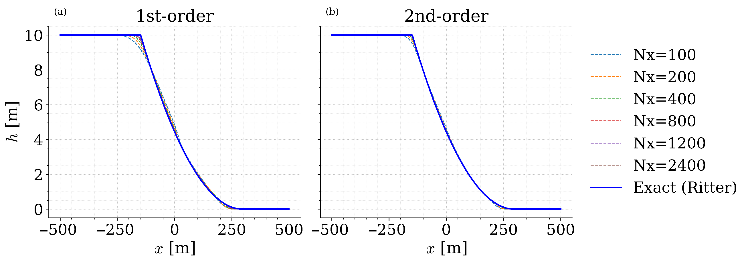
Figure A2.
Comparison between the numerical and Ritter analytical solutions for the unit discharge at s. Panel (a) shows the first-order solution, while panel (b) shows the second-order solution.
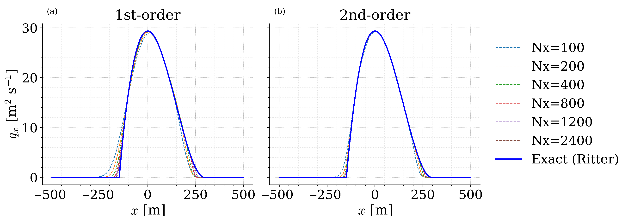
Figure A3.
Comparison between the numerical and Ritter analytical solutions for the velocity profile at s. Panel (a) shows the first-order solution, while panel (b) shows the second-order solution.
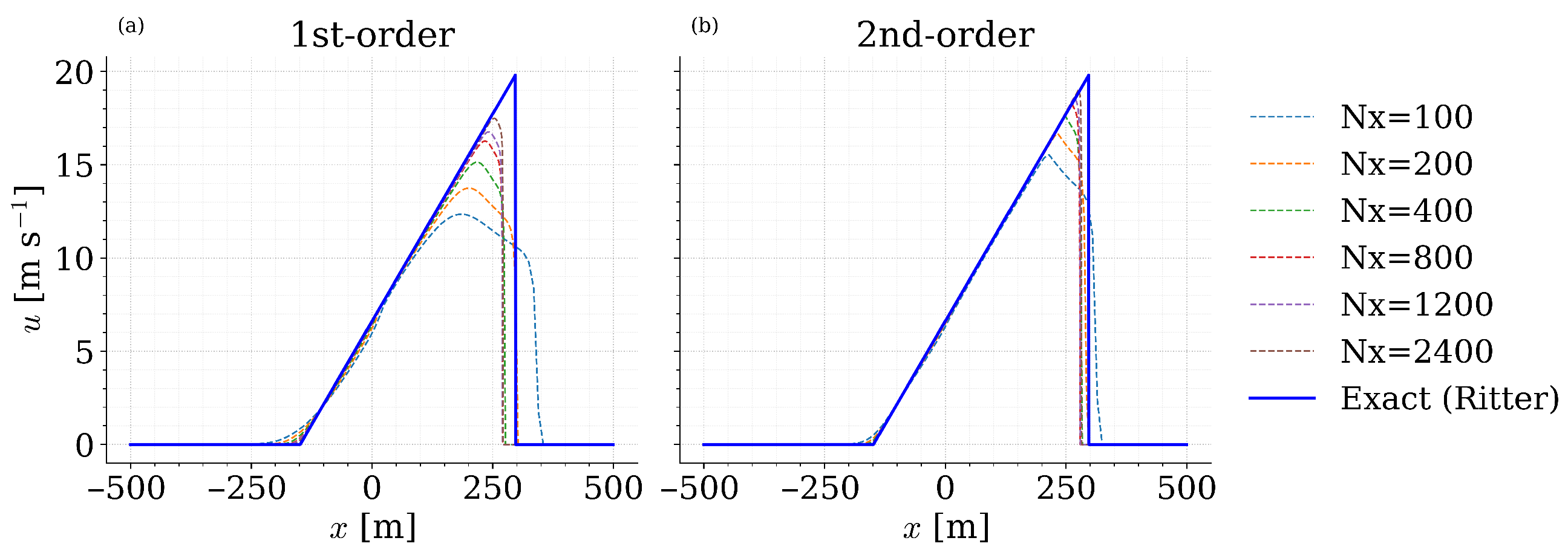
Table A1.
errors for the Ritter dam-break test at s for the first-order (O1) and second-order (O2) HLLC schemes.
Appendix A.2.2. Lake at Rest
A second validation test was performed to verify the well-balanced property of the numerical solver. The objective of this benchmark is to assess whether the scheme is able to preserve an exact stationary equilibrium in the presence of non-uniform topography, without generating spurious oscillations in either free-surface elevation or velocity.
The test consists of a quiescent water layer over a non-flat bed. In the present case, the bottom topography is defined as the superposition of a planar slope and a smooth local bump, so that the bed elevation varies in both horizontal directions. The initial condition is prescribed by imposing a constant free-surface elevation
with zero initial velocity,
The initial thickness is therefore obtained from
In exact arithmetic, this configuration should remain steady for all times. Therefore, any departure from the initial state is purely numerical and provides a direct measure of the well-balanced quality of the discretization. In the present implementation, this property relies on the combination of hydrostatic reconstruction and consistent source-term treatment through the Audusse-type flux splitting [9].
The test was carried out on a 2D domain of size m and m, discretized with and . The maximum bed elevation is used to define the constant free-surface level m, ensuring that the entire domain remains wet. Two numerical configurations were considered: a first-order scheme in space and time, and a second-order scheme in space and time. The simulation was run up to s.
Figure A4a shows the final longitudinal free-surface profile, with an inset around the equilibrium level. The zoom reveals that both numerical solutions remain in agreement with the exact equilibrium up to machine precision, confirming that the solver preserves the stationary state over non-flat topography without spurious oscillations.
This result is further confirmed in Figure A4b, where the final free-surface error
is shown along the same section. The profile is identically zero, within floating-point roundoff, for both numerical configurations. This demonstrates that no measurable imbalance is introduced by the bed-slope source term discretization.
A quantitative summary is reported in Table A2. For both simulation orders, the final errors are exactly zero in the stored diagnostics, and the maximum residual velocity remains below m/s. These results confirm that the implemented solver is exactly well-balanced for the lake-at-rest equilibrium on non-uniform topography.
Figure A4.
(a) Midline section of the free-surface elevation for the lake-at-rest test at the final time, with a zoomed inset around the equilibrium level. (b) Final midline error in free-surface elevation, , for the lake-at-rest test.
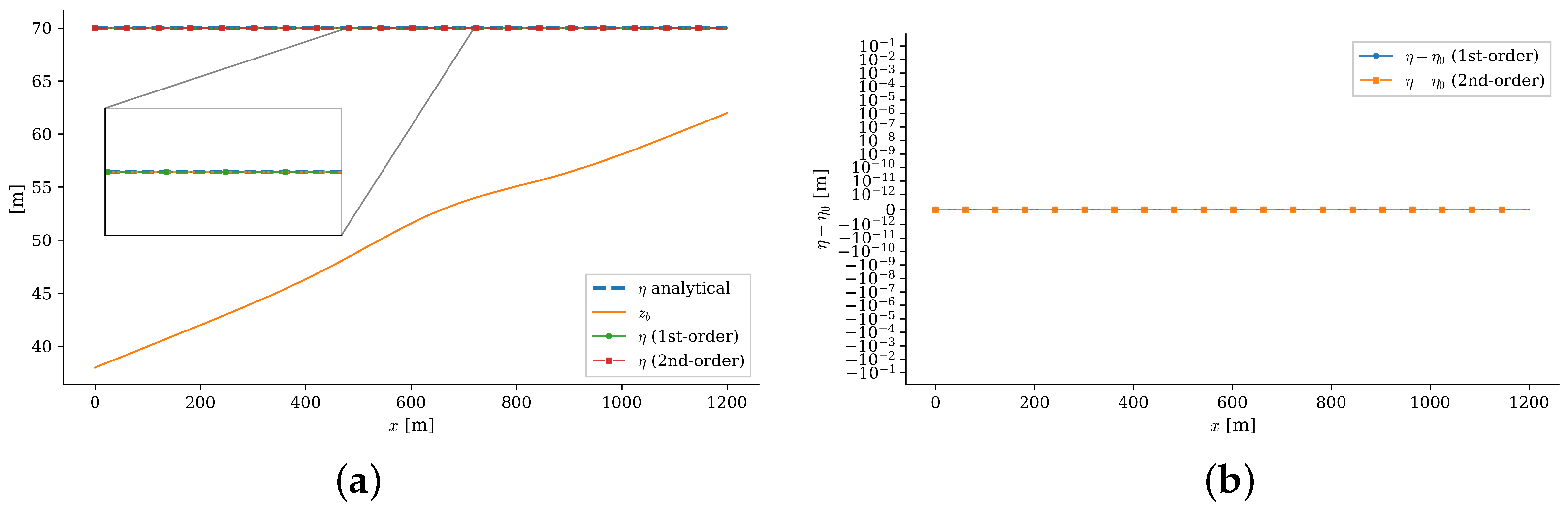
Table A2.
Summary metrics for the lake-at-rest test for the first-order and second-order HLLC schemes.
Appendix A.2.3. Grid and Time-Step Convergence
An additional verification test was performed to evaluate the sensitivity of the numerical solution to spatial and temporal discretization. The analysis focuses on a diagnostic quantity defined as the flow thickness at a prescribed control point inside the computational domain.
The test is performed on a synthetic 2D topography composed of a planar slope combined with a smooth Gaussian bump. The initial condition corresponds to a fully wet configuration with constant free-surface elevation , perturbed by a small Gaussian disturbance. The initial flow thickness is therefore defined as
where denotes the bed elevation. The free surface is initialized as
with perturbation amplitude m. The initial momentum components are set to zero everywhere.
The simulation is integrated up to s using the second-order numerical configuration (MUSCL spatial reconstruction combined with SSPRK2 time integration). To evaluate convergence properties, the value of the thickness is extracted at a control point located at fixed fractional coordinates within the domain. To reduce sensitivity to the exact grid alignment, the diagnostic value is computed as the maximum thickness within a small local window surrounding the target point.
Spatial Convergence
Spatial convergence was assessed by refining the computational grid while keeping the time step effectively controlled by the CFL condition. The user-defined time step was therefore set to a very large value so that the actual time step is determined exclusively by the stability constraint.
The grid sequence considered in this study is
Figure A5a shows the variation of as a function of the grid spacing . The value of the monitored quantity decreases slightly with increasing resolution and tends toward a stable value as the mesh is refined. The corresponding absolute errors, computed with respect to the finest grid solution, are shown in Figure A6a. The corresponding numerical values of and for each grid resolution are also reported in Table A3. The error decreases consistently as the grid is refined, indicating convergence of the numerical solution.
Temporal Convergence
Temporal convergence was evaluated by fixing the spatial grid at cells and varying the user-defined time step over the sequence
The resulting values of are shown in Figure A5b. The diagnostic quantity remains almost constant across the tested time steps, with only very small variations for larger . The corresponding absolute errors, computed relative to the smallest time step, are reported in Figure A6b. The numerical values of the tested time steps and the associated monitored thicknesses are summarized in Table A4. The error decreases as the time step is reduced, confirming the expected temporal convergence of the scheme.
Overall, the results indicate that the solver exhibits stable and consistent behaviour with respect to both spatial and temporal refinement. The variations in the monitored quantity remain small and decrease monotonically as the discretization is refined, confirming the robustness of the implemented numerical method.
Figure A5.
Monitored thickness as a function of discretization parameters: (a) versus spatial resolution ; (b) versus time step .
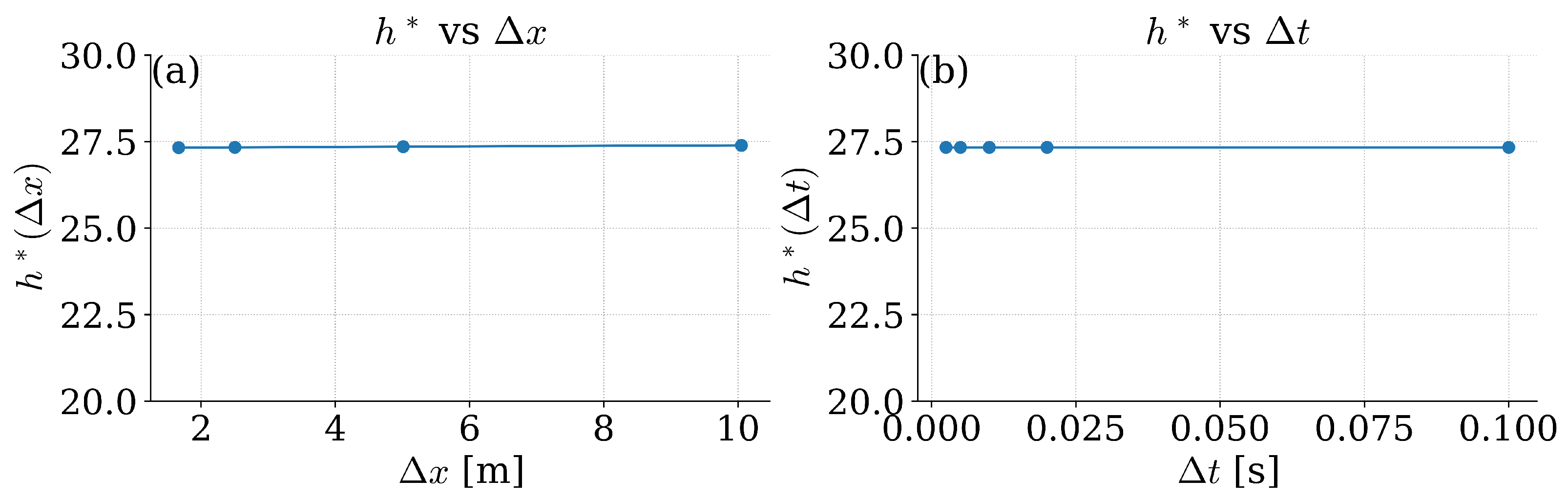
Figure A6.
Absolute error in the monitored thickness : (a) error relative to the finest spatial resolution; (b) error relative to the smallest time step.
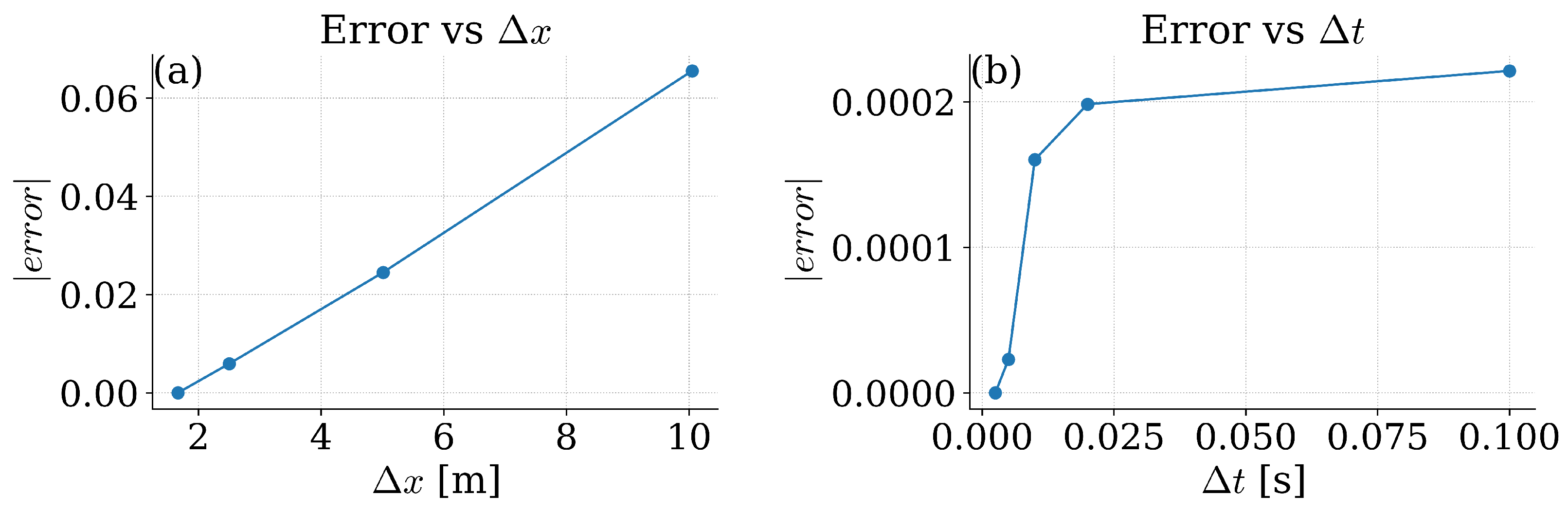
Table A3.
Spatial convergence results for the monitored quantity .
Table A4.
Temporal convergence results for the monitored quantity .
Appendix A.2.4. Mass Conservation
The conservation of mass was assessed through a dedicated numerical test on a flat bed, without inflow, friction, erosion, or any additional source term. Under these conditions, the total mass should remain constant in time, so that any variation can be attributed exclusively to numerical errors.
The initial condition consists of a smooth 2D hump of flow thickness centred in the computational domain,
with zero initial momentum and flat topography,
The total mass is computed at each output time as
and compared with the initial mass . The corresponding relative mass error is defined as
where is a small positive number introduced only to avoid division by zero in degenerate cases.
The test was performed on a domain of size m and m, discretized with and , and integrated up to s. Two numerical configurations were considered: the first-order scheme in space and time and the second-order scheme in space and time.
Figure A7 shows the relative mass error on a logarithmic scale. Panel (a) corresponds to the first-order scheme and panel (b) to the second-order one. The first-order scheme reaches a maximum relative error of and a final relative error of . The second-order scheme shows slightly larger but still very small deviations, with a maximum relative error of and a final relative error of .
These values are extremely small and confirm that the implemented solver remains effectively conservative in practice. The slightly larger drift observed for the second-order scheme is consistent with the use of reconstructed interface states, SSPRK2 time integration, and positivity corrections, which may introduce roundoff-level cumulative effects. However, the overall error remains below throughout the simulation, which is fully acceptable for the intended applications.
A quantitative summary is reported in Table A5. In both cases, the absolute mass variation remains several orders of magnitude smaller than the total initial mass, confirming that the conservative structure of the numerical flux formulation is correctly preserved.
Figure A7.
Relative mass error as a function of time for the two numerical schemes: (a) first-order scheme, (b) second-order scheme.
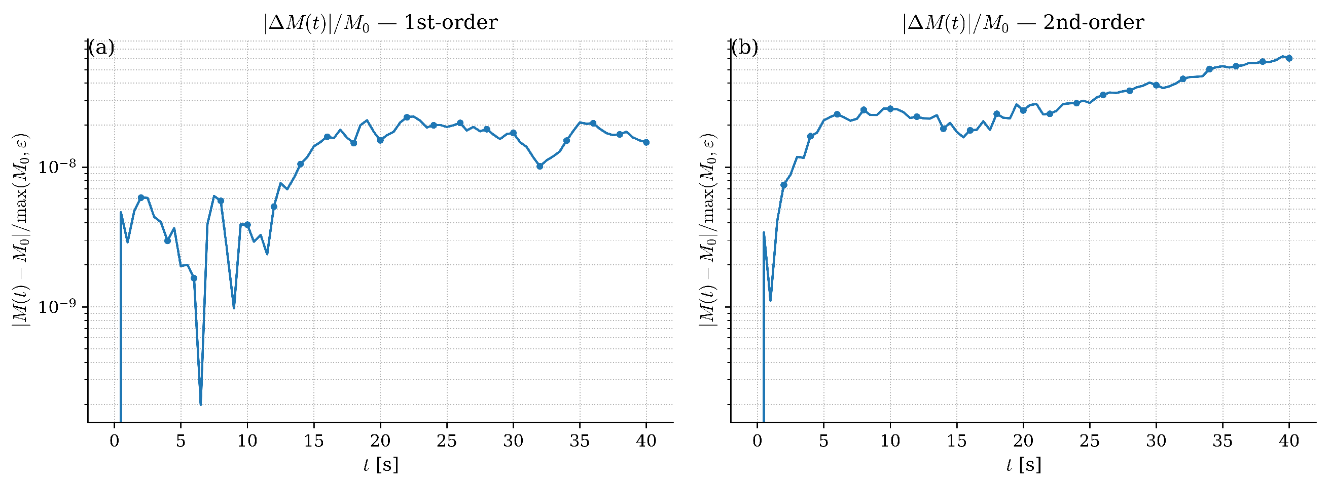
Table A5.
Summary metrics for the mass-conservation test for the first-order (O1) and second-order (O2) schemes.
Appendix A.3. Validation on Real Cases
Appendix A.3.1. Validation on the Morino–Rendinara Real Case
As a real-case application, the proposed numerical model was tested against the Morino–Rendinara debris-flow event discussed by Pasculli et al. [6]. The reference study presents a back-analysis of the Rio Sonno debris-flow channel using the RAMMS software, providing quantitative information on the expected magnitude of the flow in terms of maximum velocity and final accumulation height.
For the present comparison, the same general scenario was reproduced by adopting a released debris volume of , a material density of , and a DEM with spatial resolution of . The rheological setting was defined consistently with the real Morino–Rendinara case, using two spatially variable dry-friction coefficients, and , together with a turbulent friction parameter . The simulation was performed on the real topography of the Morino area using the HLLC-based shallow-flow solver with second-order spatial reconstruction, second-order SSPRK time integration, and hybrid local fallback to first–order near critical wet–dry or strongly discontinuous regions. The corresponding thresholds were four times the dry-depth threshold for minimum depth, with , when the free-surface jump exceeded , or when the local velocity exceeded .
The rheological formulation was based on a Voellmy-type law, with spatially variable friction regions introduced to account for different channel and fan behaviours. The release area and computational window were selected interactively on the real DEM in order to reproduce the documented flow path and depositional sector.
Figure A8a shows the final flow thickness at . These numerical results were compared with the values reported in the reference RAMMS back-analysis Figure A8b. In particular, [6] reports a peak flow velocity of approximately and a maximum flow-front height at the channel outlet of about . In the present simulation, the global maximum velocity was found to be , reached at , whereas the final maximum flow height was , evaluated at .
Overall, the simulated values are in good agreement with the published reference ranges. The computed peak velocity is slightly larger than the reference RAMMS value, but still falls within the prescribed acceptance interval adopted for validation. The final maximum thickness is also fully consistent with the range expected from the published back-analysis. Therefore, the Morino test can be considered successfully reproduced by the proposed solver.
Table A6.
Comparison between the present simulation and the reference values reported for the Morino–Rendinara case.
Figure A8.
Validation for the Morino–Rendinara real case: (a) final flow-height distribution obtained with the present numerical model at ; (b) reference deposition map reported in the RAMMS back-analysis by Pasculli et al. [6].
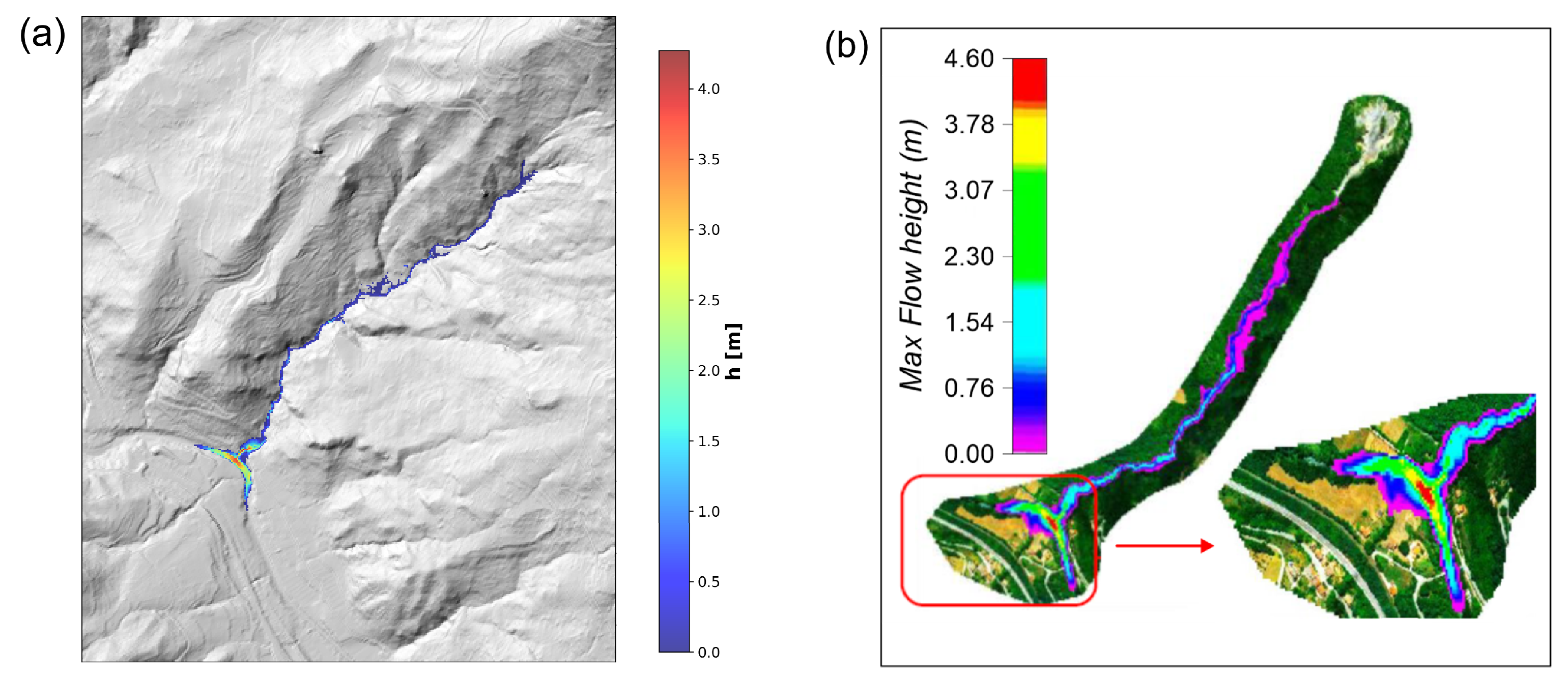
Appendix A.3.2. Validation on the Marsicano–Pescasseroli Real Case
A second real-case validation was performed using the debris-flow scenario described in the Marsicano–Pescasseroli study reported in [60]. The purpose of this test is to evaluate the capability of the proposed shallow-flow solver to reproduce large-scale debris-flow propagation on real topography.
The simulation uses the same numerical solver presented in the previous sections, based on the HLLC Riemann solver with hydrostatic reconstruction and positivity preservation. In this configuration, second-order spatial discretization and second-order time integration were adopted, combined with the hybrid stabilization strategy that locally activates a more robust formulation near wet–dry transitions or strong surface gradients. The corresponding thresholds were twenty-five times the dry-depth threshold for minimum depth, with , for the free-surface jump, or for velocity.
The computational domain was extracted from the regional DEM covering the Marsicano area. The original DEM was resampled to a spatial resolution of , consistent with the resolution used in the reference study. After clipping the region of interest, the resulting computational grid consists of and cells. The debris release was defined through an interactive polygon representing the source area described in the reference study. The total released volume was , which was distributed uniformly within the release polygon at the initial time. The rheological behaviour was described using a Voellmy-type friction law with parameters , , and a material density of . The simulation was performed for a total physical time of [60].
Figure A9a compares the final flow-height distribution at with the reference map reported in the literature Figure A9b [60].
The numerical results were compared with the reference values reported in the Marsicano study. In the present simulation, the global maximum velocity was found to be , reached at . The final maximum flow thickness was , evaluated at the end of the simulation.
A qualitative comparison between the two final flow-height maps shows a good agreement in terms of overall runout pattern, lateral spreading, and preferential accumulation in the depositional area at the valley outlet. In particular, both maps highlight the formation of the main depositional lobe in the downstream fan area, where the largest thickness values are concentrated. Minor differences can be observed in the detailed shape of the depositional margins and in the local spatial distribution of thickness, which may reasonably be attributed to differences in numerical treatment, topographic preprocessing, or graphical post-processing. Nevertheless, the overall agreement confirms that the proposed model is able to reproduce the main propagation and deposition features of the Marsicano real case.
Table A7.
Comparison between the present simulation and the reference values reported for the Marsicano case.
Figure A9.
Validation for the Marsicano–Pescasseroli real case: (a) final flow-height distribution obtained with the present numerical model at ; (b) reference deposition map reported in the literature by Paglia et al. [60].
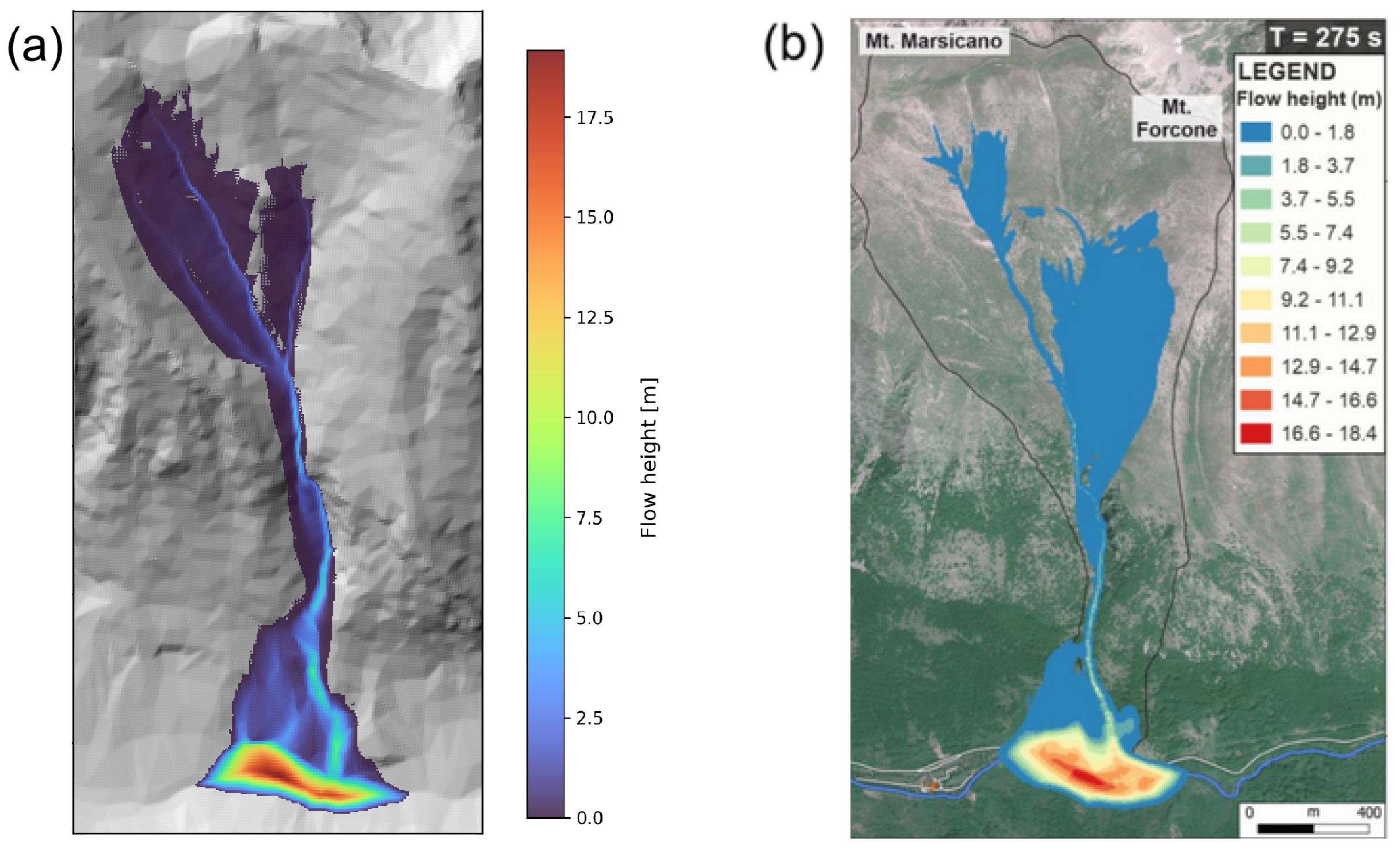
Appendix A.4. Detailed Formulation of the Training Loss
The training objective adopted in this work is a masked multi-component mean squared error designed to account for the padded structure of the dataset and for the different physical relevance of depth and velocity variables. Let denote the predicted output tensor, the corresponding target, and let be the validity mask identifying the valid spatio-temporal support of each sample.
In addition, active-flow cells are identified through the indicator
where
For the flow-thickness field, a weighted masked mean squared error is introduced in order to assign greater importance to active-flow regions while still accounting for dry cells. The local weighting function is defined as
with
Accordingly, the thickness loss is written as
For the velocity components, the loss is evaluated only over active-flow cells, so as to avoid penalizing predictions in dry regions where velocity is physically negligible or undefined. The corresponding masked mean squared errors are
and
The total loss used during training is therefore given by
References
- Alcántara-Ayala, I. Landslides in a changing world. Landslides 2025, 22, 2851–2865. [Google Scholar] [CrossRef] [Scilit]
- Miccadei, E.; Carabella, C.; Paglia, G. Landslide Hazard and Environment Risk Assessment. Land 2022, 11, 428. [Google Scholar] [CrossRef] [Scilit]
- Iverson, R.M. The Physics of Debris Flows. Rev. Geophys. 1997, 35, 245–296. [Google Scholar] [CrossRef] [Scilit]
- Arattano, M.; Franzi, L. Influence of Rheology on Debris-Flow Dynamics. Nat. Hazards Earth Syst. Sci. 2006. [Google Scholar] [CrossRef] [Scilit]
- Pasculli, A.; Cinosi, J.; Turconi, P.; Sciarra, N. Learning Case Study of a Shallow-Water Model to Assess an Early-Warning System for Fast Alpine Muddy-Debris-Flow. Water 2021, 13, 750. [Google Scholar] [CrossRef] [Scilit]
- Pasculli, A.; Zito, C.; Sciarra, N.; Mangifesta, M. Back Analysis of a Real Debris Flow, the Morino–Rendinara Test Case (Italy), Using RAMMS Software. Land 2024, 13, 2078. [Google Scholar] [CrossRef] [Scilit]
- Chung, T.J. Computational Fluid Dynamics, 4th ed.; Cambridge University Press: Cambridge, UK, 2006; p. 1012. [Google Scholar]
- Pasculli, A. Viscosity variability impact on 2D laminar and turbulent Poiseuille velocity profiles; characteristic-based split (CBS) stabilization. In Proceedings of the 2018 5th International Conference on Mathematics and Computers in Sciences and Industry (MCSI), Corfu, Greece, 25–27 August 2018; pp. 770–771. [Google Scholar]
- Audusse, E.; Bouchut, F.; Bristeau, M.-O.; Klein, R.; Perthame, B. A fast and stable well-balanced scheme with hydrostatic reconstruction for shallow water flows. SIAM J. Sci. Comput. 2004, 25, 2050–2065. [Google Scholar] [CrossRef] [Scilit]
- Gallouët, T.; Hérard, J.-M.; Seguin, N. Some approximate Godunov schemes to compute shallow-water equations with source terms. Comput. Fluids 2003, 32, 479–513. [Google Scholar] [CrossRef] [Scilit]
- Murillo, C.J.J.; Garcia-Navarro, P. 2D simulation of granular flow over irregular steep slopes using global and local coordinates. J. Comput. Phys. 2013, 255, 166–204. [Google Scholar] [CrossRef] [Scilit]
- Zienkiewicz, O.C.; Taylor, R.L. The Finite Element Method for Solid and Structural Mechanics, 6th ed.; Elsevier: London, UK, 2006; p. 631. [Google Scholar]
- Paik, J. A high resolution finite volume model for 1D debris flow. J. Hydro-Environ. Res. 2015, 9, 145–155. [Google Scholar] [CrossRef] [Scilit]
- Pasculli, A.; Minatti, L.; Sciarra, N.; Paris, E. SPH modeling of fast muddy debris flow: Numerical and experimental comparison of certain commonly utilized approaches. Ital. J. Geosci. 2013, 132, 350–365. [Google Scholar] [CrossRef] [Scilit]
- Pastor, M.; Haddad, B.; Sorbino, G.; Cuomo, S.; Drempetic, V. A depth integrated coupled SPH model for flow-like landslides and related phenomena. Int. J. Numer. Anal. Methods Geomech. 2009, 33, 143–172. [Google Scholar] [CrossRef] [Scilit]
- Del Pin, F.; Aubry, R. The particle finite element method: An overview. Int. J. Comput. Methods 2004, 1, 267–307. [Google Scholar] [CrossRef] [Scilit]
- Idelsohn, S.R.; Oñate, E.; Del Pin, F. The particle finite element method: A powerful tool to solve incompressible flows with free-surfaces and breaking waves. Int. J. Numer. Meth. Eng. 2004, 61, 964–989. [Google Scholar] [CrossRef] [Scilit]
- Bouchut, F. Nonlinear Stability of Finite Volume Methods for Hyperbolic Conservation Laws; Springer: Berlin/Heidelberg, Germany, 2004. [Google Scholar]
- Toro, E.F. Riemann Solvers and Numerical Methods for Fluid Dynamics, 3rd ed.; Springer: Berlin/Heidelberg, Germany, 2009. [Google Scholar]
- Christen, M.; Kowalski, J.; Bartelt, P. RAMMS. Numerical simulation of dense snow avalanches in three-dimensional terrain. Cold Reg. Sci. Technol. 2010, 63, 1–14. [Google Scholar] [CrossRef] [Scilit]
- Hungr, O.; McDougall, S. Two numerical models for landslide dynamic analysis. Comput. Geosci. 2009, 35, 978–992. [Google Scholar] [CrossRef] [Scilit]
- Mergili, M.; Fischer, J.T.; Krenn, J.; Pudasaini, S.P. r.avaflow v1, an advanced open-source computational framework for the propagation and interaction of two-phase mass flows. Geosci. Model. Dev. 2017, 10, 553–569. [Google Scholar] [CrossRef] [Scilit]
- Pitman, E.B.; Nichita, C.C.; Patra, A.; Bauer, A.; Sheridan, M.; Bursik, M. Computing granular avalanches and landslides. Phys. Fluids 2013, 15, 3638–3646. [Google Scholar] [CrossRef] [Scilit]
- Dash, R.K.; Kanungo, D.P.; Malet, J.P. Runout modelling and hazard assessment of Tangni debris flow in Garhwal Himalayas, India. Environ. Earth Sci. 2021, 80, 338. [Google Scholar] [CrossRef] [Scilit]
- Ullah, I.; Shafique, M.; Ali Khattak, G.; Shah, A. Debris flow simulations for hazard, vulnerability and risk assessment in the Karkorum mountain ranges, northern Pakistan. Remote Sens. Appl. Soc. Environ. 2024, 36, 101329. [Google Scholar]
- Audisio, C.; Pasculli, A.; Sciarra, N. Conceptual and numerical models applied on the River Pellice (North Western Italy). In Engineering Geology for Society and Territory, Volume 3: River Basins, Reservoir Sedimentation and Water Resources; Springer International Publishing: Cham, Switzerland, 2015; pp. 327–330. [Google Scholar]
- Cesca, M.; D’Agostino, V. Comparison Between FLO-2D and RAMMS in Debris-Flow Modelling: A Case Study in the Dolomites. WIT Trans. Eng. Sci. 2008, 60, 197–206. [Google Scholar]
- Schraml, K.; Thomschitz, B.; McArdell, B.W.; Graf, C.; Kaitna, R. Modeling Debris-Flow Runout Patterns on Two Alpine Fans with Different Dynamic Simulation Models. Nat. Hazards Earth Syst. Sci. 2015, 15, 1483–1492. [Google Scholar] [CrossRef] [Scilit]
- Mikoš, M.; Bezak, N. Debris Flow Modelling Using RAMMS Model in the Alpine Environment with Focus on the Model Parameters and Main Characteristics. Front. Earth Sci. 2021, 8, 605061. [Google Scholar] [CrossRef] [Scilit]
- FLO-2D Europe. Condizioni di Vendita e Politica di Rinnovo della Licenza Software FLO-2D PRO. Available online: https://www.flo-2deurope.com (accessed on 30 March 2026).
- WSL Institute for Snow and Avalanche Research SLF. RAMMS::Debrisflow Licensing and Shop Information. Available online: https://ramms.ch (accessed on 30 March 2026).
- Hungr Geotechnical Inc. DAN3D Order and License Types. Available online: https://hungr-geotech.com (accessed on 30 March 2026).
- Lu, L.; Jin, P.; Karniadakis, G.E. Learning Nonlinear Operators via DeepONet. Nat. Mach. Intell. 2021, 3, 218–229. [Google Scholar] [CrossRef] [Scilit]
- Bihlo, A.; Popovych, R.O. Physics-informed neural networks for the shallow-water equations on the sphere. J. Comput. Phys. 2022, 456, 111024. [Google Scholar] [CrossRef] [Scilit]
- Nag, P.; Zammit-Mangion, A.; Singh, S.; Cressie, N. Spatio-temporal modeling and forecasting with Fourier neural operators. arXiv 2026, arXiv:2601.01813. [Google Scholar] [CrossRef] [Scilit]
- Yang, Q.; Hernandez-Garcia, A.; Harder, P.; Ramesh, V.; Sattigeri, P.; Szwarcman, D.; Watson, C.D.; Rolnick, D. Fourier neural operators for arbitrary resolution climate data downscaling. J. Mach. Learn. Res. 2024, 25, 1–30. [Google Scholar]
- Pasculli, A.; Secchi, M.; Mangifesta, M.; Cencetti, C.; Sciarra, N. A Novel Probabilistic Approach for Debris Flow Accumulation Volume Prediction Using Bayesian Neural Networks with Synthetic and Real-World Data. Geosciences 2025, 15, 362. [Google Scholar] [CrossRef] [Scilit]
- Li, Z.; Kovachki, N.; Azizzadenesheli, K.; Liu, B.; Bhattacharya, K.; Stuart, A.; An kumar, A. Fourier Neural Operator for Parametric PDEs. In Proceedings of the International Conference on Learning Representations (ICLR), Vienna, Austria, 4 May 2021. [Google Scholar]
- Tran, A.; Mathews, A.; Xie, L.; Ong, C.S. Fourier Neural Operator: A Generalist Neural Operator. arXiv 2022, arXiv:2202.09417. [Google Scholar]
- Kovachki, N.; Li, Z.; Liu, B.; Azizzadenesheli, K.; Bhattacharya, K.; Stuart, A.; An kumar, A. Neural Operator: Learning Maps Between Function Spaces. J. Mach. Learn. Res. 2023, 24, 1–97. [Google Scholar]
- Secchi, M.; Pasculli, A.; Mangifesta, M.; Sciarra, N. Learning Debris Flow Dynamics with a Deep Learning Approach. Geosciences 2026, 16, 55. [Google Scholar] [CrossRef] [Scilit]
- Voellmy, A. Über die Zerstörungskraft von Lawinen. Schweiz. Bauztg. 1955, 73, 159–165. [Google Scholar]
- Partheniades, E. Erosion and Deposition of Cohesive Soils. J. Hydraul. Div. 1965, 91, 105–139. [Google Scholar] [CrossRef] [Scilit]
- Pasculli, A.; Sciarra, N. A Probabilistic Approach to Determine the Local Erosion of a Watery Debris Flow. In Proceedings of the XI IAEG International Congress, Liege, Belgium, 3–8 September 2006; p. S08-08, ISBN 978-296006440-7. [Google Scholar]
- Murphy, A.H. Skill Scores Based on the Mean Square Error and Their Relationships to the Correlation Coefficient. Mon. Weather Rev. 1988, 116, 2417–2424. [Google Scholar] [CrossRef] [Scilit]
- Reich, N.G.; Parajuli, R.R.; Sweitzer, M.D.; Lauer, S.A.; Iamsirithaworn, S.; Shrestha, S. Case Study in Evaluating Time Series Prediction Models Using the Relative Mean Absolute Error. Am. Stat. 2016, 70, 286–292. [Google Scholar] [CrossRef] [Scilit]
- Gladstone, R.J.; Rahmani, H.; Suryakumar, V.; Meidani, H.; D’Elia, M.; Zareei, A. Mesh-based GNN surrogates for time-independent PDEs. Sci. Rep. 2024, 14, 3394. [Google Scholar] [CrossRef] [Scilit]
- Cho, S.W.; Lee, J.Y.; Hwang, H.J. Learning time-dependent PDE via graph neural networks and deep operator network for robust accuracy on irregular grids. J. Comput. Phys. 2026, 544, 114430. [Google Scholar] [CrossRef] [Scilit]
- Li, Z.; Kovachki, N.; Azizzadenesheli, K.; Liu, B.; Bhattacharya, K.; Stuart, A.; Anandkumar, A. Neural Operator: Graph Kernel Network for Partial Differential Equations. arXiv 2020, arXiv:2003.03485. [Google Scholar] [CrossRef] [Scilit]
- Wu, H.; Luo, H.; Wang, H.; Wang, J.; Long, M. Transolver: A Fast Transformer Solver for PDEs on General Geometries. In Proceedings of the 41st International Conference on Machine Learning; PMLR: Cambridge, MA, USA, 2024. [Google Scholar]
- Raissi, M.; Perdikaris, P.; Karniadakis, G.E. Physics-informed neural networks: A deep learning framework for solving forward and inverse problems involving nonlinear partial differential equations. J. Comput. Phys. 2019, 378, 686–707. [Google Scholar] [CrossRef] [Scilit]
- Li, Z.; Zheng, H.; Kovachki, N.; Jin, D.; Chen, H.; Liu, B.; Azizzadenesheli, K.; Anandkumar, A. Physics-Informed Neural Operator for Learning Partial Differential Equations. ACM/IMS J. Data Sci. 2024, 1, 9. [Google Scholar] [CrossRef] [Scilit]
- McClenny, L.; Braga-Neto, U. Self-Adaptive Physics-Informed Neural Networks using a Soft Attention Mechanism. J. Comput. Phys. 2023, 474, 111722. [Google Scholar] [CrossRef] [Scilit]
- Jagtap, A.D.; Kharazmi, E.; Karniadakis, G.E. Conservative Physics-Informed Neural Networks on Discrete Domains for Conservation Laws: Applications to Forward and Inverse Problems. Comput. Methods Appl. Mech. Eng. 2020, 365, 113028. [Google Scholar] [CrossRef] [Scilit]
- Trenta, A.; Cossu, A.; Bacciu, D. Learning and Transferring Physical Models through Derivatives. Trans. Mach. Learn. Res. 2026. Available online: https://openreview.net/forum?id=IbBCDDeDF7 (accessed on 25 February 2026).
- Trenta, A.; Cossu, A.; Bacciu, D. ComPhy: Composing Physical Models with end-to-end Alignment. In Proceedings of the International Conference on Learning Representations (ICLR); Available online: https://openreview.net/forum?id=ER7zDJXtRI (accessed on 25 February 2026).
- Rusanov, V.V. Calculation of Interaction of Non-Steady Shock Waves with Obstacles. USSR Comput. Math. Math. Phys. 1961, 1, 304–320. [Google Scholar] [CrossRef] [Scilit]
- Ritter, A. Die Fortpflanzung der Wasserwellen. Z. Ver. Dtsch. Ingenieure 1892, 36, 947–954. [Google Scholar]
- Willmott, C.J.; Matsuura, K. Advantages of the Mean Absolute Error (MAE) over the Root Mean Square Error (RMSE) in Assessing Average Model Performance. Clim. Res. 2005, 30, 79–82. [Google Scholar] [CrossRef] [Scilit]
- Paglia, G.; Santucci, G.; Buccolini, M.; Miccadei, E. Assessment of Potential Landslide Scenarios Using Morphometry, Geomorphological Constraints, and Run-Out Analysis: A Case Study from Central Apennines (Italy). Land 2025, 14, 2109. [Google Scholar] [CrossRef] [Scilit]
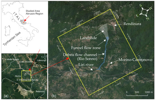
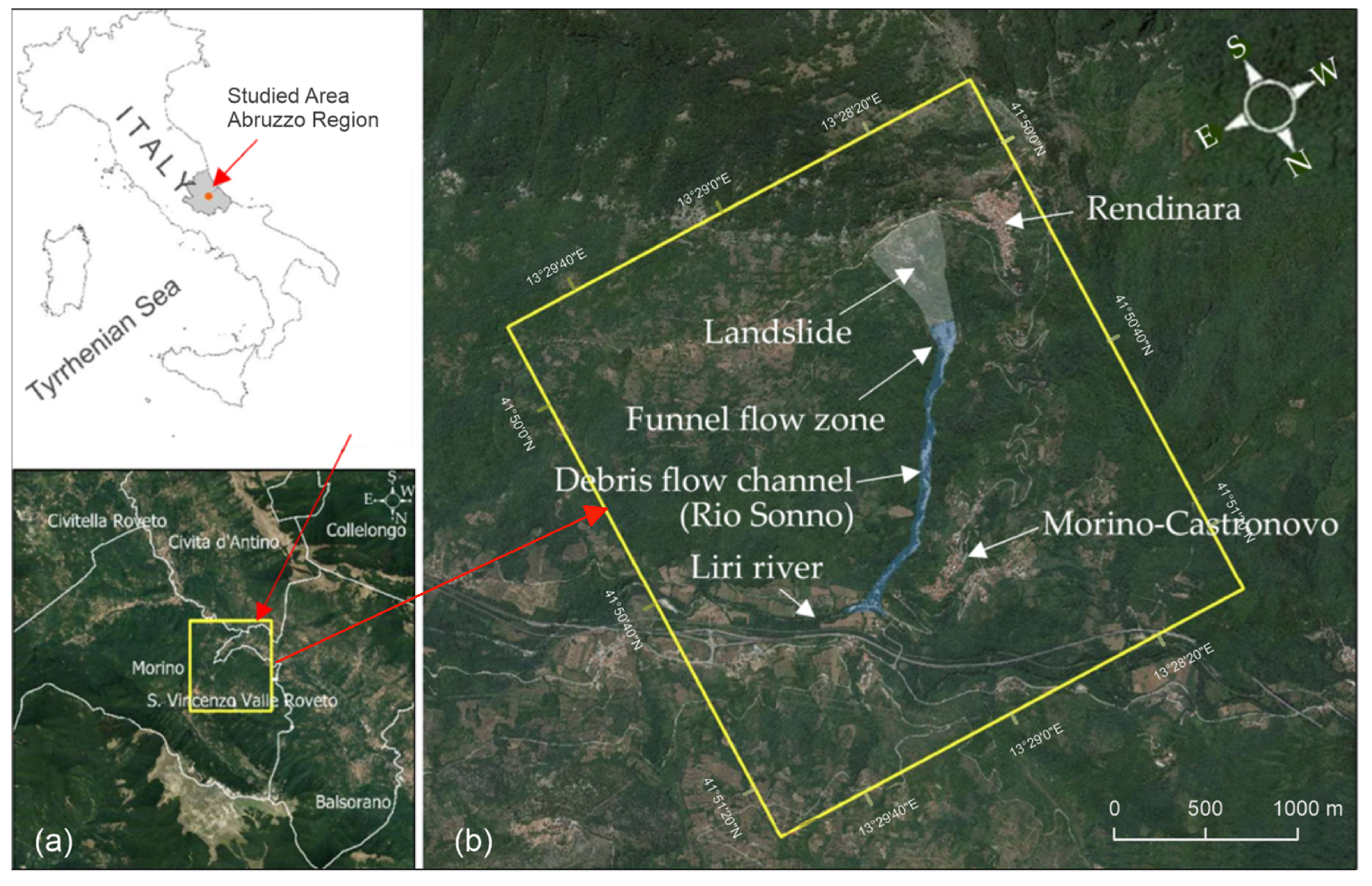
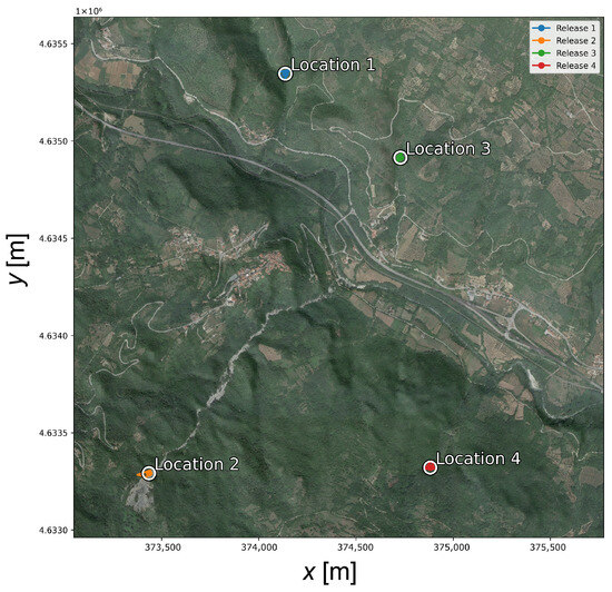
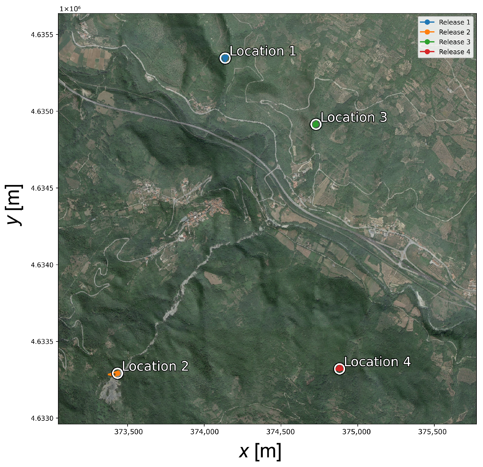
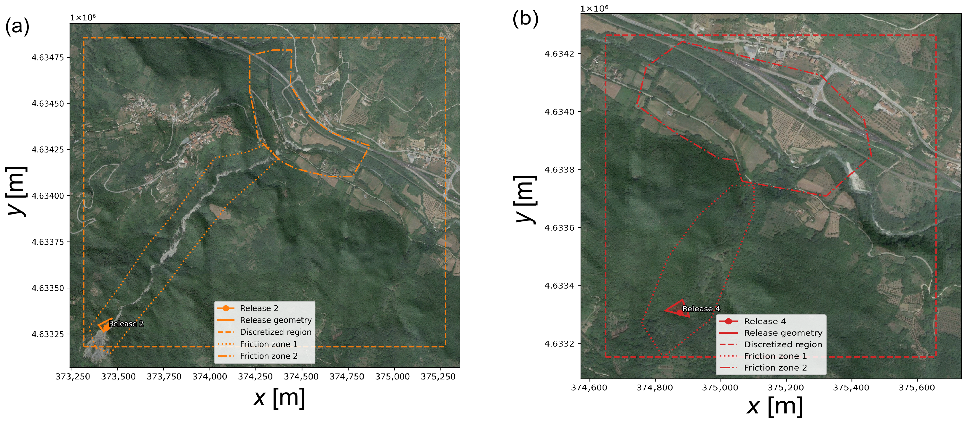
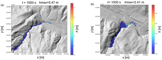
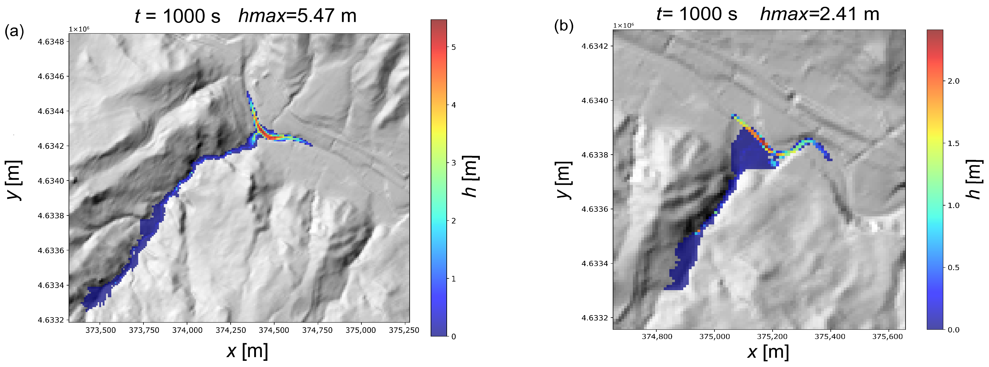
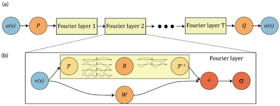
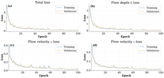
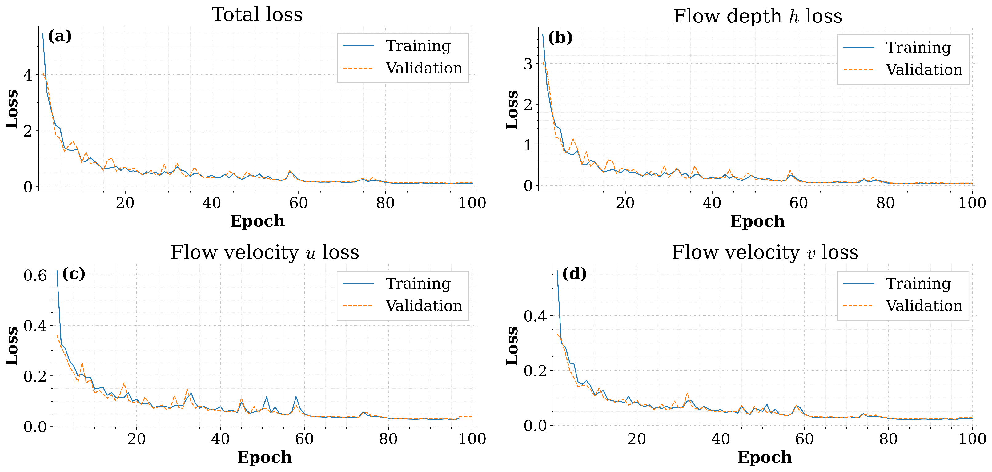
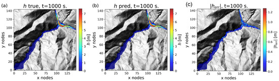
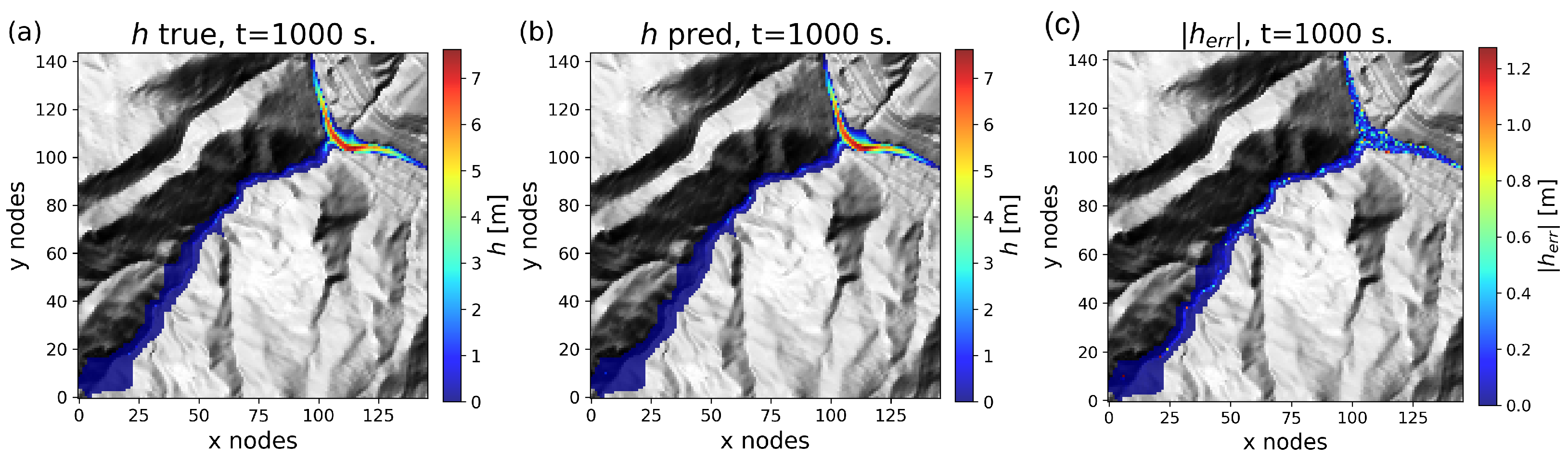
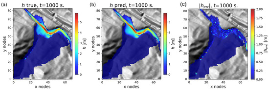
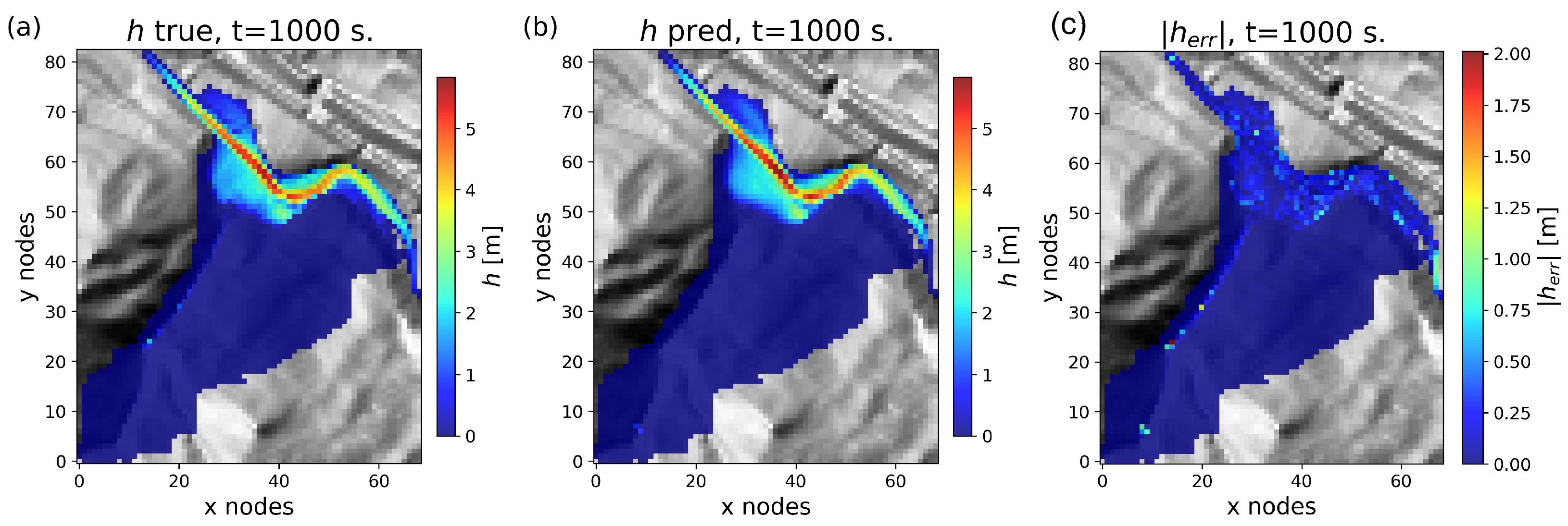
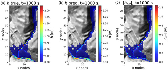
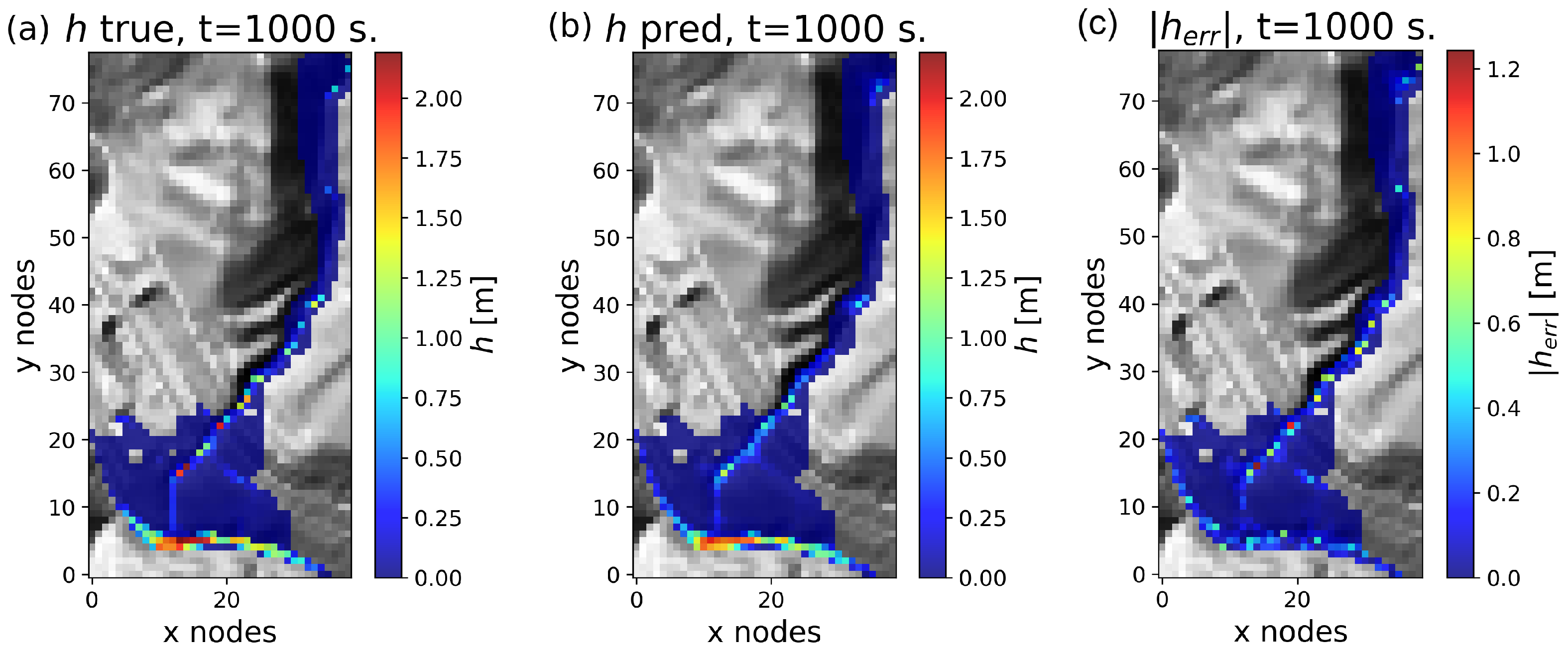
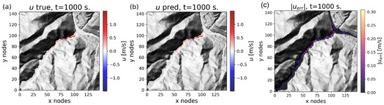
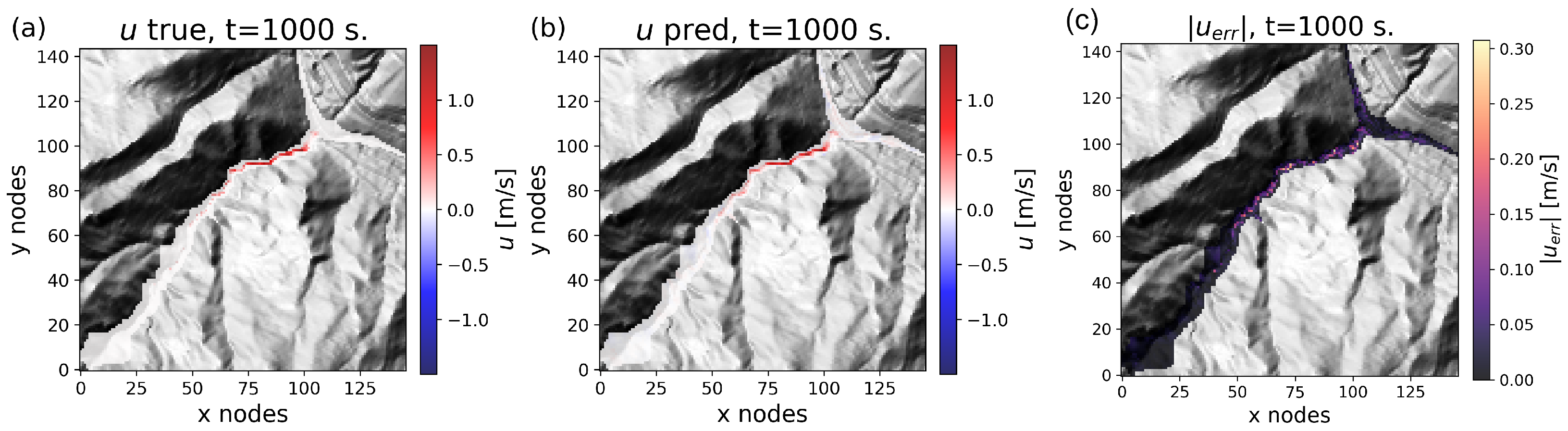
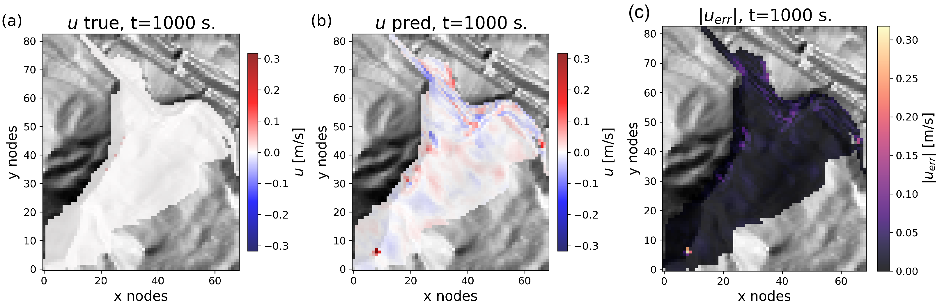
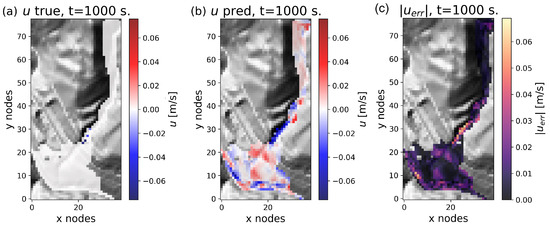
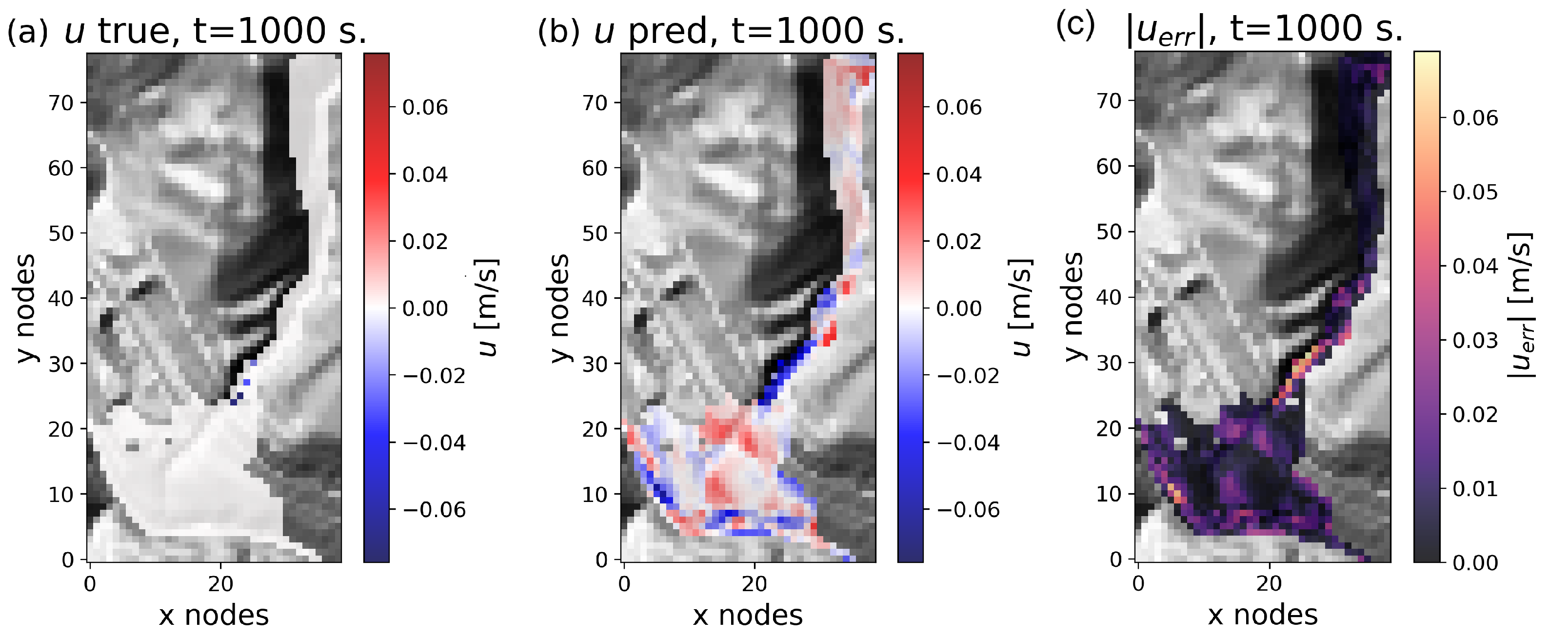
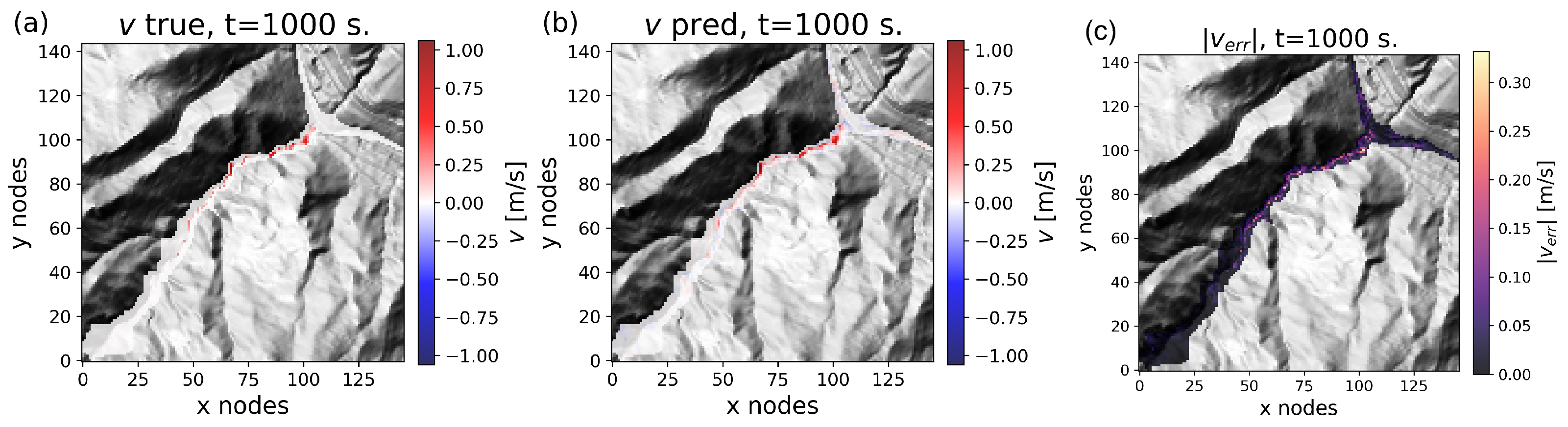
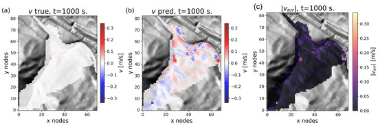
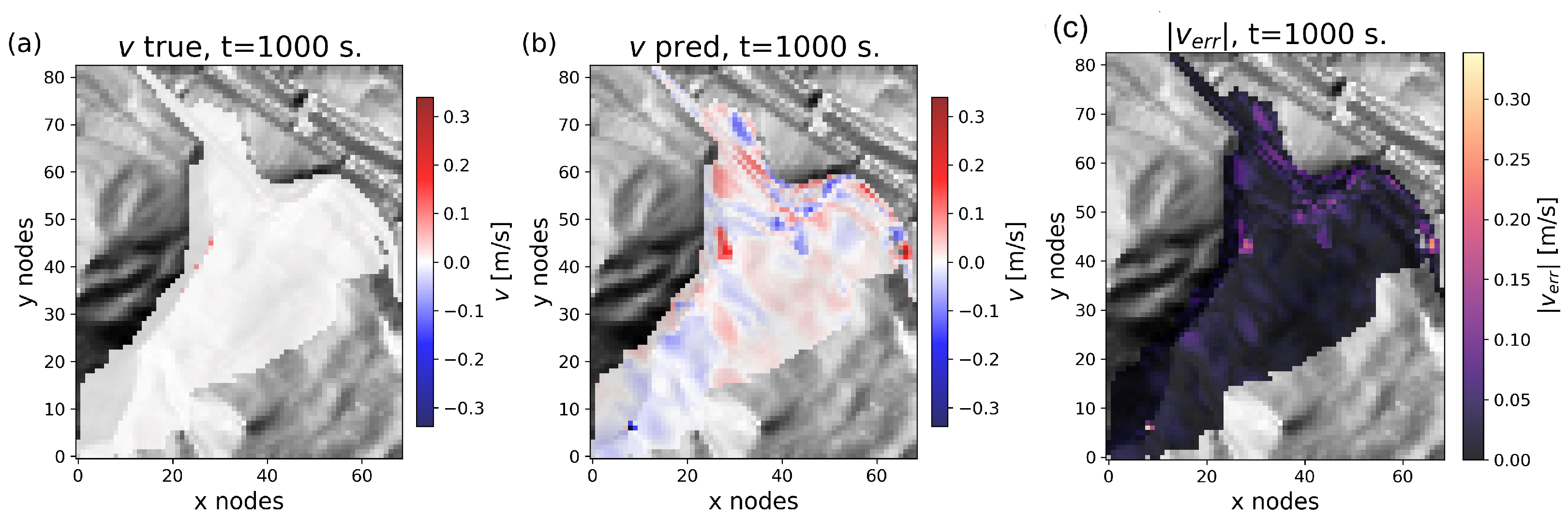
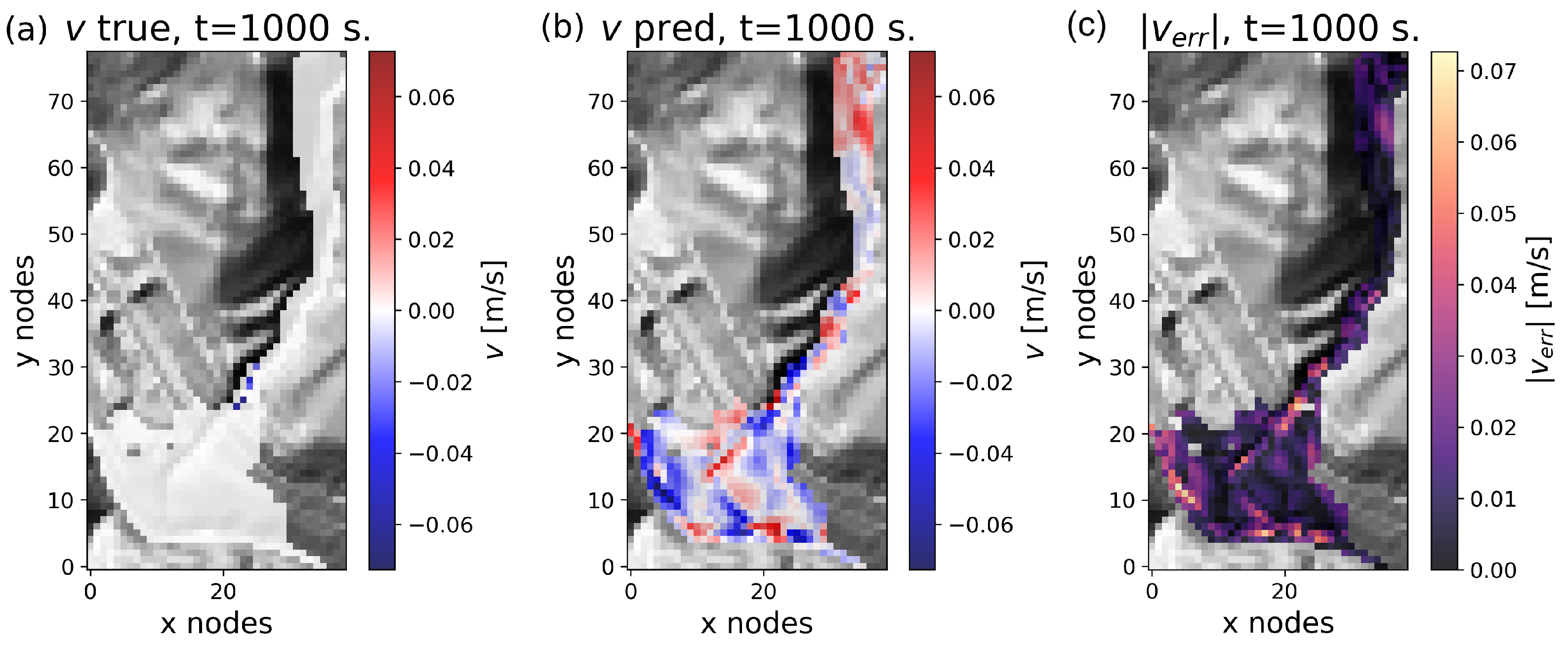

Disclaimer/Publisher’s Note: The statements, opinions and data contained in all publications are solely those of the individual author(s) and contributor(s) and not of MDPI and/or the editor(s). MDPI and/or the editor(s) disclaim responsibility for any injury to people or property resulting from any ideas, methods, instructions or products referred to in the content. |
© 2026 by the authors. Licensee MDPI, Basel, Switzerland. This article is an open access article distributed under the terms and conditions of the Creative Commons Attribution (CC BY) license.