


Abstract
Coastal ecosystems are highly dynamic and vulnerable to climate change, sea-level rise, and rapid urbanization. However, many landscape ecological risk assessments are limited by fixed scales and assumptions of spatial uniformity. This study develops a geomorphology-based framework to analyze coastal ecological risk. Using multi-source data from 1980 to 2020, the optimal analytical scale was identified as 120 m (grain) and 1000 m (extent). An integrated approach combining OPGD, XGBoost–SHAP, and restricted cubic spline (RCS) models was applied to examine risk patterns and driving mechanisms across four coastal types in Guangdong, China. The results show that the importance and interactions of driving factors vary significantly among geomorphic types, with clear nonlinear responses. Key statistical thresholds were identified, indicating ranges where risk sensitivity changes, including NDVI ≈ 0.624 in the Hilly Ria Coast, slope ≈ 2.8° in the Platform Ria Coast, elevation ≈ 14.5 m in the Barrier–Lagoon Coast, and GDP ≈ 1644.65 × 106 CNY/km2 in the Estuarine Delta Coast. These findings provide quantitative evidence for understanding spatial heterogeneity and the nonlinear dynamics of coastal ecological risk, and offer practical references for adaptive management.
1. Introduction
Coastal zones, shaped by intense land–sea interactions, support diverse ecosystems—from mangroves and salt marshes to coastal wetlands—while delivering critical ecosystem services and space for economic development [1,2]. Yet climate change, sea-level rise, and accelerating human activities are rapidly degrading these systems. Habitat loss, landscape fragmentation, and biodiversity decline have made many coastal regions among the most vulnerable on Earth [3,4]. These pressures create growing uncertainty and underscore the need for adaptive management strategies capable of responding to dynamic environmental change. In this context, satellite remote sensing has emerged as a powerful tool for long-term monitoring, enabling continuous tracking of land-use dynamics and landscape pattern evolution in coastal areas.
Landscape ecological risk assessment (LERA) quantifies the potential ecological impacts of landscape pattern change [5] and serves as a widely used diagnostic and early-warning tool for regional ecological security [6]. Rooted in the pattern–process–risk paradigm, LERA links land-use change to ecosystem vulnerability and potential damage within coupled human–natural systems [7]. Recent studies have extended the framework through spatial risk mapping [8,9], driver analysis [10,11], scenario simulations [12,13], integration with ecosystem services [5,14], and management zoning [15,16], underscoring its growing role in spatial planning and environmental decision-making.
At the core of LERA lies the landscape ecological risk index (LERI), which integrates land-use change with landscape configuration [17]. Although scale calibration and grid-based GIS analysis are standard, LERA outcomes remain highly sensitive to spatial scale, making identification of an optimal analytical scale essential for reliable results [18,19]. Researchers have explored spatial heterogeneity using geographical detectors and geographically weighted regression [20], and process-oriented models (e.g., minimal cumulative resistance and gravity models) to examine risk propagation [21]. To date, most applications have targeted mountainous regions [22,23], urban agglomerations [19,24], and watersheds [25,26], revealing strong spatial dependence among risk drivers. Coastal zones have only recently gained attention, with early work on framework development [27,28], pattern characterization [29], and driving-factor analysis [30]. However, their use in supporting adaptive coastal management remains limited.
However, existing studies still show notable limitations in process understanding, management relevance, and regional specificity, which constrain both theoretical development and practical application. (1) Limited understanding of driving processes. Landscape ecological processes are inherently complex and nonlinear, yet most studies rely on linear or generalized linear models. As a result, interactions among multiple drivers and potential threshold responses are not well captured. Although nonlinear effects have been observed in coastal systems, such as port expansion and aquaculture impacts [31,32,33], these processes have not been systematically interpreted within a landscape ecological risk framework. In addition, machine learning models (e.g., GBM) often function as “black boxes” [11], limiting their ability to explain drivers and identify critical thresholds. (2) Weak linkage to management. Identifying response thresholds is essential for linking risk assessment to spatial management. While threshold effects and regime shifts have been widely discussed [34,35], most studies focus on mountainous and urban regions [23,30]. Applications in coastal systems remain limited, which restricts the practical relevance of current research. (3) Homogenized regional perspective. Many studies treat coastal zones as homogeneous units, overlooking strong geomorphological heterogeneity. Differences in landforms lead to distinct ecological processes and human disturbance patterns. Ignoring these differences may obscure the mechanisms of risk formation and reduce the spatial applicability of results.
To address the above limitations, this study focuses on two main contributions. First, a comparative analysis is conducted from a geomorphological perspective. Geomorphology provides the fundamental framework for natural differentiation in coastal zones. It controls sedimentary processes, hydrological conditions, and ecosystem types, and also shapes the spatial distribution and intensity of human activities. In this study, geomorphic stratification is introduced to link geomorphological units with risk characteristics. This approach allows the spatial heterogeneity of risk formation to be better captured and provides a physical basis for differentiated management. Second, an integrated analytical framework is developed, combining the optimal parameter-based geographical detector (OPGD) model, the XGBoost–SHAP framework, and the restricted cubic spline (RCS) model. This framework enables the interpretation of spatial differentiation, the quantification of nonlinear driver effects, and the identification of statistical thresholds. It allows the driving processes and threshold responses of landscape ecological risk to be systematically examined across different geomorphic types.
The proposed framework is applied to the mainland coastal zone of Guangdong Province, China, a rapidly urbanizing region that possesses the longest coastline in the country (4114.3 km). Using long-term satellite-derived land-use data and multi-source environmental datasets from 1980 to 2020, this study investigates the evolution of coastal ecological risk under sustained anthropogenic pressure. Guangdong encompasses diverse geomorphic settings, including the Hilly Ria Coast, Platform Ria Coast, Barrier–Lagoon Coast, and Estuarine Delta Coast [36]. The combination of complex geomorphology and intense socioeconomic development makes Guangdong an ideal case for examining how coastal ecological risk evolves under long-term human disturbance [37]. Because ria coasts, barrier–lagoon systems, and deltaic plains occur worldwide, the geomorphic stratification approach and threshold-based analytical framework developed in this study are transferable to other rapidly developing coastal regions facing similar tensions between economic growth and ecological conservation.
This study aims to integrate geomorphological comparison with an analytical framework to achieve three objectives. (1) A land-use classification system adapted to coastal characteristics is developed. The optimal spatial scale for landscape ecological risk assessment is identified. The spatiotemporal patterns of coastal landscape ecological risk from 1980 to 2020, as well as their variations across geomorphic types, are then revealed. (2) The integrated OPGD–XGBoost–SHAP–RCS framework is applied to identify key drivers of risk formation across different geomorphic types. Nonlinear effects are quantified, and response thresholds are identified. (3) Based on differences in driving processes and threshold responses, targeted management strategies are proposed for different coastal types. These findings provide scientific support for refined spatial planning, ecological restoration, and risk management in coastal zones.
2. Study Area and Materials
2.1. Study Area
Guangdong Province is located in southern mainland China (20°13′–25°31′ N, 109°39′–117°24′ E) and has China’s longest mainland coastline (4114.3 km). Tectonic processes and land–sea interactions have formed four major coastal geomorphic types: Hilly Ria Coast, Platform Ria Coast, Barrier–Lagoon Coast, and Estuarine Delta Coast (Figure 1) [37]. Rapid economic growth since China’s reform and opening-up has intensified differences in land use among these geomorphic settings, increasing spatial heterogeneity in coastal landscape ecological risk.
In this study, the coastal land zone is defined using the official “mean high tide line” released by the Ministry of Natural Resources as the land–sea boundary. Based on the national coastal zone and tidal flat resource survey standards (1980–1985) [38], the study area is further extended 10 km inland from this boundary. This definition follows established practice in coastal resource management in China and ensures consistency with previous studies. The focus of this study is on land-based processes driven by land use and human activities. Therefore, the marine area is not included as a separate analytical unit.
Previous studies have shown that human activities in coastal zones are mainly concentrated within nearshore land areas [39,40]. A 10 km inland extent is sufficient to capture major disturbance sources, including urban expansion, agricultural development, and infrastructure construction. This spatial extent is intended to capture land-dominated processes rather than the full influence of marine dynamics, such as storm surges or sea-level rise. Accordingly, the variable “distance to the seaside” reflects the gradient of proximity to the coast in relation to land-based activities, rather than a complete land–sea coupling process.
Figure 1.
Location of the study area. (a) Geographic location of Guangdong Province within China; (b) mainland coastal zone of Guangdong Province, classified into four coastal types [41]; (c) Hilly Ria Coast, represented by Dapeng Bay in Shenzhen; (d) Platform Ria Coast, represented by Liusha Bay in Zhanjiang; (e) Barrier–Lagoon Coast, represented by Jieshi Bay in Shanwei; (f) Estuarine Delta Coast, represented by the Pearl River Estuary in Guangzhou. The base map in panel (a) is derived from the Standard Map Service of the Ministry of Natural Resources of China (review number GS (2019) 1652; http://bzdt.ch.mnr.gov.cn/).
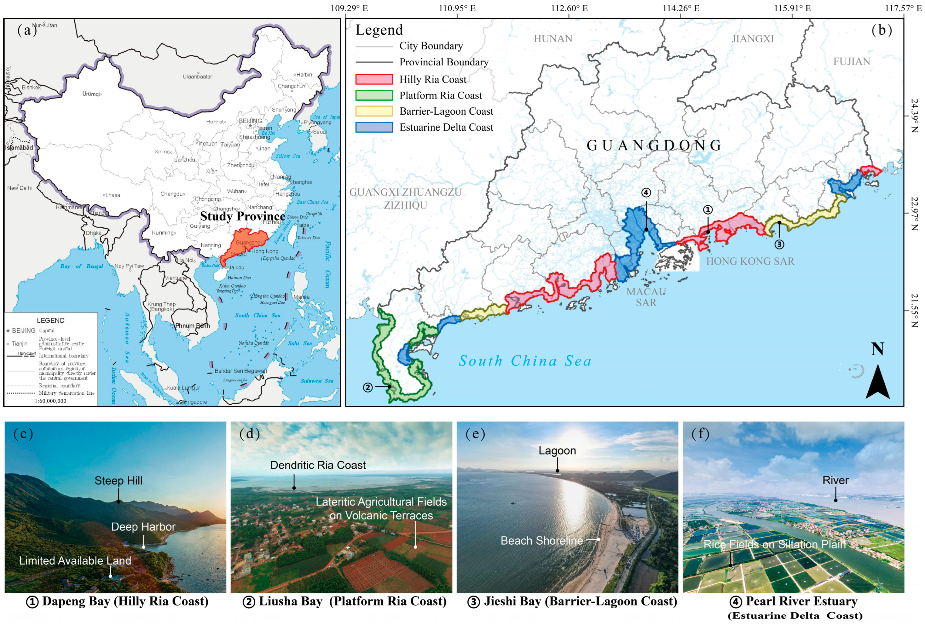
The spatial classification of coastal geomorphic types in this study is derived from authoritative regional records, including the Guangdong Provincial Gazetteer: Ocean and Islands [38]. It represents a spatial translation and application of existing classification schemes rather than the development of a new system. Specifically, the spatial extents of different geomorphic types reported in the literature were digitized and matched with the study area using GIS. The classification was further validated through visual interpretation of remote sensing imagery in representative regions. Based on this process, the study area was divided into four typical coastal types, with their key characteristics and spatial distributions described as follows:
- (1)
- Hilly Ria Coast. Steep bedrock terrain and limited sediment supply restrict the availability of land for development, though deep-water harbors are common. This type extends from the eastern Pearl River Estuary to Honghai Bay and from the western estuary to Hailing Bay, including Zhelin Bay.
- (2)
- Platform Ria Coast. Formed on a volcanic platform incised by drowned dendritic valleys, well suited for deep-water port development. Limited freshwater availability constrains agriculture, and local livelihoods depend mainly on port operations and fisheries. It is concentrated around the Leizhou Peninsula.
- (3)
- Barrier–Lagoon Coast. Consisting of sand barriers, sandbars, and semi-enclosed lagoons, this coast supports fisheries and salt production but is prone to erosion due to its sandy substrates. It flanks the Hilly Ria Coast, extending from Haimen Bay to Honghai Bay in the east and from Hailing Bay to the Jianjiang River Estuary in the west.
- (4)
- Estuarine Delta Coast. Formed on alluvial plains with anastomosing channels, this coast is characterized by extensive reclaimed farmland and occurs mainly at major river mouths (e.g., the Pearl, Han, Rong, Lian, Jian, and Nandu rivers).
2.2. Study Period
Three time points (1980, 2000, and 2020) were selected to examine the long-term evolution of landscape ecological risk in coastal zones. This selection was based on the following considerations.
- (1)
- Representativeness of socioeconomic stages. The year 1980 marks the onset of China’s reform and opening-up policy and coastal development strategy. The years 2000 and 2020 correspond to key transitions associated with rapid urbanization and high-quality development, respectively. The two 20-year intervals capture major shifts in socioeconomic structures and spatial policies.
- (2)
- Data availability and comparability. These three time points ensure consistent and reliable data for 15 selected drivers. This provides a solid basis for multi-period comparison and integrated modeling.
- (3)
- Alignment with research objectives. The purpose of this design is to compare distinct development stages and identify major trends and dominant patterns of risk evolution. It is not intended to represent continuous dynamics or detect abrupt change points. Therefore, milestone-based time points were adopted for the analysis.
2.3. Data Sources and Processing
Multi-source geospatial datasets for 1980, 2000, and 2020 were compiled and subjected to uniform preprocessing as described below.
- (1)
- Land-use data
Land-use datasets for 1980, 2000, and 2020 were obtained from the National Geographic Conditions Monitoring Cloud Platform (www.dsac.cn). These datasets were produced using standardized remote sensing interpretation procedures, with an initial spatial resolution of 30 m. According to the official validation report, the overall accuracy is 86.5% (Kappa = 0.82). This level of accuracy meets the requirements for regional-scale landscape analysis in landscape ecology.
To better capture coastal human activities, the classification was refined by adding Aquaculture land and Salt pan following Pan et al. [41]. The original classes were reclassified in ArcGIS Pro 3.5.3 into eight categories (Table 1). USGS satellite imagery (earthexplorer.usgs.gov) was used for auxiliary validation.
Table 1.
Reclassification of land use types and related descriptions.
- (2)
- Driver data
A total of 15 driving factors were selected in this study. Their data sources, formats, and processing methods are listed in Table 2. To ensure temporal comparability, all variables were constructed for the three time points (1980, 2000, and 2020).
Table 2.
List of driving factors for landscape ecological risk analysis.
To integrate multi-source data with different spatial resolutions, a unified spatial processing framework was established. All datasets were projected to a common coordinate system and aligned to the same spatial extent. Given the differences in original resolutions (e.g., NDVI at 250 m, population and GDP at 1000 m), direct resampling to a single grid was avoided to reduce potential bias. Instead, a point-based extraction approach using a unified analysis unit was applied. Specifically, rectangular grids derived from the optimal extent analysis were used as basic evaluation units. The centroid of each grid cell was generated as a common sampling location for all variables. For raster data, values were extracted directly from the original pixel at each centroid. For vector data (points, lines, and polygons), Euclidean distance rasters were first generated, and values were then extracted at the same centroid locations.
This approach avoids biases introduced by arbitrary resampling and ensures that all variables are spatially aligned to a consistent set of sampling points. It also reduces issues related to the modifiable areal unit problem (MAUP) and scale mismatch. Finally, all variables were normalized to eliminate differences in units and to ensure comparability for subsequent modeling.
3. Research Framework and Methods
3.1. Research Framework
Given the diversity of geomorphic types and the intensity of human activities in coastal zones, a hierarchical analytical framework was developed. This framework consists of three components: spatiotemporal pattern analysis, driving process diagnosis, and threshold response identification (Figure 2). It is designed to reveal the spatial–temporal patterns of landscape ecological risk, identify key driving processes, and detect potential response thresholds across different coastal types.
Figure 2.
Analytical framework for coastal landscape ecological risk based on “spatiotemporal pattern analysis—driving process diagnosis—threshold response identification”.
- (1)
- Spatiotemporal pattern analysis. This step aims to characterize the spatial patterns and temporal dynamics of ecological risk, providing a basis for subsequent analysis of driving processes. A reliable analysis requires a consistent spatial reference. Therefore, the optimal spatial grain and extent were first determined by integrating landscape metrics and geostatistical analysis. Based on these results, a uniform grid system was constructed as the basic evaluation unit. On this basis, the spatial clustering and temporal evolution of landscape ecological risk were examined across four coastal types. This step addresses where risk is concentrated and how it evolves over time.
- (2)
- Driving process diagnosis. To identify the factors shaping the spatial–temporal variation in risk, 15 potential drivers were selected from four dimensions: natural conditions, human activities, spatial proximity, and ecological regulation (Table 3). Two complementary methods were applied. The optimal parameter-based geographical detector (OPGD) model was used to quantify the explanatory power (q-statistic) of each factor for the spatial pattern of risk, as well as their interactions. The XGBoost–SHAP framework was used to evaluate the marginal contribution of each factor to local risk levels. By integrating the results from these two approaches, structural drivers shaping large-scale patterns were distinguished from process-related drivers influencing local risk variation. Key drivers were then selected for threshold analysis.
- (3)
- Threshold response identification. To translate nonlinear relationships into management-relevant insights, this step focuses on identifying critical thresholds in the relationship between drivers and ecological risk. For each key driver, a restricted cubic spline (RCS) model was fitted to capture its nonlinear relationship with landscape ecological risk (LERI). Thresholds were defined as points where the slope of the fitted curve changes markedly or where plateau regions begin. These thresholds represent statistically derived turning points that indicate changes in risk sensitivity. They provide quantitative references for spatial management. However, they should not be interpreted as strict ecological tipping points indicating abrupt system shifts.
Table 3.
Candidate drivers and their rationale.
3.2. Research Methods
3.2.1. Optimal Spatial Scale
Landscape metrics capture landscape configuration and are scale-dependent [42]. To identify an appropriate scale for coastal LERA, we optimized both grain size and spatial extent.
- (1)
- Optimal grain size
Land-use maps were resampled in ArcGIS Pro to ten grain sizes (30–300 m, 30 m interval). Following Ai et al. [18], 12 metrics (NP, PD, LPI, AREA_MN, SHAPE_AM, CONTAG, DIVISION, MESH, SPLIT, SHDI, SHEI, and AI; Table S1 in Supplementary Materials) were computed in FRAGSTATS 4.2. Information retention across grains was evaluated using the regional information loss index:
where is the relative area loss (%) of land-use type i; is the area (km2) after resampling; is the original area (km2); n is the number of land-use types; and S is the regional area-loss index. Larger S indicates greater information loss.
- (2)
- Optimal spatial extent
Based on the geostatistical “3 × grain” rule [43], eight grid extents (360–4000 m; Table S2 in Supplementary Materials) were generated in ArcGIS Pro using the fishnet tool. Each grid served as the analysis unit. Patch density (PD) and Shannon’s diversity index (SHDI) were selected because they are sensitive to extent and reflect fragmentation and heterogeneity, respectively. Spatial autocorrelation was assessed with the semivariogram:
Using the 2020 land-use map, semivariogram models for PD and SHDI were fitted in GS+ for each extent. The optimal extent was chosen based on model fit (R2) and the structured variance ratio.
3.2.2. Landscape Ecological Risk Model
Landscape ecological risk was quantified using a landscape ecological risk index (LERI), which integrates disturbance, vulnerability, and potential loss.
- (1)
- Landscape Disturbance Index (Ei)
Disturbance for land-use type i was computed from fragmentation (Ci), splitting (Ni), and dominance (Di):
Ci is the fragmentation index for landscape type i, reflecting the degree of patch fragmentation:
Ni is the splitting index for landscape type i, characterizing the spatial dispersion of its patches:
Di is the dominance index for landscape type i, indicating its dominant role in the overall landscape pattern:
Weights were set to a = 0.5, b = 0.3, and c = 0.2(a + b + c = 1) following Xu et al. [44] and coastal landscape characteristics.
- (2)
- Landscape Vulnerability Index (Fi)
Vulnerability reflects sensitivity and recovery difficulty under disturbance. Vulnerability ranks for the eight land-use types were assigned based on Ai et al. [18] and adjusted for coastal conditions (e.g., storm exposure, sea-level rise, development pressure) (Table S3 in Supplementary Materials). Values were normalized to [0, 1]:
- (3)
- Landscape Loss Index (Ri)
This index, determined by both disturbance and vulnerability, represents the degree of potential ecological loss for a specific landscape type:
- (4)
- Landscape Ecological Risk Index (LERI)
The study area was divided into N assessment units at the optimal scale. LERI for unit k was computed as the area-weighted mean of loss indices:
where is the area of type i in unit k, and Ak is total area of unit k. Larger LERI indicates higher ecological risk.
3.2.3. OPGD for Explaining Spatial Heterogeneity
To objectively identify the dominant drivers of spatial differentiation in coastal landscape ecological risk and their interactions, the optimal parameter-based geographical detector (OPGD) model was applied.
The OPGD model is an improved version of the traditional geographical detector. Its main advantage lies in the use of an embedded optimization algorithm to automatically determine the optimal discretization method (e.g., natural breaks and quantiles) and the number of classes for continuous variables. This approach reduces the bias introduced by subjective classification and improves the objectivity of spatial explanatory analysis [45].
The model analysis includes three modules [46]. (1) Parameter optimization: the optimal discretization scheme is identified for each driving factor. (2) Factor detection: the explanatory power of each individual factor on spatial risk differentiation is quantified. (3) Interaction detection: the combined effects of any two factors are evaluated to determine whether their interaction is independent, enhanced, or weakened.
Explanatory power was quantified using the q-statistic:
where N is the number of samples, L is the number of strata, σ2 is the overall variance of Y, and σh2 is the within-stratum variance. Higher q (0–1) indicates stronger explanatory power. Analyses were conducted in R 4.4.3 using the “GD” package.
3.2.4. XGBoost–SHAP for Predictive Contribution
To quantify the contributions of driving factors to LERI and capture nonlinear effects, the XGBoost model combined with the SHAP framework was applied. Unlike OPGD, which focuses on spatial differentiation, this approach evaluates factor contributions from a predictive perspective.
- (1)
- XGBoost model construction
XGBoost is a gradient boosting ensemble model that captures nonlinear relationships and interactions among variables [47]. It was implemented in Python 3.10 using the xgboost library. Key hyperparameters (e.g., max_depth, learning_rate, n_estimators, and subsample) were optimized using grid search with cross-validation.
- (2)
- SHAP-based interpretation
The SHAP framework was used to interpret model outputs based on Shapley values [41]. SHAP values quantify the marginal contribution of each factor. Global importance was assessed using mean absolute SHAP values, while the sign of SHAP values indicates whether a factor promotes or suppresses LERI. Summary and dependence plots were used to examine nonlinear response patterns.
- (3)
- Model training and evaluation
To account for spatial autocorrelation, spatial block cross-validation was applied instead of random splitting. The study area was divided into 1000 m blocks, with blocks alternately used for training and testing. Model performance was evaluated using MSE, RMSE, MAE, and R2.
The model is used to characterize nonlinear associations rather than to establish causal relationships. Results should therefore be interpreted as predictive associations.
3.2.5. Restricted Cubic Splines for Threshold Identification
To characterize nonlinear relationships between driving factors and LERI, restricted cubic spline (RCS) models were applied [23]. The RCS model fits smooth piecewise cubic functions by placing knots within the range of the independent variable, allowing nonlinear trends to be captured while maintaining continuity [48].
- (1)
- Model construction
The RCS model was implemented within a regression framework. Observed data points represent the relationship between each driver and LERI, while the fitted curve describes the smoothed response. To capture nonlinear structures, 3–5 knots were placed at selected quantiles (e.g., 5%, 50%, and 95%) of the predictor distribution.
- (2)
- Threshold identification
Thresholds were identified based on changes in the slope and curvature of the fitted curve. Specifically, they were defined as points where the slope changes markedly or inflection points occur. These values represent transitions in the sensitivity of LERI to changes in driving factors.
- (3)
- Uncertainty analysis
To assess robustness, a bootstrap procedure was applied. A total of 1000 resamples were generated with replacement. The RCS model was refitted for each sample, and thresholds were re-estimated. The empirical distribution of thresholds was used to derive 95% confidence intervals (CI), reflecting uncertainty in the estimates.
All analyses were conducted in R (version 4.4.3) using the “rms” package, with visualization performed using “ggplot2”.
4. Results
4.1. Analysis of Coastal Land Use Evolution
From 1980 to 2020, land use in Guangdong’s mainland coastal zone changed markedly. Both coast-wide trends and differences among geomorphic types reveal close associations between human activities and the coastal physical environment (Figure 3 and Figure 4).
Figure 3.
Land use classification results and corresponding area statistics for the Guangdong mainland coastal zone, 1980–2020.
Figure 4.
Land use area statistics for the four coastal types, 1980–2020.
4.1.1. Overall Trends (1980–2020)
The dominant trend was expansion of artificial land uses and contraction of natural and semi-natural cover. Construction land and aquaculture land increased the most, with net gains of 1555.68 km2 (+109.7%) and 1326.85 km2 (+433.1%), respectively. Farmland recorded the largest decline (−2520.16 km2). Bare land (e.g., tidal flats and marshes) and salt pans also decreased substantially (−32.7% and −57.7%), pointing to mounting pressure on coastal habitats. Forestland and water bodies remained relatively stable, with slight net increases. Overall, the coastal landscape shifted from predominantly agricultural and natural cover toward built-up and aquaculture land, driven mainly by urbanization and aquaculture expansion.
4.1.2. Differences Among Coastal Geomorphic Types
Hilly Ria Coast: Change was dominated by aquaculture expansion. Aquaculture land increased sharply (+726.8%), far outpacing construction land (+140.4%). This type recorded the largest aquaculture gain among the four coasts, consistent with its fishery-based economy and limited land available for development. Much of the expansion occurred through coastal reclamation.
Platform Ria Coast: Land use followed a “forest–farmland–settlement–sea” pattern. Forestland increased (+21.6%), making this the only type with a net forest gain. Aquaculture also expanded strongly (+512.5%), while construction land increased only slightly (+6.1%), indicating that land-use pressure was expressed mainly through production shifts rather than urban growth.
Barrier–Lagoon Coast: This type most closely mirrored the coast-wide trend but was distinguished by a redistribution of salt-pan activity. Overall changes were the smallest among the four types. Aquaculture and construction land increased, while farmland, forestland, and grassland declined slightly. Salt pans, concentrated on Barrier-Lagoon coasts in 1980, shifted in spatial concentration toward Platform Ria Coasts by 2000 and then declined sharply across the entire coast by 2020.
Estuarine Delta Coast: This type experienced the most intensive human disturbance and the most pronounced urbanization. Construction land grew rapidly (+204.0%), with a net increase exceeding 1000 km2. Farmland loss was also the greatest (−947.58 km2).
In sum, Guangdong’s coastal land use followed a shared trajectory toward construction and aquaculture, but the dominant pathway differed by geomorphic type: aquaculture-led expansion on Hilly Ria Coasts, concurrent forest and aquaculture gains on Platform Ria Coasts, salt-pan redistribution on Barrier–Lagoon Coasts, and rapid urbanization on Estuarine Delta Coasts. These contrasts provide context for interpreting the patterns and mechanisms of landscape ecological risk examined below.
4.2. Spatiotemporal Patterns of Coastal Landscape Ecological Risk
4.2.1. Risk Mapping at the Optimal Spatial Scale
- (1)
- Optimal grain size
To determine the optimal spatial grain for landscape ecological risk assessment, both landscape metric responses and area loss were analyzed. The results (Figure 5) show clear scale dependence of landscape metrics within the range of 30–300 m.
Figure 5.
Response curves of landscape indices to increasing grid (grain) size.
PD, NP, and SHDI varied strongly at grains below 120 m, indicating scale sensitivity and unstable metric responses (Figure 5). Several metrics (e.g., AREA_MN, AI, CONTAG) stabilized between 120 and 180 m, whereas grains above 180 m produced clear inflection points in multiple metrics (e.g., LPI, SHDI, SHEI), consistent with over-smoothing and information loss. Overall, based on the convergence behavior of multiple metrics, the optimal grain range was identified as 120–180 m.
To further validate the selection of optimal spatial grain, a landscape area loss model was applied (Figure 6). Information loss remained low (≤0.11%) below 120 m but rose rapidly at coarser grains, peaking at 0.6% for 240 m. At a grain size of 120 m, the loss index remains very low (approximately 0.06%) while meeting the principle of the coarsest acceptable resolution. This grain size achieves a balance between computational efficiency and information retention. Overall, considering both metric stability and information loss, 120 m was identified as the optimal spatial grain for landscape ecological risk assessment.
Figure 6.
Precision loss in landscape area under different grain sizes.
- (2)
- Optimal spatial extent
Based on the 2020 land-use data, the semivariogram fitting results of patch density (PD) and Shannon diversity index (SHDI) were evaluated across different spatial extents (Table 4 and Table 5). The optimal extent was determined by jointly considering spatial autocorrelation, model performance, and error control.
Table 4.
Changes in the semi-variogram of PD with varying spatial extents.
Table 5.
Changes in the semi-variogram of SHDI with varying spatial extents.
The results indicate that an extent of 1000 m achieves a balanced performance across these criteria. In terms of spatial autocorrelation, the nugget-to-sill ratios for PD and SHDI are 0.951 and 0.944, respectively, suggesting that spatial structure is still detectable and not dominated by random noise.
In terms of model performance, both metrics show high goodness-of-fit at this extent (PD: R2 = 0.988; SHDI: R2 = 0.983), indicating strong explanatory power. In addition, the residual sum of squares (RSS) is relatively low, and the range values (PD: 4350 m; SHDI: 4770 m) exceed four times the spatial grain, meeting geostatistical requirements.
- (3)
- Robustness and sensitivity of scale selection
To evaluate the sensitivity of scale selection across geomorphic types and the validity of using a unified scale, a robustness analysis was conducted. First, optimal scales were determined separately for each coastal type. The results (Tables S4–S11; Figures S1–S8 in Supplementary Materials) show that the Hilly Ria Coast has an optimal scale of 120 m (grain) and 1440 m (extent), the Platform Ria Coast 90 m and 1000 m, the Barrier–Lagoon Coast 120 m and 1000 m, and the Estuarine Delta Coast 120 m and 1440 m. These results indicate that the theoretically optimal scales vary across geomorphic types.
However, one objective of this study is to enable comparative analysis across different coastal types, which requires a consistent spatial framework. Therefore, results obtained under type-specific optimal scales were compared with those derived from a unified scale (120 m grain and 1000 m extent). The comparison shows that the relative differences in key landscape metrics (e.g., PD and SHDI) are less than 5%, and spatial patterns are highly consistent (Pearson’s r > 0.9) (Table S12 in Supplementary Materials).
These results suggest that, although optimal scales differ among coastal types, the unified scale captures the dominant spatial structures with high fidelity. Therefore, the use of a unified scale (120 m and 1000 m) is considered appropriate, and the main conclusions of this study are robust to scale selection.
- (4)
- Risk identification and classification
Based on the optimal spatial scale (120 m grain and 1000 m extent), land-use data were resampled and divided into 23,890 ecological risk assessment units in ArcGIS. These include 8306 units in the Hilly Ria Coast (34.77%), 6118 in the Platform Ria Coast (25.61%), 3648 in the Barrier–Lagoon Coast (15.27%), and 5818 in the Estuarine Delta Coast (24.35%). Landscape ecological risk values were calculated for each unit. Risk classification thresholds were determined using the natural breaks (Jenks) method based on the 2020 distribution and then consistently applied to 1980 and 2000 to ensure comparability. Five risk levels were defined: lowest (0–0.140), low (0.141–0.155), medium (0.156–0.166), high (0.167–0.176), and highest (0.177–0.230). The spatial distribution of landscape ecological risk for 1980, 2000, and 2020 is shown in Figure 7. This unified classification approach enables consistent comparison across time and avoids bias caused by varying classification standards.
Figure 7.
Spatial distribution of landscape ecological risk in the Guangdong mainland coastal zone from 1980 to 2020.
Landscape ecological risk reflects the combined effects of vulnerability and external pressure. To examine the sensitivity of key parameter settings, a sensitivity analysis was conducted for construction land, which is widely recognized as a critical and uncertain factor. Vulnerability values ranging from 2 to 4 were tested (Table S13; Figure S9 in Supplementary Materials). The results show that, although the mean LERI values vary slightly (<7%), spatial patterns remain highly consistent (pixel-level Pearson’s r > 0.97). Model error remains low (RMSE ≤ 0.014), and spatial autocorrelation patterns (Moran’s I) show no substantial change (r = 0.97–0.99).
These findings indicate that the main results, including spatial patterns and driving processes, are robust to variations in the vulnerability setting for construction land. This also suggests that assigning relatively low vulnerability to construction land does not lead to systematic underestimation of risk in highly urbanized areas, where risk is primarily driven by strong exposure and human pressure.
4.2.2. Spatial Clustering of Coastal Landscape Ecological Risk
To identify spatial clustering patterns of landscape ecological risk, a spatial weight matrix (W) was constructed at the 1000 m analysis unit scale. Global and local spatial autocorrelation analyses were then performed. A fixed distance band was used to define spatial neighbors, with units within 1000 m considered adjacent. Binary weights were applied and row-standardized to reduce the influence of varying neighbor counts. Global Moran’s I was calculated to assess overall spatial autocorrelation, and the Getis–Ord Gi* statistic was used to identify local hot spots (high-value clusters) and cold spots (low-value clusters). The results indicate a significant positive spatial autocorrelation of landscape ecological risk (Moran’s I = 0.4717, Z = 128.63, p < 0.01), suggesting that high- and low-risk areas are spatially clustered (Figures S10 and S11 in Supplementary Materials).
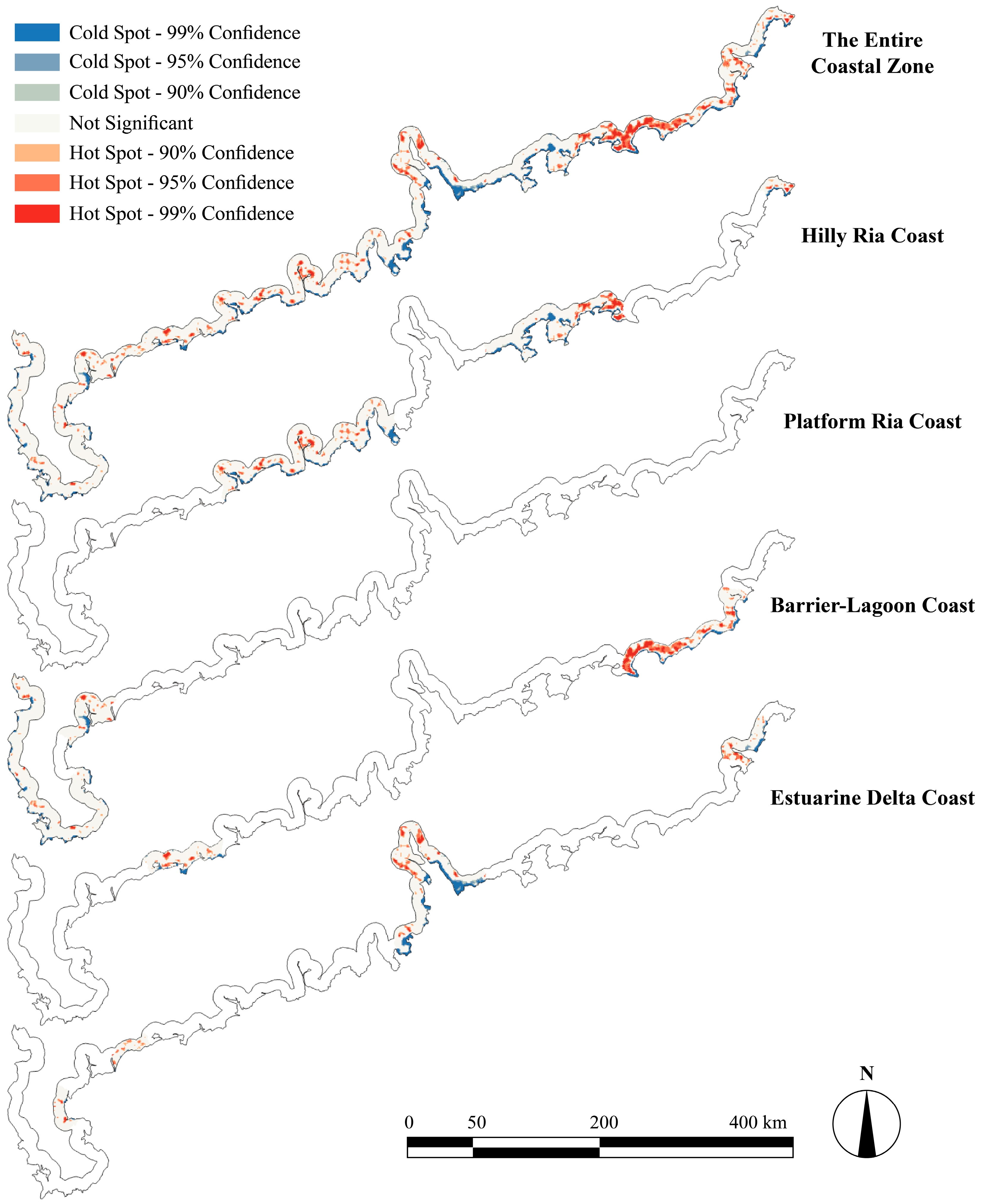
Further Gi* analysis reveals distinct local clustering patterns across coastal types (Figure 8). Cold spots show a consistent spatial pattern among all four coastal types, forming belt-like distributions along the coastline. These areas largely coincide with reclaimed tidal flats and aquaculture zones. In contrast, hot spots exhibit clear differences among geomorphic types:
- Hilly Ria Coast: Hotspots were scattered and concentrated near small-river estuaries (e.g., the Zhigong and Moyang rivers in Yangjiang; the Nafu River estuary in Jiangmen). Along eastern Guangdong, where mountains limit land available for development, hotspots clustered more densely near estuarine areas (e.g., Shanwei).
- Platform Ria Coast: Hotspots were few and spatially dispersed, located mainly near ports and reservoirs.
- Barrier–Lagoon Coast: Hotspots were strong and tightly clustered around lagoons, with extent and intensity increasing with lagoon area. Jieshi Bay (Lufeng) showed the most concentrated hotspots, consistent with the fragility of barrier–lagoon systems [49,50].
- Estuarine Delta Coast: Hotspots aligned with river networks and urban areas, following major rivers (e.g., the Pearl and Han) and intensifying around built-up zones.
Figure 8.
Hotspots and coldspots of coastal landscape ecological risk (shows only the specified coastal type; blank areas represent other coastal zones).
4.2.3. Temporal Evolution of Landscape Ecological Risk
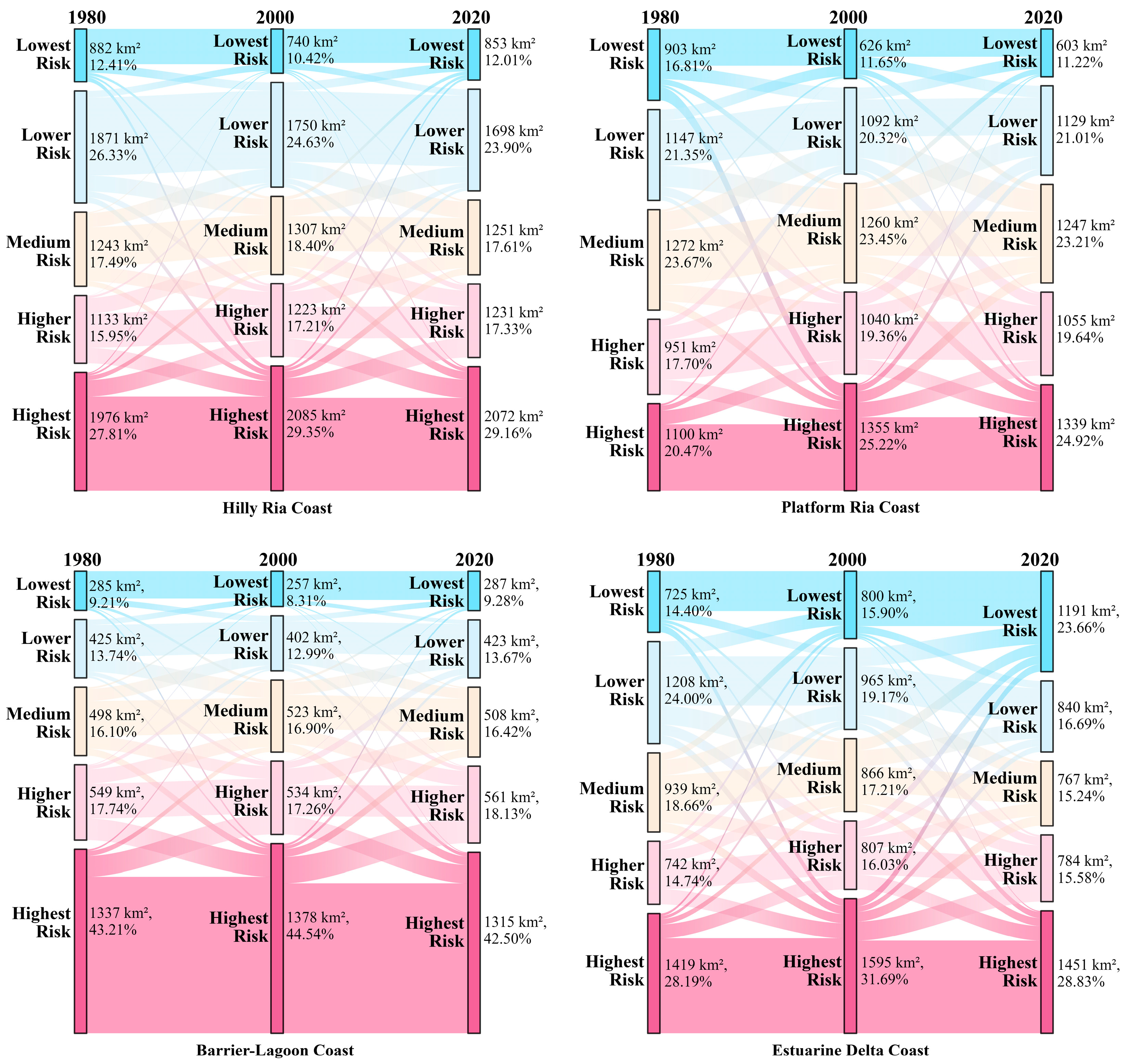
We quantified risk change using LERI differences (Figure 9) and summarized class transitions using Sankey diagrams based on transition matrices (Figure 10).
- Hilly Ria Coast: Risk increases were highly concentrated, forming an inward belt within coastal bays that largely overlapped with aquaculture zones. Risk decreases appeared as small, localized patches around urban areas. The highest risk class remained the largest and most stable (≈29%), while other classes shifted only modestly.
- Platform Ria Coast: Changes were strongly polarized. Risk increases formed a continuous coastal belt, while risk decreases were rare and scattered. The highest risk share rose from 20.47% to 24.92%, and the lowest risk share fell from 16.81% to 11.22%, indicating net risk intensification along the developed shoreline.
- Barrier–Lagoon Coast: Risk remained persistently high, with the highest risk class consistently exceeding 40%. Risk increases occurred mainly as small clusters near ports, whereas risk decreases concentrated around lagoons and river corridors.
- Estuarine Delta Coast: Despite being the most intensively developed region, it does not show the highest proportion of high-risk areas (≈29%), which contrasts with the common expectation that higher development intensity leads to higher ecological risk. Landscape ecological risk results from the combined effects of vulnerability and external pressure. Although the delta region has a high proportion of construction land and strong human disturbance, its land-use structure is relatively stable, and engineering and ecological management measures may have mitigated risk, resulting in a more optimized risk structure. This is supported by the increase in lowest-risk areas over 40 years (from 14.4% to 23.66%), indicating that risk has not continuously deteriorated. Sensitivity analysis (Table S13 in Supplementary Materials) shows that increasing the vulnerability of construction land raises LERI values, with a stronger response than in other coastal types. However, changes are mainly in magnitude, while spatial patterns remain highly consistent (Pearson’s r = 0.97–0.99). Overall, the risk pattern reflects the combined effects of intensive human activity and partial regulation, rather than model underestimation.
Figure 9.
Trend map of coastal landscape ecological risk change (shows only the specified coastal type; blank areas represent other coastal zones).
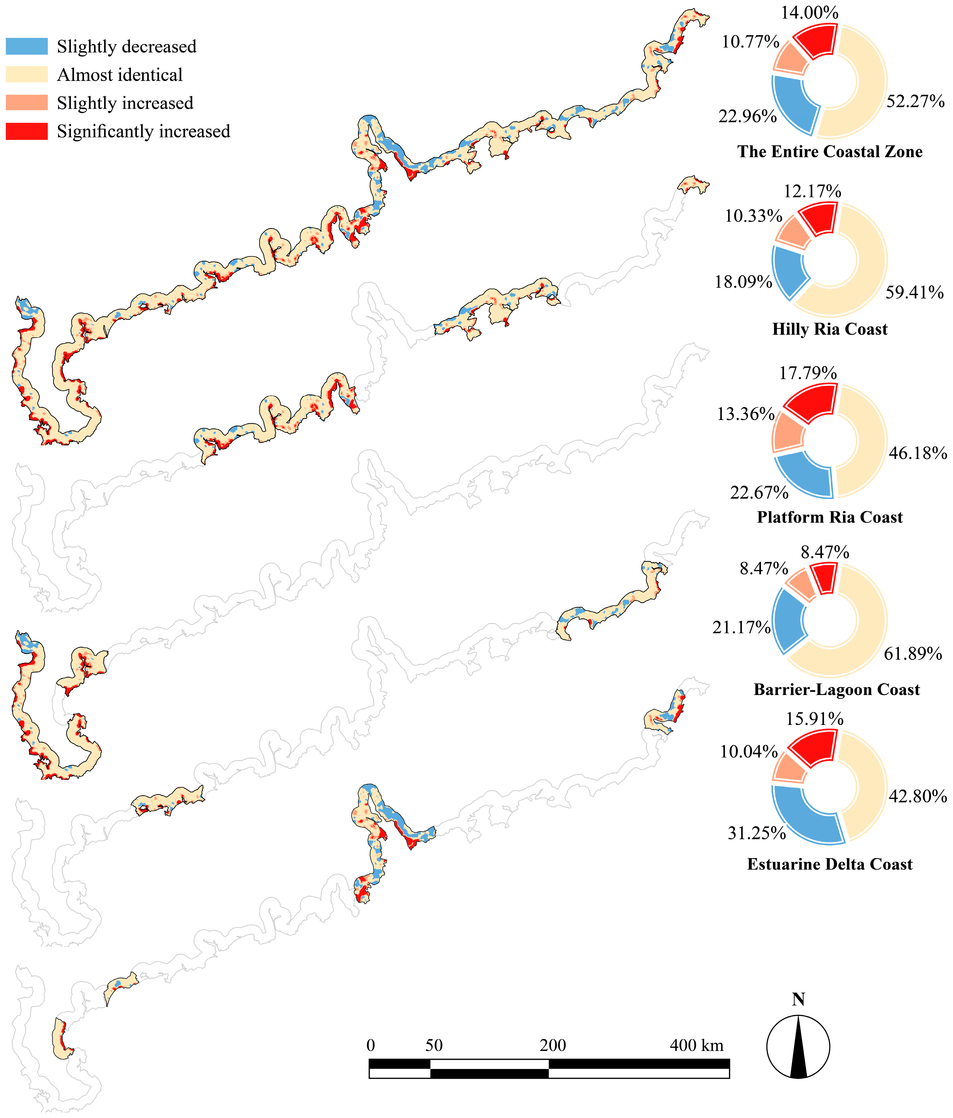
Figure 10.
Sankey diagrams (in km2) of the landscape ecological risk transition matrices for the four coastal types, 1980–2020.
4.3. Identification of Key Drivers of Coastal Landscape Ecological Risk
4.3.1. Factor Screening Based on Spatial Explanatory Power (OPGD)
Spatial heterogeneity in LERI was examined with the OPGD, combining factor detection (q-statistics) and interaction detection (Figure 11, Figure 12 and Figure 13, full results in Figures S12–S23 in Supplementary Materials). For each coastal type, the six highest-ranked factors are reported below.
- Hilly Ria Coast: The leading factors were NDVI (q = 0.504), slope (q = 0.426), DEM (q = 0.402), GDP (q = 0.349), distance to seaside (q = 0.339), and population density (q = 0.277). Interactions involving slope yielded the highest q-values; the strongest pair was slope ∩ GDP (q = 0.549). Nonlinear enhancement accounted for the majority of interaction types.
- Platform Ria Coast: The leading factors were DEM (q = 0.401), slope (q = 0.397), NDVI (q = 0.394), GDP (q = 0.209), population density (q = 0.182), and road network density (q = 0.127). Pairwise interaction strengths were weaker overall, with the lowest proportion of nonlinear-enhancement pairs among the four types (49.52%). The strongest pair was DEM ∩ GDP (q = 0.451).
- Barrier–Lagoon Coast: The leading factors were DEM (q = 0.590), NDVI (q = 0.503), GDP (q = 0.386), distance to seaside (q = 0.340), population density (q = 0.300), and slope (q = 0.263). This type showed the most active interactions, centered on DEM. DEM ∩ GDP was the strongest pair across all four types (q = 0.659).
- Estuarine Delta Coast: The leading factors were NDVI (q = 0.449), GDP (q = 0.309), DEM (q = 0.255), population density (q = 0.247), distance to seaside (q = 0.212), and slope (q = 0.149). Interactions were frequent but individually weaker than in other types; the strongest pair was GDP ∩ SLO (q = 0.447).
Figure 11.
Results of the OPGD factor detection, showing the independent explanatory power (q-statistic) of each factor for the spatial heterogeneity of landscape ecological risk.(DEM: Digital elevation model; SLO: Slope; SR: Surface Roughness; NDVI: Normalized Difference Vegetation Index; POP: Population Density; GDP: Gross Domestic Product; PCL: Proportion of Construction Land; RND: Road Network Density; HD: Distance to Harbor; SD: Distance to Seaside; RD: Distance to River; GD: Distance to Municipal/County Government; MFD: Distance to Tidal Flat/Mangrove; NRD: Distance to Nature Reserve; SSD: Distance to Strictly Protected Shoreline Section).
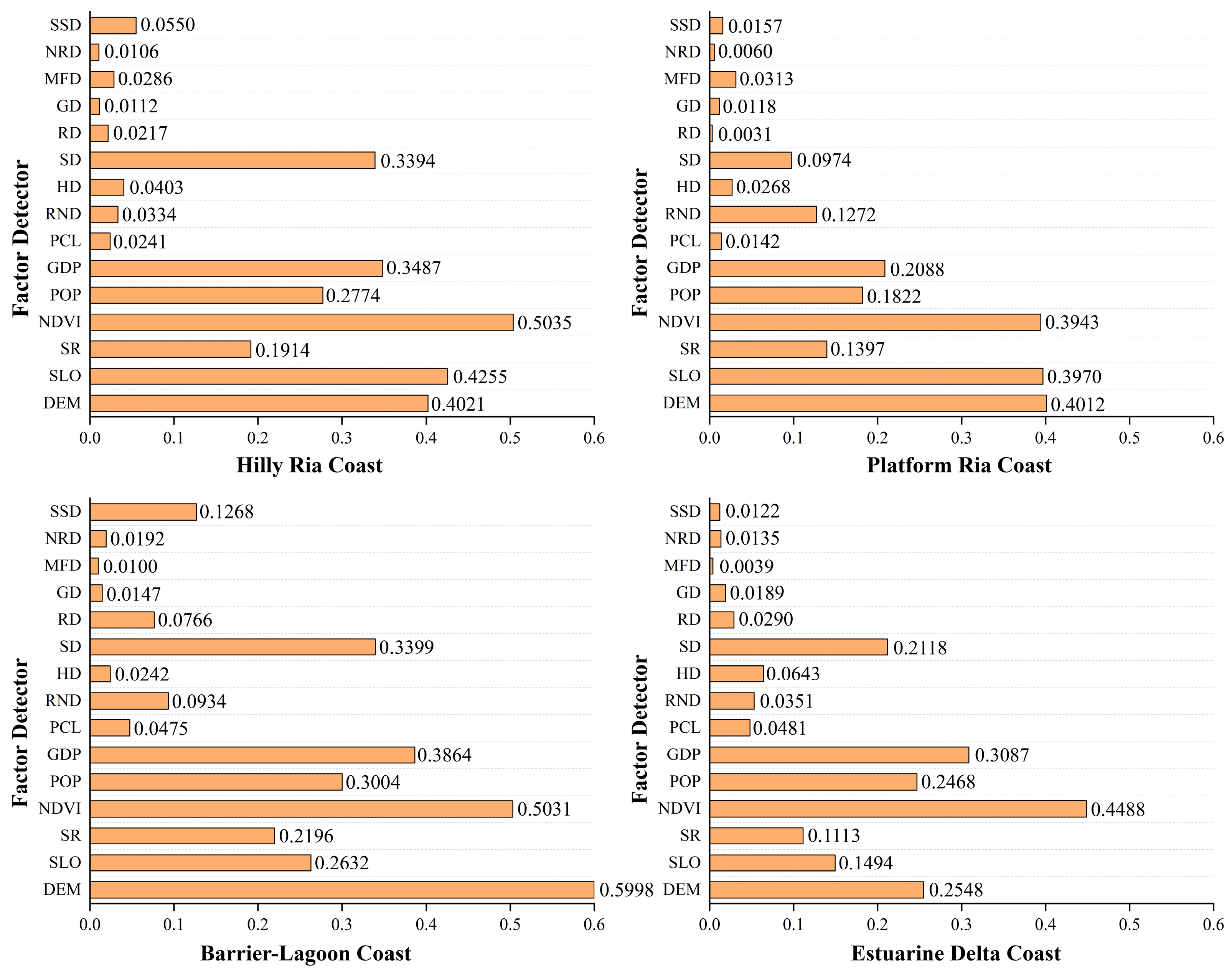
Figure 12.
Results of the OPGD ecological detection, revealing the types of interaction between factor pairs. (Abbreviation meanings are the same as in Figure 11).
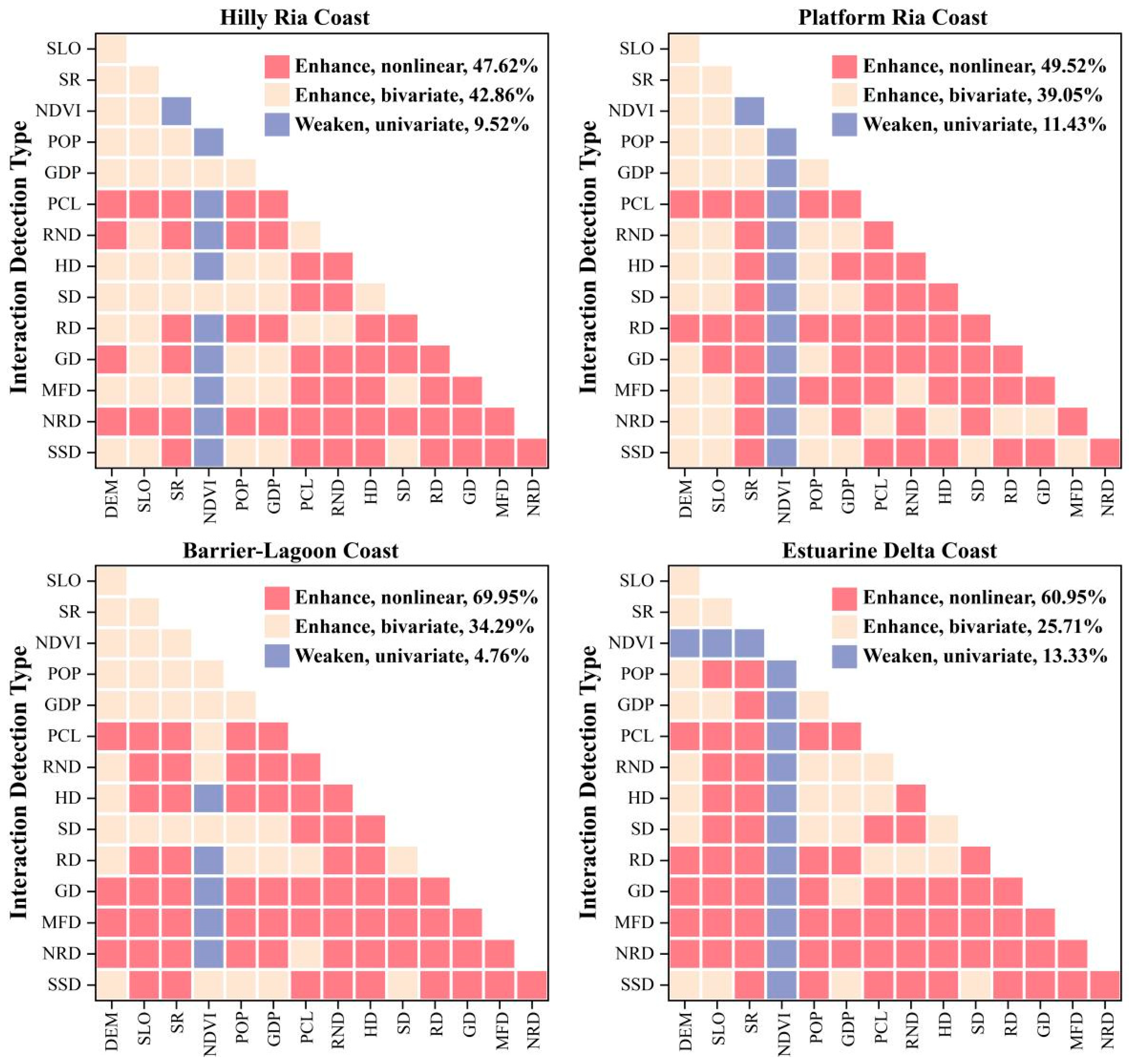
Figure 13.
Results of the OPGD interaction detection, revealing the strength of interaction between factor pairs. (No value shown due to nonsignificant interaction.Abbreviation meanings are the same as in Figure 11).
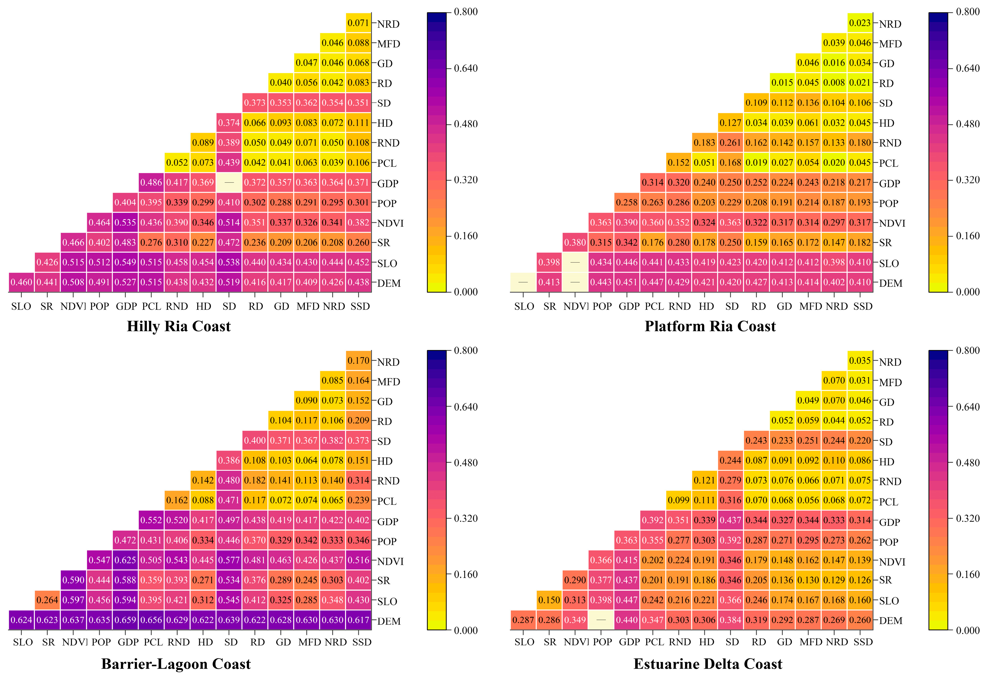
Across all four types, the top six factors accounted for the bulk of explained spatial differentiation, and nonlinear enhancement was the dominant interaction mode. However, the identity of the leading factor and the structure of interactions differed by geomorphic type: topographic variables (slope, DEM) ranked highest on Hilly Ria Coasts and Platform Ria Coasts, DEM dominated on Barrier–Lagoon Coasts, and NDVI and GDP led on Estuarine Delta Coasts.
4.3.2. Factor Validation Based on Predictive Contribution (XGBoost–SHAP)
XGBoost–SHAP was applied to assess each factor’s contribution to predicted LERI from a predictive perspective (Figure 14, key hyperparameters in Table S14 in Supplementary Materials; spatial cross-validation results in Table S15 in Supplementary Materials). The top six contributors for each type are reported below.
Figure 14.
SHAP contribution of driving factors to landscape ecological risk in the four coastal types. The bar length represents the mean absolute SHAP value of each factor, and the scatter points show the distribution of SHAP values for all samples. (Abbreviation meanings are the same as in Figure 11).
- Hilly Ria Coast: Slope (19.3%), distance to seaside (15.6%), GDP (12.4%), proportion of construction land (8.7%), DEM (8.1%), and road network density (6.4%). Four of these (slope, distance to seaside, GDP, DEM) overlapped with the OPGD top six. NDVI, ranked first by OPGD, fell outside the SHAP top six.
- Platform Ria Coast: Distance to seaside (14.7%), slope (14.3%), DEM (14.1%), GDP (7.3%), distance to tidal flat/mangrove (6.6%), and road network density (6.5%). DEM, slope, GDP, and road network density were shared with OPGD. NDVI and population density (important in OPGD) were replaced by distance to seaside and distance to tidal flat/mangrove.
- Barrier–Lagoon Coast: DEM (26.1%), distance to seaside (13.0%), proportion of construction land (10.4%), distance to nature reserve (8.3%), GDP (7.8%), and road network density (6.2%). DEM ranked first by a wide margin in both approaches. Compared with OPGD, SHAP gave higher ranks to proportion of construction land, road network density, and distance to nature reserve.
- Estuarine Delta Coast: GDP (18.0%), distance to seaside (14.2%), population density (12.6%), road network density (12.2%), proportion of construction land (9.1%), and slope (8.1%). This type showed the largest divergence from OPGD: NDVI and DEM, both highly ranked by OPGD, fell outside the SHAP top six. The SHAP ranking was dominated by socioeconomic and accessibility indicators.
4.3.3. Core Drivers Across Coastal Geomorphic Types
Combining OPGD rankings and interaction strengths with SHAP importance, we identified a core driver set for each type (Tables S16–S19 in Supplementary Materials):
- Hilly Ria Coast: NDVI, slope, DEM, distance to seaside.
- Platform Ria Coast: slope, DEM, NDVI, GDP.
- Barrier–Lagoon Coast: DEM, NDVI, GDP, distance to seaside.
- Estuarine Delta Coast: NDVI, GDP, population density, slope.
At least one topographic factor (slope or DEM) appeared in every set, but socioeconomic factors (GDP, population density) ranked higher on more heavily developed coasts—particularly the Estuarine Delta Coast—than on terrain-constrained coasts such as the Hilly Ria Coast. The mechanistic interpretation of these core drivers is addressed in the Discussion.
4.4. Nonlinear Responses and Statistical Thresholds of Key Driving Factors
It should be clarified that the “thresholds” identified using the RCS model represent points where the statistical relationship between driving factors and LERI changes significantly. The analysis is based on the averaged values of driving factors for 1980, 2000, and 2020, and thus reflects cross-sectional response patterns across different development stages and spatial conditions, rather than dynamic temporal tipping points. These thresholds indicate ranges where the sensitivity of LERI to changes in driving factors increases or decreases markedly. They can therefore serve as quantitative references for identifying risk-sensitive zones and supporting differentiated management strategies. However, these thresholds reflect statistical patterns derived from historical data and should not be interpreted as universal ecological thresholds indicating abrupt system shifts. Their application in practice requires validation under specific local conditions.
4.4.1. Hilly Ria Coast
NDVI showed an inverted U-shaped relationship with LERI, peaking at NDVI ≈ 0.624. Above this value, higher vegetation cover was associated with lower risk, consistent with a stronger ecological buffering role at denser canopy cover.
Slope exhibited a unimodal response, peaking at ~4.83° (LERI = 0.176). Below this value, steeper gradients were associated with greater erosion exposure and more intensive land-use pressure; above it, topographic constraints appear to limit development, and risk declined.
Elevation followed a similar inverted U-shape, with a turning point at ~229 m. Risk concentration at mid-elevations is consistent with greater overlap of human activity and terrain accessibility in this band.
Distance to seaside displayed a unimodal curve, peaking at ~3.2 km (LERI = 0.179) and declining at greater distances.
Across the four drivers (Figure 15), the highest LERI values occurred where NDVI was below 0.624, slope near 4.83°, elevation near 229 m, and distance to seaside near 3.2 km.
Figure 15.
Nonlinear responses and threshold identification of key driving factors in the Hilly Ria Coast. The upper panels show scatter plots and RCS fitted curves for NDVI, slope, elevation (DEM), and distance to seaside. The lower panels present the fitted RCS curves with corresponding confidence intervals. The vertical line indicates the statistically identified threshold.
4.4.2. Platform Ria Coast
Slope showed a unimodal relationship with LERI (Figure 16), peaking at ~2.8° and declining at steeper gradients. Below this value, small increases in slope corresponded to relatively large increases in risk; above it, the rate of change diminished.
Figure 16.
Nonlinear responses and threshold identification of key driving factors in the Platform Ria Coast. The upper panels show scatter plots and RCS fitted curves for slope, elevation (DEM), NDVI, and GDP. The lower panels present the fitted RCS curves with corresponding confidence intervals. The vertical line indicates the statistically identified threshold.
Elevation exhibited strong sensitivity at low altitudes. LERI peaked at ~14 m above sea level; within this low-elevation band, even modest topographic differences were associated with substantial variation in risk.
NDVI displayed an inverted U-shaped curve, with the highest risk at NDVI ≈ 0.6. Below this value, increasing vegetation cover tracked with rising risk; above it, denser cover was associated with progressively lower risk.
GDP exhibited an inverted U-shaped relationship with LERI, reaching a maximum value of 0.167 at approximately 554.350 × 10⁶ CNY/km2. Beyond this point, the rate of increase diminished and risk began to decline slightly, suggesting a potential transition toward more regulated or efficient development stages.
The highest LERI in this type tended to occur under low elevation (<14 m), gentle slopes (~2.8°), moderate vegetation cover (NDVI ≈ 0.6), and moderate economic intensity (GDP ≈ 554 × 106 CNY/km2).
4.4.3. Barrier–Lagoon Coast
Elevation was the strongest single control (Figure 17). LERI rose to a maximum at ~14.54 m (LERI = 0.178), then declined and stabilized at ~0.151 above 105.67 m. The steep response at low elevations is consistent with greater exposure to storm-surge flooding and more intensive land use in low-lying areas. Above 105.67 m, risk was comparatively stable.
Figure 17.
Nonlinear responses and threshold identification of key driving factors in the Barrier–Lagoon Coast. The upper panels show scatter plots and RCS fitted curves for elevation (DEM), NDVI, GDP, and distance to seaside. The lower panels present the fitted RCS curves with corresponding confidence intervals. The vertical line indicates the statistically identified threshold.
NDVI showed a non-monotonic response. LERI was lowest at NDVI ≈ 0.102 (LERI = 0.124) and highest at NDVI ≈ 0.539 (LERI = 0.172). The low risk at very low NDVI corresponds to bare or built-up surfaces, while the peak at moderate NDVI may correspond to fragmented semi-natural cover under active disturbance. A consistent risk-reducing association appeared only above NDVI ≈ 0.652.
GDP showed an N-shaped response. LERI increased with GDP density and peaked at ~293.31 × 10⁶ CNY/km2 (LERI = 0.175). It then declined to a minimum at ~1034.13 × 106 CNY/km2 (LERI = 0.157), followed by a gradual rebound. This trajectory suggests stage-dependent effects of economic development. During early industrialization, risk increases rapidly due to land conversion and resource-intensive activities. As development proceeds, structural upgrading (e.g., a shift toward services/tourism) and improved environmental management may temporarily reduce risk. Beyond a certain intensity threshold, cumulative anthropogenic pressure can be associated with risk upward again. A nonlinear relationship is observed between GDP and landscape ecological risk. This pattern is consistent with the Environmental Kuznets Curve (EKC) theory, which suggests that economic development and environmental pressure may exhibit a nonlinear relationship [51].
Distance to seaside followed a unimodal curve, peaking at ~3.57 km (LERI = 0.181) and declining at greater distances.
The highest LERI in this type was associated with low elevation (<14.54 m), moderate NDVI (~0.539), intermediate GDP density (~293 × 106 CNY/km2), and distance to seaside near 3.57 km.
4.4.4. Estuarine Delta Coast
NDVI showed a U-shaped relationship with LERI (Figure 18). Risk was relatively low at very low NDVI (~0; LERI = 0.127), corresponding to built-up or bare surfaces, and peaked at NDVI ≈ 0.447 (LERI = 0.163), a range typical of intensively managed semi-natural cover. At higher NDVI, risk declined, suggesting that only well-established vegetation provides a consistent buffering effect in this heavily developed setting.
Figure 18.
Nonlinear responses and threshold identification of key driving factors in the Estuarine Delta Coast. The upper panels show scatter plots and RCS fitted curves for NDVI, GDP, population density, and slope. The lower panels present the fitted RCS curves with corresponding confidence intervals. The vertical line indicates the statistically identified threshold.
GDP and population density both exhibited inverted U-shaped curves. LERI peaked at GDP ≈ 1645 × 106 CNY/km2 (LERI = 0.166) and at population density ≈ 1620 persons km−2 (LERI = 0.166). The near-coincident peaks indicate a socioeconomic intensity range in which the combined pressure of land conversion, pollution loading, and landscape fragmentation is greatest. Beyond these values, risk declined, possibly because the most intensively developed areas have already undergone land-cover stabilization.
Slope, despite the flat terrain, showed a unimodal response peaking at ~2.38° (LERI = 0.162). Even small topographic differences appear to concentrate settlement and infrastructure siting in deltaic settings, which may account for the risk peak at such a gentle gradient.
The highest LERI in this type occurred under moderate NDVI (~0.447), high socioeconomic intensity (GDP ~1645 × 106 CNY/km2; population density ~1620 persons km−2), and gentle slopes (~2.38°).
5. Discussion
5.1. Shared Drivers of Coastal Landscape Ecological Risk and Management Implications
Understanding the common drivers and spatial organization of ecological risk is essential for designing flexible, context-specific adaptive management strategies.
- (1)
- Convergence of key drivers across geomorphic types
Although dominant mechanisms vary among the four geomorphic types, the core drivers converge along three consistent axes: the natural matrix (NDVI, DEM, slope), anthropogenic pressure (population density, GDP), and the land–sea position gradient (distance to seaside). This tripartite structure aligns with the Pressure–State–Response framework [52] and coastal human–environment system theory [53,54], indicating that risk formation follows a shared architecture rather than arising from purely site-specific factors. What differs across types is how geomorphic setting modulates the relative importance and interactions of these drivers—producing the distinct mechanisms detailed in Section 5.3.
- (2)
- Why “Conservation and policy constraints” variables show limited effects
The results show that factors representing ecological protection (e.g., distance to tidal flats/mangroves, marine reserves, and strictly protected shoreline sections) have relatively low statistical contributions in the model. This may be partly attributed to the construction of the landscape ecological risk index (LERI), in which protection-related variables are not directly incorporated. Therefore, their lower importance in the model does not necessarily imply limited ecological effects, but may reflect their underrepresentation in the current indicator system. In addition, landscape ecological risk exhibits spatial spillover effects. The influence of protected areas may operate through neighboring regions and is not fully captured by simple distance-based variables. Thus, the results should be interpreted as indicating a statistical association, rather than a lack of ecological management significance.
These findings also suggest that a protection strategy primarily based on point- and line-based protected areas may be insufficient to represent regional risk patterns. Previous studies have shown that ecological processes are strongly influenced by spatial connectivity and scale dependence. Single protected areas may therefore be limited in addressing cross-regional risk transmission. From a management perspective, it is necessary to strengthen ecological network construction and spatial connectivity, building on existing protection systems. This aligns with the principles of landscape ecological security patterns [55] and integrated coastal zone management [56], as well as the goal of establishing an ecological security network in the Guangdong Coastal Zone Plan. The present study provides a basis for identifying key nodes (high-risk areas) and optimizing corridor pathways, thereby supporting the translation of strategic planning into spatially explicit management actions.
5.2. Differences Between OPGD and XGBoost–SHAP: A Dual-Layer Response Structure of Coastal Landscape Ecological Risk
This study integrates OPGD and XGBoost–SHAP for driving factor analysis. Their value lies not only in cross-validation, but also in the differences between their results, which reveal distinct driving mechanisms. These differences mainly arise from their theoretical foundations and analytical perspectives. OPGD is based on spatial stratified heterogeneity and identifies factors that explain spatial patterns of risk. In contrast, XGBoost–SHAP focuses on predictive contributions and explains variations in local risk values. Therefore, differences in factor importance primarily reflect methodological distinctions rather than purely ecological mechanisms.
From an ecological perspective, this difference can be interpreted as a pattern–process distinction. OPGD explains how the spatial pattern of risk is formed, with key factors representing structural geographic conditions. XGBoost–SHAP explains how risk levels vary at specific locations, with high-contribution factors reflecting variables that directly influence local risk variation. Consistency between the two methods (e.g., DEM in the Barrier–Lagoon Coast) indicates factors that are important at both levels, whereas discrepancies suggest a separation between pattern- and process-driven controls.
In the Estuarine Delta Coast, for example, OPGD identifies NDVI as the dominant factor explaining spatial differentiation, highlighting the role of ecological land in shaping the overall safety pattern. In contrast, XGBoost–SHAP identifies GDP and population density as key predictors of risk levels, emphasizing the strong influence of human activities. This difference reflects a dual-layer structure: a relatively stable risk pattern defined by ecological space, and a dynamic risk level driven by socioeconomic activity. Together, these layers explain both where risk occurs and why it is high.
Therefore, the value of this framework lies not in producing a single ranking of factors, but in revealing differences in factor importance across analytical perspectives. This distinction helps separate structural and process-based drivers and improves the understanding of coastal ecological risk complexity. It also provides a basis for more targeted management strategies.
5.3. Geomorphic-Specific Adaptive Management Strategies
The four dominant patterns and associated response thresholds identified in this study provide a basis for moving beyond uniform management toward geomorphology-adaptive governance. Although coastal management in Guangdong has incorporated concepts such as zoning and land–sea integration, the criteria for classification and the degree of differentiation remain insufficiently quantified. This study offers quantitative evidence to support both classification and the definition of differentiated management thresholds.
It should be noted that the LERI used here is a composite indicator based on landscape pattern and vulnerability weighting, reflecting statistical spatial patterns of risk. Mechanistic interpretations are inferred from observed patterns, and the identified thresholds represent points of significant change in statistical relationships. These thresholds should therefore be interpreted as indicative ranges of risk sensitivity rather than fixed ecological limits. In practice, they provide a reference for identifying priority areas and guiding differentiated management. Under this framework, the results can be translated into geomorphology-specific management implications.
In the Hilly Ria Coast, risk is constrained by fragile valley ecosystems and steep terrain. Management may prioritize the coupling of ecological restoration and topographic constraints. Sensitive ranges (e.g., NDVI > 0.624; slope > 25°) can be treated as indicative conditions for enhanced protection, while low-slope zones (<4.83°) may be comparatively more suitable for carefully managed activities, subject to site-specific assessment.
In the Platform Ria Coast, risk is associated with concentrated development in limited favorable terrain. Management may combine spatial zoning with development intensity guidance. Low-elevation areas (<14 m) and gentle slopes (~2.8°) may warrant closer monitoring or precautionary management, while construction land proportion (PCL ≤ 15.5%) can be used as an indicative reference in planning decisions rather than a strict cap.
In the Barrier–Lagoon Coast, risk is strongly constrained by elevation, with low-lying areas (DEM < 14.54 m) exhibiting high inherent risk. Given existing development, strict exclusion is often impractical. Management may therefore emphasize adaptive risk reduction, focusing on mitigation in built-up areas while conserving remaining natural shoreline and ecological space where feasible.
In the Estuarine Delta Coast, intensive human–environment interactions dominate. A dual reference framework of development intensity and ecological buffering may be useful. In higher-intensity zones (e.g., GDP density > 1.644 × 10⁹ CNY/km2; population density > 1619 persons/km2), these values may serve as early-warning references for intensified risk management, while maintaining ecological buffer areas (NDVI > 0.447) may support system resilience.
Overall, this study supports a shift from uniform indicator-based management toward spatially responsive management informed by geomorphological patterns and quantitative statistical thresholds. It provides a basis for identifying where management attention may be prioritized, which factors may be most influential, and what value ranges may serve as context-dependent references, thereby supporting more adaptive and evidence-informed coastal governance.
5.4. Contributions and Limitations
This study develops a hierarchical framework of “spatiotemporal patterns–driving processes–response thresholds”. From a geomorphological perspective, it integrates an OPGD–XGBoost–SHAP–RCS method chain to reveal differentiated patterns, nonlinear mechanisms, and potential thresholds of coastal landscape ecological risk, providing a pathway from assessment to targeted management.
- (1)
- Main advances
A geomorphological perspective is introduced as a “background filter” that reshapes driving effects. Four dominant pattern types are identified, shifting the focus from individual factors to mechanism-based classification. The method chain enables hierarchical decomposition of drivers: OPGD identifies pattern-related factors, SHAP captures process-related contributions, and RCS quantifies nonlinear thresholds. The resulting threshold system (e.g., NDVI thresholds of 0.624 for the Hilly Ria Coast and 0.447 for the Estuarine Delta Coast) provides spatial guidance on where which factors, and to what extent management should be applied.
- (2)
- Transferability of the framework
Although thresholds are context-dependent, the framework is transferable. By integrating spatial analysis, machine learning, and nonlinear modeling, it captures nonlinear relationships between development and ecological risk. It can be adapted to other regions through recalibration of variables and thresholds.
- (3)
- Limitations and outlook
Several limitations remain. First, vulnerability assignment, although relatively robust, still involves empirical judgment. Future work could incorporate more objective indicators (e.g., ecosystem services, resilience, or adaptive capacity) to develop process-based assessments. Second, some variables (e.g., construction land proportion) are partly related to the risk index, introducing potential conceptual overlap. However, this effect is limited and reflects the linkage between landscape structure and risk. The analysis therefore focuses on associations rather than strict causality.
6. Conclusions
This study integrates landscape metrics, GIS-based gridding, the LERI model, OPGD, XGBoost–SHAP, and restricted cubic spline (RCS) modeling to develop a “pattern–process–threshold” framework. This framework is used to analyze the spatiotemporal patterns, driving mechanisms, and response thresholds of landscape ecological risk across multiple coastal types in Guangdong, China. The main conclusions are as follows:
- (1)
- The spatiotemporal patterns of landscape ecological risk show strong geomorphological dependence. Significant differences are observed among the four coastal types (Hilly Ria, Platform Ria, Barrier–Lagoon, and Estuarine Delta) in terms of spatial clustering, temporal evolution, and dominant drivers. This confirms that geomorphology acts as a fundamental control on risk patterns, and treating coastal zones as homogeneous units may obscure inherent heterogeneity.
- (2)
- The driving mechanisms exhibit a “shared framework with type-specific combinations”. Although natural conditions, human activities, and coastal location form common driving dimensions, their relative importance, interactions, and nonlinear effects vary across geomorphic types, forming four distinct mechanism patterns. This highlights the complexity of coastal human–environment systems and the need for context-specific interpretation.
- (3)
- Statistically derived response thresholds linked to geomorphological mechanisms are identified, providing quantitative references for differentiated management. Nonlinear modeling reveals key threshold values, such as NDVI ≈ 0.624 in the Hilly Ria Coast, slope ≈ 2.8° in the Platform Ria Coast, elevation ≈ 14.5 m in the Barrier–Lagoon Coast, and GDP ≈ 1644.65 × 106 CNY/km2 in the Estuarine Delta Coast. These thresholds represent statistical inflection points in risk sensitivity rather than fixed ecological limits, and serve as spatial references for identifying priority areas and key control factors.
- (4)
- The contributions of this study are threefold. Theoretically, it demonstrates the importance of geomorphological stratification in understanding coastal risk patterns. Methodologically, the integrated OPGD–XGBoost–SHAP–RCS framework enables coordinated analysis of spatial heterogeneity, nonlinear relationships, and thresholds. Practically, it provides a quantitative basis for differentiated and spatially explicit coastal management.
Supplementary Materials
The following supporting information can be downloaded at: https://www.mdpi.com/article/10.3390/land15050729/s1, Table S1: Representative Landscape Indices and Their Significance; Table S2: Rationale for the Selection of Different Analysis Extents; Table S3: Vulnerability assignment and rationale for coastal landscape types; Table S4: Variation of PD semivariogram with spatial extent in the Hilly Ria Coast; Table S5: Variation of SHDI semivariogram with spatial extent in the Hilly Ria Coast; Table S6: Variation of PD semivariogram with spatial extent in the Platform Ria Coast; Table S7: Variation of SHDI semivariogram with spatial extent in the Platform Ria Coast; Table S8: Variation of PD semivariogram with spatial extent in the Barrier–Lagoon Coast; Table S9: Variation of SHDI semivariogram with spatial extent in the Barrier–Lagoon Coast; Table S10: Variation of PD semivariogram with spatial extent in the Estuarine Delta Coast; Table S11: Variation of SHDI semivariogram with spatial extent in the Estuarine Delta Coast; Table S12: Sensitivity analysis of unified versus optimal scales across four coastal types; Table S13: Sensitivity analysis of construction land vulnerability scenarios on LERI; Table S14: Key hyperparameters of the XGBoost model; Table S15: Spatial cross-validation (CV) results of the XGBoost model; Table S16: Rationale for Selecting Key Factors in the Hilly Ria Coast; Table S17: Rationale for Selecting Key Factors in the Platform Ria Coast; Table S18: Rationale for Selecting Key Factors in the Barrier-Lagoon Coast; Table S19: Rationale for Selecting Key Factors in the Estuarine Delta Coast; Figure S1: Response curves of landscape metrics to increasing grid size in the Hilly Ria Coast; Figure S2: Information loss of landscape patterns at different grain sizes in the Hilly Ria Coast; Figure S3: Response curves of landscape metrics to increasing grid size in the Platform Ria Coast; Figure S4: Information loss of landscape patterns at different grain sizes in the Platform Ria Coast; Figure S5: Response curves of landscape metrics to increasing grid size in the Barrier–Lagoon Coast; Figure S6: Information loss of landscape patterns at different grain sizes in the Barrier–Lagoon Coast; Figure S7: Response curves of landscape metrics to increasing grid size in the Estuarine Delta Coast; Figure S8: Information loss of landscape patterns at different grain sizes in the Estuarine Delta Coast; Figure S9: Moran’s I results under different construction land vulnerability scenarios (values 2–4); Figure S10: Moran’s I Scatter Plot; Figure S11: Moran’s I Summary. Figure S12: Optimal discretization schemes of explanatory variables in the OPGD model for the Hilly Ria Coast; Figure S13: Classification results of explanatory variables in the OPGD model for the Hilly Ria Coast; Figure S14: Factor detection results of individual variables on LERI using the OPGD model in the Hilly Ria Coast; Figure S15: Optimal discretization schemes of explanatory variables in the OPGD model for the Platform Ria Coast; Figure S16: Classification results of explanatory variables in the OPGD model for the Platform Ria Coast; Figure S17: Factor detection results of individual variables on LERI using the OPGD model in the Platform Ria Coast; Figure S18: Optimal discretization schemes of explanatory variables in the OPGD model for the Barrier–Lagoon Coast; Figure S19: Classification results of explanatory variables in the OPGD model for the Barrier–Lagoon Coast; Figure S20: Factor detection results of individual variables on LERI using the OPGD model in the Barrier–Lagoon Coast; Figure S21: Optimal discretization schemes of explanatory variables in the OPGD model for the Estuarine Delta Coast; Figure S22: Classification results of explanatory variables in the OPGD model for the Estuarine Delta Coast; Figure S23: Factor detection results of individual variables on LERI using the OPGD model in the Estuarine Delta Coast.
Author Contributions
Conceptualization, S.F.; methodology, S.F.; software, S.F.; validation, Y.S.; formal analysis, S.F.; investigation, S.F.; resources, Y.P.; data curation, S.F.; writing—original draft preparation, S.F.; writing—review and editing, Y.P. and Y.S.; visualization, S.F.; supervision, Y.S.; project administration, Y.P.; funding acquisition, Y.P. All authors have read and agreed to the published version of the manuscript.
Funding
This research was funded by the Independent Research Project of the State Key Laboratory of Subtropical Building and Urban Science (Grant No. 2023ZB09) and the Guangdong Basic and Applied Basic Research Foundation (Grant No. 2025A1515011540).
Data Availability Statement
The data presented in this study are available upon request from the corresponding author.
Conflicts of Interest
The authors declare no conflicts of interest.
References
- Neumann, B.; Ott, K.; Kenchington, R. Strong sustainability in coastal areas: A conceptual interpretation of SDG 14. Sustain. Sci. 2017, 12, 1019–1035. [Google Scholar] [CrossRef] [Scilit] [PubMed]
- Sterzel, T.; Lüdeke, M.K.B.; Walther, C.; Kok, M.T.; Sietz, D.; Lucas, P.L. Typology of coastal urban vulnerability under rapid urbanization. PLoS ONE 2020, 15, e0220936. [Google Scholar] [CrossRef] [Scilit] [PubMed]
- Alizad, K.; Hagen, S.C.; Morris, J.T.; Medeiros, S.C.; Bilskie, M.V.; Weishampel, J.F. Coastal wetland response to sea-level rise in a fluvial estuarine system. Earth’s Future 2016, 4, 483–497. [Google Scholar] [CrossRef] [Scilit]
- Biondo, M.; Buosi, C.; Trogu, D.; Mansfield, H.; Vacchi, M.; Ibba, A.; Porta, M.; Ruju, A.; De Muro, S. Natural vs. anthropic influence on the multidecadal shoreline changes of Mediterranean urban beaches: Lessons from the Gulf of Cagliari (Sardinia). Water 2020, 12, 3578. [Google Scholar] [CrossRef] [Scilit]
- Guo, H.; Cai, Y.; Li, B.; Wan, H.; Yang, Z. An improved approach for evaluating landscape ecological risks and exploring its coupling coordination with ecosystem services. J. Environ. Manag. 2023, 348, 119277. [Google Scholar] [CrossRef] [Scilit]
- Li, Y.; Sun, X.; Zhu, X.; Cao, H. An early warning method of landscape ecological security in rapid urbanizing coastal areas and its application in Xiamen, China. Ecol. Model. 2010, 221, 2251–2260. [Google Scholar] [CrossRef] [Scilit]
- Liu, L.; Wei, J.; Luo, P.; Zhang, Y.; Wang, Y.; Elbeltagi, A.; Zainol, M.R.R.M.A. A novel quantity assessment of landscape ecological risk using human-nature driving mechanism for sustainable society. Sci. Total Environ. 2024, 947, 173892. [Google Scholar] [CrossRef] [Scilit]
- Wang, G.; Ran, G.; Chen, Y.; Zhang, Z. Landscape ecological risk assessment for the Tarim River Basin on the basis of land-use change. Remote Sens. 2023, 15, 4173. [Google Scholar] [CrossRef] [Scilit]
- Ma, Z.; Gao, J.; Liang, T.; He, Z.; Feng, S.; Zhang, X.; Zhang, D. Comprehensive ecological risk changes and their relationship with ecosystem services of alpine grassland in Gannan prefecture from 2000–2020. Remote Sens. 2024, 16, 2242. [Google Scholar] [CrossRef] [Scilit]
- Karimian, H.; Zou, W.; Chen, Y.; Xia, J.; Wang, Z. Landscape ecological risk assessment and driving factor analysis in Dongjiang river watershed. Chemosphere 2022, 307, 135835. [Google Scholar] [CrossRef] [Scilit]
- Shamuxi, A.; Han, B.; Jin, X.; Wusimanjiang, P.; Abudukerimu, A.; Chen, Q.; Zhou, H.; Gong, M. Spatial pattern and driving mechanisms of dryland landscape ecological risk: Insights from an integrated geographic detector and machine learning model. Ecol. Indic. 2025, 172, 113305. [Google Scholar] [CrossRef] [Scilit]
- Gao, B.; Wu, Y.; Li, C.; Zheng, K.; Wu, Y.; Wang, M.; Fan, X.; Ou, S. Multi-Scenario Prediction of Landscape Ecological Risk in the Sichuan-Yunnan Ecological Barrier Based on Terrain Gradients. Land 2022, 11, 2079. [Google Scholar] [CrossRef] [Scilit]
- Lin, X.; Wang, Z. Landscape ecological risk assessment and its driving factors of multi-mountainous city. Ecol. Indic. 2023, 146, 109823. [Google Scholar] [CrossRef] [Scilit]
- Wang, X.; Sun, Y.; Liu, Q.; Zhang, L. Construction and Optimization of Ecological Network Based on Landscape Ecological Risk Assessment: A Case Study in Jinan. Land 2023, 12, 743. [Google Scholar] [CrossRef] [Scilit]
- Wang, J.; Wang, J.; Zhang, J. Optimization of landscape ecological risk assessment method and ecological management zoning considering resilience. J. Environ. Manag. 2025, 376, 124586. [Google Scholar] [CrossRef] [Scilit]
- Li, J.; Hu, D.; Wang, Y.; Chu, J.; Yin, H.; Ma, M. Study of identification and simulation of ecological zoning through integration of landscape ecological risk and ecosystem service value. Sustain. Cities Soc. 2024, 107, 105442. [Google Scholar] [CrossRef] [Scilit]
- Du, L.; Dong, C.; Kang, X.; Qian, X.; Gu, L. Spatiotemporal evolution of land cover changes and landscape ecological risk assessment in the Yellow River Basin, 2015–2020. J. Environ. Manag. 2023, 332, 117149. [Google Scholar] [CrossRef] [Scilit]
- Ai, J.; Yu, K.; Zeng, Z.; Yang, L.; Liu, Y.; Liu, J. Assessing the dynamic landscape ecological risk and its driving forces in an island city based on optimal spatial scales: Haitan Island, China. Ecol. Indic. 2022, 137, 108771. [Google Scholar] [CrossRef] [Scilit]
- Wang, X.; Zhu, T.; Jiang, C. Landscape ecological risk based on optimal scale and its tradeoff/synergy with human activities: A case study of the Nanjing metropolitan area, China. Ecol. Indic. 2025, 170, 113040. [Google Scholar] [CrossRef] [Scilit]
- Li, M.; Abuduwaili, J.; Liu, W.; Feng, S.; Saparov, G.; Ma, L. Application of geographical detector and geographically weighted regression for assessing landscape ecological risk in the Irtysh River Basin, Central Asia. Ecol. Indic. 2024, 158, 111540. [Google Scholar] [CrossRef] [Scilit]
- Li, S.; He, W.; Wang, L.; Zhang, Z.; Chen, X.; Lei, T.; Wang, S.; Wang, Z. Optimization of landscape pattern in China Luojiang Xiaoxi basin based on landscape ecological risk assessment. Ecol. Indic. 2023, 146, 109887. [Google Scholar] [CrossRef] [Scilit]
- Gong, J.; Cao, E.; Xie, Y.; Xu, C.; Li, H.; Yan, L. Integrating ecosystem services and landscape ecological risk into adaptive management: Insights from a western mountain-basin area, China. J. Environ. Manag. 2021, 281, 111817. [Google Scholar] [CrossRef] [Scilit]
- Qiao, B.; Yang, H.; Cao, X.; Zhou, B.; Wang, N. Driving mechanisms and threshold identification of landscape ecological risk: A nonlinear perspective from the Qilian Mountains, China. Ecol. Indic. 2025, 173, 113342. [Google Scholar] [CrossRef] [Scilit]
- Zhu, K.; He, J.; Zhang, L.; Song, D.; Wu, L.; Liu, Y.; Zhang, S. Impact of Future Development Scenario Selection on Landscape Ecological Risk in the Chengdu-Chongqing Economic Zone. Land 2022, 11, 964. [Google Scholar] [CrossRef] [Scilit]
- Xu, W.; Yao, W.; Wang, H.; Yang, J.; Yu, T.; Yu, H. Assessing Landscape Ecological Risk from Mining in the River Source Region of the Yellow River Basin. Land 2025, 14, 2152. [Google Scholar] [CrossRef] [Scilit]
- Ayre, K.K.; Landis, W.G. A Bayesian approach to landscape ecological risk assessment applied to the Upper Grande Ronde Watershed, Oregon. Hum. Ecol. Risk Assess. Int. J. 2012, 18, 946–970. [Google Scholar] [CrossRef] [Scilit]
- Hu, G.; Guo, Y.; Zhang, C.; Chen, Y.; Lang, Y.; Su, L.; Huang, H. Landscape ecological risk assessment of the northern coastal region of China based on the improved ESRISK framework: A case study of Cangzhou City. Ecol. Indic. 2025, 171, 113222. [Google Scholar] [CrossRef] [Scilit]
- Fang, J.; Xu, M. A novel ecological risk assessment approach applied to Jiangsu coastal zone, China. Ocean Coast. Manag. 2023, 244, 106815. [Google Scholar] [CrossRef] [Scilit]
- Zhai, J.; Pu, L.; Qie, L.; He, G.; Wang, X.; Zhang, R.; Yuan, Y.; Zhong, R.; Lu, Y.; Xie, J.; et al. Changes of land use and landscape pattern along sea–land gradient in developed coastal region: A case study of Jiangsu Province, China. Ecol. Indic. 2025, 176, 113635. [Google Scholar] [CrossRef] [Scilit]
- Xu, M.; Matsushima, H. Multi-dimensional landscape ecological risk assessment and its drivers in coastal areas. Sci. Total Environ. 2024, 908, 168183. [Google Scholar] [CrossRef] [Scilit]
- Li, N.; Wang, Z. Nonlinear influence mechanism and threshold effect of seaport scale on the high–quality development of coastal port cities. Geogr. Geo-Inf. Sci. 2026, 42, 97–104. [Google Scholar] [CrossRef]
- Yan, X.; Wei, C.; Sun, Y.; Hu, Y. Nonlinear Thresholds in Carbon–Water Functional Synergies under Coastal Reclamation in the Liaohe River Delta, China. Estuaries Coasts 2026, 49, 62. [Google Scholar] [CrossRef] [Scilit]
- Dar, S.A.; Dar, J.A. Trade-offs in ecosystem services of a Ramsar wetland due to conversion into aquaculture ponds in the coastal region of Indian peninsula. Ocean Coast. Manag. 2025, 269, 107861. [Google Scholar] [CrossRef] [Scilit]
- Li, D.; Cao, W.; Dou, Y.; Wu, S.; Liu, J.; Li, S. Non-linear effects of natural and anthropogenic drivers on ecosystem services: Integrating thresholds into conservation planning. J. Environ. Manag. 2022, 321, 116047. [Google Scholar] [CrossRef] [Scilit]
- Zhao, X.; Xu, Y.; Pu, J.; Tao, J.; Chen, Y.; Huang, P.; Shi, X.; Ran, Y.; Gu, Z. Achieving the supply-demand balance of ecosystem services through zoning regulation based on land use thresholds. Land Use Policy 2024, 139, 107056. [Google Scholar] [CrossRef] [Scilit]
- Zeng, Z.X.; Huang, W.F. Natural Geography of Guangdong (2001); Guangdong People’s Publishing House: Guangzhou, China, 2001; pp. 44–65. (In Chinese) [Google Scholar]
- Guangdong Provincial Chorography Compilation Committee. Guangdong Provincial Chronicles: Records of Oceans and Islands (2000); Guangdong People’s Publishing House: Guangzhou, China, 2000; pp. 53–54. (In Chinese) [Google Scholar]
- Guangdong Provincial Comprehensive Survey Team of Coastal Zone and Tidal Flat Resources. Guangdong Provincial Comprehensive Survey Report on Coastal Zone and Tidal Flat Resources (1987); Ocean Press: Beijing, China, 1987; pp. 1–10. (In Chinese) [Google Scholar]
- Mikhaylov, A.S.; Plotnikova, A.P. The coasts we live in: Can there be a single definition for a coastal zone? Balt. Reg. 2021, 13, 36–53. [Google Scholar] [CrossRef] [Scilit]
- Small, C.; Nicholls, R.J. A global analysis of human settlement in coastal zones. J. Coast. Res. 2003, 19, 584–599. [Google Scholar]
- Pan, Y.; Feng, S.; Shi, Y. Spatiotemporal Dynamics and Mechanisms of Coastal Rural Settlements Under Diverse Geomorphic Conditions: A Multi-Bay Analysis in Guangdong, China. Land 2025, 14, 1390. [Google Scholar] [CrossRef] [Scilit]
- Zhang, Q.; Chen, C.; Wang, J.; Yang, D.; Zhang, Y.; Wang, Z.; Gao, M. The spatial granularity effect, changing landscape patterns, and suitable landscape metrics in the Three Gorges Reservoir Area, 1995–2015. Ecol. Indic. 2020, 114, 106259. [Google Scholar] [CrossRef] [Scilit]
- Webster, R.; Oliver, M.A. Geostatistics for Environmental Scientists; John Wiley & Sons: Chichester, UK, 2007; pp. 26–36. [Google Scholar]
- Xu, W.; Wang, J.; Zhang, M.; Li, S. Construction of landscape ecological network based on landscape ecological risk assessment in a large-scale opencast coal mine area. J. Clean. Prod. 2021, 286, 125523. [Google Scholar] [CrossRef] [Scilit]
- Wang, D.; Zhang, L.; Yu, H.; Zhong, Q.; Zhang, G.; Chen, X.; Zhang, Q. Attributing spatially stratified heterogeneity in biodiversity of urban–rural interlaced zones based on the OPGD model. Ecol. Inform. 2024, 83, 102789. [Google Scholar] [CrossRef] [Scilit]
- Wang, J.F.; Xu, C.D. Geodetector: Principle and prospective. Acta Geogr. Sinica 2017, 72, 116–134. (In Chinese) [Google Scholar]
- He, R.; Wang, Q.; Liu, K.; Shi, X.; Jiang, X. Impacts of climatic factors and landscape patterns on megacity carbon sink in the mountain–basin transition region: A study based on the XGBoost–SHAP model in Chengdu, China. Ecol. Inform. 2025, 92, 103528. [Google Scholar] [CrossRef] [Scilit]
- Marrie, R.A.; Dawson, N.V.; Garland, A. Quantile regression and restricted cubic splines are useful for exploring relationships between continuous variables. J. Clin. Epidemiol. 2009, 62, 511–517. [Google Scholar] [CrossRef] [Scilit]
- Anthony, A.; Atwood, J.; August, P.; Byron, C.; Cobb, S.; Foster, C.; Fry, C.; Gold, A.; Hagos, K.; Heffner, L.; et al. Coastal lagoons and climate change: Ecological and social ramifications in US Atlantic and Gulf coast ecosystems. Ecol. Soc. 2009, 14, 8. Available online: https://www.jstor.org/stable/26268055 (accessed on 1 October 2025). [CrossRef] [Scilit]
- Carrasco, A.R.; Ferreira, Ó.; Roelvink, D. Coastal lagoons and rising sea level: A review. Earth-Sci. Rev. 2016, 154, 356–368. [Google Scholar] [CrossRef] [Scilit]
- Fang, X.; Gao, S. An empirical study on relationship between island ecological environment and socio-economic development from perspective of environmental Kuznets curve (EKC). Ocean Coast. Manag. 2023, 244, 106819. [Google Scholar] [CrossRef] [Scilit]
- Sun, T.; Lin, W.; Chen, G.; Guo, P.; Zeng, Y. Wetland ecosystem health assessment through integrating remote sensing and inventory data with an assessment model for the Hangzhou Bay, China. Sci. Total Environ. 2016, 566, 627–640. [Google Scholar] [CrossRef] [Scilit]
- Liu, J.; Dietz, T.; Carpenter, S.R.; Alberti, M.; Folke, C.; Moran, E.; Pell, A.N.; Deadman, P.; Kratz, T.; Lubchenco, J.; et al. Complexity of coupled human and natural systems. Science 2007, 317, 1513–1516. [Google Scholar] [CrossRef] [Scilit]
- Crossland Christopher, J.; Kremer, H.H.; Lindeboom, H.; Crossland, J.I.M.; Le Tissier, M.D. Coastal Fluxes in the Anthropocene: The Land-Ocean Interactions in the Coastal Zone Project of the International Geosphere-Biosphere Programme; Springer Science & Business Media: Berlin, Germany, 2005; pp. 1–38. [Google Scholar]
- Qian, W.; Zhao, Y.; Li, X. Construction of ecological security pattern in coastal urban areas: A case study in Qingdao, China. Ecol. Indic. 2023, 154, 110754. [Google Scholar] [CrossRef] [Scilit]
- Cicin-Sain, B.; Knecht, R. Integrated Coastal and Ocean Management: Concepts and Practices; Island Press: Washington, DC, USA, 2013; pp. 121–248. [Google Scholar]
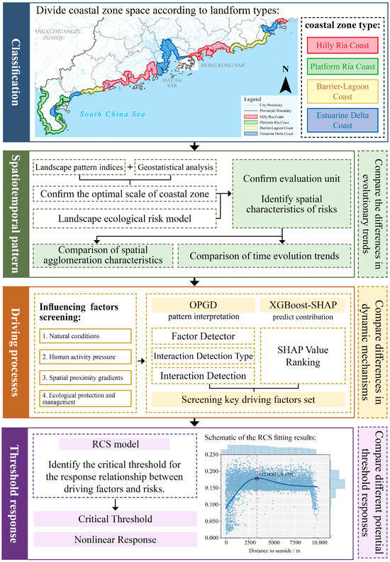
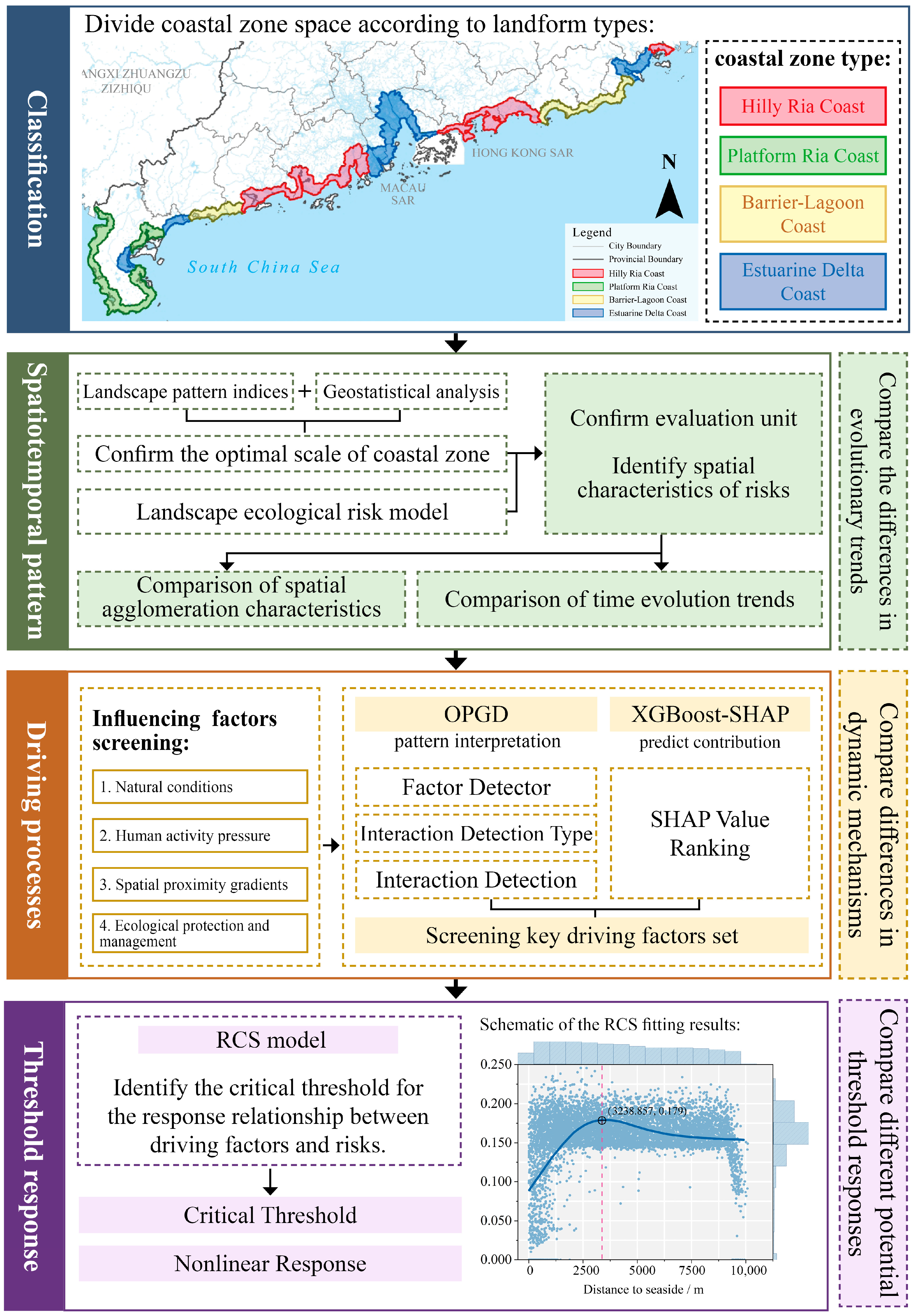
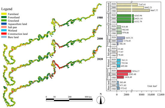
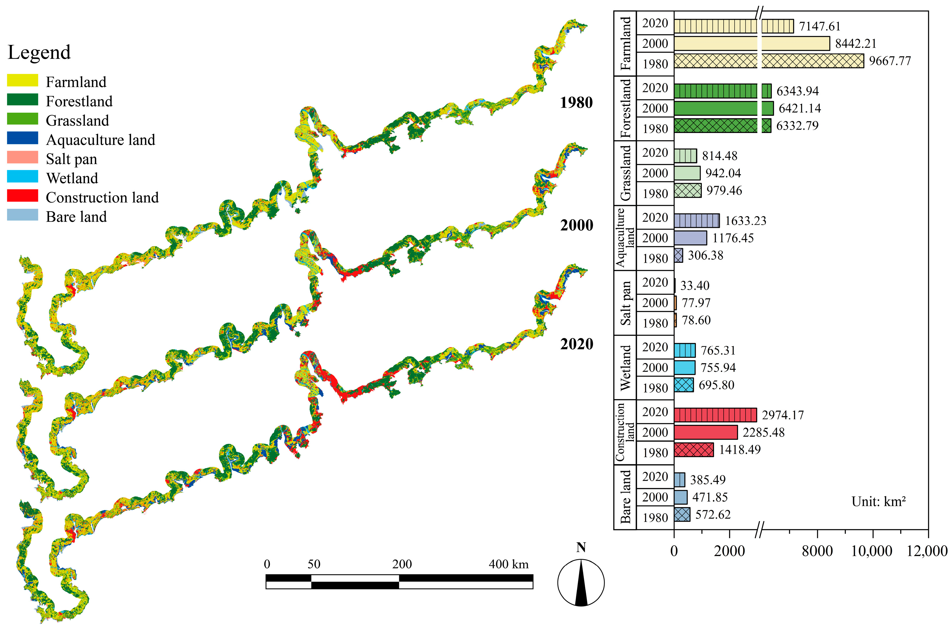
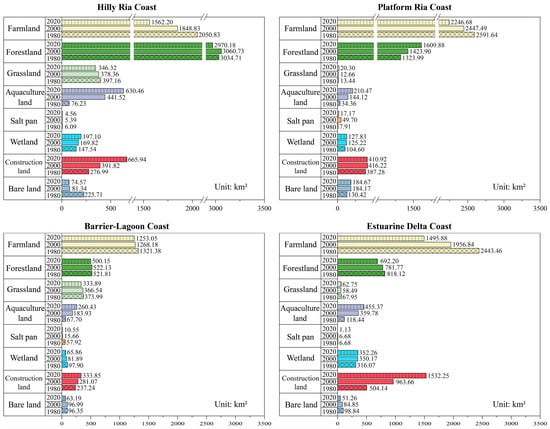
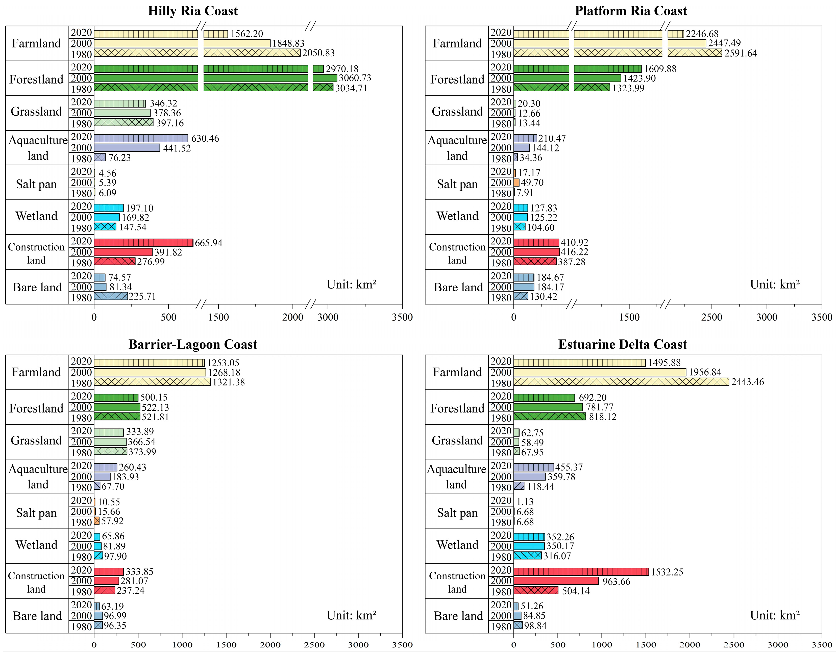
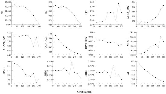
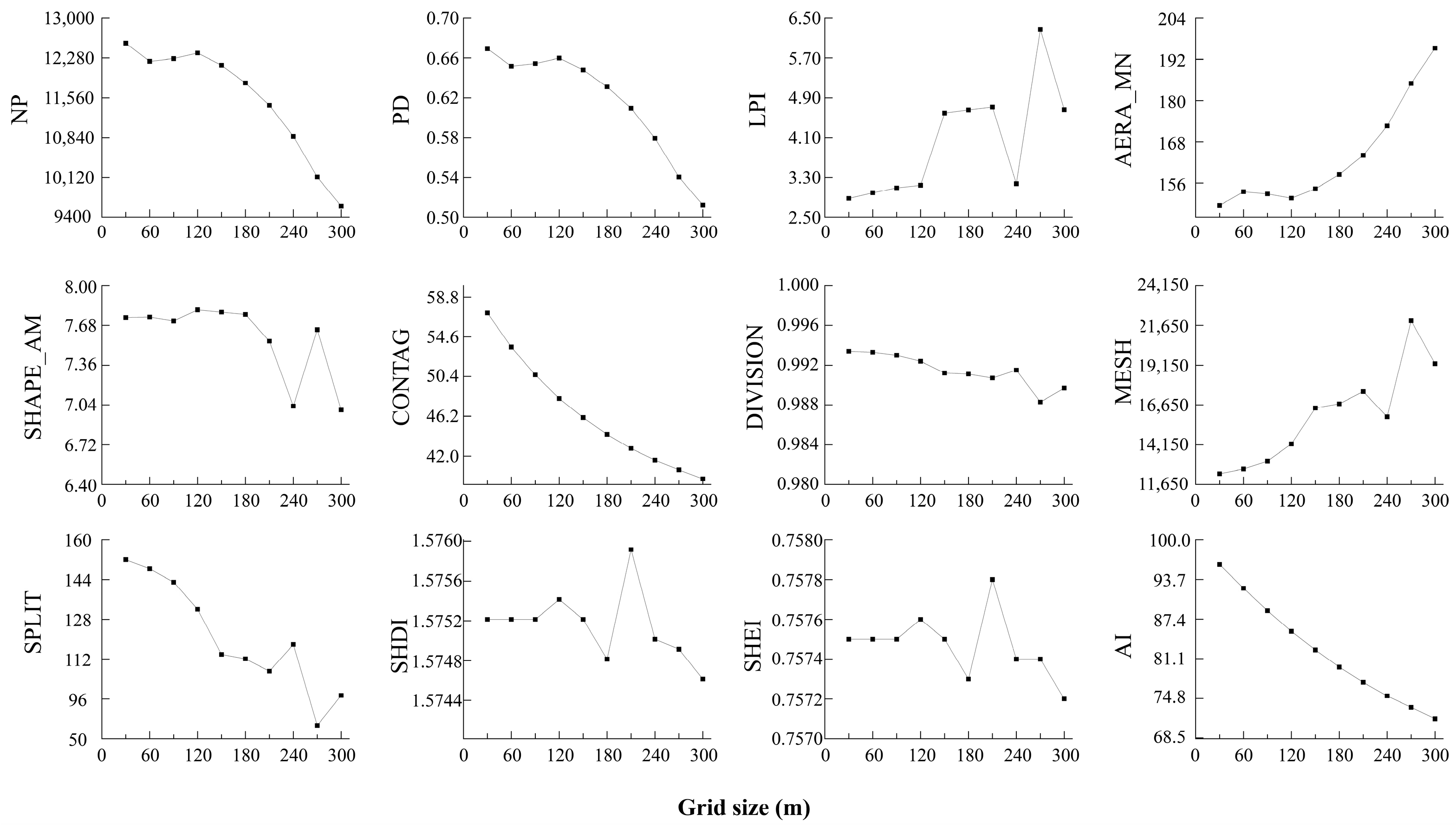
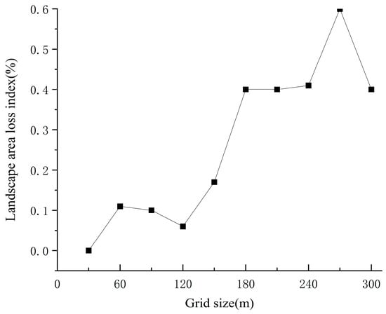
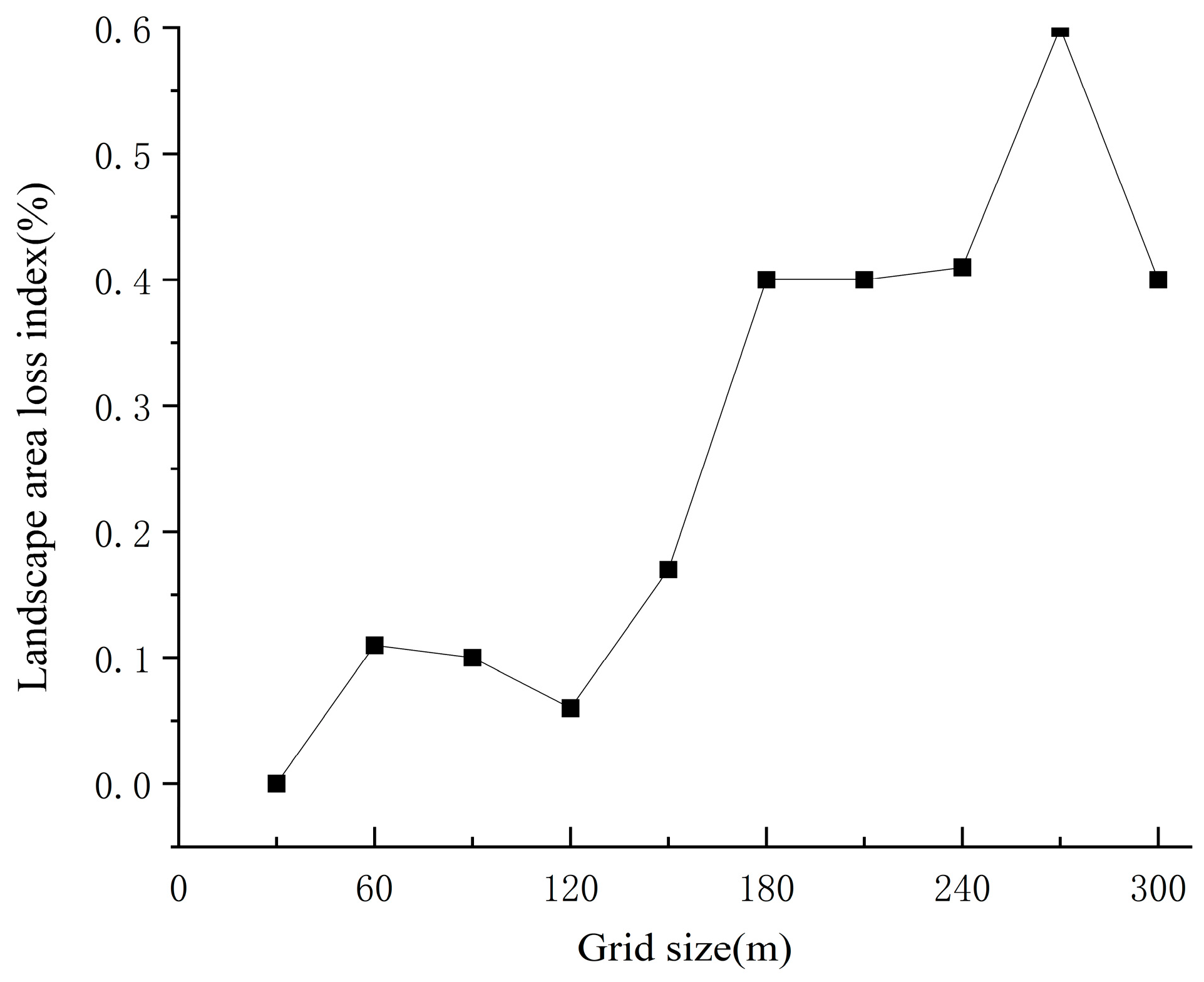
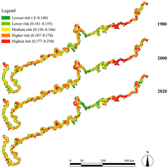
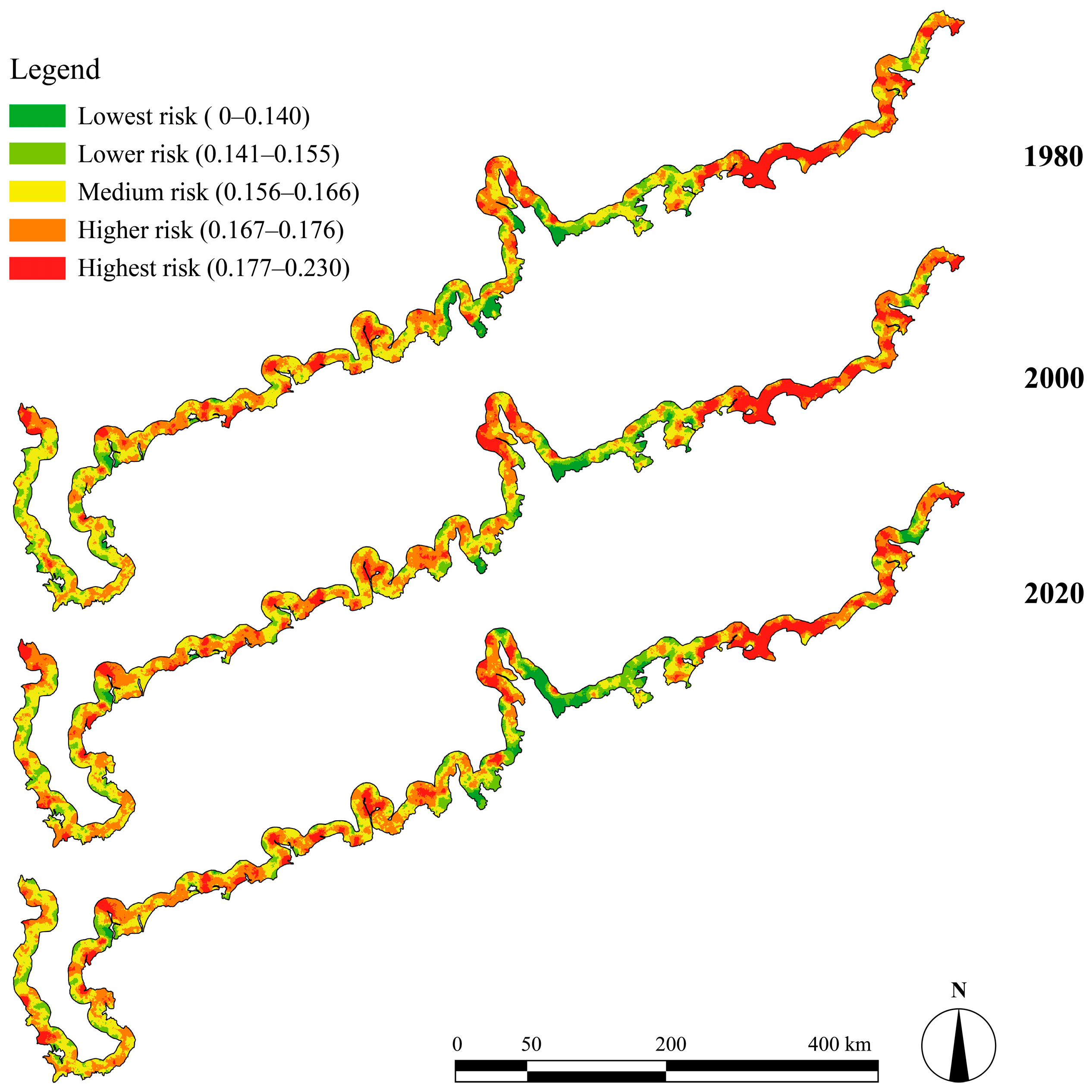
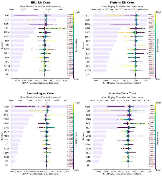
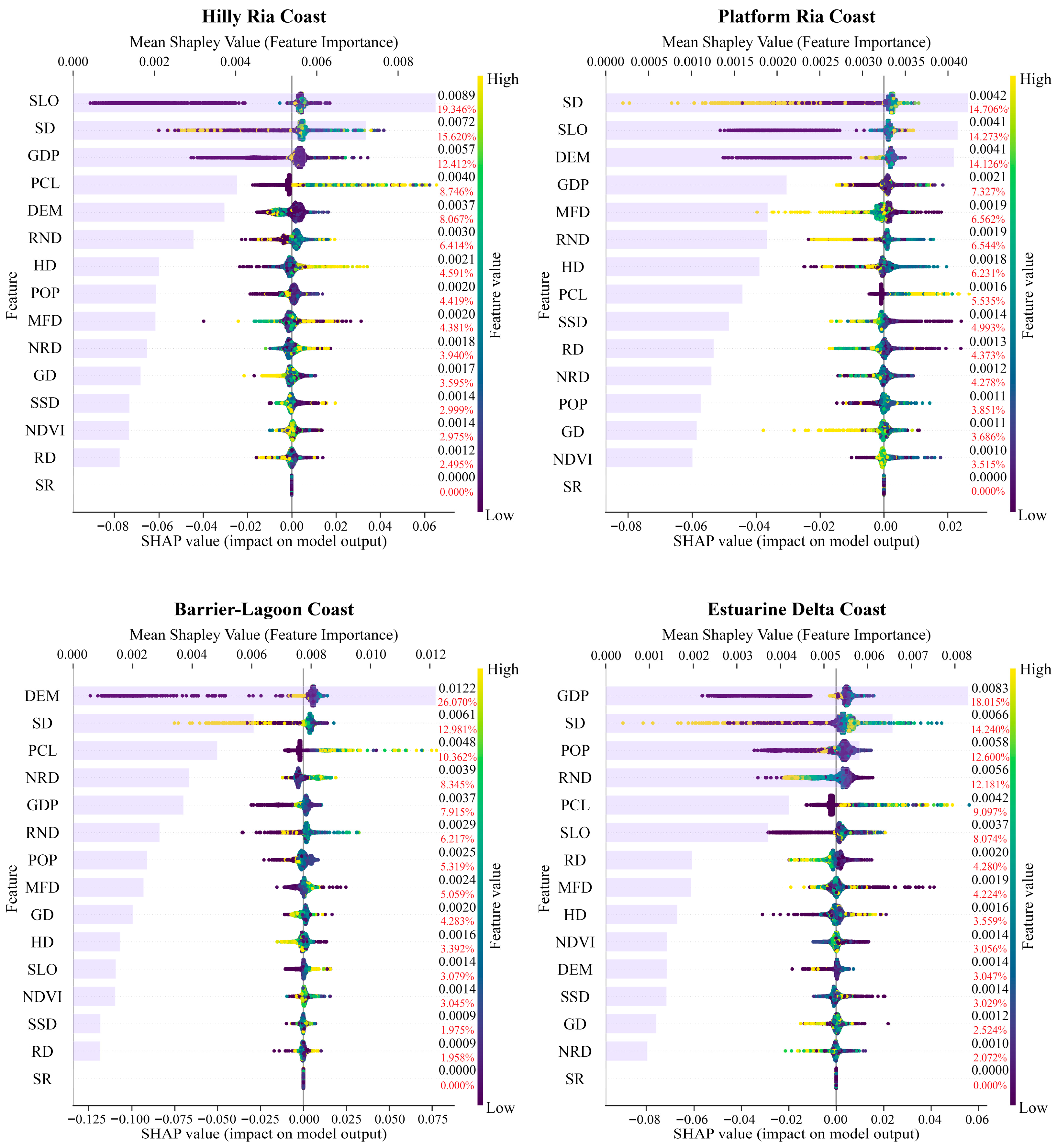
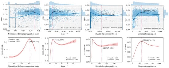
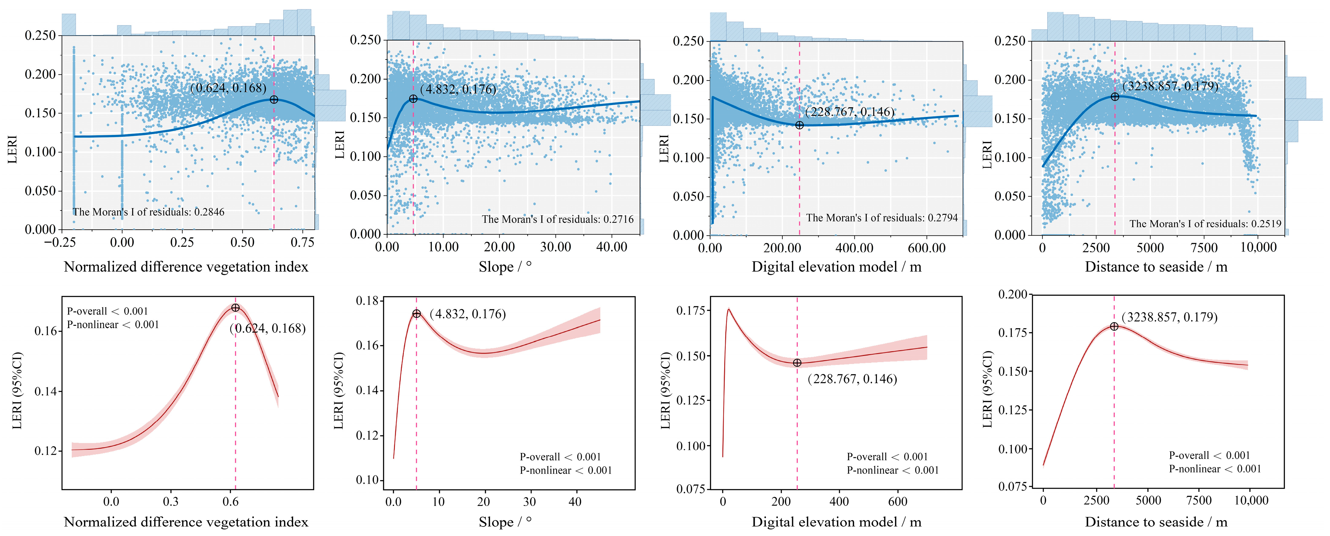
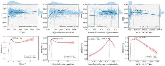
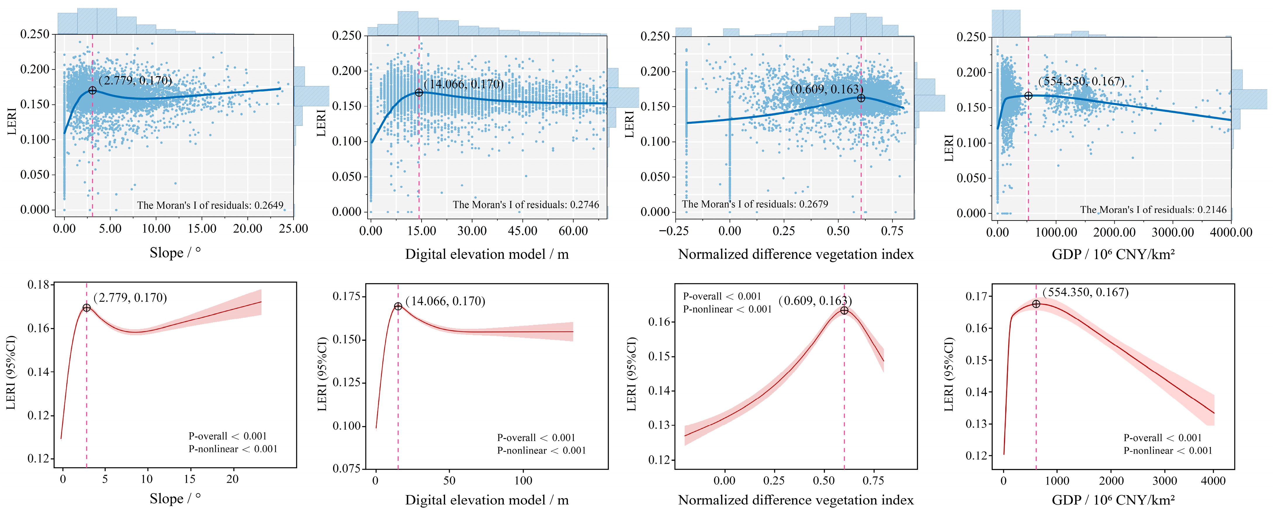
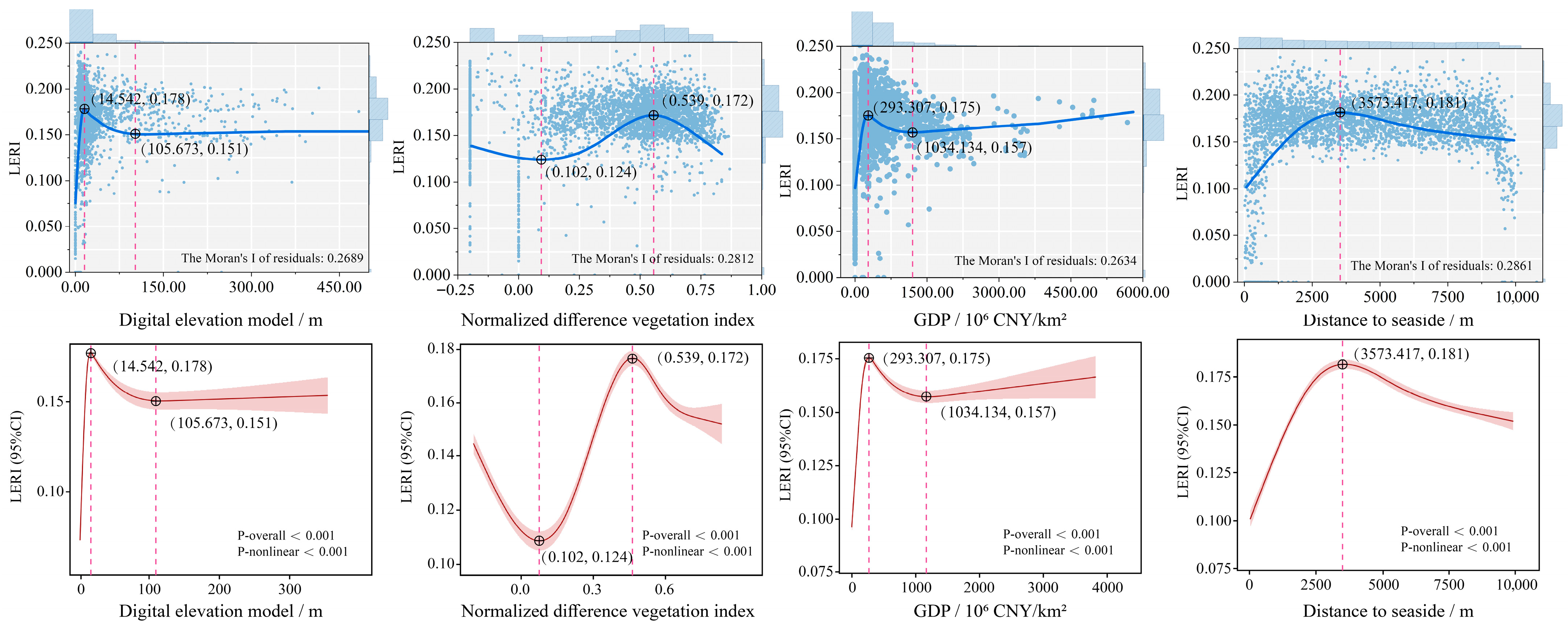
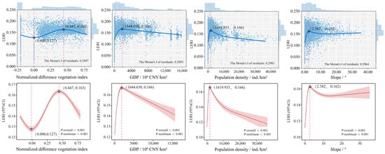
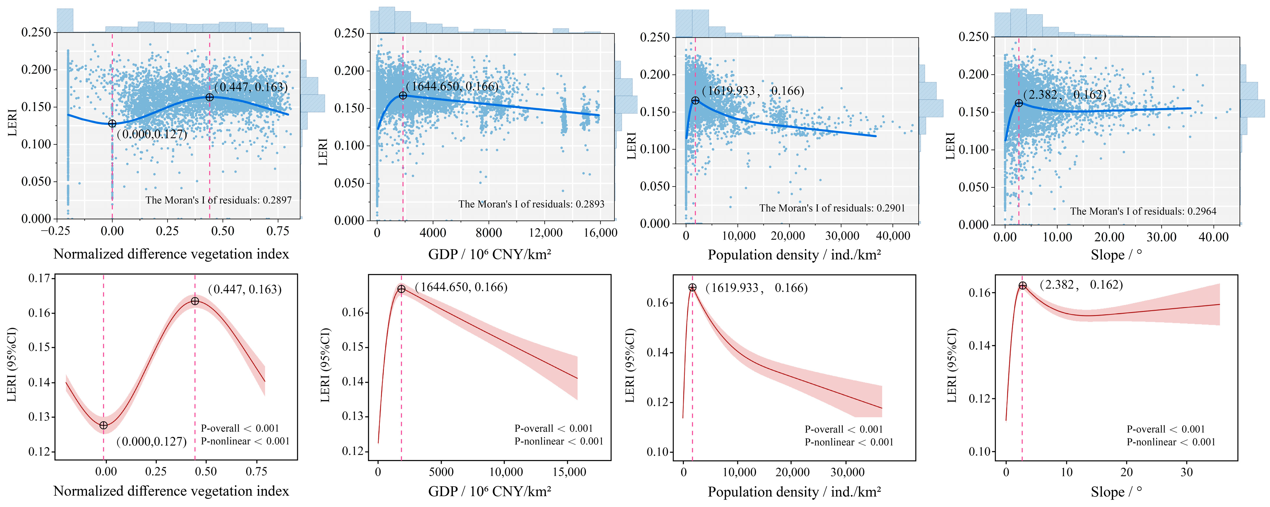

Disclaimer/Publisher’s Note: The statements, opinions and data contained in all publications are solely those of the individual author(s) and contributor(s) and not of MDPI and/or the editor(s). MDPI and/or the editor(s) disclaim responsibility for any injury to people or property resulting from any ideas, methods, instructions or products referred to in the content. |
© 2026 by the authors. Licensee MDPI, Basel, Switzerland. This article is an open access article distributed under the terms and conditions of the Creative Commons Attribution (CC BY) license.