


Abstract
Mapping land cover, monitoring its changes, and simulating future alterations are essential tasks for sustainable land management. These processes enable accurate assessment of environmental impacts, support informed policymaking, and assist in the planning needed to mitigate risks related to urban expansion, deforestation, and climate change. This study proposes a GeoAI-based framework leveraging Multilayer Perceptron (MLP), a class of Artificial Neural Networks (ANNs), to predict land cover changes in the Aosta Valley region (NW Italy). The model uses Copernicus Earth Observation data, specifically Sentinel-1 and Sentinel-2 imagery, and is trained and validated on land cover maps derived from different time periods previously validated with ground truth data. The objective is to provide a predictive tool capable of simulating potential future landscape configurations, supporting proactive regional land use planning including regulatory constraints under the current land use plan. Model performance is evaluated using accuracy metrics. The land cover classification methodology follows established approaches in the scientific literature, adapted to the specific geomorphological characteristics of the Aosta Valley. To explore and visualize potential future land cover transitions, Sankey and chord diagrams are used in combination with zonal statistics and thematic plots. These provide detailed insights into the intensity, direction, and magnitude of landscape dynamics. Training data were stratified-sampled across the study area, covering a diverse set of land cover classes to ensure robustness and generalization of the MLP model. This GeoAI approach offers a scalable and replicable methodology for anticipating land cover dynamics, identifying vulnerable areas, and informing adaptive environmental management strategies at the regional scale, while simultaneously considering the latest urban planning regulations.
1. Introduction
The rapid expansion of Earth Observation (EO) programmes over the past two decades has profoundly transformed the way land surface processes are monitored, analysed, and predicted [1,2,3,4,5]. The increasing availability of high-resolution satellite missions and programmes such as those within the Copernicus, Planets, USGS, and NASA programmes, combined with open-access policies, has enabled unprecedented opportunities for generating detailed land cover and land use maps at a regional and global scale [6,7,8,9]. Sentinel-1 radar data and Sentinel-2 multispectral imagery provide dense temporal coverage and spatial resolutions suitable for capturing fine-scale landscape dynamics, supporting applications ranging from environmental monitoring to territorial planning [10,11,12,13]. As EO archives continue to grow, the challenge is no longer data scarcity but the ability to extract meaningful, actionable information from massive spatiotemporal datasets [14,15,16,17].
In this context, GeoAI, the integration of artificial intelligence techniques with geospatial data and GIS science, has emerged as a transformative paradigm [18,19,20,21,22]. GeoAI encompasses machine learning, deep learning, and spatially explicit modelling approaches tailored to remote sensing and geographic information systems [23,24,25]. Its applications span land cover classification, change detection, object-based image analysis, environmental modelling, and predictive simulation of landscape evolution [26,27,28,29]. By leveraging the computational power of modern hardware and the richness of EO data, GeoAI provides robust tools for forecasting [30,31,32,33] land cover transitions, identifying emerging trends, and supporting evidence-based decision-making [34,35,36,37].
Predictive land change modelling has a long tradition in environmental sciences [38,39,40]. Since the 1980s, Multilayer Perceptron (MLP) and other Artificial Neural Networks (ANNs) have been used within GIS environments to simulate land cover dynamics [41,42,43,44]. However, the true revolution lies in the contemporary convergence of three factors: (i) the exponential increase in freely available satellite data [45,46,47,48,49], (ii) the maturation of open-source geospatial ecosystems [50,51,52,53], and (iii) the availability of high-performance computing resources [54,55]. These advances have enabled more accurate, scalable, and operationally viable predictive models than previously possible [56,57,58]. A variety of open-source tools now support land change simulation workflows [59,60] in GIS tools, enabling transition potential modelling and cellular automaton simulations [61,62,63,64]. While numerous studies have applied GeoAI and MLP-based models [65] to land cover prediction [66,67,68,69], few have explicitly incorporated legal, regulatory, and planning constraints into simulation frameworks [70,71,72,73]. Yet, for territorial planning authorities, predictive models are only meaningful if they reflect the normative context governing land transformation [74,75,76,77]. This includes non-developable areas, ecological protection zones, hazard-prone regions, and municipal land use plans. Integrating such constraints into GeoAI-driven simulations represents a crucial step toward operational, law-compliant predictive tools that can support public administrations in evaluating future development scenarios, assessing policy impacts, and guiding sustainable land management.
The Aosta Valley (NW Italy) provides an ideal testbed for such an approach due to its complex alpine geomorphology, heterogeneous land use patterns, and stringent planning regulations. Its mountainous terrain, characterized by steep altitudinal gradients and extensive high-elevation environments, requires high-resolution spatial data and a wide range of input datasets to develop reliable models. Furthermore, the region is governed by a multilayered regulatory framework that includes hazard zoning maps, landscape protection plans, and municipal master plans, all of which play a crucial role in shaping future land cover trajectories. Integrating such constraints into predictive modelling is essential for producing simulations that are not only scientifically robust but also compliant with real-world planning regulations [78,79,80,81].
Therefore, the main aim of this study is to develop a prototypal system to support future territorial planning by combining Copernicus EO data, MLP-based GeoAI modelling, and regulatory constraints. Specifically, the system aims to: (1) identify vulnerable areas, with particular emphasis on urban expansion, by integrating observed data with planning regulations; (2) map the potential for land cover changes across the entire territory; and (3) provide innovative tools based on GeoAI and satellite data, enhancing existing services [82,83,84] and strengthening digitalization in the geographic and territorial planning domain in the public administration.
The proposed approach offers a replicable and scalable tool for regional planning authorities, environmental agencies, and researchers seeking to anticipate landscape transformations in support of sustainable territorial management. Although the manuscript includes a detailed land cover change analysis, this component is not intended as an end. Rather, it serves as a validation and demonstration of the proposed law-compliant GeoAI framework. The primary contribution of this study lies in the integration of machine learning, cellular automata, demographic drivers, and hierarchical legislative constraints within an operational territorial planning context. Environmental analysis therefore represents an applied case study supporting methodological innovation.
2. Materials and Methods
2.1. Study Area
The study area corresponds to the Aosta Valley (Valle d’Aosta/Vallée d’Aoste), an autonomous region in northwestern Italy located in the heart of the Western Alps. Covering approximately 3263 km2, it is the smallest Italian region by surface area and population, yet one of the most geomorphologically complex territories in Europe (see Figure 1). The region is entirely mountainous, bordered by France to the west, Switzerland to the north, and the Italian region of Piedmont to the south and east. Its landscape is dominated by some of the highest peaks in the Alps, including Mont Blanc (4810 m), Monte Rosa, Matterhorn, and Gran Paradiso, which shape a highly heterogeneous topography characterized by steep altitudinal gradients, narrow valley floors, and extensive high-elevation environments. The Aosta Valley exhibits a remarkable diversity of land cover types, ranging from urban settlements concentrated along the main valley floor to forests, alpine pastures, shrublands, and bare rock at higher elevations. Permanent snow and glaciers occupy significant portions of the upper catchments, contributing to the region’s hydrological and ecological dynamics. This environmental heterogeneity, combined with strong climatic gradients from temperate conditions in the valley bottoms to alpine and nival regimes at higher elevations, makes the region an ideal natural laboratory for studying land cover dynamics using Earth Observation data [85,86].
Figure 1.
The study area involves Aosta Valley Autonomous Region, NW Italy. Map CRS: UTM/ED50 32N (EPSG: 23032).
Human activities are strongly conditioned by geomorphological setting. Urban development is largely confined to limited flat areas, resulting in a linear settlement pattern along the Dora Baltea River corridor. Agricultural land is similarly constrained, with vineyards, orchards, and meadows occupying terraced slopes and valley floors. Tourism, winter sports infrastructure, and hydroelectric facilities represent major drivers of land use change, particularly in high-mountain municipalities. At the same time, large portions of the region fall within protected areas, including the Gran Paradiso National Park and several Natura 2000 sites, which impose strict conservation regulations. From a planning perspective, the Aosta Valley is governed by a multilayered regulatory framework that includes the Piano Territoriale Paesistico (PTP), municipal Piani Regolatori Generali Comunali (PRGC), hazard zoning maps, and sectoral plans for forestry, agriculture, and natural risk mitigation. These instruments define non-developable areas, ecological corridors, and zones subject to hydrogeological or avalanche risk, all of which play a crucial role in shaping future land cover trajectories. Integrating such constraints into predictive modelling is essential for producing simulations that are not only scientifically robust but also compliant with real-world planning regulations.
Demographic dynamics represent a crucial contextual variable for land use and land cover change modelling, particularly in regions where settlement expansion, service demand, and land use pressures are strongly linked to population size and structure. The Aosta Valley, like most Italian regions, is experiencing a long-term demographic decline driven by low fertility rates, population ageing, and a persistent negative natural balance. According to recent ISTAT data, the region has recorded eleven consecutive years of population decrease, with a reduction of 0.1% in 2024 and a cumulative loss of 4.3% of residents since 2014. As of 2023, the resident population stood at 122,877 inhabitants, continuing a modest but steady downward trend [87,88,89,90]. Despite this structural decline, the Aosta Valley shows some distinctive features compared to the national context, particularly regarding birth. While Italy continues to experience record-low birth rates, the Aosta Valley has recently exhibited a slight rebound in births, with a +5.5% increase in the first seven months of 2025, making it one of the few Italian regions to show a positive trend in that period. The regional crude birth rate rose from 3.1‰ in 2024 back to 3.3‰ in early 2025, nearly aligning with the national average of 3.4‰. Although still low in absolute terms, this uptick contrasts with the broader national decline and suggests a slightly more resilient fertility pattern. However, this short-term increase does not offset the long-term demographic contraction. The region continues to face negative natural balance, with deaths exceeding births, which is only partially compensated by internal and international migration flows. The number of births remains historically low, with 641 newborns in 2024, marking the eleventh consecutive year of decline, and fertility remains below replacement level, with an average of 1.05 children per woman (0.98 for Italian women and 1.70 for foreign residents). From a modelling perspective, these demographic trends are relevant because they influence future land use pressures, particularly in valley-floor municipalities where urban expansion is constrained by geomorphology and planning regulations, despite the fact the recovery and activity plan has boosted employment dynamics in the construction and infrastructure sectors (2020–2025), along with trends in tourism demand. Incorporating population dynamics as an explanatory variable helps contextualize potential land cover transitions, especially those related to residential development, service infrastructure, and abandonment of marginal land areas [91,92,93]. In summary, while the Aosta Valley mirrors national patterns of demographic decline, it shows slightly higher or more stable natality levels compared to the Italian average in recent years. Nevertheless, projections indicate that the region will continue to face population shrinkage and ageing, reinforcing the importance of predictive tools for sustainable and regulation-compliant territorial planning.
2.2. Selection Criteria for the Geographic Context
The selection of the Aosta Valley as the study area was motivated by both methodological and substantive considerations. From a methodological perspective, the region represents an ideal testbed for the development and validation of a law-compliant GeoAI framework due to its high geomorphological complexity, strong altitudinal gradients, and the presence of a well-defined hierarchical planning system integrating hazard zoning (P4), landscape protection (PTP), and municipal master plans (PRGC). The coexistence of strict regulatory constraints and spatially heterogeneous land use patterns provides a challenging environment for testing whether predictive models can operate under real legislative admissibility conditions.
From a substantive perspective, the Aosta Valley constitutes a climate-sensitive alpine territory where elevation-dependent ecological shifts, cryospheric retreat, and constrained urban development interact within limited valley-floor areas. This combination makes it particularly suitable for investigating the integration of environmental dynamics and sustainable territorial planning strategies. Furthermore, the availability of high-quality open geospatial datasets through the regional geoportal ensures full reproducibility and operational scalability of the proposed framework.
2.3. Model Input Data and Territorial-Law-Based Constraints
The study focused on the use of land cover maps produced according to a hierarchical approach suitable for complex geomorphological contexts, as described in [94,95]. The maps were derived from Earth Observation data acquired from the Sentinel-2 and Sentinel-1 missions and processed using Google Earth Engine [54], SAGA GIS v. 9.2.0 [51], and RStudio v. 2022.02.2+485 [96,97,98,99,100,101]. These datasets are available for download in vector format or can be requested in raster format at the URL https://geoportale.regione.vda.it/download/carta-copertura-suolo/ (last accessed on 20 January 2026). All input cartographic data are openly accessible and downloadable from the Regional Geoportal of the Aosta Valley (SCT—Sistema delle Conoscenze Territoriali).
The study period covered 2020–2030. Observed input data consisted of biennial land cover maps spanning from 2020 to 2024. To assess the accuracy and robustness of the proposed model, land cover conditions for 2024 were simulated using the 2020 and 2022 maps as inputs, and the observed 2024 land cover map was subsequently employed for validation of the simulated output.
After model calibration, hyperparameters were optimized through the evaluation of accuracy metrics and iterative hyperparameter tuning. The optimal configuration, characterized by high precision and recall as well as low bias and variance, was then selected. Using this calibrated model, temporal simulations were iteratively performed to generate land cover projections for the years 2026, 2028, and 2030. It is worth noting that land cover raster maps were rasterized and reclassified into classes from 1 to 15; each class is reported in Table 1 together with the corresponding codes and acronyms assigned for subsequent analyses. All other datasets were rasterized so that every product shared the same grid structure and the same number of rows and columns. They were then co-registered to ensure perfect pixel-level alignment and temporal consistency across all inputs used in the GeoAI model using the R package ily (https://github.com/ily-R/ImageCoregistration (last accessed on 20 January 2026)).
Table 1.
Land cover legend and acronyms adopted.
Beyond land cover (reported in Figure 2, hereinafter LC) information, several ancillary raster datasets were integrated into the modelling framework to represent topographic, infrastructural, hydrological, and demographic drivers. All datasets were harmonized to a spatial resolution of 10 m to ensure consistency with the LC products.
Figure 2.
Aosta Valley land cover maps for 2020, 2022 and 2024, based on May–September composites (EPSG: 23032).
- (a)
- Topographic variables
A Digital Terrain Model (DTM) derived from LiDAR aerial surveys conducted between 2005 and 2008 was used. The original dataset has a native Ground Sample Distance (GSD) of 2 m and was resampled to 10 m to match the spatial resolution of the LC data. From the resampled DTM, a slope raster was computed using SAGA GIS v. 9.11.0, maintaining a 10 m GSD (both maps shown in Figure 3).
Figure 3.
Aosta Valley DTM and slope maps with a representation scale of 1:350,000. CRS: UTM/ED50 32N (EPSG: 23032).
- (b)
- Hydrological proximity grid (HPG)
Euclidean distance from water surfaces was calculated to represent proximity to hydrological features. Water surfaces included all water bodies and watercourses derived from the water network channel layers available through the regional SCT platform. A proximity grid analysis was performed in SAGA GIS v. 9.11.0, and the resulting raster was produced at a spatial resolution of 10 m (see Figure 4).
Figure 4.
Aosta Valley water surface proximity grid map with a representation scale of 1:350,000. CRS: UTM/ED50 32N (EPSG: 23032).
- (c)
- Transportation network proximity (TNP)
Euclidean distance from the transportation network was derived from mobility network layers obtained from the SCT platform. Like the hydrological analysis, a proximity grid analysis was carried out in SAGA GIS v. 9.11.0, and the output raster was generated at a 10 m GSD (see Figure 5).
Figure 5.
Aosta Valley transportation network proximity grid map with a representation scale of 1:350,000. CRS: UTM/ED50 32N (EPSG: 23032).
- (d)
- Population data
Population density was represented using gridded datasets from the WorldPop project (https://hub.worldpop.org/geodata/listing?id=135 (last accessed on 20 January 2026)). Annual population data covering the period from 2000 to 2030 were compiled from two complementary sources. Population layers up to but not including 2015 were retrieved via Google Earth Engine from the collection ‘ee.ImageCollection (“WorldPop/GP/100m/pop_age_sex_cons_unadj”)’, using the variable *population*. All raster layers were extracted and clipped to the administrative boundaries of the Aosta Valley region, which were obtained in vector format from the regional SCT platform. Population layers for subsequent years (2015–2030) were downloaded directly from the WorldPop repository. WorldPop provides openly accessible, high-resolution demographic datasets designed to support analyses of population dynamics, development planning, and environmental modelling. Population estimates are generated by disaggregating census counts to approximately 100 m grid cells using a Random-Forest-based dasymetric redistribution approach, which exploits relationships between population density and multiple geospatial covariates. The datasets used in this study correspond to top-down constrained estimates, in which national population totals are adjusted to match official United Nations figures (UN DESA, World Population Prospects 2019). Further methodological details and validation procedures are documented in the project’s peer-reviewed literature. All native 100 m population layers were resampled to 10 m to ensure consistency with the spatial resolution of the other geospatial inputs used in the modelling framework. Each annual raster was then processed to extract pixel-wise temporal trends over the full 2000–2030 period. For each pixel, a linear regression model was fitted to estimate the gain (slope), offset (intercept), and trend significance. The resulting gain map, representing the long-term rate of population change, was subsequently used as an input variable in the GeoAI model. For each pixel, the temporal evolution of population values over the 2000–2030 period was modelled using a simple linear regression of the following form (see Equation (1)):
where:
P(t) is the population value at year t;
β0 is the offset (intercept);
β1 is the gain (slope, i.e., annual rate of change);
ε is the residual error term.
Specifically, the terms of Equation (1) are explained in Equations (2) and (3).
The statistical significance of the temporal trend was assessed using the Mann–Kendall non-parametric test, which is appropriate for monotonic trends, non-normally distributed data, time series with potential outliers, and environmental and geospatial datasets. The Mann–Kendall statistic S is defined as follows (Equation (4)):
with the standardized test statistic (Equation (5)):
A trend is considered statistically significant when (Equation (6)):
with Za/2 typically equal to 1.96 for a 95% confidence level.
The maps of gain, offset, p-value, and determination coefficient are shown in Figure 6 below.
Figure 6.
Aosta Valley population density gain, offset, p-value and R2 from first-order polynomial modelling of 2000–2030 trends (WorldPop data; CRS UTM/ED50 32N, EPSG: 23032).
It is important to note that the gain layer was treated as an optional variable. Two sets of simulations were therefore produced for the 2024–2030 period: one based on the complete set of baseline covariates, and a second including all variables together with the population-gain layer. This approach made it possible to evaluate how the explicit inclusion of population dynamics influenced the model’s behaviour and outputs.
Beyond the above-mentioned datasets, a map was generated considering urban planning restrictions. Urban planning constraints were derived from the following datasets: non-buildable areas (“Ambiti inedificabili—Hazard zones P4”), the most recent legally valid municipal master plan (“Piano Regolatore Generale Comunale”, PRGC), and the landscape territorial plan (“Piano Territoriale Paesistico”, PTP). All datasets are publicly available at the following URL: https://geoportale.regione.vda.it/ (last accessed on 20 January 2026).
The cartographic layers were spatially harmonized and rasterized to define the constraints to be integrated into the GeoAI model, following a rule-based approach grounded in territorial development regulations. Specifically, non-buildable areas were assigned the highest priority, followed by the landscape territorial plan (PTP), and finally by the municipal master plan (PRGC). These priority rules constitute the core of the rule-based framework adopted for the creation of the input constraint mask supplied to the model.
It should be noted that, within the Italian planning system, the PRGC must always comply with the PTP and Ambiti P4, which is hierarchically superior from a regulatory standpoint and whose provisions must be incorporated into municipal planning instruments. Consequently, from a cartographic perspective, higher-priority layers spatially override subordinate layers through polygon overlap. The final constraint product is therefore harmonized with the highest-priority planning layer, ensuring consistency with the normative hierarchy governing territorial planning. In order to summarize these regulation rules, a table has been provided (see Table 2).
Table 2.
Hierarchy of planning instruments and regulations in the Aosta Valley, Italy.
Below, the territorial constraint map obtained considering the above-mentioned criteria (reported in Table 1) is depicted (see Figure 7). It is worth noting that non-buildable areas fall within P4 hazard zones or within areas subject to non-modifiable constraints as defined by the currently valid PTP and PRGC. Conversely, potentially buildable areas are in zones that do not currently fall within hazard areas or non-modifiable constraints but are assigned other land use designations or restrictions that could potentially be changed, allowing future development. Examples include grassland areas without current risk conditions that are not presently buildable but are located near an urban core, or areas subject to stringent constraints (e.g., cultural heritage or historical protection, or park reserves) that could become developable only after specific authorization procedures.
Figure 7.
Aosta Valley territorial constraint map obtained considering the regulations reported in Table 1. Representation scale of 1:350,000; CRS: UTM/ED50 32N (EPSG: 23032).
In the future scenario model, a rule was introduced whereby all spaces classified as buildable areas are filled first, and only subsequently are potentially buildable areas considered. Figure 8 shows the municipalities equipped with complete planning instruments approved by the Regional Authority as of 2025, as well as those lacking approved or up-to-date validated plans.
Figure 8.
Municipalities of the Aosta Valley region with complete planning instruments approved by the Regional Authority as of 2025, and municipalities without approved or updated validated plans. Representation scale of 1:350,000; CRS: UTM/ED50 32N (EPSG: 23032).
It should be emphasized that, for the three municipalities with planning data that are not updated or formally approved, reference was made to the most recent draft planning instrument available, together with the regional constraints defined by the PTP and the related zoning frameworks. Consequently, in these areas the model may be more strongly affected by biases related to uncertainty in local planning instruments.
2.4. GeoAI Prototypal Model
Land use and land cover (LULC) changes were modelled using the Modules for Land Use Change Simulations (MOLUSCE) plugin implemented in QGIS, developed by Asia Air Survey and NextGIS (https://github.com/nextgis/qgis_molusce (last accessed on 20 January 2026)). MOLUSCE is a GeoAI-based modelling framework that integrates spatial drivers, transition analysis, and machine learning algorithms to simulate future land use dynamics under predefined constraints; it is quite similar to Land Changer Modeler in TerrSet IDRISI software from Clark Labs [64,102,103,104].
In its standard configuration, MOLUSCE estimates the probability of transition between land cover classes by learning from historical land cover changes and a set of explanatory spatial variables, primarily biophysical and accessibility-related drivers (e.g., slope, elevation, and proximity to urban centres). Transition probabilities are then used to generate future land use scenarios through spatial allocation rules, neighbourhood effects, and stochastic processes.
Specifically, in this study, the open-source Python v. 3.12 code of MOLUSCE was extended to:
- (a)
- Explicitly integrate legislative planning constraints as hard rules for areas designated as urban and anthropic areas;
- (b)
- Introduce population density and trends as mandatory, dominant drivers for transitions toward urban and anthropic areas;
- (c)
- Maintain the original MOLUSCE logic for all other land cover classes.
Land cover transitions were modelled using an Artificial Neural Network (ANN), specifically a feed-forward Multilayer Perceptron (MLP), as implemented in MOLUSCE. The MLP architecture consists of an input layer, a hidden layer, and an output layer, with unidirectional information flow, from inputs to outputs (see Equations (7)–(10)). Let
be the vector of normalized explanatory variables for each pixel. The output of a neuron j in the hidden layer is computed as:
where indicates synaptic weights, is the bias term, and is a sigmoid activation function:
The output layer estimates the transition probability for each land use transition class k as:
where indicates the hidden-to-output weights, is the output bias, and m is the number of hidden neurons.
To ensure regulatory compliance, hard constraints were applied exclusively to transitions toward the urban and anthropic areas class. For all other land cover classes, the original MOLUSCE logic governs transitions, including neighbourhood effects and biophysical drivers.
Let denote a land cover class, and let denote the set of urban and anthropic areas (see Equations (11) and (12)). The class-specific constraint function is defined as:
The effective transition probability is therefore:
This ensures that urban and anthropic areas cannot expand into legally non-buildable zones, while all other land cover transitions remain unconstrained and follow the standard MOLUSCE rules (Equation (13)).
where:
represents legislative admissibility;
represents population density or trend;
represents biophysical drivers (e.g., slope, elevation, etc.).
A weighted input transformation was applied to enforce hierarchical importance (Equations (14) and (15)):
with
where are the weight coefficients that define the relative importance of each driver.
The resulting class-specific transition probability is therefore as follows (Equation (16)):
In the case of population density, its modelled trend, when included as an explanatory variable for transitions toward urban and anthropic areas, followed the pattern described below.
In this case, population acts as a secondary dominant driver only for urban and anthropic areas, while biophysical and neighbourhood effects govern transitions of other classes.
The ANN was trained using supervised learning by minimizing the mean squared error (MSE) between observed and predicted transitions (see Equation (A1) in the Appendix A). Weight updates were performed using gradient descent with momentum (see Equation (A2) in Appendix A).
Optimal ANN hyperparameters were identified through an extensive hyperparameter tuning procedure, consisting of ~5,000,000 simulation runs. A randomized grid-search strategy was used to explore the hyperparameter space and select the configuration that minimized validation error while avoiding overfitting. The following ranges were explored:
- -
- Learning rate, ;
- -
- Momentum, ;
- -
- Number of hidden neurons, ;
- -
- Maximum iterations, ;
- -
- Training sample size, .
The best-performing ANN configuration was:
- -
- Learning rate: ;
- -
- Momentum: ;
- -
- Maximum iterations: 3000;
- -
- Hidden layer size: 10 neurons;
- -
- Stratified training samples: 20,000;
- -
- Training/validation split: 60%/40%.
Below are the learning curves of the neural network during training for both modelling configurations, with (Figure 9) and without (Figure 10) the inclusion of the population-gain driver.
Figure 9.
Learning curves of the neural network during training. The plot shows the evolution of the loss function across training iterations for both training and validation datasets, illustrating progressive optimization and stabilization of the error as the model converges, considering population gain as input.
Figure 10.
Learning curves of the neural network during training. The plot shows the evolution of the loss function across training iterations for both training and validation datasets, illustrating progressive optimization and stabilization of the error as the model converges, without considering population gain as input.
The explanatory variables related to land cover dynamics were initially selected based on a comprehensive review of the scientific literature and empirical evidence identifying the main drivers of land cover change [41,75,105,106,107,108]. This preliminary selection ensured that all candidate predictors were conceptually meaningful and relevant to the processes under investigation. Subsequently, prior to model implementation, the selected explanatory variables were examined for multicollinearity using the Pearson correlation coefficient. This screening step ensured that redundant or highly collinear variables did not distort the learning process of the Artificial Neural Network (ANN). Therefore, pairwise correlations were calculated among all predictors to assess the degree of linear dependence. Variables exhibiting high correlation values were generally considered redundant and excluded from the analysis to avoid biasing the learning process of the Artificial Neural Network. Only variables showing low-to-moderate correlation levels were retained, ensuring that the final set of predictors provided largely independent information to the modelling framework. As illustrated in Figure 11, the only highly correlated variables retained in the model are TNP and HPG. This exception is justified by the geomorphological characteristics of the study area, where transportation infrastructures are predominantly developed along hillslopes and valley floors near hydrological networks. Such spatial patterns reflect the geological processes that have shaped the alpine landscape, resulting in an intrinsic relationship between road networks, hydrographic features, and terrain morphology. In fact, in the model, the transition potential for each land cover class is first estimated through the ANN (a feed-forward Multilayer Perceptron), which learns from historical LC changes and the selected spatial drivers. The resulting probability surfaces represent the intrinsic suitability of each cell to undergo a specific transition according also the rules included.
Figure 11.
Pearson correlation matrix of selected land cover change predictors, used to assess linear associations and limit multicollinearity. Light blue indicates weaker correlations, with increasing brightness reflecting stronger relationships. Circles oriented from the lower left to upper right denote positive trends (as indicated by the coefficient values), whereas those from the upper left to lower right indicate negative trends. Most variables show low–moderate correlations; a strong correlation occurs only between TNP and HPG, retained due to the study area’s geomorphology.
These transition potentials are then spatially allocated using a cellular automaton (CA) approach. As reported in Equation (17), a CA consists of: (a) a grid of cells, (b) a neighbourhood (e.g., Moore 3 × 3), and (c) a transition rule.
For each cell , the CA update rule can be expressed as:
where:
= new state of cell ;
= ANN transition potential;
= neighbourhood effect at time ;
= constraint factor (1 = allowed, 0 = forbidden);
= transition threshold.
The neighbourhood term typically increases when adjacent cells already belong to the target class, thus modelling spatial contiguity and diffusion, typical of urban expansion and other land use processes in case of the absence of the constraint factor. CA models operate on a discrete raster grid where each cell can change state according to: (a) its transition potential, (b) the states of neighbouring cells, and (c) predefined evolution rules. This mechanism introduces neighbourhood effects, such as spatial contiguity, clustering, and diffusion, that are typical of real land cover dynamics (e.g., urban expansion tends to occur adjacent to existing built-up areas). The CA component therefore transforms the non-spatial ANN probabilities into spatially coherent future land cover patterns. Specifically, the final transition potential surface used for allocation is computed by combining ANN outputs, neighbourhood effects, and constraints as reported in Equation (18):
where:
= final transition potential;
= calibration parameters controlling the influence of suitability vs. neighbourhood;
= hard constraints (e.g., legally protected areas and planning restrictions).
Cells with higher are more likely to undergo transition during the CA allocation process.
2.5. Model Performance and Accuracy Metrics
The performance of the model was evaluated by comparing the simulated land cover (LC) map with the reference LC map for the year 2024. A set of widely used accuracy metrics derived from the confusion matrix were employed to assess the predictive capability and robustness of the model. The confusion matrix quantifies the agreement between simulated and observed LC classes by identifying true positives (TPs), true negatives (TNs), false positives (FPs), and false negatives (FNs) at the pixel level. The following metrics have been computed: overall accuracy (OA), precision, recall, F1-score, and Cohen’s kappa () (see Equations (A4)–(A8) in Appendix A). Finally, a flowchart summarizing the main inputs, processing steps, and outputs of the workflow is provided in Figure A1 (see Appendix A).
3. Results
The results presented below serve a dual purpose: (i) to assess the predictive accuracy and robustness of the GeoAI framework, and (ii) to evaluate whether the integration of hierarchical territorial constraints produces spatially coherent and regulation-compliant outputs. Therefore, emphasis is placed not only on environmental dynamics but also on model behaviour under planning rules. In land cover change modelling, prediction outputs can be expressed through soft and hard predictions, which differ in terms of representation, interpretation, and level of information provided. In both LC modelling configurations adopting and not adopting the population-gain driver, maps were produced for the years 2024 (validated against the reference dataset), 2026, 2028, and 2030. These outputs are referred to as soft prediction (SP) and hard prediction (HP), respectively.
SP represents the probability of change for each spatial unit (e.g., pixel or cell) and is typically expressed on a continuous scale ranging from 0 to 100 (or 0–1). This value indicates the likelihood that a land cover change will occur, without directly assigning a specific land cover class. Low values correspond to a minimal probability of change, while high values indicate a maximum probability of transition. Soft predictions preserve uncertainty and are particularly useful for identifying areas more susceptible to transformation, supporting risk assessment and scenario analysis.
On the other hand, HP is derived from SP by applying decision rules or thresholds. It produces a discrete land cover map, where each spatial unit is assigned to a specific class according to a predefined legend. The assignment is based on the probabilities estimated in the soft prediction and on transition rules that determine which classes the land cover migrates from and to. For example, a pixel classified as meadow or pasture in the initial map may be reassigned to urbanized or anthropogenic area in the hard prediction, depending on the highest transition probability and the imposed constraints.
In this framework, soft prediction answers the question of “where change is more likely to occur”, while hard prediction defines “what change will occur and into which land cover class”. Together, they provide a comprehensive representation of land cover dynamics, combining probabilistic information with explicit spatial classification suitable for planning, scenario simulation, and policy evaluation. Figure 12 and Figure 13 report, respectively, the soft prediction (SP) and hard prediction (HP) maps generated without and with the inclusion of the population-gain driver. Specific zoomed-in focus maps are shown in Figure S1 onwards in the Supplementary Materials.
Figure 12.
Comparative soft prediction (SP) maps for 2024–2030: (upper part) model configuration excluding population-gain driver; (lower part) model configuration including population-gain driver.
Figure 13.
Hard prediction (HP) maps for 2024–2030: (upper part) model configuration excluding population-gain driver; (lower part) model configuration including population-gain driver. Map legend is the same as in Figure 2.
The performance evaluation highlights the strong and consistent ability of the model to simulate land cover (LC) changes under both configurations, with and without the inclusion of population gain as an input driver (metrics obtained in Table 3).
Table 3.
Model performance with and without population gain as input driver.
In the configuration excluding population dynamics, the model achieved an overall accuracy of 0.83 when comparing the simulated LC map with the reference map for 2024. The agreement analysis confirms the robustness of this configuration: the overall model kappa reached 0.81, indicating a strong level of agreement beyond chance, while the model kappa of 0.80 suggests that the ANN effectively captured land cover transition processes. The small difference between these indices indicates stable learning behaviour and no evidence of overfitting. From a transition detection perspective, the model achieved a recall of 0.78, indicating a good capacity to identify actual LC changes, although some omission errors remain. The precision value of 0.87 reflects a limited proportion of false-positive transitions, highlighting the relatively conservative behaviour of the model in predicting change. The resulting F1-score of 0.82 confirms a balanced trade-off between omission and commission errors. When population gain was included as an input driver, the model performance improved across all metrics. The overall accuracy increased to 0.86, calculated by comparing the simulated LC map with the reference map for 2024. The agreement analysis further supports the robustness of this configuration, with an overall model kappa of 0.85 and a model kappa of 0.84, both indicating strong agreement beyond chance and confirming the model’s capability to represent land cover transition processes. The minimal difference between the two indices again suggests stable learning behaviour and no evidence of overfitting. In terms of change detection, the model achieved a recall of 0.81, demonstrating a good ability to identify actual LC changes. Although some omission errors persist, the precision value of 0.90 indicates a very low proportion of false-positive transitions, confirming the conservative nature of the model when predicting change. The resulting F1-score of 0.85 reflects a well-balanced trade-off between omission and commission errors and further supports the reliability of the simulation. The overall accuracy could potentially be higher; however, it is partially constrained by the misclassification of snow-covered pixels in 2024, a year characterized by an unusually long persistence of snow cover. The model is inherently influenced by the input land cover datasets, which in this case correspond to the 2020 and 2022 observations and therefore reflect average climatological conditions. Consequently, the model is able to reproduce long-term land cover dynamics but is less effective in capturing short-term meteorological anomalies affecting specific years. Although both modelling configurations produced robust results, the inclusion of population gain yielded higher accuracy values and outputs that better represent territorial dynamics relevant to land cover management and spatial planning. For this reason, the analysis of class migration was conducted using the HD outputs generated with the population gain driver. These outputs not only achieved the highest accuracy statistics but also exhibited greater physical and socio-spatial coherence with the observed territorial processes, which could not be fully captured by the configuration excluding demographic trends despite its acceptable statistical performance.
Land Cover Changes and Future Trends
All land cover transitions were quantified using the OpenLand R package v. 1.0.3 [109,110], which produced category-level gains and losses, transition intensities, chord diagrams for each interval, a multi-step Sankey diagram, and a cumulative transition map [111,112,113,114,115] for the full period (2020–2030). It is worth noting that changes in urban and anthropogenic areas (Uaa) strictly follow the planned development rules and occur only in areas where such transitions are allowed, including population dynamics, as previously reported. The simulation results reveal a spatially structured and directionally coherent pattern of land cover transformation over the 2020–2030 period. Hard prediction outputs (Figure 13) indicate that changes are not randomly distributed but are concentrated primarily in high-elevation zones, while valley floors and forested mid-elevation belts remain largely stable. At the landscape level, the dominant process is the progressive expansion of bare rock/soil, accompanied by the contraction of natural grasslands and alpine pastures and, to a lesser extent, snow and ice (see Figure 14). Gross and net change analysis (Figure A2, Figure A3, Figure A4 and Figure A5 in Appendix A) confirms this directional system: Bare rock/soil exhibits the largest net gain, while natural grasslands and alpine pastures represent the main source category. Snow and ice also show consistent net losses, though involving smaller absolute areas. Importantly, these transitions are characterized by strong asymmetry, with limited swapping processes and a clear prevalence of unidirectional flows. Urban and anthropic areas show only moderate net expansion, occurring exclusively within legally admissible zones as defined by the hierarchical constraint mask implemented in the modelling framework. A Sankey diagram has been reported in Figure 15. The cumulative change map (Figure 16) further confirms that transformation processes are spatially clustered, particularly in exposed alpine environments, while forest systems, especially needle-leaved forests, demonstrate high persistence and structural stability. This spatial differentiation reinforces the internal consistency of the model outputs and their alignment with geomorphological and climatic gradients. Detailed category-level and transition-level intensity analyses, including multi-step Sankey flows and one-step chord diagrams, are provided in Figure A2, Figure A3, Figure A4 and Figure A5 in Appendix A to support the robustness and transparency of the modelling results. Quantitative analysis of land cover (LC) class areas reveals a structurally persistent landscape configuration over the 2020–2030 period, with three classes collectively accounting for most of the mapped extent. Bare rock and soil (Brs) represented the dominant LC class throughout the entire time series, exhibiting a statistically consistent net areal gain from approximately 800–900 km2 in 2020 to over 1100 km2 by 2030, with the rate of increase intensifying post-2024. Needle-leaved forests (Ndf) maintained a stable extent of 500–600 km2, with no discernible directional trend. Natural grasslands and alpine pastures (Ngp) underwent a progressive and substantial areal reduction, declining from approximately 600–800 km2 in 2020–2022 to 300–400 km2 by 2030. All remaining classes individually contributed less than 100–300 km2 and displayed negligible interannual variability.
Figure 14.
Temporal evolution of land use/land cover (LUC) areas from 2020 to 2030. Stacked bar plot showing the area (in km2) occupied by each of the 15 reclassified LUC categories across annual time steps from 2020 to 2030.
Figure 15.
Sankey diagram illustrating multi-step land cover transitions from 2020 to 2030. Node heights and ribbon widths represent category areas and transition magnitudes (km2), respectively. Vertical flows indicate persistence, while horizontal ribbons depict inter-category changes. Colours follow the reclassified LUC legend (Table 1).
Figure 16.
Cumulative land cover change map for the period 2020–2030. Grey: no change detected (persistence in the same category across all intervals). Red: changed at least once during the decade. The map highlights the spatial concentration of transitions, primarily in high-elevation zones.
Multi-temporal flow analysis identifies Ngp-to-Brs conversion as the primary transition pathway, consistently representing the largest inter-category flux across all two-year intervals throughout the decade. Secondly, persistent flow corresponds to cryospheric retreat (Gsi to Brs), contributing cumulatively to bare substrate expansion. Urban and anthropic areas (Uaa) exhibited a moderate but directionally consistent net gain, sourced predominantly from adjacent herbaceous classes (Ngp, Dhvmla, and Shvha), with negligible reverse transitions, indicative of an irreversible low-intensity anthropogenic encroachment process. Forest classes (Ndf, Blf, and Mfm) displayed characteristically high self-transition rates, with minimal inter-category outflows, confirming their structural stability within the landscape matrix (for more detail, see Figure 15).
Finally, spatial analysis of cumulative change over the full study period reveals a strongly non-random distribution of transitional pixels (see Figure 16). Changed areas are preferentially clustered in high-elevation zones, along alpine ridges and transitional slopes, consistent with the topographic and ecological gradients governing Ngp contraction and Gsi retreat, and the corresponding Brs expansion. Stable pixels dominate mid-elevation forested sectors and valley floors, in accordance with the high persistence coefficients of Ndf and other woodland classes. Dispersed transitional pixels at lower elevations spatially correspond to the incremental Uaa expansion identified in the categorical and flow analyses. Collectively, the spatial pattern corroborates a climatically mediated, elevation-dependent regime shift in the alpine and subalpine belt, with anthropogenic land conversion remaining spatially confined and limited in regional magnitude.
Overall, the cumulative change map confirms that the decade was characterized by localized but substantial transformation rather than uniform landscape-wide turnover. Change was concentrated in high-altitude, open, and exposed environments, where grassland contraction and cryospheric retreat drove exposure of bare substrates. In contrast, forested, lower-elevation, and anthropically modified areas remained predominantly stable, with only limited encroachment by urban/anthropic classes against low vegetated surfaces. This spatial pattern underscores a climatically mediated elevation-dependent shift in the alpine and subalpine belt, with minimal evidence of widespread anthropogenic land conversion at the regional scale according to the territorial planning rules.
4. Discussion
The analyses conducted for the 2020–2030 period reveal a coherent and strongly convergent pattern of land cover transformation, dominated by a directional expansion of bare substrates at high elevations. This increase occurred primarily at the expense of natural grasslands and alpine pastures, which experienced the largest net losses, and of snow and ice, which also declined substantially. These transitions constitute the principal axis of change throughout the decade, whereas anthropogenic expansion remained limited in both magnitude and spatial extent. Transition-level intensity metrics and flow diagrams consistently show that land cover change followed highly targeted pathways. The most intense and persistent transition was from natural grasslands and alpine pastures to bare rock and soil, exceeding uniform intensity expectations in every interval. This pathway was reinforced by sustained transitions from snow and ice to bare substrates, which, despite involving smaller absolute areas, displayed high relative intensity. Spatially, these changes were concentrated in exposed high-elevation environments ridges, plateaus, and upper slopes forming extensive interconnected zones of transformation, while lower valleys, forested mid-elevation belts, and topographically sheltered slopes remained largely stable. The elevation-dependent nature of these dynamics aligns with climate-driven processes commonly observed in mountain regions undergoing warming. Accelerated snow and ice melt, longer snow-free periods, upward shifts of vegetation belts, and potential permafrost degradation collectively reduce grassland and cryospheric cover while exposing rocky surfaces. The marked deceleration of change intensity after 2024 may reflect a saturation effect, with diminishing areas available for conversion, or interannual variability in climatic drivers influencing melt rates and vegetation responses. Needle-leaved forests emerged as the most stable land cover class, exhibiting strong persistence, balanced gross gains and losses, and extensive continuity across mid-elevation zones. Their resilience likely reflects lower thermal sensitivity relative to alpine grasslands, the protective influence of topographic sheltering, and the inherently slow pace of treeline dynamics. Other forest types and most agricultural or semi-natural classes showed minimal involvement in transition processes [116,117,118]. Urban and anthropogenic areas displayed only modest net expansion, largely confined to valley bottoms and accessible slopes, and sourced mainly from adjacent herbaceous covers [119,120,121]. Although small in magnitude compared with high-elevation transformations, this trend remains relevant in mountain contexts where infrastructure development, tourism facilities, and localized urban sprawl can encroach upon limited natural or semi-natural land [122,123]. While the elevation-dependent shifts observed in alpine grasslands and cryospheric areas are consistent with regional climate trends, the core contribution of this work lies in demonstrating how such processes can be simulated within a legally constrained planning framework. The integration of hard legislative masks ensures that predictive expansion of urban and anthropogenic areas remains fully compliant with hazard zoning and landscape protection rules, a feature rarely addressed in conventional land change modelling studies.
The study successfully met its three primary aims outlined in the introduction. First, the integration of observed data, planning regulations, and open-source tools enabled the identification of vulnerable areas, particularly with respect to urban expansion. Second, the model effectively mapped the potential for land cover changes across the entire territory, as demonstrated by the spatial and temporal analyses. Third, the development of an innovative GeoAI-based tool using satellite data has enhanced existing services and strengthened digitalization in geographic and territorial planning within public administration. The extended GeoAI modelling framework enriched with territorial constraints and population-gain trends represents a significant methodological advancement. By integrating regulatory, demographic, and environmental drivers into a unified predictive system, the model translates normative requirements into operational geospatial layers, guiding non-generative AI through explicit, transparent rules. This is particularly relevant for public administrations, which increasingly require decision-support tools capable of aligning Earth Observation-based analyses with planning regulations and governance needs. The prototype developed here fulfils this objective, offering a replicable, scalable tool for regional planning authorities, environmental agencies, and researchers.
The hierarchical driver integration assigns the highest weight to legislative constraints (λleg), followed by population trends (λpop), and finally biophysical variables (λbio). This structure reflects real-world planning: urban expansion can only occur where legally permitted; among admissible areas, demographic pressure determines the likelihood of conversion; and within demographically suitable zones, biophysical factors influence final spatial allocation. Population gain interacts with distance to transportation networks (TNP): areas with positive demographic trends near existing infrastructure show higher transition probabilities toward Uaa than predicted by either variable alone. Conversely, in areas with negative population trends, even favourable biophysical conditions do not result in urban expansion, explaining why the model with population gain achieves higher precision by avoiding false positives in depopulating areas.
The model is highly adaptable and scalable, allowing the introduction of new constraints or favourable/unfavourable conditions depending on planning objectives. It generates complementary outputs: soft prediction maps expressing probabilistic transition potentials and hard prediction maps providing deterministic forecasts, which together support comprehensive scenario analysis and risk assessment. Built on open-source tools and well-documented algorithms, the system avoids the opacity typical of many generative AI approaches, ensuring transparency essential for public, auditable, and regulation-compliant decision-making.
Despite its strengths, the model presents several limitations [124,125,126]. It requires substantial expertise in remote sensing, GeoAI, and programming, as well as high-performance computing resources, especially when processing high-resolution datasets [127,128,129]. Although Copernicus provides free 10 m data, achieving sub-metre resolution often depends on commercial sources, which may limit accessibility. The model also faces structural constraints when deriving high-definition predictions from limited temporal observations, due to the absence of recurrent architectures such as Long Short-Term Memory (LSTM) networks. Furthermore, the model’s performance can be affected by interannual meteorological anomalies, as seen in the misclassification of snow-covered pixels in 2024 [130,131,132,133,134,135,136,137,138,139,140,141,142]. Specifically, the misclassification of snow-covered pixels in 2024 reveals both a limitation and an opportunity. While the model cannot capture interannual meteorological variability when trained on average conditions (2020–2022), it successfully identifies areas where snow persistence deviates from historical patterns. This anomaly highlights the need for future model iterations to integrate climate projections as dynamic drivers. Incorporating temperature and precipitation scenarios would enable simulation of land cover trajectories under different climate futures, particularly for climate-sensitive transitions such as Gsi to Brs and Ngp to Brs, which are likely to accelerate under warming scenarios in alpine environments. Contrary to what global accuracy metrics alone might suggest, the model performs robustly in low-altitude areas and regions with significant human activity, though this performance is expressed differently than in high-elevation environments. While high-elevation transitions (Ngp to Brs and Gsi to Brs) are characterized by large areal extent and climate-driven dynamics, urban expansion in valley bottoms is intentionally constrained by the hierarchical legislative rules embedded in the framework. The overall accuracy of 0.86 and kappa of 0.85 demonstrate strong regional performance that includes low-altitude areas. However, the evaluation of urban simulation quality must consider the following factors: (a) Hard constraints prevent illegal expansion: Unlike high-elevation transitions, which follow biophysical suitability, urban expansion can only occur where legally permitted. This means the model correctly predicts no change in vast low-altitude areas subject to P4 hazard zones or landscape protection, representing a successful application of the law-compliant framework rather than a limitation. (b) Population dynamics improve precision where change is allowed: Within legally buildable areas, the inclusion of population gain ensures that urban transitions are predicted only where demographic pressure supports development. This explains the improved precision (from 0.87 to 0.90) when population is included: the model avoids false-positive urban predictions in buildable-but-depopulating areas. (c) Urban extent is naturally limited: The modest spatial extent of urban areas (∼50–100 km2 over the decade, compared to >500 km2 for Brs) means that even small absolute errors can affect class-specific metrics. However, this reflects the geomorphological reality of the Aosta Valley (narrow valley floors and extensive protected areas) rather than model inadequacy. The model’s behaviour in low-altitude areas is therefore not a weakness but a deliberate design feature: it prioritizes regulatory compliance and demographic realism over purely data-driven expansion. Future work will integrate very-high-resolution validation data (e.g., municipal cadastral maps) to assess urban simulation quality at the parcel level, but the current framework already demonstrates that urban predictions are spatially coherent, legally admissible, and demographically plausible.
Looking ahead, several avenues for improvement and expansion are evident. The integration of GeoAI-based super-resolution techniques could enhance Sentinel-2 imagery from 10 m to sub-metre scales, enabling finer classification and more detailed simulations. Incorporating LSTM or similar temporal deep learning architectures would improve the model’s ability to capture long-term dependencies and complex temporal dynamics. Additionally, future versions should introduce constraints for forest classes to distinguish between natural dynamics, legal management, and illegal logging, while carefully preserving the model’s capacity to detect natural disturbances such as windthrow or climate-induced dieback [143]. The explicit inclusion of population-gain trends represents a step forward, but further demographic and socio-economic variables could be integrated to refine anthropogenic change projections [144,145,146].
The strong agreement across analytical levels’ net and gross change, category- and transition-level intensities, temporal trajectories, and spatial patterns supports the robustness of the findings and the model’s utility for evidence-based planning. The expansion of bare substrates at high elevations carries significant implications for ecosystem services, including reduced forage availability, diminished soil carbon storage, increased erosion, and heightened geomorphic risks [147]. From a conservation perspective, the contraction of alpine grassland habitats may threaten specialist species and endemic biodiversity. The model’s ability to simulate these changes under regulatory constraints offers a proactive tool for designing adaptive management strategies, supporting sustainable territorial planning, and enhancing resilience in mountain regions undergoing rapid environmental change.
Beyond the empirical findings, the study demonstrates the potential of an extended GeoAI modelling framework enriched with territorial constraints and population-gain trends. The model integrates regulatory, demographic, and environmental drivers into a unified predictive system, enabling the translation of normative requirements into operational geospatial layers that guide non-generative AI through explicit, transparent rules. This is particularly relevant for public administrations, which increasingly require decision-support tools capable of aligning Earth Observation-based analyses with planning regulations and governance needs. The prototype developed here aims precisely at this objective: a GeoAI system applied to Earth Observation data that encodes clear, rule-based constraints and supports territorial planning by identifying areas potentially vulnerable to future transitions, providing predictive modelling based on EO data and GeoAI, and assisting public authorities in drafting new plans and monitoring possible interventions.
The modelling framework was further strengthened by the application of downscaled Copernicus data, refined from 10 m to 1 m ground sampling distance. This enhancement significantly improved spatial detail, enabling more accurate delineation of fine-scale features and more precise identification of areas with high transition potential. The demonstration available at https://gamayos.github.io/gamma-earth-api/s2dr3-demo-20250305.html?ds=IT-T32TLR-306c3d4f8-20250818#13.65/45.73716/7.32385 (last accessed on 25 January 2026) illustrates how high-resolution EO data can be integrated into a scalable GeoAI pipeline. This capability is particularly valuable in mountainous regions, where micro-topographic variability strongly influences land cover dynamics and where coarse-resolution datasets may fail to capture critical patterns. The extension of the model to incorporate population-gain trends represents another methodological advancement. Demographic pressure is a key driver of land take in valley bottoms and peri-urban areas, and its explicit inclusion allows the system to better represent the likelihood of anthropogenic expansion. Future work should also introduce constraints for forest classes, ensuring that the model can distinguish between natural forest dynamics, legal forest management, and illegal logging. Care must be taken, however, to avoid over-constraining the system in ways that suppress genuine natural processes such as windthrow, bark beetle outbreaks, or climate-induced dieback. A balanced approach is required to preserve the model’s ability to detect both anthropogenic and natural drivers of forest change. The GeoAI model presents several advantages. It is highly scalable and adaptable to specific territorial needs, allowing the introduction of new constraints or favourable and unfavourable conditions depending on planning objectives. It generates two complementary outputs: soft prediction maps, which express probabilistic transition potentials, and hard prediction maps, which provide deterministic forecasts. The system is based on open-source tools and algorithms within the extensive scientific literature, avoiding the opacity typical of many generative AI approaches. This transparency is essential for public administrations, which require traceable, auditable, and regulation-compliant decision-support systems. However, some limitations must be acknowledged. The model requires substantial expertise in remote sensing, GeoAI, and programming, as well as high-performance ICT resources, especially when working with high-resolution datasets. Although Copernicus provides free 10 m data, achieving sub-metre resolution typically requires commercial sources, which may not always be accessible. The model also faces structural limitations when producing high-definition predictions from a small number of temporal observations, due to the absence of recurrent architectures such as Long Short-Term Memory networks. Incorporating LSTM or similar temporal deep learning models in future developments could improve the system’s ability to capture complex temporal dependencies. It is important to preserve the distinction between observed data (pre-2024) and modelled hard prediction outputs (post-2024), ensuring that the interpretation of results remains consistent with the underlying data sources. Despite these methodological considerations, the strong agreement across analytical levels’ net and gross change, category- and transition-level intensities, temporal trajectories, and spatial patterns supports the robustness of the findings. The expansion of bare substrates at high elevations has important implications for ecosystem services, including reduced forage availability, diminished carbon storage in grassland soils, increased surface erosion, and heightened risk of rockfall or debris flows. From a conservation perspective, the contraction of alpine grassland habitats may negatively affect specialist species and endemic flora and fauna adapted to cryosphere–grassland ecotones. Overall, the decade was characterized by a climatically mediated transformation of high-elevation landscapes, marked by the systematic replacement of vegetated and cryosphere covers with bare substrates. Mid-elevation forests and lower valleys remained comparatively stable, while anthropogenic expansion was limited. The integration of GeoAI modelling, high-resolution EO data, and regulatory constraints demonstrates the potential of advanced spatial decision-support systems to enhance territorial planning, improve vulnerability assessment, and support public administrations in developing adaptive strategies for mountain environments undergoing rapid environmental change. The framework is designed to be scalable, but its transfer to other contexts requires several adaptation steps. For different geographic areas, the explanatory variables must be recalculated using locally available datasets. If LiDAR data are not available for deriving topographic variables such as DTM and slope, global elevation models can be used, although with lower accuracy. Proximity variables can be generated from commonly available vector layers such as hydrographic and road networks, while global datasets such as WorldPop or similar sources can provide population information. After preparing the new inputs, predictor variables should be checked for multicollinearity to ensure their statistical independence. Adapting the model to other regulatory frameworks requires redefining the hierarchy of spatial constraints according to local planning systems. This involves identifying the legal precedence of planning instruments, converting regulatory boundaries into raster layers consistent with the model resolution, and defining constraint functions that determine whether land cover transitions are permitted or restricted. The hierarchical structure of the model allows additional regulatory levels to be incorporated when necessary. The framework can also operate under different data conditions because the modelling architecture is not tied to a specific spatial resolution. Although the current implementation uses Sentinel-1 and Sentinel-2 data at 10 m resolution, alternative datasets such as Landsat can be used where optical coverage is limited, radar-only approaches can be applied in persistently cloudy regions, and super-resolution techniques can improve spatial detail. When applying the model to new datasets, training sample size and hyperparameters should be recalibrated, although the same optimization strategy can be maintained. Extending the forecasting horizon beyond the current 2030 projection would require incorporating dynamic drivers such as climate projections and demographic scenarios rather than static variables or simple trends. In addition, longer historical time series would improve calibration and increase the reliability of long-term simulations. Finally, testing the framework in different geographic and regulatory contexts is essential for assessing its generalization capacity. Ongoing applications in other European regions suggest that the GeoAI architecture itself transfers well, but the hierarchy of regulatory constraints must be carefully adapted to local planning systems. These considerations clarify how the framework can be transferred and provide guidance for future implementations in different territorial contexts.
5. Conclusions
The results obtained for the 2020–2030 period demonstrate that the proposed modelling framework can produce spatially coherent and statistically robust land cover change simulations while ensuring full compliance with hierarchical territorial planning regulations. The predictive performance achieved (overall accuracy up to 0.86; kappa 0.85 when including population trends) confirms the reliability of the GeoAI–cellular automaton integration for medium-term scenario generation. From an environmental perspective, the simulations highlight a strongly directional transformation process concentrated in high-elevation environments. The dominant transition from natural grasslands and alpine pastures to bare rock/soil, together with the progressive retreat of snow and ice, suggests elevation-dependent dynamics consistent with regional climatic trends. These patterns were spatially clustered and not randomly distributed, reinforcing the internal coherence of the model outputs. Forest systems, particularly needle-leaved forests, exhibited high persistence and structural stability, while urban and anthropic areas showed only moderate expansion. However, the primary contribution of this study lies not in the descriptive analysis of these dynamics per se, but in demonstrating how such processes can be simulated within a legally constrained and operational territorial planning framework. By explicitly integrating P4 hazard zones, the landscape territorial plan (PTP), and municipal master plans (PRGC) as hierarchical hard constraints, the modelling architecture ensures that transitions toward urban and anthropic areas occur exclusively where legally admissible. This approach moves beyond conventional land change modelling by embedding regulatory admissibility directly into the transition probability structure, thereby bridging the gap between predictive environmental modelling and real-world governance. The inclusion of demographic trends as a dominant driver for urban transitions further enhances the socio-spatial realism of the simulations. The improvement in predictive metrics when incorporating population gain confirms the relevance of demographic dynamics in shaping land transformation processes within constrained alpine territories. Importantly, the framework demonstrates scalability and replicability. All input datasets derive from openly accessible Copernicus Earth Observation products and regional geoportals, and the modelling pipeline relies on open-source tools. This ensures transferability to other mountainous or regulation-intensive regions where planning compliance represents a central constraint for land development. Overall, the study provides a prototypal GeoAI system capable of supporting public administrations in scenario evaluation, vulnerability mapping, and forward-looking territorial governance. Rather than offering a purely descriptive land cover assessment, the work proposes an operational decision-support architecture in which environmental dynamics, demographic drivers, and legislative hierarchies are integrated within a unified modelling environment. Such integration represents a necessary step toward digitally enabled, regulation-aware territorial planning in the context of climate change and socio-demographic transition. Future developments may include the integration of climate projections, dynamic hazard evolution scenarios, and uncertainty quantification modules to further enhance the decision-support capacity of the framework.
Supplementary Materials
The following supporting information can be downloaded at: https://www.mdpi.com/article/10.3390/land15040533/s1.
Author Contributions
Conceptualization, T.O.; methodology, T.O.; software, T.O. and D.C.; validation, T.O. and D.C.; formal analysis, T.O.; investigation, T.O.; resources, T.O. and D.F.; data curation, T.O.; writing—original draft preparation, T.O.; writing—review and editing, T.O.; visualization, T.O. and D.C.; supervision, T.O. and D.F.; project administration, T.O.; funding acquisition, T.O. and D.F. All authors have read and agreed to the published version of the manuscript.
Funding
This specific research received no external funding, but it has been developed within the framework of the funds of the National Recovery and Resilience Plan (PNRR Italy), “PROGETTO BANDIERA”, and enhancement of the digital capacity of the regional public administration (PNC) (CUP: B71F23000330001) for the development of a prototypal GeoAI system based on open-source data and libraries for the predictive mapping of land cover to support spatial planning, based on the integration of local GIS data and Earth Observation data for the autonomous region of the Aosta Valley (Italy).
Data Availability Statement
Data can be accessed by a formal request to the corresponding author, authorized by INVA spa and the Aosta Valley region according to all the regulations. The data and other information including codes can be requested by e-mail, and the request will be evaluated according to INVA spa rules.
Acknowledgments
During the preparation of this manuscript/study, the authors used Anthropic Claude, Copilot, DeepSeek and Grok last versions in January 2026 for the purposes of coding support and improving the quality of the manuscript. The authors have reviewed and edited the output and take full responsibility for the content of this publication. We would like to thank INVA spa, the Aosta Valley autonomous region and Raffaele Rocco for this opportunity. We also express our sincere gratitude to Annalisa Viani.
Conflicts of Interest
All authors were employed by the company INVA spa. The authors declare that the research was conducted in the absence of any commercial or financial relationships that could be construed as a potential conflict of interest.
Appendix A
Formulas
The ANN was trained using supervised learning by minimizing the mean squared error (MSE) between observed and predicted transitions (Equation (A1)):
where:
is the loss function (mean squared error);
is the total number of training samples;
is the observed land use transition for sample (1 if the transition occurred, 0 otherwise);
is the ANN-predicted transition probability for sample .
Weight updates were performed using gradient descent with momentum (Equation (A2)):
where:
is the weight update at iteration ;
is the learning rate, controlling the step size in weight updates;
is the gradient of the loss function with respect to weight ;
is the momentum coefficient, which adds a fraction of the previous weight update,
, to stabilize convergence.
For two variables and , the Pearson coefficient is defined as follows (Equation (A3)):
Values close to indicate strong correlation, while values near indicate weak or no linear association.
Overall accuracy (OA) represents the proportion of correctly classified pixels out of the total number of pixels (Equation (A4)):
This metric provides a general measure of model correctness but does not account for agreement occurring by chance.
Precision quantifies the reliability of the model in predicting a given class and is defined as follows (Equation (A5)):
Recall measures the model’s ability to correctly identify actual land cover transitions (Equation (A6)):
The F1-score represents the harmonic mean of precision and recall, balancing omission and commission errors (Equation (A7)):
Cohen’s kappa () was used to evaluate the agreement between simulated and observed maps while accounting for random agreement (Equation (A8)):
where:
is the observed agreement (overall accuracy);
is the expected agreement due to chance.
Two kappa indices were considered:
Overall model kappa, assessing the global agreement of the simulation;
Model kappa, focusing on transition dynamics captured by the ANN.
Flowchart summary
Flowchart summary of the methodology adopted with inputs, processing, and outputs.
Integrated summary of land cover change dynamics (2020–2030)
Overall, the combined evidence from Figure A2, Figure A3, Figure A4 and Figure A5 indicates a targeted, climatically mediated transformation of high-elevation environments, primarily driven by the conversion of alpine vegetation and cryospheric land covers into bare substrates, accompanied by limited anthropogenic expansion and a progressive reduction in overall landscape change intensity throughout the decade. The temporal trajectory shows an early peak in change intensity (2020–2022) followed by a progressive deceleration of landscape turnover toward the end of the study period.
Category-level dynamics (Figure A2)
Bare rock and soil (Brs) exhibits the largest absolute gains (approximately 100–250 km2 yr−1) and the highest net increase, although relative gain intensities generally remain close to the uniform threshold, indicating expansion proportional to the class’s large baseline area rather than anomalously accelerated change. Natural grasslands and alpine pastures (Ngp) represent the primary source category, with persistent losses (≈30–80 km2 yr−1) and loss intensities frequently exceeding the uniform line, identifying Ngp as the class undergoing the most active contraction relative to its extent. Snow and ice (Gsi) also display elevated relative loss intensities despite limited absolute areas, consistent with progressive cryospheric retreat. Needle-leaved forests (Ndf) remain largely stable, while minor herbaceous classes show modest contractions, and some minor categories (e.g., Uaa, Wdc, and Wc) register small proportional gains.
Figure A1.
Flowchart illustrating the main stages of the processing workflow, including inputs, intermediate processing steps, and final outputs.
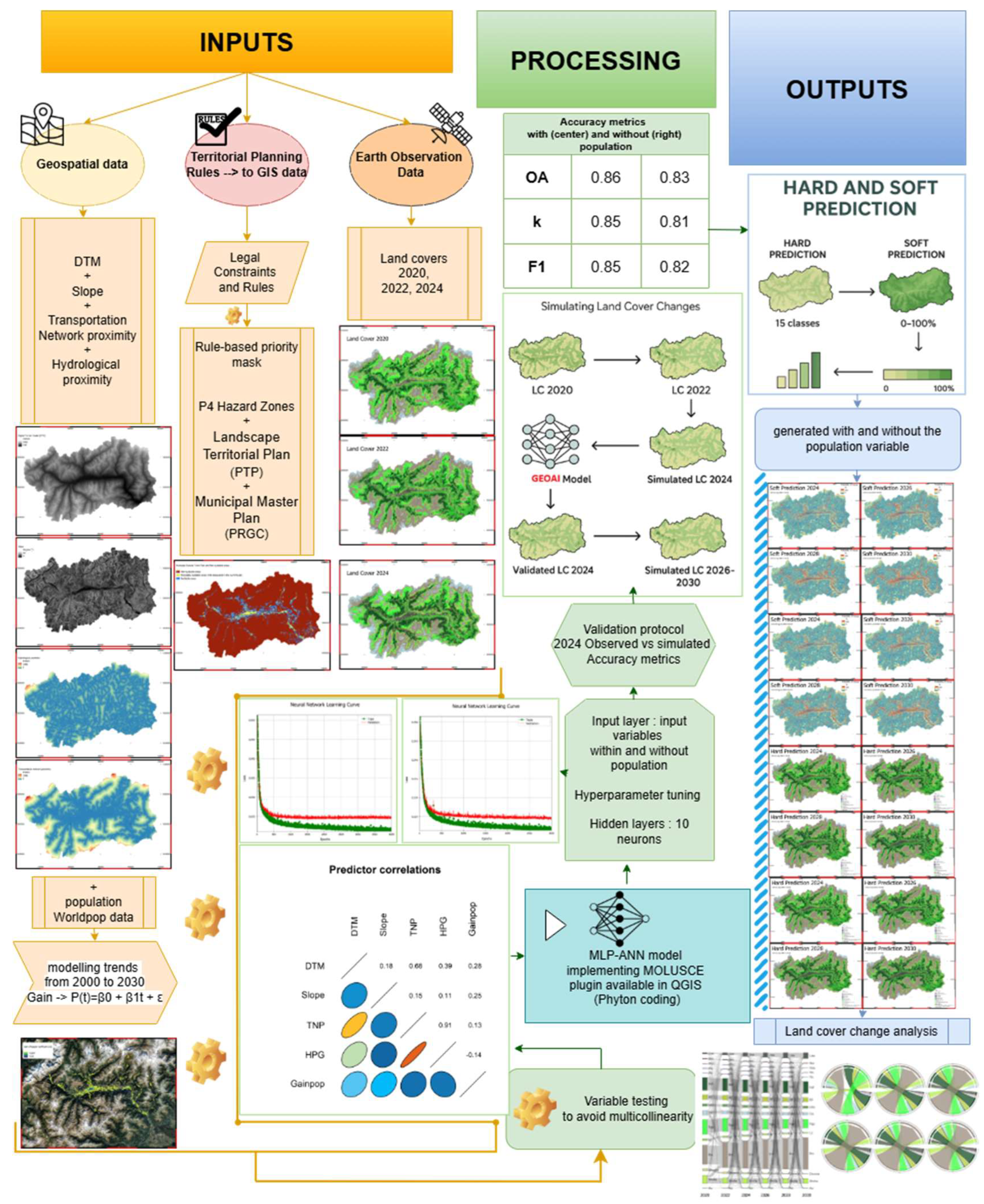
Transition-level intensity of land cover change (2020–2030) (Figure A3)
Transition-level intensity analysis reveals a highly selective pattern dominated by two pathways. The transition of Ngp to Brs constitutes the principal landscape flux, consistently recording the largest annual areas (≈50–120 km2 yr−1) and relative intensities substantially exceeding the uniform transition threshold. A secondary but ecologically meaningful pathway is Gsi to Brs, reflecting the progressive exposure of rocky substrates following snow and ice retreat. All other transitions are comparatively minor. Forest classes show negligible inter-category exchanges, while urban and anthropic areas (Uaa) receive limited inflows primarily from herbaceous covers.
Figure A2.
Category-level intensity analysis of land cover change for consecutive two-year intervals from 2020 to 2030. Left panels show annual gross change (km2/year), with gains above and losses below the horizontal axis; right panels show annual change intensity (% of category area per year). Dashed vertical lines represent the uniform landscape-level change intensity for each interval. Categories whose bars extend beyond this reference line change more intensively than expected under a uniform distribution. Colours follow the reclassified LC legend (Table 1).
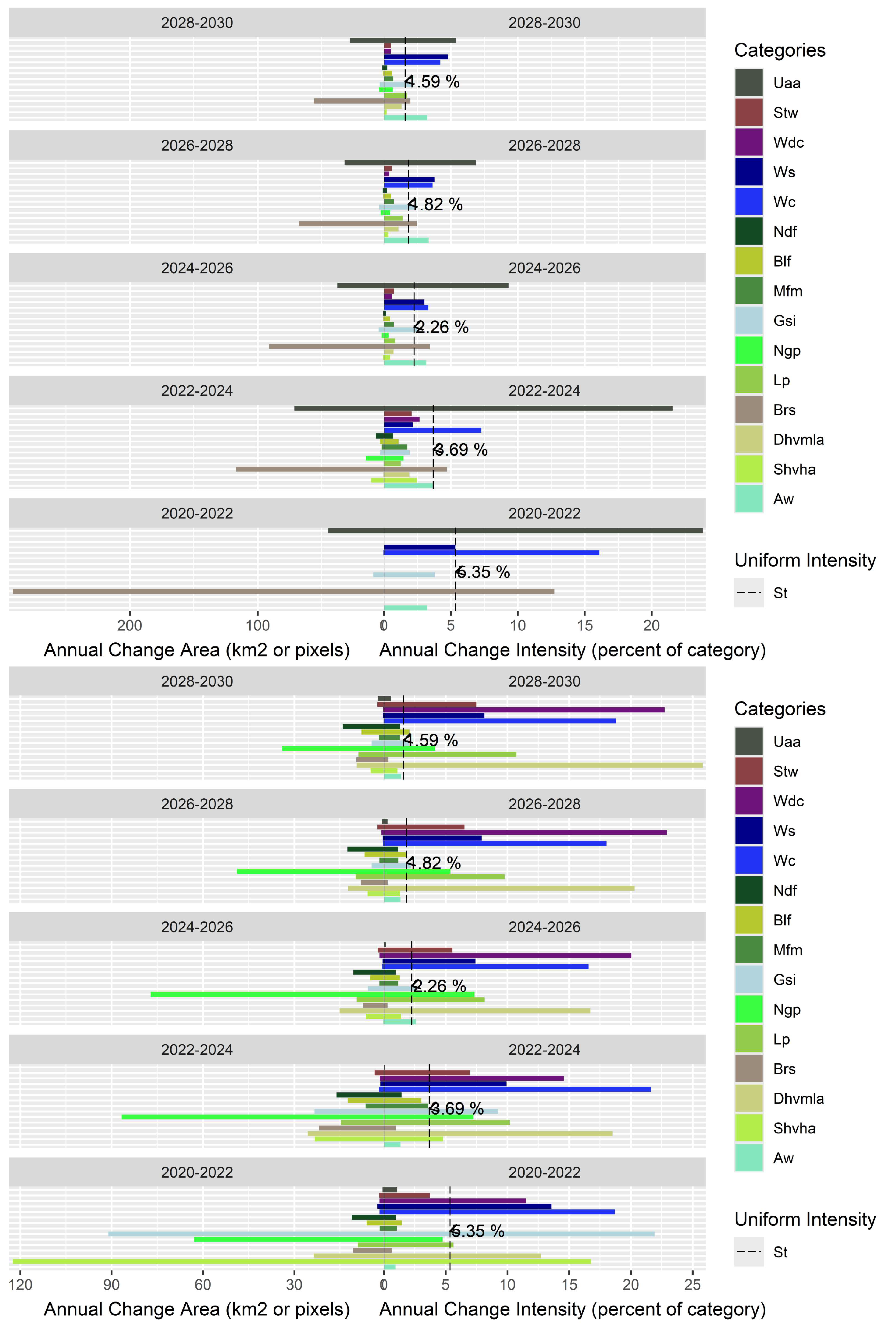
Figure A3.
Transition-level intensity analysis of land cover change for consecutive two-year intervals from 2020 to 2030. Upper panels report the annual area of dominant transitions (km2/year), while lower panels show annual transition intensity (% of the source category’s area per year). Dashed vertical lines indicate the uniform transition intensity (Vtm) for each interval; transitions whose bars exceed this reference level are disproportionately intense. Only the most relevant transitions per interval are shown. Colours follow the reclassified LC legend (Table 1).
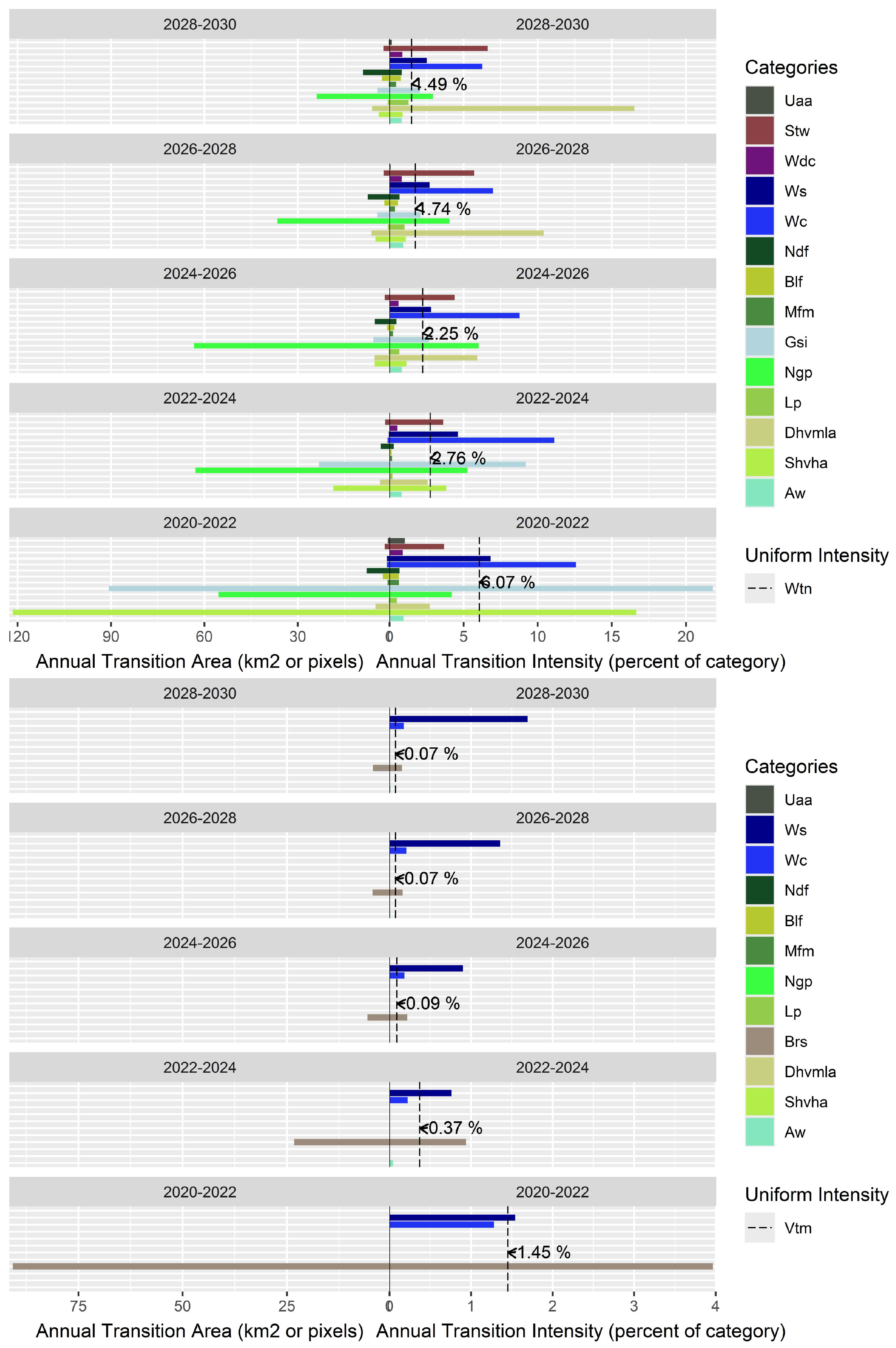
One-step chord diagrams of land cover transitions (2020–2030) (Figure A4)
The chord diagrams visually corroborate these dynamics, with the Ngp-to-Brs transition consistently forming the widest connection across all intervals. Concurrently, the Brs arc progressively expands, while the Ngp and Gsi arcs contract, reflecting their respective net gains and losses. Forest categories display dominant self-loops, confirming strong persistence. Urban areas show thin but consistent inflow ribbons from herbaceous classes, indicating low-intensity yet persistent anthropogenic expansion.
Figure A4.
Sequence of one-step chord diagrams illustrating land cover transitions over consecutive two-year periods (2020–2022, 2022–2024, 2024–2026, 2026–2028, and 2028–2030). The upper panel summarizes overall changes from 2020 to 2030, while the lower panel details transitions for each two-year interval (top: 2020–2022, 2022–2024, and 2024–2026; bottom: 2026–2028, 2028–2030, and 2024–2030). Analyses include the full regional extent, combining observed data (up to 2024) with simulations. Chord widths represent transition areas (km2), and self-loops indicate persistence. Categories follow the circular arrangement and colour scheme of the reclassified legend (Table 1).
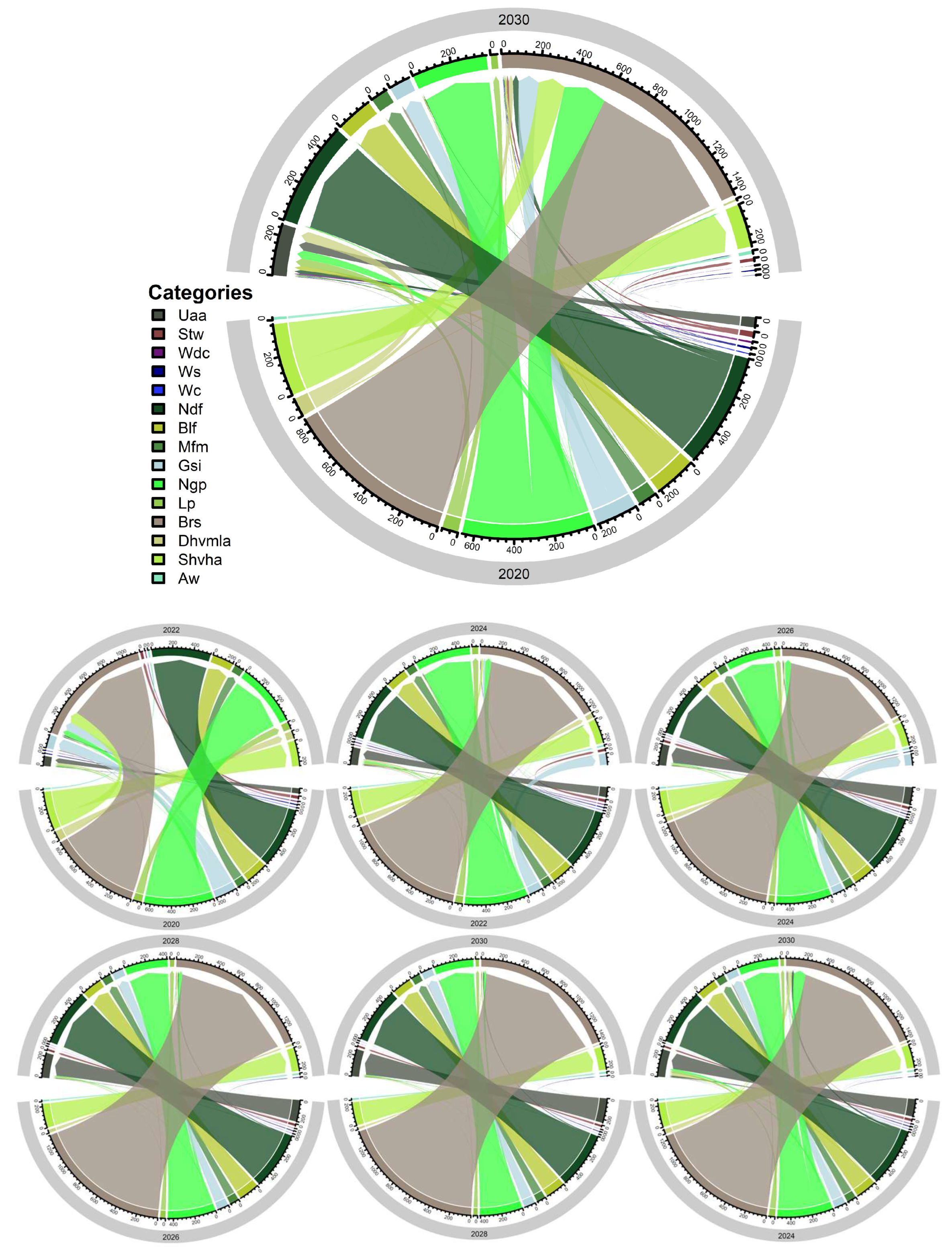
Landscape-level intensity and gross/net change summary (2020–2030) (Figure A5)
At the landscape scale, change intensity is highest during 2020–2022 and subsequently declines across later intervals. Gross–net change decomposition confirms a markedly asymmetric system: Brs acts as the dominant landscape sink with the largest net gain (~+550–600 km2), Ngp represents the largest net loss (~−500 to −600 km2), and Gsi undergoes a substantial decline (~−200 km2). Urban and anthropic areas record a moderate but clear net increase, while forest categories remain broadly stable.
Figure A5.
Interval-level and category-level analysis of land cover change from 2020 to 2030. The upper panel presents interval-level intensity across consecutive two-year periods (2020–2022 to 2028–2030), with bars showing annual change as a percentage of the total mapped area, separated into fast (red) and slow (green) change. The dashed vertical line marks the uniform intensity (U) for each interval; bars exceeding U indicate disproportionately intense change. The lower panel reports gross and net LC changes for each reclassified category over 2020–2030 (km2), with grey bars representing gross change, green bars net gains, and red bars net losses.
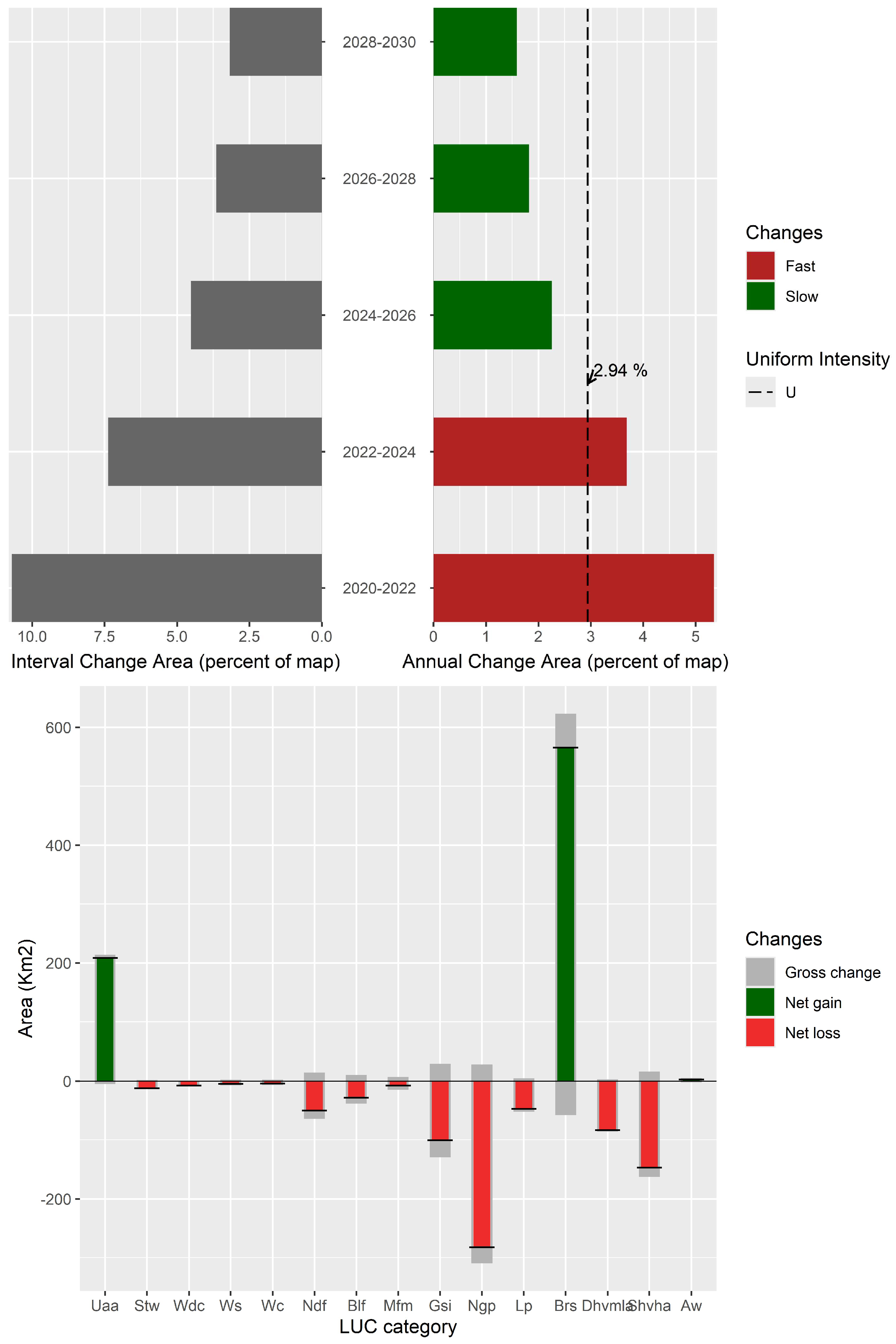
Focused HP and SP maps
Some focused zoomed-in maps with and without population involving HP and SP are provided in the Supplementary Materials.
References
- Amani, M.; Ghorbanian, A.; Ahmadi, S.A.; Kakooei, M.; Moghimi, A.; Mirmazloumi, S.M.; Moghaddam, S.H.A.; Mahdavi, S.; Ghahremanloo, M.; Parsian, S.; et al. Google Earth Engine Cloud Computing Platform for Remote Sensing Big Data Applications: A Comprehensive Review. IEEE J. Sel. Top. Appl. Earth Obs. Remote Sens. 2020, 13, 5326–5350. [Google Scholar] [CrossRef] [Scilit]
- AlAli, R. Artificial Intelligence for Land Cover and Land Use Classification in Remote Sensing: Review Study. Int. Arch. Photogramm. Remote Sens. Spat. Inf. Sci. 2025, 48, 115–122. [Google Scholar] [CrossRef] [Scilit]
- Cheng, X.; Vischer, M.; Schellin, Z.; Arras, L.; Kuglitsch, M.M.; Samek, W.; Ma, J. Explainability in geoAI. In Handbook of Geospatial Artificial Intelligence; CRC Press: Boca Raton, FL, USA, 2023; pp. 177–200. [Google Scholar]
- Agbaje, T.H.; Abomaye-Nimenibo, N.; Ezeh, C.J.; Bello, A.; Olorunnishola, A. Building Damage Assessment in Aftermath of Disaster Events by Leveraging Geoai (Geospatial Artificial Intelligence). World J. Adv. Res. Rev. 2024, 23, 667–687. [Google Scholar] [CrossRef] [Scilit]
- Kang, Y. GeoAI Application Areas and Research Trends. J. Korean Geogr. Soc. 2023, 58, 395–418. [Google Scholar]
- Orusa, T.; Viani, A.; Borgogno-Mondino, E. IRIDE, the Euro-Italian Earth Observation Program: Overview, Current Progress, Global Expectations, and Recommendations. Environ. Sci. Proc. 2024, 29, 74. [Google Scholar]
- Das, S.; Sun, Q.C.; Zhou, H. GeoAI to Implement an Individual Tree Inventory: Framework and Application of Heat Mitigation. Urban For. Urban Green. 2022, 74, 127634. [Google Scholar] [CrossRef] [Scilit]
- Peng, M.; Liu, Y.; Khan, A.; Ahmed, B.; Sarker, S.K.; Ghadi, Y.Y.; Bhatti, U.A.; Al-Razgan, M.; Ali, Y.A. Crop Monitoring Using Remote Sensing Land Use and Land Change Data: Comparative Analysis of Deep Learning Methods Using Pre-Trained CNN Models. Big Data Res. 2024, 36, 100448. [Google Scholar] [CrossRef] [Scilit]
- Carella, E.; Orusa, T.; Viani, A.; Meloni, D.; Borgogno-Mondino, E.; Orusa, R. An Integrated, Tentative Remote-Sensing Approach Based on NDVI Entropy to Model Canine Distemper Virus in Wildlife and to Prompt Science-Based Management Policies. Animals 2022, 12, 1049. [Google Scholar] [CrossRef] [Scilit]
- Helber, P.; Bischke, B.; Dengel, A.; Borth, D. Eurosat: A Novel Dataset and Deep Learning Benchmark for Land Use and Land Cover Classification. IEEE J. Sel. Top. Appl. Earth Obs. Remote Sens. 2019, 12, 2217–2226. [Google Scholar] [CrossRef] [Scilit]
- Viani, A.; Orusa, T.; Borgogno-Mondino, E.; Orusa, R. Snow Metrics as Proxy to Assess Sarcoptic Mange in Wild Boar: Preliminary Results in Aosta Valley (Italy). Life 2023, 13, 987. [Google Scholar] [CrossRef] [Scilit] [PubMed]
- Sefrin, O.; Riese, F.M.; Keller, S. Deep Learning for Land Cover Change Detection. Remote Sens. 2020, 13, 78. [Google Scholar] [CrossRef] [Scilit]
- Wu, Z.; Ma, P.; Zheng, Y.; Gu, F.; Liu, L.; Lin, H. Automatic Detection and Classification of Land Subsidence in Deltaic Metropolitan Areas Using Distributed Scatterer InSAR and Oriented R-CNN. Remote Sens. Environ. 2023, 290, 113545. [Google Scholar] [CrossRef] [Scilit]
- Yang, L.; Driscol, J.; Sarigai, S.; Wu, Q.; Chen, H.; Lippitt, C.D. Google Earth Engine and Artificial Intelligence (AI): A Comprehensive Review. Remote Sens. 2022, 14, 3253. [Google Scholar]
- Yang, Y.; Erskine, P.D.; Lechner, A.M.; Mulligan, D.; Zhang, S.; Wang, Z. Detecting the Dynamics of Vegetation Disturbance and Recovery in Surface Mining Area via Landsat Imagery and LandTrendr Algorithm. J. Clean. Prod. 2018, 178, 353–362. [Google Scholar] [CrossRef] [Scilit]
- Yang, C.; Rottensteiner, F.; Heipke, C. Classification of Land Cover and Land Use Based on Convolutional Neural Networks. ISPRS Ann. Photogramm. Remote Sens. Spat. Inf. Sci. 2018, 4, 251–258. [Google Scholar] [CrossRef] [Scilit]
- Yan, C.; Fan, X.; Fan, J.; Yu, L.; Wang, N.; Chen, L.; Li, X. Hyformer: Hybrid Transformer and Cnn for Pixel-Level Multispectral Image Land Cover Classification. Int. J. Environ. Res. Public Health 2023, 20, 3059. [Google Scholar] [CrossRef] [Scilit]
- Arundel, S.T.; McKeehan, K.G.; Li, W.; Gu, Z. GeoAI for Spatial Image Processing. In Handbook of Geospatial Artificial Intelligence; CRC Press: Boca Raton, FL, USA, 2023; pp. 75–98. [Google Scholar]
- Boutayeb, A.; Lahsen-cherif, I.; Khadimi, A.E. A Comprehensive GeoAI Review: Progress, Challenges and Outlooks. arXiv 2024, arXiv:2412.11643. [Google Scholar] [CrossRef] [Scilit]
- Boutayeb, A.; Lahsen-Cherif, I.; El Khadimi, A. When Machine Learning Meets Geospatial Data: A Comprehensive GeoAI Review. IEEE J. Sel. Top. Appl. Earth Obs. Remote Sens. 2025, 18, 13135–13191. [Google Scholar]
- Chen, D. Exemplification on Potential Applications and Scenarios for geoAI. In 2023 Asia-Europe Conference on Electronics, Data Processing and Informatics (ACEDPI); IEEE: New York, NY, USA, 2023; pp. 245–248. [Google Scholar]
- Orusa, T.; Viani, A.; Borgogno-Mondino, E. Earth Observation Data and Geospatial Deep Learning AI to Assign Contributions to European Municipalities Sen4MUN: An Empirical Application in Aosta Valley (NW Italy). Land 2024, 13, 80. [Google Scholar] [CrossRef] [Scilit]
- Alesheikh, A.A.; Helali, H.; Behroz, H. Web GIS: Technologies and Its Applications. In Symposium on Geospatial Theory, Processing and Applications; ISPRS: Hannover, Germany, 2002; Volume 15, pp. 1–9. [Google Scholar]
- Adnan, M.; Singleton, A.; Longley, P. Developing Efficient Web-Based GIS Applications; Centre for Advanced Spatial Analysis (UCL): London, UK, 2010. [Google Scholar]
- Chipatiso, E. Application of GIS and Artificial Intelligence in Military Operations: Prospects and Challenges. S. Afr. J. Secur. 2025, 3, 15984. [Google Scholar] [CrossRef] [Scilit] [PubMed]
- Parracciani, C.; Gigante, D.; Mutanga, O.; Bonafoni, S.; Vizzari, M. Land Cover Changes in Grassland Landscapes: Combining Enhanced Landsat Data Composition, LandTrendr, and Machine Learning Classification in Google Earth Engine with MLP-ANN Scenario Forecasting. GIScience Remote Sens. 2024, 61, 2302221. [Google Scholar] [CrossRef] [Scilit]
- Orusa, T.; Orusa, R.; Viani, A.; Carella, E.; Borgogno Mondino, E. Geomatics and EO Data to Support Wildlife Diseases Assessment at Landscape Level: A Pilot Experience to Map Infectious Keratoconjunctivitis in Chamois and Phenological Trends in Aosta Valley (NW Italy). Remote Sens. 2020, 12, 3542. [Google Scholar] [CrossRef] [Scilit]
- Aldwaik, S.Z.; Pontius, R.G., Jr. Intensity Analysis to Unify Measurements of Size and Stationarity of Land Changes by Interval, Category, and Transition. Landsc. Urban Plan. 2012, 106, 103–114. [Google Scholar] [CrossRef] [Scilit]
- Goicolea, T.; Cisneros-Araújo, P.; Vega, C.A.; Sánchez-Vizcaíno, J.M.; Mateo-Sánchez, M.; Bosch, J. Landscape Connectivity for Predicting the Spread of ASF in the European Wild Boar Population. Sci. Rep. 2024, 14, 3414. [Google Scholar] [CrossRef] [Scilit]
- Amponsah, A.; Latue, P.; Rakuasa, H. Utilization of GeoAI Applications in the Health Sector: A Review. J. Health Sci. Med. Ther. 2023, 1, 49–60. [Google Scholar] [CrossRef] [Scilit]
- De Sabbata, S.; Ballatore, A.; Miller, H.J.; Sieber, R.; Tyukin, I.; Yeboah, G. GeoAI in Urban Analytics. Int. J. Geogr. Inf. Sci. 2023, 37, 2455–2463. [Google Scholar] [CrossRef] [Scilit]
- Kamel Boulos, M.N.; Peng, G.; VoPham, T. An Overview of GeoAI Applications in Health and Healthcare. Int. J. Health Geogr. 2019, 18, 7. [Google Scholar] [CrossRef] [Scilit]
- Gonzales-Inca, C.; Calle, M.; Croghan, D.; Torabi Haghighi, A.; Marttila, H.; Silander, J.; Alho, P. Geospatial Artificial Intelligence (GeoAI) in the Integrated Hydrological and Fluvial Systems Modeling: Review of Current Applications and Trends. Water 2022, 14, 2211. [Google Scholar] [CrossRef] [Scilit]
- Orusa, T.; Cammareri, D.; Freppaz, D.; Vuillermoz, P.; Borgogno Mondino, E. Sen4MUN: A Prototypal Service for the Distribution of Contributions to the European Municipalities from Copernicus Satellite Imagery. A Case in Aosta Valley (NW Italy). In Italian Conference on Geomatics and Geospatial Technologies; Springer: Cham, Switzerland, 2023; pp. 109–125. [Google Scholar]
- Mugiraneza, T.; Nascetti, A.; Ban, Y. Continuous Monitoring of Urban Land Cover Change Trajectories with Landsat Time Series and Landtrendr-Google Earth Engine Cloud Computing. Remote Sens. 2020, 12, 2883. [Google Scholar] [CrossRef] [Scilit]
- Viani, A.; Orusa, T.; Mandola, M.L.; Robetto, S.; Nogarol, C.; Mondino, E.B.; Orusa, R. Grading Habitats for Ticks by Mapping a Suitability Index Based on Remotely Sensed Data and Meta® Population Dataset in Aosta Valley, NW Italy. Vet. Ital. 2024, 60. [Google Scholar] [CrossRef] [Scilit]
- Viani, A.; Orusa, T.; Divari, S.; Lovisolo, S.; Zanet, S.; Orusa, R.; Borgogno-Mondino, E.; Bollo, E. Detection of Bartonella Spp. in Foxes’ Populations in Piedmont and Aosta Valley (NW Italy) Coupling Geospatially-Based Techniques. Front. Vet. Sci. 2025, 11, 1388440. [Google Scholar] [CrossRef] [Scilit]
- Atef, I.; Ahmed, W.; Abdel-Maguid, R.H. Future Land Use Land Cover Changes in El-Fayoum Governorate: A Simulation Study Using Satellite Data and CA-Markov Model. Stoch. Environ. Res. Risk Assess. 2024, 38, 651–664. [Google Scholar] [CrossRef] [Scilit]
- Aruna Sri, P.; Santhi, V. Enhanced Land Use and Land Cover Classification Using Modified CNN in Uppal Earth Region. Multimed. Tools Appl. 2025, 84, 14941–14964. [Google Scholar] [CrossRef] [Scilit]
- Aryan, A.; Prakash, R.; Aluvala, S.; Chowdary, V.S. Precision Land Use and Land Cover Mapping with a High-Accuracy Time Series LSTM Model. In 2025 IEEE International Students’ Conference on Electrical, Electronics and Computer Science (SCEECS); IEEE: New York, NY, USA, 2025; pp. 1–5. [Google Scholar]
- Gu, Z.; Zeng, M. The Use of Artificial Intelligence and Satellite Remote Sensing in Land Cover Change Detection: Review and Perspectives. Sustainability 2024, 16, 274. [Google Scholar] [CrossRef] [Scilit]
- Livadiotis, E.; Troudi, N.; Gharbia, N.B.; Tzoraki, O. Evaluating the Land Use/Land Cover Change with a Future Prediction Using Remote Sensing and GIS in the Elassona-Tsaritsani Basin of Thessaly (Central Greece). In Euro-Mediterranean Conference for Environmental Integration; Springer: Cham, Switzerland, 2022; pp. 709–713. [Google Scholar]
- Viani, A.; Orusa, T.; Borgogno-Mondino, E.; Orusa, R. A One Health Google Earth Engine Web-GIS Application to Evaluate and Monitor Water Quality Worldwide. Euro-Mediterr. J. Environ. Integr. 2024, 9, 1873–1886. [Google Scholar] [CrossRef] [Scilit]
- De Petris, S.; Orusa, T.; Viani, A.; Feliziani, F.; Sordilli, M.; Troisi, S.; Zoppi, S.; Ragionieri, M.; Orusa, R.; Borgogno-Mondino, E. Spatio-Temporal Pattern Analysis of African Swine Fever Spreading in Northwestern Italy—The Role of Habitat Interfaces. Animals 2025, 15, 2886. [Google Scholar] [CrossRef] [Scilit]
- Tejasree, G.; Agilandeeswari, L. Land Use/Land Cover (LULC) Classification Using Deep-LSTM for Hyperspectral Images. Egypt. J. Remote Sens. Space Sci. 2024, 27, 52–68. [Google Scholar] [CrossRef] [Scilit]
- Orusa, T.; Viani, A.; d’Alessio, S.G.; Orusa, R.; Caminade, C. One Health Approaches and Modeling in Parasitology in the Climate Change Framework and Possible Supporting Tools Adopting GIS and Remote Sensing. Front. Parasitol. 2025, 4, 1560799. [Google Scholar] [CrossRef] [Scilit] [PubMed]
- Li, Z.; Ning, H.; Gao, S.; Janowicz, K.; Li, W.; Arundel, S.T.; Yang, C.; Bhaduri, B.; Wang, S.; Zhu, A.-X.; et al. Giscience in the Era of Artificial Intelligence: A Research Agenda towards Autonomous Gis. Ann. GIS 2025, 31, 501–536. [Google Scholar] [CrossRef] [Scilit]
- Liu, D.; Cai, S. A Spatial-Temporal Modeling Approach to Reconstructing Land-Cover Change Trajectories from Multi-Temporal Satellite Imagery. Ann. Assoc. Am. Geogr. 2012, 102, 1329–1347. [Google Scholar] [CrossRef] [Scilit]
- Lu, T.; Wan, L.; Qi, S.; Gao, M. Land Cover Classification of UAV Remote Sensing Based on Transformer–CNN Hybrid Architecture. Sensors 2023, 23, 5288. [Google Scholar] [CrossRef] [Scilit]
- QGIS Development Team. QGIS Geographic Information System. Open Source Geospatial Foundation Project 2018. Available online: https://qgis.org/resources/support/faq/#how-to-cite-qgis (accessed on 22 March 2026).
- Conrad, O.; Bechtel, B.; Bock, M.; Dietrich, H.; Fischer, E.; Gerlitz, L.; Wehberg, J.; Wichmann, V.; Böhner, J. System for Automated Geoscientific Analyses (SAGA) v. 2.1.4. Geosci. Model Dev. 2015, 8, 1991–2007. [Google Scholar] [CrossRef] [Scilit]
- Aybar, C.; Wu, Q.; Bautista, L.; Yali, R.; Barja, A. Rgee: An R Package for Interacting with Google Earth Engine. J. Open Source Softw. 2020, 5, 2272. [Google Scholar] [CrossRef] [Scilit]
- Wu, Q. Geemap: A Python Package for Interactive Mapping with Google Earth Engine. J. Open Source Softw. 2020, 5, 2305. [Google Scholar] [CrossRef] [Scilit]
- Gorelick, N.; Hancher, M.; Dixon, M.; Ilyushchenko, S.; Thau, D.; Moore, R. Google Earth Engine: Planetary-Scale Geospatial Analysis for Everyone. Remote Sens. Environ. 2017, 202, 18–27. [Google Scholar] [CrossRef] [Scilit]
- Gorelick, N. Google Earth Engine. In EGU General Assembly Conference Abstracts; American Geophysical Union: Vienna, Austria, 2013; Volume 15, p. 11997. [Google Scholar]
- Alshari, E.A.; Gawali, B.W. Modeling Land Use Change in Sana’a City of Yemen with MOLUSCE. J. Sens. 2022, 2022, 7419031. [Google Scholar] [CrossRef] [Scilit]
- Baghel, S.; Kothari, M.; Tripathi, M.; Singh, P.K.; Bhakar, S.R.; Dave, V.; Jain, S. Spatiotemporal LULC Change Detection and Future Prediction for the Mand Catchment Using MOLUSCE Tool. Environ. Earth Sci. 2024, 83, 66. [Google Scholar] [CrossRef] [Scilit]
- Gündüz, H.İ. Land-Use Land-Cover Dynamics and Future Projections Using GEE, ML, and QGIS-MOLUSCE: A Case Study in Manisa. Sustainability 2025, 17, 1363. [Google Scholar] [CrossRef] [Scilit]
- Amgoth, A.; Rani, H.P.; Jayakumar, K. Exploring LULC Changes in Pakhal Lake Area, Telangana, India Using QGIS MOLUSCE Plugin. Spat. Inf. Res. 2023, 31, 429–438. [Google Scholar] [CrossRef] [Scilit]
- Bathe, K.D.; Patil, N.S. Assessment of Land Use-Land Cover Dynamics and Its Future Projection through Google Earth Engine, Machine Learning and QGIS-MOLUSCE: A Case Study in Jagatsinghpur District, Odisha, India. J. Earth Syst. Sci. 2024, 133, 111. [Google Scholar] [CrossRef] [Scilit]
- Kamaraj, M.; Rangarajan, S. Predicting the Future Land Use and Land Cover Changes for Bhavani Basin, Tamil Nadu, India, Using QGIS MOLUSCE Plugin. Environ. Sci. Pollut. Res. 2022, 29, 86337–86348. [Google Scholar] [CrossRef] [Scilit] [PubMed]
- Orusa, T.; Viani, A.; Cammareri, D.; Borgogno Mondino, E. A Google Earth Engine Algorithm to Map Phenological Metrics in Mountain Areas Worldwide with Landsat Collection and Sentinel-2. Geomatics 2023, 3, 221–238. [Google Scholar] [CrossRef] [Scilit]
- Muhammad, R.; Zhang, W.; Abbas, Z.; Guo, F.; Gwiazdzinski, L. Spatiotemporal Change Analysis and Prediction of Future Land Use and Land Cover Changes Using QGIS MOLUSCE Plugin and Remote Sensing Big Data: A Case Study of Linyi, China. Land 2022, 11, 419. [Google Scholar] [CrossRef] [Scilit]
- Roy, S.K.; Kumar, A. Monitoring the LULC Changes in the Rurban Region of Berhampore Municipality Using MOLUSCE Plugin of QGIS. Proc. Indian Natl. Sci. Acad. 2025. [Google Scholar] [CrossRef] [Scilit]
- Rudewicz, J. Theoretical Insights into Artificial Intelligence Applications in Human Geography and Spatial Management (GeoAI). Eur. Res. Stud. J. 2024, 27, 973–984. [Google Scholar] [CrossRef] [Scilit]
- Xing, J.; Sieber, R. Integrating XAI and GeoAI. 2021. Available online: https://escholarship.org/uc/item/9vv6j0m9 (accessed on 22 March 2026).
- Wu, M.; Huang, Q.; Gao, S. Advancing Vision-Language Models with Spatial-Context Prompt Tuning: A Case Study in GeoAI-Empowered Image Geo-Localization. J. Locat. Based Serv. 2025, 1–21. [Google Scholar] [CrossRef] [Scilit]
- VoPham, T.; Hart, J.E.; Laden, F.; Chiang, Y.-Y. Emerging Trends in Geospatial Artificial Intelligence (geoAI): Potential Applications for Environmental Epidemiology. Environ. Health 2018, 17, 40. [Google Scholar] [CrossRef] [Scilit]
- Viani, A.; Orusa, T.; Divari, S.; Lovisolo, S.; Zanet, S.; Borgogno-Mondino, E.; Orusa, R.; Bollo, E. Bartonella Spp. Distribution Assessment in Foxes Coupling Geospatially-Based Techniques. In Earth Observation: Current Challenges and Opportunities for Environmental Monitoring; Associazione Italiana di Telerilevamento (AIT): Firenze, Italy, 2024; Volume 3, pp. 50–55. [Google Scholar]
- Akinboyewa, T.; Li, Z.; Ning, H.; Lessani, M.N. GIS Copilot: Towards an Autonomous GIS Agent for Spatial Analysis. Int. J. Digit. Earth 2025, 18, 2497489. [Google Scholar] [CrossRef] [Scilit]
- Arrechea-Castillo, D.A.; Solano-Correa, Y.T.; Muñoz-Ordóñez, J.F.; Pencue-Fierro, E.L.; Figueroa-Casas, A. Multiclass Land Use and Land Cover Classification of Andean Sub-Basins in Colombia with Sentinel-2 and Deep Learning. Remote Sens. 2023, 15, 2521. [Google Scholar] [CrossRef] [Scilit]
- Basu, T.; Das, A.; Pham, Q.B.; Al-Ansari, N.; Linh, N.T.T.; Lagerwall, G. Development of an Integrated Peri-Urban Wetland Degradation Assessment Approach for the Chatra Wetland in Eastern India. Sci. Rep. 2021, 11, 4470. [Google Scholar] [PubMed]
- Bianchi, O.; Putro, H.P. Artificial Intelligence in Environmental Monitoring: Predicting and Managing Climate Change Impacts. Int. Trans. Artif. Intell. 2024, 3, 85–96. [Google Scholar] [CrossRef] [Scilit]
- Blissag, B.; Yebdri, D.; Kessar, C. Spatiotemporal Change Analysis of LULC Using Remote Sensing and CA-ANN Approach in the Hodna Basin, NE of Algeria. Phys. Chem. Earth Parts A/B/C 2024, 133, 103535. [Google Scholar] [CrossRef] [Scilit]
- Bozali, N. Spatiotemporal Simulation of Land Use and Land Cover Changes in Türkiye through a CA–Markov Framework. Sci. Rep. 2026, 16, 5320. [Google Scholar] [CrossRef] [Scilit]
- Bui, Q.-T.; Chou, T.-Y.; Hoang, T.-V.; Fang, Y.-M.; Mu, C.-Y.; Huang, P.-H.; Pham, V.-D.; Nguyen, Q.-H.; Anh, D.T.N.; Pham, V.-M.; et al. Gradient Boosting Machine and Object-Based CNN for Land Cover Classification. Remote Sens. 2021, 13, 2709. [Google Scholar] [CrossRef] [Scilit]
- Orusa, T.; Mondino, E.B. Landsat 8 Thermal Data to Support Urban Management and Planning in the Climate Change Era: A Case Study in Torino Area, NW Italy. In Remote Sensing Technologies and Applications in Urban Environments IV; International Society for Optics and Photonics: Bellingham, WA, USA, 2019; Volume 11157, p. 111570O. [Google Scholar]
- Orusa, T.; Viani, A.; Di Lorenzo, A.; Orusa, R. CerMapp: A Cloud-Based Geospatial Prototype for National Wildlife Disease Surveillance. ISPRS Int. J. Geo-Inf. 2025, 14, 453. [Google Scholar] [CrossRef] [Scilit]
- Geng, Q.; Wang, L.; Li, Q. Soil Temperature Prediction Based on Explainable Artificial Intelligence and LSTM. Front. Environ. Sci. 2024, 12, 1426942. [Google Scholar] [CrossRef] [Scilit]
- Viani, A.; Orusa, T.; Mandola, M.L.; Robetto, S.; Belvedere, M.; Renna, G.; Scala, S.; Borgogno-Mondino, E.; Orusa, R. R05. 4 Tick’s Suitability Habitat Maps and Tick-Host Relationships in Wildlife. A One Health Approach Based on Multitemporal Remote Sensed Data, Entropy and Meta® Population Dataset in Aosta Valley, NW Italy. In Proceedings of the GeoVet 2023 International Conference, Silvi Marina, Italy, 19–21 September 2023. [Google Scholar]
- Mohanrajan, S.N.; Loganathan, A. Novel Vision Transformer–Based Bi-LSTM Model for LU/LC Prediction—Javadi Hills, India. Appl. Sci. 2022, 12, 6387. [Google Scholar] [CrossRef] [Scilit]
- Rajendran, G.B.; Kumarasamy, U.M.; Zarro, C.; Divakarachari, P.B.; Ullo, S.L. Land-Use and Land-Cover Classification Using a Human Group-Based Particle Swarm Optimization Algorithm with an LSTM Classifier on Hybrid Pre-Processing Remote-Sensing Images. Remote Sens. 2020, 12, 4135. [Google Scholar] [CrossRef] [Scilit]
- Varma, B.; Naik, N.; Chandrasekaran, K.; Venkatesan, M.; Rajan, J. Forecasting Land-Use and Land-Cover Change Using Hybrid Cnn–Lstm Model. IEEE Geosci. Remote Sens. Lett. 2024, 21, 8001805. [Google Scholar] [CrossRef] [Scilit]
- Wang, H.; Zhao, X.; Zhang, X.; Wu, D.; Du, X. Long Time Series Land Cover Classification in China from 1982 to 2015 Based on Bi-LSTM Deep Learning. Remote Sens. 2019, 11, 1639. [Google Scholar] [CrossRef] [Scilit]
- Orusa, T.; Borgogno Mondino, E. Exploring Short-Term Climate Change Effects on Rangelands and Broad-Leaved Forests by Free Satellite Data in Aosta Valley (Northwest Italy). Climate 2021, 9, 47. [Google Scholar] [CrossRef] [Scilit]
- Orusa, T.; Farbo, A.; De Petris, S.; Sarvia, F.; Cammareri, D.; Borgogno-Mondino, E. Characterization of Alpine Pastures Using Multitemporal Earth Observation Data within the Climate Change Framework. In Earth Observation: Current Challenges and Opportunities for Environmental Monitoring; Associazione Italiana di Telerilevamento (AIT): Firenze, Italy, 2024; Volume 3, pp. 110–114. [Google Scholar]
- Censi, A.M.; Ienco, D.; Gbodjo, Y.J.E.; Pensa, R.G.; Interdonato, R.; Gaetano, R. Attentive Spatial Temporal Graph CNN for Land Cover Mapping from Multi Temporal Remote Sensing Data. IEEE Access 2021, 9, 23070–23082. [Google Scholar] [CrossRef] [Scilit]
- Chambers, J.M. Extending R; Chapman and Hall/CRC: Boca Raton, FL, USA, 2017. [Google Scholar]
- Orusa, T.; Viani, A.; Moyo, B.; Cammareri, D.; Borgogno-Mondino, E. Risk Assessment of Rising Temperatures Using Landsat 4–9 LST Time Series and Meta® Population Dataset: An Application in Aosta Valley, NW Italy. Remote Sens. 2023, 15, 2348. [Google Scholar] [CrossRef] [Scilit]
- Chamling, M.; Bera, B.; Sarkar, S. Geospatial Environmental Modeling of Forest Declining Trend in Eastern Himalayan Biodiversity Hotspot Region. In Forest Resources Resilience and Conflicts; Elsevier: Amsterdam, The Netherlands, 2021; pp. 417–433. [Google Scholar]
- Chen, Y. Monitoring Land Use/Land Cover Change (LULCC) Using Remote Sensing. In E3S Web of Conferences; EDP Sciences: Les Ulis, France, 2023; Volume 424, p. 03002. [Google Scholar]
- Dalgaard, P. Introductory Statistics with R; Springer: New York, NY, USA, 2002. [Google Scholar]
- Das, B.; Prasad, J. Cellular Automata (CA) and AI-Based Recurrent Neural Networks (RNNs) Approaches in Land Use Land Cover (LULC) Change Dynamics Using Multi-Spectral and Multi-Decadal Landsat Data in Haldia, India. Remote Sens. Earth Syst. Sci. 2025, 8, 1223–1243. [Google Scholar] [CrossRef] [Scilit]
- Orusa, T.; Cammareri, D.; Borgogno Mondino, E. A Scalable Earth Observation Service to Map Land Cover in Geomorphological Complex Areas beyond the Dynamic World: An Application in Aosta Valley (NW Italy). Appl. Sci. 2022, 13, 390. [Google Scholar] [CrossRef] [Scilit]
- Orusa, T.; Cammareri, D.; Borgogno Mondino, E. A Possible Land Cover EAGLE Approach to Overcome Remote Sensing Limitations in the Alps Based on Sentinel-1 and Sentinel-2: The Case of Aosta Valley (NW Italy). Remote Sens. 2022, 15, 178. [Google Scholar] [CrossRef] [Scilit]
- Field, A.; Field, Z.; Miles, J. Discovering Statistics Using R; SAGE Publications Ltd.: Thousand Oaks, CA, USA, 2012. [Google Scholar]
- Qian, S.S. Environmental and Ecological Statistics with R; Chapman and Hall/CRC: Boca Raton, FL, USA, 2016. [Google Scholar]
- Reimann, C.; Filzmoser, P.; Garrett, R.; Dutter, R. Statistical Data Analysis Explained: Applied Environmental Statistics with R; John Wiley & Sons: Hoboken, NJ, USA, 2011. [Google Scholar]
- Ugarte, M.D.; Militino, A.F.; Arnholt, A.T. Probability and Statistics with R; CRC Press: Boca Raton, FL, USA, 2008. [Google Scholar]
- Webster, R.; Oliver, M.A. Geostatistics for Environmental Scientists; John Wiley & Sons: Hoboken, NJ, USA, 2007. [Google Scholar]
- Wikle, C.K.; Zammit-Mangion, A.; Cressie, N. Spatio-Temporal Statistics with R; Chapman and Hall/CRC: Boca Raton, FL, USA, 2019. [Google Scholar]
- Dewangkoro, H.; Arymurthy, A.M. Land Use and Land Cover Classification Using CNN, SVM, and Channel Squeeze & Spatial Excitation Block. In IOP Conference Series: Earth and Environmental Science; IOP Publishing: Bristol, UK, 2021; Volume 704, p. 012048. [Google Scholar]
- Eastman, J.; Toledano, J. A Short Presentation of CA_MARKOV. In Geomatic Approaches for Modeling Land Change Scenarios; Springer: Cham, Switzerland, 2017; pp. 481–484. [Google Scholar]
- Ergen, M. Spatıotemporal Analysıs of Urban Development and Land USE in Sakarya Provınce, Türkiye: Implıcatıons for Future Urban Growth Modelıng. GeoJournal 2025, 90, 112. [Google Scholar] [CrossRef] [Scilit]
- Fan, R.; Feng, R.; Wang, L.; Yan, J.; Zhang, X. Semi-MCNN: A Semisupervised Multi-CNN Ensemble Learning Method for Urban Land Cover Classification Using Submeter HRRS Images. IEEE J. Sel. Top. Appl. Earth Obs. Remote Sens. 2020, 13, 4973–4987. [Google Scholar] [CrossRef] [Scilit]
- Gaetano, R.; Ienco, D.; Ose, K.; Cresson, R. A Two-Branch CNN Architecture for Land Cover Classification of PAN and MS Imagery. Remote Sens. 2018, 10, 1746. [Google Scholar] [CrossRef] [Scilit]
- Gao, C.; Cheng, D.; Iqbal, J.; Yao, S. Spatiotemporal Change Analysis and Prediction of the Great Yellow River Region (GYRR) Land Cover and the Relationship Analysis with Mountain Hazards. Land 2023, 12, 340. [Google Scholar] [CrossRef] [Scilit]
- Gao, S.; Hu, Y.; Li, W. Introduction to Geospatial Artificial Intelligence (GeoAI). In Handbook of Geospatial Artificial Intelligence; CRC Press: Boca Raton, FL, USA, 2023; pp. 3–16. [Google Scholar]
- Exavier, R.; Zeilhofer, P. OpenLand: Software for Quantitative Analysis and Visualization of Land Use and Cover Change. R J. 2020, 12, 373–388. [Google Scholar] [CrossRef] [Scilit]
- Gu, Z.; Gu, L.; Eils, R.; Schlesner, M.; Brors, B. “Circlize” Implements and Enhances Circular Visualization in R. Bioinformatics 2014, 30, 2811–2812. [Google Scholar] [CrossRef] [Scilit]
- Hasan, I.; Goni, O.; Katha, Z.T.; Rabby, M.I.; Hossain, S.; Banik, A.; Hasan, S.; Rahman, I. Prediction Modeling of Land Surface Temperature in Relation to Land Cover Dynamics and Health Risk Perception Analysis in Barishal City of Bangladesh. Sci. Rep. 2025, 15, 30730. [Google Scholar] [CrossRef] [Scilit] [PubMed]
- Ienco, D.; Gbodjo, Y.J.E.; Gaetano, R.; Interdonato, R. Weakly Supervised Learning for Land Cover Mapping of Satellite Image Time Series via Attention-Based CNN. IEEE Access 2020, 8, 179547–179560. [Google Scholar] [CrossRef] [Scilit]
- Ji, R.; Tan, K.; Wang, X.; Tang, S.; Sun, J.; Niu, C.; Pan, C. PatchOut: A Novel Patch-Free Approach Based on a Transformer-CNN Hybrid Framework for Fine-Grained Land-Cover Classification on Large-Scale Airborne Hyperspectral Images. Int. J. Appl. Earth Obs. Geoinf. 2025, 138, 104457. [Google Scholar] [CrossRef] [Scilit]
- Kang, Y.; Gao, S.; Roth, R. A Review and Synthesis of Recent Geoai Research for Cartography: Methods, Applications, and Ethics. In Proceedings of the AutoCarto, Redlands, CA, USA, 2–4 November 2022; pp. 2–4. [Google Scholar]
- Kang, Y.; Gao, S.; Roth, R.E. Artificial Intelligence Studies in Cartography: A Review and Synthesis of Methods, Applications, and Ethics. Cartogr. Geogr. Inf. Sci. 2024, 51, 599–630. [Google Scholar] [CrossRef] [Scilit]
- Kaur, A.; Singh, G.; Singh, S. AI-Driven Tools and Technologies for Agriculture Land Use & Land Cover Classification Using Earth Observation Data Analytics. In Google Earth Engine and Artificial Intelligence for Earth Observation; Elsevier: Amsterdam, The Netherlands, 2025; pp. 527–541. [Google Scholar]
- Liu, P.; Biljecki, F. A Review of Spatially-Explicit GeoAI Applications in Urban Geography. Int. J. Appl. Earth Obs. Geoinf. 2022, 112, 102936. [Google Scholar] [CrossRef] [Scilit]
- Lu, F.; Cheng, S.; Wang, P. GeoAI Enabled Urban Computing: Status and Challenges. Ann. GIS 2025, 31, 537–555. [Google Scholar] [CrossRef] [Scilit]
- Mai, G.; Janowicz, K.; Hu, Y.; Gao, S.; Yan, B.; Zhu, R.; Cai, L.; Lao, N. A Review of Location Encoding for GeoAI: Methods and Applications. Int. J. Geogr. Inf. Sci. 2022, 36, 639–673. [Google Scholar] [CrossRef] [Scilit]
- Memon, N.; Parikh, H.; Patel, S.B.; Patel, D.; Patel, V.D. Automatic Land Cover Classification of Multi-Resolution Dualpol Data Using Convolutional Neural Network (CNN). Remote Sens. Appl. Soc. Environ. 2021, 22, 100491. [Google Scholar] [CrossRef] [Scilit]
- Moore, R.; Hansen, M. Google Earth Engine: A New Cloud-Computing Platform for Global-Scale Earth Observation Data and Analysis. In Proceedings of the AGU Fall Meeting Abstracts, San Francisco, CA, USA, 5–9 December 2011; Volume 2011, p. IN43C-02. [Google Scholar]
- Muenchow, J.; Schratz, P.; Brenning, A. RQGIS: Integrating R with QGIS for Statistical Geocomputing. R J. 2017, 9, 409–428. [Google Scholar] [CrossRef] [Scilit]
- Allen, T.R.; Wong, D.W. Exploring GIS, Spatial Statistics and Remote Sensing for Risk Assessment of Vector-Borne Diseases: A West Nile Virus Example. Int. J. Risk Assess. Manag. 2006, 6, 253–275. [Google Scholar] [CrossRef] [Scilit]
- Osco, L.P.; Wu, Q.; De Lemos, E.L.; Gonçalves, W.N.; Ramos, A.P.M.; Li, J.; Junior, J.M. The Segment Anything Model (Sam) for Remote Sensing Applications: From Zero to One Shot. Int. J. Appl. Earth Obs. Geoinf. 2023, 124, 103540. [Google Scholar] [CrossRef] [Scilit]
- Pan, S.; Guan, H.; Chen, Y.; Yu, Y.; Gonçalves, W.N.; Junior, J.M.; Li, J. Land-Cover Classification of Multispectral LiDAR Data Using CNN with Optimized Hyper-Parameters. ISPRS J. Photogramm. Remote Sens. 2020, 166, 241–254. [Google Scholar] [CrossRef] [Scilit]
- Pierdicca, R.; Paolanti, M. GeoAI: A Review of Artificial Intelligence Approaches for the Interpretation of Complex Geomatics Data. Geosci. Instrum. Methods Data Syst. Discuss. 2022, 11, 195–218. [Google Scholar] [CrossRef] [Scilit]
- Ramanath, A.; Muthusrinivasan, S.; Xie, Y.; Shekhar, S.; Ramachandra, B. Ndvi versus Cnn Features in Deep Learning for Land Cover Clasification of Aerial Images. In IGARSS 2019—2019 IEEE International Geoscience and Remote Sensing Symposium; IEEE: New York, NY, USA, 2019; pp. 6483–6486. [Google Scholar]
- Seydi, S.T.; Hasanlou, M.; Amani, M. A New End-to-End Multi-Dimensional CNN Framework for Land Cover/Land Use Change Detection in Multi-Source Remote Sensing Datasets. Remote Sens. 2020, 12, 2010. [Google Scholar] [CrossRef] [Scilit]
- Sharifi, A.; Safari, M.M. Enhancing the Spatial Resolution of Sentinel-2 Images through Super-Resolution Using Transformer-Based Deep Learning Models. IEEE J. Sel. Top. Appl. Earth Obs. Remote Sens. 2025, 18, 4805–4820. [Google Scholar] [CrossRef] [Scilit]
- Toscan, P.C.; Seong, K.; Jiao, J.; Ribeiro, C.A.L.R.; Carvalho, F.A.C.; Oliveira, M.L.; Pereira, E.B. Impact of Nature-Based Solutions (NBS) on Urban Surface Temperatures and Land Cover Changes Using Remote Sensing and Machine Learning. Remote Sens. Appl. Soc. Environ. 2025, 39, 101721. [Google Scholar] [CrossRef] [Scilit]
- Jori, F.; Massei, G.; Licoppe, A.; Ruiz-Fons, F.; Linden, A.; Václavek, P.; Chenais, E.; Rosell, C. Management of Wild Boar Populations in the European Union before and during the ASF Crisis. In Understanding and Combatting African Swine Fever: A European Perspective; Wageningen Academic Publishers: Wageningen, The Netherlands, 2021; pp. 263–271. [Google Scholar]
- Aloi, D.; Rolesu, S.; Putzolu, A.; Scrugli, A.; Oggiano, A.; Chironi, P.; Dei Giudici, S.; Patta, C.; Basciu, G.; Piroddi, R. Use of Geographic Information Systems Technology in the Epidemiological Surveillance of African Swine Fever. Vet. Ital. 2007, 43, 527–531. [Google Scholar] [PubMed]
- Arias, M.; Sánchez-Vizcaíno, J.M.; Morilla, A.; Yoon, K.; Zimmerman, J. African Swine Fever. In Trends in Emerging Viral Infections of Swine; Iowa State Press: Ames, IA, USA, 2002; pp. 119–124. [Google Scholar]
- Bellini, S.; Scaburri, A.; Tironi, M.; Calò, S. Analysis of Risk Factors for African Swine Fever in Lombardy to Identify Pig Holdings and Areas Most at Risk of Introduction in Order to Plan Preventive Measures. Pathogens 2020, 9, 1077. [Google Scholar] [CrossRef] [Scilit]
- Bergmann, H.; Schulz, K.; Conraths, F.J.; Sauter-Louis, C. A Review of Environmental Risk Factors for African Swine Fever in European Wild Boar. Animals 2021, 11, 2692. [Google Scholar] [CrossRef] [Scilit] [PubMed]
- Coelho, I.M.P.; Paiva, M.T.; da Costa, A.J.A.; Nicolino, R.R. African Swine Fever: Spread and Seasonal Patterns Worldwide. Prev. Vet. Med. 2025, 235, 106401. [Google Scholar] [CrossRef] [Scilit] [PubMed]
- Gervasi, V.; Sordilli, M.; Loi, F.; Guberti, V. Estimating the Directional Spread of Epidemics in Their Early Stages Using a Simple Regression Approach: A Study on African Swine Fever in Northern Italy. Pathogens 2023, 12, 812. [Google Scholar] [CrossRef] [Scilit] [PubMed]
- Whitaker, S.H.; Mannelli, A.; Kitron, U.; Bellini, S. An Analysis of the Social, Cultural, and Ecological Factors That Affect the Implementation of Biosecurity Measures on Smallholder Commercial Swine Farms in Italy in the Context of an Emerging African Swine Fever Outbreak. Prev. Vet. Med. 2024, 229, 106238. [Google Scholar] [CrossRef] [Scilit]
- Korennoy, F.; Gulenkin, V.; Malone, J.; Mores, C.; Dudnikov, S.; Stevenson, M. Spatio-Temporal Modeling of the African Swine Fever Epidemic in the Russian Federation, 2007–2012. Spat. Spatio-Temporal Epidemiol. 2014, 11, 135–141. [Google Scholar] [CrossRef] [Scilit]
- Wang, L.; Diao, C.; Xian, G.; Yin, D.; Lu, Y.; Zou, S.; Erickson, T.A. A Summary of the Special Issue on Remote Sensing of Land Change Science with Google Earth Engine. Remote Sens. Environ. 2020, 248, 112002. [Google Scholar] [CrossRef] [Scilit]
- Xie, Y. GeoAI: Challenges and Opportunities. Ph.D. Thesis, University of Minnesota, Minneapolis, MN, USA, 2020. [Google Scholar]
- Xue, G.; Zhang, J.; Sun, K.; Shao, Q.; Zhou, Z.; Zhou, X.; Zhang, Y.; Gao, H. Multilevel Multimodal CNN-Transformer Fusion Network for Land Use and Land Cover Classification. IEEE Trans. Geosci. Remote Sens. 2025, 63, 5525316. [Google Scholar] [CrossRef] [Scilit]
- Viani, A.; Orusa, T.; Divari, S.; Lovisolo, S.; Zanet, S.; Borgogno-Mondino, E.; Orusa, R.; Bollo, E. Bartonella Spp. Distribution Assessment in Red Foxes (Vulpes Vulpes) Coupling Geospatially-Based Techniques. In Atti SISVet; SISVet: Brescia, Italy, 2023; p. 69. [Google Scholar]
- Zhao, K.; Wulder, M.A.; Hu, T.; Bright, R.; Wu, Q.; Qin, H.; Li, Y.; Toman, E.; Mallick, B.; Zhang, X.; et al. Detecting Change-Point, Trend, and Seasonality in Satellite Time Series Data to Track Abrupt Changes and Nonlinear Dynamics: A Bayesian Ensemble Algorithm. Remote Sens. Environ. 2019, 232, 111181. [Google Scholar] [CrossRef] [Scilit]
- Zhou, K.; Ming, D.; Lv, X.; Fang, J.; Wang, M. CNN-Based Land Cover Classification Combining Stratified Segmentation and Fusion of Point Cloud and Very High-Spatial Resolution Remote Sensing Image Data. Remote Sens. 2019, 11, 2065. [Google Scholar] [CrossRef] [Scilit]
- Zhu, X. GIS for Environmental Applications: A Practical Approach; Routledge: Oxford, UK, 2016. [Google Scholar]
- Zhu, H.; Zhu, X.; Xu, Q.; Fu, X.; Li, M.; Jia, X.; Fan, Z. From Hazard Mapping to Risk Governance: 20-Year Trajectory of Land Use/Cover Change Impacts on Landslide Susceptibility via Multi-Modal Scientometrics. Humanit. Soc. Sci. Commun. 2025, 12, 1609. [Google Scholar] [CrossRef] [Scilit]
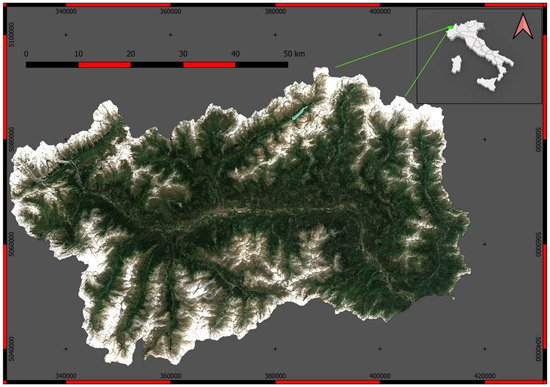
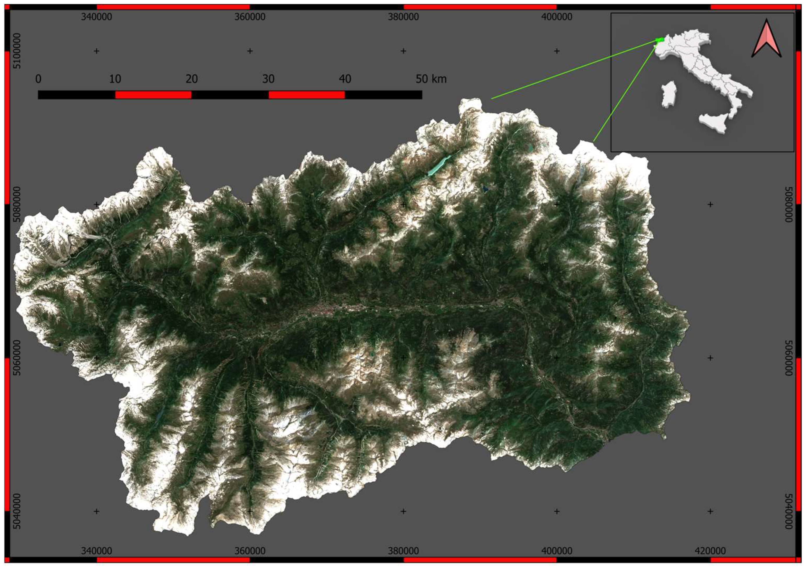
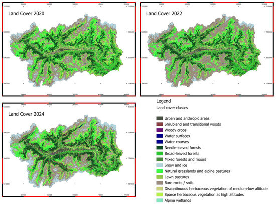
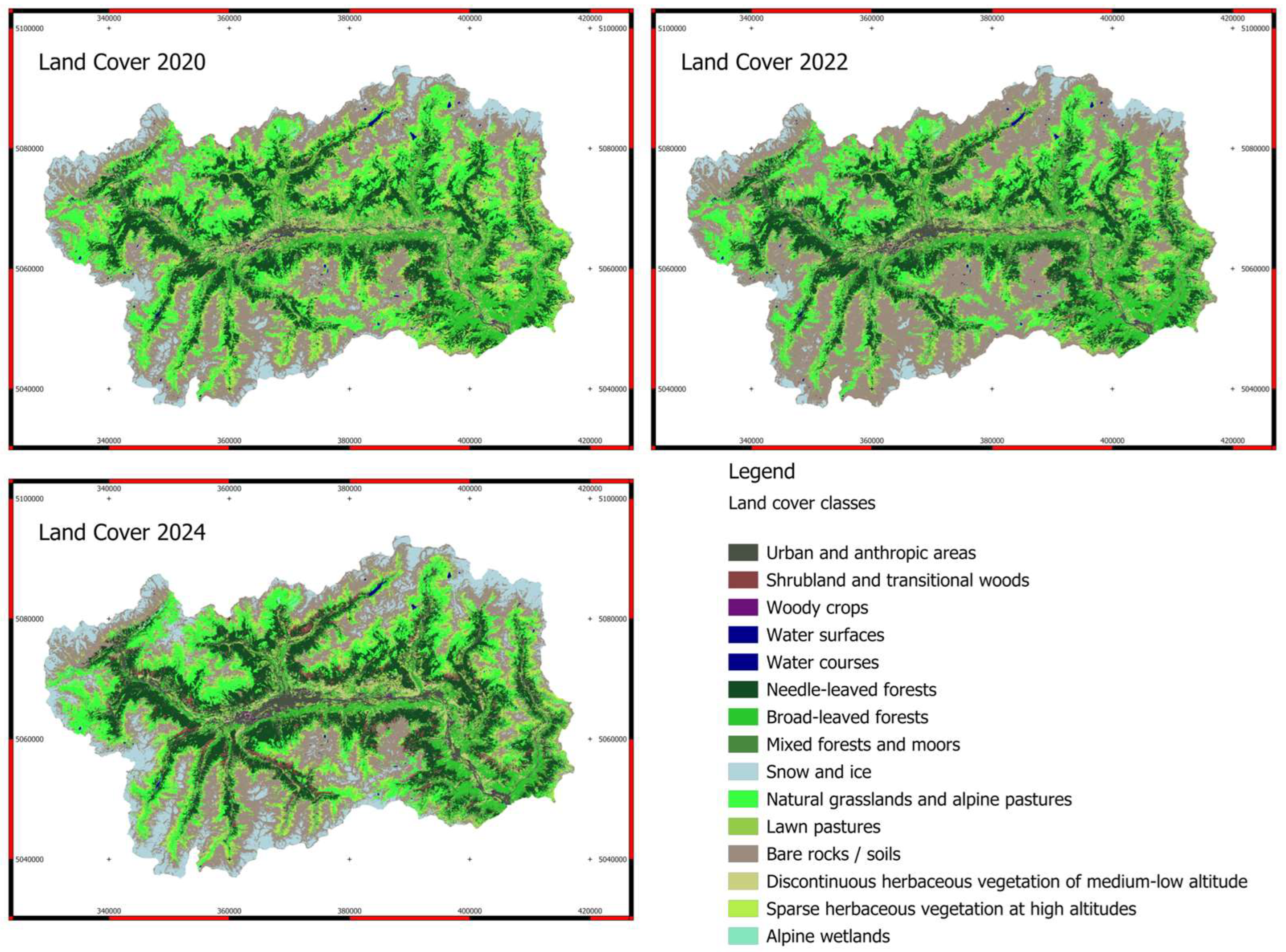
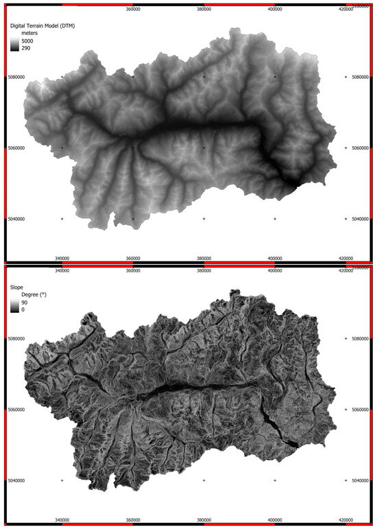
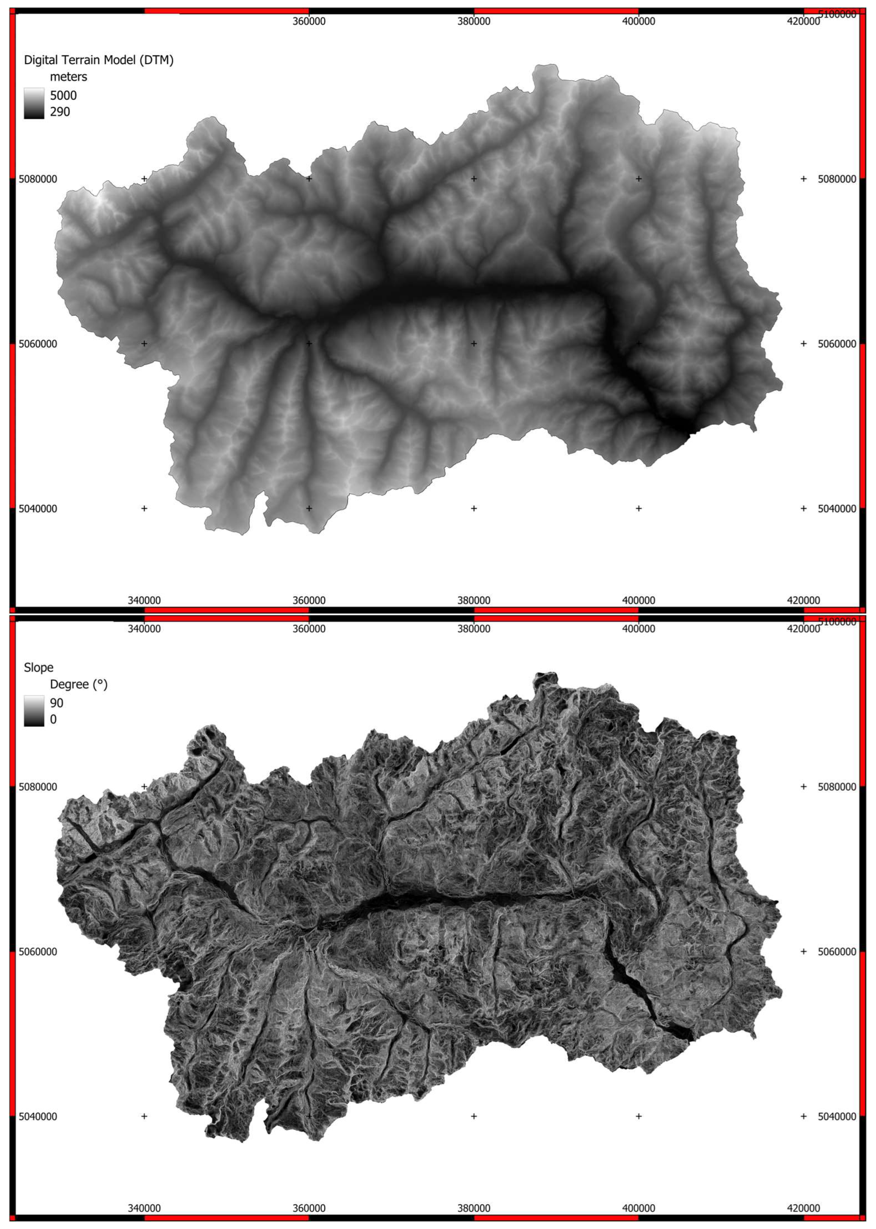
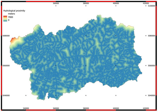
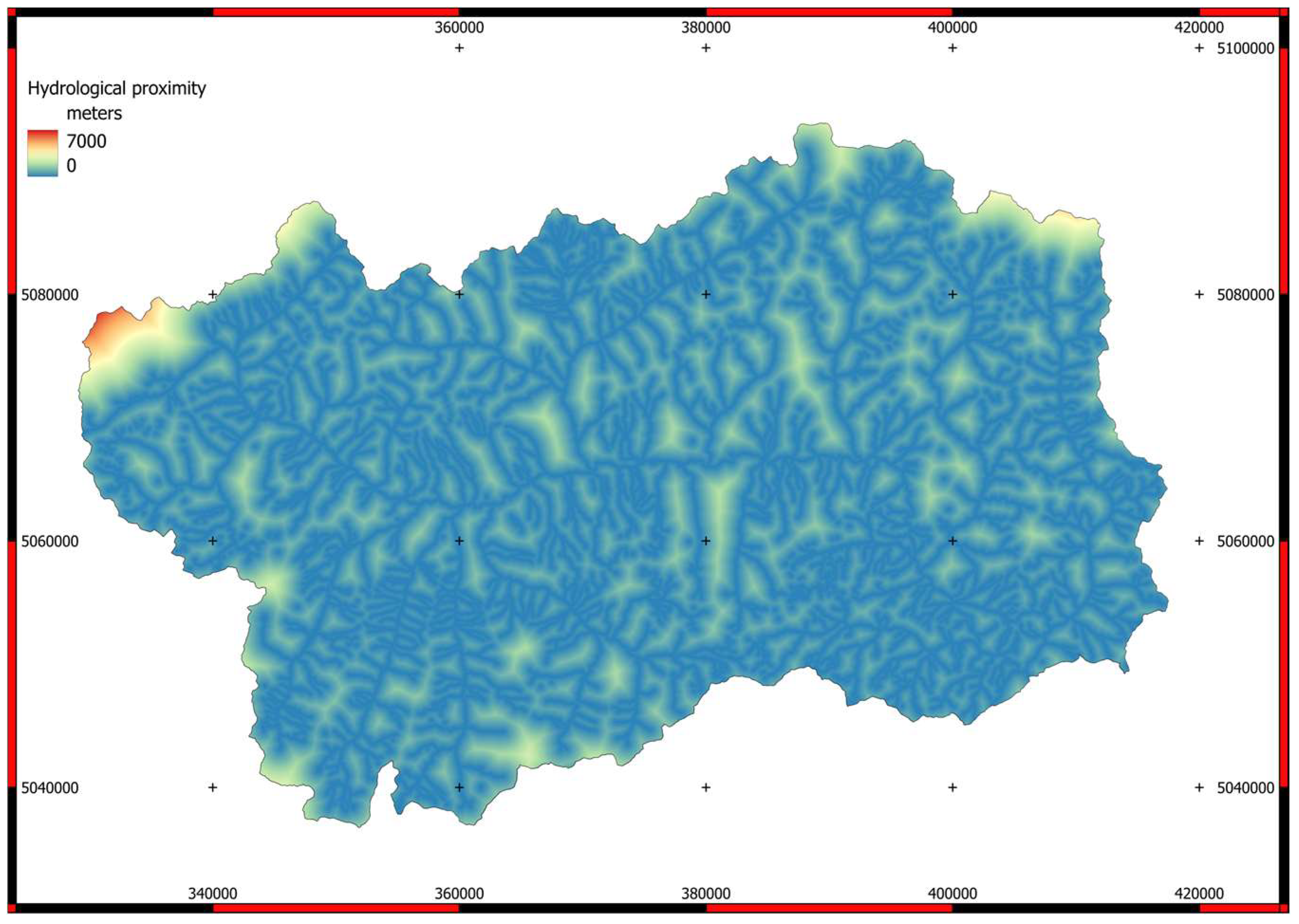
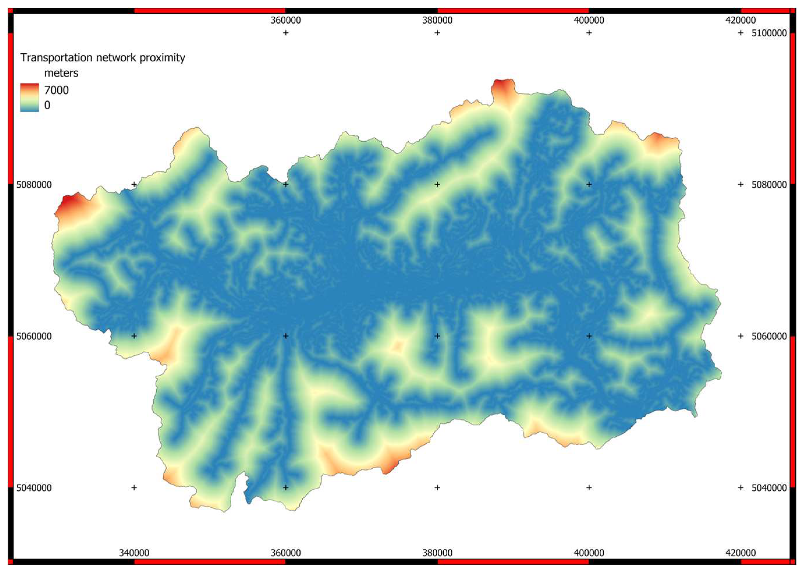
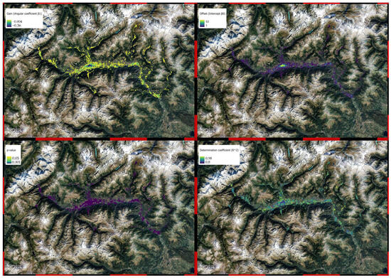
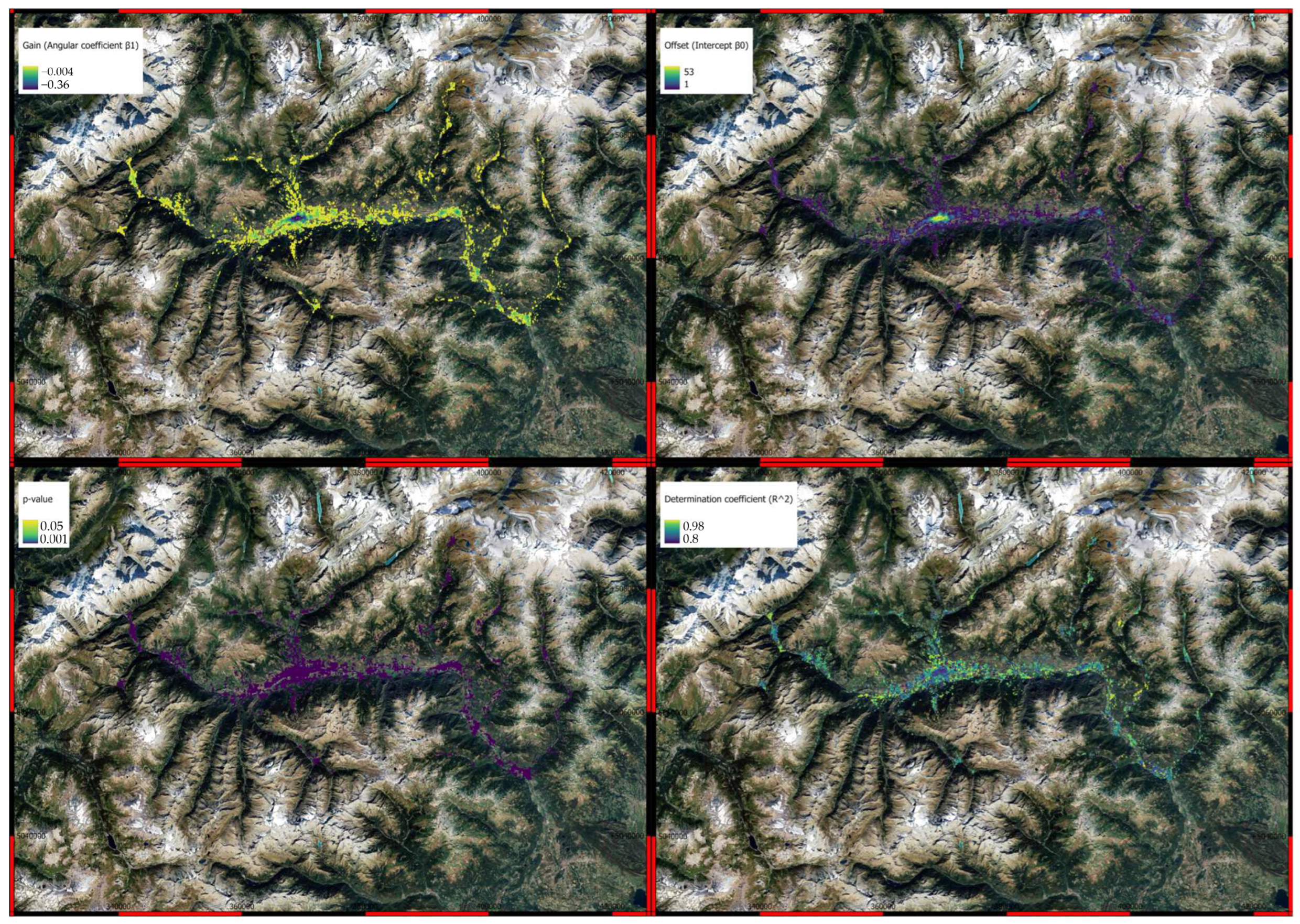
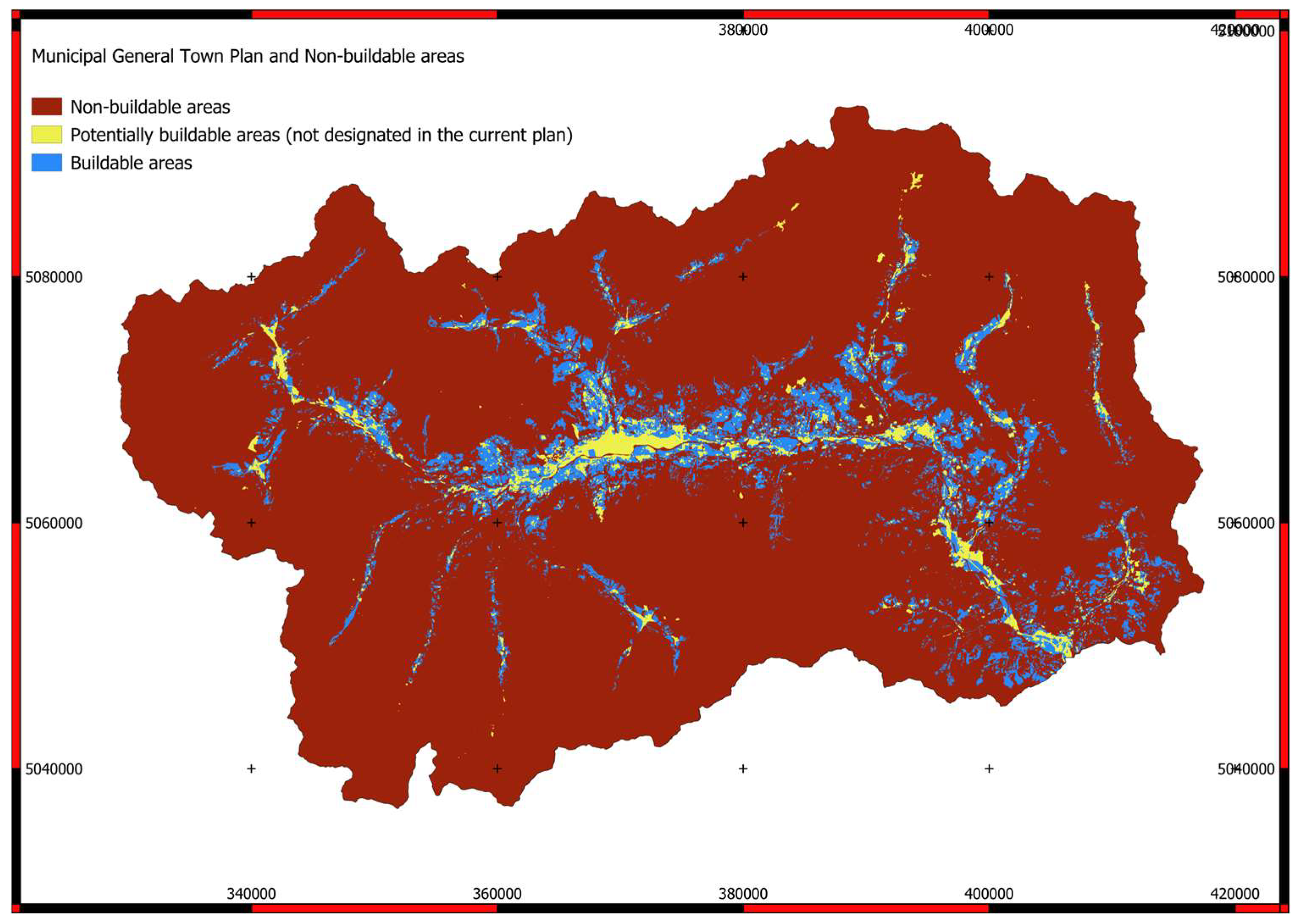
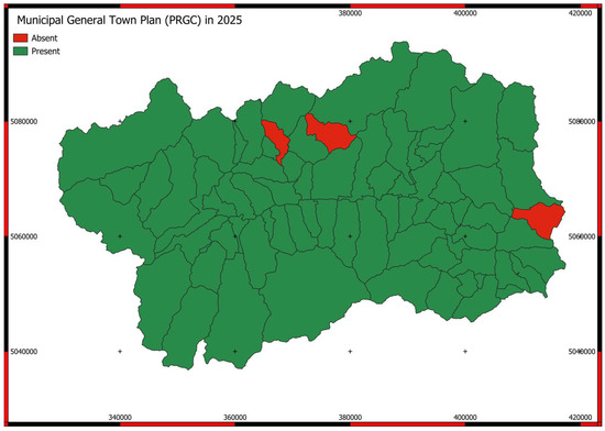
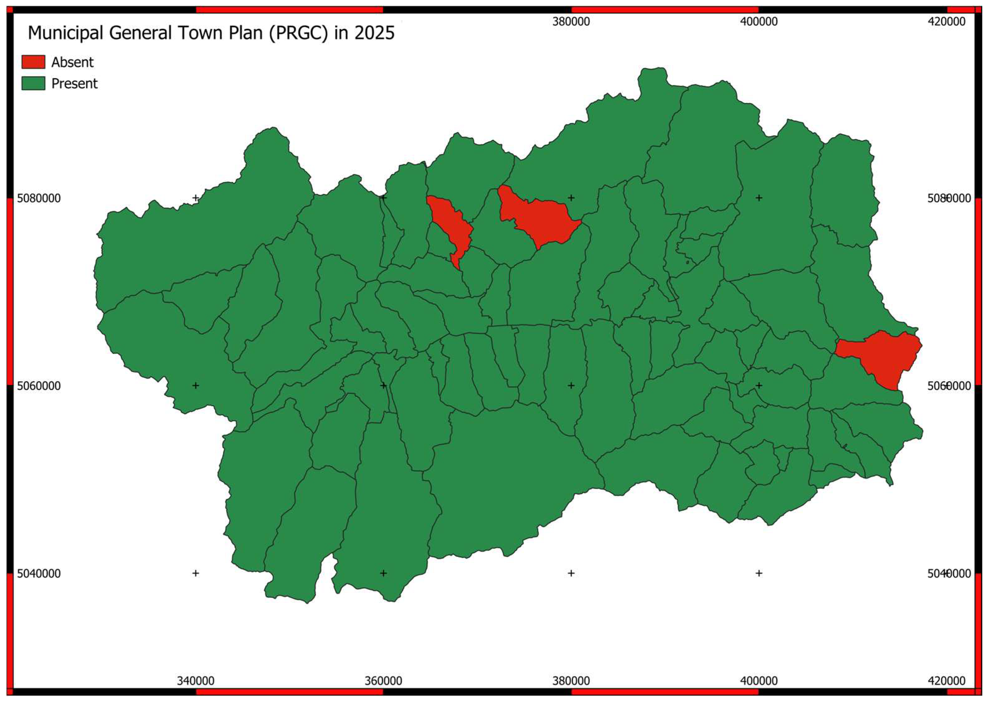
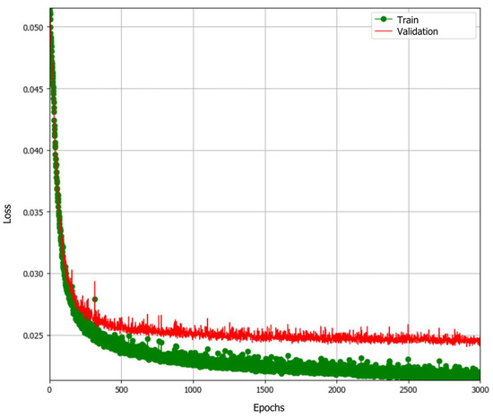
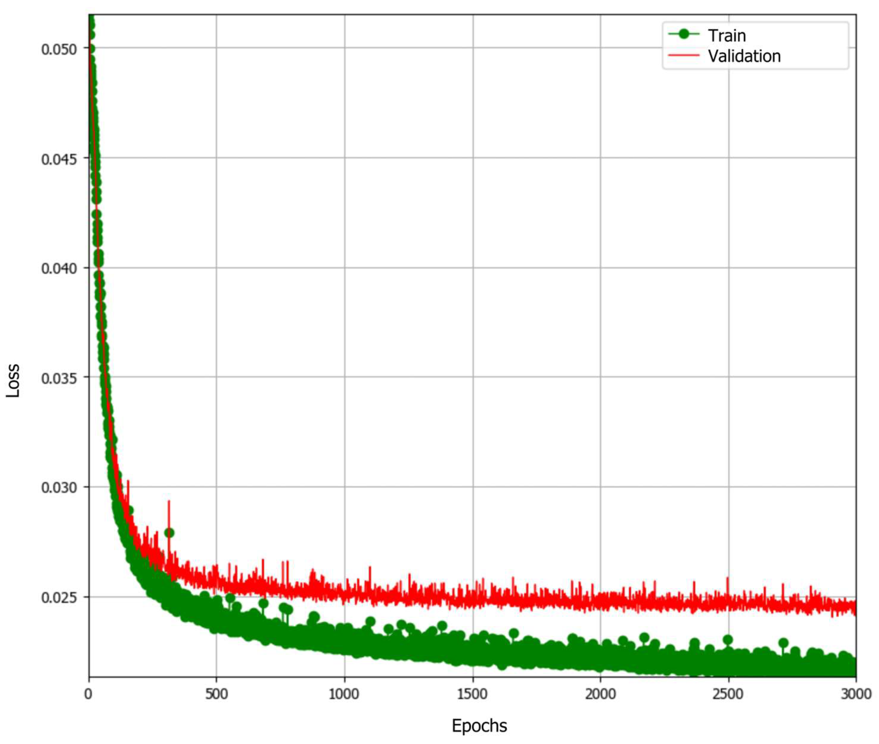
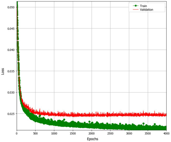
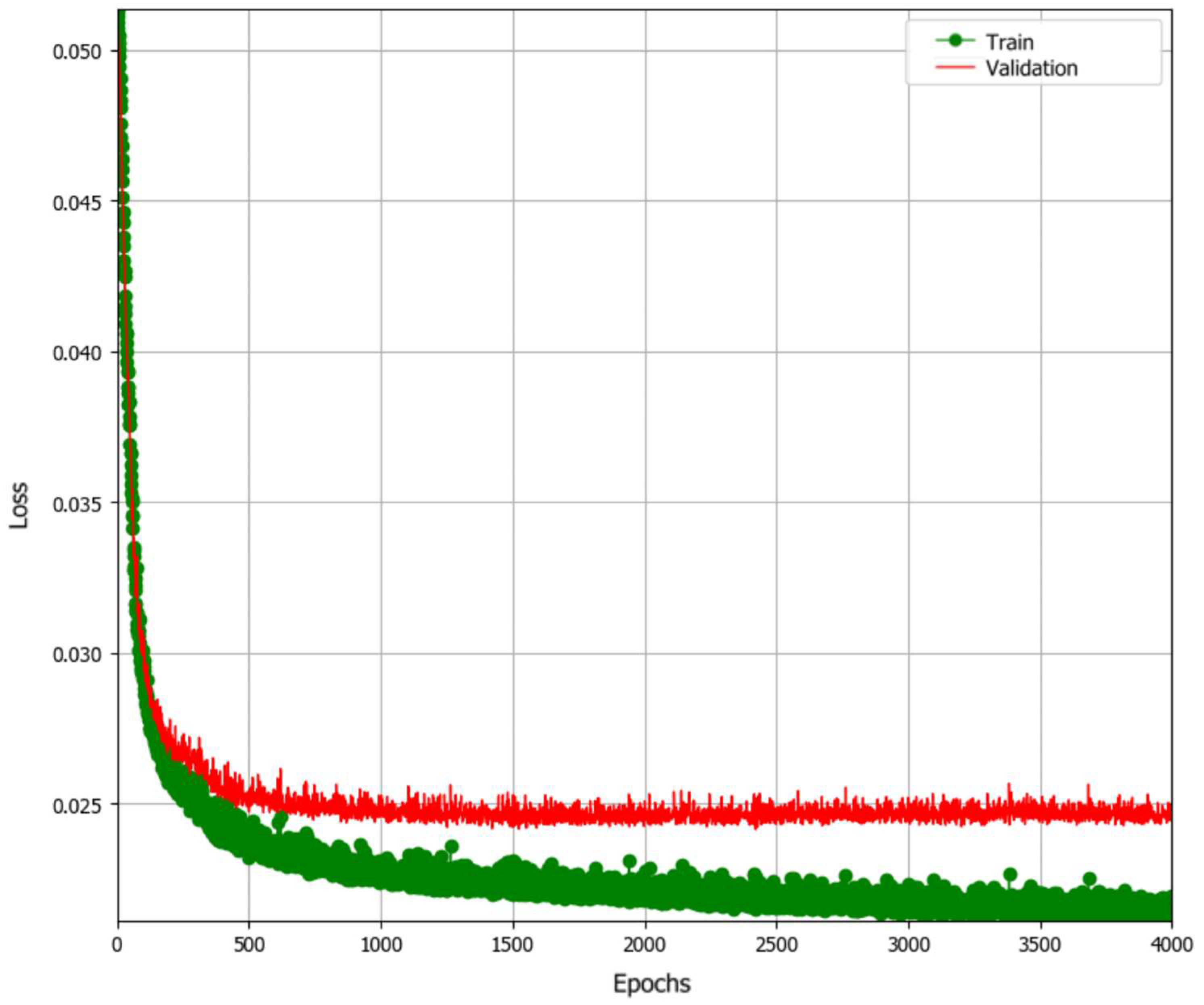
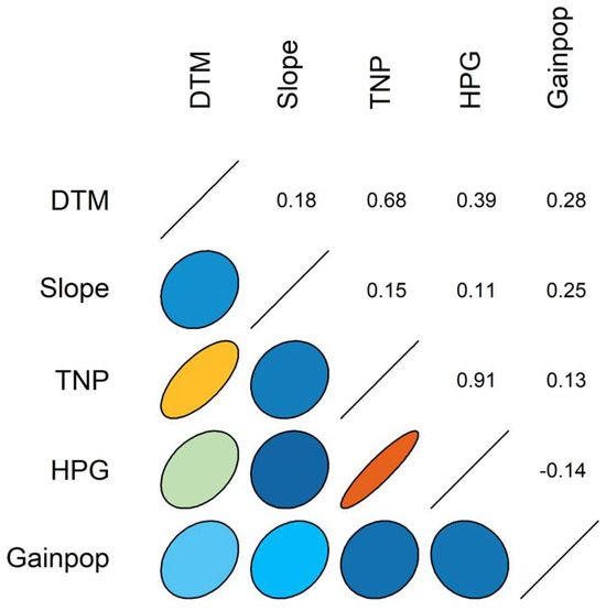
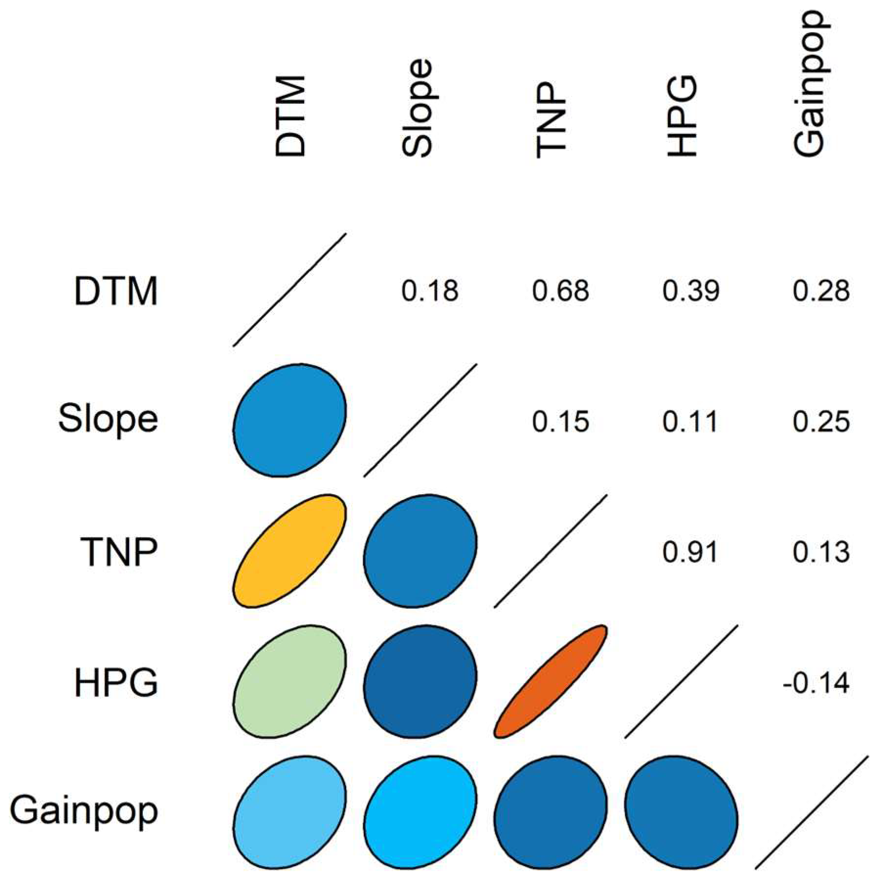
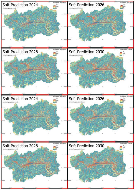
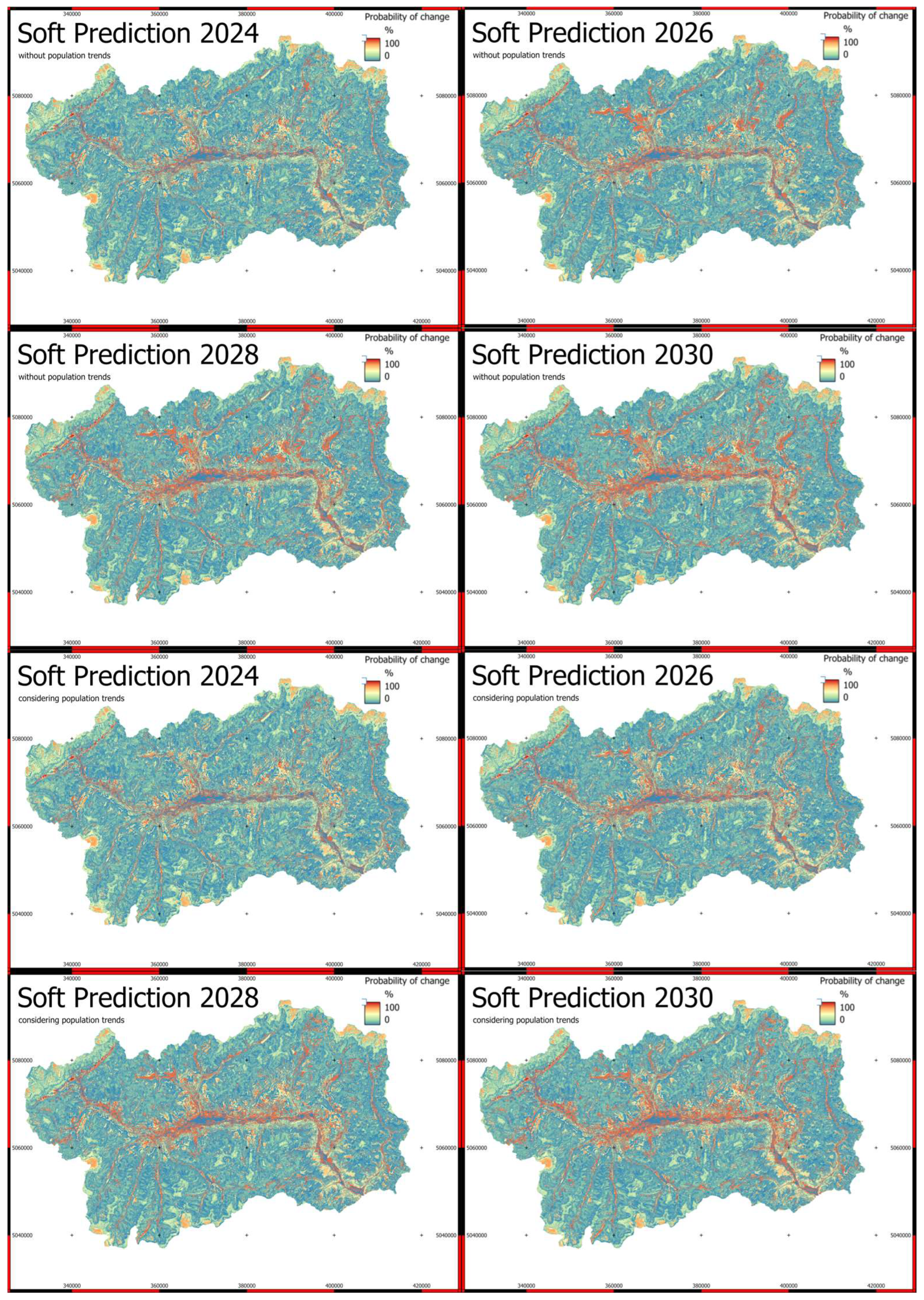
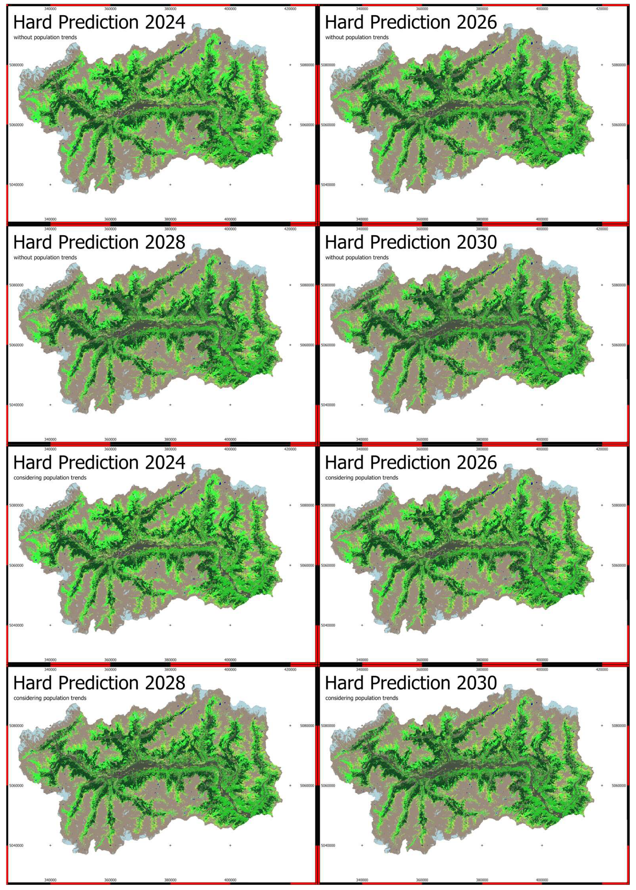
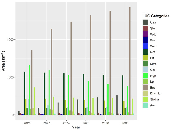
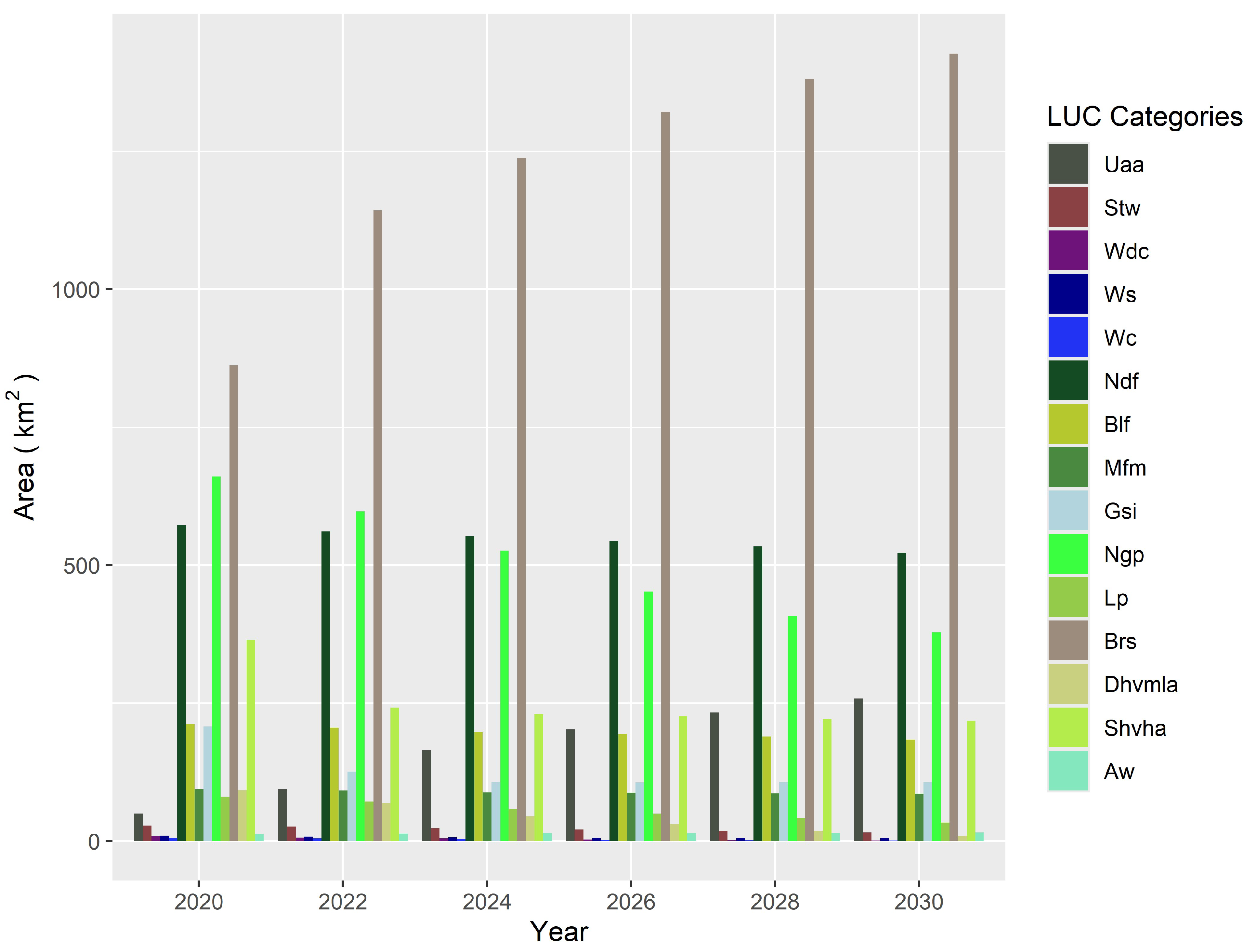
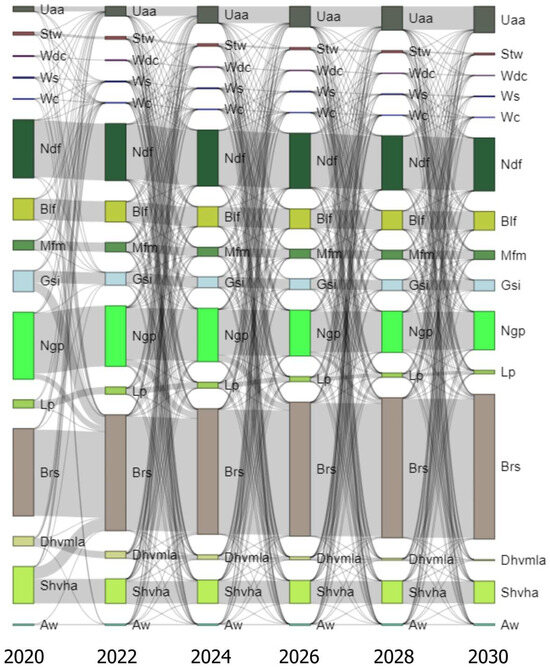
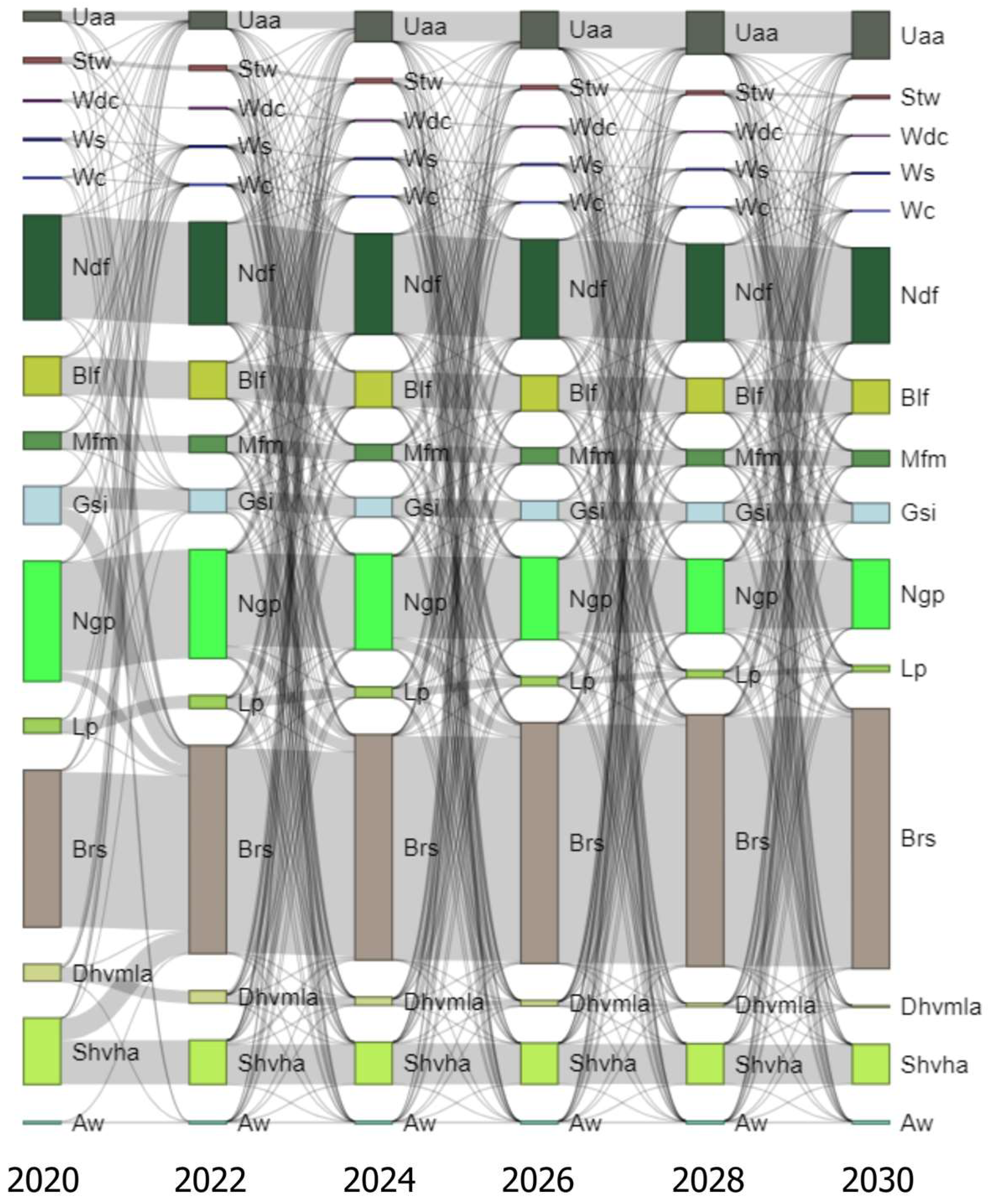
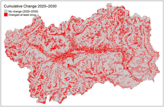
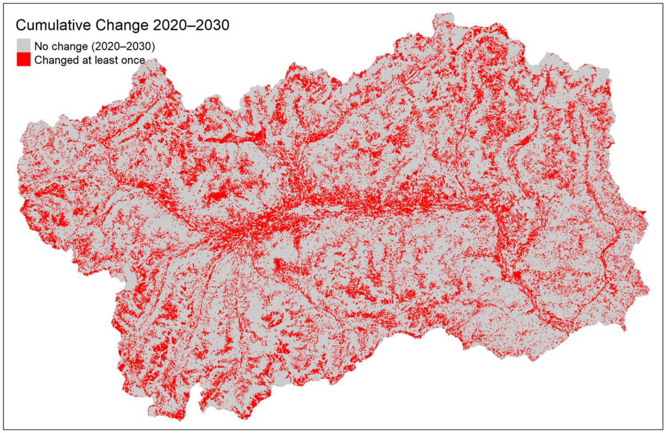

Disclaimer/Publisher’s Note: The statements, opinions and data contained in all publications are solely those of the individual author(s) and contributor(s) and not of MDPI and/or the editor(s). MDPI and/or the editor(s) disclaim responsibility for any injury to people or property resulting from any ideas, methods, instructions or products referred to in the content. |
© 2026 by the authors. Licensee MDPI, Basel, Switzerland. This article is an open access article distributed under the terms and conditions of the Creative Commons Attribution (CC BY) license.