The Mechanism by Which Jobs–Housing Mismatch Affects Urban Land Resource Allocation Efficiency Under External Shocks: An Excess Commuting Perspective

Abstract

Excess commuting reflects the inefficiency of urban land resource allocation, generating additional greenhouse gas emissions and social costs, and has therefore become a central concern in the pursuit of sustainable cities. While exogenous shocks inevitably alter the efficiency of land resource allocation, it remains unclear how such shocks affect overall urban efficiency. To address this gap, this paper proposes a generalized framework for measuring excess commuting that accounts for imbalances between the numbers of jobs and residences. Drawing on mobile signaling big data, we trace the daily commuting patterns of more than 900,000 residents in Beijing, comparing the pre-pandemic period (March–October 2019) with the pandemic period (March–October 2020). The results show that: (1) Excess commuting increased significantly after the outbreak of COVID-19, with the observed average commuting distance (Tact) of the full sample rising from 6267 m to 10,058 m (an increase of 59%), indicating a decline in urban land resource allocation efficiency; (2) A more pronounced center-periphery pattern emerged at the metropolitan scale: the average Jobs–Housing Ratio (JHR) increased from 1.08 to 1.11, and its standard deviation rose from 0.54 to 0.70, with the JHR of central urban areas decreasing by 3% and that of suburban areas increasing by 20%—suggesting a marked increase in commuting distances; (3) Heterogeneous impacts were observed across age groups: the Difference-in-Differences (DID) regression confirmed a significant negative interaction term (Group × COVID-19 = −0.2991 **, p < 0.05), indicating that older adults experienced a greater increase in commuting inefficiency than younger adults. These findings reveal the dynamic mechanisms linking exogenous shocks, jobs–housing mismatch, and urban land resource allocation efficiency and provide policy implications for improving spatial resource allocation in the post-pandemic era.

1. Introduction

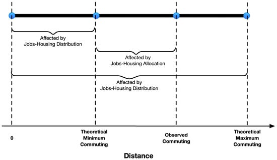
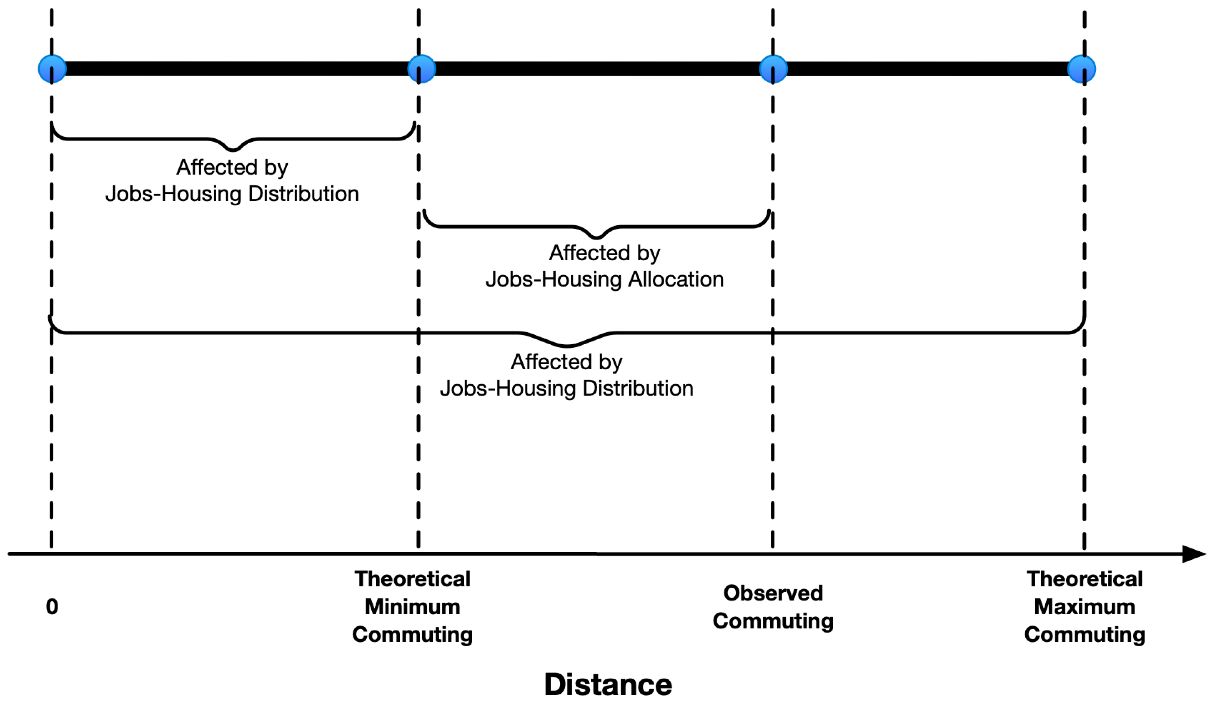
With the expansion of urban areas, an increasing proportion of people live in cities, which are now the hub of human activity and host more than half of the world’s population [1,2]. While agglomeration in the cities provides people with the conveniences they desire, it also entails negative externalities, such as traffic congestion and air pollution [3,4]. Generally, these problems associated with city growth arise because travel demand exceeds the available infrastructure or urban space [5,6]. A large part of the problems can be alleviated by providing larger spaces and improved transportation infrastructure, but it is difficult to significantly change urban structures in a short period of time. Therefore, the jobs–housing distribution is relatively stable in the short term. As a consequence of the land market not always being efficient, the relationship between the efficiency of space utilization and the size of the city is non-linear, with the efficiency of land use first increasing and then decreasing as the city grows [7]. Controlling the expansion of urban boundaries and improving the intensity of the use of existing urban space have therefore become priorities. Many studies have examined how to reduce urban travel demand by improving the efficiency of jobs–housing allocation, which has been considered the most effective countermeasure by planners, researchers, and policymakers [8,9,10], as shown in Figure 1.

Figure 1. The difference in jobs–housing allocation and jobs–housing distribution.

Excess commuting facilitates our analysis of jobs–housing allocation. The concept of excess commuting has been extensively studied to understand how the arrangement of home and work locations affects travel distances, time, and generalized cost, as well as spatial mismatch and commuting efficiency in urban areas [11,12,13,14,15]. Due to the social division of labor and financial constraints, the choice of jobs and residential locations is influenced by population characteristics [16,17]. Additionally, different age groups respond differently to catastrophic events [18,19,20,21,22,23,24,25]. Therefore, investigating the impact of population characteristics on the jobs–housing allocation helps us understand the changes in urban spatial structure and assists in assessing the impact of shocks, as well as developing corresponding recovery policies [26,27]. But studies that focus on the excess commuting of various groups are relatively limited, particularly in terms of changes following external shocks.

To address this research gap, we analyzed the jobs–housing relationship in situations where the number of residences and workplaces is unequal by proposing a generalized framework for calculating excess commuting. By utilizing mobile signaling data to track the jobs–housing choices of 900,000 residents over two consecutive years, the following two scientific questions were addressed: (a) What are the differences in excess commuting among different groups? (b) How does COVID-19 affect the excess commuting of different groups?

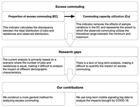
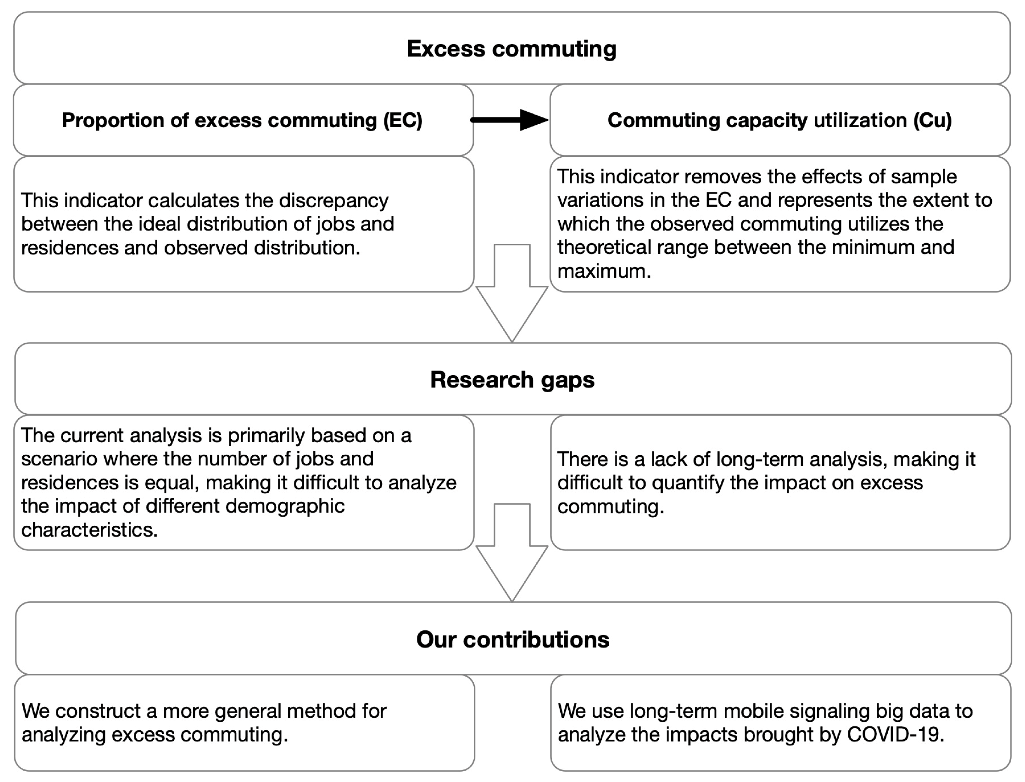
To address these questions, this paper proposes and examines a conceptual mechanism linking external shocks to urban land resource allocation efficiency, as illustrated in Figure 1. We posit that an external shock (such as the COVID-19 pandemic) alters residents’ location preferences and behaviors (e.g., risk aversion). These behavioral shifts, in turn, disrupt the existing jobs–housing spatial match, leading to increased excess commuting. The rise in excess commuting signifies that a greater amount of urban space and time resources are wasted on unnecessary travel rather than being allocated to productive activities or personal welfare. This ultimately manifests as a decline in urban land resource allocation efficiency at the systemic level. Furthermore, this study specifically investigates how this mechanism disproportionately affects different demographic groups, particularly older adults, due to their distinct risk perceptions and adaptability. Our core contributions are shown in Figure 2. Compared to previous studies, (a) we compared the differences in jobs–housing allocations among different groups, providing a new dimension for evaluating jobs–housing balance. (b) We optimized the analytical framework for excess commuting, expanding its application scenarios. (c) Our analysis relies on mobile signaling big data, offering a large sample size and reflecting residents’ revealed preferences.

Figure 2. Filling the current research gaps.

This paper adopts excess commuting as a central measure of urban land resource allocation efficiency. Unlike traditional land use efficiency indicators, which emphasize static and supply-oriented metrics such as floor–area ratio or development intensity, excess commuting provides a dynamic and behavior-oriented perspective. Comparing observed commuting with the theoretical optimum reveals the efficiency losses associated with jobs–housing mismatches and reflects whether land and space are used rationally under minimal commuting costs. Furthermore, excess commuting captures hidden costs, such as energy use, carbon emissions, congestion, and welfare loss, that conventional metrics overlook, while also enabling heterogeneity analysis across demographic groups. In this sense, excess commuting is not only a tool for studying jobs–housing balance but also an effective extension for evaluating urban land use efficiency, especially under external shocks like COVID-19 that reshape spatial interactions and resource allocation patterns. To address the aforementioned research gaps and answer the two scientific questions, this paper is structured as follows: Section 2 systematically combs the existing studies on residents’ jobs–housing location selection behaviors and excess commuting calculation methods, further clarifying the theoretical basis and research limitations of this study. Section 3 proposes a generalized excess commuting measurement framework that accommodates jobs–residences imbalance and introduces the difference-in-differences (DID) approach, jobs–housing ratio (JHR), and Self-Containment of Employment (SCE) used to analyze spatial causes and group differences, while also describing the study area (Beijing) and mobile signaling big data source. Section 4 presents the empirical findings, including the heterogeneous changes in excess commuting across age groups before and during the COVID-19 pandemic, the spatial causes of these changes (based on JHR and SCE), and the DID estimation results of the pandemic’s impact on different groups. Section 5 interprets the empirical results, explores the mechanisms linking exogenous shocks, jobs–housing mismatch, and urban land resource allocation efficiency, and compares the findings with existing literature. Finally, Section 6 summarizes the theoretical contributions, policy implications, and limitations of the study.

2. Literature Review

Excess commuting is used to analyze the jobs–housing balance [15], but unlike indices such as the jobs–housing ratio, which focus on the study of jobs–housing distribution, the research on excess commuting emphasizes a theoretical scenario for measuring efficiency: it calculates the potential for commuting optimization assuming that the current spatial distributions of homes and jobs are fixed but that residents could be reassigned to different jobs and homes within that existing stock. This framework does not imply that individuals have no choice in reality but rather seeks to quantify the efficiency of the outcome of their collective choices against a theoretical optimum given the urban structure. In this section, we conduct a literature review on residents’ jobs–housing choice behaviors, and the research methods of excess commuting.

2.1. Review of Jobs–Housing Location Selection

Due to the rapid development of transportation, the dynamic jobs–housing balance with appropriate commuting distances can also be accepted based on individual characteristics [28]. Consequently, the demographic and socio-economic characteristics of workers, such as income, age, race, educational attainment, and self-selection [29], are often considered important factors influencing residents’ commuting travel behavior. Spatial characteristics can also influence the balance between jobs and housing through the decentralization of urban populations and the relocation of job opportunities [30]. Commuting often results in stress due to its unpredictability and the perceived loss of control [31,32]. People might change their residential location choice or workplaces to adapt to worsening congestion and to maintain an acceptable commuting distance or commuting time [33,34,35].

Age can also influence residents’ location choices. However, age itself is not a direct factor impacting travel behavior; instead, it acts as a representative for other age-related changes, such as shifts in household dynamics, changes in employment, or health decline [36]. Older individuals appear to be more risk-averse or have increased concerns about personal safety compared to younger ones; as a result, older cyclists place a higher emphasis on their safety [16,17]. Regarding preferences for public transportation choices, elderly individuals tend to prefer public transportation more than younger individuals, especially when the service quality is enhanced [37]. Older travelers place more emphasis on the “ticket price”, whereas younger travelers value aspects like avoiding transfers and punctuality [38].

2.2. Review of Excess Commuting Method

Numerous studies on excess commuting have described it as the additional or unnecessary travel to work caused by the varied locations of homes and workplaces that shape the urban environment [11,39]. Therefore, some consider it an extension of the jobs–housing balance [40]. In quantitative terms, excess commuting represents the gap between the observed average commuting costs and the theoretical minimum average commuting costs in an urban area [41]. Unlike metrics such as the jobs–housing ratio and the Self-Containment of Employment, which analyze the jobs–housing relationship at a grid level, excess commuting depicts commuting behavior at the city level.

White (1988) used linear programming to calculate the proportion of excess commuting by comparing the minimum commuting time to the observed commuting time when the places of residence and work are determined [11]. Excess commuting has provided the foundation for various benchmarks and indices to analyze the efficiency of commuting and land use configurations in urban areas; this has led to several enhancements to the linear optimization method [15,42]. The idea of a theoretical average maximum commute has been proposed as a way to gauge the spread and extent of urban sprawl, assisting in the evaluation of commuting efficiency in urban regions [12,43].

The cost matrix within the excess commuting framework mainly includes two types: time and distance. The time matrix is used to study the characteristics of residents’ commuting behavior, with time being related not only to distance but also to spatial features and individual travel preferences. Distance, on the other hand, can be used to analyze issues such as urban structure, energy consumption, and environmental pollution [44]. When the aim of the study is to assess the changing urban form over different points in time, distance is a more appropriate measure to use than time [41]. While Euclidean distance underestimates the observed distances traveled between zones, it does so roughly equally across all routes in the network, indicating that the measure is a good proxy for measuring relative commuting cost between zonal units [45].

2.3. Summary

Although many studies have answered how age differences affect residents’ jobs–housing choices, no study has yet addressed how age differences impact the efficiency of jobs–housing allocation at the urban level. Current research on excess commuting, although providing a framework for analyzing urban-level jobs–housing allocation, still lacks the capability to analyze excess commuting related to unequal numbers of jobs and residences. For instance, while men may have fixed workplaces, their choice of residence spans all available homes in the city, meaning the number of workplaces and residences is not equal. Additionally, urban vacancy rates are not always zero, making the imbalance between the number of jobs and residences a more general case.

3. Method

To analyze the issue of jobs–housing balance at the city level across different demographics, we first propose a more general excess commuting method and use this method to analyze the differences in excess commuting among different age groups before and during the COVID-19 pandemic. Then, we use the jobs–housing ratio (JHR) and Self-Containment of Employment (SCE) to explore the geographical reasons for the change in excess commuting. Finally, we use the difference-in-differences method to analyze the impacts of COVID-19 on excess commuting for groups with different characteristics, as shown in Figure 3.

Figure 3. Analytical framework of this paper.

3.1. Measurement of Excess Commuting

To overcome the limitation of standard excess-commuting (EC) models that implicitly assume balanced job–housing totals, we allow the numbers of jobs and workers to differ by introducing slack variables into a linear-programming formulation. Let origins (residential zones) be indexed by $i=1,2,\dots ,n$ and destinations (employment zones) by $j=1,2,\dots ,m$. Denote the number of workers residing in the origin $i$ by $O_i$, the number of jobs in the destination $j$ by $D_j$, the generalized travel cost (time or distance) between $(i,j)$ by $C_{ij}$, and the flow of workers assigned from $i$ to $j$ by $x_{ij}$. We compute theoretical lower and upper bounds on average commuting cost by solving:

$$Minimize:T_{\mathrm{m}\mathrm{i}\mathrm{n}}={\displaystyle \frac{1}{W}}\sum _{i=1}^n\sum _{j=1}^m{C}_{ij}{x}_{ij}$$

(1)

$$Maximize:T_{\mathrm{m}\mathrm{a}\mathrm{x}}={\displaystyle \frac{1}{W}}\sum _{i=1}^n\sum _{j=1}^m{C}_{ij}{x}_{ij}$$

(2)

Subject to:

$$\sum _{i=1}^n{x}_{ij}+{\alpha }_j=D_j, \forall j=\mathrm{1,2},\dots ,m$$

(3)

$$\sum _{j=1}^m{x}_{ij}+{\beta }_i=O_i, \forall i=\mathrm{1,2},\dots ,n$$

(4)

$${\alpha }_j\ge 0,{\beta }_i\ge 0,x_{ij}\ge 0,\forall i,j$$

where $W$ denotes the total number of commuters in the study area, ${\alpha }_j$ and ${\beta }_i$ are slack variables associated with the employment zone $j$ and residential zone $i$, respectively.

Following White (1988) [11], the proportion of excess commuting is shown in Formula (5):

$$EC={\displaystyle \frac{T_{act}-T_{min}}{T_{act}}}\times 100$$

(5)

where $T_{act}$ is the observed average commuting time (or distance). Building on this framework, Horner (2002) defines commuting capacity utilization [12], as shown in Formula (6), which measures the extent to which the observed commuting utilizes the theoretical range between the minimum and maximum possible commuting.

$$C_u={\displaystyle \frac{T_{act}-T_{min}}{T_{max}-T_{min}}}\times 100$$

(6)

The $C_u$ indicator measures the extent to which the observed commuting pattern utilizes the full theoretical range between the most efficient ($T_{min}$) and least efficient ($T_{max}$) spatial arrangements. $T_{\mathrm{m}\mathrm{i}\mathrm{n}}$ corresponds to an assignment that, given the fixed spatial distributions of workers and jobs, matches each worker to an available job so as to minimize aggregate travel cost; $T_{max}$ provides the opposite bound under the same feasibility constraints. The approach treats residential and job locations as homogeneous with respect to preferences—i.e., reassignment does not reduce individual utility—so that $T_{\mathrm{m}\mathrm{i}\mathrm{n}}$ and $T_{\mathrm{m}\mathrm{a}\mathrm{x}}$ serve as theoretical lower and upper limits on the achievable average commuting cost. In this framework, the spatial distributions of workers ($O_i$) and jobs ($D_j$) are treated as fixed constraints. The linear programming model then explores how workers could be hypothetically rearranged among the available jobs to either minimize or maximize the total commuting cost. This simulates the collective commuting choices available to the population under the current urban form. The difference between the actual commuting pattern and the theoretical minimum ($T_{min}$) thus represents the ‘excess’ commuting that arises from the real-world choices and constraints of residents (e.g., personal preferences, housing affordability, information asymmetry) that prevent the system from achieving the most spatially efficient outcome. Therefore, excess commuting not only reflects the additional travel costs at the individual level but also reveals the loss of urban land resource allocation efficiency at the aggregate level. When actual commuting deviates significantly from the theoretical optimum, it implies that more spatial resources are being wasted on unnecessary commuting.

Our general framework supports subgroup-specific analysis of the jobs–housing relationship. To enable meaningful comparisons, we employ the capacity-utilization index $C_u$, a unit-free, standardized analog of EC that scales the realized commute by the feasible range implied by the opportunity set [12]—i.e., between the theoretical minimum $T_{min}$ and maximum $T_{max}$. Within a single city, $C_u$ likewise mitigates comparability problems across subgroups, placing different populations on a common scale. Our contribution is to operationalize this standardized comparison and thereby assess subgroup disparities in jobs–housing balance within a consistent, city-wide benchmarking framework.

3.2. Difference-in-Differences (DID) Approach

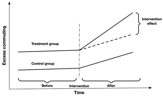
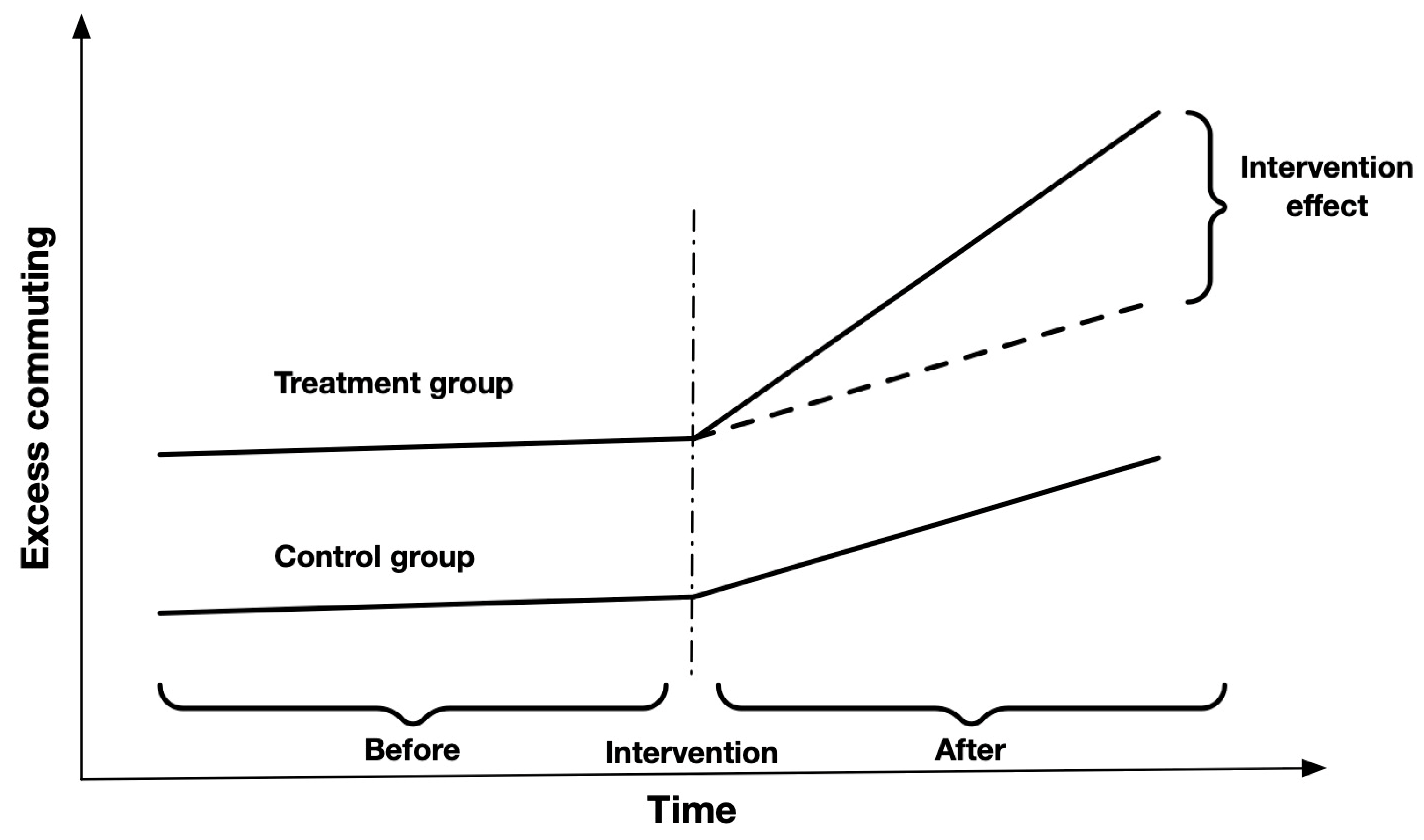
The DID approach is a statistical technique used in econometrics and social sciences to estimate the causal effect of a specific intervention. This method is particularly useful in observational studies where random assignment is not possible. The DID approach relies on a quasi-experimental design and compares the changes in outcomes over time between a population that is enrolled in a program (the treatment group) and a population that is not (the control group), as shown in Figure 4. By comparing the difference in outcomes of these two groups before and after the intervention, DID attempts to control for unobserved factors that could influence the results.

Figure 4. The graphic representation of the difference-in-differences regression.

The key assumption of the DID approach is the “parallel trends assumption”. This means that, in the absence of the treatment, the treatment and control groups would have followed the same trend over time. We ensure that the parallel trends assumption holds, meaning that the treatment and control groups had similar outcome trends before the intervention. We adopt the addition of time-fixed effects in the model, along with the ADF stationarity test, to verify whether the control group and the treatment group have the same trend before the shock in this study. The solid line shows the observed path; the dashed line shows the counterfactual path—projected under the parallel-trends assumption—if the shock had not occurred.

The baseline DID model can be represented by the following regression equation:

$$Y_{it}=\alpha +\beta Treatmen{t}_i+\gamma Pos{t}_t+\delta Treatmen{t}_i\ast Pos{t}_t+{\epsilon }_{it}$$

(7)

where

$Y_{it}$ is the outcome of excess commuting for the unit $i$ at time $t$.

$Treatmen{t}_i$ is a binary variable indicating whether the unit $i$ is in the treatment group (1 if treatment, 0 if control).

$Pos{t}_t$ is a binary variable indicating the time period (1 for post-treatment periods, 0 for pre-treatment periods).

$\alpha$ is the constant term (intercept).

$\beta$, $\gamma$, and $\delta$ are the coefficients to be estimated.

$\delta$ is the DID estimator, representing the average treatment effect.

${\epsilon }_{it}$ is the error term.

3.3. Self-Containment of Employment (SCE) and Jobs–Housing Ratio (JHR)

The jobs–housing ratio was used to examine the spatial pattern of jobs and residents [46], which is calculated using Formula (8):

$${JHR}_i={\displaystyle \frac{J_i}{H_i}}$$

(8)

where

${JHR}_i$ represents the jobs–housing ratio in the area $i$, $J_i$ represents the number of workplaces in the area $i$, $H_i$ represents the number of residences in the area $i$ (which is not equal to 0).

SCE measures the degree to which a locality provides employment opportunities for its residents. High SCE plays an important role in reducing travel demand and promoting environmentally friendly modes of transportation [47]. Unlike the JHR, the SCE places emphasis on residents who both live and work within the same area, thereby incorporating the notion of jobs–housing allocation efficiency. In prior studies, this indicator was measured as the ratio of the number of jobs to the number of resident workers in a given zone, as shown in Formula (9). By replacing the denominator with the number of residences, this ratio can also be used to analyze the richness or abundance of residences in that region, as shown in Formula (10):

$${SCE}_{H,i}={\displaystyle \frac{{MATCH}_i}{H_i}}$$

(9)

$${SCE}_{J,i}={\displaystyle \frac{{MATCH}_i}{J_i}}$$

(10)

where

${SCE}_{H,i}$ represents the jobs–housing match for residents in the area $i$.

${SCE}_{J,i}$ represents the living match index for workers in the area $i$.

${MATCH}_i$ is the total number of people whose workplace and residence are both in the area $i$.

Since we focus on the relative changes in SCE for different groups, we calculate $RSCE$ (the ratio of SCE for different categories).

$$RSCE={SCE}_{J,i,sub\_group\_1}/{SCE}_{J,i,sub\_group\_2}$$

(11)

This can eliminate the impact brought by the differences in $H_i$ or $J_i$, and we only need to compare the values of ${MATCH}_i$.

3.4. Study Area and Data

3.4.1. Study Area

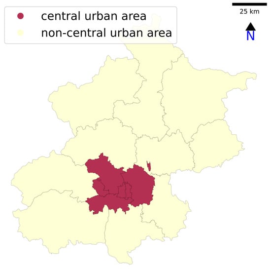
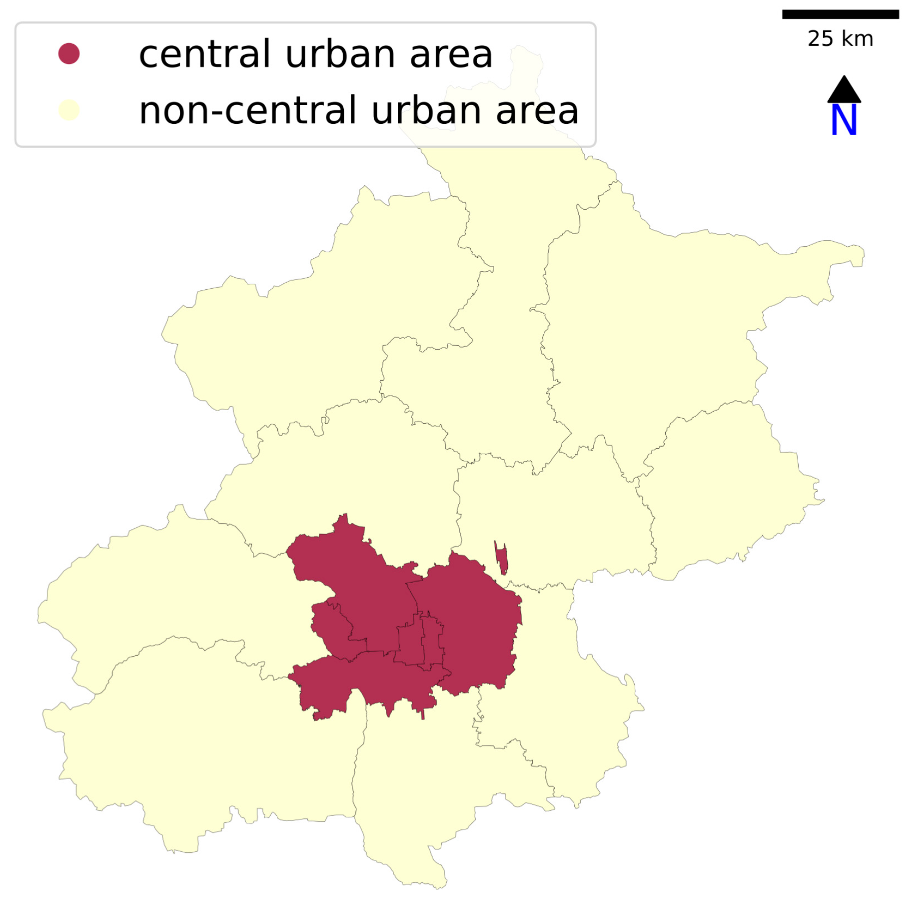
As the capital of China, Beijing covers an area of approximately 16,800 square kilometers and is divided into 316 jiedao, the smallest administrative units in the country. The allure of urban living, educational opportunities, and job prospects attracts people from across China to the capital city. In 2020, the city had a total population of approximately 21.84 million, according to the seventh population census of the country. The central urban area of Beijing includes six districts, namely Xicheng, Dongcheng, Shijingshan, Fengtai, Haidian, and Chaoyang [48], as shown in Figure 5. Notably, 60 percent of the city’s permanent population resides in the city’s central area, resulting in a concentrated population [49].

Figure 5. Study area.

Beijing’s rapid urbanization, coupled with its booming population, has altered its natural landscape, resulting in environmental challenges such as air pollution and urban heat islands [50]. To deal with these environmental concerns and protect its surroundings, numerous manufacturing industries have been relocated outside the city limits. Additionally, the outbreak of the pandemic has changed people’s location choice preferences and travel behaviors, including an increase in the proportion of residents working from home, a reduction in non-essential travel, and relocation to areas with lower infection risks [51], which has exacerbated the separation of workplaces from residences in urban areas. Therefore, we have selected Beijing as the research area, and treat the COVID-19 pandemic as an exogenous shock in this study.

3.4.2. Data Source

We utilized mobile phone signaling data from Beijing, spanning from March to October in both 2019 and 2020, covering eight months of data. The 2019 data serves as the pre-pandemic baseline, while the 2020 data captures mobility patterns during the initial and ongoing phases of the COVID-19 pandemic. The descriptive information of the data is presented in Table 1. The binary age categorization (20–40 and 40–60) is justified on both theoretical and practical grounds. Theoretically, these groups represent distinct life-course stages with differing mobility, stability, and risk perceptions, which are crucial for heterogeneous shock responses. Practically, individuals over 60 are largely excluded, as a significant portion are retired, and their non-commute travel would confound our jobs–housing analysis. While we acknowledge the importance of gender, education, and occupation, these attributes are unavailable in our mobile signaling data. Our study thus provides a foundational analysis of a major demographic divide, establishing a clear empirical pattern for future research to disentangle with richer socio-economic data.

Table 1. Distribution of people in categories for analysis.

Variable	Number of People	Percentage
Young adults (20–40)	544,636	59%
Older adults (40–60)	382,246	41%
Total	926,882	100%

Mobile phone signaling data primarily comprises communication timestamps between users and base stations, along with the coordinates of these base stations. By employing the operator’s multi-base station weighting algorithm, the coordinates of individuals’ locations can be recognized. We identify “stay points” as locations where individuals linger for over 30 min. To define a stable residence or workplace from these stay points, we implemented the following procedure: First, we required an individual to have a consistent stay point at a given location on a majority of weekdays over the entire eight-month observation period to ensure stability. Then, for these stable locations, the workplace was determined as the one with the longest cumulative stay duration during weekday hours from 5 a.m. to 8 p.m., and the residence as the one with the longest cumulative stay duration during nighttime hours from 8 p.m. to 5 a.m. This two-step process ensures that we capture long-term, habitual locations rather than temporary visits. However, this approach may not accurately capture the patterns of night-shift workers, whose commuting behavior and activity locations could appear reversed. We acknowledge this as a limitation of our data and methodology. While it is challenging to precisely isolate this group in our dataset, the proportion of night-shift workers in the overall workforce is generally small. Therefore, we do not expect this to significantly alter the aggregate trends observed in our study, though it may introduce some noise at the individual level.

Additionally, mobile phone signaling data also includes a plethora of individual attributes and travel information. The use of mobile phone signaling data offers several advantages: First, when compared to survey data, this dataset not only reflects the revealed preferences of residents but also mitigates biases arising from information withholding or varied interpretations of survey questions [52]. Second, this dataset includes not only a large number of samples but also records their long-term travel behaviors, which is helpful for us to conduct time-series analysis [53].

During the computation of commuting distances, we use the “jiedao” as the unit of analysis. We assume that the commuting distance between jiedaos is the distance between the centroids of the two jiedaos [15], and if both the workplace and residence are located in the same jiedao, the commuting distance is considered to be zero. It is important to note that jiedaos, as administrative units, are not uniform in size or population. Their area and resident count can vary considerably across the city. This heterogeneity is a common characteristic in urban spatial analysis based on administrative boundaries. However, the jiedao serves as the fundamental statistical and planning unit in Chinese cities, ensuring data availability and policy relevance. To mitigate potential biases arising from the modifiable areal unit problem, our commuting cost matrix is calculated as the distance between jiedao centroids. This approach provides a standardized measure of separation between zones, which is widely adopted in excess commuting studies [12,15,45]. While using a finer-grained grid could be an alternative, the jiedao level offers a meaningful scale for analyzing jobs–housing relationships and formulating neighborhood-level policies.

During data extraction and analysis, we primarily employed Hive SQL 3.3.1 and subsequently processed the outputs in Python 3.13.1. The analytical workflow relied on NumPy 2.3.4 and GeoPandas 1.1.1, visualization was conducted with Matplotlib 3.10.7, and model estimation and inference were implemented using statsmodels.

4. Results

4.1. Heterogeneous Excess Commuting Changes Across Social Groups

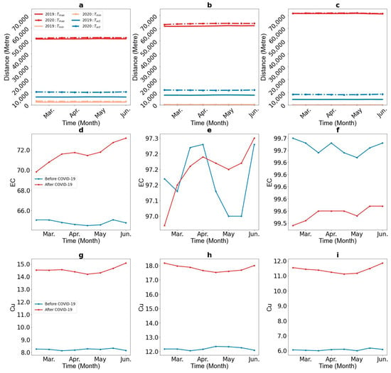
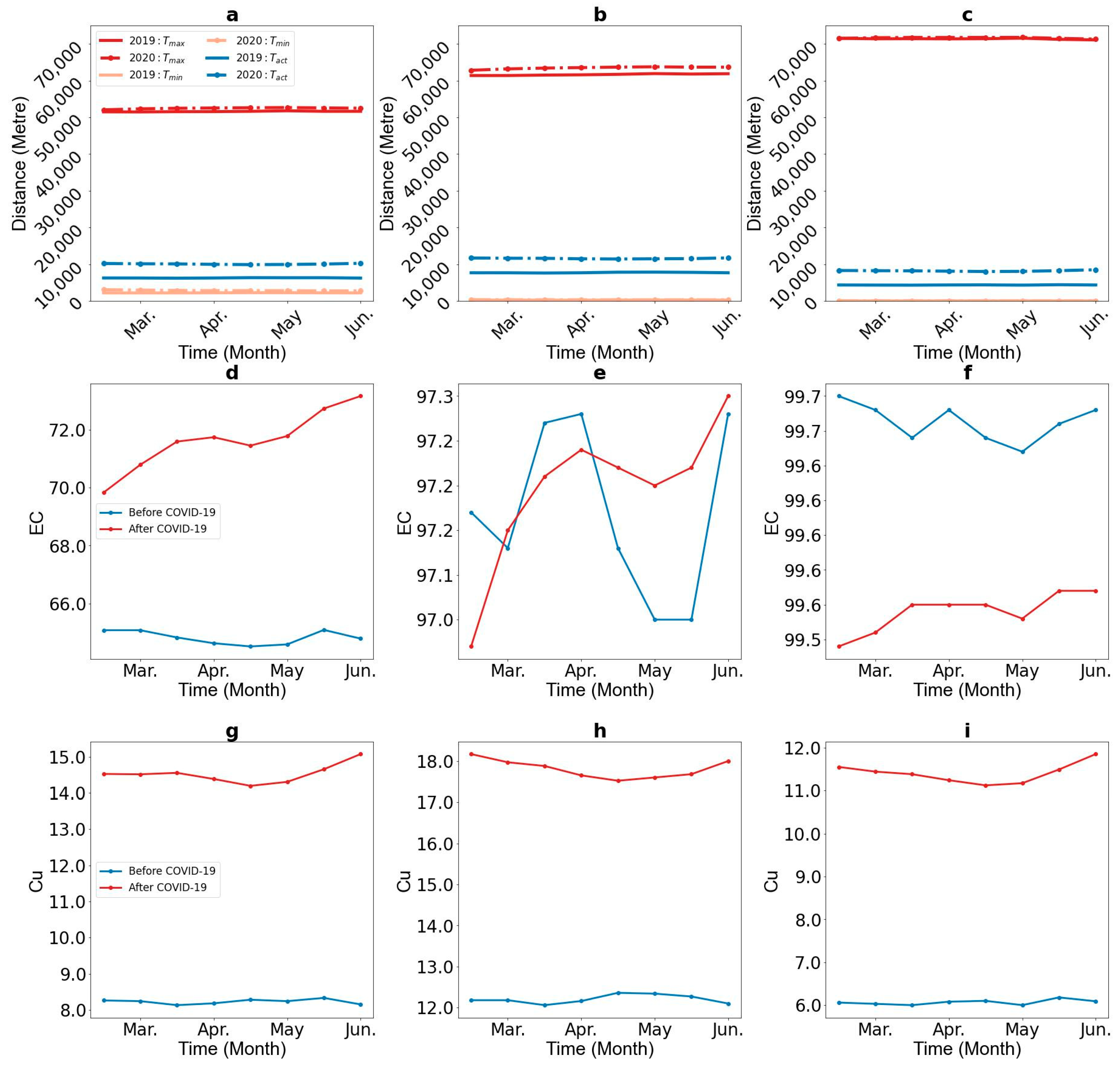
We used the excess commuting method with slack variables to calculate $T_{act}$, $T_{min}$ and $T_{max}$ both before and during the pandemic, as shown in Figure 6. These metrics allow us to better understand the jobs–housing relationships of various groups. The results from the full sample set show a notable increase in $T_{act}$ during the pandemic, rising from 6267 m to 10,058 m. $T_{act}$ for older adults (4342 m) and young people (7715 m) showed an increasing trend. However, after the pandemic began, $T_{act}$ for all groups leveled out to approximately 10,000 m. Regarding $T_{max}$, young individuals had a maximum theoretical commuting travel distance of around 60,000 m, while older adults had around 70,000 m. We found that $T_{min}$ remained under 500 m for various groups, as a smaller $T_{min}$ indicates that most people could find housing close to their workplaces, which conveys a meaning similar to that expressed by the jobs–housing ratio. The changes in both $T_{max}$ and $T_{min}$ were relatively minor.

Figure 6. Changes in commuting distance, excess commuting (EC), and commuting capacity utilization ($C_u$) before and during the COVID-19 pandemic. Graphs (a–c) represent the commuting distance of full sample set, the young adults sub-sample set, and the older adults sub-sample set, respectively. Graphs (d–f) represent the $EC$ of the full sample set, the young adults sub-sample set, and the older adults sub-sample set, respectively. Graphs (g–i) represent the commuting capacity utilization $C_u$ of the full sample set, the young adults sub-sample set, and the older adults sub-sample set, respectively.

Based on the aforementioned results, we further calculated $EC$ before and during the pandemic, as shown in Figure 6. It is evident that after the outbreak of the epidemic, excess commuting in Beijing significantly increased. This suggests that there was a rising trend in commuting distance after the outbreak of COVID-19. When comparing different demographic groups, it was observed that older adults exhibited a notable increase in excess commuting after the outbreak of COVID-19, while that of younger individuals did not display a significant change. The observed increase in commuting distance suggests that overall commuting efficiency in Beijing declined after the pandemic; viewed from the perspective of land use, this decline simultaneously reflects a weakening of urban land resource allocation efficiency, with heterogeneous impacts across demographic groups underscoring the unequal distribution of efficiency losses in the urban spatial structure.

The $EC$ of the sub-sample is calculated based on the assumption that the number of workplaces and residential locations is unequal. Therefore, with the work location being fixed, each sub-sample has more residential location choices compared to the original method, leading to a smaller $T_{\mathrm{m}\mathrm{i}\mathrm{n}}$ and a larger $T_{\mathrm{m}\mathrm{a}\mathrm{x}}$ compared to the full sample. As a result, the $EC$ for sub-samples is greater than the average of the full sample.

Figure 6 jointly plots the realized mean commute $T_{act}$ and its feasible bounds $T_{max}$ and $T_{min}$. Across the pre- and post-COVID-19 periods, $T_{min}$ and $T_{max}$ are broadly stable, implying that spatial opportunities did not materially deteriorate. Nevertheless, $T_{act}$ rise, indicating a widening behavioral gap between realized trips and the spatially attainable lower bound. At the same time, combining changes in trip frequency and trip distance shows that aggregate commuting decreases by 15.4% after the outbreak. In other words, the pandemic reduced how much people commuted overall, while those who continued to commute adopted routes/times that were less efficient relative to the feasible benchmark (e.g., transfer avoidance, off-peak shifts, and other substitutions). This joint pattern explains why EC can rise even when total mobility falls and is therefore consistent with the broader behavioral changes induced by COVID-19 rather than a change in the underlying jobs–housing opportunity set.

Unlike $EC$, $C_u$ are more stable, as the calculation process eliminates the impact of sample variation on excess commuting [12,43]. By comparing the $C_u$ of each sub-sample with that of the full sample, it is evident that the $C_u$ of the full sample lies between those of the sub-samples, which also reflects the comparability of $C_u$ across different samples. To facilitate a direct comparison of commuting demands across different groups and periods, we computed $C_u$, as depicted in Figure 6. We found that following the outbreak of COVID-19, the commuting distance of all groups showed a similar trend, namely, a decrease in urban commuting efficiency after the COVID-19 pandemic.

4.2. Spatial Causes of Excess Commuting Changes

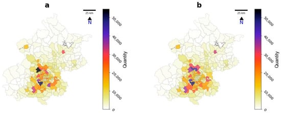
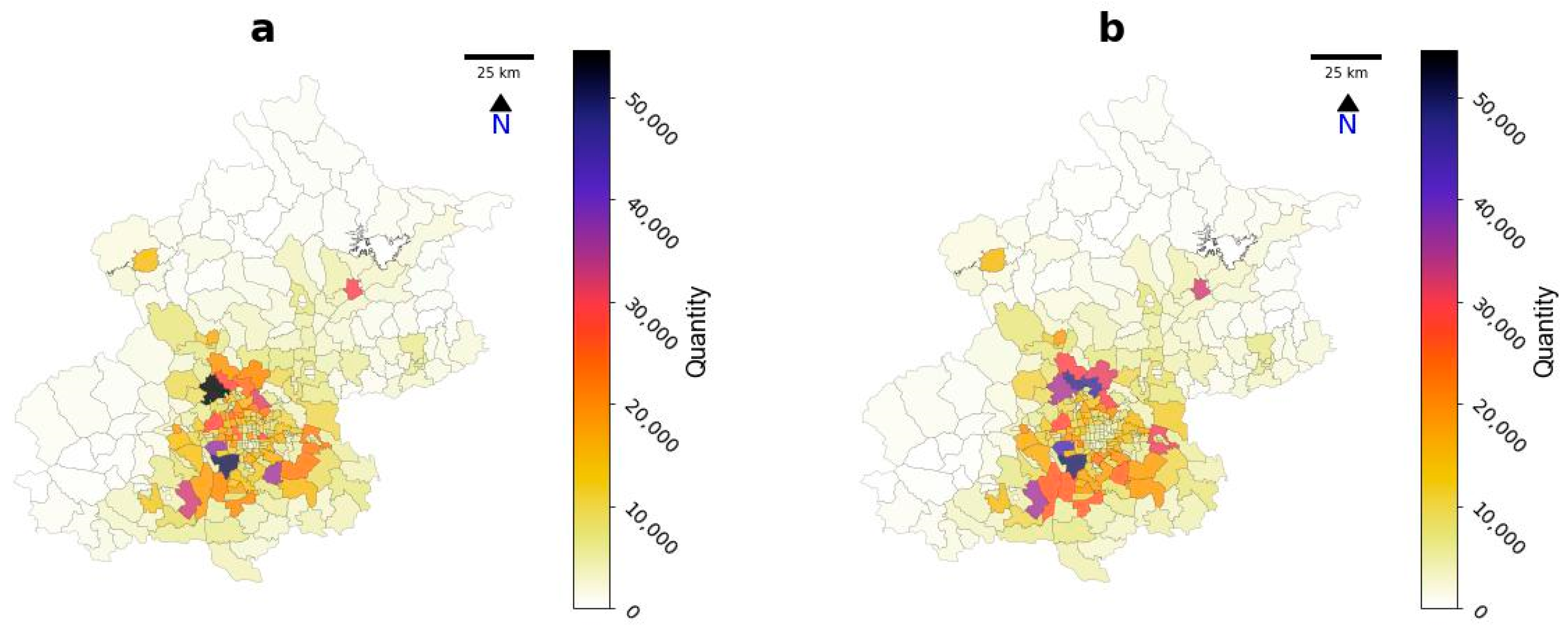
To investigate the causes of changes in excess commuting before and during the pandemic, we display the average number of residences and workplaces within each jiedao during the observation period, as illustrated in Figure 7. Based on the statistical analysis of the number of residences and workplaces in the central region, we find that a substantial amount of work is concentrated in the core area, and workplaces are more concentrated than residences. Workplaces in the central area constitute 58.5% of the city’s total workplaces, while residences account for 52.0%. By comparing the number of residences and workplaces in the core area before and during the COVID-19 pandemic, it is noticeable that there was no noticeable change in the number of workplaces (58.5% before the outbreak and 58.4% after), but there was a decline in the number of residences (from 52.6% before the epidemic to 51.4% after).

Figure 7. Spatial distribution of residential locations and workplaces. Graphs (a,b) are spatial distributions of jobs and the spatial distribution of housing for Beijing, respectively.

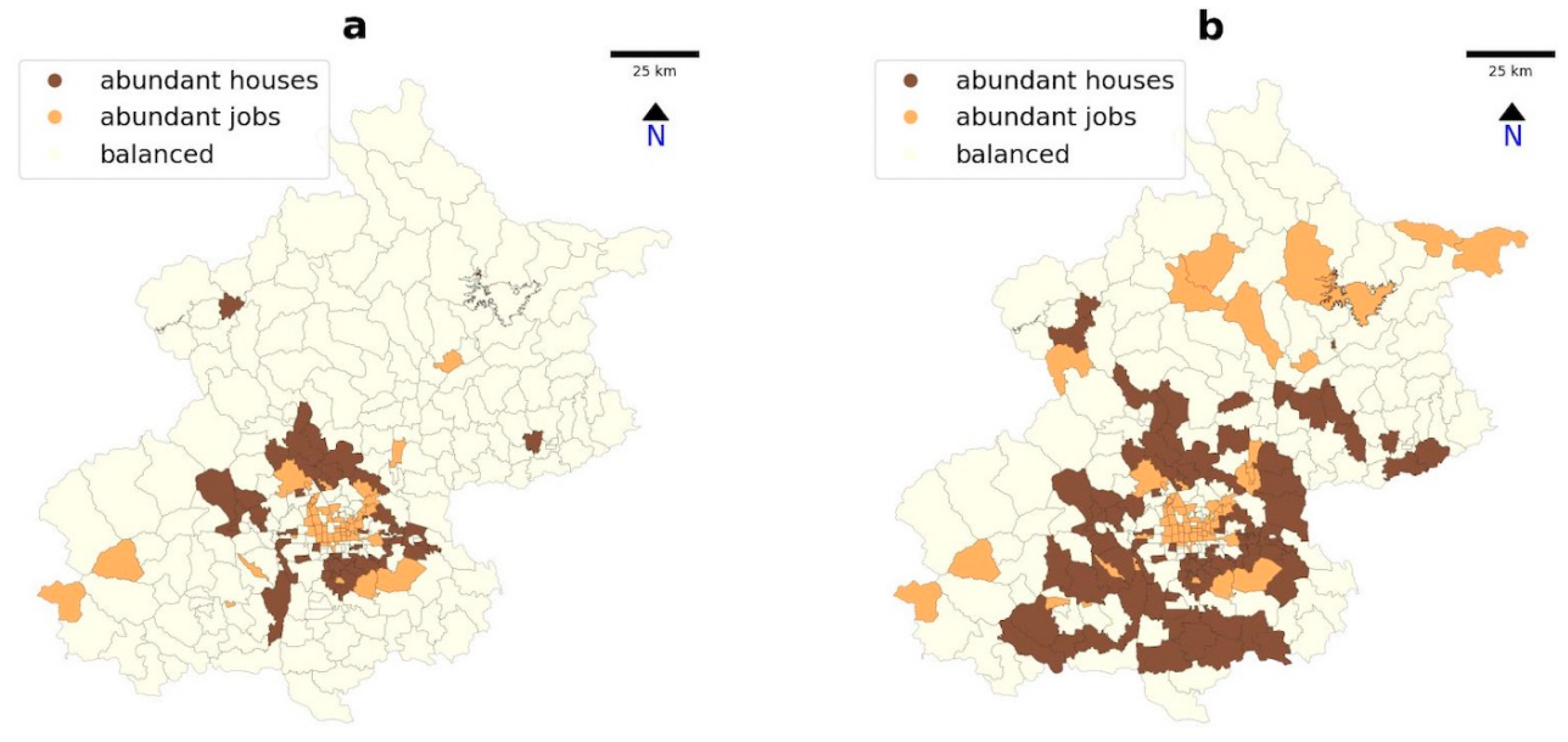
To gain a better understanding of whether there is a division of labor between workplaces and residential locations across jiedao, we calculated the JHR for different jiedaos, which can be used to analyze the abundance of residential locations and workplaces on these jiedaos, as shown in Figure 8. We find that there is a clear division among different jiedao. Namely, areas rich in workplaces are concentrated in the city center, while the peripheries of these employment-rich areas have a high concentration of residences. In contrast, suburbs exhibit a more balanced job–residence ratio. From the statistical analysis of JHR before and during the pandemic, we found that the average JHR rose following the outbreak, moving from 1.08 to 1.11. Concurrently, the standard deviation also experienced an increase, going from 0.54 to 0.70. By comparing the JHR of jiedao in the central area to those in the suburbs, we found that after the outbreak of COVID-19, the average JHR of jiedao in the central area decreased by 3%, while the average JHR of jiedao in the suburbs increased by 20%.

Figure 8. The impact of COVID-19 on JHR and SCE. Graphs (a,b) represent the JHR before and during the COVID-19 pandemic, respectively.

Compared to JHR, the SCE incorporates residents’ location choice. Therefore, we can analyze changes in commuting distance of different populations before and during the COVID-19 pandemic by comparing RSCE, as shown in Figure 8. We find that the proportion of areas with a relative increase in SCE for the young is smaller compared to older adults. In central areas of Beijing, for young people, 6% of central area neighborhoods and 7% of non-central area neighborhoods show a relative increase in SCE.

4.3. Differences in Excess Commuting Among Groups with Different Characteristics

In the wake of the COVID-19 outbreak, residence–workplace choices changed across different ages. To determine which groups adjusted more, we implement a DID design to estimate the pandemic’s impact on commuting distances by group. For comparisons among different age groups, young people were selected as the control group. In the model, the dependent variable is $C_u$, which can eliminate the bias of sample variation. Due to the presence of a time budget, we select non-commuting speed, non-commuting frequency, commuting speed, and commuting frequency as control variables [52]. Due to the difficulty in accurately calculating travel speeds using Call Detail Record (CDR) data, we have corrected the travel speeds in the mobile signaling data using data from the Beijing Transport Development Annual Report. The statistical description of the control variables used in this paper is shown in Table 2, which reports the means and standard deviations (in parentheses) for each group.

Table 2. Descriptive statistics of control variables used in the difference-in-differences model.

	Young Adults	Older Adults	Total
Commuting frequency	26.99 (13.34)	27.65 (15.12)	27.24 (14.05)
Non-Commuting frequency	58.0 (35.44)	62.15 (37.1)	59.71 (36.19)
Commuting speed (Km/Hour)	17.13 (42.98)	18.23 (43.47)	17.55 (43.17)
Non-Commuting speed (Km/Hour)	27.81 (32.67)	27.94 (32.6)	27.86 (32.64)

Note: The control variables include four indicators related to travel behavior, selected to address the impact of time budget constraints on commuting efficiency. The main values in the table represent the mean of each control variable for different groups, reflecting the central tendency of the data. The values in parentheses represent the standard deviation, reflecting the degree of dispersion of the data around the mean.

The parallel trends assumption is essential for DID analysis. To ensure the reliability of our results, (a) we start with the ADF (Augmented Dickey–Fuller) test. Applying an Augmented Dickey–Fuller test to the pre-period treated–control difference directly targets this property: rejecting a unit root indicates the difference is stationary rather than a random walk with drift. Stationarity of the pre-period gap is therefore consistent with—indeed, a necessary condition for—parallel trends, because a nonstationary, drifting gap would violate the assumption. If the difference in $C_u$ between the treatment group and the control group is stable, it indicates they follow similar trends. The ADF (Augmented Dickey–Fuller) test results, showing t-values of −5.02 for age, indicate that the differences in $C_u$ between sub-samples for these categories are statistically significant. Next, (b) we include time fixed effects before the pandemic outbreak in our analysis [53]. Estimating pre-pandemic regressions with month indicators asks whether there are systematic month-to-month deviations in the treated–control gap prior to the shock. If the month effects (net of group means) are jointly insignificant, the gap does not vary systematically across months, which is exactly what parallel trends require in the pre-period: no structured temporal divergence between the groups before treatment. In other words, the month dummies test rules out deterministic pre-trend patterns (e.g., seasonal or stepwise differences), complementing the ADF test that rules out stochastic drift. If these effects are found to be insignificant, it suggests that there were no notable differences between the treatment group and the control group. Table 3 shows that $C_u$ has met the criteria for the parallel trends test before the pandemic outbreak. (c) As illustrated in Figure 6h,i, Cu traces a broadly similar trajectory across the pre- and post-COVID-19 periods: month-to-month movements are aligned, and the slopes on either side of the outbreak are comparable. This visual pattern suggests no pronounced structural break around the onset and is consistent with the parallel-trends premise underlying our DID analysis.

Table 3. DID regression results for testing the parallel trends assumption.

Month (Older Adults vs. Young Adults)	Coefficient
March 2019	−0.0278 (−1.1389)
April 2019	−0.0281 (−1.1512)
May 2019	−0.0288 (−1.1807)
June 2019	−0.028 (−1.1467)
July 2019	−0.0269 (−1.1017)
August 2019	−0.0278 (−1.1377)
September 2019	−0.0273 (−1.1159)
October 2019	−0.0289 (−1.183)
Control Group	0.0217 *** (2.5829)
Intercept	0.1032 *** (16.3663)

Note: This table reports the coefficients for testing the parallel trends assumption. The dependent variable is the difference in Commuting Capacity Utilization ($C_u$) between the older adult and young adult groups. Values in parentheses are t-statistics. The statistically insignificant coefficients for all pre-treatment months indicate that the parallel trends assumption holds. ***, **, and * indicate statistical significance at the 1%, 5%, and 10% levels, respectively.

The regression results shown in Table 4 indicate that the interaction terms are significantly negative. These findings demonstrate that, in comparison to younger residents, older adults show a significant increase in commuting distance following the outbreak of COVID-19. Including control variables in the analysis does not significantly change the interaction term, suggesting that our results are robust. Additionally, we observe that commuting speed is significantly and negatively correlated with $C_u$, meaning that an increase in commuting speed leads to a significant rise in commuting distance. Conversely, non-commuting speed is significantly and positively associated with $C_u$, indicating that an increase in non-commuting speed results in a significant decrease in commuting distance. We also found that non-commuting travel frequency is negatively correlated with $C_u$, meaning that an increase in non-commuting travel demand will also lead to an increase in commuting distance.

Table 4. DID regression results for age-heterogeneous changes in commuting efficiency.

Variable	Model (1) and Model (2) with Controls
COVID-19	5.6311 *** (47.8183)	5.2326 *** (32.1465)
Group	−6.1111 *** (−51.8944)	−6.1037 *** (−63.0328)
Group × COVID-19	−0.2924 * (−1.7559)	−0.2991 ** (−2.1841)
Non-Commuting Speed		0.037 *** (2.8328)
Commuting Speed		−0.059 *** (−3.1755)
Non-Commuting Frequency		−0.0339 *** (−3.0493)
Commuting Frequency		−0.0257 (−0.8803)
Intercept	12.1776 *** (146.2439)	15.5248 *** (12.4293)
$R^2$	0.9602	0.9714
Observations	32	32

Note: The dependent variable is Commuting Capacity Utilization ($C_u$). Values are regression coefficients with t-statistics in parentheses. The key variable of interest is the interaction term (Group × COVID-19). ***, **, and * indicate statistical significance at the 1%, 5%, and 10% levels, respectively.

To assess robustness, we re-estimate the models under alternative sample windows. As reported in Table 5, the treatment-by-post interaction remains statistically significant across all windows and varies only modestly in magnitude, supporting the robustness of our conclusions.

Table 5. Window sensitivity checks.

	March–July		March–August		March–September
COVID-19	5.6206 *** (40.3897)	5.3139 *** (32.2431)	5.5045 *** (46.658)	5.2786 *** (44.3231)	5.6311 *** (47.8183)	5.2326 *** (32.1465)
Group	−6.1336 *** (−44.0767)	−6.1184 *** (−64.2661)	−6.1187 *** (−51.8646)	−6.1312 *** (−84.952)	−6.1111 *** (−51.8944)	−6.1037 *** (−63.0328)
Group × COVID-19	−0.3477 * (−1.7666)	−0.3643 ** (−2.7061)	−0.1839 (−1.1021)	−0.3487 *** (−3.4166)	−0.2924 * (−1.7559)	−0.2991 ** (−2.1841)
Non-Commuting Speed		0.023 (1.3052)		0.0102 (0.7438)		0.037 *** (2.8328)
Commuting Speed		−0.0386 (−1.535)		−0.0134 (−0.7201)		−0.059 *** (−3.1755)
Non-Commuting Frequency		−0.0222 * (−2.0719)		−0.0143 * (−1.7484)		−0.0339 *** (−3.0493)
Commuting Frequency		0.0027 (0.0628)		0.0327 (0.9939)		−0.0257 (−0.8803)
Intercept	12.1776 *** (123.7568)	14.0055 *** (8.7269)	12.1777 *** (145.9796)	12.1714 *** (10.6703)	12.1776 *** (146.2439)	15.5248 *** (12.4293)
${\mathit{R}}^2$	0.9634	0.9771	0.9649	0.9759	0.9602	0.9714
Observations	20	20	24	24	28	28

Note: ***, **, and * indicate statistical significance at the 1%, 5%, and 10% levels, respectively.

5. Discussion

Our findings support the proposed mechanism through which an external shock reduces urban land resource allocation efficiency via exacerbating the jobs–housing mismatch. The COVID-19 pandemic, as a quintessential exogenous shock, triggered two key behavioral responses that disrupted the spatial equilibrium: (1) an increase in remote work, which decouples the physical workplace from the residence and reduces the weight of commuting cost in residential location choice [54]; and (2) a preference for relocating to areas perceived as having lower infection risks [55]. Critically, these behaviors did not symmetrically affect job locations, which remain clustered in city centers due to agglomeration economies and higher relocation costs for firms [56]. This asymmetric adjustment—where residences decentralize more readily than jobs—strengthened the center-periphery spatial pattern (as shown by our JHR results) and directly led to the observed surge in excess commuting. This spatial restructuring is empirically validated by our JHR results, which show a rising city-wide ratio (1.08 to 1.11) and a sharp 20% increase in suburban JHR, confirming the intensified jobs–housing separation at the metropolitan scale. The lengthening of commutes, as captured by our EC and $C_u$ metrics, represents a tangible efficiency loss: more land is dedicated to transportation infrastructure, more time is spent unproductively in transit, and energy consumption and emissions rise. Therefore, the increase in excess commuting is not merely a transportation issue but a direct indicator of worsened spatial resource allocation efficiency under external shocks.

The heterogeneous impact on older adults, as identified by our DID model, further elucidates this ‘asymmetric adjustment’ mechanism. We hypothesize that the older adult population is not monolithic in their response to the shock. While a segment might have had the option to work remotely [56], a significant portion, likely in roles that require physical presence, did not. It is this latter group that drove the observed result. Our RSCE findings suggest that older adults, potentially being more risk-averse, exhibited a stronger preference for relocating to peripheral areas [52]. However, their job locations, often in centralized sectors less amenable to remote work, remained fixed [57]. For those unable to telecommute, this resulted in a drastic increase in commuting distances. This heightened asymmetry explains their more severe efficiency loss. Furthermore, this asymmetry was likely compounded by occupation- and mode-specific factors: older workers’ lower access to teleworkable jobs and a potential shift away from public transit may have jointly led to longer, less efficient commutes [52,57]. In contrast, younger adults, possibly due to greater job mobility or different risk perceptions, exhibited a less pronounced residential decentralization relative to their job locations, leading to a smaller increase in excess commuting.

When situated within the broader literature, our findings both confirm and extend existing knowledge. The overall increase in excess commuting aligns with the post-COVID-19 pattern documented by [15]. However, our study reveals that the classical framework of [11,12], which assumes balanced jobs–housing totals, would underestimate the inefficiency for demographic subgroups. By introducing a generalized model with slack variables, we not only provide a more realistic city-level measure but also unlock the capability to conduct heterogeneity analysis—a critical advancement for understanding equitable urban development. Furthermore, while prior research has noted the stability of employment centers [57], our results quantify how behavioral shocks can exacerbate the spatial mismatch with decentralized residences, leading to measurable efficiency losses that were previously more difficult to attribute.

Improvements in transport infrastructure do not necessarily lead to a decrease in excess commuting. This is because, while commuting is mandatory travel, minimizing commuting is not the only goal residents consider when deciding where to live and work [57]. When the workplace location is fixed, the choice of residence is also influenced by the attractiveness of the location and individual preferences. This means that in the process of residential location choice, residents try to seek a balance between commuting travel and non-commuting travel. For instance, in some residential location choice models, it is assumed that people might be willing to accept a longer commute in order to benefit from more convenient non-commuting travel [58,59].

6. Conclusions

Theoretically, this study contributes by introducing a more general framework for assessing excess commuting that accommodates imbalances between jobs and residences. The approach yields system-wide measures of excess commuting and, crucially, permits heterogeneity analysis—it can identify and compare excess-commuting differentials across demographic or behavioral subgroups. This enables an evaluation of urban land use efficiency from the perspective of spatial allocation efficiency.

Our empirical findings further reinforce these contributions and offer salient policy implications: after the COVID-19 outbreak, Beijing’s urban commuting efficiency declined significantly, with the observed average commuting distance ($T_{act}$) of residents increasing by 59% (from 6267 m to 10,058 m), which directly reflects a reduction in urban land resource allocation efficiency. Spatially, a more pronounced center-periphery structure emerged: the average jobs–housing ratio (JHR) rose from 1.08 to 1.11 (standard deviation: 0.54 → 0.70), with the JHR of central urban areas decreasing by 3% and suburban areas increasing by 20%—confirming intensified jobs–housing separation. Heterogeneity analysis via DID regression (Group × COVID-19 = −0.2991 **, p < 0.05) showed that older adults suffered disproportionately greater commuting inefficiency than younger adults when taking young adults as the control group. Thus, in designing post-pandemic recovery strategies, policymakers should develop differentiated interventions for older adults. For those capable of remote work, enhancing digital infrastructure is key. For those in non-telecommutable jobs, policies should focus on optimizing the housing–employment balance in their residential areas and improving public transit accessibility.

However, this study has the following limitations: (a) The research only uses data from one year before and one year after the pandemic to analyze the impact of COVID-19 on residential and employment demand, without verifying the long-term effects of the pandemic. (b) While commuting is an individual behavior, this study uses jiedao-level (sub-district-level) data to analyze the distribution and demand of residences and employment. Although this is a standard and practical approach, the variation in jiedao size and population might introduce some aggregation bias. Future research could benefit from exploring the sensitivity of results using different spatial units or finer-grained data. (c) Our demographic categorization is constrained by data availability. While the age-based grouping is theoretically grounded, the observed effect may correlate with unobserved socio-economic factors such as occupation and income.

References

- Perera, C.; Zaslavsky, A.; Christen, P.; Georgakopoulos, D. Sensing as a service model for smart cities supported by internet of things. Trans. Emerg. Telecommun. Technol. 2014, 25, 81–93. [Google Scholar] [CrossRef] [Scilit]
- Zhang, X.Q. The trends, promises and challenges of urbanisation in the world. Habitat Int. 2016, 54, 241–252. [Google Scholar] [CrossRef] [Scilit]
- Han, F.; Xie, R.; Lai, M. Traffic density, congestion externalities, and urbanization in China. Spat. Econ. Anal. 2018, 13, 400–421. [Google Scholar] [CrossRef] [Scilit]
- Mishra, A.K. Cities, transport and agglomeration: Addressing the urban mobility challenges in India. Growth Change 2019, 50, 1115–1133. [Google Scholar] [CrossRef] [Scilit]
- Sun, H.; Pofoura, A.K.; Mensah, I.A.; Li, L.; Mohsin, M. The role of environmental entrepreneurship for sustainable development: Evidence from 35 countries in Sub-Saharan Africa. Sci. Total Environ. 2020, 741, 140132. [Google Scholar] [CrossRef] [Scilit]
- Giuliano, G. Is jobs-housing balance a transportation issue? Transp. Res. Rec. 1991, 1305, 305–312. [Google Scholar]
- Yan, S.; Peng, J.; Wu, Q. Exploring the non-linear effects of city size on urban industrial land use efficiency: A spatial econometric analysis of cities in eastern China. Land Use Policy 2020, 99, 104944. [Google Scholar] [CrossRef] [Scilit]
- Zheng, Z.; Zhou, S.; Deng, X. Exploring both home-based and work-based jobs-housing balance by distance decay effect. J. Transp. Geogr. 2021, 93, 103043. [Google Scholar] [CrossRef] [Scilit]
- Wang, H.; Zeng, W.; Cao, R. Simulation of the urban jobs–housing location selection and spatial relationship using a multi-agent approach. ISPRS Int. J. Geo-Inf. 2021, 10, 16. [Google Scholar] [CrossRef] [Scilit]
- Xiao, W.; Li, H.; Wei, Y.D. Understanding jobs-housing imbalance in urban China. J. Transp. Land Use 2021, 14, 389–415. [Google Scholar] [CrossRef] [Scilit]
- White, M.J. Location choice and commuting behavior in cities with decentralized employment. J. Urban Econ. 1988, 24, 129–152. [Google Scholar] [CrossRef] [Scilit]
- Horner, M.W.; Murray, A.T. Excess commuting and the modifiable areal unit problem. Urban Stud. 2002, 39, 131–139. [Google Scholar] [CrossRef] [Scilit]
- Suzuki, T.; Lee, S. Jobs–housing imbalance, spatial correlation, and excess commuting. Transp. Res. Part A Policy Pract. 2012, 46, 322–336. [Google Scholar] [CrossRef] [Scilit]
- Schleith, D.; Widener, M.; Kim, C. An examination of the jobs-housing balance of different categories of workers across 26 metropolitan regions. J. Transp. Geogr. 2016, 57, 145–160. [Google Scholar] [CrossRef] [Scilit]
- Chen, R.; Zhang, M.; Zhou, J. Jobs-housing relationships before and amid COVID-19: An excess-commuting approach. J. Transp. Geogr. 2023, 106, 103507. [Google Scholar] [CrossRef] [Scilit]
- Winters, M.; Sims-Gould, J.; Franke, T.; McKay, H. “I grew up on a bike”: Cycling and older adults. J. Transp. Health 2015, 2, 58–67. [Google Scholar] [CrossRef] [Scilit]
- Van Cauwenberg, J.; de Geus, B.; Deforche, B. Cycling for transport among older adults: Health benefits, prevalence, determinants, injuries and the potential of E-bikes. In Geographies of Transport Ageing; Palgrave Macmillan: Cham, Switzerland, 2018; pp. 133–151. [Google Scholar]
- Jang, W.M.; Kim, U.-N.; Jang, D.H.; Jung, H.; Cho, S.; Eun, S.J.; Lee, J.Y. Influence of trust on two different risk perceptions as an affective and cognitive dimension during Middle East respiratory syndrome coronavirus (MERS-CoV) outbreak in South Korea: Serial cross-sectional surveys. BMJ Open 2020, 10, e033026. [Google Scholar] [CrossRef] [Scilit]
- Callen, M.; Isaqzadeh, M.; Long, J.D.; Sprenger, C. Violence and risk preference: Experimental evidence from Afghanistan. Am. Econ. Rev. 2014, 104, 123–148. [Google Scholar] [CrossRef] [Scilit]
- Huang, L.; Zhou, Y.; Han, Y.; Hammitt, J.K.; Bi, J.; Liu, Y. Effect of the Fukushima nuclear accident on the risk perception of residents near a nuclear power plant in China. Proc. Natl. Acad. Sci. USA 2013, 110, 19742–19747. [Google Scholar] [CrossRef] [Scilit]
- Ibuka, Y.; Chapman, G.B.; Meyers, L.A.; Li, M.; Galvani, A.P. The dynamics of risk perceptions and precautionary behavior in response to 2009 (H1N1) pandemic influenza. BMC Infect. Dis. 2010, 10, 296. [Google Scholar] [CrossRef] [Scilit]
- Klaiber, P.; Wen, J.H.; DeLongis, A.; Sin, N.L. The ups and downs of daily life during COVID-19: Age differences in affect, stress, and positive events. J. Gerontol. Ser. B 2021, 76, e30–e37. [Google Scholar] [CrossRef] [Scilit] [PubMed]
- Alsharawy, A.; Spoon, R.; Smith, A.; Ball, S. Gender differences in fear and risk perception during the COVID-19 pandemic. Front. Psychol. 2021, 12, 689467. [Google Scholar] [CrossRef] [Scilit] [PubMed]
- Mroczek, D.K.; Almeida, D.M. The effect of daily stress, personality, and age on daily negative affect. J. Personal. 2004, 72, 355–378. [Google Scholar] [CrossRef] [Scilit] [PubMed]
- Wrzus, C.; Müller, V.; Wagner, G.G.; Lindenberger, U.; Riediger, M. Affective and cardiovascular responding to unpleasant events from adolescence to old age: Complexity of events matters. Dev. Psychol. 2013, 49, 384. [Google Scholar] [CrossRef] [Scilit]
- Tricarico, L.; De Vidovich, L. Proximity and post-COVID-19 urban development: Reflections from Milan, Italy. J. Urban Manag. 2021, 10, 302–310. [Google Scholar] [CrossRef] [Scilit]
- Jo, Y.; Hong, A.; Sung, H. Density or connectivity: What are the main causes of the spatial proliferation of COVID-19 in Korea? Int. J. Environ. Res. Public Health 2021, 18, 5084. [Google Scholar] [CrossRef] [Scilit]
- Peng, Z.-R. The jobs-housing balance and urban commuting. Urban Stud. 1997, 34, 1215–1235. [Google Scholar] [CrossRef] [Scilit]
- Cervero, R. Jobs-housing balancing and regional mobility. J. Am. Plan. Assoc. 1989, 55, 136–150. [Google Scholar] [CrossRef] [Scilit]
- Glaeser, E.L.; Kahn, M.E.; Rappaport, J. Why do the poor live in cities? The role of public transportation. J. Urban Econ. 2008, 63, 1–24. [Google Scholar] [CrossRef] [Scilit]
- Evans, G.W.; Wener, R.E.; Phillips, D. The morning rush hour: Predictability and commuter stress. Environ. Behav. 2002, 34, 521–530. [Google Scholar] [CrossRef] [Scilit]
- Gottholmseder, G.; Nowotny, K.; Pruckner, G.J.; Theurl, E. Stress perception and commuting. Health Econ. 2009, 18, 559–576. [Google Scholar] [CrossRef] [Scilit] [PubMed]
- Giuliano, G.; Small, K.A. Is the journey to work explained by urban structure? Urban Stud. 1993, 30, 1485–1500. [Google Scholar] [CrossRef] [Scilit]
- Saadi, I.; Boussauw, K.; Teller, J.; Cools, M. Trends in regional jobs-housing proximity based on the minimum commute: The case of Belgium. J. Transp. Geogr. 2016, 57, 171–183. [Google Scholar] [CrossRef] [Scilit]
- Gordon, P.; Richardson, H.W. Are compact cities a desirable planning goal? J. Am. Plan. Assoc. 1997, 63, 95–106. [Google Scholar] [CrossRef] [Scilit]
- Scheiner, J.; Holz-Rau, C. A comprehensive study of life course, cohort, and period effects on changes in travel mode use. Transp. Res. Part A Policy Pract. 2013, 47, 167–181. [Google Scholar] [CrossRef] [Scilit]
- Nurdden, A.; Rahmat, R.; Ismail, A. Effect of transportation policies on modal shift from private car to public transport in Malaysia. J. Appl. Sci. 2007, 7, 1013–1018. [Google Scholar] [CrossRef] [Scilit]
- Chang, Y.-C. Factors affecting airport access mode choice for elderly air passengers. Transp. Res. Part E Logist. Transp. Rev. 2013, 57, 105–112. [Google Scholar] [CrossRef] [Scilit]
- Hamilton, B.W.; Röell, A. Wasteful commuting. J. Political Econ. 1982, 90, 1035–1053. [Google Scholar] [CrossRef] [Scilit]
- Niedzielski, M.A.; Horner, M.W.; Xiao, N. Analyzing scale independence in jobs-housing and commute efficiency metrics. Transp. Res. Part A Policy Pract. 2013, 58, 129–143. [Google Scholar] [CrossRef] [Scilit]
- Bwire, H.; Zengo, E. Comparison of efficiency between public and private transport modes using excess commuting: An experience in Dar es Salaam. J. Transp. Geogr. 2020, 82, 102616. [Google Scholar] [CrossRef] [Scilit]
- Murphy, E. Excess commuting and modal choice. Transp. Res. Part A Policy Pract. 2009, 43, 735–743. [Google Scholar] [CrossRef] [Scilit]
- Horner, M.W. Extensions to the concept of excess commuting. Environ. Plan. A Econ. Space 2002, 34, 543–566. [Google Scholar] [CrossRef] [Scilit]
- Ma, K.-R.; Banister, D. Extended excess commuting: A measure of the jobs-housing imbalance in Seoul. Urban Stud. 2006, 43, 2099–2113. [Google Scholar] [CrossRef] [Scilit]
- Murphy, E.; Killen, J.E. Commuting economy: An alternative approach for assessing regional commuting efficiency. Urban Stud. 2011, 48, 1255–1272. [Google Scholar] [CrossRef] [Scilit]
- Huang, J.; Hu, Y.; Wang, J.; Li, X. A tale of two cities: Jobs–housing balance and urban spatial structures from the perspective of transit commuters. Environ. Plan. B Urban Anal. City Sci. 2021, 48, 1543–1557. [Google Scholar] [CrossRef] [Scilit]
- Ewing, R.; Dumbaugh, E.; Brown, M. Internalizing travel by mixing land uses: Study of master-planned communities in South Florida. Transp. Res. Rec. 2001, 1780, 115–128. [Google Scholar] [CrossRef] [Scilit]
- Wu, J.; He, Q.; Chen, Y.; Lin, J.; Wang, S. Dismantling the fence for social justice? Evidence based on the inequity of urban green space accessibility in the central urban area of Beijing. Environ. Plan. B Urban Anal. City Sci. 2020, 47, 626–644. [Google Scholar] [CrossRef] [Scilit]
- Li, Z.; Hu, D. Exploring the relationship between the 2D/3D architectural morphology and urban land surface temperature based on a boosted regression tree: A case study of Beijing, China. Sustain. Cities Soc. 2022, 78, 103392. [Google Scholar] [CrossRef] [Scilit]
- Zheng, Z.; Zhou, W.; Wang, J.; Hu, X.; Qian, Y. Sixty-year changes in residential landscapes in Beijing: A perspective from both the horizontal (2D) and vertical (3D) dimensions. Remote Sens. 2017, 9, 992. [Google Scholar] [CrossRef] [Scilit]
- Shemer, L.; Shayanfar, E.; Avner, J.; Miquel, R.; Mishra, S.; Radovic, M. COVID-19 impacts on mobility and travel demand. Case Stud. Transp. Policy 2022, 10, 2519–2529. [Google Scholar] [CrossRef] [Scilit]
- Cui, Y.; Zhao, P.; Li, L.; Li, J.; Gong, M.; Deng, Y.; Si, Z.; Yan, S.; Dang, X. A new model for residential location choice using residential trajectory data. Humanit. Soc. Sci. Commun. 2024, 11, 255. [Google Scholar] [CrossRef] [Scilit]
- Deng, Y.; Zhao, P. The impact of new metro on travel behavior: Panel analysis using mobile phone data. Transp. Res. Part A Policy Pract. 2022, 162, 46–57. [Google Scholar] [CrossRef] [Scilit]
- Li, Z.; Zhao, P.; Yu, L.; Hai, X.; Feng, Y. The changes in job-housing balance during the COVID-19 period in China. Cities 2023, 137, 104313. [Google Scholar] [CrossRef] [Scilit] [PubMed]
- Obeid, H.; Anderson, M.L.; Bouzaghrane, M.A.; Walker, J. Does telecommuting reduce trip-making? Evidence from a US panel during the COVID-19 pandemic. Transp. Res. Part A Policy Pract. 2024, 180, 103972. [Google Scholar] [CrossRef] [Scilit]
- Ellison, G.; Glaeser, E.L.; Kerr, W.R. What causes industry agglomeration? Evidence from coagglomeration patterns. Am. Econ. Rev. 2010, 100, 1195–1213. [Google Scholar] [CrossRef] [Scilit]
- Loa, P.; Hossain, S.; Mashrur, S.M.; Liu, Y.; Wang, K.; Ong, F.; Habib, K.N. Exploring the impacts of the COVID-19 pandemic on modality profiles for non-mandatory trips in the Greater Toronto Area. Transp. Policy 2021, 110, 71–85. [Google Scholar] [CrossRef] [Scilit]
- Næss, P.; Strand, A.; Wolday, F.; Stefansdottir, H. Residential location, commuting and non-work travel in two urban areas of different size and with different center structures. Prog. Plan. 2019, 128, 1–36. [Google Scholar] [CrossRef] [Scilit]
- Wang, Y.; de Almeida Correia, G.H.; van Arem, B.; Timmermans, H.H. Understanding travellers’ preferences for different types of trip destination based on mobile internet usage data. Transp. Res. Part C Emerg. Technol. 2018, 90, 247–259. [Google Scholar] [CrossRef] [Scilit]
Disclaimer/Publisher’s Note: The statements, opinions and data contained in all publications are solely those of the individual author(s) and contributor(s) and not of MDPI and/or the editor(s). MDPI and/or the editor(s) disclaim responsibility for any injury to people or property resulting from any ideas, methods, instructions or products referred to in the content. |
© 2026 by the authors. Licensee MDPI, Basel, Switzerland. This article is an open access article distributed under the terms and conditions of the Creative Commons Attribution (CC BY) license.