


Abstract
Large, shallow lakes lacking rooted aquatic vegetation are susceptible to wind-induced wave action that results in increased shear stress on the lake bottom, sediment resuspension and poor water clarity. The relationship between meteorological, hydrographical and sediment characteristics, and sediment dynamics has implications for internal phosphorus cycling and bioavailability, the frequency and duration of harmful cyanobacterial blooms, lake level management and restoration potential. In this study, a multi-parameter water quality sonde was deployed at various sites at the bottom of Utah Lake to measure water quality variables. Sediment cores were collected at each of the deployment sites and analyzed for common physical and chemical properties. Several machine learning regression techniques, including polynomial, decision tree, artificial neural network, and support vector machine, were applied to predict turbidity, a measure of water clarity and surrogate for sediment dynamics, using the observed explanatory variables wind speed and direction, fetch, water depth, sediment properties, algae, and cyanobacteria. The decision tree estimators, random forest and histogram-based gradient boosting had the best model performance, explaining 86–89% of the variability in turbidity when including all the explanatory variables. The artificial neural network estimator multi-layer perceptron and the polynomial regression models also performed well (81%), whereas the support vector machine estimator exhibited poor performance. Chlorophyll and phycocyanin, components of turbidity, were amongst the most important variables to the decision tree and artificial neural network models. Wind speed and water depth were also of high importance, which conforms with mechanistic explanations of sediment mobility caused by wave action and shear stress. Carbonate content was consistently a good predictor due to the calcareous nature of Utah Lake, whereas the importance of the other sediment properties was dependent on the machine learning technique applied. This case study demonstrated the potential for machine learning models to predict water clarity and has promise for more general applications to other shallow lakes and serves as a useful tool for lake management and restoration.
1. Introduction
Shallow lakes (generally 5 m mean depth or less where sunlight reaches the lake bottom), particularly those with surface areas greater than 100 km2 and lacking submerged aquatic vegetation, have been found to be susceptible to turbulent mixing and sediment resuspension associated with elevated winds [1,2,3,4], resulting in negative biogeochemical consequences including poor water clarity and nutrient enrichment [5,6,7,8]. Eutrophication and low water transparency in turn impact light availability and primary productivity in the water column and benthos [9,10], which can lead to enhanced frequency and duration of harmful cyanobacterial blooms [11,12,13].
Wind blowing over lakes causes stress on the water surface that generates both water current velocities and waves. Horizontal water velocity is a function of wind velocity, wind duration, fetch (the length of open water over which wind travels) and water depth [1,14]. Resuspension of sediments in shallow lakes results from both wind-generated currents and wave action on the lake bottom [15,16,17]. The amount of sediment that becomes resuspended during wind events depends on wind velocity and duration, effective lake fetch, water depth, the presence and density of rooted aquatic vegetation and sediment characteristics [18,19,20,21,22].
The dependence of sediment resuspension on the complex interaction between wind speed and direction, lake hydrography, and sediment properties makes quantifying the dominant mechanisms and predicting turbidity challenging. Machine learning (ML) statistical techniques are well-suited to correlating high-frequency environmental monitoring data sets with multiple variables and require far less computational resources than process-based mechanistic modeling approaches [23,24,25]. Machine learning algorithms build models using sample data to make inferences or predictions without following explicit instructions [24]. Examples of ML algorithms include random forest regression tree, gradient boosting regression, support vector machines, and artificial neural networks [26].
Several studies have successfully applied machine learning approaches to predict sediment transport and load in advective riverine systems, including artificial neural network (ANN) modeling [27,28], support vector machine (SVM) regression [29], and Gaussian process regression [30]. More recent efforts have focused on the optimization of the machine learning model parameters to predict sediment load [31,32]. The application of machine learning models to evaluate and predict sediment resuspension and turbidity in shallow lakes is novel and has only recently been attempted in Lake Taihu [33,34].
This case study applies machine learning statistical regression techniques utilizing meteorological, hydrodynamic, water quality and sediment characteristic data collected from Utah Lake, a large, shallow, calcareous freshwater system located in a semi-arid setting, with the objective to construct a robust predictive turbidity model that captures the spatial and temporal heterogeneity of the lake using minimal data inputs. The study compares the performance of selected ML techniques to evaluate their potential to predict turbidity, something that has been identified as lacking in the literature [35]. The results of the study, though specific to the unique circumstances of Utah Lake, are intended to form the foundation for additional studies into the broader utility of ML techniques in predicting turbidity and sediment dynamics in shallow lakes. In addition, the relative importance of the explanatory variables used in the models help to elucidate the key drivers of sediment resuspension and transport. Enhanced understanding of sediment dynamics and turbidity prediction has implications for internal phosphorus cycling and bioavailability and will help inform lake management and restoration strategies to mitigate the effects of eutrophication and reduce the frequency, duration, and severity of nuisance algal blooms and harmful cyanobacterial blooms in shallow lakes.
2. Materials and Methods
2.1. Study Site
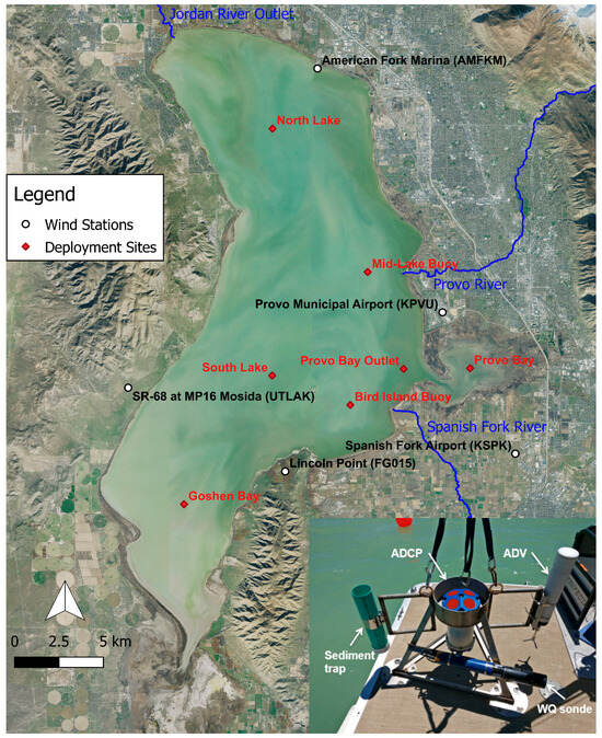
Utah Lake is a large, shallow lake with a surface area of 380 square kilometers, average depth of 3.2 m and wind fetch up to 33 km (Figure 1). The lake is a carbonate-dominated system characterized by enriched nutrient concentrations that result in high productivity, low transparency and the common occurrence of nuisance algal blooms and harmful cyanobacterial blooms [36,37]. The lake has a large open-water area and two embayments, Provo Bay and Goshen Bay, each with distinct morphometric and sediment characteristics (Figure 1). Inflows to the lake are from three rivers and several creeks that drain an 11,357 km2 watershed comprising mountainous headwaters and agricultural or urbanized valleys. With one outlet (Jordan River), Utah Lake is managed as a water supply reservoir while also providing flood storage which results in annual fluctuations in water surface of up to 1 m and multi-year fluctuations of up to 3 m [38]. Based on the Provo Municipal Airport weather station data from 2018 to 2025, the mean monthly air temperature, dew point, rainfall and wind speed for the range of months of deployment are: April—9.4 °C, −1.1 °C, 2.8 cm, 3.0 m/s; July—23.9 °C, 7.2 °C, 1.3 cm, 2.7 m/s; and October—10.0 °C, 1.1 °C, 3.0 cm, 2.5 m/s. Provo Bay has emergent aquatic vegetation (EAV) and high organic content sediments, while Goshen Bay has consolidated cohesive sediments. Non-native carp were introduced into the lake in the 1880s, resulting in a significant ecological shift that threatens the endangered native June Sucker and causes sediment resuspension via bioturbation.
Figure 1.
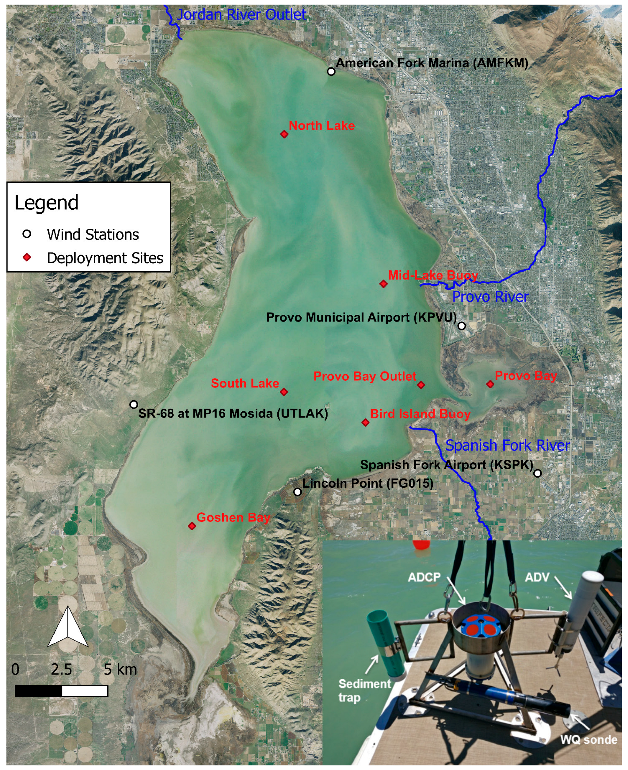
Instrumentation deployment sites (aerial image courtesy of the United States Geological Survey).
2.2. Data Collection
Sediment resuspension has previously been estimated in other lakes utilizing several different approaches, including optical sensors, sediment trap measurements, mass balance calculations and modeling formulations [39,40]. In this study, near-lake-bottom optical measurement of turbidity was used as a surrogate for sediment resuspension and deposition. Turbidity is an optical characteristic that represents the amount of light that is scattered by material in the water when light is shined through the water and is reported in formazin nephelometric units (FNU) or nephelometric turbidity units (NTU) in this study.
Key hydrodynamic, water quality and sedimentation properties were measured by deploying multiple instruments on the lake bottom. The instrumentation was deployed for 2–4 weeks at multiple sites within the open water and embayments that represent varying water depths, lake fetches, and sediment conditions (Figure 1 and Table 1). A stainless-steel mount was fabricated for the instrumentation (Figure 1). We used a YSI Inc. (1700/1725 Brannum Lane, Yellow Springs, OH 45387, USA) EXO2 multi-parameter water quality sonde located approximately 6 inches above the lake bottom with sensors that measured water temperature (±0.01 °C), specific conductance (±0.5% or 0.001 µS/cm), pH (±0.1), dissolved oxygen (±1% or 0.1 mg/L), turbidity (±3% or 0.3 FNU), chlorophyll a (±0.01 RFU), and phycocyanin (±0.01 RFU) every 15 min. Chlorophyll is a pigment that provides an estimate of the concentration of green algae in the water column and is reported in relative fluorescence units (RFU). Phycocyanin is a pigment that provides an estimate of the concentration of blue-green cyanobacteria in the water column and is reported in relative fluorescence units (RFU). Chlorophyll and phycocyanin are components of turbidity.
Table 1.
Lake bottom instrument deployments.
In addition to the instrumentation deployed at the lake bottom, several buoy sites with near-surface water quality parameters and meteorological variables were maintained by the Utah Division of Water Quality (Figure 1). The water quality sondes at each site recorded water temperature, specific conductance, pH, dissolved oxygen, turbidity, chlorophyll a, phycocyanin, and fine dissolved organic material (FDOM) on a 15 min time interval. A weather station was added to the Mid-Lake site in 2020 that measured air temperature, relative humidity, barometric pressure, solar radiation, and wind speed and direction. Wind speed and direction data was also obtained from other entities at several near-shore sites (Figure 1).
Sediment cores of 30 cm depth were collected at each of the instrument deployment sites. The following sediment physical properties were characterized through laboratory tests, including bulk density (ASTM D7263 [41]), organic content (ASTM D2974 [42]), water content (ASTM D2974 [42]), and grain size distribution, using the hydrometer method (ASTM D7928 [43]). The tests were run on sediment depths of 0–5 cm, 5–15 cm and 15–30 cm. The sediment shear strength was measured in situ at each site using a shear vane per the ASTM D2573–08 Standard Test Method for Field Vane Shear Test in Cohesive Soil [44].
2.3. Turbidity Modeling
Machine learning regression techniques were applied to predict turbidity, the response or independent variable, based on a set of explanatory variables, as described below.
2.3.1. Data Selection and Preparation
The list of explanatory variables considered for the prediction of turbidity is summarized in Table 2. These variables were selected based on their mechanistic connection to sediment resuspension and settling. Wind speed, wind direction, water depth and fetch factor into wave height and shear stress exerted on the lake bottom. Fetch is the length of open water that wind travels over to reach a particular location on the lake for a given wind direction. Fetch length at the location of the instrument deployments was calculated at 22.5-degree intervals using a wind fetch calculation tool developed for ESRI (380 New York St, Redlands, CA, USA) ArcGIS ArcMap 10.2 by the USGS [45]. Shear stress was derived from wind speed, wind direction, water depth and fetch utilizing methods for shallow waters described in the United States Army Corps of Engineer’s (USACE) Shore Protection Manual [46]. For a full description of shear stress estimation, refer to Appendix A.1. Shear stress is included as an explanatory variable in this analysis for comparison to models utilizing only the directly observed variables. The sediment characteristics of bulk density, D80 grain size, shear strength, organic content, clay content and organic content affect the erosivity and settling rate of the lake sediments. Chlorophyll a and phycocyanin provide estimates of the algal and cyanobacterial contents in the water column.
Table 2.
Summary of explanatory variables.
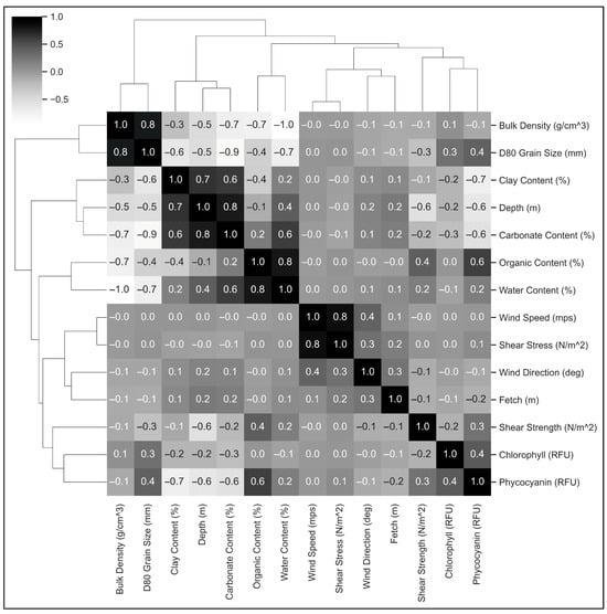
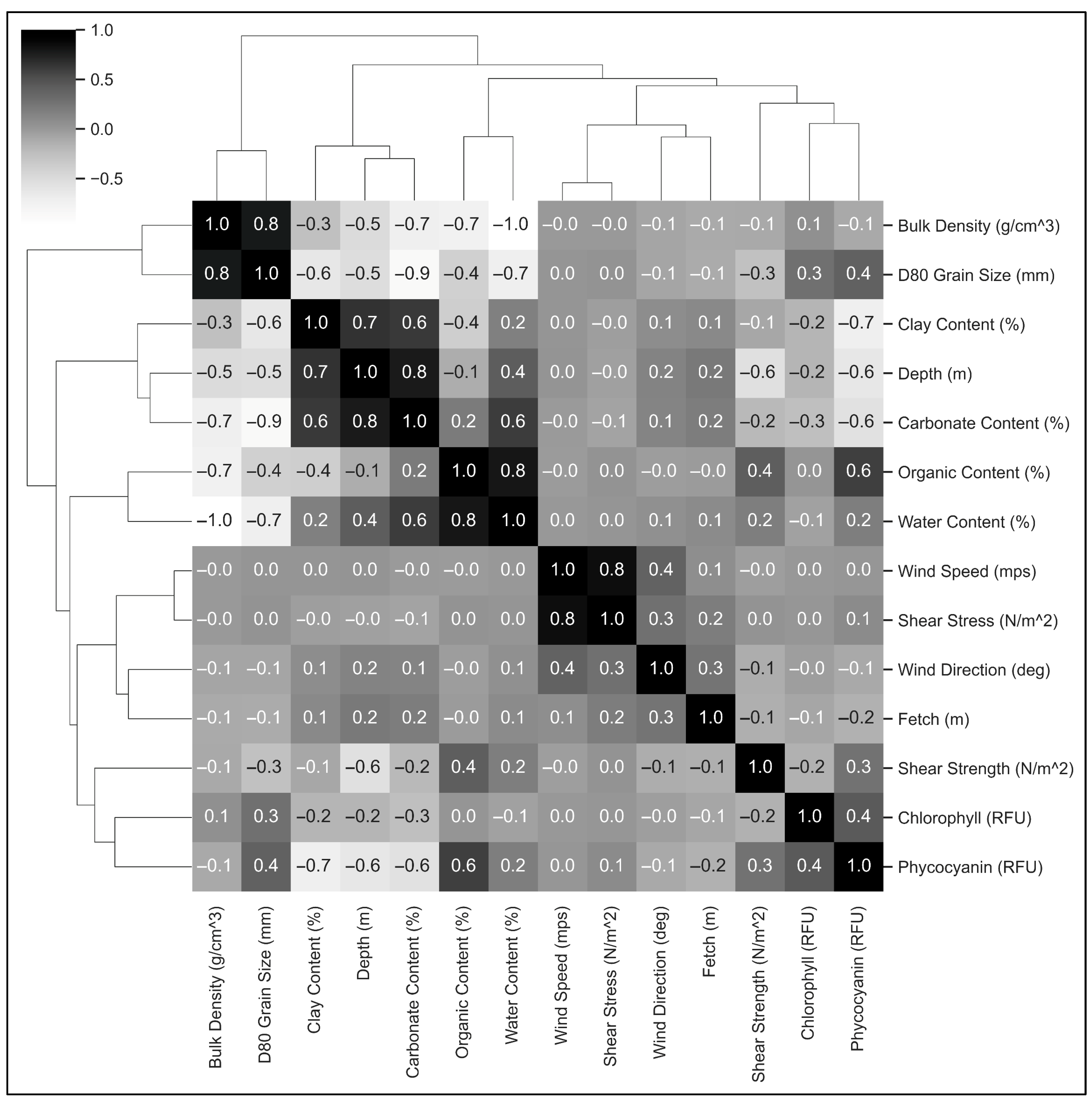
Collinearity in regression models occurs when there is strong correlation between predictor variables. The inclusion of correlated variables may convey redundant information, increase model complexity, and reduce model performance. A hierarchically clustered heatmap (with clustering method: “average” and distance metric: “Euclidean”) of the Pearson correlation matrix was constructed to evaluate potential collinearity between the explanatory variables (Figure 2). D80 grain size exhibited high positive correlation with bulk density and high negative correlation with carbonate content; therefore, grain size was dropped from the regression models. Shear stress and wind speed also exhibited high correlation and statistical significance (r = 0.846, p < 0.001); however, these were not intended to be included in the same regression model anyway. Interestingly, clay content and carbonate content had high correlation with water depth, but these variables were maintained in the model since this was likely an artifact of the relatively small number of deployments. Principal component analysis (PCA) is a commonly applied approach to reduce dimensionality and multicollinearity [47,48], but that was found to not to be necessary or beneficial for this study.
Figure 2.
Pearson correlation matrix for explanatory variables.
Several sets of explanatory variables were evaluated (Table 2). In Set 1 all directly observed variables were included in the regression. In Set 2 chlorophyll and phycocyanin were removed due to the potential collinearity with turbidity and potential lack of availability for making the prediction. In Set 3, the Set 2 variables were included with shear stress instead of wind speed, wind direction, fetch and depth. The objective of Set 3 was to evaluate the use of a mechanistically based, derived variable in comparison to direct observations. Finally, in Set 4, the Set 2 variables were included with data from the Provo Bay site removed due to its distinct characteristics.
In supervised machine learning, the explanatory and dependent variable input data is split into a training set, which is used to build the model, and a testing set, which is used to evaluate model performance with an independent data set. For this study, the input data utilizing data collected from all the instrument deployments combined was split into the training and testing data sets utilizing a random 75–25 split. Each of the models considered the same explanatory variables and inputs for training and prediction purposes.
Machine learning models generally perform better if the explanatory and dependent variables are normalized and scaled. The types of data standardization and normalization employed for this study are summarized in Table 2. The MinMax Scaler scaled each feature to the dimensionless range 0 to 1. The Power Transformer utilized the parametric, monotonic Yeo–Johnson transform to map the variable to approximate a Gaussian distribution to stabilize variance and minimize skewness.
2.3.2. Machine Learning Regression Methods
Near-bottom turbidity was predicted utilizing four machine learning regression techniques, including random forest (RF), histogram-based gradient boosting (HBGB), support vector regression (SVR), and multi-layer perceptron (MLP). The algorithms in SciKit-Learn Python package Version 1.3.2 [49] (Pedregosa et al. 2011) were used for each estimator. Hyper-parameters are arguments that are passed to the constructor and are not directly learnt by each algorithm. Therefore, a parameter grid search was performed to determine the optimal set of hyper-parameters to fit each model based on the cross-validation score.
Decision trees perform a series of binary recursive splits of the explanatory variables that result in a tree with branches. Ensemble methods, such as random forests and gradient-boosted trees, aggregate the results of individual decision trees to correct for the model overfitting prone to individual regression trees. Random forest regression constructs the model by applying random sub-samples of the input data to an ensemble of individual decision trees [50]. The hyper-parameter that was optimized was the number of decision trees in the forest.
Histogram-based gradient boosting regression is a variant of general gradient boosting techniques that sequentially add training sets which correct for errors in prior training sets, thereby boosting weak learners into strong learners [51]. The HBGB algorithm bins continuous input variables into a discrete number of groups, which reduces the long model training time inherent in gradient boosting. The hyper-parameters that were optimized include the maximum number of iterations of the boosting process and the maximum number of leaves for each tree.
Support vector machine maps the continuous data points non-linearly in N-dimensional space based on the number of features and identifies the hyperplane that best fits the training data [52]. SVR is less susceptible to local optimal error minima and thus more generalizable globally. The hyper-parameters that were optimized include the kernel type, the regularization parameter C, and the kernel coefficient gamma.
Artificial neural networks (ANNs) emulate the structure of animal brains with nodes (neurons) that are grouped into a series of layers: an input layer, one or more hidden layers, and an output layer [53]. The multi-layer perceptron regressor uses multiple hidden layers comprising a perceptron, backpropagation of errors, an identity function in the output layer, and a square error as the loss function. The hyper-parameters that were optimized include the activation function for the hidden layer, the solver for weight optimization, the hidden layer sizes (number of hidden layers and number of neurons per layer), and the maximum number of iterations until convergence.
Four metrics were output to evaluate the performance of the estimator: explained variance score (EVS), Kling–Gupta Efficiency (KGE), percent bias (PBIAS), and mean absolute error (MAE). The EVS is similar to the coefficient of determination (R2) but does not penalize for bias, with the best possible score of 1. KGE is similar to Nash–Sutcliffe Efficiency (NSE) and varies from -infinity to 1, with a perfect fit being 1. PBIAS measures whether the model is consistently over- or under-predicting the observed values. The more traditional statistical approaches, simple linear regression (LR) and polynomial regression (PR), which extends simple linear regression through the use of a basis function, were included in this study as a baseline for comparison to the machine learning techniques.
Permutation feature importance was conducted to evaluate the relative importance of each explanatory variable for the performance of each model. Permutation feature importance is defined as the decrease in model score when an explanatory variable is randomly shuffled. The importance of an explanatory variable is specific to a particular model and not reflective of the intrinsic predictive power of that variable.
3. Results
3.1. Observed Data
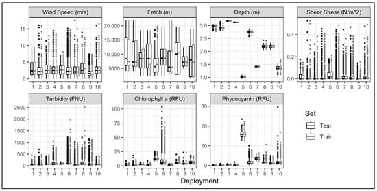
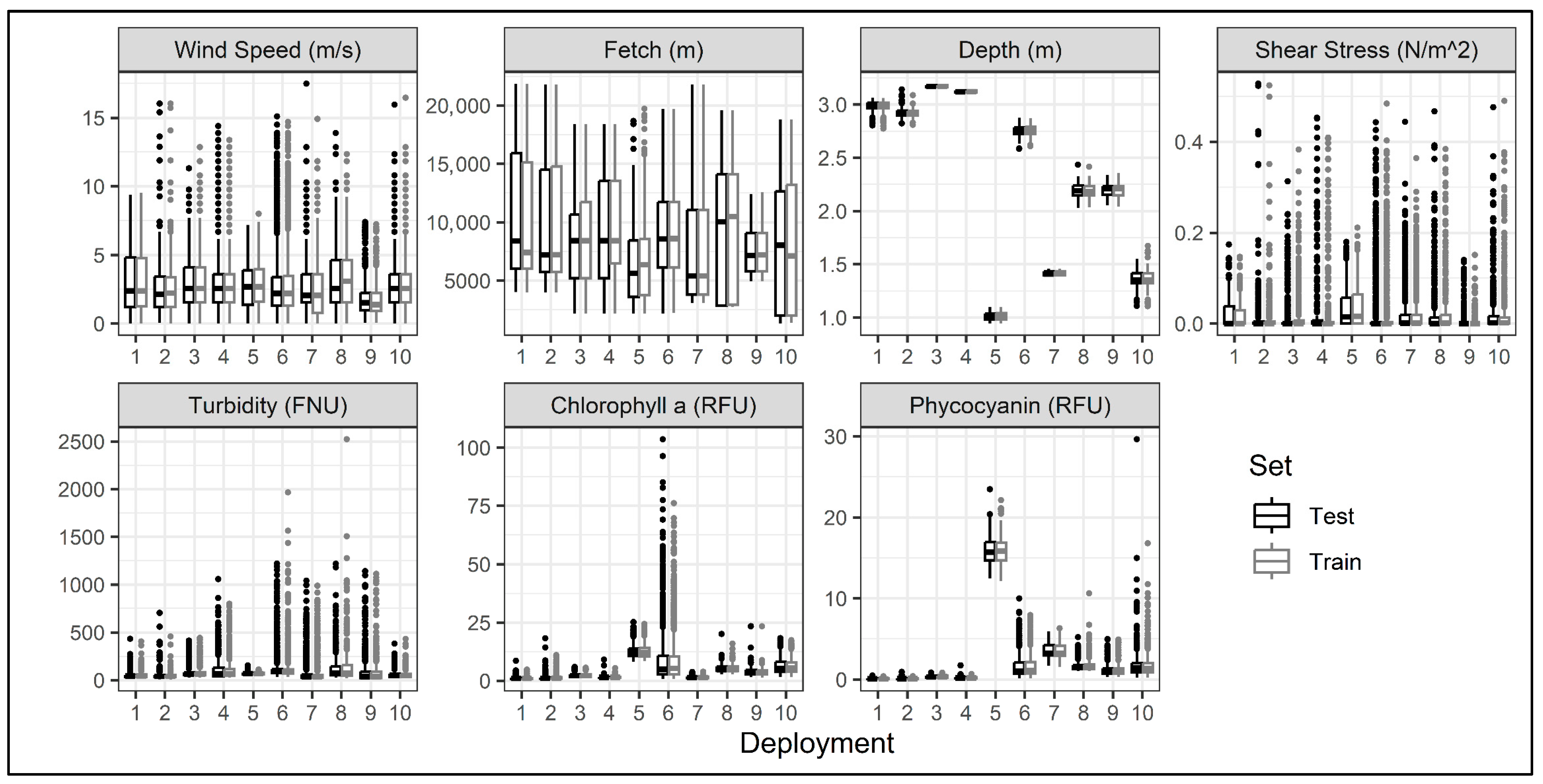
The water quality sonde recorded 15,470 data points during the ten deployments. The physical and chemical properties of the lake bottom sediments were similar at each of the open-water sites, but different in the embayments (Table 3). The surface-layer bulk density was lowest and the organic content and water content were highest at the Provo Bay site, whereas the surface-layer bulk density was highest at the Goshen Bay site. Based on the in situ measurements using the shear vane, the Goshen Bay site had the highest surface shear strength, followed by Provo Bay. The median of observed wind speeds was similar for all of the deployments, whereas Deployments 1, 5 and 9 experienced lower maximum wind speeds and shear stresses than the other deployments (Figure 3). An increase in turbidity in response to wind events was observed during all of the deployments (Figure A1 in Appendix A.2), with maximum turbidity ranging from 156 to 2522 FNU (Figure 3). During quiescent periods, the turbidity decreased asymptotically (Figure A1 in Appendix A.2), with the minimum turbidity ranging from 7 to 44 FNU and Provo Bay exhibiting the highest minimum turbidity (Figure 3). Refer to the Appendix A.2 for additional results and a discussion regarding the observed linkage between wind speed and direction, fetch, shear stress and turbidity. Except for Deployments 5, 6 and 10, minimal algal and cyanobacterial growth was observed in the water column near the lake bottom (Figure 3). The distribution between the training and testing data sets was similar, with higher extreme values of turbidity in the training set and of chlorophyll in the testing set (Figure 3).
Table 3.
Sediment physical properties.
Figure 3.
Box whisker plots of observed variables and calculated shear stress for all deployments.
3.2. Turbidity Prediction
Models that predict turbidity were built using each of the machine learning techniques described above in Materials and Methods and various combinations of the explanatory variables.
3.2.1. Model Performance
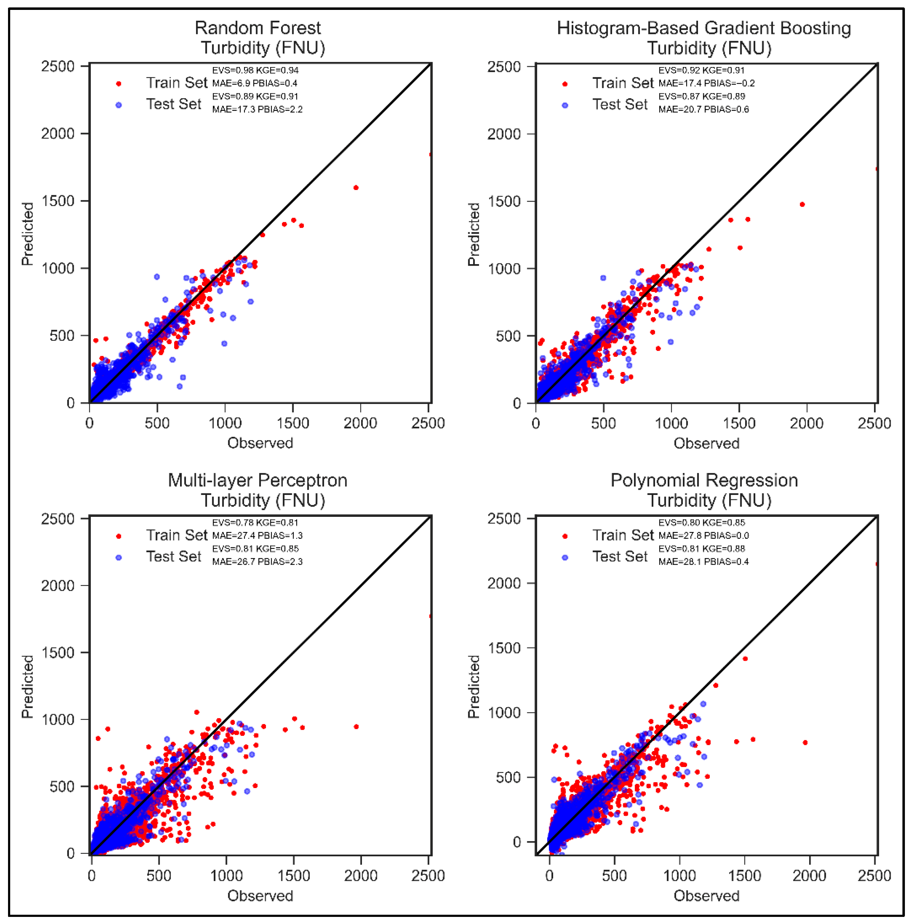
The optimized hyper-parameters selected for each model are summarized in Table 4. The model performance metrics explained variance score (EVS) and mean absolute error (MAE) for turbidity prediction using the test data are summarized in Table 5. Except for SVR, the machine learning techniques had superior model performance compared to simple linear regression (Table 5). The decision tree approaches RF and HBGB had the highest scores (0.89 and 0.86, respectively) and least error (17.3 and 21.3, respectively) when all explanatory variables were included. The polynomial regression and MLP models performed similarly well, but there was some improvement in prediction capability through the use of the decision tree methods. The SVR estimator exhibited poor performance, with a worse model fit than simple linear regression.
Table 4.
Machine learning hyper-parameters.
Table 5.
Regression model performance metrics on the test set for explanatory variable sets.
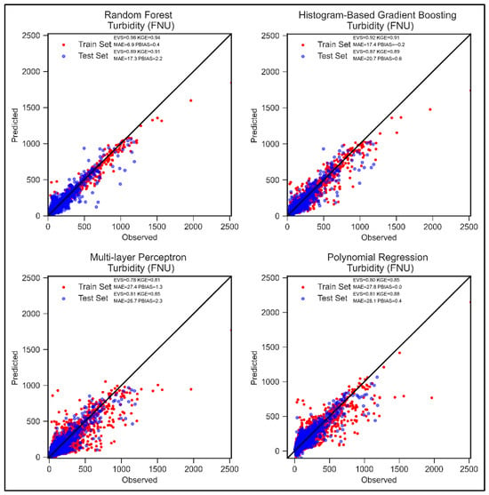
Model performance decreased considerably when the explanatory variables chlorophyll and phycocyanin were removed, with the most pronounced effect on the MLP model (EVS reduced from 0.81 to 0.43). Model performance was also dramatically degraded when the directly observed variables wind speed and direction, water depth, and fetch were replaced with the derived variable shear stress, whereas there was a negligible difference in model performance when the Provo Bay site was removed (Table 5). The models tended to underpredict the highest turbidity spikes, but performed consistently at the low and mid ranges (Figure 4).
Figure 4.
Scatter plot of predicted versus observed for each estimator with 1:1 line.
3.2.2. Explanatory Variable Importance
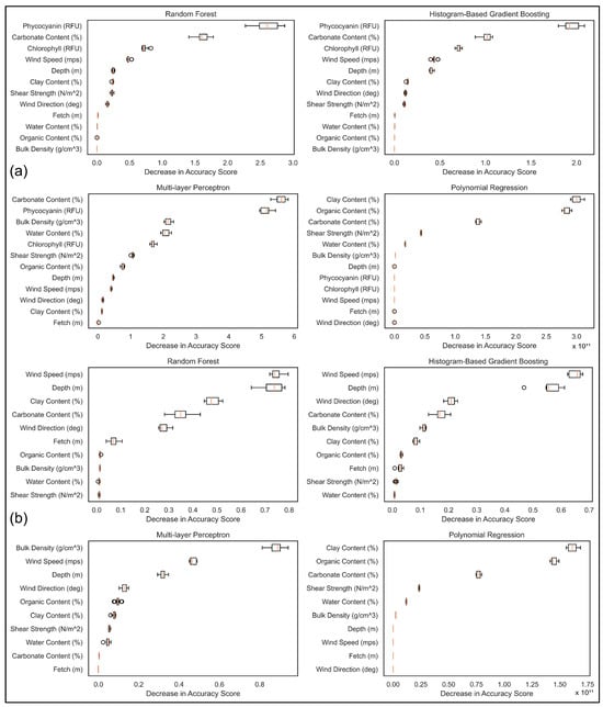
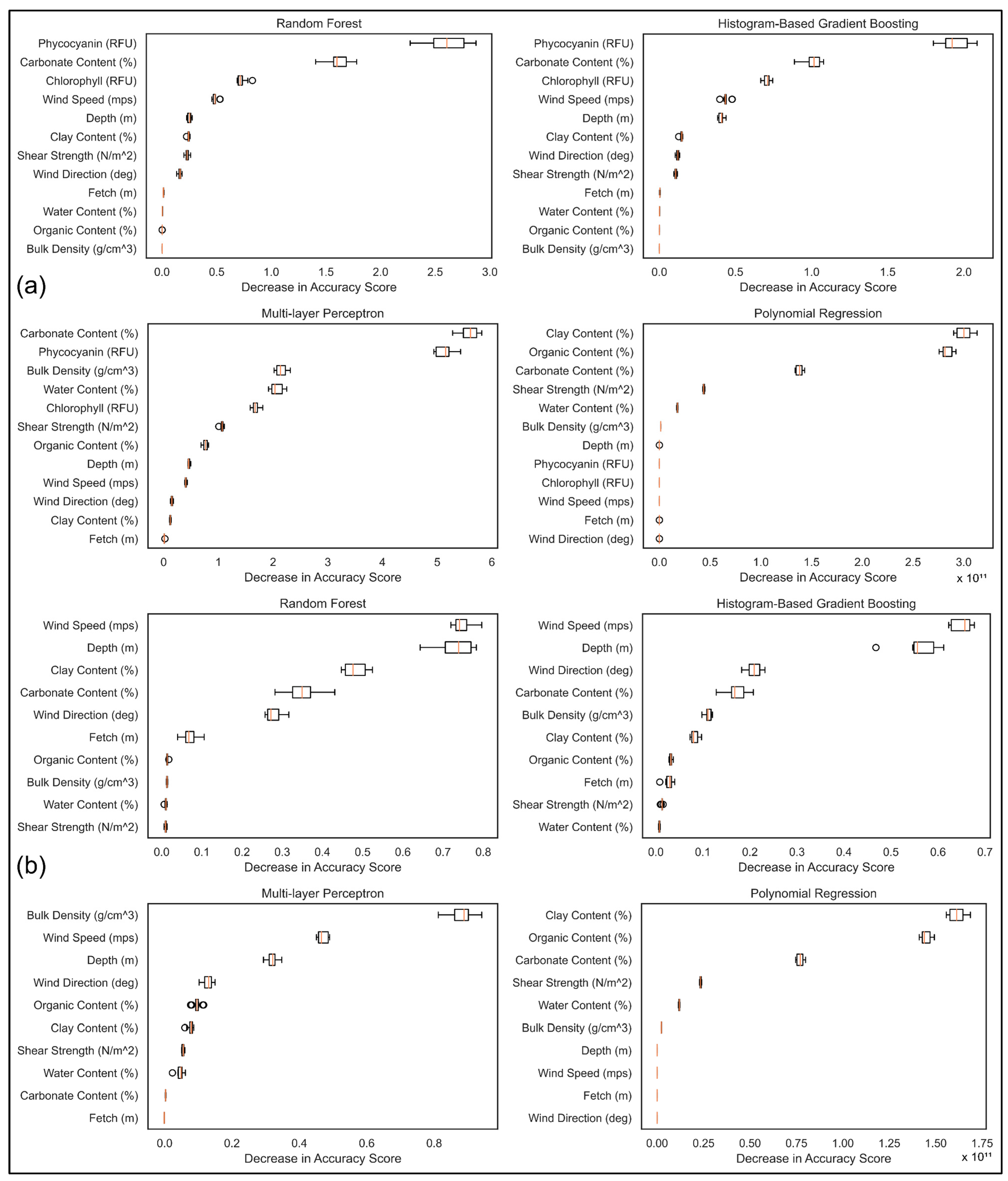
For the decision tree models, RF and HBGB, as well as the MLP model, the explanatory variables phycocyanin and carbonate content had the greatest impact on the accuracy score based on the permutation importance test (Figure 5a). The next most important variables in the decision tree models were chlorophyll and wind speed, with fetch, water content, bulk density and organic content having little or no importance to model performance. Sediment characteristics were the most important predictors in the polynomial regression, with the hydrodynamic variables (depth, wind speed, wind direction and fetch) and biological variables (chlorophyll and phycocyanin) having little or no importance.
Figure 5.
Permutation importance of explanatory variables using the test set for (a) all directly observed variables and (b) directly observed variables excluding chlorophyll and phycocyanin.
When chlorophyll and phycocyanin were removed from the models, wind speed and depth were the most important predictors in the RF and HBGB models and bulk density in the MLP model (Figure 5b). Since chlorophyll and phycocyanin were unimportant in the polynomial regression model, their removal had little impact.
4. Discussion
4.1. Machine Learning Model Comparison
Of the machine learning regression estimators evaluated in this study, the decision tree (DT) approaches RF and HBGB exhibited the best model performance, with EVSs of 0.89 and 0.86, respectively. Several previous studies also successfully used hydrodynamic measurements and sediment properties to predict sediment transport using a DT approach [54,55].
The artificial neural network (ANN) method MLP performed slightly worse than the decision tree models and similar to the simpler polynomial regression estimator (Table 5). Oehler et al. [54] also found that a boosted regression tree (BST) model exhibited better performance than an ANN in the prediction of near-bed suspended sediment concentration in shallow coastal waters based on hydrodynamic observations and median grain size. In this case study, the ANN model’s performance may have been inhibited by a somewhat small data set for model training that limited optimization of the hyper-parameters specifying the number of hidden layers and the number of neurons in each hidden layer. However, ANN models continue to merit consideration, as model performance was nearly as good as the DT models and they are not as prone to overfitting. Yoon et al. [56] successfully applied an ANN model to predict sediment suspension in a large-scale laboratory experiment under erosive and accretive beach conditions.
The SVR estimator exhibited poor performance, with a worse model fit than simple linear regression. This result was not expected, as previous studies have successfully applied support vector machine models to the prediction of turbidity in coastal waters [57] and sediment transport in rivers [30]. Wang et al. [57] achieved similar model performance using an ANN and SVR to predict turbidity in coastal waters, though SVR overestimated low turbidity and underestimated high turbidity.
The ML models generated by this study could be applied to any independent data set to predict turbidity. The results of this study indicate that DT and ANN approaches show significant promise in predicting sediment transport in shallow waters and warrant further research. It is not clear how well the ML techniques and specific models would perform in other shallow lakes with divergent hydrographic and sediment characteristics; however, they show promise for wider application based on performance in this case study and results from previous studies, and therefore merit further consideration and investigation. The ANN approach would likely benefit from a larger data set to improve optimization of the hyper-parameters for hidden layer number and size.
4.2. Drivers of Sediment Dynamics
An increase in turbidity in response to wind events was observed during all the deployments, with an asymptotic decrease in turbidity during periods with lower wind speeds (Appendix A and data from article). Similar findings were found in the Salton Sea in California, where turbidity was found to be proportional to wind speed and water depth [58], and in shallow Lake Markermeer, where total suspended matter did not show a positive response during low wind speeds [59]. Each deployment had an apparent minimum turbidity threshold, potentially due to the buoyancy, inter-particle attraction and low critical shear stress of deposition for the remaining portion of the suspended seston. Provo Bay had the highest minimum turbidity of the deployment sites, which is likely attributable to the protected hydrographic setting and higher primary productivity of the bay, which resulted in a higher proportion of organic content and lower settling velocity of the suspended sediments. Bioturbation by carp may also play a role in the higher minimum turbidity in Provo Bay.
When the directly observed variables wind speed and direction, fetch (function of wind direction and site position), and water depth were replaced with the shear stress due to wave action estimated using the USACE formula, model performance was somewhat degraded (Table 5). The wave properties and resultant shear stresses on the lake bottom are dependent on the duration and magnitude of the wind and simplifying assumptions are necessarily made in the calculation. Also, a time lag between shear stress and sediment resuspension was observed (see Appendix A and data from article), which may have confounded it as a predictor variable. This also applied to fetch, which had less or equal importance than wind direction in all the models (Figure 5). The finding that shear stress and fetch were poorer predictors than the underlying directly observed variables indicates the limitations and challenges associated with estimating complex environmental properties using mechanistic equations and the opportunities presented by non-physically based ML regression techniques.
Provo Bay is a more protected embayment with physical, chemical and biological attributes that are distinct from the main lake and Goshen Bay. With shorter fetch and shallower depth, Provo Bay functions more like a small lake or wetland and is much less susceptible to sediment resuspension events. Removing the Provo Bay site from the regression analysis, however, did not have an appreciable effect on model performance (Table 5), indicating that the underlying drivers of sediment resuspension are more generally applicable to at least the hydrographic and sediment variability within Utah Lake.
The relative importance of the explanatory variables used to predict turbidity response depended on the ML regression technique employed (Figure 5). For instance, phycocyanin and chlorophyll had high importance in the DT and MLP models, but almost no influence on the PR model performance. While bulk density had the third highest impact on the accuracy score for the MLP model, it had no importance in the DT models, which emphasizes how dependent variable importance is on the specific model. Chlorophyll and phycocyanin were amongst the most important variables in the DT and MLP models, which is potentially partially due to auto-correlation effects associated with organic matter being a component of turbidity. With chlorophyll and phycocyanin removed, the hydrographic and meteorological variables (water depth, wind speed, and wind direction) moved up in importance in the DT and MLP models, as would be expected from the physically based explanation of the causes of sediment resuspension and deposition (see Appendix A and data from article for additional discussion of the mechanics).
Regarding the sediment properties, carbonate content was of high importance in the DT and MLP models. Utah Lake is a calcareous system with high carbonate content in the sediments in its open waters (62.7–78.0%), but with significantly lower carbonate content at the more protected sites (11.5–45.6%). Calcite and apatite form flocs that settle and deposit slowly, consolidate poorly and erode easily. Therefore, carbonate content was a good discriminator of the potential for erosion between the sites. Clay content was more important to the DT models, whereas bulk density was more important to the MLP estimator. Each of these variables has a strong mechanistic connection to the erosion and deposition of cohesive sediments [60]. Many laboratory experiments have attempted to correlate critical shear stress to the physical properties of sediments. However, since flume studies inadequately replicate the hydrodynamic and sediment characteristics of the natural environment, and due to the challenge and expense of reliably measuring critical shear stress in situ, lake-specific empirical formulations that relate sediment characteristics such as bulk density to critical shear stress have been developed [22,61].
Although the relative importance of a variable is specific to a model and is not generalizable, when a variable is important to multiple well-performing models, it can be inferred that it has direct connections to mechanistically based processes. Therefore, water depth and wind speed and direction, as well as chlorophyll and phycocyanin, were found to be good predictors of turbidity, whereas the lake bottom sediment properties had mixed importance that was dependent on the particular ML technique employed.
When all the explanatory variables were included, the estimators other than SVR predicted 81 to 89% of the variability in the turbidity data. Other potential sources of variance that could be included in future studies are as follows: uncertainty associated with the measurement of turbidity by the optical sensors, advection of sediment within the lake through hydrodynamics and currents, spatiotemporal variability of wind over the lake surface, bioturbation of sediments by invasive carp, and other biological and chemical characteristics of cohesive sediments that affect erodibility (i.e., sodium adsorption ratio and biogenic structures such as biofilms).
4.3. Implications on Lake Management and Restoration
Wind-induced turbulence and sediment dynamics in shallow lakes affect several important ecological processes, including internal phosphorus cycling [62,63,64,65,66], algal and cyanobacterial growth in the water column [6,10,67], and macrophyte establishment [21,68,69]. Sediment resuspension affects the potential for a shallow lake to transition from a phytoplankton-dominated turbid stable state to a macrophyte-dominated clear stable state [16]. Suspended sediment in the water column inhibits the establishment of submerged aquatic vegetation by creating unstable sediment substrates for root development [70] and by limiting the amount of light that reaches the benthic zone [71], resulting in a planktonic-dominated system [72]. The restoration of benthic dominance of primary productivity was found to be possible in Utah Lake, with a 0.9 m increase in water clarity in the open water and a 0.3 m increase in the wind-protected bays [73]. The lack of SAV results in a positive feedback loop of increased shear stress on the lake bottom, enhanced sediment resuspension, poorer water clarity, and less favorable conditions for the establishment of benthic vegetation.
This study found that shear stress on the lake bottom from wave action was a good predictor of and resulted in sediment resuspension at various sites throughout the lake, regardless of the sediment characteristics and physiographic setting of the site. Of the primary factors found to contribute to the turbidity in the lake (water depth, fetch length, wind conditions, and sediment properties), water depth is the most feasible to manage on a lake-wide basis. Utah Lake is currently managed as a reservoir with the dual objective of supplying irrigation and industrial process water to downstream users and balancing flooding along the lakeshore and the Jordan River downstream. In addition, the lake has not been assigned a conservation pool or a minimum water level by the Utah State Engineer. Subsequently, the lake level fluctuates several feet intra-annually for water supply and recedes inter-annually during years when outflows exceed inflows. The lower water depths resulting from these reservoir management practices enhance sediment resuspension and inhibit sediment deposition, partially contributing to the turbid conditions predominating in the lake.
Lake fetch and wind conditions are not as easily manipulated as water depth, requiring engineered solutions such as breakwaters to provide more sheltered conditions from wave action. Likewise, enhancing sediment stability by establishing SAV throughout the lake would be challenging given the frequent wave action on the lake bottom. These may not be feasible or desirable management actions to implement in the open waters, but restoration efforts could be focused on embayments that naturally have some protection from the wind. The resuspension of sediments was reduced in Provo Bay by decreased shear stresses resulting from both the presence of emergent aquatic vegetation (EAV) and the smaller fetch length of the embayment. The Goshen Bay site, which had no aquatic vegetation and had limited protection from the wind, had a similar response in turbidity as the open-water main lake sites. The reestablishment of both SAV and EAV in portions of the lake would result in reduced sediment resuspension, enhanced sediment deposition and lower turbidity locally and throughout the lake.
5. Conclusions
This study applied selected supervised machine learning regression models to predict turbidity utilizing meteorological, hydrodynamic, water quality and sediment data collected at various sites throughout Utah Lake. The models’ performance and explanatory variable importance were evaluated and compared to improve the prediction of water clarity and understanding of sediment dynamics in a large, shallow lake in a semi-arid setting. The primary findings and conclusions of the study include the following:
- Decision tree estimators, particularly random forest and histogram-based gradient boosting, demonstrated the highest predictive performance, explaining 86–89% of the variability in turbidity when including all the explanatory variables. The artificial neural network estimator multi-layer perceptron and polynomial regression models also performed well (81%), whereas the support vector machine estimator exhibited poor predictive capability for this data set. The application of decision tree estimators to water clarity and sediment transport prediction has not previously been widely investigated and is a promising area of future study. The artificial neural network technique also has merit and, potentially, model performance would improve with a larger data set for model training and hyper-parameter optimization.
- Chlorophyll and phycocyanin were among the most influential predictor variables in the decision tree and artificial neural network models, along with wind speed and carbonate content. When chlorophyll and phycocyanin were removed, wind speed and direction and water depth were amongst the most important predictors in the decision tree and multi-perceptron models, which conforms with the physically based understanding of the primary drivers of sediment resuspension and deposition.
- Carbonate content was consistently a good predictor of turbidity across the models, which is likely due to the calcareous nature of Utah Lake, which has a high proportion of calcite and apatite in the sediments that are highly susceptible to erosion. The relative importance of the remaining sediment characteristics was dependent on the specific model. Bulk density was more important in the multi-perceptron model, whereas clay content was more important in the decision tree and polynomial regression models. Each of these characteristics are factors in the erosion potential of sediments, but quantifying their mechanistic effect on overall sediment dynamics is not well understood. Additional study into the relative importance of sediment properties to the prediction of sediment resuspension and deposition is recommended.
- The exclusion of Provo Bay, a protected embayment with sediment dynamics distinct from the main lake, from the regression analysis negligibly impacted the model performance, indicating that the turbidity prediction models are applicable to the heterogeneous conditions of Utah Lake and potentially more generally applicable to other large, shallow lakes.
Overall, the results demonstrate that the application of machine learning methods to predict water clarity in large, shallow lakes shows significant promise given the complex physical, chemical and biological factors and processes involved. Compared to mechanistic process-based models, these approaches require significantly less data preparation and computational resources and could therefore have greater utility for use in forecasting sediment resuspension and deposition, and future linkage to algal bloom formation. The machine learning models also help to elucidate the primary drivers of sediment dynamics, complementing the physically based understanding. In spite of the limitations related to data set size, the potential autocorrelation with chlorophyll and phycocyanin, and the absence of advective transport effects described previously, these predictive tools may support lake management strategies by providing rapid forecasts of turbidity responses to wind events and water-level changes, which are critical factors influencing sediment resuspension, nutrient cycling, and harmful algal bloom dynamics in shallow lake systems. Although the data set contains high-frequency measurements, the temporal coverage of individual deployments was limited. Additional long-term monitoring would further improve model robustness and generalizability. Future research should be directed at investigating the optimal regression estimator for this application, the most parsimonious set of explanatory variables that still result in accurate water clarity predictions, and the transferability of these models to other shallow lakes of varying sizes and physiographic settings. Specifically, additional research should aim to clarify limitations regarding transferability to lakes with different sediment composition, morphology, or hydrodynamics.
Author Contributions
Conceptualization, N.v.S. and M.B.; methodology, N.v.S.; formal analysis, N.v.S.; writing—original draft preparation, N.v.S.; writing—review and editing, M.B.; visualization, N.v.S.; supervision, M.B.; project administration, N.v.S. All authors have read and agreed to the published version of the manuscript.
Funding
This research received no external funding.
Data Availability Statement
All data, models, or code that support the findings of this study are available from the corresponding author upon reasonable request.
Acknowledgments
The sediment physical property tests were conducted by Han-Yan Li and Anwar Alsanea in Ramesh Goel’s environmental laboratory at the University of Utah. The in situ shear vane measurements were made by Steven Bartlett with assistance from Anwar Alsanea. The instrumentation mounting frame was fabricated at the shops at South Davis Sewer District by Eric Nemcek under the direction of Dal Wayment. The deployment of hydrodynamic instrumentation was conducted by Utah Department of Environmental Quality staff led by Marshall Baillie.
Conflicts of Interest
The authors declare no conflicts of interest.
Abbreviations
The following abbreviations are used in this manuscript:
| ANN | Artificial neural network |
| ASTM | American Society for Testing and Materials |
| D80 | Grain size of the 80th percentile particle |
| DT | Decision tree |
| EAV | Emergent aquatic vegetation |
| EVS | Explained variance score |
| FDOM | Fine dissolved organic material |
| FNU | Formazin nephelometric unit |
| HBGB | Histogram-based gradient boosting |
| LR | Linear regression |
| MAE | Mean absolute error |
| ML | Machine learning |
| MLP | Multi-layer perceptron |
| NTU | Nephelometric turbidity unit |
| PCA | Principal components analysis |
| PR | Polynomial regression |
| RF | Random forest |
| RFU | Relative fluorescence unit |
| SVR | Support vector regression |
| USACE | United States Army Corps of Engineers |
| USGS | United States Geological Survey |
Appendix A
Appendix A.1. Wave Parameter and Shear Stress Calculation
Shear stress on the lake bottom results from the interaction of current velocity, νc, and wave orbital velocity from wind waves, νw. The total bottom shear stress, , varies in magnitude and direction as a function of the interaction between currents and waves and can be calculated using the following [74,75]:
where is the shear stress due to water current velocities; and is the shear stress due to wave-induced orbital velocities.
The wind-generated water current velocity and associated lake bottom shear stress can generally be ignored in smaller shallow lakes (<10 km2), where sediment resuspension is dominated by wave-induced orbital velocity and shear stress [76]. The near-bottom shear stress resulting from waves was found to be the dominant factor in sediment resuspension in several large shallow lakes (>100 km2), including Lake Okeechobee [4,73], Lake Balatan [77], and Lake Taihu [17,33,63], and near-shore in Lake Tahoe [78]. The current velocity is the primary driver of advective transport of suspended sediments in the water column [74,79]. Therefore, the calculation of shear stress in this study only considered the effects of wave action and ignored the current velocity.
In order to estimate the shear stress due to wind waves, τw, for all deployments, including those without ADCP measurements, the wave parameters significant wave height Hs (m), wave period T (m), and wave length L (m) were calculated using empirical formulas from the United States Army Corps of Engineers (USACE) Shore Protection Manual for wind waves over shallow waters [46].
where g is acceleration due to gravity (m/s2); d is water depth (m); Uw is wind speed at 10 m above the ground (m/s); and F is the fetch length of wind (m). The wavelength in Formula (A4) was solved using the uniroot function in the plyr R package with a tolerance of 0.0001.
Shear stress due to wave action τw (N/m2) was calculated using laminar wave theory concept that when combined with the wave parameters, as determined by the USACE formulas, reduces to the following [80]:
Appendix A.2. Turbidity and Shear Stress
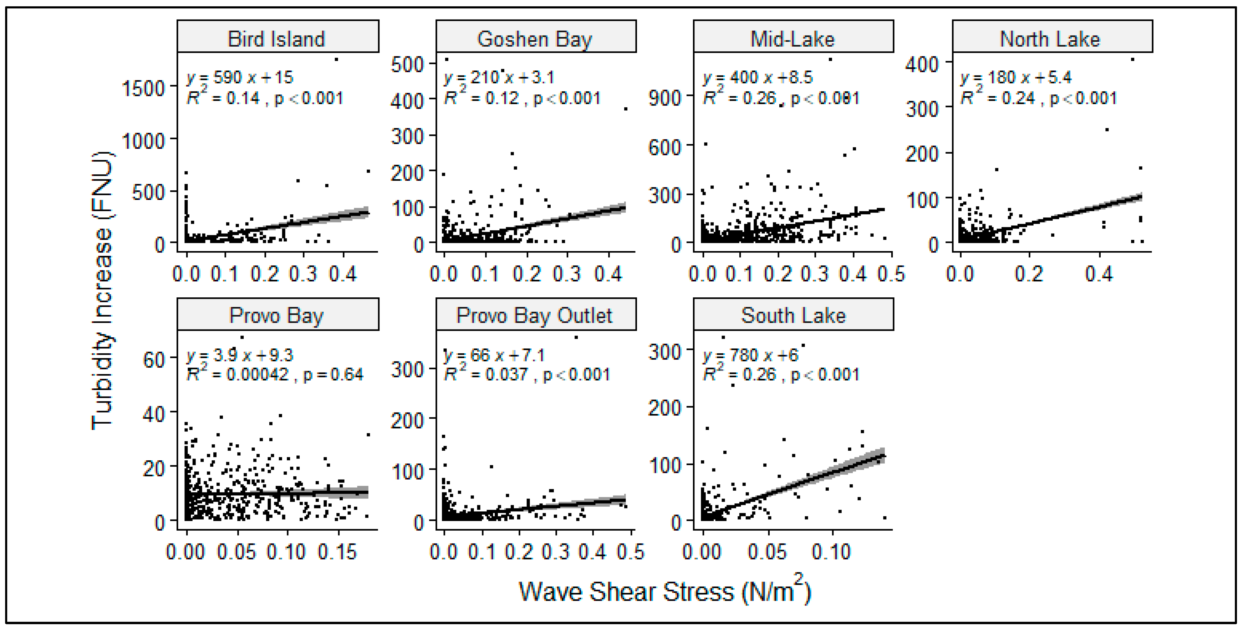
Sediment resuspension results when the bottom shear stress exceeds the critical shear stress of the lake sediments. A couple of issues confound the correlation between turbidity and shear stress. After sediment is resuspended during a wind event, it takes time for the suspended sediment to settle and deposit to the lake bottom. Therefore, high turbidity would be expected to occur during times of low shear stress. Additionally, a lag was observed between the wind measurement and the response in turbidity (Figure A1). To partially address these considerations, the correlation was performed only on those time steps that experienced increases in turbidity (i.e., resuspension). Turbidity increase was positively correlated with bottom shear stress due to wave action, with coefficients of determination (R2) that explained 12–26% of the variance for the open-water and Goshen Bay sites, while the Provo Bay and Provo Bay Outlet sites exhibited poor correlation between turbidity and shear stress (Figure A2). The poor correlation in Provo Bay may be due to the confounding influence of high primary productivity, whereas the poor correlation at the Provo Bay Outlet site may be due to advective transport of suspended sediments from Provo Bay to the open water and the high sand content of sediments at the site.
Figure A1.
Time series plot of turbidity and shear stress for 7/26/2019 (Deployment 2 North Lake).
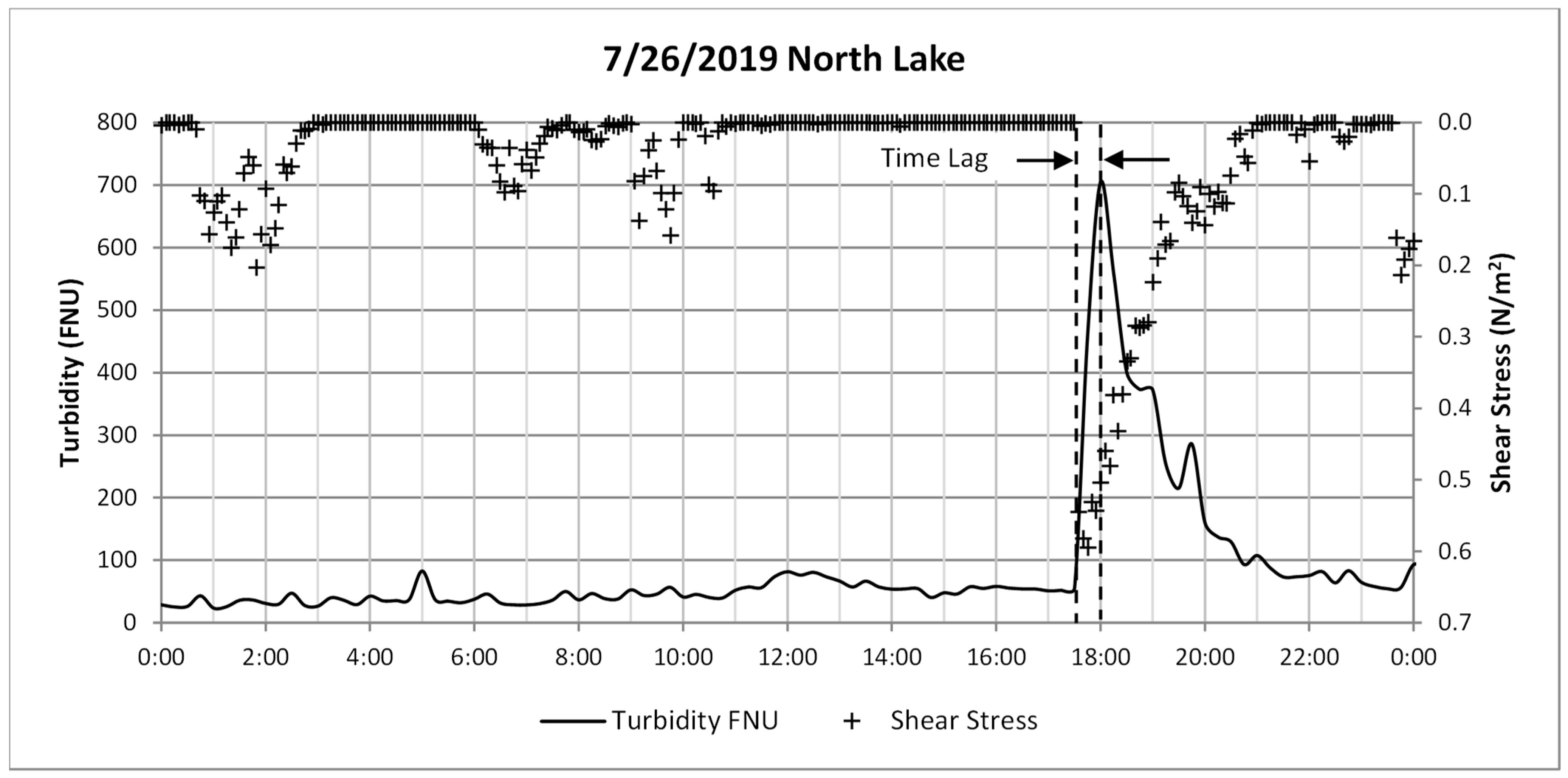
Figure A2.
Correlation plots between turbidity increase and shear stress due to wave action during time steps with increasing turbidity.
Appendix A.3. Turbidity and Primary Productivity
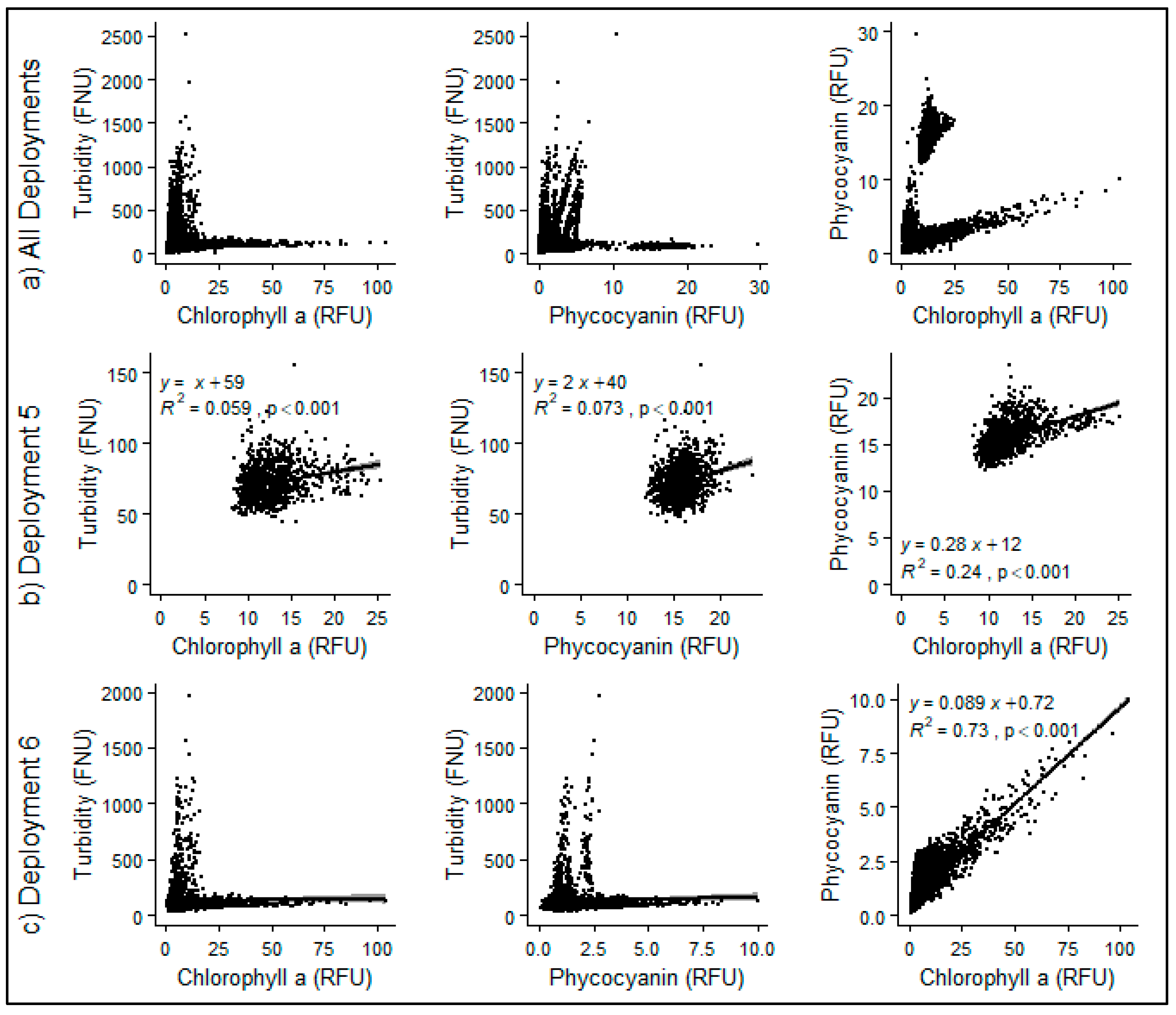
Primary productivity, as observed by the optical measures of chlorophyll a and phycocyanin, is a component of overall turbidity. Coincident diel fluctuations in the ratio of phytoplankton and cyanobacteria to turbidity indicated that during periods of low wind, the response in turbidity is primarily dependent on primary productivity (Figure A3). Except for the Provo Bay site, turbidity exhibited an inverse relationship to chlorophyll a and phycocyanin, i.e., when turbidity was high, chlorophyll a and phycocyanin were low and vice versa, whereas chlorophyll a and phycocyanin were positively correlated (Figure A4).
Figure A3.
Ratio of chlorophyll a and blue-green algae (BGA) to turbidity by deployment.
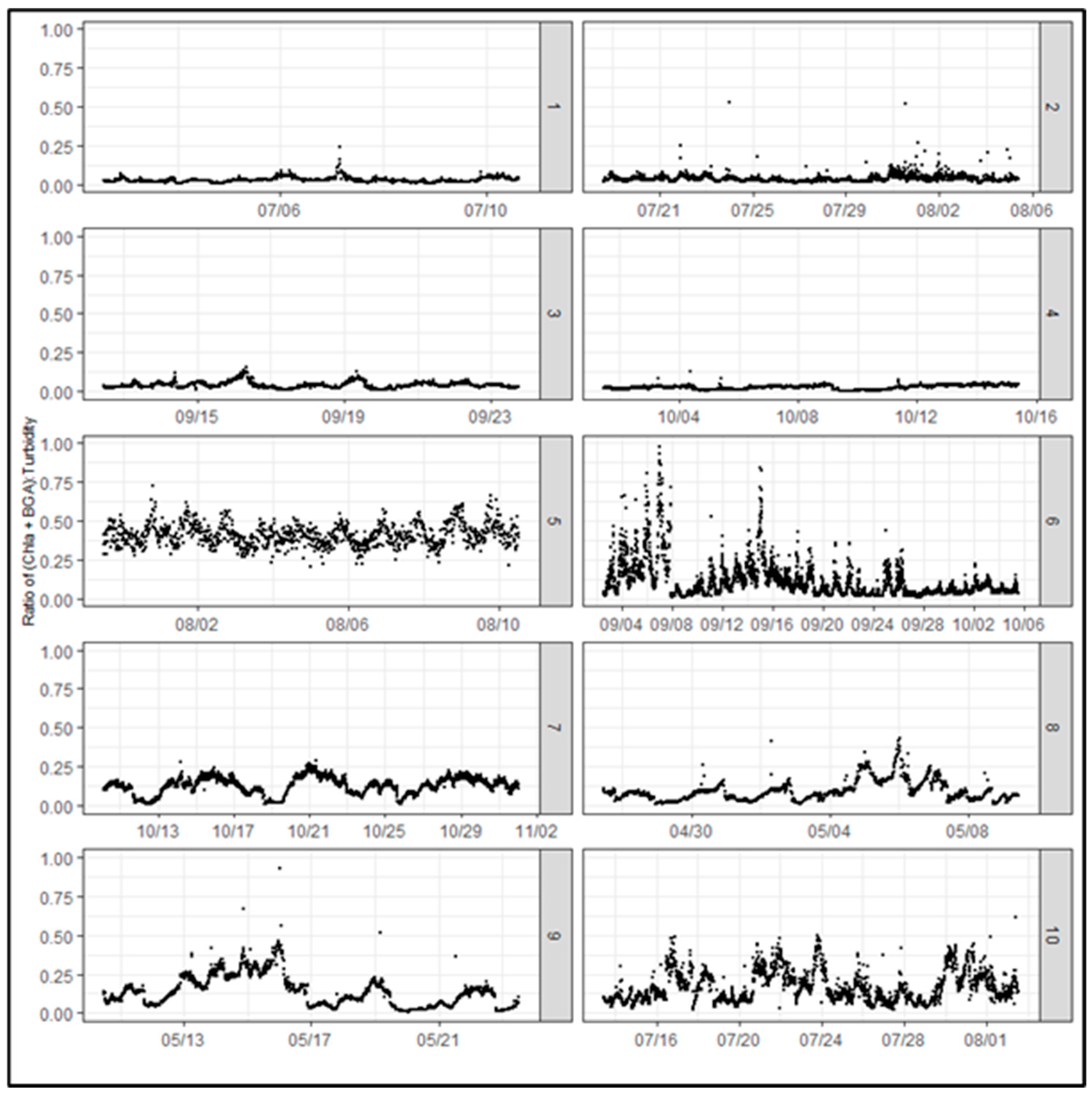
Figure A4.
Scatter plots of turbidity, chlorophyll a and phycocyanin. (a) All deployments; (b) Deployment 5 Provo Bay; and (c) Deployment 6 Mid-Lake.
References
- Aalderink, R.H.; Lijklema, L.; Breukelman, J.; Van Raa-phorst, W.; Brinkman, A.G. Quantification of wind induced resuspension in a shallow lake. Water Sci. Technol. 1984, 17, 903–914. [Google Scholar] [CrossRef] [Scilit]
- Hamilton, D.P.; Mitchell, S.F. An empirical model for sediment resuspension in shallow lakes. Hydrobiologia 1996, 317, 209–220. [Google Scholar] [CrossRef] [Scilit]
- Kelderman, P.; de Rozari, P.; Mukhopadhyay, S.; Ang’weya, R.O. Sediment dynamics in shallow Lake Markermeer, The Netherlands: Field/laboratory surveys and first results for a 3-D suspended solids model. Water Sci. Technol. 2012, 66, 1984–1990. [Google Scholar] [CrossRef] [Scilit]
- Ji, Z.-G.; Jin, K.-R. Impacts of wind waves on sediment transport in a large, shallow lake. Lakes Reserv. Res. Manag. 2014, 19, 118–129. [Google Scholar] [CrossRef] [Scilit]
- Scheffer, M. Ecology of Shallow Lakes; Springer: Dordrecht, The Netherlands, 2004. [Google Scholar]
- Tammeorg, O.; Niemistö, J.; Möls, T.; Laugaste, R.; Panksep, K.; Kangur, K. Wind-induced sediment resuspension as a potential factor sustaining eutrophication in large and shallow Lake Peipsi. Aquat. Sci. 2013, 75, 559–570. [Google Scholar] [CrossRef] [Scilit]
- Tang, C.; Li, Y.; He, C.; Acharya, K. Dynamic behavior of sediment resuspension and nutrients release in the shallow and wind-exposed Meiliang Bay of Lake Taihu. Sci. Total Environ. 2020, 708, 135131. [Google Scholar] [PubMed]
- Lin, S.; Boegman, L.; Valipour, R.; Bouffard, D.; Ackerman, J.D.; Zhao, Y. Three-dimensional modeling of sediment resuspension in a large shallow lake. J. Great Lakes Res. 2021, 47, 970–984. [Google Scholar] [CrossRef] [Scilit]
- James, W.F.; Best, E.P.; Barko, J.W. Sediment resuspension and light attenuation in Peoria Lake: Can macrophytes improve water quality in this shallow system? Hydrobiologia 2004, 515, 193–201. [Google Scholar] [CrossRef] [Scilit]
- Schallenberg, M.; Burns, C.W. Effects of sediment resuspension on phytoplankton production: Teasing apart the influences of light, nutrients and algal entrainment. Freshw. Biol. 2004, 49, 143–159. [Google Scholar] [CrossRef] [Scilit]
- Paerl, H.W.; Otten, T.G. Harmful Cyanobacterial Blooms: Causes, Consequences, and Controls. Microb. Ecol. 2013, 65, 995–1010. [Google Scholar] [CrossRef] [Scilit]
- Huang, J.; Xu, Q.; Xi, B.; Wang, X.; Li, W.; Gao, G.; Huo, S.; Xia, X.; Jiang, Y.; Ji, D.; et al. Impacts of hydrodynamic disturbance on sediment resuspension, phosphorus and phosphatase release, and cyanobacterial growth in Lake Tai. Environ. Earth Sci. 2015, 74, 3945–3954. [Google Scholar] [CrossRef] [Scilit]
- Collins, S.A. Bottom-Up Controls (Micronutrients and N and P Species) Better Predict Cyanobacterial Abundances in Harmful Algal Blooms Than Top-Down Controls (Grazers). Master’s Thesis, Brigham Young University, Provo, UT, USA, 2019. [Google Scholar]
- Li, Y.; Tang, C.; Wang, J.; Acharya, K.; Du, W.; Gao, X.; Luo, L.; Li, H.; Dai, S.; Mercy, J.; et al. Effect of wave-current interactions on sediment resuspension in large shallow Lake Taihu, China. Environ. Sci. Pollut. Res. Int. 2017, 24, 4029–4039. [Google Scholar] [CrossRef] [Scilit]
- Hakanson, L.; Jansson, M. Principles of Lake Sedimentology; Springer: Berlin/Heidelberg, Germany, 1983. [Google Scholar]
- Scheffer, M.; Hosper, S.H.; Meijer, M.L.; Moss, B.; Jeppesen, E. Alternative equilibria in shallow lakes. Trends Ecol. Evol. 1993, 8, 275–279. [Google Scholar] [CrossRef] [Scilit]
- Li, Y.; Wei, J.; Gao, X.; Chen, D.; Weng, S.; Du, W.; Wang, W.; Wang, J.; Tang, C.; Zhang, S. Turbulent bursting and sediment resuspension in hyper-eutrophic Lake Taihu, China. J. Hydrol. 2018, 565, 581–588. [Google Scholar] [CrossRef] [Scilit]
- Evans, R.D. Empirical evidence of the importance of sediment resuspension in lakes. Hydrobiologia 1994, 284, 5–12. [Google Scholar] [CrossRef] [Scilit]
- Vijverberg, T.; Winterwerp, J.C.; Aarninkhof, S.G.J.; Drost, H. Fine sediment dynamics in a shallow lake and implication for design of hydraulic works. Ocean Dyn. 2011, 61, 187–202. [Google Scholar] [CrossRef] [Scilit]
- Zikhali, V.; Tirok, K.; Stretch, D. Sediment resuspension in a shallow lake with muddy substrates: St Lucia, South Africa. Cont. Shelf Res. 2015, 108, 112–120. [Google Scholar] [CrossRef] [Scilit]
- Zhu, M.; Zhu, G.; Nurminen, L.; Wu, T.; Deng, J.; Zhang, Y.; Qin, B.; Ventelä, A.M. The influence of macrophytes on sediment resuspension and the effect of associated nutrients in a shallow and Large Lake (Lake Taihu, China). PLoS ONE 2015, 10, e0127915. [Google Scholar]
- Ji, Z.G. Hydrodynamics and Water Quality: Modeling Rivers, Lakes, and Estuaries, 2nd ed.; John Wiley & Sons Inc.: Hoboken, NJ, USA, 2017. [Google Scholar]
- James, S.C.; Zhang, Y.; O’Donncha, F. A machine learning framework to forecast wave conditions. Coast. Eng. 2018, 137, 1–10. [Google Scholar] [CrossRef] [Scilit]
- Zhong, S.; Zhang, K.; Bagheri, M.; Burken, J.G.; Gu, A.; Li, B.; Ma, X.; Marrone, B.L.; Ren, Z.J.; Schrier, J.; et al. Machine Learning: New Ideas and Tools in Environmental Science and Engineering. Environ. Sci. Technol. 2021, 55, 12741–12754. [Google Scholar] [CrossRef] [Scilit]
- Roushangar, K.; Shahnazi, S.; Azamathulla, H.M. Sediment Transport Modeling through Machine Learning Methods: Review of Current Challenges and Strategies. In River Dynamics and Flood Hazards Studies on Risk Mitigation; Pandey, M., Azamathulla, H., Pu, J.H., Eds.; Springer: Singapore, 2023; pp. 223–240. [Google Scholar]
- Zhang, Y. Machine Learning; IntechOpen: London, UK, 2010. [Google Scholar]
- Bhattacharya, B.; Price, R.K.; Solomatine, D.P. Machine Learning Approach to Modeling Sediment Transport. J. Hydraul. Eng. 2007, 133, 440–450. [Google Scholar] [CrossRef] [Scilit]
- Yang, C.T.; Marsooli, R.; Aalami, M.T. Evaluation of total load sediment transport formulas using ANN. Int. J. Sediment Res. 2009, 24, 274–286. [Google Scholar] [CrossRef] [Scilit]
- Azamathulla, H.M.; Ghani, A.A.; Chang, C.K.; Hasan, Z.A.; Zakaria, N.A. Machine learning approach to predict sediment load—A case study. CLEAN–soil, air. Water 2010, 38, 969–976. [Google Scholar]
- Roushangar, K.; Shahnazi, S. Determination of influential parameters for prediction of total sediment loads in mountain rivers using kernel-based approaches. J. Mt. Sci. 2020, 17, 480–491. [Google Scholar] [CrossRef] [Scilit]
- Hosseini, S.A.; Abbaszadeh Shahri, A.; Asheghi, R. Prediction of bedload transport rate using a block combined network structure. Hydrol. Sci. J. 2022, 67, 117–128. [Google Scholar] [CrossRef] [Scilit]
- Noori, R.; Ghiasi, B.; Salehi, S.; Esmaeili Bidhendi, M.; Raeisi, A.; Partani, S.; Meysami, R.; Mahdian, M.; Hosseinzadeh, M.; Abolfathi, S. An efficient data driven-based model for prediction of the total sediment load in rivers. Hydrology 2022, 9, 36. [Google Scholar] [CrossRef] [Scilit]
- Jalil, A.; Li, Y.; Zhang, K.; Gao, X.; Wang, W.; Khan, H.O.S.; Pan, B.; Ali, S.; Acharya, K. Wind-induced hydrodynamic changes impact on sediment resuspension for large, shallow Lake Taihu, China. Int. J. Sediment Res. 2019, 34, 205–215. [Google Scholar] [CrossRef] [Scilit]
- Hu, R.; Xu, W.; Yan, W.; Wu, T.; He, X.; Cheng, N. Comparison between machine-learning-based turbidity models developed for different lake zones in a large shallow lake. Water 2023, 15, 387. [Google Scholar] [CrossRef] [Scilit]
- Goldstein, E.B.; Coco, G.; Plant, N.G. A review of machine learning applications to coastal sediment transport and morphodynamics. Earth-Sci. Rev. 2019, 194, 97–108. [Google Scholar] [CrossRef] [Scilit]
- Psomas and SWCA Environmental Consultants. Utah Lake TMDL: Pollutant Loading Assessment & Designated Beneficial Use Impairment Assessment Final Draft; State of Utah, Department of Environmental Quality, Division of Water Quality: Salt Lake City, UT, USA, 2007.
- Utah Department of Environmental Quality. Utah Lake Water Quality Study Phase 1 Report; State of Utah, Department of Environmental Quality, Division of Water Quality: Salt Lake City, UT, USA, 2018.
- Utah Department of Natural Resources. Utah Lake Water Distribution Plan; State of Utah, Department of Natural Resources, Division of Water Rights: Salt Lake City, UT, USA, 1992.
- Bloesch, J. A review of methods used to measure sediment resuspension. Hydrobiologia 1994, 284, 13–18. [Google Scholar] [CrossRef] [Scilit]
- Weyhenmeyer, G. Resuspension in lakes and its ecological impact: A review. Ergeb. Der Limnol. 1998, 51, 185–200. [Google Scholar]
- ASTM D7263; Standard Test Methods for Laboratory Determination of Density and Unit Weight of Soil Specimens. American Society of Testing Methods: West Conshocken, PA, USA, 2021. Available online: https://store.astm.org/d7263-21.html (accessed on 1 March 2026).
- ASTM D2794; Standard Test Methods for Determining the Water (Moisture) Content, Ash Content, and Organic Material of Peat and Other Organic Soils. American Society of Testing Methods: West Conshocken, PA, USA, 2020. Available online: https://store.astm.org/standards/d2974 (accessed on 1 March 2026).
- ASTM D7928; Standard Test Method for Particle-Size Distribution (Gradation) of Fine-Grained Soils Using the Sedimentation (Hydrometer) Analysis. American Society of Testing Methods: West Conshocken, PA, USA, 2017. Available online: https://store.astm.org/d7928-21e01.html (accessed on 1 March 2026).
- ASTM D2573-08; Standard Test Method for Field Vane Shear Test in Cohesive Soil. American Society of Testing Methods: West Conshocken, PA, USA, 2008. Available online: https://store.astm.org/d2573-08.html (accessed on 1 March 2026).
- Rohweder, J.; Rogala, J.T.; Johnson, B.L.; Anderson, D.; Clark, S.; Chamberlin, F.; Runyon, K. Application of Wind Fetch and Wave Models for Habitat Rehabilitation and Enhancement Projects; United States Geological Survey: Reston, VA, USA, 2008.
- United States Army Corps of Engineers. Shore Protection Manual; United States Army Corps of Engineers: Washington, DC, USA, 1984; Volume I.
- Tayfur, G.; Karimi, Y.; Singh, V.P. Principle Component Analysis in Conjuction with Data Driven Methods for Sediment Load Prediction. Water Resour. Manag. 2013, 27, 2541–2554. [Google Scholar] [CrossRef] [Scilit]
- Sulaiman, M.S.; Abood, M.M.; Sinnakaudan, S.K.; Shukor, M.R.; You, G.Q.; Chung, X.Z. Assessing and solving multicollinearity in sediment transport prediction models using principal component analysis. ISH J. Hydraul. Eng. 2019, 27, 343–353. [Google Scholar] [CrossRef] [Scilit]
- Pedregosa, F.; Varoquaux, G.; Gramfort, A.; Michel, V.; Thirion, B.; Grisel, O.; Blondel, M.; Müller, A.; Nothman, J.; Louppe, G.; et al. Scikit-learn: Machine Learning in Python. J. Mach. Learn. Res. 2011, 12, 2825–2830. [Google Scholar]
- Breiman, L. Random forests. Mach. Learn. 2001, 45, 5–32. [Google Scholar] [CrossRef] [Scilit]
- Bentéjac, C.; Csörgo, A.; Martínez-Muñoz, G. A comparative analysis of gradient boosting algorithms. Artif. Intell. Rev. 2021, 54, 1937–1967. [Google Scholar] [CrossRef] [Scilit]
- Cortes, C.; Vapnik, V. Support-vector networks. Mach. Learn. 1995, 20, 273–297. [Google Scholar] [CrossRef] [Scilit]
- Montesinos López, O.A.; Montesinos López, A.; Crossa, J. Fundamentals of Artificial Neural Networks and Deep Learning. In Multivariate Statistical Machine Learning Methods for Genomic Prediction; Springer: Cham, Switzerland, 2022. [Google Scholar]
- Oehler, F.; Coco, G.; Green, M.O.; Bryan, K.R. A data-driven approach to predict suspended-sediment reference concentration under non-breaking waves. Cont. Shelf Res. 2012, 46, 96–106. [Google Scholar] [CrossRef] [Scilit]
- Mafi, S.; Yeganeh-Bakhtiary, A.; Kazeminezhad, M.H. Prediction formula for longshore sediment transport rate with M5’ algorithm. J. Coast. Res. 2013, 165, 2149–2154. [Google Scholar] [CrossRef] [Scilit]
- Yoon, H.D.; Cox, D.T.; Kim, M. Prediction of time-dependent sediment suspension in the surf zone using artificial neural network. Coast. Eng. 2013, 71, 78–86. [Google Scholar] [CrossRef] [Scilit]
- Wang, Y.; Chen, J.; Cai, H.; Yu, Q.; Zhou, Z. Predicting water turbidity in a macro-tidal coastal bay using machine learning approaches. Estuar. Coast. Shelf Sci. 2021, 252, 107276. [Google Scholar] [CrossRef] [Scilit]
- Chung, E.G.; Bombardelli, F.A.; Schladow, S.G. Sediment resuspension in a shallow lake. Water Resour. Res. 2009, 45, W05422. [Google Scholar] [CrossRef] [Scilit]
- Eleveld, M.A. Wind-induced resuspension in a shallow lake from Medium Resolution Imaging. Water Resour. Res. 2012, 48, W04508. [Google Scholar] [CrossRef] [Scilit]
- Grabowski, R.C.; Droppo, I.G.; Wharton, G. Erodibility of cohesive sediment: The importance of sediment properties. Earth-Sci. Rev. 2011, 105, 101–120. [Google Scholar] [CrossRef] [Scilit]
- Hwang, K.N.; Mehta, J.A. Fine Sediment Erodibility in Lake Okeechobee, Florida; Technical report to South Florida Water Management District, UFL/COEL-89/019; University of Florida: Gainesville, FL, USA, 1989; Volume 2, p. 140. [Google Scholar]
- Søndergaard, M.; Kristensen, P.; Jeppesen, E. Phosphorus release from resuspended sediment in the shallow and wind-exposed Lake Arresø, Denmark. Hydrobiologia 1992, 228, 91–99. [Google Scholar] [CrossRef] [Scilit]
- Søndergaard, M.; Jensen, J.P.; Jeppesen, E. Role of sediment and internal loading of phosphorus in shallow lakes. Hydrobiologia 2003, 506–509, 135–145. [Google Scholar] [CrossRef] [Scilit]
- Niemisto, J.; Holmroos, H.; Pekcan-Hekim, Z.; Horppila, J. Interactions between sediment resuspension and sediment quality decrease the TN:TP ratio in a shallow lake. Limnol. Oceanogr. 2008, 53, 2407–2415. [Google Scholar] [CrossRef] [Scilit]
- Hogsett, M.; Li, H.; Goel, R. The Role of Internal Nutrient Cycling in a Freshwater Shallow Alkaline Lake. Environ. Eng. Sci. 2019, 36, 551–563. [Google Scholar] [CrossRef] [Scilit]
- Zhang, S.; Yi, Q.; Buyang, S.; Cui, H.; Zhang, S. Enrichment of bioavailable phosphorus in fine particles when sediment resuspension hinders the ecological restoration of shallow eutrophic lakes. Sci. Total Environ. 2020, 710, 135672. [Google Scholar] [CrossRef] [Scilit]
- Ding, Y.; Qin, B.; Deng, J.; Ma, J. Effects of episodic sediment resuspension on phytoplankton in Lake Taihu: Focusing on photosynthesis, biomass and community composition. Aquat. Sci. 2017, 79, 617–629. [Google Scholar] [CrossRef] [Scilit]
- Nurminen, L.; Horppila, J. Life form dependent impacts of macrophyte vegetation on the ratio of resuspended nutrients. Water Res. 2009, 43, 3217–3226. [Google Scholar] [CrossRef] [Scilit]
- Hilt, S.; Alirangues Nuñez, M.M.; Bakker, E.S.; Blindow, I.; Davidson, T.A.; Gillefalk, M.; Hansson, L.A.; Janse, J.H.; Janssen, A.B.G.; Jeppesen, E.; et al. Response of submerged macrophyte communities to external and internal restoration measures in north temperate shallow lakes. Front. Plant Sci. 2018, 9, 194. [Google Scholar] [CrossRef] [Scilit]
- de Jorge, V.N.; van Beusekom, J.E.E. Wind- and tide-induced resuspension of sediment and microphytobenthos from tidal flats in the Ems estuary. Limnol. Oceanogr. 1995, 40, 776–778. [Google Scholar] [CrossRef] [Scilit]
- Jäger, C.G.; Diehl, S. Resource competition across habitat boundaries: Asymmetric interactions between benthic and pelagic producers. Ecol. Monogr. 2014, 84, 287–302. [Google Scholar] [CrossRef] [Scilit]
- Hansson, L.-A.; Nicolle, A.; Brönmark, C.; Hargeby, A.; Lindström, Å.; Andersson, G. Waterfowl, macrophytes, and the clear water state of shallow lakes. Hydrobiologia 2010, 646, 101–109. [Google Scholar] [CrossRef] [Scilit]
- King, L.; Brahney, J.; Daly, S.; Paul, M.J.; Salk, K.R.; Brothers, S. Primary production modeling identifies restoration targets for shifting shallow, eutrophic lakes to clear-water regimes. Freshw. Sci. 2023, 42, 44–57. [Google Scholar] [CrossRef] [Scilit]
- Glenn, S.M.; Grant, W.D. A suspended sediment stratification correction for combined wave and current flows. J. Geophys. Res. 1987, 92, 8244–8264. [Google Scholar]
- Styles, R.; Glenn, S.M. Modeling stratified wave and current bottom boundary layers on the continental shelf. J. Geophys. Res. Ocean. 2000, 105, 24119–24139. [Google Scholar] [CrossRef] [Scilit]
- Wu, T.F.; Qin, B.Q.; Zhu, G.W.; Zhu, M.Y.; Li, W.; Luan, C.M. Modeling of turbidity dynamics caused by wind-induced waves and current in the Taihu Lake. Int. J. Sediment Res. 2013, 28, 139–148. [Google Scholar] [CrossRef] [Scilit]
- Luettich, R.A.; Harleman, D.R.F.; Somlycidy, L. Dynamic behavior of suspended sediment concentrations in a shallow lake perturbed by episodic wind events. Limnol. Oceanogr. 1990, 35, 1050–1067. [Google Scholar] [CrossRef] [Scilit]
- Reardon, K.E.; Bombardelli, F.A.; Moreno-Casas, P.A.; Rueda, F.J.; Schladow, S.G. Wind-driven nearshore sediment resuspension in a deep lake during winter. Water Resour. Res. 2014, 50, 8383–9125. [Google Scholar] [CrossRef] [Scilit]
- Jin, K.R.; Sun, D. Sediment resuspension and hydrodynamics in Lake Okeechobee during late summer. J. Eng. Mech. 2007, 133, 899–910. [Google Scholar] [CrossRef] [Scilit]
- Chao, X.; Jia, Y.; Shields, F.D.; Wang, S.S.Y.; Cooper, C.M. Three-dimensional numerical modeling of cohesive sediment transport and wind wave impact in a shallow oxbow lake. Adv. Water Resour. 2008, 31, 1004–1014. [Google Scholar] [CrossRef] [Scilit]

Disclaimer/Publisher’s Note: The statements, opinions and data contained in all publications are solely those of the individual author(s) and contributor(s) and not of MDPI and/or the editor(s). MDPI and/or the editor(s) disclaim responsibility for any injury to people or property resulting from any ideas, methods, instructions or products referred to in the content. |
© 2026 by the authors. Licensee MDPI, Basel, Switzerland. This article is an open access article distributed under the terms and conditions of the Creative Commons Attribution (CC BY) license.