Hysteresis and Longitudinal Variation in Air–Water Temperature Relationships in the Han River Basin

Abstract

We examined changes in water temperature in relation to air temperature in the two upper, two middle and lower reaches of the Han River basin, Republic of Korea. Air and water temperatures were monitored from 2020 to 2025, with analyses restricted to the May–October period of each year. T_W exhibited pronounced spatial variability, whereas T_A exhibited relatively low spatial variability. Hysteresis loops were analyzed separately for the warming (May–July) and cooling (August–October) phases using the air–water temperature relationship. Distinct phase-dependent patterns in air–water temperature differences were observed. Air–water temperature differences were greater in streams than in rivers, with values 4–5 °C higher during the warming phase and 4–6 °C lower during the cooling phase. Water temperature responses to air temperature showed phase-dependent spatial patterns, with regression slopes varying across stream and river systems and temperature elasticity decreasing from streams to rivers. Therefore, the results indicate that water temperature responses to air temperature vary both spatially and temporally, with sensitivity differing along the longitudinal gradient.

1. Introduction

Stream thermal regimes are influenced by climatic drivers, stream morphology, groundwater inputs, and riparian canopy conditions [1,2]. In addition, water temperature (T_W) at any location along a stream reflects both the initial influence of the source water (e.g., groundwater seep, spring, lake, pond, wetland, or glacier) and the subsequent effects of energy and water exchanges across the water surface, stream bed, and banks as water flows downstream [3,4]. For example, Assel et al. [5] showed that mid-latitude lakes exhibit distinct thermal regimes characterized by one or more annual isothermal mixing events, owing to the maximum density of freshwater at 3.98 °C and varying degrees of ice formation depending on regional winter air temperature (T_A) and lake depth. Thus, it is necessary to evaluate the spatial and temporal variation in T_A, even though T_W data in streams are generally scarcer, more difficult to obtain than T_A data and rarely studied systematically [6,7].

T_W varies both temporally [8] and spatially across watershed networks [9], and it plays critical roles as both a driver and an indicator of water quality. Conceptualizing a unique T_W time series at every point in a watershed provides a full suite of spatially and temporally variable thermal conditions across the network [7,10]. Effective water resource management should therefore consider the links in T_W variability between streams and rivers as part of an integrated management strategy [11,12,13]. Changes in T_W can substantially affect water quality and aquatic ecosystems within watershed networks [14,15]. Additionally, T_W is of particular importance in regulating biological processes within watersheds, e.g., [2] and has been identified as a critical factor in the restoration of freshwater aquatic ecosystems and water supplies, e.g., [16]. Therefore, understanding the relative importance of the factor controlling T_W is essential for developing effective mitigation and adaptation strategies to address water warming under projected climate change.

When T_W responses to T_A changes are examined, the seasonal patterns of temporal variability during the observation period are critical for understanding increases or decreases in each stream or river, e.g., [17,18]. Previous studies, e.g., [19,20,21] investigating T_W dynamics have been conducted in streams and rivers. Additionally, Pekarova et al. [22] showed that T_W in rivers exhibits a hysteresis loop in response to decreasing T_A. Thus, hysteresis loop analysis can be a useful approach for characterizing the way in which T_W responds to climatic variability [23]. Furthermore, Rajwa et al. [24] reported that hysteresis loops can vary in shape and size depending on the hydrological conditions and season.

Despite these advances, most previous studies, e.g., [4,25,26,27] have focused on site-specific analyses or simple T_A–T_W relationships, limiting our understanding of longitudinal variation and dynamic thermal responses along stream-river continua. Moreover, T_W responses to T_A have not been comprehensively examined using an integrated framework that captures both phase-dependent hysteresis behavior and spatial variability across watershed networks.

In the Republic of Korea (ROK), 62.7% of the land area is forested, and tertiary streams comprise 88.9% of the total stream length [28,29]. The Han River, located in the geographic center of the ROK, is 469.7 km long and drains a watershed of 26,219 km² [30]. It is an important source of water for drinking, irrigation, navigation, and, more recently, recreation for more than 20 million people [30,31]. Therefore, maintaining high water quality in this region is particularly important, e.g., [30,32].

The upper Han River basin contains extensive forest cover and serves as an important water source area [33]. Streams in the upper catchment generally have relatively low flow rates and include ephemeral streams compared with rivers and lakes in the lower catchment [34,35]. Moreover, Park and Lee [36] noted that water from streams meeting first-class water quality standards, flows into downstream rivers and lakes, thereby affecting drinking water supplies. Therefore, to develop effective water management systems for watershed networks, it is necessary to identify the relationships between streams and rivers in terms of the spatial dynamics of T_W.

To characterize T_W in flowing water across a watershed network, we applied an elasticity-based approach, termed temperature elasticity, in combination with hysteresis loop analysis from streams to rivers across the upper to lower reaches of the watershed. This approach can help reveal the direction and magnitude of T_W responses to climatic variables such as T_A using direct observational data, e.g., [37]. Elasticity has been widely used in hydrology, particularly in the form of precipitation elasticity of streamflow, which is defined as the proportional change in streamflow in response to a proportional change in precipitation [38,39,40]. By analogy, temperature elasticity provides a unitless and scalable metric for evaluating T_W sensitivity to atmospheric forcing.

Therefore, the objectives of this study were to: (1) determine the temporal variation in T_W responses to T_A changes and (2) identify the spatial distribution of changes in T_W from upper to lower reaches within a watershed. The primary contribution of this study is the integrated analysis of longitudinal variation and hysteresis in T_A and T_W relationships across the stream-river continuum. Specifically, this study provides a novel application of the elasticity framework to characterize spatial variability in T_W responses along the longitudinal gradient from streams to river reaches, an aspect that has not been addressed in previous studies focused on site-specific analyses or limited spatial comparisons of T_A–T_W relationships [27,41].

2. Materials and Methods

2.1. Study Area

The study was conducted at five sites located in the upper (two sites), middle (two sites), and lower (one site) reaches, with longitudinal distances ranging from 71.6 to 287.4 km from the upper Han River basin in the Seorak region to each monitoring point in the northwestern Seoul metropolitan area, ROK (Figure 1, Table 1). The Han River is the longest river and has the largest basin in the ROK, with a total length of 469.7 km, a drainage area of 26,219 km², and a mean water depth of approximately 6 m at the river center [30,42]. Among the five reaches within the Han River basin, two forested streams (upper reaches; Inje 1 and Inje 2 sites) have areas of 1.06 and 1.99 km², respectively; three rivers (i.e., the two middle reaches; Chuncheon and Gapyeong sites) have areas of 4462.41 and 7149.71 km², respectively; and one lower reach (Guri site) has an area of 20,865.70 km² (Figure 1, Table 1). The streamside vegetation consists of forest cover and an understory that changes to open or closed types with a seasonal distribution in two streams, whereas, in three rivers, the riverside patches consist of unforested land, and the canopy remains open regardless of season, e.g., [40]. Based on the Köppen–Geiger classification system [43,44], the climate types of the study sites are Dwb (snow, winter dry, warm summer) at Inje 1 site, Dfb (snow, fully humid, warm summer) at Inje 2 site, and Dwa (snow, winter dry, hot summer) at Chuncheon, Gapyeong, and Guri sites. Climate classes are further subclassified according to precipitation and temperature conditions [45]. The study area is influenced by the East Asian monsoon, characterized by distinct summer (June–September) and winter (December–March) seasons, which strongly affect the seasonal patterns of temperature and precipitation [46,47].

Inje 1 (37°58′ N, 128°22′ E) drains forests located in the Inje-gun of northeastern ROK, and is situated in the uppermost reaches of the Han River basin and is located downstream of the Inje 2 site. The mean annual precipitation (mm ± standard deviation (SD)) over 20 years (2006–2025 years) at the Gilin AWS (Automatic Weather Station) is 1119.9 ± 215.1 mm (699.5–1522.5 mm). The mean annual temperature ± SD was 10.2 ± 0.6 °C (9.0–11.5 °C). The elevation ranges from 490 to 845 m above sea level (m a.s.l.). The soil is a slightly dry brown forest soil with underlying igneous rock. The stream channels have a length of 1.52 km and a slope of 0.23 m/m.

Inje 2 (38°04′ N, 128°22′ E) drains forests located in the Inje-gun of northeastern ROK, in the uppermost reaches of the Han River basin. The mean annual precipitation (mm ± SD) over 20 years at the Osaeg AWS is 1502.9 ± 310.6 mm (minimum–maximum values: 1058.5–2415.5 mm). The mean annual temperature ± SD is 11.5 ± 0.8 °C (10.2–12.8 °C). The elevation ranges from 580 to 1155 m a.s.l. The soil is a slightly dry brown forest soil with underlying igneous rock. The stream channels have a length of 3.16 km and a slope of 0.18 m/m.

Chuncheon (37°52′ N, 127°40′ E) is a lowland river located in the Chuncheon-si of mid-eastern ROK, situated in the upper region of the capital (Seoul) and the Han River basin, and holds important multiregional water sources, e.g., [48]. The mean annual precipitation ± SD over 20 years at the Chuncheon Automated Synoptic Observing System (ASOS) is 1365.3 ± 323.6 mm (674.4–2029.3 mm), and the mean annual temperature ± SD is 11.8 ± 0.7 °C (10.7–13.3 °C). The elevation ranges from 50 to 1708 m a.s.l. The river channels have a length of 137.35 km and a slope of 0.0077 m/m.

Gapyeong (37°39′ N, 127°22′ E) is a lowland river located in the Gapyeong-gun of central ROK, situated on the north branch of the Han River basin. The mean annual precipitation ± SD over 20 years at the Cheongpyeong AWS is 1403.2 ± 363.7 mm (737.0–1987.0 mm), and the mean annual temperature ± SD is 11.6 ± 0.7 °C (10.4–13.2 °C). The elevation ranges from 40 to 1708 m a.s.l. The channels have a length of 190.52 km and a slope of 0.0054 m/m.

Guri (37°33′ N, 127°06′ E) is a lowland river located in the Guri-si immediately east of Seoul, and is bordered by the Han River basin. The mean annual precipitation ± SD over 20 years at the Gangdong AWS is 1348.5 ± 357.1 mm (808.5–2029.5 mm), and the mean annual temperature ± SD was 13.2 ± 0.7 °C (12.0–14.8 °C). The elevation ranges from 14 to 1708 m a.s.l. The channels have a length of 233.49 km and a slope of 0.0045 m/m.

Figure 1. Study sites in the Han River basin, Republic of Korea, including streams in the upper reaches (Inje 1 and Inje 2), rivers in the middle reaches (Chuncheon and Gapyeong), and the lower-reach river (Guri). The elevation of Mt. Seorak is 1708 m a.s.l.

Figure 1. Study sites in the Han River basin, Republic of Korea, including streams in the upper reaches (Inje 1 and Inje 2), rivers in the middle reaches (Chuncheon and Gapyeong), and the lower-reach river (Guri). The elevation of Mt. Seorak is 1708 m a.s.l.

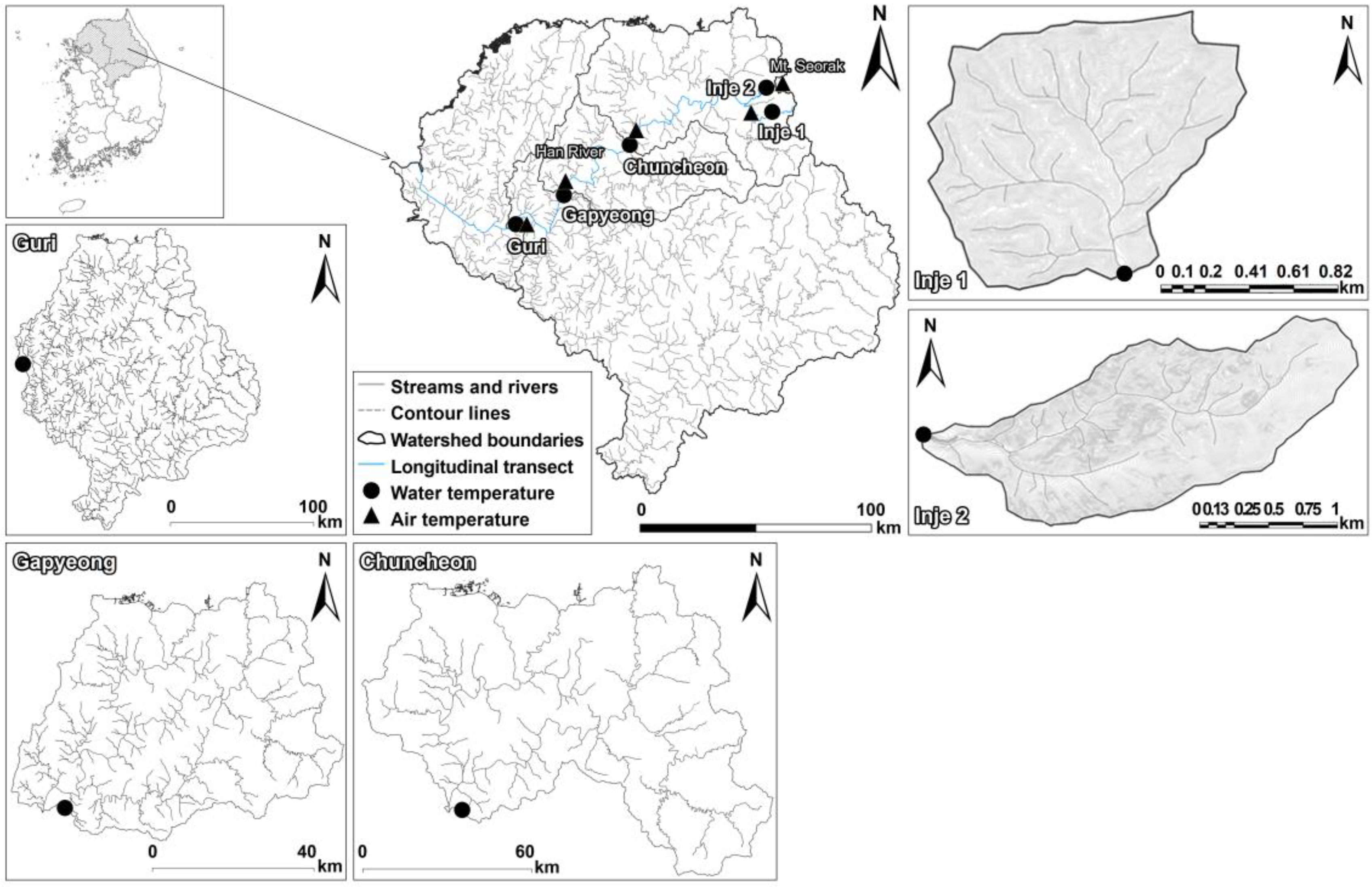
Table 1. Summary of the observed sites from upper to lower reaches.

Reach	Site	Area (km2)	Altitude (m a.s.l.)	Channel Length (km)	Channel Slope (m/m)	Canopy Cover	Distance (km)
Upper	Inje 1	1.06	490–845	1.52	0.23	Open/Close	287.4
Upper	Inje 2	1.99	580–1155	3.16	0.18	Open/Close	282.9
Middle	Chuncheon	4462.41	50–1708	137.35	0.0077	Open	167.7
Middle	Gapyeong	7149.71	40–1708	190.52	0.0054	Open	114.6
Lower	Guri	20,865.70	14–1708	233.49	0.0045	Open	71.6

Note: m a.s.l.: meters above sea level; Range from minimum to maximum values. Distance refers to longitudinal distances from the upper Han River basin in the Seorak region to each monitoring point.

Table 1. Summary of the observed sites from upper to lower reaches.

Reach	Site	Area (km2)	Altitude (m a.s.l.)	Channel Length (km)	Channel Slope (m/m)	Canopy Cover	Distance (km)
Upper	Inje 1	1.06	490–845	1.52	0.23	Open/Close	287.4
Upper	Inje 2	1.99	580–1155	3.16	0.18	Open/Close	282.9
Middle	Chuncheon	4462.41	50–1708	137.35	0.0077	Open	167.7
Middle	Gapyeong	7149.71	40–1708	190.52	0.0054	Open	114.6
Lower	Guri	20,865.70	14–1708	233.49	0.0045	Open	71.6

Note: m a.s.l.: meters above sea level; Range from minimum to maximum values. Distance refers to longitudinal distances from the upper Han River basin in the Seorak region to each monitoring point.

2.2. Field Monitoring and Data Analysis

Field monitoring was conducted from 2020 to 2025, with analyses restricted to the May–October period of each year. Monitoring was not conducted during winter or early spring (i.e., December to March) because the stream and river watersheds are frozen during this period. T_W at upper reaches was measured using capacitance water stage data loggers (OTT-Orpheus Mini Water Level Logger, OTT Messtechnik, Kempten, Germany) at 10 min intervals. T_W was monitored at 5 min intervals at middle and lower reaches using YSI EXO2 multiparameter sondes at the Chuncheon and Gapyeong sites and a YSI 6600 multiparameter sonde at the Guri site. T_W data for the three river sites were obtained from the Uiam, Gapyeong, and Guri stations of the National Institute of Environmental Research. These datasets were comparable in terms of measurement depth and temporal resolution, and consistency across sources was ensured through sensor calibration and outlier screening. T_A data were obtained from Gilin AWS in Inje 1 site, Osaeg AWS in Inje 2 site, Chuncheon ASOS in Chuncheon site, Cheongpyeong AWS in Gapyeong site, and Gangdong AWS in Guri site (Figure 1). Weather stations used for T_A monitoring were selected based on proximity to T_W measurement sites (2.7–9.7 km) and are managed by the Korea Meteorological Administration Weather Data Service.

To analyze the relationship between T_A and T_W across the upper (two forested streams), middle (two rivers), and lower (one river) reaches, hysteresis loops were constructed based on the T_A and T_W time series, following the methods used in previous studies [49,50,51]. T_A and T_W data from 2020 to 2025 were classified into warming (May–July) and cooling (August–October) phases based on previous studies of seasonal variation in T_A and T_W [50,52,53]. The air–water temperature difference (AWTD) was calculated as the difference between the daily T_A and T_W values, e.g., [54].

The temperature elasticity approach may be defined as the proportional change in T_W resulting from a change in T_A at any given time [37,55]. In reality, the term elasticity used in a previous study, which originated in economics (e.g., price elasticity of demand), was subsequently adopted by many disciplines as a measure of responsiveness [56] and has become a popular tool among empiricists because of its independent units and simplified data analysis. A well-known aspect of elasticity in hydrology is the precipitation elasticity of streamflow, which is defined as the proportional change in river flow in response to a proportional change in precipitation [38,39,40]. Thus, we designed temperature elasticity of the nonparametric estimator, e.g., [38] for T_W with respect to T_A (mean daily dataset) on the hysteresis loop (as warming and cooling phases), as follows:

$$Temperature elasticity = median\left({\displaystyle \frac{T_W - \overline{T_W}}{T_A - \overline{T_A}}} \times {\displaystyle \frac{\overline{T_A}}{\overline{T_W}}}\right)$$

(1)

where T_A and T_W denote the air and water temperatures at a given time, respectively, and $\overline{T_A}$ and $\overline{T_W}$ denote the daily mean air (T_A) and water (T_W) temperatures during the May–October observation period.

The temperature elasticity approach has some merits over other techniques, including that the whole function of temperature elasticity is characterized by its median value, which minimizes the impact of outliers (i.e., flood and drought). The median is used to minimize the impact of outliers, such as extreme events, which have the greatest effect on biota [37,57]. temperature elasticity is also dimensionless, which simplifies data analysis.

Statistical analyses were conducted via one-way analysis of variance followed by the Kruskal–Wallis test, depending on the assumptions of normality and variance equality, e.g., [58], to compare the mean differences in T_W and T_A among the five reaches during the observation period. All statistical analyses were performed using IBM SPSS Statistics 30 (IBM Corp., Armonk, NY, USA) and R version 4.1.2 (R Foundation for Statistical Computing, Vienna, Austria).

3. Results

3.1. Water Temperatures Responses to Air Temperature Changes

The daily mean T_A and T_W during the observation period ranged from 4.5 to 32.3 and 6.9 to 30.6 °C, respectively, across the upper (Inje 1 and Inje 2 sites), middle (Chuncheon and Gapyeong sites), and lower (Guri site) reaches (Figure 2a,b). T_W exhibited clear spatial variation, whereas T_A showed relatively limited spatial variation (Figure 2).

The daily mean T_A (±SD) among the five reaches was similar, ranging from 19.2 to 22.0 °C (±5.1–5.4 °C). There was a significant difference in mean T_A among the upper, middle, and lower reaches at the 99% confidence level (p < 0.001) (Table 2; Figure 2). The daily mean T_W among the five reaches was lowest in the upper reaches (14.6 ± 3.2 and 14.3 ± 2.9 °C), followed by the middle reaches (20.6 ± 3.9 and 21.0 ± 3.5 °C), and highest in the lower reaches (21.9 ± 3.7 °C) (Table 2; Figure 2). There was a significant difference in the mean T_W between the upper, middle, and lower reaches at the 99% confidence level (p < 0.001) (Figure 2b). The T_W responses in the upper reaches (Inje 1 and Inje 2 sites) were distributed over a relatively wide range, whereas those from the middle (Chuncheon and Gapyeong sites) to the lower (Guri sites) reaches exhibited a narrower range.

The mean AWTD over the 6-year period ranged from −0.6 to 5.5 °C (±3.2–3.6) °C across the upper, middle, and lower reaches, spanning longitudinal distances of 71.6 to 287.4 km from the upper Han River basin in the mountainous region to each monitoring point (Figure 3). The mean AWTDs in the two upper reaches (Inje 1 and Inje 2 sites) were 4.6 and 5.5 °C (±3.2 and 3.6 °C), whereas there was no difference between T_A and T_W in the middle or lower reaches (Figure 3). The AWTD differed significantly between the upper, middle, and lower reaches at the 99% confidence level (p < 0.001), with a significant difference also observed between the middle (Gapyeong site) and lower (Guri site) reaches.

Table 2. Summary of daily mean air and water temperatures at the five reaches.

Reach	Site	n	TA (°C)	TW (°C)	AWTD (°C)
Upper	Inje 1	1104	19.2 ± 5.3 (3.2–28.2)	14.6 ± 3.2 (6.9–20.6)	4.6 ± 3.2 (−7.6–12.9)
Upper	Inje 2	1098	19.8 ± 5.1 (4.7–30.0)	14.3 ± 2.9 (7.7–19.0)	5.5 ± 3.6 (−5.4–14.6)
Middle	Chuncheon	1019	21.1 ± 5.4 (5.0–30.2)	20.6 ± 3.9 (11.7–30.6)	0.5 ± 3.4 (−13.6–9.3)
Middle	Gapyeong	1010	20.4 ± 5.2 (4.5–32.3)	21.0 ± 3.5 (13.8–30.0)	−0.6 ± 3.3 (−14.2–8.8)
Lower	Guri	930	22.0 ± 5.2 (6.5–31.4)	21.9 ± 3.7 (14.8–30.2)	0.05 ± 3.3 (−13.4–11.4)

Note: T_A: air temperature; T_W: water temperature; AWTD: air–water temperature difference; n: number observed days. Mean ± standard deviation (SD). Bracket: minimum–maximum values.

Table 2. Summary of daily mean air and water temperatures at the five reaches.

Reach	Site	n	TA (°C)	TW (°C)	AWTD (°C)
Upper	Inje 1	1104	19.2 ± 5.3 (3.2–28.2)	14.6 ± 3.2 (6.9–20.6)	4.6 ± 3.2 (−7.6–12.9)
Upper	Inje 2	1098	19.8 ± 5.1 (4.7–30.0)	14.3 ± 2.9 (7.7–19.0)	5.5 ± 3.6 (−5.4–14.6)
Middle	Chuncheon	1019	21.1 ± 5.4 (5.0–30.2)	20.6 ± 3.9 (11.7–30.6)	0.5 ± 3.4 (−13.6–9.3)
Middle	Gapyeong	1010	20.4 ± 5.2 (4.5–32.3)	21.0 ± 3.5 (13.8–30.0)	−0.6 ± 3.3 (−14.2–8.8)
Lower	Guri	930	22.0 ± 5.2 (6.5–31.4)	21.9 ± 3.7 (14.8–30.2)	0.05 ± 3.3 (−13.4–11.4)

Note: T_A: air temperature; T_W: water temperature; AWTD: air–water temperature difference; n: number observed days. Mean ± standard deviation (SD). Bracket: minimum–maximum values.

Figure 2. Box plots of (a) daily mean air (T_A) and (b) water (T_W) temperature at all sites during the observation period. The upper and lower hinges represent the first and third quartiles, respectively (25th and 75th percentiles, respectively). Whiskers extend to 1.5 times the interquartile range, and data points beyond the whiskers represent outliers. Different letters (a, b, c, and d) denote statistically significant differences among periods (p < 0.001).

Figure 2. Box plots of (a) daily mean air (T_A) and (b) water (T_W) temperature at all sites during the observation period. The upper and lower hinges represent the first and third quartiles, respectively (25th and 75th percentiles, respectively). Whiskers extend to 1.5 times the interquartile range, and data points beyond the whiskers represent outliers. Different letters (a, b, c, and d) denote statistically significant differences among periods (p < 0.001).

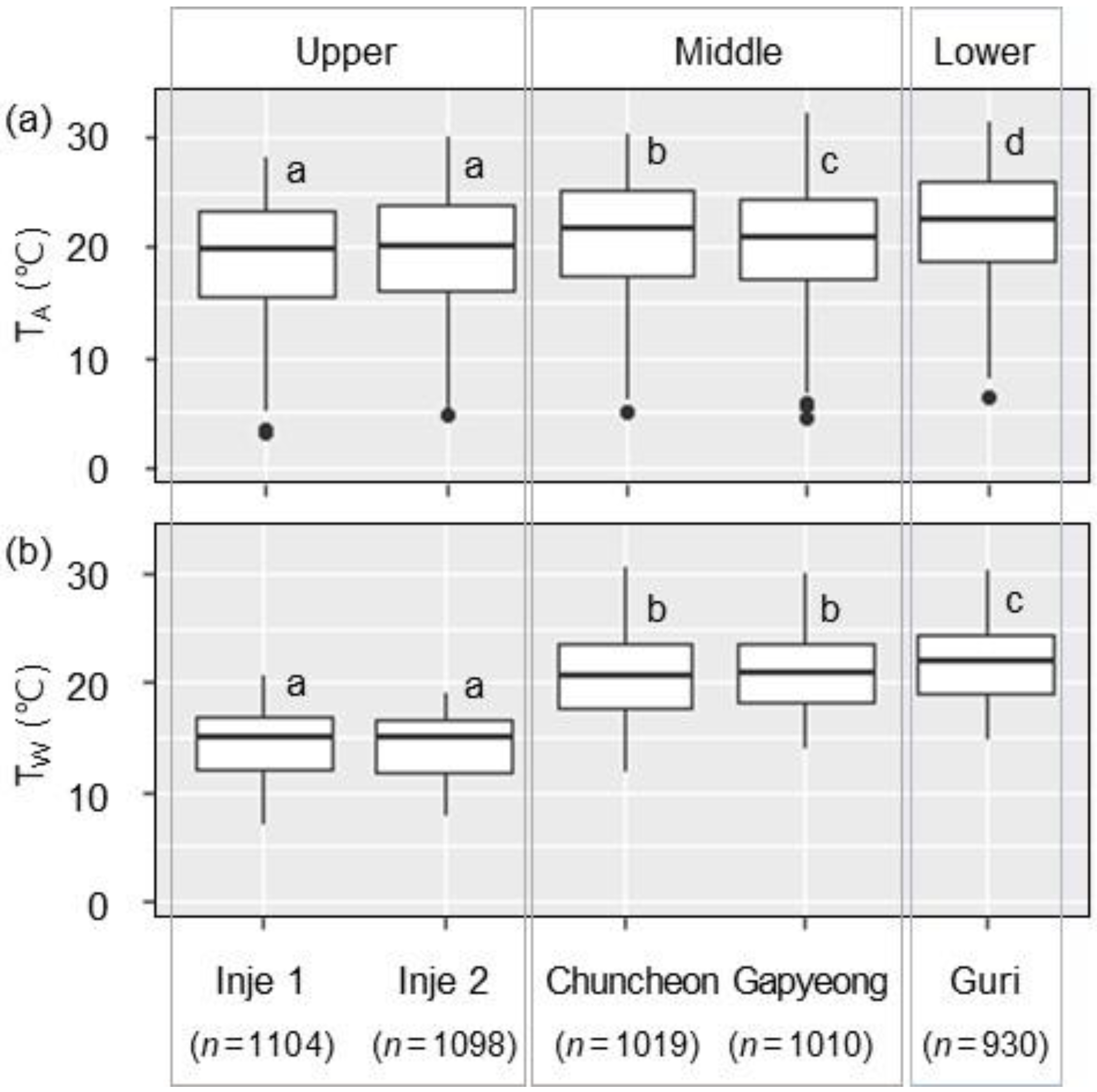
Figure 3. Maximum (◆), minimum (▲), and mean (◯) values for air–water temperature difference (AWTD; T_A–T_W) in upper (Inje 1 and Inje 2 sites), middle (Chuncheon and Gapyeong sites) and lower (Guri site) reaches from the upper Han River basin in the Seorak region to each monitoring point.

Figure 3. Maximum (◆), minimum (▲), and mean (◯) values for air–water temperature difference (AWTD; T_A–T_W) in upper (Inje 1 and Inje 2 sites), middle (Chuncheon and Gapyeong sites) and lower (Guri site) reaches from the upper Han River basin in the Seorak region to each monitoring point.

3.2. Hysteresis Loop Analysis Between Air and Water Temperatures

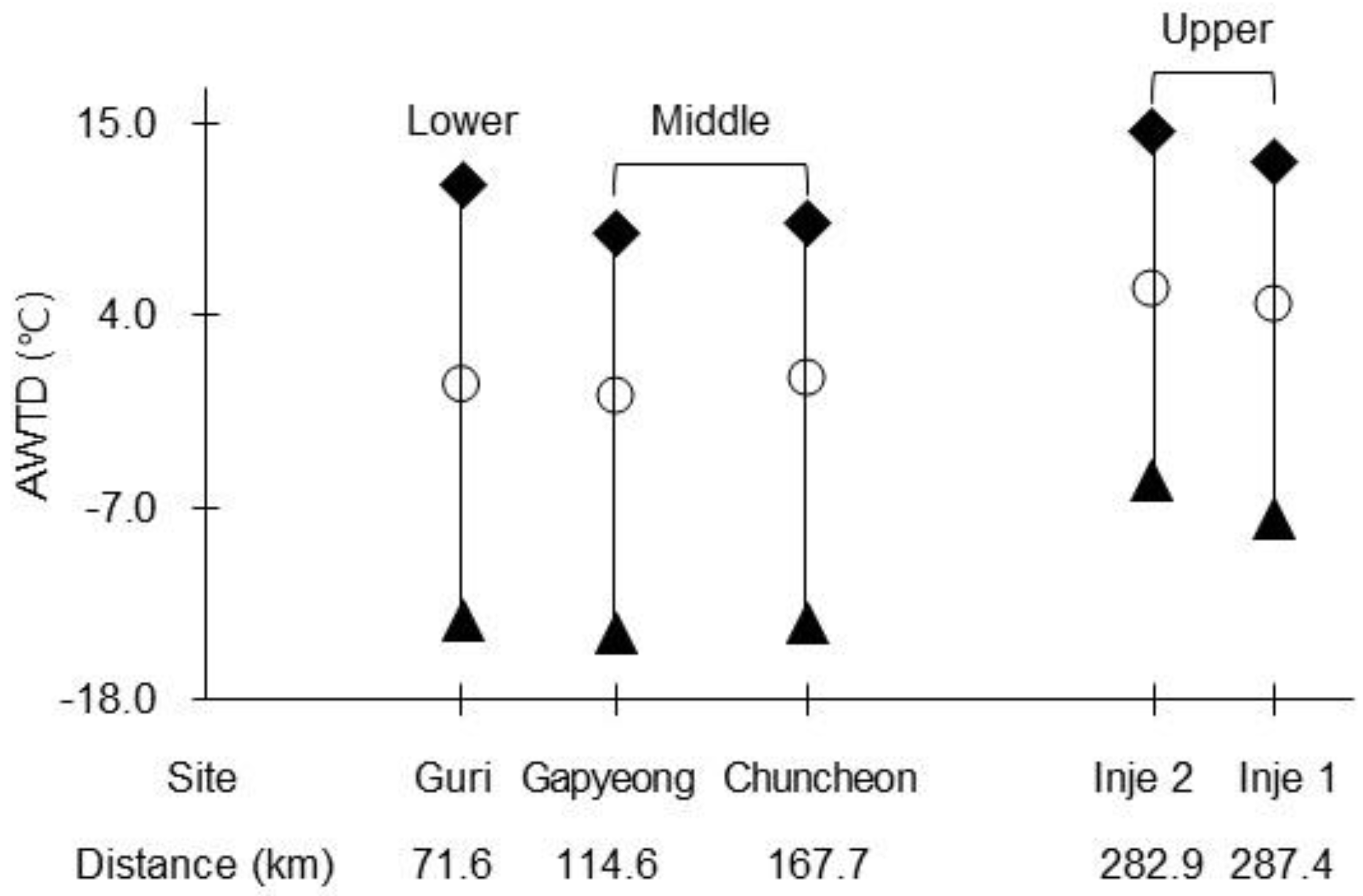
The T_W changes in response to T_A variations formed distinct curve shapes, indicating a hysteresis loop between T_A and T_W. From the hysteretic loops, the relationship between T_A and T_W was analyzed by separating the observation period (excluding winter) into warming (May–July) and cooling (August–October) phases (Figure 4). As shown in Figure 4a–e, in the upper reaches (Inje 1 and Inje 2 sites), T_W exhibited a lower temperature response than T_A during the warming phase, whereas T_W and T_A exhibited similar responses during the cooling phase (Figure 4f–i). Compared with the middle and lower reaches (Chuncheon, Gapyeong, and Guri sites), the upper reaches (Inje 1 and Inje 2) showed a greater T_A–T_W difference during the warming phase (approximately 4–5 °C), while the difference became smaller during the cooling phase (approximately 4–6 °C) (Figure 4).

The relationships between T_A and T_W were strong (R² values of 0.52–0.88) and were significant at all sites in both periods (p < 0.001) (Figure 4, Table 3). Because the analysis is based on daily time series data, some degree of autocorrelation may be present, potentially affecting the magnitude of statistical metrics such as the F-values reported in Table 3. However, given the large sample size and the consistency of patterns across sites, the overall relationships are considered robust. The regression slopes showed distinct temporal and spatial variations in thermal sensitivity (Table 3). In both phases, T_W increased with increasing T_A, exhibiting a linear relationship. However, the slope during the warming phase (0.428–0.722) was steeper than that during the cooling phase (0.459–0.620) (Table 3). A comparison of the five reaches showed that the slope in the middle reaches was the steepest in the warming phase (0.722 and 0.661, respectively), whereas the slopes became similar across all reaches during the cooling phase (0.459–0.620). Moreover, the upper reaches showed the lowest slopes (0.428–0.520) during both phases (Table 3). As shown in Figure 4a–j, the maximum correlation between T_A and T_W differed between the two phases, with correlation coefficients ranging from 0.724 to 0.936 across all sites (p < 0.001). T_A and T_W were most strongly correlated with the cooling phase, with a correlation coefficient of 0.936 (p < 0.001) for a site in the upper reach (Inje 1 site) and 0.909 (p < 0.001) for the site in the lower reach (Guri site) (Figure 4f,j).

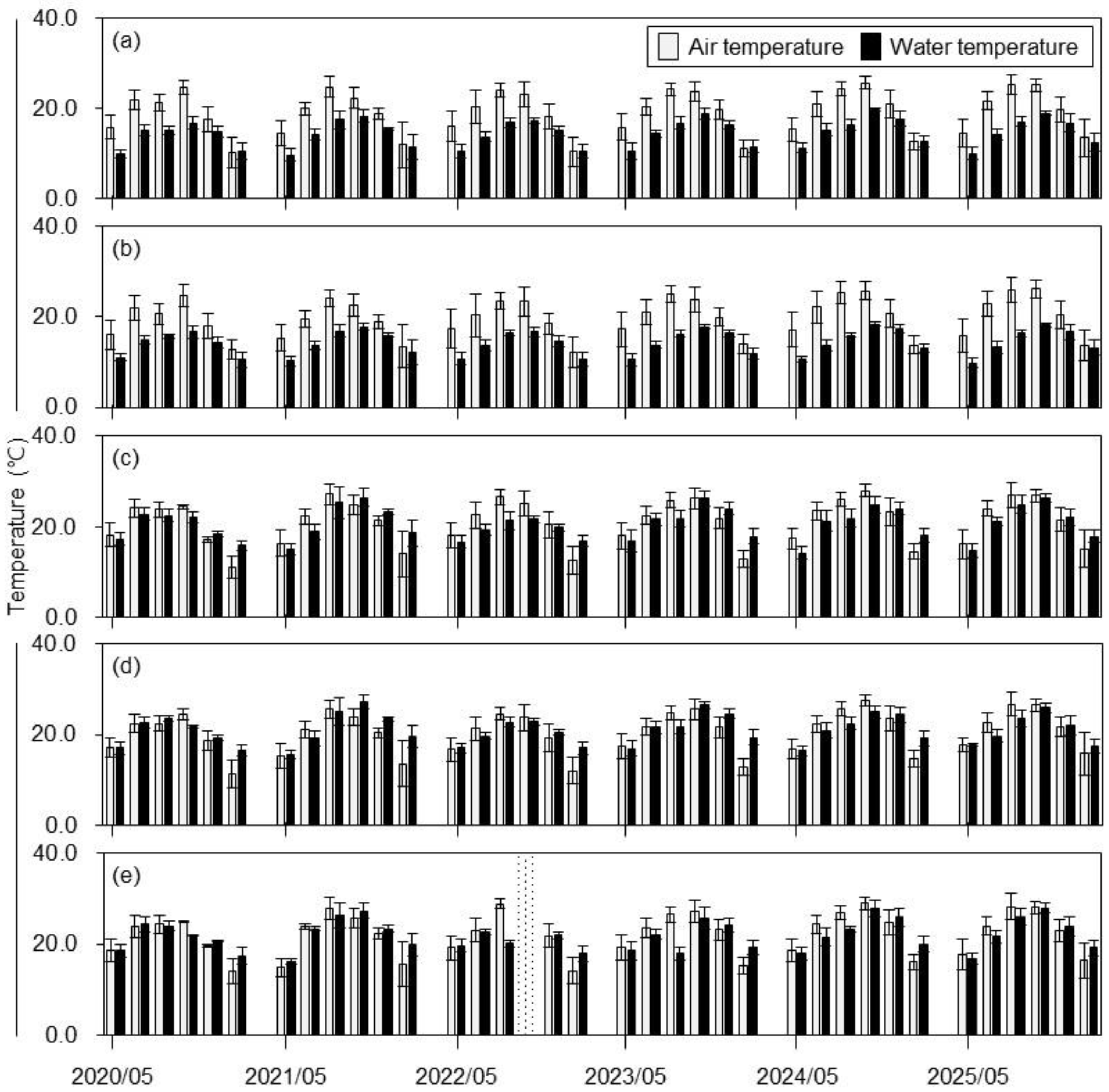
Regarding the relationship between monthly mean T_A and T_W (i.e., its primary controlling factor), T_A, the minimum and maximum fluctuations in T_A exhibited similar patterns between the two phases across all five reaches. In contrast, T_W showed larger minimum and maximum fluctuations during the warming phase than during the cooling phase (Figure 5a–e). The five reaches exhibited relatively narrow ranges of minimum and maximum T_W fluctuations (approximately 6–7 °C) in both phases. Notably, phases-dependent differences in T_W fluctuations were not pronounced in middle and lower reaches (Chuncheon, Gapyeong, and Guri sites) (Figure 5c,d). In contrast, the upper reaches (Inje 1 and Inje 2 sites) showed a distinct reach-dependent pattern, with T_W fluctuations during the warming phase occurring at lower temperature ranges than those during the cooling phase, indicating a clear hysteretic response (Figure 5a,b).

Table 3. Summary of the regression analyses for daily mean air and water temperatures.

Phase	Reach	Site	Slope (a)	95% CI (a)	Intercept (b)	95% CI (b)	R2	n	F	p
Warming	Upper	Inje 1	0.595	0.569–0.621	1.876	1.342–2.411	0.79	552	2016.73	<0.001
	Upper	Inje 2	0.428	0.396–0.460	4.696	4.024–5.367	0.56	549	697.22	<0.001
	Middle	Chuncheon	0.722	0.682–0.762	3.837	2.936–4.738	0.71	524	1257.95	<0.001
	Middle	Gapyeong	0.661	0.624–0.699	6.138	5.328–6.949	0.71	500	1209.73	<0.001
	Lower	Guri	0.557	0.509–0.606	8.419	7.293–9.544	0.52	466	512.32	<0.001
Cooling	Upper	Inje 1	0.520	0.504–0.536	5.795	5.481–6.110	0.88	552	3906.14	<0.001
	Upper	Inje 2	0.459	0.437–0.481	6.372	5.941–6.804	0.76	549	1711.61	<0.001
	Middle	Chuncheon	0.556	0.530–0.581	10.354	9.822–10.886	0.79	495	1834.50	<0.001
	Middle	Gapyeong	0.537	0.510–0.564	11.261	10.706–11.817	0.75	510	1504.78	<0.001
	Lower	Guri	0.620	0.594–0.646	9.642	9.073–10.211	0.83	464	2192.29	<0.001

Note: Equation: T_W = aT_A + b; CI: confidence interval; n: number of observed days. Values range from minimum to maximum.

Table 3. Summary of the regression analyses for daily mean air and water temperatures.

Phase	Reach	Site	Slope (a)	95% CI (a)	Intercept (b)	95% CI (b)	R2	n	F	p
Warming	Upper	Inje 1	0.595	0.569–0.621	1.876	1.342–2.411	0.79	552	2016.73	<0.001
	Upper	Inje 2	0.428	0.396–0.460	4.696	4.024–5.367	0.56	549	697.22	<0.001
	Middle	Chuncheon	0.722	0.682–0.762	3.837	2.936–4.738	0.71	524	1257.95	<0.001
	Middle	Gapyeong	0.661	0.624–0.699	6.138	5.328–6.949	0.71	500	1209.73	<0.001
	Lower	Guri	0.557	0.509–0.606	8.419	7.293–9.544	0.52	466	512.32	<0.001
Cooling	Upper	Inje 1	0.520	0.504–0.536	5.795	5.481–6.110	0.88	552	3906.14	<0.001
	Upper	Inje 2	0.459	0.437–0.481	6.372	5.941–6.804	0.76	549	1711.61	<0.001
	Middle	Chuncheon	0.556	0.530–0.581	10.354	9.822–10.886	0.79	495	1834.50	<0.001
	Middle	Gapyeong	0.537	0.510–0.564	11.261	10.706–11.817	0.75	510	1504.78	<0.001
	Lower	Guri	0.620	0.594–0.646	9.642	9.073–10.211	0.83	464	2192.29	<0.001

Note: Equation: T_W = aT_A + b; CI: confidence interval; n: number of observed days. Values range from minimum to maximum.

Figure 4. Relationships between daily mean air (T_A) and water (T_W) temperatures determined by the hysteresis loop: (a–e) warming and (f–j) cooling phases in upper (Inje 1 and Inje 2 sites) and middle (Chuncheon and Gapyeong sites), and lower (Guri site) reaches during each observation period. Thick lines represent linear fits estimated by regression analysis for the hysteresis loop. r and p values indicate the correlation coefficient and significance, respectively.

Figure 4. Relationships between daily mean air (T_A) and water (T_W) temperatures determined by the hysteresis loop: (a–e) warming and (f–j) cooling phases in upper (Inje 1 and Inje 2 sites) and middle (Chuncheon and Gapyeong sites), and lower (Guri site) reaches during each observation period. Thick lines represent linear fits estimated by regression analysis for the hysteresis loop. r and p values indicate the correlation coefficient and significance, respectively.

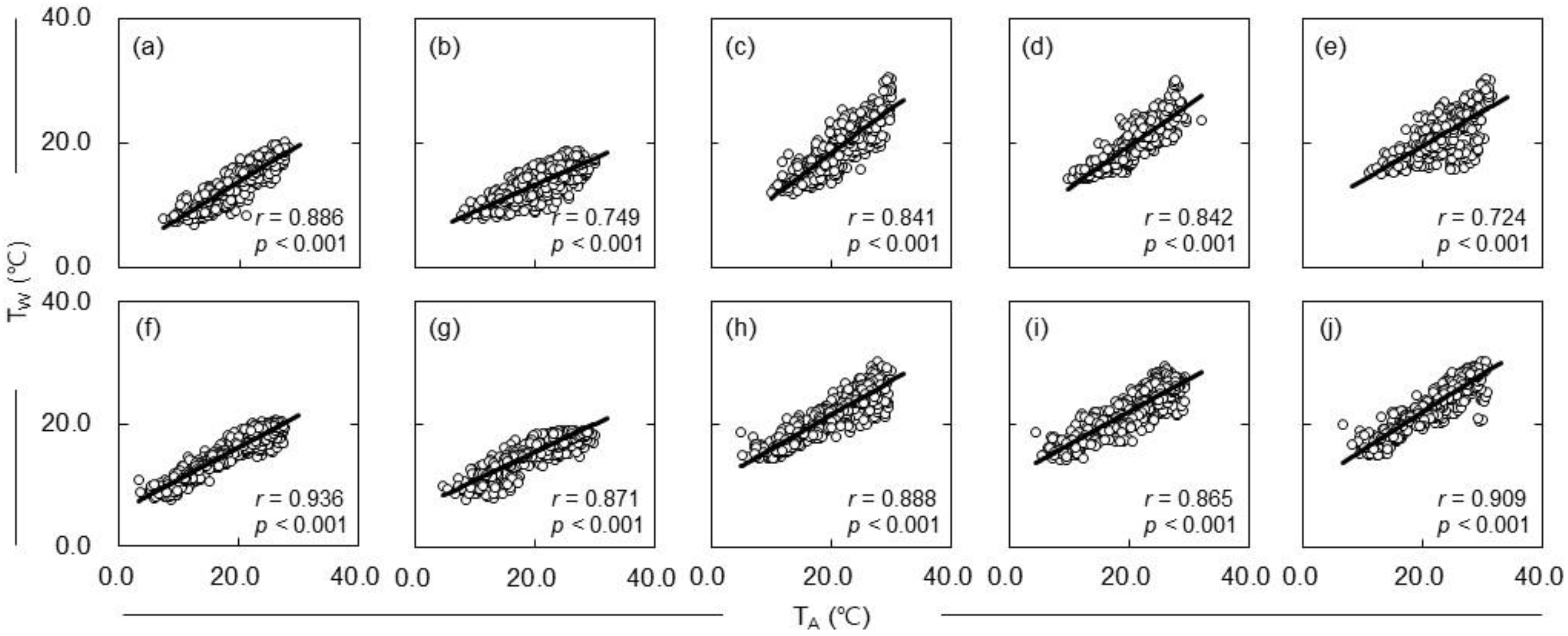
Figure 5. Monthly mean air (T_A) and water (T_W) temperatures showing the range between maximum and minimum values at five sites: (a,b) upper (Inje 1 and Inje 2 sites), (c,d) middle (Chuncheon and Gapyeong sites), and (e) lower (Guri site) reaches. The dotted area indicates no data.

Figure 5. Monthly mean air (T_A) and water (T_W) temperatures showing the range between maximum and minimum values at five sites: (a,b) upper (Inje 1 and Inje 2 sites), (c,d) middle (Chuncheon and Gapyeong sites), and (e) lower (Guri site) reaches. The dotted area indicates no data.

3.3. Approach of Temperature Elasticity on the Hysteresis Loop

For spatial interpretation along the longitudinal gradient, the five monitoring sites were grouped into three reaches: upper, middle, and lower reaches. The temperature elasticity was then calculated for each of the three reaches using monthly observations during the study period (Figure 6). Temperature elasticity value across the three reaches ranged from −0.940 to 1.814 over the 36-month observation period. The temperature elasticity values were predominantly positive across all three reaches; however, those in the middle and lower reaches tended to be lower than those in the upper reaches, and occasionally exhibited negative excursions (Figure 6a–c). Negative temperature elasticity values were occasionally observed, indicating a temporary decoupling between T_A and T_W.

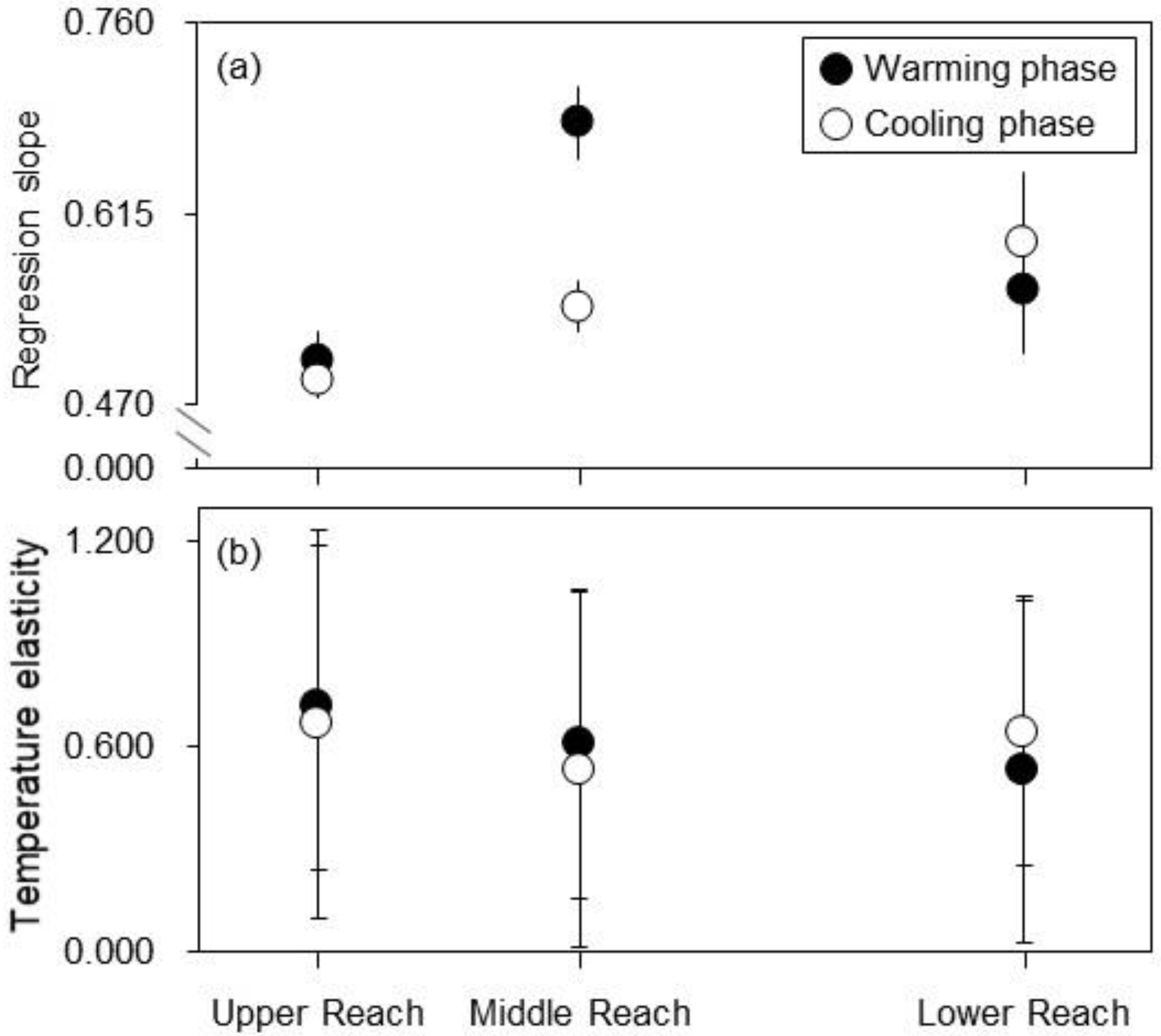
Spatial changes in T_W responses to T_A from upper to the lower reaches showed opposite patterns, separated into two different phases (Table 4; Figure 7). The regression slope increased toward the lower reach, whereas the temperature elasticity decreased, with the most pronounced changes observed in the slope during the cooling phase (0.489–0.620) and the temperature elasticity during the warming phase (0.714–0.532).

Under these conditions, the regression slope was steepest in the Middle Reach (0.684) of the warming phase and in the lower reach (0.620) of the cooling phase (Table 4; Figure 7a). The regression slope during the warming phase increased from the upper to the middle reaches and slightly decreased toward the lower reach (0.505–0.557), in particular the regression slope of the cooling phase increased progressively from the upper to lower reaches (0.489–0.545) (Figure 7a). From the hysteresis loops, the mean temperature elasticity (±SD) was 0.532–0.714 (±0.452–0.507) and 0.533–0.667 (±0.388–0.567) in the warming and cooling phases, respectively (Table 4; Figure 7b). The temperature elasticity showed relatively small spatial differences among the reaches (Figure 7b). Here, during the warming phase, the temperature elasticity decreased from the upper to the lower reaches (0.714–0.532), besides the temperature elasticity decreased from the upper to the middle reaches and slightly increased toward the lower reach (0.667–0.641) (Figure 7b).

Figure 6. Temperature elasticity in (a) upper (Inje 1 and Inje 2 sites), (b) middle (Chuncheon and Gapyeong sites), and (c) lower (Guri site) reaches during the warming and cooling phases throughout the observation period. The horizontal dashed lines indicate the mean temperature elasticity value. The dotted area indicates no data.

Figure 6. Temperature elasticity in (a) upper (Inje 1 and Inje 2 sites), (b) middle (Chuncheon and Gapyeong sites), and (c) lower (Guri site) reaches during the warming and cooling phases throughout the observation period. The horizontal dashed lines indicate the mean temperature elasticity value. The dotted area indicates no data.

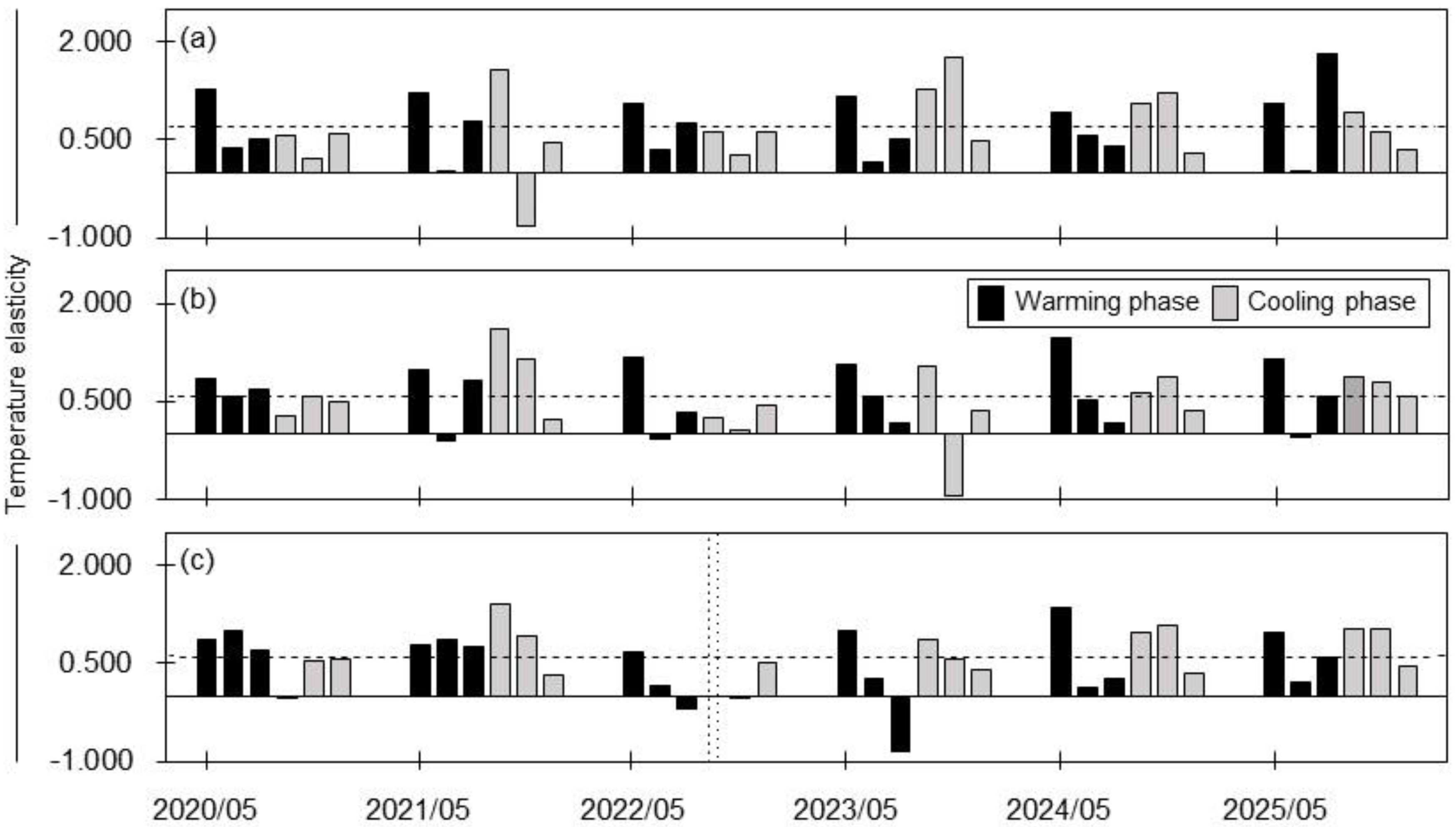
Table 4. Distribution of regression slope and temperature elasticity across the upper, middle, and lower reaches during warming and cooling phases.

Phase	Reach	Site	Slope (a)	95% CI	Temperature Elasticity
Warming	Upper	Inje 1—Inje 2	0.505	0.483–0.526	0.714 ± 0.472 (0.004–1.814)
	Middle	Chuncheon—Gapyeong	0.684	0.656–0.712	0.605 ± 0.452 (−0.107–1.480)
	Lower	Guri	0.557	0.509–0.606	0.532 ± 0.507 (−0.837–1.348)
Cooling	Upper	Inje 1—Inje 2	0.489	0.475–0.503	0.667 ± 0.567 (−0.819–1.771)
	Middle	Chuncheon—Gapyeong	0.545	0.526–0.564	0.533 ± 0.517 (−0.940–1.614)
	Lower	Guri	0.620	0.594–0.646	0.641 ± 0.388 (−0.035–1.413)

Note: CI: confidence interval; Mean ± standard deviation. Bracket: minimum–maximum values.

Table 4. Distribution of regression slope and temperature elasticity across the upper, middle, and lower reaches during warming and cooling phases.

Phase	Reach	Site	Slope (a)	95% CI	Temperature Elasticity
Warming	Upper	Inje 1—Inje 2	0.505	0.483–0.526	0.714 ± 0.472 (0.004–1.814)
	Middle	Chuncheon—Gapyeong	0.684	0.656–0.712	0.605 ± 0.452 (−0.107–1.480)
	Lower	Guri	0.557	0.509–0.606	0.532 ± 0.507 (−0.837–1.348)
Cooling	Upper	Inje 1—Inje 2	0.489	0.475–0.503	0.667 ± 0.567 (−0.819–1.771)
	Middle	Chuncheon—Gapyeong	0.545	0.526–0.564	0.533 ± 0.517 (−0.940–1.614)
	Lower	Guri	0.620	0.594–0.646	0.641 ± 0.388 (−0.035–1.413)

Note: CI: confidence interval; Mean ± standard deviation. Bracket: minimum–maximum values.

Figure 7. Relationships between the warming and cooling phases for: (a) the regression slope; and (b) temperature elasticity across the upper, middle, and lower reaches of the watershed. Error bars show the 95% confidence intervals for the regression slopes in (a) and the standard deviation for temperature elasticity in (b).

Figure 7. Relationships between the warming and cooling phases for: (a) the regression slope; and (b) temperature elasticity across the upper, middle, and lower reaches of the watershed. Error bars show the 95% confidence intervals for the regression slopes in (a) and the standard deviation for temperature elasticity in (b).

4. Discussion

4.1. Temporal Characteristics of Water Temperature Responses to Air Temperature

In the streams (upper reach) and the rivers (middle and lower reaches), increases in T_A were consistently associated with increases in T_W. However, the magnitude of T_W variation was smaller than that of T_A variation, which may be attributed to the higher specific heat capacity of water than that of air [19,59]. Regarding the response of T_W to T_A changes, Moore et al. [3] reported that an increase in T_A led to an increase in mean T_W of up to approximately 1.4 °C in a catchment in British Columbia. Similarly, Lane et al. [21] found that T_W increased when T_A exceeded 30 °C and decreased when T_A dropped below 12 °C at the mouth of the Mississippi River. In addition, monsoon-driven hydroclimatic responses have been reported in East Asia; for example, in the Nakdong River basin, Park et al. [60] observed that mean T_W increased by 0.2–0.7 °C in June, when T_A was increasing, and decreased by 0.2–1.1 °C in September, when T_A was decreasing. Yu et al. [61] reported that monthly mean T_W exhibited a weaker increasing trend than T_A, with greater increases in August than in July and a continued increase into September in Lake Paldang. Cui et al. [62] also showed that surface T_W exhibited hysteresis behavior in relation to T_A in the Poyang Lake.

The response of T_W to T_A was more pronounced during the T_A-increasing period (May–July) than during the T_A-decreasing period (August–October). This pattern reflects the characteristic seasonal variation in T_W in the ROK, where T_A increases from spring to early summer and decreases from late summer to autumn. In summer, the water surface undergoes experiences greater latent heat loss through evaporation than in winter, and the contributions of groundwater inflow or snowmelt to streamflow also vary seasonally [6,14]. Consequently, during the T_A-increasing phase, T_W tended to increase from a relatively low baseline, whereas during the T_A-decreasing phase, elevated T_W was maintained for a certain period before decreasing, reflecting thermal inertia [53,60]. Similarly, An and Lee [51] reported a delayed T_W response relative to changes in T_A, manifested as a hysteresis loop, which they attributed to the higher specific heat capacity of water than of air.

To analyze the response of T_W to temporal variations in T_A, hysteresis loop analysis was applied, in which T_W followed different trajectories during the increasing and decreasing phases of T_A (Figure 4 and Figure 5). Additionally, the correlation between TA and TW was stronger during the cooling phase. This stronger correlation likely reflects increased thermal inertia and delayed heat exchange between air and water. Because the rates of increase and decrease in T_W differed between the warming and cooling phases of T_A [52], the slope during the warming phase (0.428–0.722) was steeper than that during the cooling phase (0.459–0.620). In contrast, the coefficient of determination (R²) was higher during the cooling phase (0.75–0.88) than during the warming phase (0.52–0.79). Similar patterns were reported by Nam et al. [27], who found that the slope of the linear relationship between T_A and T_W was slightly steeper during summer (0.763) than during the fall season (0.736); whereas the R² value was higher during the fall (0.834).

4.2. Relative Influence of Spatial Distribution on Water Temperature from Stream to River

The principal component representing the temporal characteristics of T_W exhibited a response pattern similar to that of T_A. However, the indicator describing T_W variability, namely AWTD, showed either lower or higher values in the streams (upper reaches) than in the rivers (middle and lower reaches). Here, canopy cover and topographic characteristics, including altitude, channel length, channel slope, and longitudinal position, were quantified using site-specific data (Table 1). However, groundwater influence and drainage winds were not directly measured and therefore are discussed only as potential explanatory factors based on site characteristics. From the site characteristics, this difference may be attributed to the relatively high elevation of the streams (upper reaches; 490–1155 m a.s.l.) and to variations in riparian forest cover and understory vegetation conditions along the streamside, which range from open to closed canopies (Table 1). These factors regulate the amount of solar radiation reaching the water surface through differences in canopy shading [2,10,63,64]. Additionally, spatial heterogeneity in topography between the streams (upper reaches) and the rivers (middle and lower reaches) likely altered flow paths and channel hydraulics, thereby contributing to differences in the extent to which controlling factors influenced T_W responses [65,66].

In this study, although the responses of T_W to T_A exhibited similar overall patterns across the two phases, distinct differences were observed between reaches. During the warming phase, T_W in the streams (upper reaches) remained consistently lower than T_A, whereas in the cooling phase, T_W in the rivers (middle and lower reaches) remained higher than T_A (Figure 2, Figure 3 and Figure 4). For the lowland rivers in the middle and lower reaches, this pattern is consistent with previous studies attributing such behavior to differences in heat capacity between T_A and T_W, e.g., [7,51,59]. In contrast, the streams in the present study are adjacent to steep hillslopes and are strongly influenced by shaded riparian zones, which provide solar-radiation blocking as well as cooling and humidifying effects. Consequently, T_W variation in response to T_A changes was greater in streams than in rivers, leading to a larger difference between T_A and T_W during the warming phase, particularly in summer, e.g., [52,67]. Moreover, because the study sites are streams constrained by steep side slopes, the riparian zone may be narrow or poorly developed, e.g., [68,69]. Thus, in the streams examined in the present study, the combined effects of a narrow riparian zone and adjacent steep side slopes led temporal variations in the difference between minimum and maximum T_W that differed markedly from those in the rivers (Figure 5 and Figure 7).

A similar pattern was evident in temperature elasticity, which characterizes the T_W response to T_A, along the longitudinal continuum from the streams (upper reaches) to the two river reaches (middle and lower reaches) in the Han River basin. Shon et al. [70] also reported that temperature elasticity increased from the upper to lower reaches in the Nakdong River watershed, primarily because of the combined effects of flow velocity and water surface area. Consistent with Shon et al. [70], higher temperature elasticity values were observed in the upper reaches than in the middle and lower reaches. These geomorphic characteristics may reduce flow velocity, thereby enhancing the sensitivity of T_W to T_A variability. However, the streams (upper reaches) within the forested watershed differ from the rivers (middle and lower reaches) in terms of channel length (1.52 and 3.16 km, respectively) and slope (0.23 and 0.18 m/m, respectively) (Table 1). These geomorphic contrasts, together with hydrologic conditions in the riparian zone, likely influenced the magnitude of temperature elasticity, e.g., [20]. Moreover, only one site represented the lower reach in this study, reflecting the available monitoring configuration along the Han River continuum. Thus, the results should be interpreted as indicating relative longitudinal patterns rather than being fully representative of lower reach conditions. Temperature elasticity represents the sensitivity of T_W to changes in T_A [37,57]. Higher temperature elasticity indicates a stronger response to atmospheric forcing and limited thermal buffering capacity, whereas lower temperature elasticity reflects greater resistance to T_A changes due to buffering processes such as groundwater inflow, channel morphology, and riparian shading [71]. In addition, variations in temperature elasticity may reflect differences in forest structure and composition, which can influence the capacity of stream systems to adapt to changing climatic conditions [72].

Streams located in the upper parts of the catchments generally have relatively low flow rates and may be ephemeral compared with rivers and lakes in the lower catchment [34,35]. Additionally, summer (mid-June to mid-September), which accounts for 90% of the total rainfall, coincides largely with the East Asian monsoon (late June to mid-September) and typhoon season (late July to mid-September) in the ROK [73,74,75]. Therefore, because winter months were excluded due to freezing conditions and the absence of measurable flow, T_W, T_A, and elasticity values may be slightly overestimated and should be interpreted as representative of the non-freezing period rather than the full annual cycle. The phase boundaries were defined based on observed seasonal temperature patterns, and the results should be interpreted within this seasonal framework.

Therefore, the observed changes in T_W may be attributed largely to variations in T_A within the forested ecosystem under the hydrological conditions of the present study. For example, Kelleher et al. [71] noted that linear regression between T_A and T_W can be used to indicate general T_A–T_W sensitivity, with T_A used as a surrogate for all the cumulative atmospheric controls on T_W. Similarly, Beaufort et al. [7] explained that thermal sensitivity reflects the cumulative buffering effects of landscape characteristics on T_W. Consistent with this perspective, Ptak et al. [76] reported that, in the context of global climate change, increasing attention has been directed toward long-term variations in stream thermal regimes in forested catchments, with T_A acting as a dominant controlling factor. These variations in thermal sensitivity may have ecological implications, as changes in T_W can alter aquatic habitat conditions [77,78] and impose thermal stress on fish communities [79], although these effects were not directly examined in the present study. From a management perspective, the higher thermal sensitivity of upper reaches during the warming phase suggests that these areas should be prioritized for targeted mitigation under climate warming. Because this study was based on field observations, some missing data led to unequal sample sizes across sites and periods, and complete temporal pairing was not always possible. Therefore, the results should be interpreted primarily in terms of overall spatial and seasonal patterns rather than exact one-to-one comparisons.

5. Summary and Conclusions

The characteristics of air and water temperatures were investigated in streams and rivers of the Han River basin from 2020 to 2025, with analyses restricted to the May–October period. Using hysteresis loop analysis, we identified clear phase-dependent differences in the relationships between air and water temperatures during the warming and cooling phases. The main findings were as follows: (1) the air–water temperature difference was statistically significant across all monitored reaches during both phases (p < 0.001); (2) water temperature increased linearly with air temperature during both phases, with steeper regression slopes during the warming phase (0.428–0.722) than in the cooling phase (0.459–0.620); (3) longitudinal patterns of water temperature responses to air temperature differed between two phases; (4) the regression slopes during the cooling phase increased from the upper to the lower reaches (0.489–0.545); and (5) temperature elasticity during the warming phase decreased from the upper to the lower reaches (0.714–0.532). Overall, these results demonstrate that water temperature responses to air temperature exhibit clear phase-dependent spatial patterns, with the regression slopes varying across streams and rivers and temperature elasticity decreasing from streams to rivers. Thermal sensitivity was greater in streams, particularly during the warming phase, and diminished during the cooling phase. This study is limited by restricted site coverage and the lack of direct measurements of key controlling factors, such as groundwater inputs and riparian shading, which should be addressed in future studies. The elasticity framework could also be integrated into real-time water quality management systems to support adaptive management of stream thermal regimes under climate change.

References

- Caissie, D. The thermal regime of rivers: A review. Freshw. Biol. 2006, 51, 1389–1406. [Google Scholar] [CrossRef] [Scilit]
- Webb, B.W.; Hannah, D.M.; Moore, R.D.; Brown, L.E.; Nobilis, F. Recent advances in stream and river temperature research. Hydrol. Process. 2008, 22, 902–918. [Google Scholar] [CrossRef] [Scilit]
- Moore, R.D. Stream temperature patterns in British Columbia, Canada, based on routine spot measurements. Can. Water Resour. J. 2006, 31, 41–56. [Google Scholar] [CrossRef] [Scilit]
- Hare, D.K.; Benz, S.A.; Kurylyk, B.L.; Johnson, Z.C.; Terry, N.C.; Helton, A.M. Paired air and stream temperature analysis (PASTA) to evaluate groundwater influence on streams. Water Resour. Res. 2023, 59, e2022WR033912. [Google Scholar] [CrossRef] [Scilit]
- Assel, R.; Cronk, K.; Norton, D. Recent trends in Laurentian Great Lakes ice cover. Clim. Change 2023, 57, 185–204. [Google Scholar] [CrossRef] [Scilit]
- Stefan, H.G.; Preud’homme, E.B. Stream temperature estimation from air temperature. J. Am. Water Resour. Assoc. 1993, 29, 27–45. [Google Scholar] [CrossRef] [Scilit]
- Beaufort, A.; Moatar, F.; Sauquet, E.; Loicq, P.; Hannah, D.M. Influence of landscape and hydrological factors on stream–air temperature relationships at regional scale. Hydrol. Process. 2020, 34, 583–597. [Google Scholar] [CrossRef] [Scilit]
- Arismendi, I.; Johnson, S.L.; Dunham, J.B.; Haggerty, R. Descriptors of natural thermal regimes in streams and their responsiveness to change in the Pacific Northwest of North America. Freshw. Biol. 2013, 58, 880–894. [Google Scholar] [CrossRef] [Scilit]
- Fullerton, A.H.; Torgersen, C.E.; Lawler, J.J.; Faux, R.N.; Steel, E.A.; Beechie, T.J.; Ebersole, J.L.; Leibowitz, S.G. Rethinking the longitudinal stream temperature paradigm: Region-wide comparison of thermal infrared imagery reveals unexpected complexity of river temperatures. Hydrol. Process. 2015, 29, 4719–4737. [Google Scholar] [CrossRef] [Scilit]
- Steel, E.A.; Sowder, C.; Peterson, E.E. Spatial and temporal variation of water temperature regimes on the Snoqualmie River network. J. Am. Water Resour. Assoc. 2016, 52, 769–787. [Google Scholar] [CrossRef] [Scilit]
- Benda, L.; Miller, D.; Dunne, T.; Poff, L.; Reeves, G.; Pollock, M.; Pess, G. Network dynamics hypothesis: Spatial and temporal organization of physical heterogeneity in rivers. Bioscience 2004, 54, 413–427. [Google Scholar] [CrossRef] [Scilit]
- Rivers-Moore, N.A.; Jewitt, G.P.W. Adaptive management and water temperature variability within a South Africa river system: What are the management options? J. Environ. Manag. 2007, 82, 39–50. [Google Scholar] [CrossRef] [Scilit]
- Alcamo, J.; Vörösmarty, C.; Naiman, R.J.; Lettenmaier, D.; Pahl-Wostl, C. A grand challenge for freshwater research: Understanding the global water system. Environ. Res. Lett. 2008, 3, 010202. [Google Scholar] [CrossRef] [Scilit]
- Stefan, H.G.; Sinokrot, B.A. Projected global climate change impact on water temperatures in five north central US stream. Clim. Change 1993, 24, 353–381. [Google Scholar] [CrossRef] [Scilit]
- Eaton, J.G.; Scheller, R.M. Effects of climate warming on fish thermal habitat in streams of the United States. Limnol. Oceanogr. 1996, 41, 1109–1115. [Google Scholar] [CrossRef] [Scilit]
- Olden, J.D.; Naiman, R.J. Incorporating thermal regimes into environmental flows assessments: Modifying dam operations to restore freshwater ecosystem integrity. Freshw. Biol. 2010, 55, 86–107. [Google Scholar] [CrossRef] [Scilit]
- Macan, T.T. Freshwater Ecology, 2nd ed.; Longman Group: London, UK, 1974. [Google Scholar]
- Webb, B.W. Trends in stream and river temperature. Hydrol. Process. 1996, 10, 205–226. [Google Scholar] [CrossRef]
- Webb, B.W.; Nobilis, F. Long term perspective on the nature of the air-water temperature relationship: A case study. Hydrol. Process. 1997, 11, 137–147. [Google Scholar] [CrossRef]
- Moore, R.D.; Spittlehouse, D.L.; Story, A. Riparian microclimate and stream temperature response to forest harvesting: A review. J. Am. Water Resour. Assoc. 2005, 41, 813–834. [Google Scholar] [CrossRef]
- Lane, R.; Day, J.W.; Marx, B.; Reyes, E.; Hyfield, E.; Day, J.N. The effects of riverine discharge on temperature, suspended sediments, and chlorophyll a in a Mississippi delta estuary measured using a flow-through system. Estuar. Coast. Shelf Sci. 2007, 74, 145–154. [Google Scholar] [CrossRef] [Scilit]
- Pekarova, P.; Halmova, D.; Miklanek, P.; Onderka, M.; Pekar, J.; Skoda, P. Is the water temperature of the Danube River at Bratislava, Slovakia, rising? J. Hydrometeorol. 2008, 9, 1115–1122. [Google Scholar] [CrossRef] [Scilit]
- Rajwa-Kuligiewicz, A.; Bialik, R.J.; Rowiński, P.M. Dissolved oxygen and water temperature dynamics in lowland rivers over various timescales. J. Hydrol. Hydromech. 2015, 63, 353–363. [Google Scholar] [CrossRef] [Scilit]
- Rajwa, A.; Rowiński, P.M.; Bialik, R.J.; Karpiński, M. Stream diurnal profiles of dissolved oxygen—Case studies. In Proceedings of the 3rd IAHR Europe Congress, Porto, Portugal, 14–16 April 2014. [Google Scholar]
- Hilderbrand, R.H.; Kashiwagi, M.T.; Prochaska, A.P. Regional and local scale modeling of stream temperatures and spatio-temporal variation in thermal sensitivities. Environ. Manag. 2014, 54, 14–22. [Google Scholar] [CrossRef] [Scilit]
- Johnson, M.F.; Wilby, R.L.; Toone, J.A. Inferring air–water temperature relationships from river and catchment properties. Hydrol. Process. 2014, 28, 2912–2928. [Google Scholar] [CrossRef] [Scilit]
- Nam, S.; Jang, S.; Kim, S.; Lee, Y.; Chun, K. Estimated headwater stream temperature using environmental factors with seasonal variations in a forested catchment. Korean J. Environ. Ecol. 2020, 34, 55–62. (In Korean) [Google Scholar] [CrossRef] [Scilit]
- Kim, I.J.; Han, D.H. A Small Stream Management Plan to Protect the Aquatic Ecosystem; Korea Environment Institute Report (No. RE-09); Korea Environment Institute (KEI): Sejong-Si, Republic of Korea, 2008; pp. 1–149. (In Korean) [Google Scholar]
- Korea Forest Service (KFS). Statistical Yearbook of Forestry 2021; Korea Forest Service: Daejeon, Republic of Korea, 2021; No. 23; pp. 13–14. (In Korean) [Google Scholar]
- Kim, L.H.; Choi, E.; Gil, K.I.; Stenstrom, M.K. Phosphorus release rates from sediments and pollutant characteristics in Han River, Seoul, Korea. Sci. Total Environ. 2004, 321, 115–125. [Google Scholar] [CrossRef] [Scilit] [PubMed]
- Chang, H. Spatial analysis of water quality trends in the Han River basin, South Korea. Water Res. 2008, 42, 3285–3304. [Google Scholar] [CrossRef] [Scilit]
- Cho, Y.C.; Im, J.K.; Han, J.; Kim, S.H.; Kang, T.; Lee, S. Comprehensive water quality assessment using Korean water quality indices and multivariate statistical techniques for sustainable water management of the Paldang reservoir, South Korea. Water 2023, 15, 509. [Google Scholar] [CrossRef] [Scilit]
- Park, S.R.; Hwang, S.J.; An, K.; Lee, S.W. Identifying Key Watershed Characteristics That Affect the Biological Integrity of Streams in the Han River watershed, Korea. Sustainability 2021, 13, 3359. [Google Scholar] [CrossRef] [Scilit]
- Robinson, C.T.; Tonolla, D.; Imhof, B.; Vukelic, R.; Uehling, U. Flow intermittency, physico-chemistry and function of headwater streams in an Alpine glacial catchment. Aquat. Sci. 2016, 78, 327–341. [Google Scholar] [CrossRef] [Scilit]
- Kim, D.Y. Effect of regional climate change on precipitation in the 21st century. J. Korean Soc. Environ. Technol. 2020, 21, 205–210. (In Korean) [Google Scholar] [CrossRef] [Scilit]
- Park, J.C.; Lee, H.H. Variations of stream water quality caused by discharge change-At a watershed in Mt. Palgong. J. Korean Soc. For. Sci. 2000, 89, 342–355. (In Korean) [Google Scholar]
- Jiang, J.; Sharma, A.; Sivakumar, B.; Wang, P. A global assessment of climate–water quality relationships in large rivers: An elasticity perspective. Sci. Total Environ. 2014, 468–469, 877–891. [Google Scholar] [CrossRef] [Scilit]
- Sankarasubramanian, A.; Vogel, R.M.; Limbrunner, J.F. Climate elasticity of streamflow in the United States. Water Resour. Res. 2001, 37, 1771–1781. [Google Scholar] [CrossRef] [Scilit]
- Chiew, F.H.S. Estimation of rainfall elasticity of streamflow in Australia. Hydrol. Sci. J. 2006, 51, 613–625. [Google Scholar] [CrossRef] [Scilit]
- Yang, Z.F.; Liu, Q. Response of streamflow to climate changes in the yellow river basin, China. J. Hydrometeorol. 2011, 12, 1113–1126. [Google Scholar] [CrossRef]
- Nam, S.; Jang, S.J.; Chun, K.W.; Lee, J.U.; Kim, S.W. Seasonal water temperature variations in response to air temperature and precipitation in a forested headwater stream and an urban river: A case study from the Bukhan River basin, South Korea. For. Sci. Technol. 2021, 17, 46–55. [Google Scholar] [CrossRef] [Scilit]
- Li, D.; Kim, M.; Shim, W.J.; Yim, U.H.; Oh, J.R.; Kwon, Y.J. Seasonal flux of nonylphenol in Han River, Korea. Chemosphere 2004, 56, 1–6. [Google Scholar] [CrossRef] [Scilit]
- Kottek, M.; Grieser, J.; Beck, C.; Rudolf, B.; Rubel, F. World map of Köppen-Geiger climate classification updated. Meteorol. Z. 2006, 15, 259–263. [Google Scholar] [CrossRef] [Scilit]
- Beck, H.E.; Zimmermann, N.E.; McVicar, T.R.; Vergopolan, N.; Berg, A.; Wood, E.F. Present and future Köppen-Geiger climate classification maps at 1-km resolution. Sci. Data 2018, 5, 180214. [Google Scholar] [CrossRef] [Scilit] [PubMed]
- Ryberg, K.R.; Akyuez, F.A.; Wiche, G.J.; Lin, W. Changes in seasonality and timing of peak streamflow in snow and semi-arid climates of the north-central United States, 1910–2012. Hydrol. Process. 2016, 30, 1208–1218. [Google Scholar] [CrossRef] [Scilit]
- Ho, C.H.; Lee, J.Y.; Ahn, M.H.; Lee, H.S. A sudden change in summer rainfall characteristics in Korea during the late 1970s. Int. J. Climatol. 2003, 23, 117–128. [Google Scholar] [CrossRef] [Scilit]
- Ha, K.J.; Heo, K.Y.; Lee, S.S.; Yun, K.S.; Jhun, J.G. Variability in the East Asian monsoon: A review. Meteorol. Appl. 2012, 19, 200–215. [Google Scholar] [CrossRef] [Scilit]
- Choi, I.C.; Shin, H.J.; Nguyen, T.T.; Tenhunen, J. Water policy reforms in South Korea: A historical review and ongoing challenges for sustainable water governance and management. Water 2017, 9, 717. [Google Scholar] [CrossRef] [Scilit]
- Brown, L.E.; Hannah, D.M.; Milner, A.M. Hydroclimatological influences on water column and streambed thermal dynamics in an alpine river system. J. Hydrol. 2006, 325, 1–20. [Google Scholar] [CrossRef] [Scilit]
- Subehi, L.; Fukushima, T.; Onda, Y.; Mizugaki, S.; Gomi, T.; Terajima, T.; Kosugi, K.; Hiramatsu, S.; Kitahara, H.; Kuraji, K.; et al. Influences of forested watershed conditions on fluctuations in stream water temperature with special reference to watershed area and forest type. Limnology 2010, 10, 33–45. [Google Scholar] [CrossRef] [Scilit]
- An, J.H.; Lee, K.H. Correlation and hysteresis analysis of air-water temperature in four rivers; Preliminary study for water temperature prediction. J. Environ. Policy 2013, 12, 17–32. (In Korean) [Google Scholar]
- Cho, H.Y.; Lee, K.H.; Cho, K.J.; Kim, J.S. Correlation and hysteresis analysis between air and water temperatures in the Coastal Zone–Masan Bay. J. Korean Soc. Coast. Ocean Eng. 2007, 19, 213–221. (In Korean) [Google Scholar]
- Nam, S.; Choi, H.T.; Lim, H. Seasonal variations of stream water temperature and its affecting factors on mountain areas. J. Korean Soc. Water Environ. 2019, 35, 308–315. (In Korean) [Google Scholar]
- Nakamura, F.; Dokai, T. Estimation of the effect of riparian forest on stream temperature based on heat budget. J. Jpn. For. Soc. 1989, 71, 387–394. (In Japanese) [Google Scholar]
- Shon, T.S.; Lee, K.Y.; Im, T.H.; Shin, H.S. Elasticity analyses between water temperature and water quality considering climate changes in Nak-dong River basin. J. Korean Soc. Water Qual. 2011, 27, 830–840. (In Korean) [Google Scholar]
- Png, I. Managerial Economics; Blackwell: Oxford, UK, 1999. [Google Scholar]
- Khan, A.; Jiang, J.; Sharma, A.; Wang, P.; Khan, J. How do terrestrial determinants impact the response of water quality to climate drivers?—An elasticity perspective on the water-land-climate nexus. Sustainability 2017, 9, 2118. [Google Scholar] [CrossRef] [Scilit]
- Xiao, F.; Halbach, T.R.; Simcik, M.F.; Gulliver, J.S. Input characterization of perfluoroalkyl substances in wastewater treatment plants: Source discrimination by exploratory data analysis. Water Res. 2012, 46, 3101–3109. [Google Scholar] [CrossRef] [Scilit]
- Crisp, D.T.; Howson, G. Effect of air temperature upon mean water temperature in streams in the north Pennies and English Lake District. Freshw. Biol. 1982, 12, 359–367. [Google Scholar] [CrossRef] [Scilit]
- Park, J.; Kim, K.; Cho, C.; Kang, M.; Kim, B. Spatio-temporal characteristics of air and water temperature change in the middle reach of the Nakdong River. J. Environ. Policy Adm. 2016, 9, 233–253. (In Korean) [Google Scholar] [CrossRef] [Scilit]
- Yu, S.J.; Ryu, I.G.; Park, M.J.; Im, J.K. Long-term relationship between air and water temperatures in Lake Paldang, South Korea. Environ. Eng. Res. 2021, 26, 200177. [Google Scholar] [CrossRef] [Scilit]
- Cui, Y.; Liu, Y.; Gan, G.; Wang, R. Hysteresis behavior of surface water fluxes in a hydrologic transition of an ephemeral lake. J. Geophys. Res. Atmos. 2020, 125, e2019JD032364. [Google Scholar] [CrossRef] [Scilit]
- Pluhowski, E.J. Hydrologic Interpretations Based on Infrared Imagery of Long Island, New York, U.S.; Survey Water-Supply Paper 2009-B; US Government Printing Office: Washington, DC, USA, 1972; pp. 1–20.
- Becker, M.; Georgian, T.; Ambrose, H.; Siniscalchi, K.; Fredrick, K. Estimating flow and flux of ground water discharge using water. J. Hydrol. 2004, 296, 221–233. [Google Scholar] [CrossRef] [Scilit]
- Huang, M.; Liang, X.; Leung, L.R. A generalized subsurface flow parameterization considering subgrid spatial variability of recharge and topography. J. Hydrometeorol. 2008, 9, 1151–1171. [Google Scholar] [CrossRef] [Scilit]
- Du, X.; Goss, G.; Faramarzi, M. Impacts of hydrological processes on stream temperature in a cold region watershed based on the SWAT equilibrium temperature model. Water 2020, 12, 1112. [Google Scholar] [CrossRef] [Scilit]
- Isaak, D.J.; Wollrab, S.; Horan, D.; Chandler, G. Climate change effects on stream and river temperatures across the northwest U.S. from 1980–2009 and implications for salmonid fishes. Clim. Change 2012, 113, 499–524. [Google Scholar] [CrossRef] [Scilit]
- Richardson, J.S.; Naiman, R.J.; Swanson, F.J.; Hibbs, D.E. Riparian communities associated with Pacific Northwest Headwater Streams: Assemblages, processes, and uniqueness. J. Am. Water Resour. Assoc. 2005, 41, 935–947. [Google Scholar] [CrossRef]
- Jayasuriya, M.T.; Germain, R.H.; Stella, J.C. Applying the “Goldilocks rule” to riparian buffer widths for forested headwater streams across the contiguous US-How much is “just right”? Forests 2022, 13, 1509. [Google Scholar] [CrossRef] [Scilit]
- Shon, T.S.; Lee, Y.G.; Baek, M.K.; Shin, H.S. Analysis for air temperature trend and elasticity of air-water temperature according to climate changes in Nakdong River Basin. J. Korean Soc. Water Qual. 2010, 26, 822–833. (In Korean) [Google Scholar]
- Kelleher, C.; Wagener, T.; Gooseff, M.; McGlynn, B.; McGuire, K.; Marshall, L. Investigating controls on the thermal sensitivity of Pennsylvania streams. Hydrol. Process. 2012, 26, 771–785. [Google Scholar] [CrossRef] [Scilit]
- Creed, I.F.; Spargo, A.T.; Jones, J.A.; Buttle, J.M.; Adams, M.B.; Beall, F.D.; Booth, E.G.; Campbell, J.L.; Clow, D.; Elder, K.; et al. Changing forest water yields in response to climate warming: Results from long-term experimental watershed sites across North America. Glob. Change Biol. 2014, 20, 3191–3208. [Google Scholar] [CrossRef] [Scilit]
- Chang, H.; Franczyk, J.; Im, E.S.; Kwon, W.T.; Bae, D.H.; Jung, I.W. Vulnerability of Korean water resources to climate change and population growth. Water Sci. Technol. 2007, 56, 57–62. [Google Scholar] [CrossRef] [Scilit]
- Bae, S.K.; Kim, Y.H. Estimation of groundwater recharge rate using the NRCS-CN and the baseflow separation methods. J. Environ. Sci. Int. 2006, 15, 253–260. (In Korean) [Google Scholar]
- Lee, J.Y.; Jeon, W.H.; Park, Y.; Lim, H.G. Status and prospect of groundwater resources in Pyeongchang, Gangwon-do. J. Geo. Soc. Korea 2012, 48, 435–444. (In Korean) [Google Scholar] [CrossRef] [Scilit]
- Ptak, M.; Sojka, M.; Szyga-Pluta, K.; Amnuaylojaroen, T. Air and Water Temperature Relationships in Major Polish Rivers and Their Long-Term Changes. Sustainability 2025, 17, 10737. [Google Scholar] [CrossRef] [Scilit]
- Sabo, M.J.; Bryan, C.F.; Kelso, W.E.; Rutherford, D.A. Hydrology and aquatic habitat characteristics of a riverine swamp: I. Influence of flow on water temperature and chemistry. Regul. Rivers Res. Manag. 1999, 15, 505–523. [Google Scholar] [CrossRef] [Scilit]
- Dykema, S.; Hovel, R.; Nelson, S.; Fernandez, I.; Saros, J.E.; Daly, J.; McDowell, W.H. Elevation-mediated cold water refugia in subalpine lakes. Conserv. Sci. Pract. 2026, 8, e70175. [Google Scholar] [CrossRef] [Scilit]
- Atroch, F.; Rangel, L.F.; Ayra-Pardo, C.; Santos, M.J. Climate Change, Fish and Shellfish, and Parasite Dynamics: A Comprehensive Review. J. Mar. Sci. Eng. 2026, 14, 167. [Google Scholar] [CrossRef] [Scilit]
Disclaimer/Publisher’s Note: The statements, opinions and data contained in all publications are solely those of the individual author(s) and contributor(s) and not of MDPI and/or the editor(s). MDPI and/or the editor(s) disclaim responsibility for any injury to people or property resulting from any ideas, methods, instructions or products referred to in the content. |
© 2026 by the authors. Licensee MDPI, Basel, Switzerland. This article is an open access article distributed under the terms and conditions of the Creative Commons Attribution (CC BY) license.