Numerical and Experimental Study of Submerged Impinging Jet Using Different Turbulence Models

Abstract

This study numerically investigates the flow characteristics of submerged impinging jets at a standoff distance of H/d = 3. The computational analysis is performed utilizing large eddy simulation (LES) alongside the one-equation Wray-Agarwal and the two-equation SST k-ω and RNG k-ε turbulence models. The current work emphasizes the hydrodynamic structures developing in the unconfined jet region and the variations in flow behavior at the stagnation zone across a range of impact angles (θ ≤ 90°) at Re (Reynolds number) = 23,400. Compared with PIV data, the Wray-Agarwal model accurately predicts the free-jet flow, whereas the RNG k-ε model excels in the wall-jet region. As the impingement angle increases, the pressure distribution calculated by the LES method gradually approaches the experimental results. When the impinging angle θ = 90°, LES has high prediction accuracy in both regions. In general, under the grid scheme used in this study, RNG k-ε can make a more accurate prediction of the average characteristics of the submerged impinging jet flow field.

1. Introduction

Submerged impinging water jet cleaning has become an ideal method for dredging rivers and cleaning reservoirs due to its low cost, high safety, and environmental friendliness. The scouring mechanism of the submerged impinging jet utilizes the interaction formed between the jet fluid, the ambient fluid, and the solid wall, which makes the complex flow characteristics such as entrainment, streamline bending, velocity attenuation, energy conversion, backflow, and vortex breaking in the flow field. The flow field characteristics are highly complex. To investigate the internal flow characteristics of submerged impinging jets, scholars have carried out extensive research by means of model test: particle image velocimetry (PIV) was employed to investigate the erosion characteristics of an oblique plane impinging jet on a sand bed under a range of impingement angles [1]. The time-varying scour contour was tracked, and the flow field distribution was measured upon reaching the equilibrium state of scour. Results demonstrate that the offset between the point of impact and the physical center of the sandy bottom decreases as the impingement angle increases. Wang [2] adopted PIV and pressure measurement techniques to study the flow structure and interaction force generated by the semi-closed and fully developed turbulent circular tube jet impacting the plane with a Reynolds number of 9800 ≤ Re ≤ 46,550, impact height of 2 ≤ H/d ≤ 30. The findings show that the ratio of the centerline velocity to the nozzle exit velocity diminishes at a similar decay rate across the jet core region, transitional region, and fully developed regions, aligning with that of the free jet region, and this rate is independent of the impact height H/d. In the impingement region, the dimensionless velocity decay rate decreases monotonically with the impact height H/d. The mean flow field distribution and the average impact force coefficient depend on the impact height but are insensitive to Reynolds number variations. The average radial velocity related to the wall jet increases as the impact height decreases.

Although experimental measurements provide high accuracy and visual advantages, the current testing techniques face difficulties in thoroughly understanding the internal structural characteristics and evolution process of the flow field. Additionally, there are still some defects, such as long research time, large workload, high experimental cost, limited experimental space, and interference from measurement devices on the flow field. Numerical simulation can compensate for the limitations of the physical modeling approach, and it is employed to model the complex boundary jet flow, providing detailed flow information and capturing more comprehensive flow dynamics [3,4]. Therefore, many researchers have studied the characteristics of jets by means of numerical simulation, including foundational studies by Cooper [5], Yu [6], and the comparative evaluations by Hosseinalipour [7], who evaluated standard two-equation models and Reynolds Stress Models, identifying the critical stagnation point anomaly, where turbulent kinetic energy (TKE) is over-predicted. Angioletti [8] validated various RANS models against PIV data, demonstrating that RNG k-ε accounting for streamline curvature offers improved predictions over standard models in the stagnation and wall-jet regions. Huang [9] conducted a comparative study of the Shear-Stress Transport (SST) turbulence model with curvature correction function (SSTCC) model, the modified shear stress transport with cross-diffusion term (SSTCD) model, and the standard SST model under different conditions. The geometrical model consists of a three-dimensional rotating impinging jet with varied rotation speeds and nozzle-plate distances at Re = 35,000, a three-dimensional rotating pipe flow at Re = 280,000, and a convex surface impinging jet at Re = 23,000. Validation against the experimental data reveals that the SSTCC model has larger errors in capturing the rotation and streamline curvature effects of the jet impingement, while it performs similarly to the standard SST model in the downstream flow region, aligning well with experimental results. The SSTCC is frequently employed to address the strong curvature effects in the stagnation region; however, it may still encounter difficulties related to the stagnation point anomaly. As computational resources advanced, Gohil [10] used the Direct Numerical Simulation (DNS) method to calculate the circular jet with Reynolds number Re = 500–2000. It is concluded that flow instability becomes more pronounced as the Reynolds number increases, and the occurrence point of jet instability is mainly determined by the Reynolds number. The application of small-scale disturbances at the inlet has a great impact on the flow evolution, the attenuation of the average velocity, and the entrainment rate. Subsequently, the assessment of turbulence models expanded to complex shear layers in coaxial jets. Mihaescu [11] applied large eddy simulation (LES) to capture transient vortical structures. Xu [12] applied the LES method to calculate two types of planar impinging jets. The average convective velocity of the natural impinging jet obtained numerically matches well with Giralt’s [13] experimental results, which proves that the LES method is a reliable tool for optimizing the performance of engineering systems. Ragunathan [14] employed numerical techniques to analyze the flow distribution and energy transfer characteristics of a confined submerged jet impinging on a horizontal vibrating plate. It is found that the flow structure of the confined submerged jet primarily consisted of a dual-circulation region generated by the solid top boundary, alongside a recirculation area related to the second peak of the Nusselt number. Guo [15] used the k-ε model and LES method to calculate the hydrodynamic features of an inclined submerged fluid stream, comparing these results with PIV experimental data. The velocity, vorticity, and pressure distribution of the jet simulated by the k-ε model agree well with the average flow field of the PIV test. However, the instantaneous characteristics and flow details could not be obtained, while LES successfully captured vortices of various scales and spatiotemporal dynamics of the flow field. The DNS and LES can provide high-fidelity details of transient vortical structures; their substantial computational expenses often preclude them from extensive parametric investigations. To explore the complex fluid behavior of a pulsating jet impinging on a spinning surface, Zhang [16] applied the Wray-Agarwal turbulence model. The investigation clarified key hydrodynamic features, with a specific focus on the entrainment processes and the development of rotating vortices near the wall. Furthermore, the results demonstrate that the pulsed jet induces significantly higher impingement pressure on the impinging surface compared to a continuous jet, primarily due to the water hammer effect. Zhang [17] and Chen [18] combined the Wray-Agarwal turbulence model with PIV experiments to analyze the effect of standoff distance on the flow characteristics of an inclined submerged impinging jet with impinging angle θ = 45°. The study revealed that the peak values of both the wall pressure coefficient and dimensionless velocity exhibit a gradual decline with the increment of impact height. Additionally, the flow field structure was found to be highly sensitive to variations in impact height. The previously mentioned literature provides a thorough basis for vertical jet impingement and standard RANS evaluations; a distinct knowledge gap remains regarding the performance of the newer advanced one-equation Wray-Agarwal model [19,20] and the current models under varying oblique impingement angles. Unlike former studies that primarily focused on parameterizing standard two-equation models or non-linear corrections for vertical impingement, in this paper, the Wray-Agarwal, SST k-ω, RNG k-ε turbulence model, and the large eddy simulation (LES) were used to calculate the submerged impinging jet under multiple impinging angles. Comparisons and analyses were performed on the velocity profiles within the free-jet zone and the pressure distributions in the wall-jet zone for the considered angles. With PIV results as a benchmark, the numerical simulation values were compared with the experimental results to evaluate the prediction ability and difference among these numerical approaches for the submerged impinging jet flow.

2. Experiment Setting

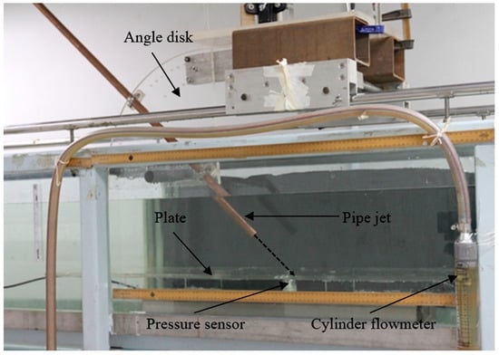
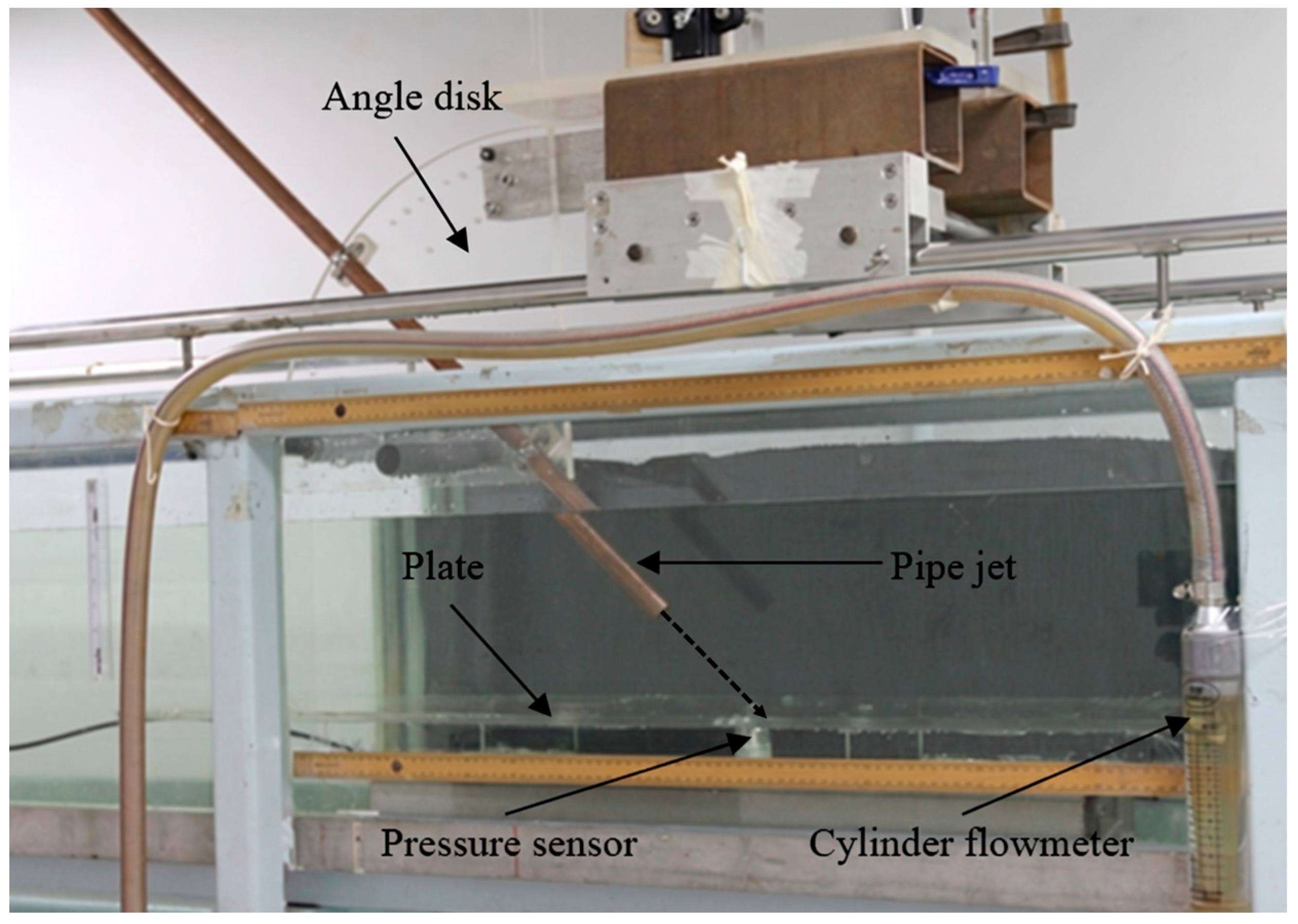
To visualize the flow structure of submerged impinging jets, an experimental circuit was assembled as shown in Figure 1. The setup included a water tank, an angle disk, an adjustable-angle copper pipe, an impingement plate, gate valves, pressure sensors, flow meters, a magnetic pump, etc. The circulating water used in the experiment is clear water, the density ρ = 1000 kg/m³, the water temperature T₀ = 20 °C, and the tank’s surrounding and bottom wall are made of single-layer transparent tempered glass. The jet fluid flows into the water tank through a circular copper pipe with dimensions of L = 1200 mm and d = 20 mm. The copper pipe length ensures jet flow reaches full development before entering the water tank. Using the diameter to non-dimensionalize the length, which is expressed as L = 60d, the copper pipe is installed on the angle disk in the middle cross-section of the tank, which is far away from the vertical wall surface of the water tank. The jet impingement angle θ can be adjusted with the angle disk, ranging from 0° to 90°. The jet flow velocity U_j is controlled by pumps and valves, and the accuracy of the flow rate is ± 0.5%. In this study, the nozzle exit velocity U_j is 1.17 m/s, which corresponds to a Reynolds number (Re) of 23,400 (Re = ρU_jd/μ, where, in this case, μ is the viscosity coefficient of fluid, μ = 1.0028 × 10⁻³ Pa·s; d represents the nozzle diameter). The vertical distance between the exit of the copper pipe and the impingement plate is the impact height H, which is set to a constant value H/d = 3 in this study.

Figure 1. Experimental setup of submerged impinging jet.

The experiment employed a dual-frame/double-exposure PIV system to measure the flow velocity in the test plane. Two Yttrium Aluminum Garnet (YAG) lasers of type NL100-50 (Ekspla, Vilnius, Lithuania) were positioned at the bottom of the water reservoir; the laser sources delivered pulsed sheet illumination to the test plane. The laser operated with a pulse energy of 135 mJ per pulse, a wavelength of 532 nm, and a pulse width of 5 ns. Hollow glass spheres served as seeding particles for flow visualization, which have the following main parameters: an average diameter of 13 μm, an average relative density of 1.1, with good traceability and scattering efficiency. The flow field was captured using a CCD camera with a resolution of 1600 × 1200 pixels. Through target calibration, the physical size of the field of view was determined to be 160 mm × 120 mm, yielding a spatial resolution of 10 pixels/mm. The image pairs were acquired at a sampling frequency of 15 Hz. While this relatively low acquisition rate is insufficient to fully resolve the high-frequency transient time scales of the turbulent flow, it is thoroughly adequate for computing statistically converged time-averaged flow characteristics. In this study, an ensemble of 1000 instantaneous image pairs was accumulated for each test case to extract reliable mean velocity fields and Reynolds stresses. Referring to this literature, the time interval Δt between continuous laser pulses is between 400 μs and 700 μs [21]. Using the cross-correlation algorithm based on fast Fourier transform (FFT), the standard Gaussian sub-pixel filter (LaVision GmbH, Göttingen, Germany) was implemented as an iterative multi-grid method to calculate the particle displacement vector map. Combined with the time interval, the velocity vector distribution in the plane was finally obtained. To ensure the reproducibility and clarity of the experimental methodology, the spatial calibration and temporal resolution parameters are reported following the highly structured framework suggested by Brazhenko [22]. The pressure was measured by a pressure sensor installed on the impingement plate. The sensor model is Keller PR41-X (Keller PR41-X, KELLER Pressure, Winterthur, Switzerland), with an accuracy of ±0.3% and a measurement range of 0–30 mbar.

3. Numerical Simulation Method

In the study, Wray-Agarwal, RNG k-ε, SST k-ω turbulence models, and the LES method were used to simulate the flow field characteristics of submerged impinging jets at multiple impact angles.

3.1. Mesh Generation, Boundary Conditions Setting, and Free Surface Treatment

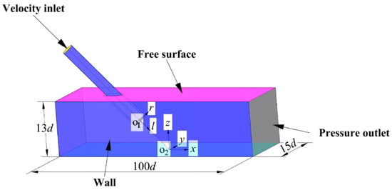
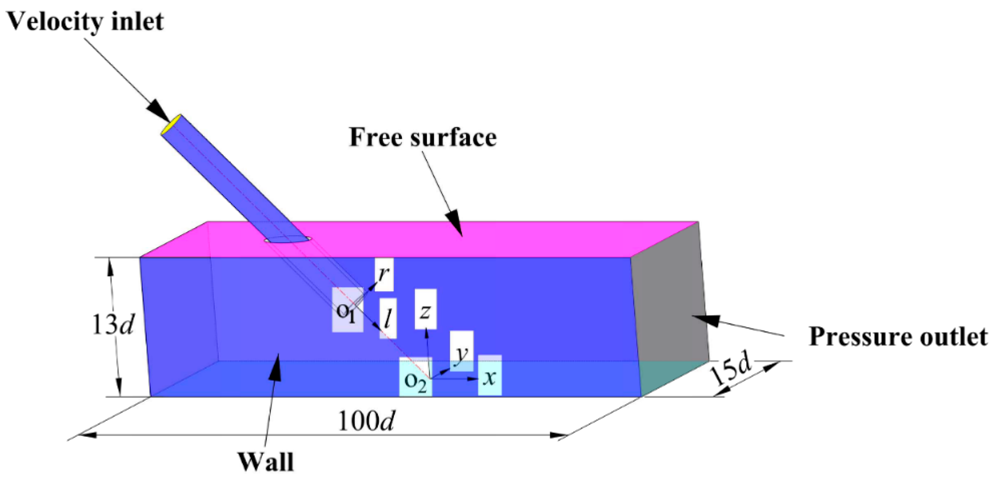
Figure 2 is the calculation model of the submerged impinging jet impinging on the wall. The nozzle’s internal diameter is used to non-dimensionalize the size of the water tank, which can be described as 100d × 15d × 13d. To facilitate the description of the flow field structure in different flow regions, two coordinate systems, rO₁l and xO₂yz, are established. The coordinate origin O₁ is located at the centerline of the pipe exit, with r and l representing the radial and axial directions of the pipe, respectively. The intersection between the nozzle axis and the impinging wall serves as the coordinate origin, O₂. The x, y, and z denote the longitudinal, lateral, and vertical dimensions of the reservoir, respectively.

Figure 2. Computational domain and boundary definition of submerged impinging jet.

In this model, the flow medium is an incompressible fluid, and the boundary conditions are set as follows: a velocity inlet of 1.17 m/s is applied at the copper pipe entrance. The walls on both sides of the tank in the width direction are defined as pressure outlets, set to 0 MPa. The remaining two side walls and the bottom of the water tank are set as smooth, non-slip boundaries. Since the primary objective of this study is the comparative assessment of different turbulence models in predicting the internal flow mechanisms, the symmetry boundary assumption is strategically employed for the free liquid surface at the top to avoid airflow interference with the jet flow region. Physically, this assumption is strictly valid for subcritical flows where surface perturbations are minimal. For the present configuration, the Froude number is calculated to be Fr = 0.8357, ensuring that free-surface deformation is negligible and air entrainment is entirely absent, thereby physically justifying the rigid-lid approach. Furthermore, this approach isolates the turbulence modeling evaluation from multiphase complexities, ensuring a methodologically sound and fair comparison of the models’ intrinsic predictive performances.

For the RANS approach, the iterative solution process was governed by strict convergence criteria. The simulations were deemed converged only when the scaled residuals for all governing equations, including the continuity, momentum, and relevant turbulence transport equations, fell completely below 10⁻⁵. The total number of iterations is 25,000. The pressure–velocity coupling was resolved using the SIMPLEC algorithm. Spatial discretization of the convective terms was handled via the Second-Order Upwind scheme, and the enhanced wall treatment was applied to accurately resolve the viscous sublayer for the RANS models. When using large eddy simulation, the bounded central differencing scheme was strictly employed to avoid excessive artificial dissipation. The transient formulation utilized the bounded second-order implicit scheme. Since the initial conditions have a great influence on unsteady calculations, the LES method has high requirements for convergence conditions. Therefore, in order to enhance simulation accuracy and convergence rate, the simulation results of the flow field from the RNG k-ε turbulence model were used as the initial values for LES. The WALE subgrid-scale model in LES naturally resolved the near-wall gradients without explicit wall functions. The transient control equations are discretized using the finite volume method, with a second-order implicit scheme for solving the time integration, and the convection term is implemented using a central difference format.

3.2. Grid Independence Analysis

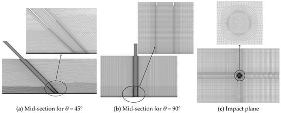
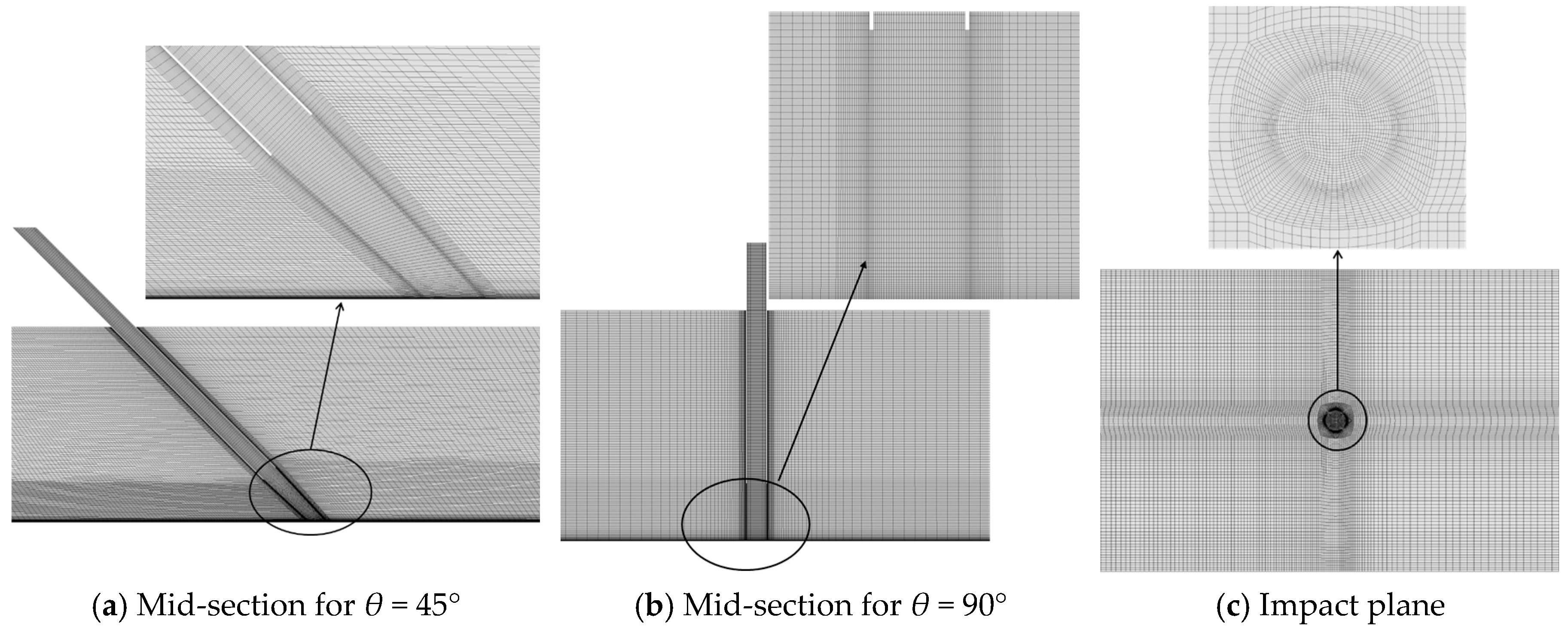
Considering that the jet outlet is circular and the main computational domain is a rectangular prism, a region-based meshing strategy is adopted. Additionally, according to the flow features of the submerged impinging jet field, local refinement is applied to regions with high velocity gradients, including the jet core region, impact region, and boundary layers. The specific mesh division is shown in Figure 3. The grid sizes listed in Table 1 represent the global element seed sizes (maximum element sizes) applied to the computational domain, defined in millimeters (mm). Meanwhile, the grid growth rate is carefully controlled to ensure that most grid cells are concentrated in the jet core region and near the impact region, while the uniform flow area uses sparse grids. To eliminate the influence of grid factors on numerical calculation results and ensure computational accuracy, four grid schemes under the working condition of the impinging angle θ = 45° were designed for comparative analysis. The first wall-layer grid height is uniformly set to 0.1 mm, with the highest mesh density on the impinging wall. The detailed grid setting is as follows.

Figure 3. Computational domain grid of submerged impinging jet [22].

Table 1. Grid division scheme.

Scheme	Grid Size	Grid Growth Rate	Number of Water Tank Nodes (Length × Width × Height)	Grid Number of Pipe	Grid Number of Tank	Total Grid Number
1	1.5	1.05	368 × 140 × 184	658,107	11,857,340	12,515,447
2	2.0	1.1	320 × 120 × 160	393,479	6,362,713	6,756,192
3	2.5	1.5	256 × 96 × 130	198,113	3,559,767	3,757,880
4	3.0	2.0	203 × 77 × 100	107,528	1,607,940	1,715,468

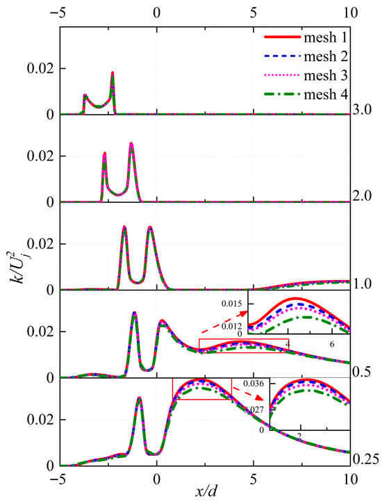
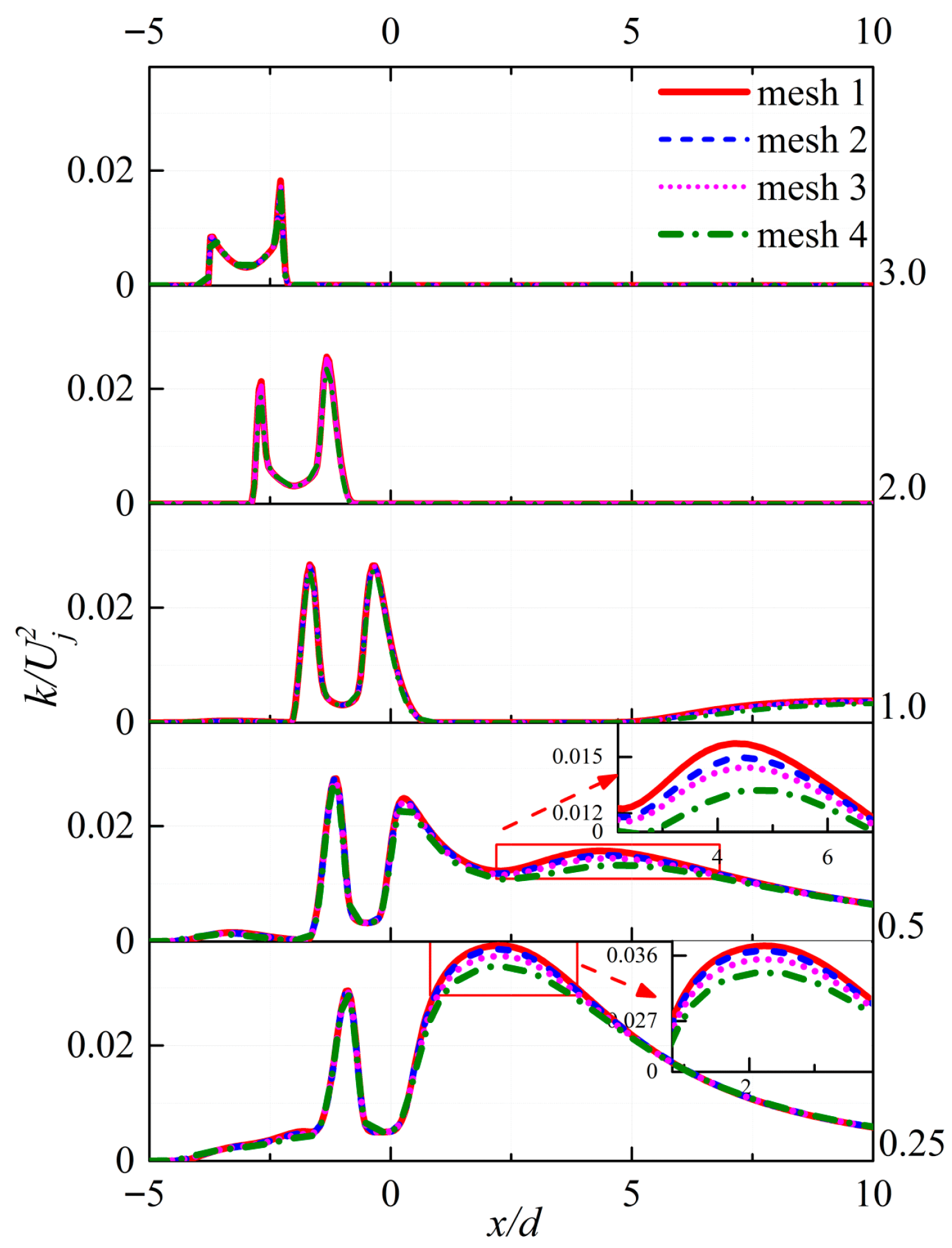
In order to improve calculation efficiency, the RNG turbulence model was used to carry out trial simulations on the geometric models of the above four grids. The influence analysis of the grid number on velocity under different grid schemes can be found in this paper [23]. The dimensionless turbulent kinetic energy, k/$U_j^2$, which is highly sensitive to grid resolution in the shear layer and near-wall regions, was selected as another monitor variable. Figure 3 presents the distribution of turbulent kinetic energy k/$U_j^2$ along the radial direction at different heights (z/d). In the vicinity of the nozzle exit, the distribution of k/$U_j^2$ at the same height is basically the same, with the peak value located in the shear layer of the jet, decreasing radially toward the jet axis. In the initial shear layer, the k/$U_j^2$ near the nozzle exit, calculated by the fourth grid scheme, is slightly lower. With the development of the jet, more external fluid is entrained into the jet core across the shear layer, resulting in intensified flow mixing. The shear layer becomes unstable from the periphery toward the jet centerline. Meanwhile, the turbulent kinetic energy, which is relatively low in the upstream, is transferred to the downstream and further amplified. Consequently, it affects the prediction results of the impingement region and the wall-jet region. As shown in Figure 4, at the near-wall location of z/d = 0.25, refining the grid scheme from scheme 4 to scheme 3 results in a noticeable reduction, with a maximum of approximately 5.53%. As the grid is further refined, the maximum relative percentage difference in k/$U_j^2$ between scheme 2 and scheme 1 is only 1.79%; however, the number of grids is also doubled. Furthermore, to systematically quantify the discretization error, a formal grid sensitivity study was conducted following the Grid Convergence Index (GCI) procedure recommended by Semlitsch [24]. Based on the three representative grids (scheme 2, scheme 3, and scheme 4), the apparent order of the method, k/$U_j^2$, was evaluated. The values of GCI₄₃ and GCI₃₂ are 3.7 and 1.38, respectively. It means that the numerical solutions are within the asymptotic range of convergence, and mesh 2 is sufficiently resolved for the present analysis. Therefore, to optimize computational efficiency without compromising physical fidelity, mesh 2 was adopted for all subsequent numerical investigations.

Figure 4. Distribution of turbulent kinetic energy along the radial direction at different heights (z/d).

3.3. Time Step Independence Verification

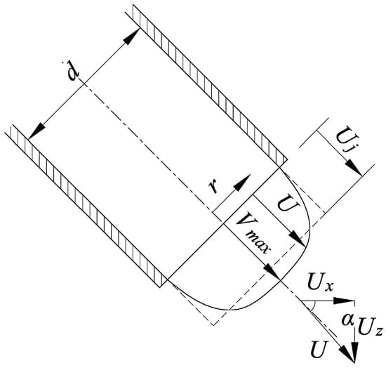
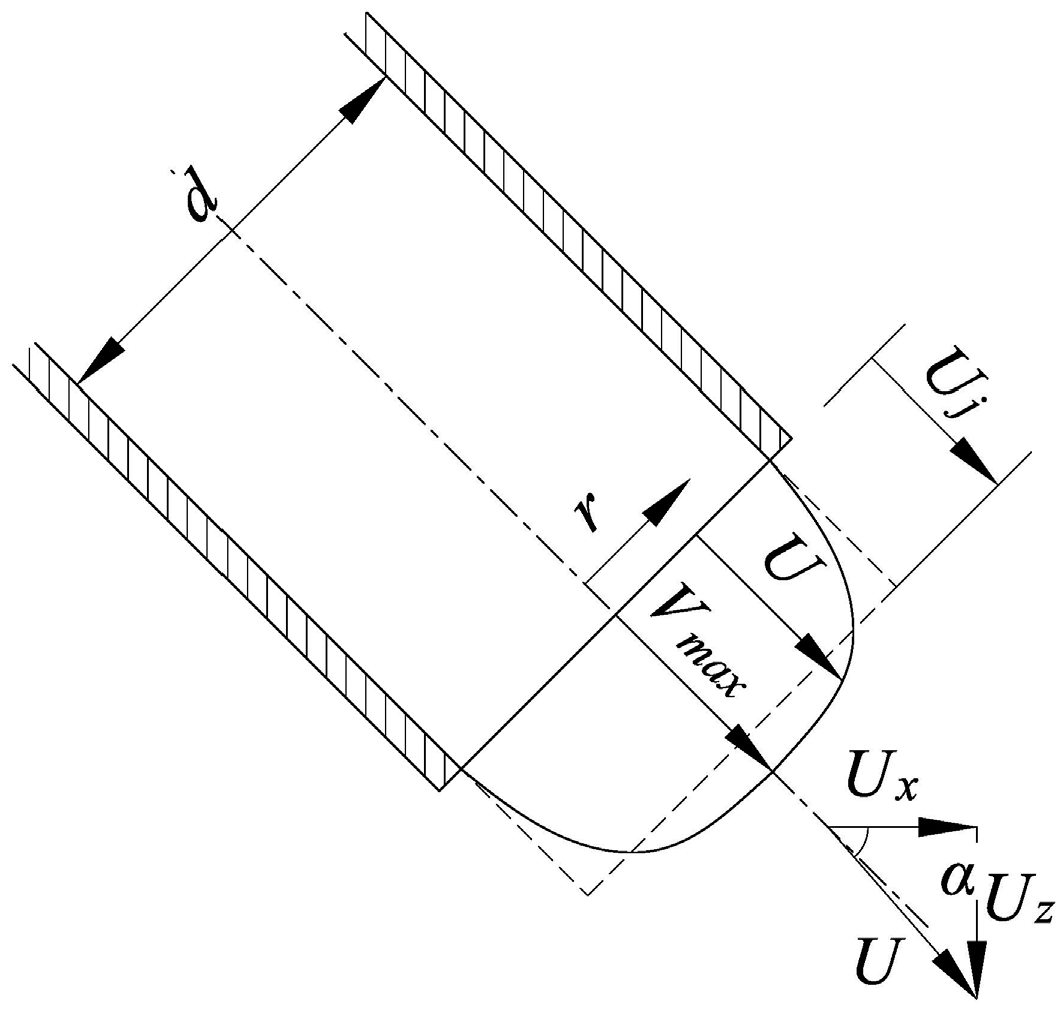
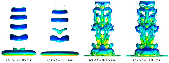
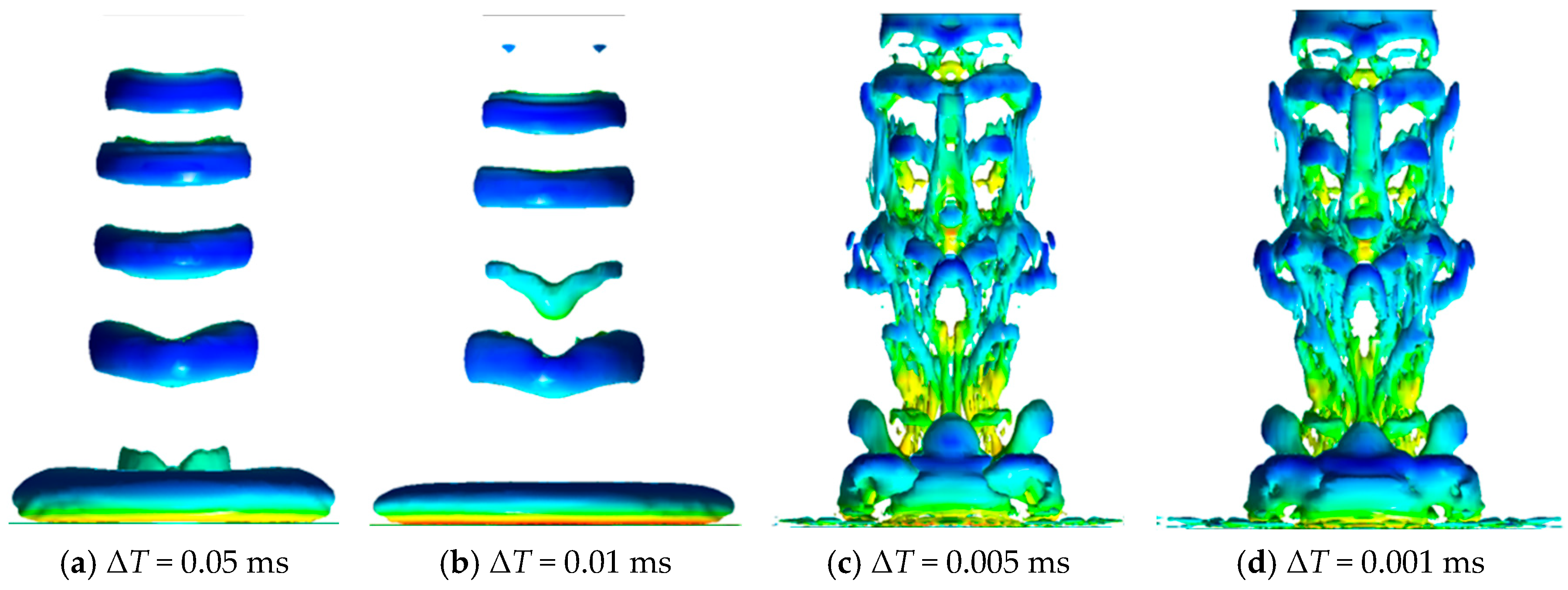
In the LES method, the time step needs to meet ΔT ≈ Δx/V_max, where Δx is the minimum grid size of 0.1 mm, and V_max is the maximum velocity in the nozzle exit, which is equal to 1.2U_j and shown in Figure 5. In order to eliminate the influence of time step ΔT on the accuracy of numerical simulation, four different time steps are selected in this paper: 0.001 ms, 0.005 ms, 0.01 ms, and 0.05 ms [25]. The remaining simulation parameters are kept identical. Figure 6 shows the distribution comparison of vorticity isosurfaces under four kinds of time step settings at the same time. The figure illustrates that the time step significantly impacts the vorticity isosurface of the jet. The characteristics of different-scale coherent structures in the jet flow field can be well represented under ΔT = 0.001 ms and ΔT = 0.005 ms, and the two show little difference in the scale of vortex structure. However, when using ΔT = 0.01 ms and ΔT = 0.05 ms, some small-scale vortex structures are eliminated. Therefore, considering the influence of time step on computing resources requirements and computational accuracy, the time step ΔT = 0.005 ms was selected for the unsteady numerical simulation in this paper. Under this configuration, the Courant Friedrichs Lewy (CFL) number (CFL = U_j*ΔT/Δx = 0.88) satisfies the requirement of CFL < 1 for large eddy numerical simulation calculations.

Figure 5. Diagram of velocity flow angle and all kinds of velocity.

Figure 6. Isosurface of Q-criterion (Q = 0.2) at different time steps.

4. Comparative Study of Various Numerical Approaches in Submerged Impinging Jets

4.1. Simulation Results for the Free Jet Region Based on Various Turbulence Models

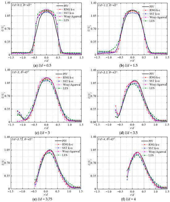
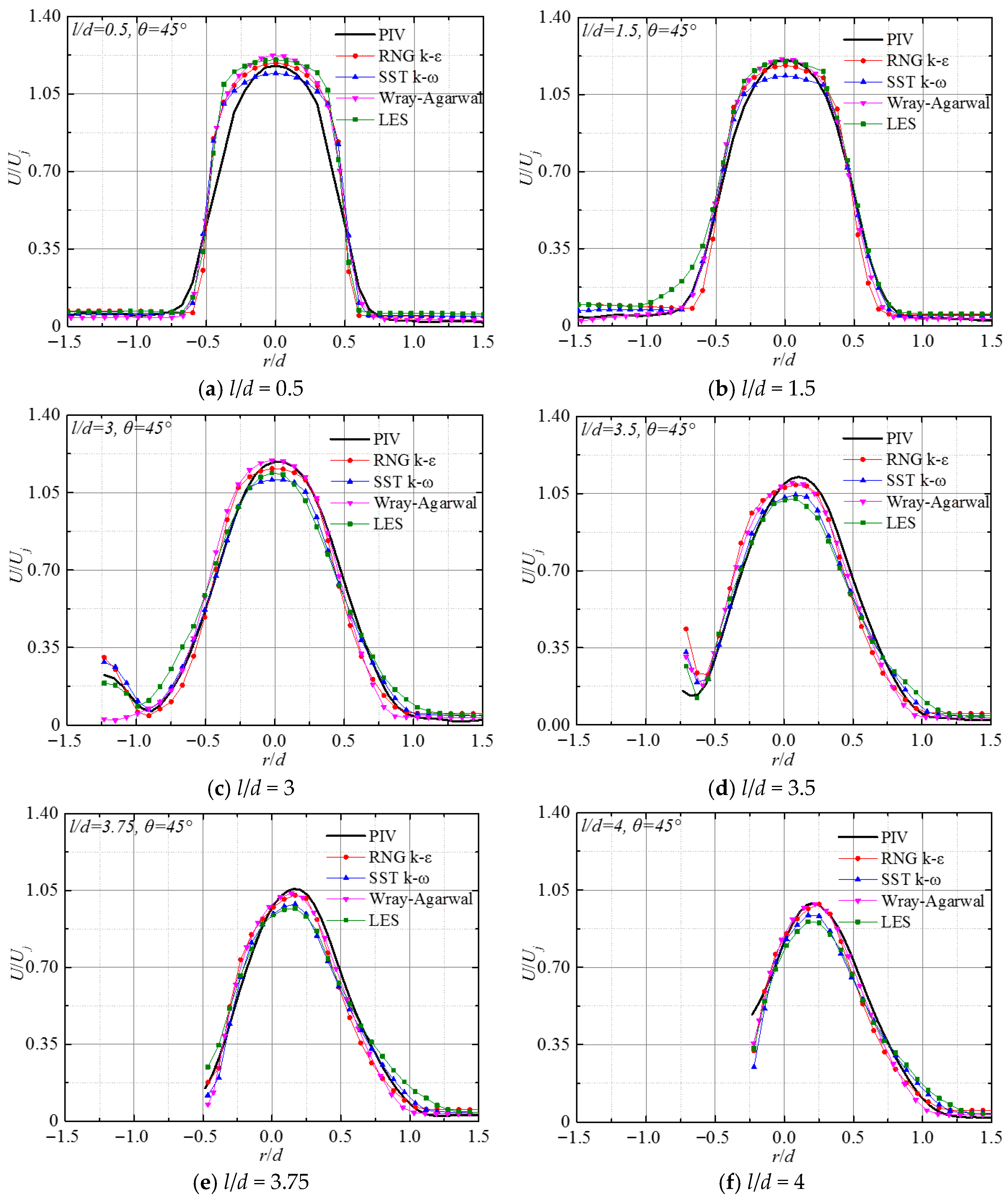
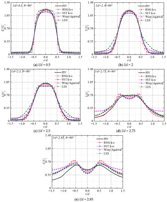
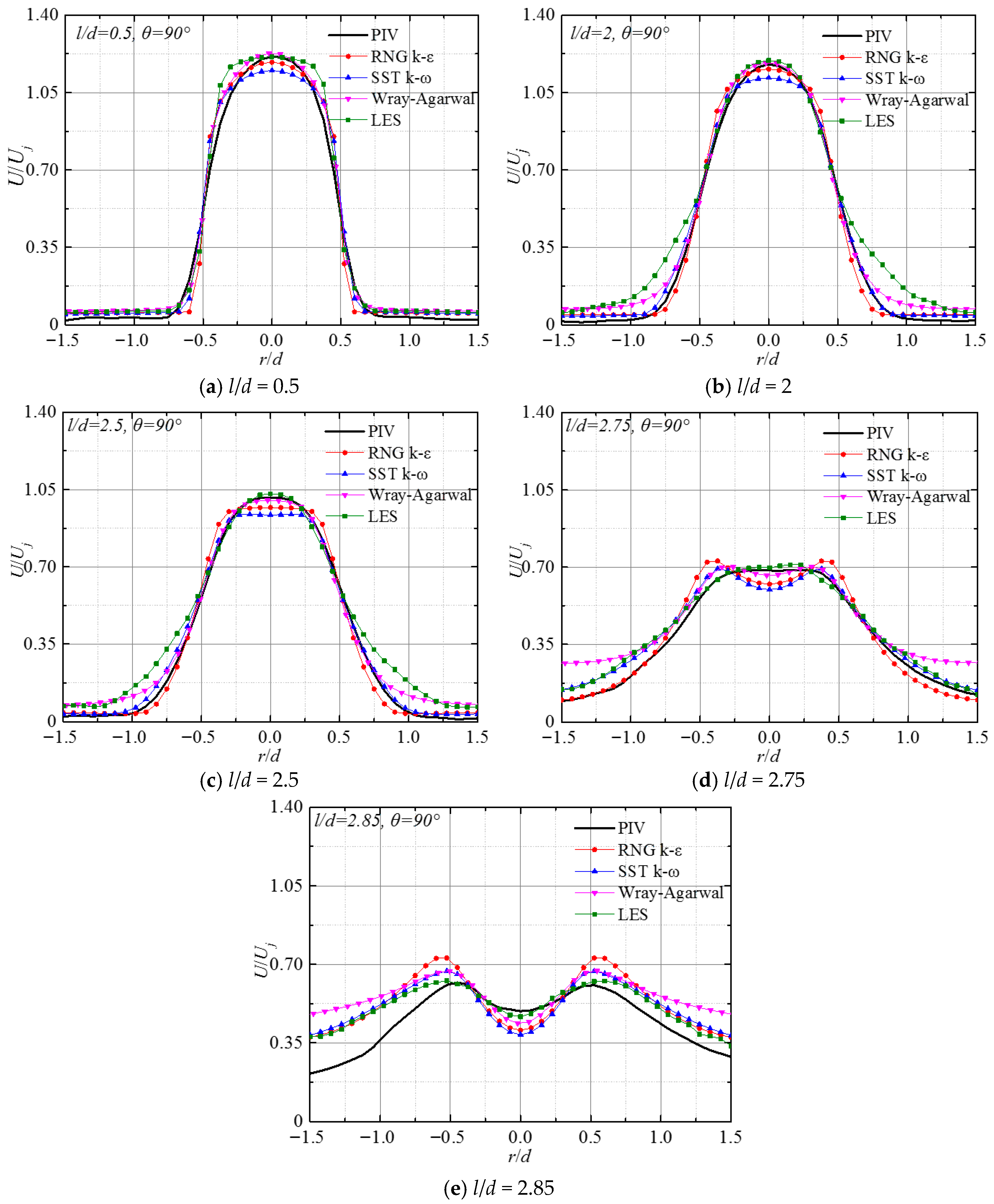
Figure 7 and Figure 8 display the dimensionless mainstream velocity along the radial direction for a submerged impinging jet with impact angles of 45° and 90° under different numerical simulation methods. The corresponding experimental results are also included in the figures. When θ = 45°, all the simulated radial velocity distributions at different axial positions of the jet result in matches to the experimental values well. At the jet exit, U/U_j exhibits nearly axisymmetric distribution along the radial direction, with the maximum velocity occurring at the axis line. Along the development direction of the jet, this symmetry is weakened, and the location of peak velocity gradually migrates away from the axis. Figure 7 reveals that, in the potential core slightly beyond the nozzle outlet (l/d = 0.5), the discrepancy between the simulated results and the experimental measurement reaches its maximum. The numerical values obtained using the RNG k-ε, W-A turbulence models, and LES method are higher than those of the experimental measurements, while the numerical simulation values from the SST k-ω turbulence model are lower than those measured experimentally. When the flow develops to l/d = 1.5, as depicted in Figure 7b, the predictions from RNG k-ε, W-A model, and LES are very close to the experimental values, and the numerical results of the SST k-ω turbulence model still differ significantly from the experimental values. As the flow develops, at l/d = 3, the calculation results of the LES method are gradually lower than the experimental results. At this time, the main part of the jet fluid (r/d = −1.23) reaches the impinging wall, and the peak velocity location on the cross-section progressively shifts from the jet centerline. In a free jet zone, the flow exhibits a strongly anisotropic shear layer separating the jet from the surrounding fluid with rapid strain rates and intense entrainment. The RNG k-ε model’s advantage is due to its dissipation equation (ε) and an additional strain-rate-dependent term (R_ε). Especially in the rapidly strained shear layer, the term profoundly enhances the rate of dissipation, thus physically suppressing the unphysical generation of turbulent kinetic energy and correctly predicting the narrow spreading rate of the jet core. Generally, simulation results of the RNG k-ε turbulence model and the W-A turbulence model show better agreement with experimental data than those of the SST k-ω model, while LES does not achieve particularly high consistency with the experimental results. For θ = 90°, the peak point of the dimensionless velocity U/U_j obtained by numerical simulation is identical to the experimental results. U/U_j exhibits good symmetry along the radial direction at different axial positions, and a steady decline in the maximum velocity is observed along the jet axis. Figure 8a shows that near the nozzle exit, there are some deviations between the four numerical calculations and the experimental results, among which the deviation of SST k-ω is the largest. As the jet develops, the predicted results of the LES method gradually approach the experimental values, and when l/d > 2, they are almost consistent in the range of 0.5 < r/d < 0.5. In the free-jet core region of the submerged impinging jet at θ = 90°, the results obtained by the LES method are most consistent with the experimental data.

Figure 7. The radial distribution of jet velocity U/U_j at different axial positions for θ = 45°.

Figure 8. Radial distribution of velocity U/U_j at different axial positions for θ = 90°.

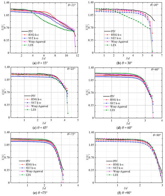
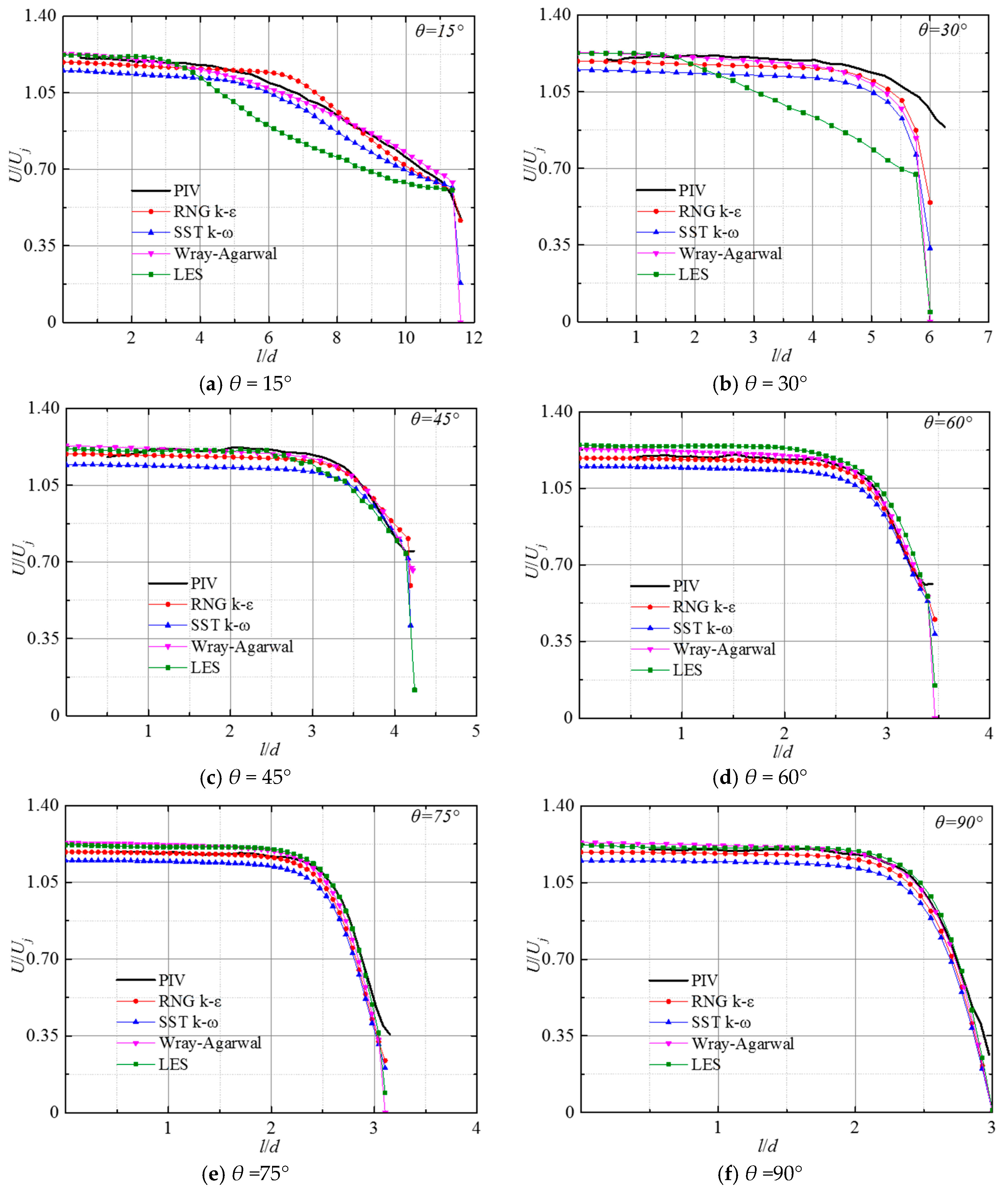
Figure 9 shows the variation in the normalized velocity U/U_j along the jet centerline at Re = 23,400 under several impingement angles (θ = 15°, 30°, 45°, 60°, 75°, and 90°), respectively. It shows that, for various impinging angles, the dimensionless velocity remains consistent within the potential core region; the centerline velocity remains uniform and identical to the nozzle discharge velocity for a specific downstream extent. This area is generally defined as the core area of the jet. Then, the dimensionless velocity U/U_j starts to decay, and its decay rate accelerates with the increase in the impact angle. Under different impinging angles, the length and attenuation trend of the jet core area obtained by RNG k-ε, W-A, and SST k-ω are in good agreement with the experimental measurements. At θ = 15°, the RNG k-ε overpredicts the attenuation of the mainstream, while the SST k-ω slightly underpredicts the mainstream attenuation. When θ ≤ 30°, the predicted value of the W-A model is most consistent with the experimental results, while the attenuation position predicted by the LES method is earlier than the experimental results. This may be due to the fact that the WA is a one-equation model with transporting the ratio of turbulent kinetic energy to R = k/ε, featuring a cross-diffusion term. This allows the model to effectively capture the anisotropic momentum transfer and the highly non-equilibrium turbulence dynamics in the free-jet shear layer, circumventing the excessive diffusion typical of standard Boussinesq-based two-equation models. As the impinging angle increases, the deviation of the four numerical calculations from the experimental results gradually decreases, and when θ increases to 90°, the LES method can accurately predict the axial position where velocity attenuation initiates.

Figure 9. Distribution of velocity U/U_j along the jet axis at different impinging angles.

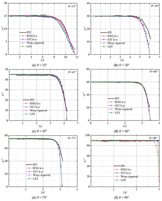
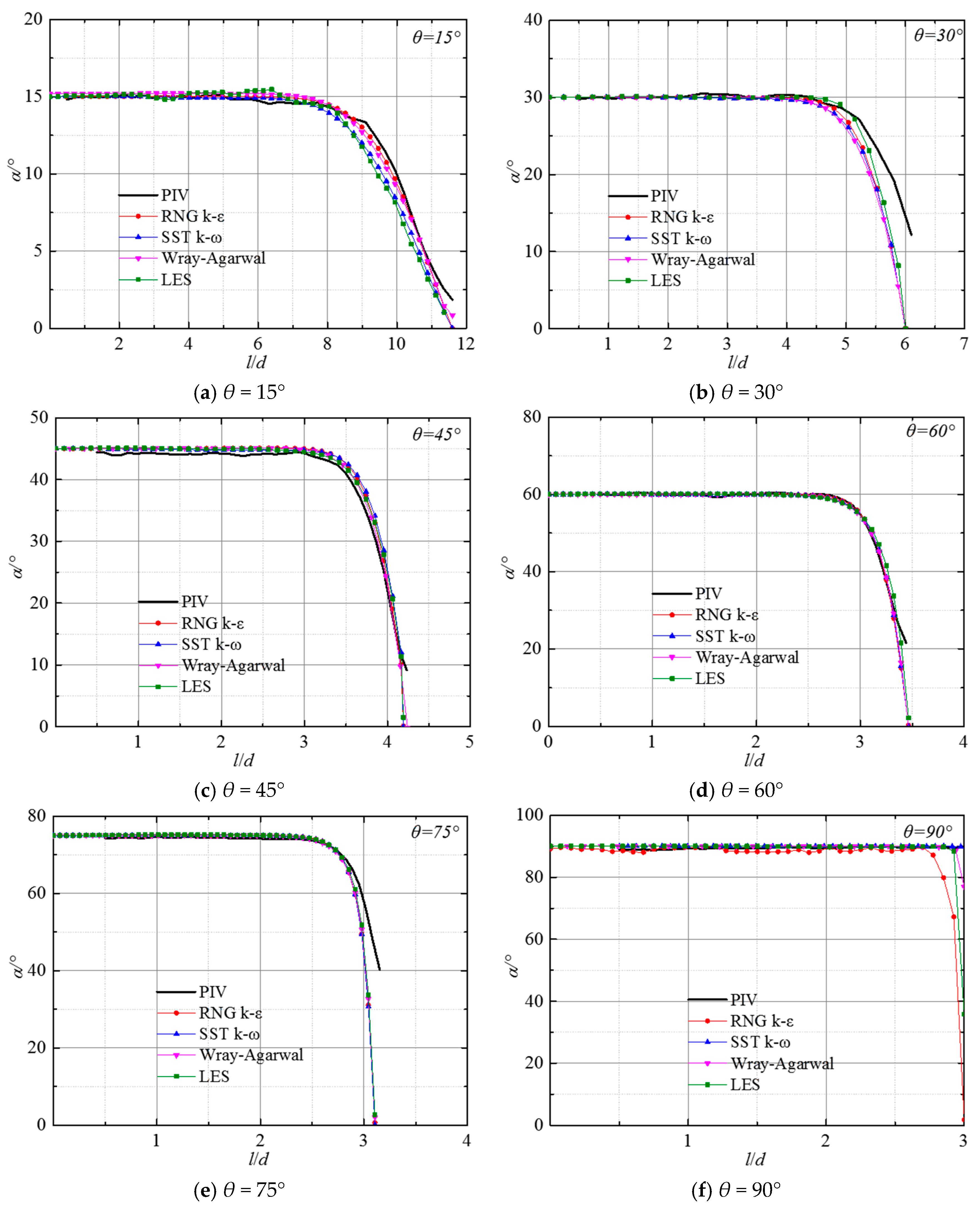
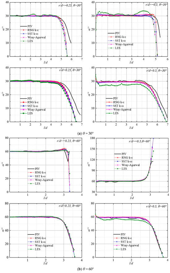
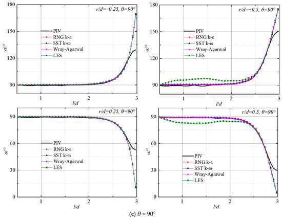
Figure 10 illustrates a comparison between numerical simulations and experimental measurements of the variation in α (flow angle, the definition is shown in Figure 4) on the jet axis for Re = 23,400 under various impingement angles. It can be observed that the distribution trend of the liquid flow angle α along the l-axis obtained by the different numerical simulation methods is basically consistent with the experiments, and the deviation occurs only in the near-wall region. As the increasement of the impact angle, the deviations are further minimized. The larger the impinging angle is, the closer the prediction of α on the jet axis by RNG k-ε and LES is to the experimental value.

Figure 10. Distribution of flow angle α along the jet axis at different impinging angles.

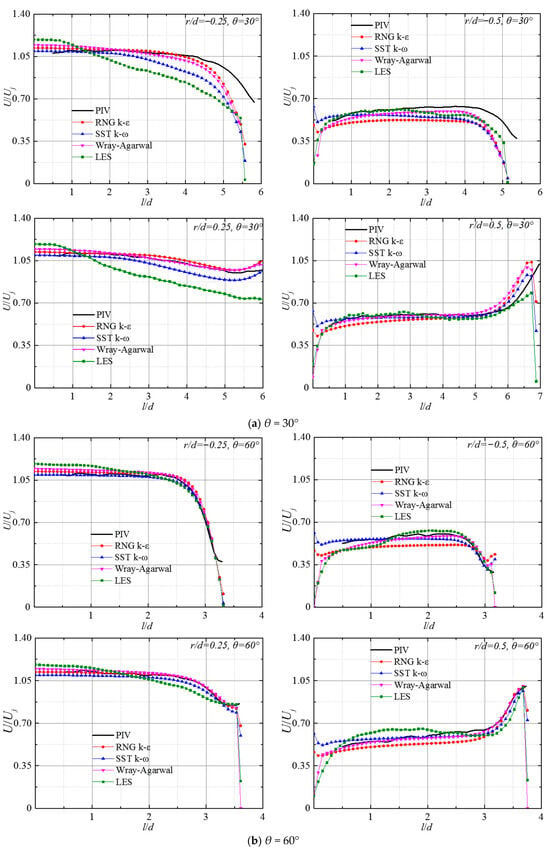
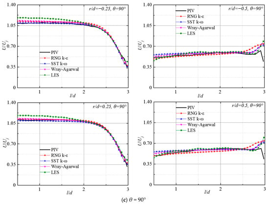
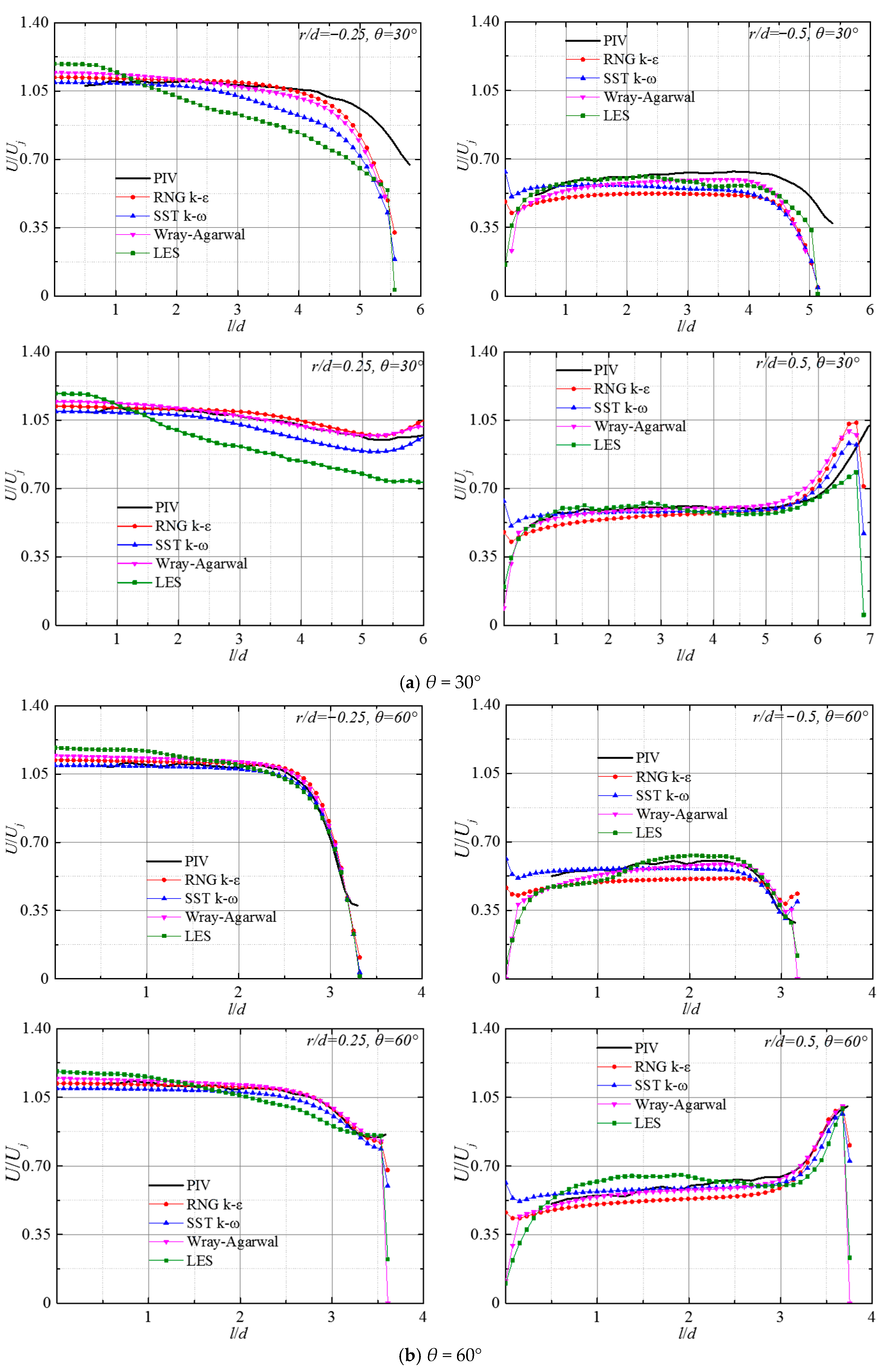
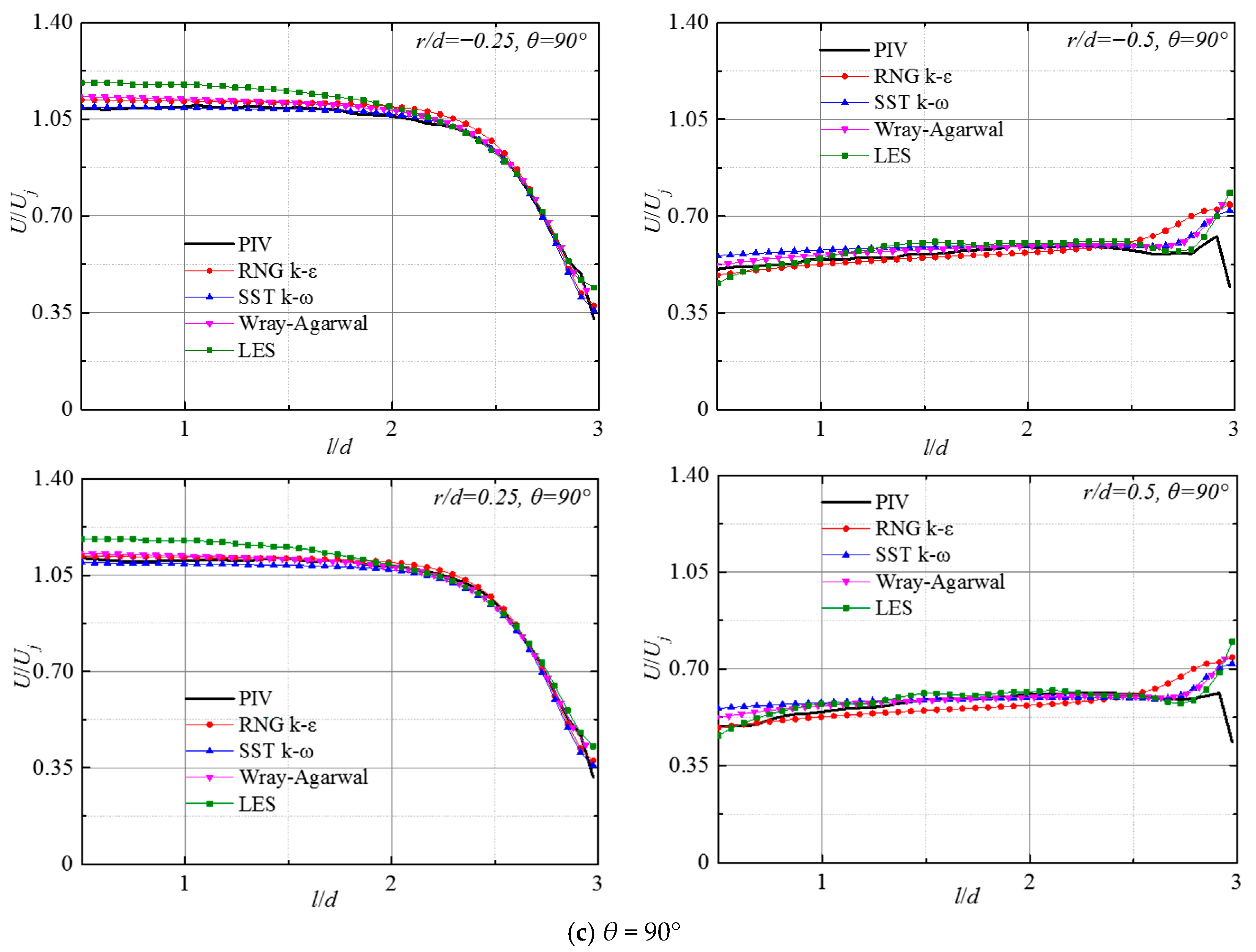
Figure 11 presents the variation in the normalized velocity U/U_j along the axial direction at various radial offsets from the jet centerline on the jet mid-plane for θ = 30°, 60°, and 90° at Re = 23,400. It includes results from various numerical simulations and experimental results. In the free jet zone at r/d = ±0.25, the predicted values of the W-A turbulence model and the RNG k-ε turbulence model always agree well with the experimental results, which accurately reflect the variation characteristics of velocity along the flow direction. In the near-wall impingement zone, numerical predictions begin to deviate. Such deviations are mainly caused by the flow phenomena, including streamline curvature and vortex breakup near the impinging area. When θ ≤ 60°, the deviation of LES prediction results is the largest, while SST k-ω performs slightly better. This deviation gradually decreases with the increment of the impinging angle. When θ = 90°, except that the prediction of the free jet region by the LES method is slightly higher, the other three numerical calculation results exhibit high agreement with experimental results. At r/d = ± 0.5, the predictions of LES and W-A deviate the least from the experimental values. With the increase in the impinging angle, the results of all four numerical simulations gradually approach the experimental values, and at θ = 90°, the results of the LES method almost match the experimental method. This may be due to the fact that the jet generates a highly asymmetric flow field characterized by severe streamline curvature and an unbalanced wall-jet distribution at small impingement angles. The turbulence remains strongly anisotropic in the highly skewed environment. The WALE models in LES inherently assume local isotropy at the sub-grid level. This fundamental assumption breaks down in the intense, asymmetric shear layers of a small-angle oblique impinging jet, leading to significant modeling errors. As the impingement angle approaches 90°, the subgrid-scales become more isotropic, and the LES predictions consequently recover their high fidelity.

Figure 11. Development of normalized velocity U/U_j along axial direction at different radial locations for Re = 23,400.

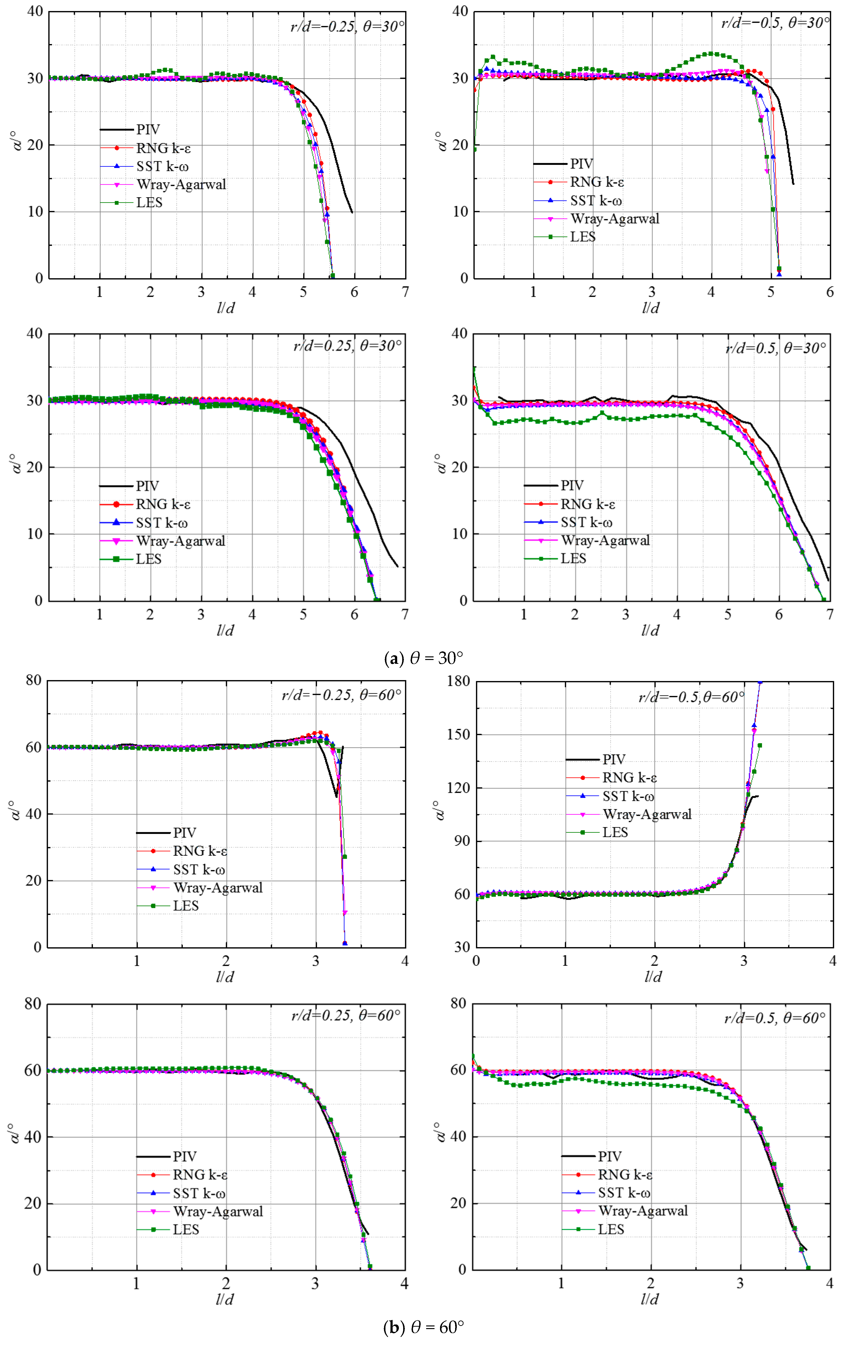
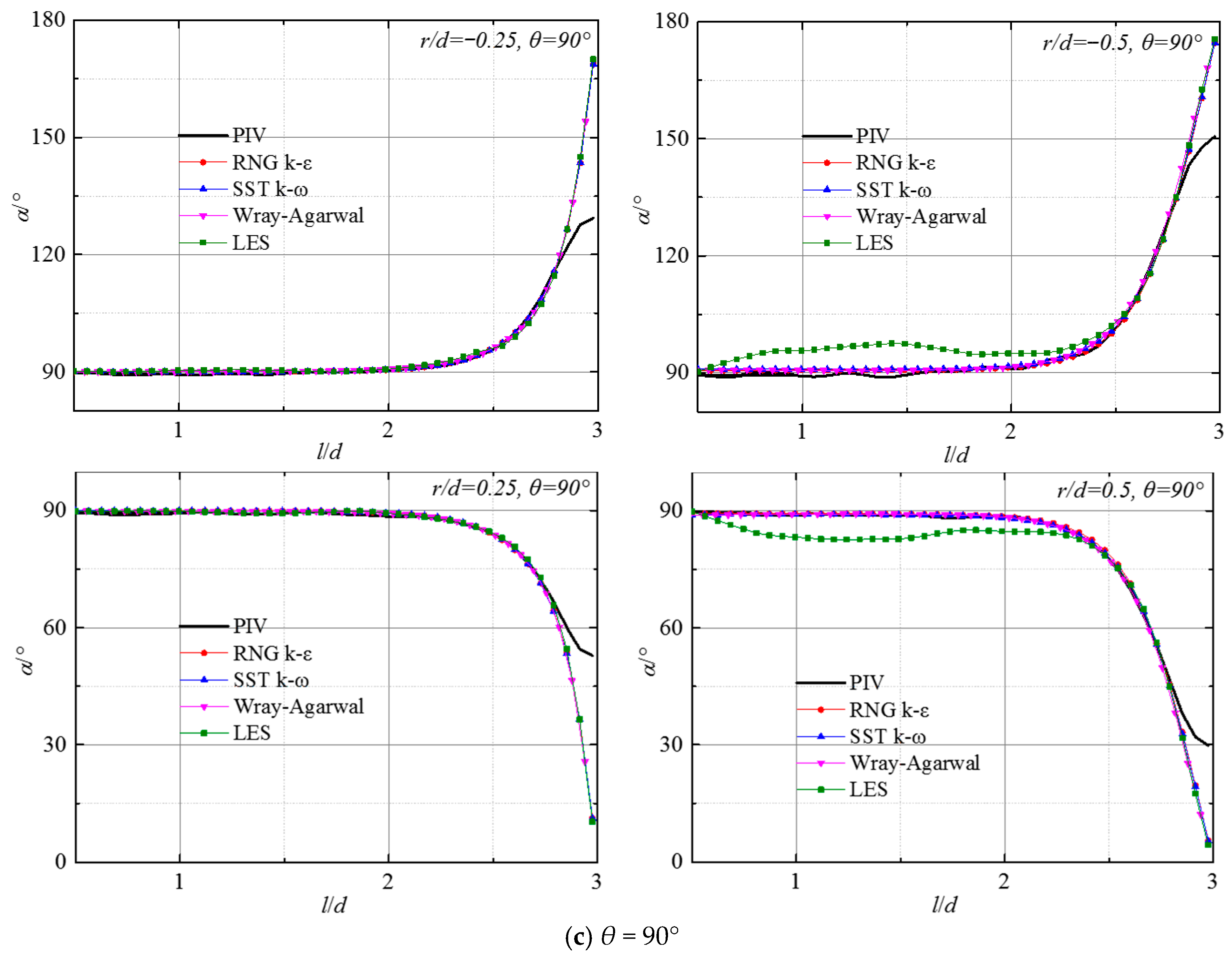
Figure 12 compares the numerical calculations and experimental measurements of the flow angle α in the axial direction at various radial positions under specified jet parameters. It is important to note that the LES approach incurs immense computational costs. Due to these practical computational constraints, the temporal averaging window for the LES statistics was limited. Consequently, minor statistical variations are perceptible in the time-averaged profiles. Rather than applying artificial mathematical smoothing filters, the raw averaged data are presented here to maintain strict methodological transparency. Despite these localized high-frequency fluctuations, monitoring of the flow field confirmed that the macroscopic turbulent structures and the primary mean flow trends had reached a quasi-steady state. The residual statistical noise does not obscure the fundamental physical behaviors, nor does it affect the comparative validity among the evaluated turbulence models. As shown in the figure, at r/d = ±0.25 in the jet core zone, flow angles obtained by the four numerical simulations match the experimental values closely. Notable deviations appear near the wall region, and the magnitude of these deviations gradually decreases as the impinging angle increases. Near the jet boundary layer at r/d = ±0.5, the LES method shows slightly larger deviations from the experimental values than the RNG k-ε, SST k-ω, and W-A turbulence models. This may be attributed to the fact that the WALE model assumes a local equilibrium between turbulence production and dissipation at the sub-grid level, neglecting transport and history effects. In a small-angle impinging jet, the flow encounters severe non-equilibrium dynamics, which are characterized by extreme acceleration on the uphill side and strong adverse pressure gradients inducing flow separation. The inability accounts for these non-equilibrium history effects and leads to deviations in predicting asymmetrical spreading rates.

Figure 12. Development of flow angle α along the axial direction at different radial locations for Re = 23,400.

According to the above analysis, the two-equation RNG k-ε performs the best in numerically simulating the free jet region of submerged jets. The improved performance may result from the inclusion of vorticity or rotational effects in the u_t term of the RNG model, which modifies the turbulent viscosity appropriately and enhances prediction ability [26]. While some discrepancy exists near the wall, the overall tendency and the flow regime changes are largely consistent with the experimental data. In addition, the one-equation W-A turbulence model significantly outperforms the SST k-ω model in terms of predictive accuracy. Furthermore, the four sets of numerical predictions show improving agreement with experimental data as the impingement angle increases.

4.2. Simulation Results for the Jet Wall Region Based on Various Turbulence Models

4.2.1. Speed Distribution Comparison

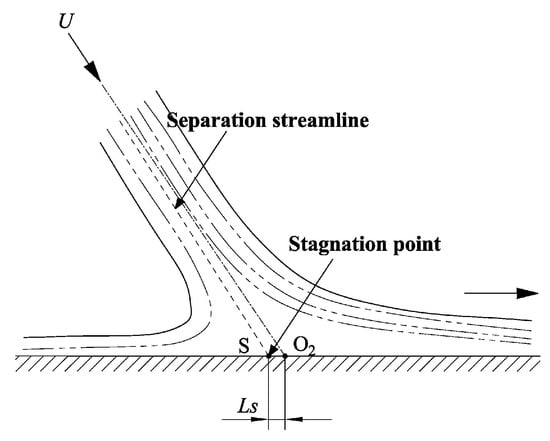
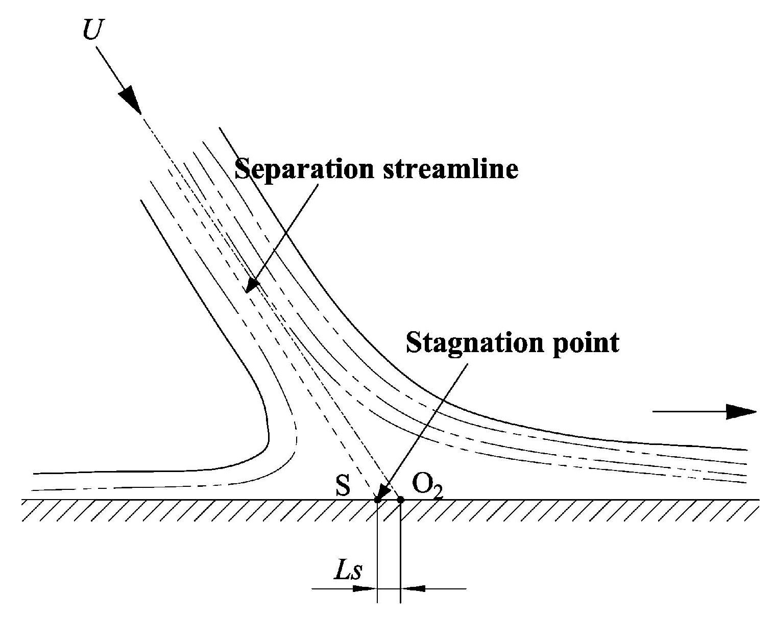
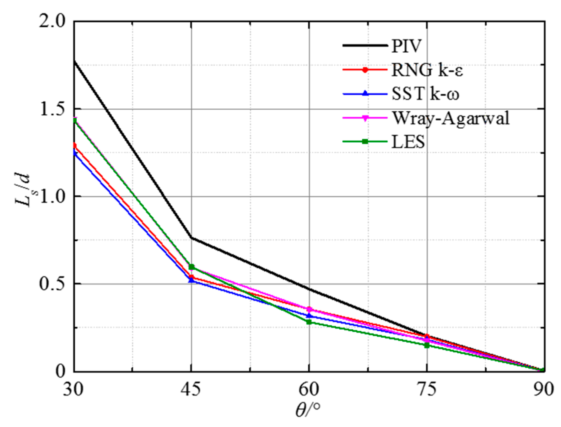
The main body of the jet impinges the wall, then the flow direction changes near the stagnation point, and the main body of the jet diffuses radially around the impinging wall. The stagnation point S is the intersection of the separation streamline and the impinging plane. This point is also the origin of the radial flow, as shown in Figure 13. The geometric center’s distance O₂ from the stagnation point S is marked as L_s.

Figure 13. Diagram of the stagnation point and L_s.

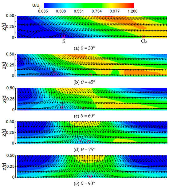
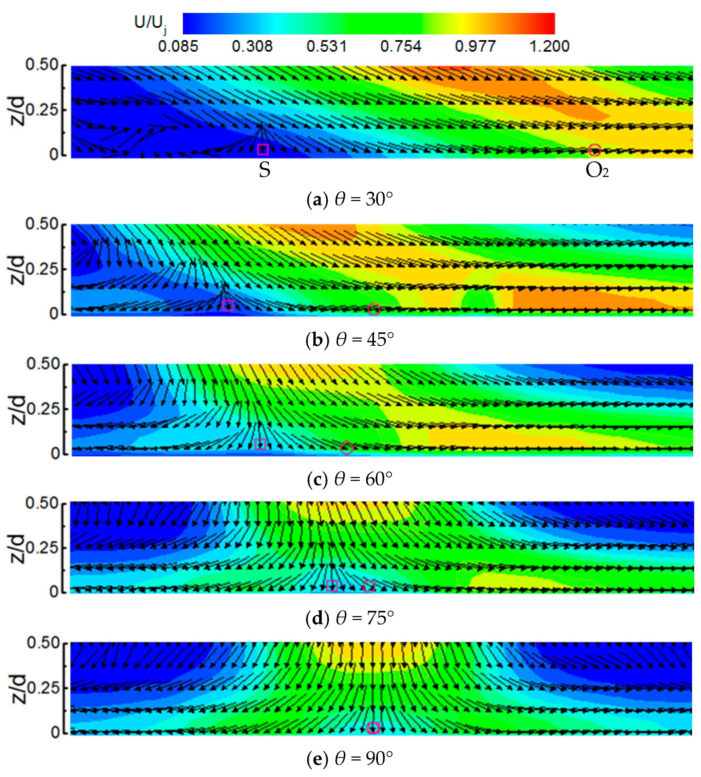
Figure 14 shows the time-averaged velocity vector field and dimensionless velocity distribution of the near-wall region (0 ≤ z/d ≤ 0.5) obtained from PIV at Re = 23,400, H/d = 3 under different impingement angles. The position of the jet stagnation point S (marked by the graphic “□”) and the geometric center O₂ (marked by the graphic “○”) are given in Figure 13. The fluid velocity decreases sharply near the stagnation point, and the flow turns radial on the impinging wall, forming a wall-jet area. The wall-jet region is composed of forward and backward flow in the mid-section of the jet. When the impinging angle is θ = 90°, the stagnation point aligns with the geometrical center, and the flow near the wall shows good axial symmetry. When θ < 90°, the radial flow distribution is gradually inhomogeneous, and with a reduction in the impingement angle, the stagnation point shifts toward the counterflow side (−x), resulting in an increase in L_s. Meanwhile, the flow rate increases along the mainstream direction (+x), accompanied by a prompt increase in the thickness of the shear layer, while the flow rate decreases in the opposite direction of the mainstream, accompanied by a rapid thinning of the shear layer. When the impinging angle decreases to 30°, only a limited volume of the fluid travels against the main flow.

Figure 14. Distribution of velocity vector and cloud map of U/U_j in near-wall region under different impinging angles, ○—geometric center (O₂), □—stagnation point (S) for Re = 23,400, H/d = 3 at different impinging angles.

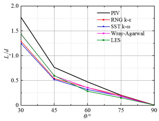
As shown in the above figure, the geometric center O₂’s distance from the stagnation point S changes rapidly with the impinging angle, which makes the distance “L_s” an important flow parameter in the vicinity of the wall. Figure 15 compares the L_s/d values calculated by the four numerical simulation methods with experimental results for various impinging angles. The stagnation point obtained from numerical simulations is generally consistent with experimental measurements. The results from different numerical simulation methods show the same trend as that of the experimental measurements, with L_s/d increasing as the jet impinging angle decreases. The figure also shows that there is a certain deviation between computational and experimental results. For lower impinging angles, the LES provides the least deviation from experimental data. The main reason is that jet deflection on the impingement surface causes vortex fragmentation and attenuation, while the one-equation and two-equation turbulence models are developed based on the assumption of eddy viscosity homogeneity, which inherently limits the ability to accurately predict such flow patterns. However, as the jet impact angle increases, the influence of the upstream wall on the flow is reduced, and this deviation gradually diminishes, approaching the experimental results.

Figure 15. Variation in normalized distance L_s/d with impinging angle.

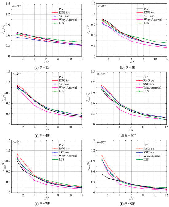
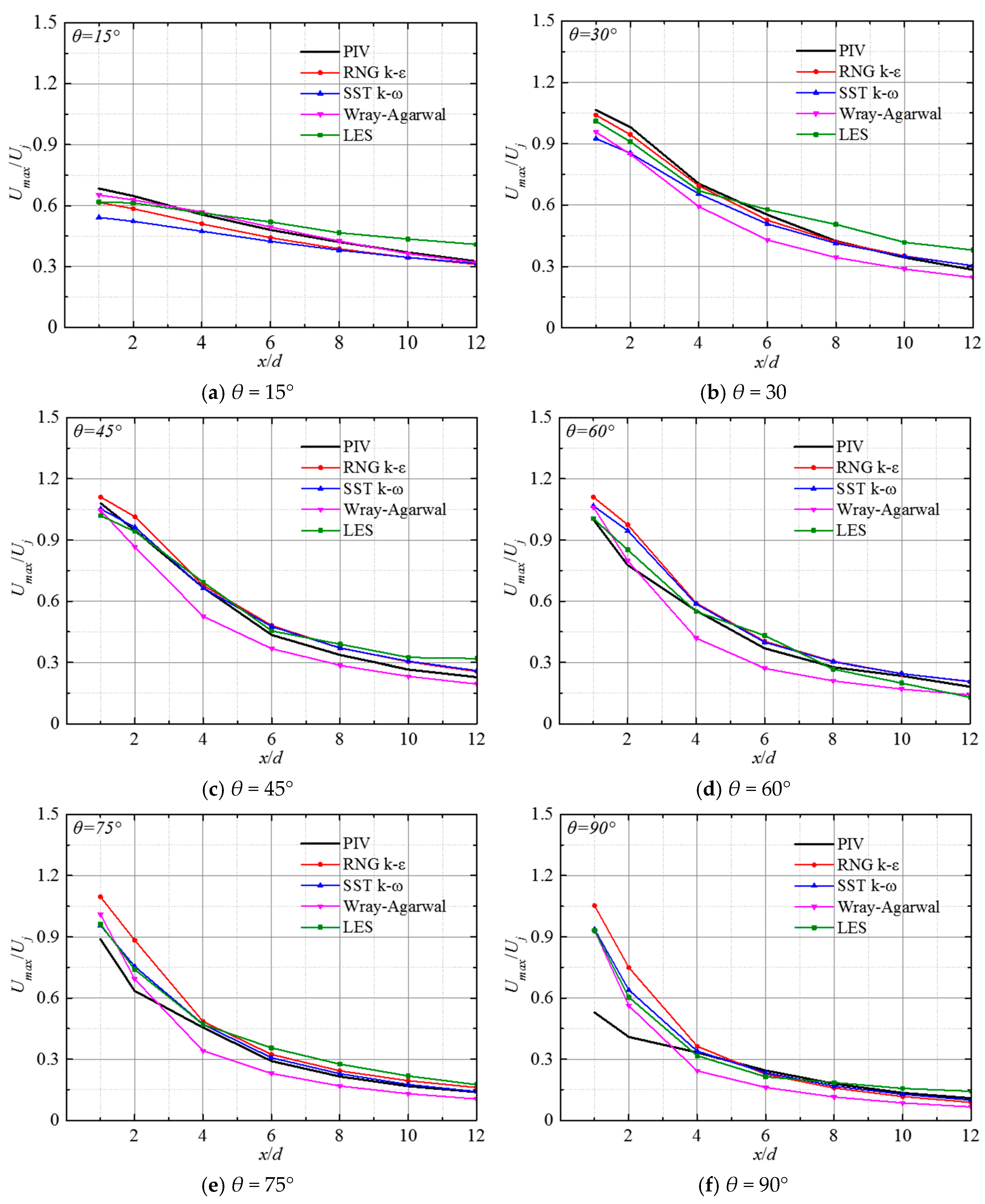
Figure 16 shows the comparison between computational and experimental results for the distribution of the maximum streamwise dimensionless velocity U_max/U_j in the jet mid-section at Re = 23,400, H/d = 3, and θ = 15°, 30°, 45°, 60°, 75°, and 90°, respectively. U_max/U_j decreases gradually along the x-direction. When θ = 15°, the results from the W-A turbulence model are closest to the experimental result. As the impinging angle increases, the deviation between the W-A model predictions and experimental values becomes pronounced, but the consistency of the trend is maintained. As the flow develops downstream, the decay rate of the peak velocity gradually diminishes. The reason for this phenomenon may be that after the jet reaches the impinging wall, the free jet transforms into a wall jet. The larger the impact angle is, the stronger the streamline curvature at the impinging wall is. This finding further demonstrates that the W-A model exhibits limitations in capturing flows with intense rotation and curvature. As the impinging angle increases, the difference between the predicted values of RNG k-ε, SST k-ω, and LES, and the experimental values becomes progressively smaller. When θ > 60°, within the range of x/d < 4, discrepancies between simulation results and experiments gradually increase. When x/d ≥ 4, the results of RNG k-ε, SST k-ω, and LES tend to be consistent with the experimental distribution.

Figure 16. Normalized maximum velocity U_max/U_j of the wall jet along the plane in the forward flow direction for Re = 23,400, H/d = 3, at different impinging angles.

4.2.2. Pressure Distribution Comparison

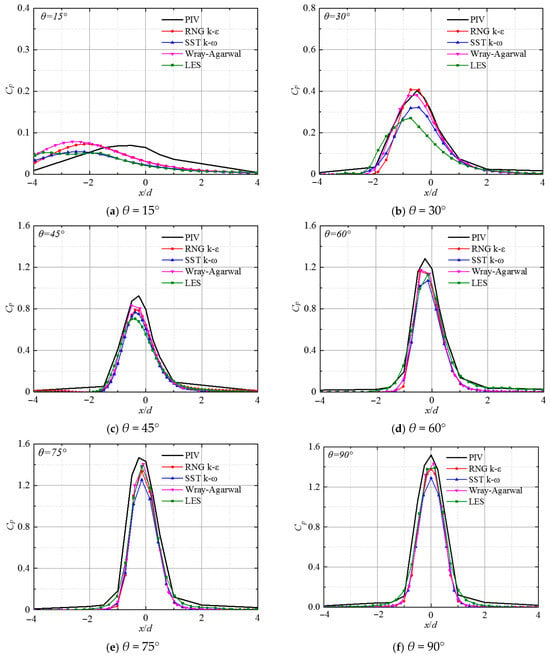
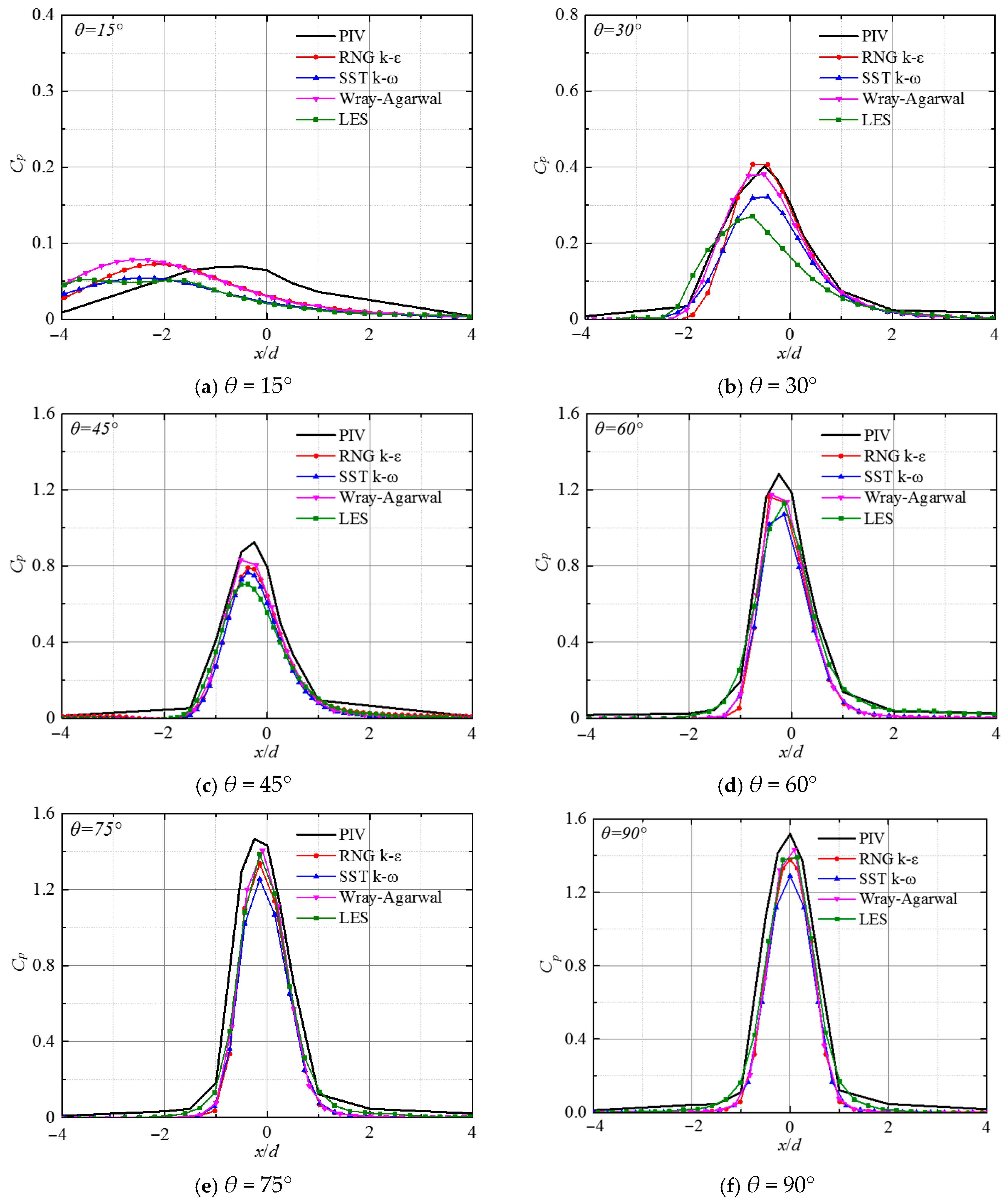
Figure 17 shows the distribution of pressure coefficient C_p along the x-axis on the impact plane for the submerged impinging jet at Re = 23,400 with H/d = 3 and impact angles of 15°, 30°, 45°, 60°, 75°, and 90°. C_p is defined as follows [21]:

$$C_p={\displaystyle \frac{P-P_{\infty }}{\frac{1}{2}\rho U_j^2}}$$

(1)

Figure 17. Pressure coefficient C_p along the x-axis for Re = 23,400, H/d = 3 at different impinging angles.

Here, P refers to the pressure at the investigated point, while P_∞ designates the ambient pressure.

The results of different numerical simulation schemes are basically consistent with the experimental values at the various impingement angles investigated in this study. At lower impinging angles, the predicted values of W-A and RNG k-ε turbulence models are the closest to the experimental values, which can effectively predict the distribution trend of pressure and accurately reflect the pressure changes near the wall surface. However, there is a certain positive deviation in the location where the maximum pressure occurs, with the peak pressure location showing a noticeable upstream shift compared to the experiment. As the impinging angle decreases, this phenomenon becomes more pronounced. This is primarily due to the transition of jet flow from axial to radial direction, resulting in intense momentum and energy exchange. With increment of impinging angle, the pressure distributions calculated by the LES method gradually approach the experimental measurements.

5. Conclusions

In this paper, the numerical calculation model of a submerged impinging jet under different impinging angles is established. The W-A and RNG k-ε, SST k-ω turbulence models of RANS and LES methods are used to simulate the submerged impinging jet. The numerical prediction results are compared with experimental data, validating the applicability of various turbulence models in predicting the flow field of submerged impinging jets. The following conclusions are obtained:

(1)

The results predicted by the RANS turbulence model and the LES method are in good agreement with the experimental observations, enabling the capture of flow field evolution trends and variation characteristics. In the free jet zone of the submerged impinging jet, predictions from the RANS turbulence model are in better agreement with the experimental data than those from LES. At small impinging angles, the LES method prematurely predicts the jet decay location; as the impact angle increases, the accuracy of LES predictions improves progressively. The prediction results of the SST k-ω turbulence model are significantly lower than the experimental values, showing less satisfactory performance than the W-A and RNG k-ε models. In general, the RNG k-ε and Wray-Agarwal models are strongly recommended for predicting the mean macroscopic flow field. Their advanced R_ε in RNG k-ε and the cross-diffusion term in WA effectively suppress the stagnation point anomaly and correctly predict the shear layer flow characteristic, offering an optimal balance of accuracy and computational efficiency.

(2)

In the wall-jet region, when the impact angle θ is relatively small, the one-equation W-A turbulence model exhibits the best performance, accurately capturing the range of the stagnation zone and its attenuation characteristics along the flow path. As the impinging angle increases, the RNG k-ε turbulence model, SST k-ω turbulence model, and LES methods perform better than the W-A turbulence model. Furthermore, as the wall jet evolves, these three sets of predictions align closely with the experimental data.

(3)

Overall, for submerged impinging jets, the LES method has lower predictive accuracy compared to RNG k-ε under the selected grid scheme in this study. However, as the impinging angle increases, the prediction results of both methods gradually converge. Furthermore, in the wall-jet region, the LES predictions agree more closely with experimental data. Therefore, while the LES approach demonstrates high fidelity in vertically impingement due to its accurate near-wall asymptotic behavior, extreme caution is advised when applying it to small-angle oblique impingement. The severe macroscopic asymmetry in oblique jets compromises the subgrid-scale isotropy assumption, necessitating impractically strict grid resolutions to maintain accuracy.

References

- Mao, J.; Si, J.H.; Chen, J.; Li, G.; Wang, X. Experimental investigation on sand bed scour by an oblique planar water jet at varying impinging angles. Ocean Eng. 2023, 279, 114526. [Google Scholar] [CrossRef] [Scilit]
- Wang, X.K.; Gong, K.; Liu, H.; Zhang, J.X.; Tan, S.K. Flow around four cylinders arranged in a square configuration. J. Fluids Struct. 2021, 43, 179–199. [Google Scholar] [CrossRef] [Scilit]
- Yu, H.; Wang, C. Efficiency and vortex dynamics of orifice pulsed jet propulsion based on large eddy simulation. Energy 2026, 344, 140098. [Google Scholar] [CrossRef] [Scilit]
- Jiang, B.; Wang, A.L.; Wang, J.H. Numerical simulation and experiment of breaking soil by jet under submerged condition based on ALE method. J. Chin. Agric. Mech. 2020, 41, 196–203. [Google Scholar] [CrossRef]
- Cooper, D.; Jackson, D.C.; Launder, B.E.; Liao, G.X. Impinging jet studies of turbulence model assessment-I. Flow-field experiments. Int. J. Heat Mass Transf. 1993, 36, 2675–2684. [Google Scholar] [CrossRef] [Scilit]
- Yu, H.; Zuo, Z.; Wang, C.; Li, G. Unsteady mechanisms of pulsed thermally buoyant jets for enhancing ventilation performance of indoor air supply outlets. Build Environ. 2026, 294, 114386. [Google Scholar] [CrossRef] [Scilit]
- Hosseinalipour, S.M.; Mujumdar, A.S. Comparative evaluation of different turbulence models for confined impinging and opposing jet flows. Numer. Heat Transf. Part A 1995, 28, 647–666. [Google Scholar] [CrossRef] [Scilit]
- Angioletti, M.; Nino, E.; Ruocco, G. CFD turbulent modelling of jet impingement and its validation by particle image velocimetry and mass transfer measurements. Int. J. Therm. Sci. 2005, 44, 349–356. [Google Scholar] [CrossRef] [Scilit]
- Huang, H.; Sun, T.; Li, N.; Zhang, G. Sensitization of the modified SST model to the swirling and curvature for turbulent impinging jet heat transfer. Int. J. Heat Mass Transf. 2022, 182, 121980. [Google Scholar] [CrossRef] [Scilit]
- Gohil, T.B.; Saha, A.K.; Muralidhar, K. Numerical study of instability mechanisms in a circular jet at low Reynolds numbers. Comput. Fluids 2012, 64, 1–18. [Google Scholar] [CrossRef] [Scilit]
- Mihaescu, M.; Semlitsch, B.; Fuchs, L.; Gutmark, E. Assessment of turbulence models for predicting coaxial jets relevant to turbofan engines. In Proceedings of the 15th International Conference on Fluid Flow Technologies, Budapest, Hungary, 4–7 September 2012; pp. 716–723. [Google Scholar]
- Xu, B.P.; Wen, J.X.; Volkov, K.N. Large-eddy simulation of vortical structures in a forced plane impinging jet. Eur. J. Mech. B-Fluids 2013, 42, 104–120. [Google Scholar] [CrossRef] [Scilit]
- Giralt, F.; Chia, C.J.; Trass, O. Characterization of the impingement region in an axisymmetric turbulent jet. Ind. Eng. Chem. Fundam. 1977, 16, 21–28. [Google Scholar] [CrossRef] [Scilit]
- Ragunathan, S. Numerical simulation of the flow field of a confined, submerged slot jet impinging on an oscillating surface: A parametric study. In Proceedings of the ASME 2016 Fluids Engineering Division Summer Meeting collocated with the ASME 2016 Heat Transfer Summer Conference and the ASME 2016 14th International Conference on Nanochannels, Microchannels, and Minichannels, Washington, DC, USA, 10–14 July 2016. Paper No: FEDSM2016-7743, V01AT03A016. [Google Scholar] [CrossRef] [Scilit]
- Guo, W.S.; Li, N.W.; Liu, C.; Li, L.G. Oblique submerged jets in the pool using les and k-ε turbulence model. J. Hydroelectr. Eng. 2020, 36, 7–15. [Google Scholar]
- Zhang, L.; Wang, C.; Zhang, Y.; Xiang, W.; He, Z.; Shi, W. Numerical study of coupled flow in blocking pulsed jet impinging on a rotating wall. J. Braz. Soc. Mech. Sci. Eng. 2021, 43, 508. [Google Scholar] [CrossRef] [Scilit]
- Zhang, Y.C.; Wang, C.; Chen, X.X.; Meng, W.X. Operation of oblique submerged jet impingement as impacted by impingement height. J. Irrig. Drain. Eng. 2020, 39, 71–77. [Google Scholar] [CrossRef]
- Chen, X.X.; Wang, C.; Shi, W.D.; Zhang, Y.C. Numerical simulation of submerged impinging water jet at different impact angles. J. Irrig. Drain. Eng. 2020, 38, 658–662. [Google Scholar]
- Han, X.; Rahman, M.; Agarwal, R.K. Development and application of wall-distance-free Wray-Agarwal turbulence model (WA2018). In Proceedings of the 2018 AIAA Aerospace Sciences Meeting, Kissimmee, FL, USA, 8–12 January 2018; p. 593. [Google Scholar] [CrossRef] [Scilit]
- Han, X.; Wray, T.; Agarwal, R.K. Application of a new DES model based on Wray Agarwal turbulence model for simulation of wall-bounded flows with separation. In Proceedings of the 47th AIAA Fluid Dynamics Conference, Denver, CO, USA, 5–9 June 2017; p. 3966. [Google Scholar] [CrossRef] [Scilit]
- Wang, C.; Wang, X.K.; Shi, W.D.; Lu, W.; Tan, S.K.; Zhou, L. Experimental investigation on impingement of a submerged circular water jet at varying impinging angles and Reynolds number. Exp. Therm. Fluid Sci. 2017, 89, 189–198. [Google Scholar] [CrossRef] [Scilit]
- Brazhenko, V.; Mochalin, I.; Cai, J.C. DIY-PIV system for Poiseuille flow investigation in undergraduate fluid mechanics course. Int. J. Mech. Eng. Educ. 2024, 53, 373–390. [Google Scholar] [CrossRef] [Scilit]
- Zhang, L.; Fan, J.; Wang, C.; Wang, Y.; Cui, Y. Numerical study on flow characteristics of a submerged circular water jet at varying impingement heights. Phys. Fluids 2025, 37, 025167. [Google Scholar] [CrossRef] [Scilit]
- Semlitsch, B.; Simic, S.; Cantrak, D.; Stojanovic, V.; Simonovic, J. Procedure for estimation and reporting of uncertainty due to discretization in CFD applications. J. Fluids Eng. 2008, 130, 078001. [Google Scholar] [CrossRef] [Scilit]
- Baurle, R.A.; Edwards, J.R. Hybrid Reynolds-averaged/large-eddy simulations of a coaxial supersonic free jet experiment. AIAA J. 2010, 48, 551–571. [Google Scholar] [CrossRef] [Scilit]
- Yakhot, V.; Orszag, S.A. Renormalization group analysis of turbulence. I. Basic theory. J. Sci. Comput. 1986, 1, 3–51. [Google Scholar] [CrossRef] [Scilit]
Disclaimer/Publisher’s Note: The statements, opinions and data contained in all publications are solely those of the individual author(s) and contributor(s) and not of MDPI and/or the editor(s). MDPI and/or the editor(s) disclaim responsibility for any injury to people or property resulting from any ideas, methods, instructions or products referred to in the content. |
© 2026 by the authors. Licensee MDPI, Basel, Switzerland. This article is an open access article distributed under the terms and conditions of the Creative Commons Attribution (CC BY) license.