


Abstract
A significant portion of Europe is prone to flooding, including severe events occurring over very small areas. Recent flood hazard mapping methods can cover large regions, but often fail to capture processes driven by small streams or direct rainfall. This study presents the authors’ experience in the application of a fully hydrodynamic model over an entire territory, with direct rainfall input (rain-on-grid approach at the basin scale). The case study is the Neto River basin in Calabria (Italy), covering approximately 1000 km2, a region that represents an ideal natural laboratory for investigating flash flood processes in Europe. Simulations were carried out using the TUFLOW 2D commercial modelling tool. A key objective is to demonstrate that the Chicago hyetograph enables a constant return period across the entire domain. Additionally, specific procedures are proposed to represent numerous minor crossings (e.g., small bridges, culverts, and road and railway underpasses) and dam outlets without refining the computational grid or abandoning the Shallow Water Equations (SWE). This approach allows identification of major river floods, flash floods, runoff-related hydraulic effects, and pluvial flooding. Results show that the fully hydrodynamic rain-on-grid model is highly effective for flood hazard mapping, with strong agreement between simulations and observed events, confirming its predictive reliability and enabling high-resolution, comprehensive territorial analysis.
1. Introduction
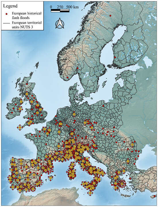
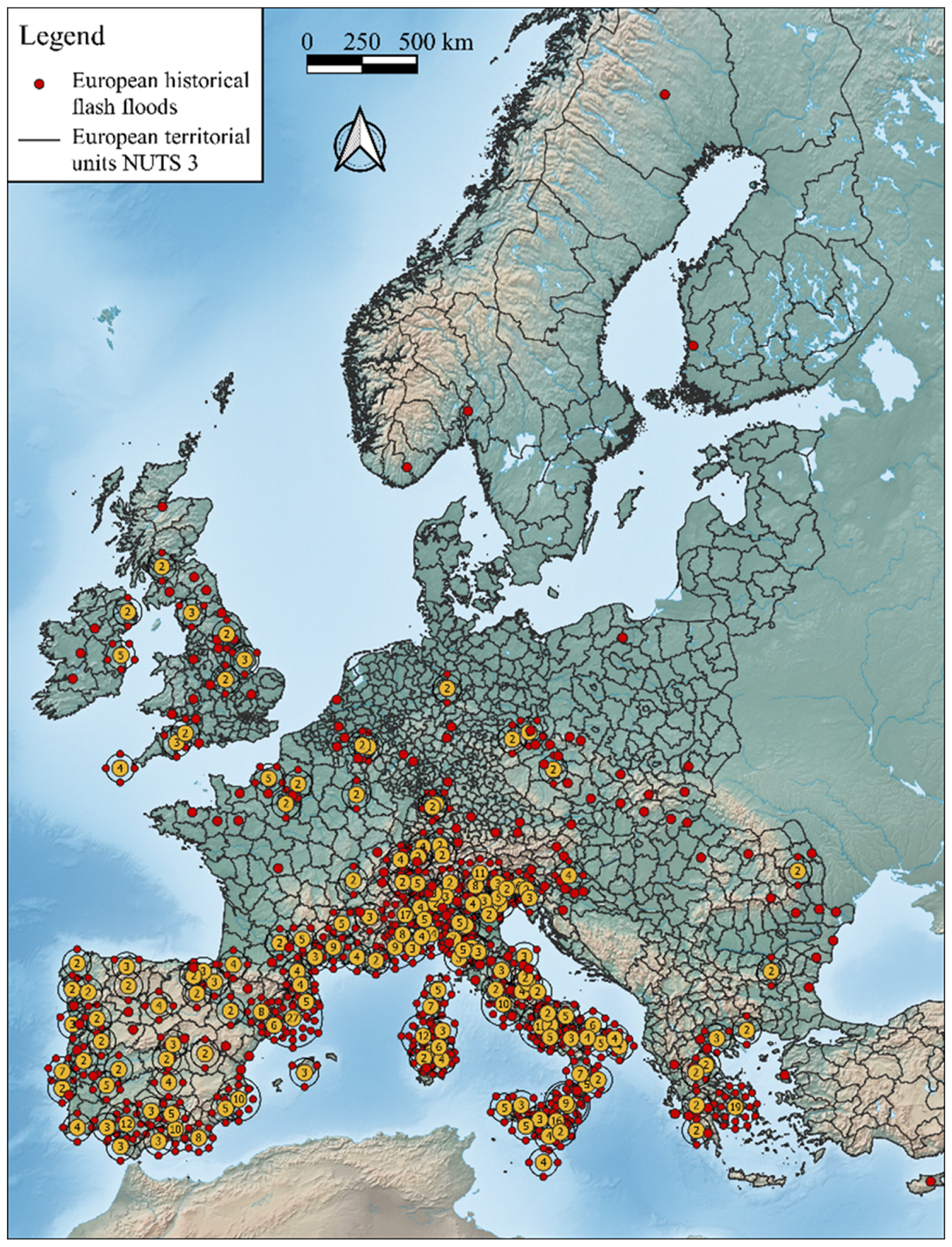
Over the past 150 years, 56% of flood events in Europe have been classified as flash floods [1,2,3,4]. Gaume et al. [5] include in flash floods those floods that occur in basins with an area of up to approximately 500 km2. They analyzed the Mediterranean regions of Spain, France, the Italian Alps and Liguria, Greece, and the Inland Continental regions of Slovakia, Romania, and Austria. Paprotny et al. [3] identified Italy, Spain, Portugal, France, Greece, Switzerland, Ireland, Great Britain, and Belgium as the countries where flash floods are more prevalent than other types of floods. Figure 1 illustrates the spatial distribution of flash floods in Europe, as recorded in the HANZE database [6], with data aggregated at the provincial level.
Figure 1.
Spatial distribution of flash floods in Europe from 1870 to 2016. The data are aggregated at the provincial territorial level. Each red point corresponds to a flash flood event that occurred within the province. In the provinces where more events occurred, the number of events is indicated in the yellow circle and by the number of red satellites surrounding the yellow circles (data derived from the HANZE database [6]).
In late October 2024, flash floods devastated the Valencia region of eastern Spain [7]. In some places, one year’s worth of rain fell in a few hours. More than 220 people have died [8]. In July 2021, extremely heavy rainfall caused devastating floods in Belgium, Germany, Luxembourg, and the Netherlands; more than 230 people died, and more than 750 people were injured [9,10]. A few days after the July 2021 floods that occurred in Europe, Science published an article titled “Europe’s deadly floods leave scientists stunned. Despite improvements, flood forecasts sometimes failed to flag risks along smaller streams” [11]. River floods are one of the most frequent natural disasters, and their risk is expected to rise in the future due to climate and socioeconomic changes [12,13].
Indeed, in recent years, numerical models capable of covering large areas have been proposed for flood hazard mapping at the continental level [13,14,15,16,17,18]. They are essentially composed of the coupling of a hydrological model that provides the forcing and a hydraulic routing model along the branches of the hydrographic network [19,20]. These models necessarily use grids with very large calculation cells, which makes it difficult to capture the network’s lower-order streams. One approach is to further detail the hydrographic network by adding lower-order (i.e., smaller) streams [21] and improving the detail of the hydrological forcing [22]. However, the hydrological–hydraulic coupling remains weak, as runoff is conceptually calculated, even when the areas considered are highly subdivided. Consequently, the approach should not be viewed as devoid of rigidity or limitations. Among these limitations, those related to the hydrological input required for a hydrodynamic model are significant. The challenge is to maintain a consistent return period across the entire hydrographic network to generate a map for the assigned return period in performing hydraulic simulations over large areas. The hydrological–hydraulic cascade approach is labor-intensive. For example, Alfieri et al. [13] and Dottori et al. [14] calculate the peak discharge with a fixed return period for each river pixel, along with the corresponding flood hydrograph, and use this input to run a 2D simulation along the hydrographic network. Sampson et al. [15], Wing et al. [16], and Wing et al. [17] employ a regionalized flood frequency analysis as hydrological input to feed the LISFLOOD-FP model for flood mapping. More recently, Wing et al. [17] have included a list of works that deal with global models, and among these, only one [15] also includes pluvial floods. Pluvial floods are also addressed by Wing et al. [17], who use intensity-duration-frequency (IDF) curves for a given return period as input for flood propagation models.
Despite these efforts in the hydrological–hydraulic cascade approach, issues regarding the treatment of the lag time of the hydrological inputs and the overlap of hydraulic effects between the studied reach and its tributaries remain open. Furthermore, the hydraulic effects of runoff and the resulting rainfall-induced flooding (i.e., pluvial floods) are entirely neglected or juxtaposed to fluvial floods.
In reality, floods are a unified hydrodynamic phenomenon affecting the entire basin, often generating the aforementioned effects in a combined manner. Therefore, this work proposes applying a complete hydrodynamic model across the entire basin simultaneously, with direct rainfall input (complete rain-on-grid hydrodynamic approach at the basin scale). With this approach, there is no need to rely on any pre-designed hydrographic network. Indeed, it is the calculation outcome that, in a consistent manner with the terrain morphology, will identify the paths of the hydrographic network, from the main streams up to the smallest mountain gullies. At the same time, the calculation will be able to identify the hydraulic effects of the runoff and all the rain-induced flooding.
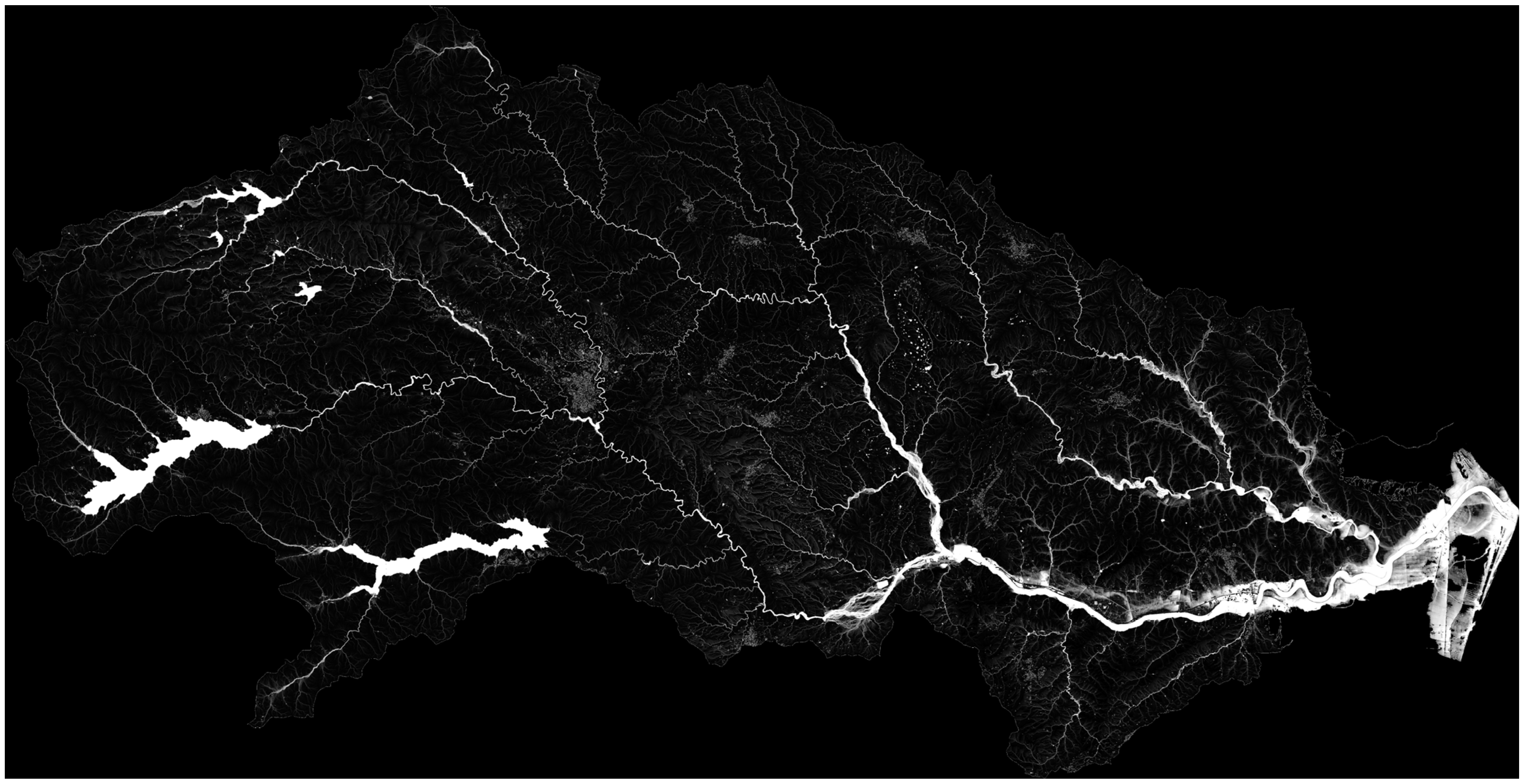
This way of conducting flood risk analyses provides hydraulic engineering with an advancement in diagnostics similar to the progress that occurred in medicine with the transition from radiography to contrast-enhanced computed tomography. In fact, with radiography, the investigation is focused on a specific point where a symptom is already present. Conversely, a full-body contrast-enhanced scan provides a much more powerful tool, detecting all parts of the body, including those where risk hotspots remain asymptomatic. In the rain-on-grid approach, the contrast medium is the stormwater. As will be clearly illustrated in a figure later in the paper, the numerical simulation of all possible stormwater paths generates a comprehensive image of the entire territory.
This includes the hydrographic network layout derived from the calculations, as well as stream overflows, runoff paths, and flooding areas. This represents a significant step forward in developing a diagnostic tool capable of covering the entire territory.
This approach is now gaining traction in the literature [23,24,25,26]. Several developments in numerical modelling—most notably recent enhancements to the LISFLOOD-FP code [27]—have enabled the implementation of rain-on-grid simulations at the basin scale. These updates have been suggested both for the approximate equations (diffusive or local inertial scheme) [28] and the complete equations [29]. Certainly, for the evaluation of hazard parameters when modelling very rapid events such as flash floods, which have durations of only a few hours and very high flow discharges, high flow velocities and short response times make inertial terms non-negligible. Therefore, complete equations must be used [24,30,31].
Although this approach has been traditionally applied to reconstruct events that occurred in individual basins [23,24,25,29,31], recent studies have begun to explore its suitability for broader, basin-scale flood-hazard assessments [32]. This growing interest is also driven by the potential of rain-on-grid models to represent spatially variable rainfall more realistically than traditional discharge-driven approaches.
It is important to note, however, that rain-on-grid simulations are generally more computationally demanding than conventional flood-modelling methods, as they require solving hydrodynamic equations over large domains while handling spatially distributed rainfall inputs and detailed topographic datasets. These factors typically result in higher numerical complexity and longer computational times. Nonetheless, this computational burden can be substantially reduced by leveraging high-performance computing (HPC) architectures, including multi-GPU frameworks specifically developed for large-domain hydrodynamic modelling [33,34].
This work presents the authors’ experience in the use of the complete rain-on-grid hydrodynamic model at a large scale for hazard mapping. In this context, to capture hydraulic phenomena at all points of the territory, it is necessary to achieve the level of detail typically used in local studies (an interesting example of a hyper-resolution coupled hydrological–hydraulic model applied to the territory of Austria can be found in Blöschl et al. [35]). To this end, it is necessary to have a high-resolution topographic representation. Additionally, structures that interfere with the flow must be included in the calculation domains. Furthermore, generating maps for assigned return periods presents a challenge, even with this method. The key difficulty is incorporating rainfall input in a way that ensures a spatially consistent distribution of hydrodynamic quantities with a uniform return period. In this regard, this study shows both theoretically and numerically that the Chicago hyetograph enables the determination of the critical peak flow rate while ensuring the constancy of the return period at any cross-section within the hydrographic network using a single simulation. Therefore, this work shows a procedure that can be applied at a large scale for full-coverage mapping of the territory in the context of European areas prone to flash and pluvial floods. In this context, the Calabria region (Italy), located at the southern tip of the Italian peninsula, serves as an ideal natural laboratory representative of European areas where flash floods occur [36,37].
The motivation for this study and its main challenges, objectives, and expected results can be summarized as follows:
Study motivation
- Need for large-scale hazard mapping capable of capturing detailed hydraulic processes across the entire territory.
- Requirement to achieve a level of detail comparable to that of local-scale studies.
- Challenges in ensuring consistent hydrodynamic outputs (e.g., return periods) over large computational domains.
Methodological challenges
- Necessity of high-resolution topographic data.
- Inclusion of flow-interfering structures within the computational domain.
- Difficulty in generating hazard maps for assigned return periods using rain-on-grid models.
- Need to ensure spatial consistency of rainfall input and related hydrodynamic variables.
Study objectives
- Apply a complete rain-on-grid hydrodynamic model at a large scale.
- Develop a criterion to identify the critical peak flow rate.
- Ensure a uniform return period across all cross-sections of the hydrographic network within a single simulation.
Expected contribution
- Provide a scalable procedure for full-coverage hazard mapping.
- Support flood risk assessment in European regions prone to flash and pluvial floods.
This article presents the results of the aforementioned methodology, implemented with the TUFLOW 2D commercial modelling tool, for a sample area of approximately 1000 km2, which coincides with the Neto River basin (Calabria, Italy). As will be further specified in the next paragraph, this area is characterized by sub-basins of limited size. Furthermore, there are several dams for which this article shows a treatment criterion to account for the attenuation effect of downstream flood peaks.
2. Materials and Methods
2.1. Rain-on-Grid Full Hydrodynamic Approach
Two-dimensional hydraulic modeling has advanced significantly in recent years and today provides powerful and flexible tools capable of supporting flood risk analysis. There is a wide variety of shallow-water equations (SWE) based codes characterized by various levels of physical simplification. However, simulating rapidly evolving phenomena such as flash floods necessarily requires the use of codes based on the complete SWE equations, written in conservative form [38]:
where h (m) is the water depth, t (s) is the time, u (m/s) is the velocity in the x direction, v (m/s) is the velocity in the y direction, g (m2/s) is the gravitational constant, z (m a.s.l.) is the bed elevation, and Sfx and Sfy (-) are the frictional resistances in the x and y directions, respectively. The x and y directions refer to the Cartesian spatial coordinate system, expressed in meters (m).
The terms Sfx and Sfy are calculated using the Manning equation:
where n (s/m1/3) is the Manning’s roughness coefficient. The presence of rainfall intensity R (m/s) and infiltration rate I (m/s) in the continuity equation allows the application of the rain-on-grid approach. To apply these equations in this study, which aimed at analyzing large areas, it was necessary to choose a robust, accurate computational code capable of preserving all the topographic information provided by high-resolution LiDAR data. A selection of validated computational codes from the literature was reviewed. The chosen model was the HPC GPU (High-Performance Computing, Graphics Processing Unit) version of the TUFLOW 2D hydrodynamic model [39]. The code uses a second-order accurate finite volume explicit scheme in space and a fourth-order scheme in time for integrating the SWEs, with an adaptive time step.
2.2. Rainfall Input
Given the lack of historical data on flood discharges, the guidelines of the Calabria Region suggest estimating flood discharges using indirect methods, by resorting to the “statistical analysis of rainfall observations related to the watershed upstream of the section of interest.”
The guidelines assume, for catchments with an area smaller than approximately 250 km2, “that extreme flood events occur under conditions of nearly saturated soil, due to previous rainfall, and that such conditions are homogeneous across the entire basin, given its limited size.”
With regard to estimating discharges at a given cross-section of the watercourse, the guidelines refer to the rational method approach. Therefore, the criterion for selecting the rainfall input used in this study, following the procedures indicated by the guidelines, was inspired by the principles of the rational method, which assumes that the estimated flow rate has the same return period T as the rainfall intensity. Moreover, as is well known, this method requires assuming the critical rainfall event for each basin under study. This is identified as the event caused by rainfall with a duration equal to the basin’s time of concentration.
This presents a problem since using rainfall intensity corresponding to each basin’s time of concentration as input in the hydrodynamic model would, in theory, require an infinite number of simulations. This is because, as one moves downstream along the main channel, the cross-sections encompass increasingly larger basins, and the time of concentration increases accordingly. However, computational efficiency necessitates minimizing the number of simulations.
This represented the main challenge of using the rain-on-grid approach at the basin scale for predictive purposes and remains a critical issue for those seeking to apply this method over large areas.
The central idea was to use the Chicago hyetograph as the rainfall input [40,41]. As will be demonstrated below, this approach enables the determination of the critical peak flow rate, ensuring the constancy of the return period at any cross-section within the hydrographic network using a single simulation.
The Chicago hyetograph allows the calculation of the critical flow for each point of the basin’s hydrographic network: demonstration.
As regards the hyetograph, we refer here to the Chicago hyetograph, proposed by Keifer and Chu [42] and, in particular, to the “Complete Advanced Storm pattern” (CASp) hyetograph, which can be written in the following form:
in which and aT are the numerical constants of the cumulative distribution function. Specifically, aT depends on the return period.
This hyetograph has the property of having, for td = tc, the same average intensity as given by the intensity–duration–frequency (IDF) curve.
The well-known rational method ([43]; Equation (7)) states that the value of the critical flow is proportional to a constant rainfall intensity (itc,T) multiplied by the surface area of the catchment (A) and by the runoff coefficient (φ), which accounts for water losses:
where itc,T is evaluated for td = tc (which is the critical event duration, since tc can be seen as the time required for the entire drainage area of the basin or sub-basin to contribute to the runoff; see [44,45]) and for a given value of T.
Assuming a linear rainfall excess-runoff model, the hydrograph for a specific value of T [i.e., QT(t)] can be expressed as the sum of the infinitesimal runoff values dQT(t) = in,T(τ)dA(t − τ):
where in0,T(τ) is the net rainfall intensity for a specific value of T, dA(t − τ) is an infinitesimal area of the basin that contributes to the runoff at time t, and τ is a dummy variable in terms of time that accounts for the time needed to reach the basin closing section from the centroid of the infinitesimal area dA, while A(t) is the total area contributing to the runoff at time t.
This paragraph shows that the application of the CASp hydrograph as rainfall input in the hydrodynamic model allows the calculation of the critical flow for each point of the hydrographic network of the basin. This method eliminates the need to perform separate simulations for each section of interest. Traditionally, each section requires adjusting the time of concentration, which in turn alters the critical rainfall intensity used in calculations. Instead, by running a single simulation using the CASp hydrograph across the entire basin, the critical flow at each section can be determined effectively, replicating the results that would be obtained using the rational method.
Initially, consider an ideal basin with a rectangular shape, constant longitudinal slope, and zero transverse slope (i.e., a flat inclined plane). Since the time required to reach the outlet is proportional to the length of the path of each water particle, and the length is proportional to the elevation difference between the position of the infinitesimal area dA and the closing section [46], A(t) can be considered coincident with the hypsometric curve of the basin or sub-basin. Considering a rectangular plane as the ideal basin with constant slope and roughness, A(t), for t ≤ tc follows a linear law for each sub-basin, that is, A(t) = At/tc, where tc refers to the considered basin or sub-basin. Therefore, dA(t − τ)/dτ = A/tc and dA(t − τ) = (A/tc)dτ, while Equation (10) becomes the following:
According to Pilgrim and Cordery [44] and Merz et al. [47], φ can be expressed as the ratio between the volume of rainfall (or depth) that becomes runoff, i.e., the net volume of rainfall (or depth), and the total volume of rainfall (or depth) occurring at t = td. Therefore, in0,T(t) can be rewritten as in0,T(td) for t = td, where in0,T(td) is the total rainfall intensity expressed as CASp (i.e., =aTn0td(n0−1)). Consequently, in0,T(td) = φaTn0td(n0−1), while QT(t) = QT(td) = QCASp,T(td):
For a critical duration (i.e., td = tc), Equation (10) returns, for the basin and sub-basins, the critical peak flow discharge value obtained with the application of the rational method [Equation (7)], that is, QRF,T:
For a (ideal) rectangular basin, it is thus demonstrated that the use of the descending Chicago-type hyetograph allows the calculation of the peak flow discharge value in each section of the watercourse, which would be obtained by applying the rational formula.
Actually, the area–time curve is not linear in real basins. Therefore, in Appendix A, an analysis is presented on some basins in Calabria to verify the degree of agreement between the peak flow calculated with the descending Chicago hyetograph and the one calculated using the rational formula. It can be easily demonstrated that the equality of peak flow values using the rational formula also holds for all other possible variants of the Chicago hyetograph. In Appendix A, the reasons for choosing the CASp in this study will be provided.
2.3. Computational Domain Setup
The computational domain is represented by a structured Cartesian grid with square cells. The code uses a sub-grid treatment to preserve all available topographic information. The following specific procedures are proposed to represent numerous minor crossings (e.g., small bridges, culverts, and road and railway underpasses) and dam outlets without refining the computational grid or abandoning the shallow water equations (SWEs).
2.3.1. Minor Crossings
The LiDAR survey is usually not cleared of the footprints of minor bridges, culverts, and underpasses of road and railway embankments. As a result, it may happen that flooded areas are overestimated on the upstream side and underestimated on the downstream side. On the other hand, these structures are smaller than the grid cells used for large-area computations. Local refinement of the grid would lead to a significant increase in computation times and the computational grid setup burden, considering the large number of structures.
Therefore, it is useful to adopt fast treatment strategies that, without the need to describe in detail the geometry of the crossing, are able to correctly simulate the hydraulic phenomenon at the spatial scale of interest for the study, which is the territorial scale.
For this reason, a rapid technique has been applied that involves adding openings in the computational domain, at the locations of crossings, with a width equal to twice the width of the grid cell. The grid cells falling within these openings are then penalized with a reduction factor, which is taken into account in the flux calculation to simulate the hydraulic effect corresponding to the actual dimensions of the structures. The geometric parameters of the hydraulic structures were obtained from available technical and official sources; where data were unavailable, they were reconstructed through desk-based research. Further details on this technique and its performance can be found in [40].
2.3.2. Large Dams and Reservoirs
Large dams and reservoirs influence the dynamics of floods due to the attenuation effect of the peak of the flow hydrographs entering the reservoir. The most unfavourable situation that can be hypothesized is that of the reservoir full up to the spillway overflow level. Similarly to the problem of minor crossings that interfere with flood waters, a method has also been developed to deal with the presence of dams that avoids having to deal in detail with the hydraulic phenomenon that occurs through the spillway. This would require a specific study and the application of hydraulic laws that cannot be traced back to gradually varied flows.
The identified method allows for the treatment of the effect of the presence of the reservoir without suspending the application of the SWE. To this end, the initial water surface within the reservoir was assumed to be the one located at the spillway overflow level. Furthermore, in correspondence with the dam body, an exit chute was introduced, with a rectangular section, whose base, at the inlet of the chute, is located at the level of the aforementioned horizontal surface and whose downstream end is located at the riverbed downstream of the dam. A constant slope was assigned to the chute of a value, such as to make the SWE legitimately applicable. With the introduction of such a chute, the flow at the beginning of the channel is characterized by the passage through the critical state. Therefore, the presence of the chute is equivalent to the presence of a broad-crested weir acting as a spillway. Indeed, it is known that spillways are generally made with a Creager-type sill profile, which has a discharge coefficient of approximately 0.48, which is significantly higher than that of the broad-crested weir, which is 0.385. To take this into account, the chute was assigned a cross-section width equal to 1.25 times the sill width of the spillway. This factor derives from the ratio between the discharge coefficient of the Creager profile and that of the broad-crested weir. For spillways controlled by gates, the initial surface of the reservoir was always placed at the maximum regulation level, but the instantaneous opening of the gate was assumed.
2.3.3. Levees
Finally, some watercourses in the region are bordered by levees. To accurately represent these structures, the sub-grid sampling (SGS) module was activated during the simulations with the TUFLOW model. This allowed the preservation of all original topographic information at a resolution of one point per square meter. Thanks to this approach, levees smaller than the computational cell size were also properly taken into account.
2.4. Output
The model output consists of maps, for a given return period, of water depth (h), velocity (V), and the product Vh for each computational cell, enabling the identification of channelized flows and their overflows, as well as pluvial flooding with complete land coverage.
2.5. Workflow
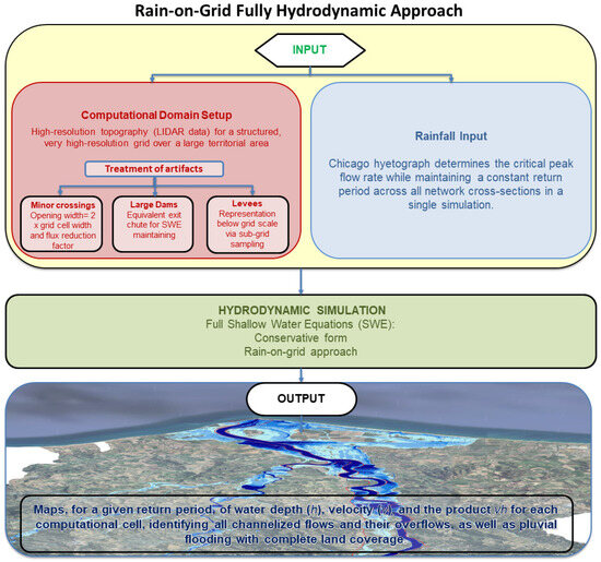
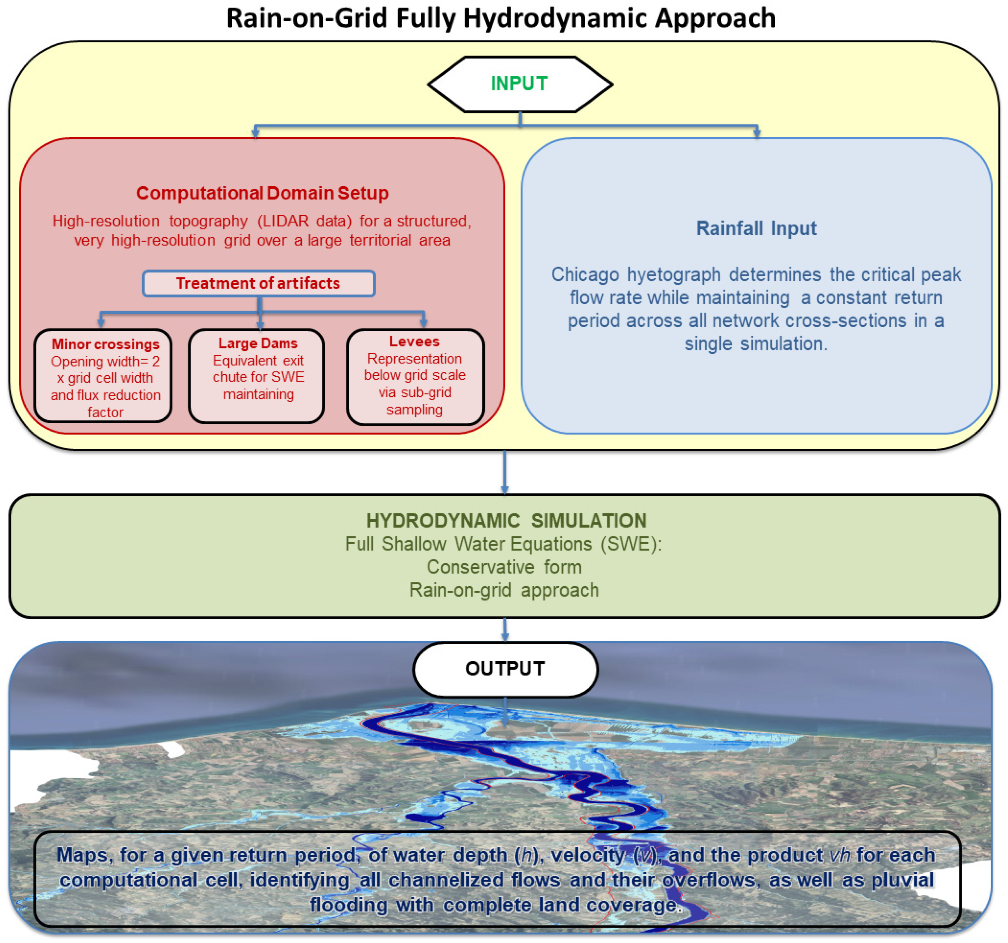
For clarity, the procedure described in this section is schematically represented in the workflow shown in Figure 2.
Figure 2.
Workflow of the procedure illustrated in Section 2.
3. Case Study
3.1. Characteristics of the Study Area
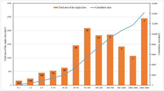
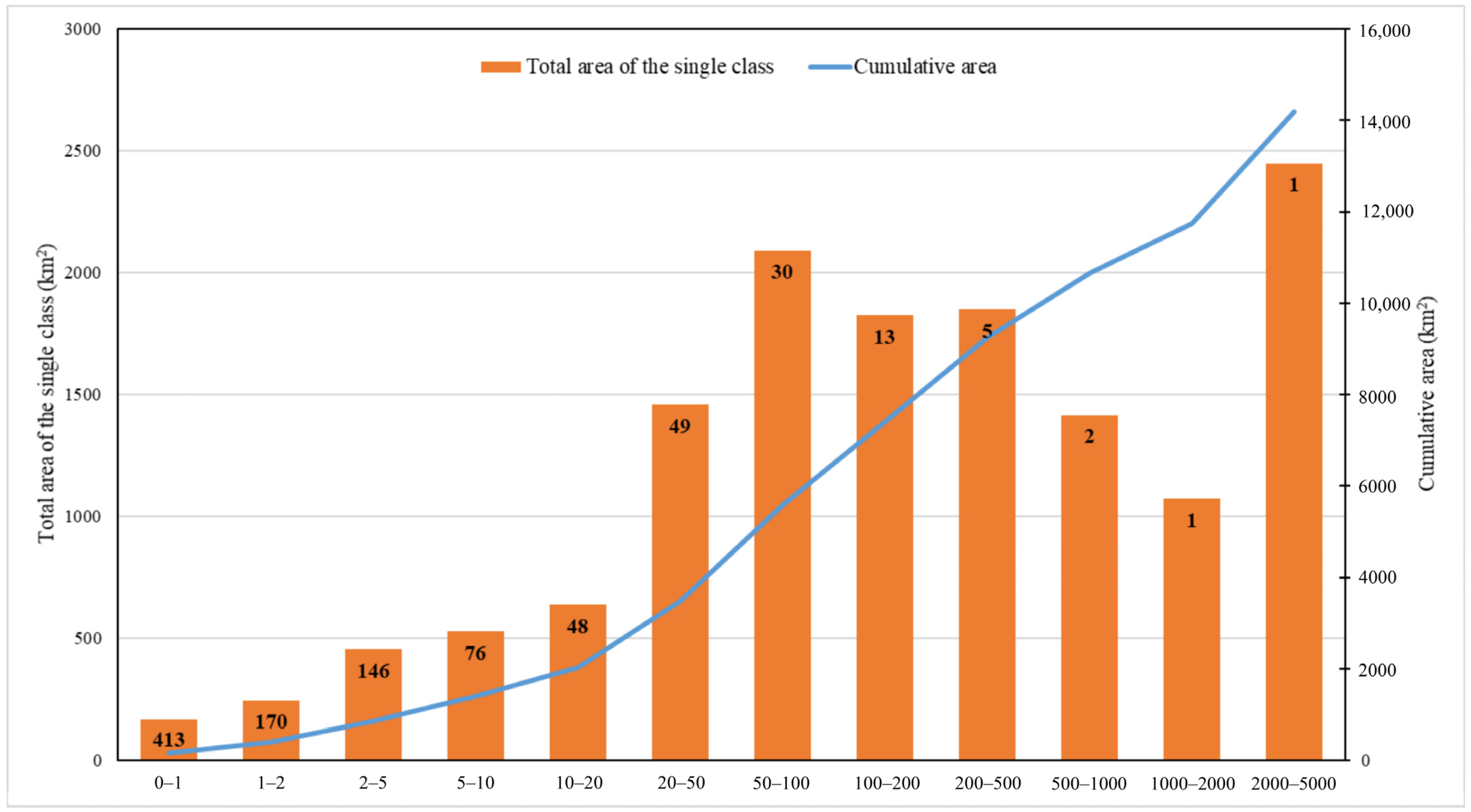
The study area is located in the Calabria region (Italy). The region’s morphology is predominantly mountainous and hilly. Its rivers exhibit a torrential regime. The territory is divided into 1003 basins that flow into the sea. Of these, only four basins have an area larger than 500 km2 (see Figure 3).
Figure 3.
Distribution of the basins in Calabria (Italy). On the x-axis, the classes of basin areas in km2; on the left vertical axis, the total area of the basins in a given class. On the right vertical axis, the cumulative area of the basins with an area equal to or smaller than the upper limit of a given class. The total number of basins belonging to each class is indicated in the bars of each class.
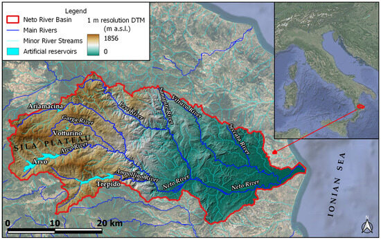
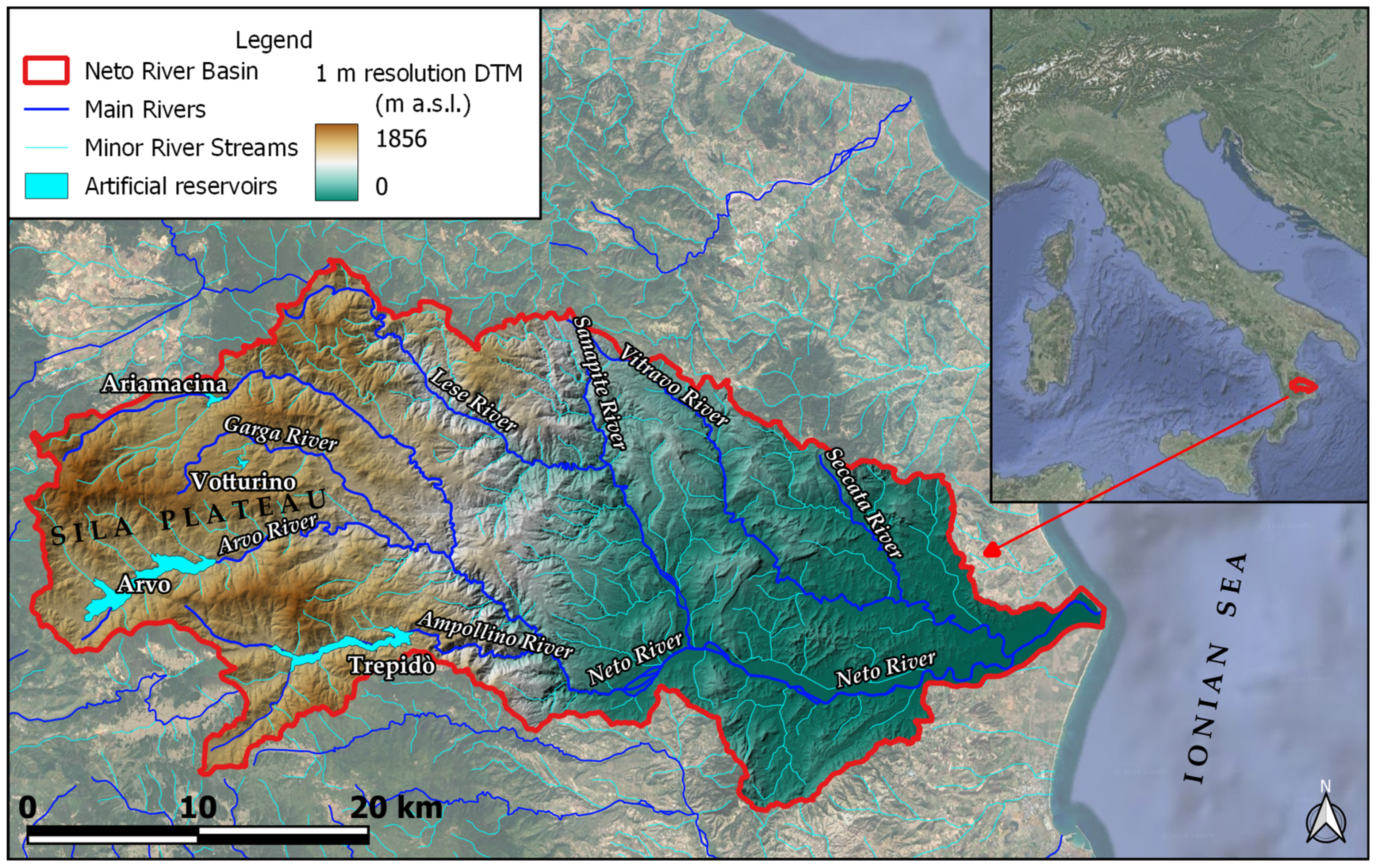
The area examined here covers an area of approximately 1073 km2 and coincides with the Neto River basin. The maximum altitude is approximately 1856 m above sea level. The average altitude is around 824 m above sea level. The average gradient is estimated at approximately 25.30%. The area, therefore, presents considerable altitudinal variability: from the mountain peaks of the Sila plateau to the coastal area of the Ionian Sea. The overall hydrographic network in the area is quite dense, with approximately 847 km of watercourses and several small and very small basins. Table 1 shows the division of the area into 9 sub-basins. Figure 4 shows the study area, its geographical location, topography, and the drainage network.
Table 1.
Main sub-basins within the study area and their areal extent.
Figure 4.
Study area, its geographical location, topography, and drainage network.
It is important to note that the hydrodynamic analysis method proposed in this study does not require the prior identification of the sub-basins. The purpose of the table is to highlight the small spatial extent of the sub-basins.
In this area, annual rainfall typically varies between approximately 760–1440 mm/year, with most precipitation concentrated in the autumn and winter months (October to March), while summer is characterized by low rainfall [48].
The watercourses typically have a torrential flow regime: in summer, very low flow (low water), and in winter or during heavy rainfall, violent floods [49].
The torrential nature of the watercourses, combined with the geomorphological conformation (steep slopes in the mountainous areas, alluvial fans in the plains, and a widened riverbed downstream), makes the valley portion of the Neto River susceptible to flooding. The Neto River basin includes several artificial reservoirs created by damming its tributaries.
In the area examined here, there are five artificial reservoirs, listed in Table 2, which reports some quantitative information.
Table 2.
Artificial reservoirs present in the study area.
3.2. Hydrodynamic Model Setup and Input Data
The calculations were carried out using a hyper-resolution structured grid of cells with dimensions of 5 m × 5 m. For the topography data, LiDAR surveys conducted in 2009 by the Italian Ministry of the Environment were used; available at: https://sim.mase.gov.it/portalediaccesso/mappe/?#/viewer/new, accessed on 7 March 2022. The surveys provided a resolution of 1 point per m2 for inland areas and 1 point per 4 m2 for coastal areas.
Simulations were performed on a structured computational grid, with the computational domain discretized into approximately 45 million cells.
The simulation started from dry initial conditions. Wetting and drying processes were activated using threshold depths of 0.002 m for cells and 0.001 m for cell sides, allowing dynamic representation of floodplain inundation.
Boundary conditions were implemented through an external boundary condition database linked to GIS layers. Rainfall inputs were applied as spatially distributed and temporally stepped boundary conditions.
Bed resistance was represented using a uniform Manning’s roughness coefficient equal to 0.05 s·m−1/3. The adoption of a uniform Manning’s roughness coefficient was supported by previous applications in similar basins within the study region, where the same value allowed a satisfactory reproduction of observed flood extents [50].
The numerical solution employed an adaptive time step based on the Courant–Friedrichs–Lewy condition.
Model outputs, including water depth, flow velocity, and water surface elevation, were recorded at 10 min intervals and stored in XMDF and ASCII grid formats. In addition, maximum values over the entire simulation period were extracted for subsequent analysis.
IDF Curves Used in the Study
First, the authors derived the maximum volume of water falling during the event from the intensity–duration–frequency (IDF) curve selected for a specific return period, T, value, considering the duration of the rain (i.e., td) equal to the concentration time, tc. The IDF curves suggested by the Calabria region guidelines were used [51]. They were derived from a regional-scale analysis. In particular, the third level of regionalization was used, where estimates of the mean value of the maximum annual rainfall for different durations at ungauged sites are achieved using regression models. A distributed rainfall input, made with 25 m × 25 m rain cells, was used in the hydrodynamic model calculations. Net rainfall was calculated for each cell using the SCS–CN (soil conservation service–curve number) approach [52]. The hyetograph was constructed on an hourly basis. For the choice of the curve number, CN, variable between 0 and 100 and tabulated by the SCS according to the land’s runoff capacity and the land use, the antecedent moisture conditions (AMCs) were considered, as a precaution, to be humid (i.e., AMC of type III, according to the classification of the SCS tabulations). The regional CN map was created based on the information provided by the soil infiltration map and the CORINE land use project map (https://portalecartografico.regione.calabria.it/dataset/pgra-piano-gestione-rischio-alluvioni; https://www.isprambiente.gov.it/it/attivita/suolo-e-territorio/suolo/copertura-del-suolo/corine-land-cover, accessed on 21 March 2022).
4. Results and Discussion
4.1. Simulation Execution and Results
This section presents the results obtained from the procedure described above for mapping the flood hazard in the study area for a 100-year return period. Rainfall inputs with the same return period, corrected to obtain net rainfall according to the procedure outlined earlier, were used. The simulation required a computation time of 18 h.
Before presenting the maps, it may be of interest to show the results of the proposed procedure for accounting for the influence of dams on flood dynamics.
The accuracy of the simulation of the attenuation effect obtained with the procedure described above was assessed by comparing the results with those obtained through the local hydraulic analysis of the attenuation effect. This analysis was performed by integrating the continuity equation applied to the reservoir volume. To describe the reservoir morphology, the height–volume curve was obtained from the available design data. The equation was integrated by inserting the inlet flows calculated with the hydrodynamic model. To calculate the outlet flow rate from the spillway, the outflow law was used with the discharge coefficient typical for the Creager profile (0.48) and with the overflow threshold width equal to the design one. The outlet hydrograph was calculated by integrating the continuity equation.
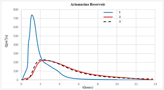
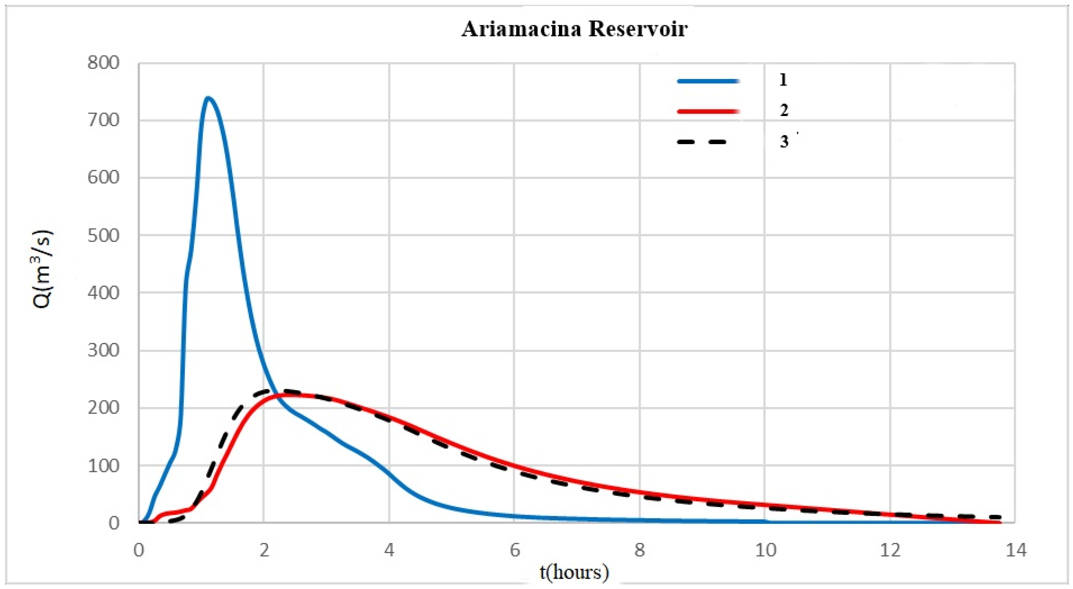
The results obtained in this way practically coincide with those provided by the hydrodynamic model. As an example, Figure 5 shows the results obtained for the Aramacina reservoir.
Figure 5.
Comparison between the results obtained with the procedure described in Section 2.3.2 (red line, 2) and with the integration of the continuity equation (dashed black line, 3) using as input the inlet hydrograph shown in the figure (blue line, 1).
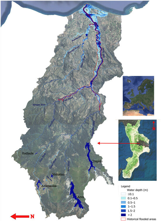
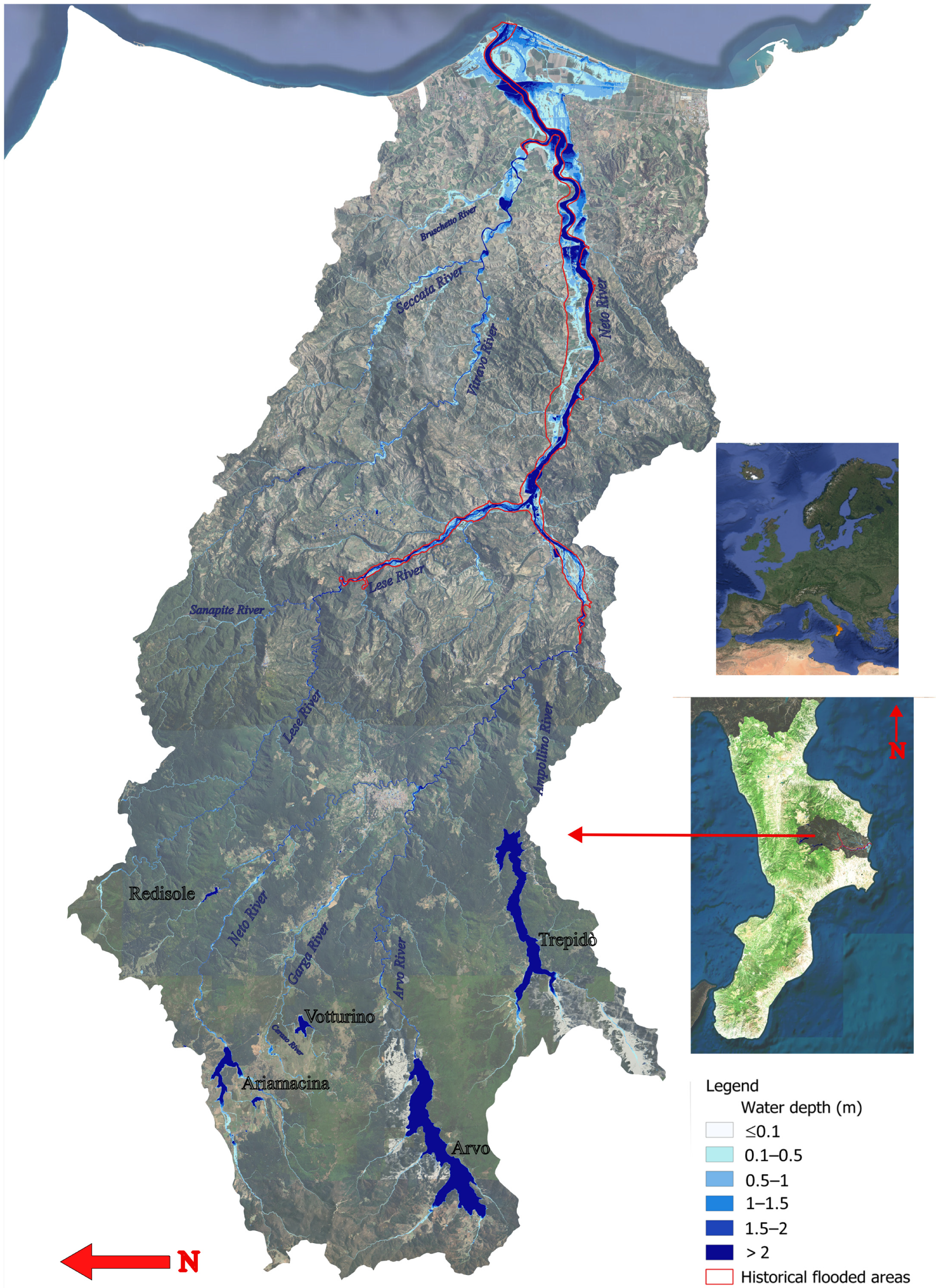
Figure 6 illustrates the mapping obtained using this methodology for T = 100 years, where areas outlined in red indicate historically flooded zones.
Figure 6.
Maximum water depth map of the study area. The map was obtained using the full rain-on-grid hydrodynamic model for T = 100 years; the red outlines are the documented historical flooded areas.
A standard criterion for evaluating hydraulic result reliability is comparing computed peak discharges with those derived from statistical analysis of historical data. Unfortunately, Calabria in general and, in particular, the basin examined here lack sufficient historical extreme flow data, making this approach practically unfeasible [51].
However, it should be noted that the objective of this study is not hydrological but to estimate the hydraulic effects of rainfall on the flood-prone areas. Thus, the reliability of the results can be effectively evaluated by verifying whether the simulated areas correspond to areas that have historically experienced flooding.
For this purpose, the simulation results were compared with the historical flooded areas available for the study area (the historical flooded areas were taken from the website https://portalecartografico.regione.calabria.it/dataset/pgra-piano-gestione-rischio-alluvioni, accessed on 30 June 2025). The return period of these flood events is unknown. For this reason, the comparison was made using multiple return times.
The results of this comparison are reported in the following subsection.
4.2. Validation and Discussion of Results
The authors validated the results by confirming that the historically flooded areas were included among those identified in the study. To assess the quality of the overlap, a visual analysis of the results is more than sufficient (see Figure 6). However, for a quantitative evaluation, typically, the comparison between a modeled flooded area (M) and an observed or historical flooded area (R) is performed using the Jaccard Index (0 ≤ J ≤ 1):
This index measures the overlap between the simulated and actual flooded areas relative to their combined extent [53]. It is clear that, while the historical map only shows the contours of the flooded area caused by a single event of a single watercourse, in the map for a given return period, all the events that can occur at any point in the territory are simultaneously reported. Another aspect to consider is that the historically flooded areas are those due to river flooding only, while the mapping also includes the areas affected by flooding from rain.
For this reason, it is not possible to extract from the map the value of M to compare with the historical case. To overcome this difficulty, the comparison between the historical flooded areas and the map has been limited to the areas included in the delimitation of the historically flooded areas.
Therefore, the previous index has been simplified as follows:
which simply expresses the proportion of the historical flooded area that coincides with the model prediction.
A further problem arises in the choice of the map to be compared, since they vary with the return period, and, unfortunately, the return periods of historical events are not known. In this situation of uncertainty, the authors decided to compare the historical flooded areas with the maps relating to multiple return periods.
Table 3 provides the flooded area values calculated for each zone for return periods of 50, 100, 200, and 500 years, which correspond to the reference return periods adopted in the Italian implementation of the EU Floods Directive.
Table 3.
Simulated flooded areas compared to the historical ones.
As a result, 0.64 < r < 0.79, indicating an excellent overlap of the simulation results with the historical flooded area. In fact, the smaller extent of the simulated area is due to one or more of the following factors:
- The historically flooded area was often traced as an outer boundary. This boundary was often drawn with somewhat smoother lines compared to the true hydraulic boundary, thus including small portions of land at higher elevations than those reachable by water.
- The flooded area also includes the urban fabric (the footprints of buildings), which are not considered as flooded areas in the simulation results.
- The flooded area includes dry areas that are detected by the calculation but are not marked within the perimeter of the historical flooded areas.
- It should be taken into account, as stated above, that while the historical map only shows the contours of the flooded area caused by a single event of a single watercourse, in the map for a given return period, all the events that can occur at any point in the territory are simultaneously reported.
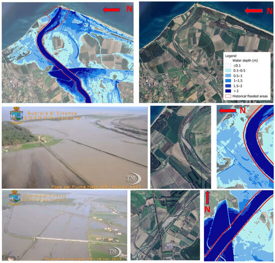
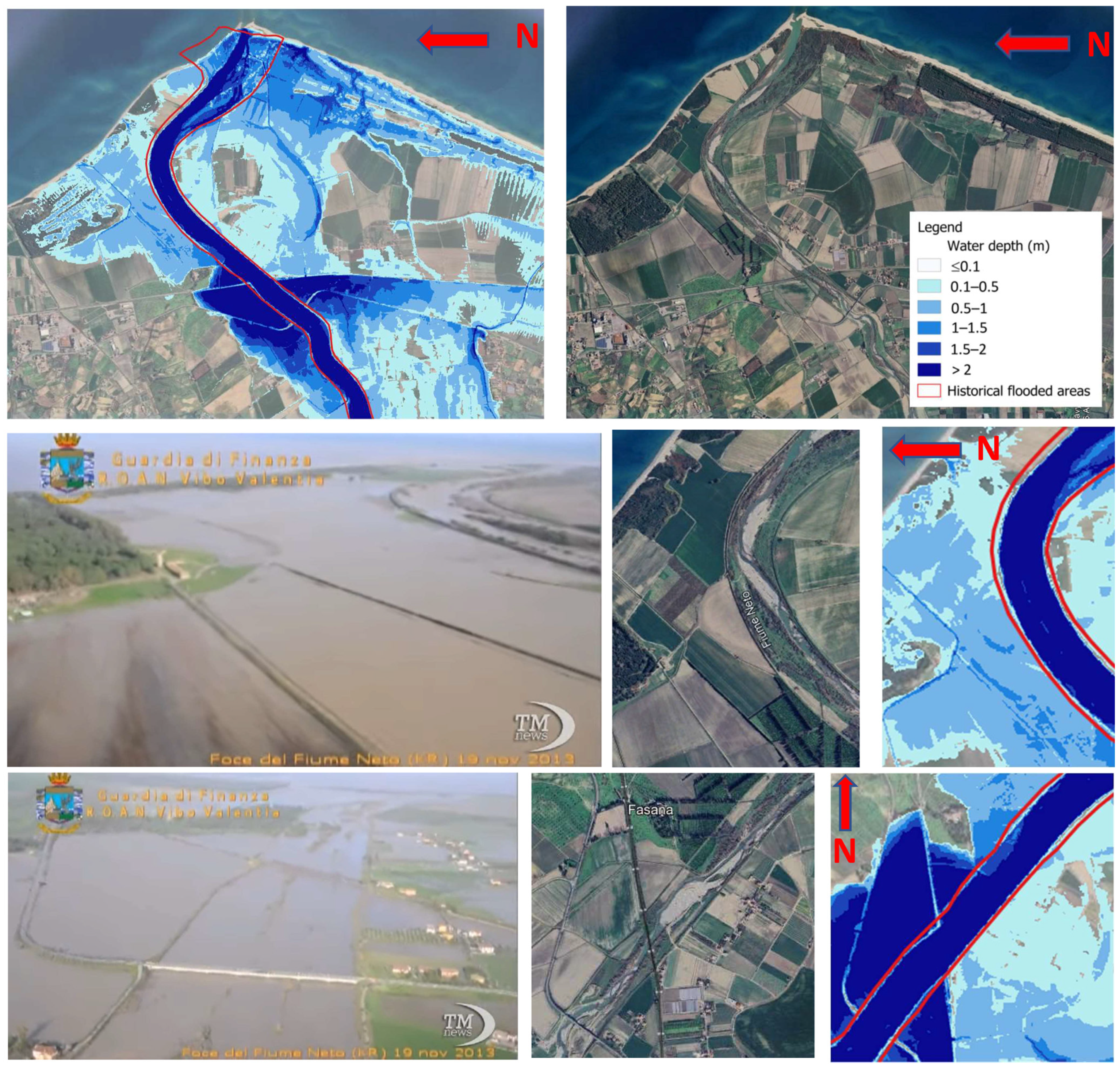
The valley area of the Neto River is actually subject to flooding in areas larger than those outlined by the red line in Figure 6. Indeed, Figure 7 shows flooding that was recorded on 19 November 2013. (AskaNews, https://youtu.be/AZC7Fe6-HII, accessed on 30 January 2026). As can be seen from Figure 7, even these areas are accurately identified by the results obtained with a 100-year return period. Here is an excerpt of the descriptive text (the original text is in Italian) associated with the video: “Crotone (askanews)—(…) A violent downpour caused the Neto River to overflow its banks in the area between Crotone and Strongoli. Aerial images from the Guardia di Finanza of Vibo Valentia document the situation in the countryside, where many homes were submerged by water, and residents were rescued by dinghies and helicopters. No casualties were reported, but several businesses reported damage, and the State Road 106 was partially closed to traffic, as were other provincial roads. In some cases, water reached two meters high, and some homes were submerged up to the first floor.” (https://youtu.be/AZC7Fe6-HII, accessed on 30 January 2026).
Figure 7.
Comparison between flooded areas and simulated ones for a 100-year return period. The images of the flooded areas are taken from the video reported in Askanews https://youtu.be/AZC7Fe6-HII, accessed on 30 January 2026.
As expected, the flooded area expands with increasing return periods. However, these increases remain relatively limited. Overall, compared to the flooded area with T = 50 years, the increase is approximately 6% for T= 100 years, 15% for T = 200 years, and 23% for T = 500 years.
Accurate calculation of spatially distributed hazard values is essential for risk analysis. Hazard level is expressed, for a given time t, as the product of water depth h (m) and flow velocity V (m/s). For the historical flooded areas, the calculated maxima hV values yielded the following average: hV = 1.491 m2/s for T = 50 years; hV = 1.687 m2/s for T = 100 years; hV = 1.877 m2/s for T = 200 years; hV = 2.156 m2/s for T = 500 years. These values were calculated within the present study based on the hydrodynamic simulations performed for the different return periods.
The results, in terms of increases, are summarized in Table 4.
Table 4.
Flooded area and average hazard increase ratios, with increasing return period from 50 to 500 years.
The results in Table 3 and Table 4 provide an empirical basis for analyzing the impact of hydrological uncertainty on hydraulic calculations. Notably, increasing the return period from 50 to 200 years (300%) results in only a 15% increase in flooded area, while hazard levels rise by 26%. For an increase from 50 to 500 years (900%), the flooded area grows by just 23%, while the hazard level rises by an average of 45%.
This conclusion is particularly significant when applied to the uncertainty associated with climate change. In other words, even substantial errors in estimating return period would not fundamentally alter the mapping of flash floods hazard areas in mountainous regions similar to Calabria. This demonstrates that the unpredictability of future flash flood-prone areas cannot be used as an excuse, as they can be identified with high reliability, even using relatively low return period events.
To put it another way, high return period events do not substantially alter the flooded area boundaries identified with lower return periods. Moreover, within these boundaries, even a significant increase in the return period results in only moderate changes in hydrodynamic variables.
This suggests that the proposed methodology enables reliable mapping of flash flood and rainfall-induced flood risks, even with currently available rainfall data.
The rain-on-grid hydrodynamic approach is a powerful tool; however, its application requires several key prerequisites. First, the availability of up-to-date, high-resolution topographic data is essential. In addition, the availability of statistically robust rainfall data at the regional scale and reliable land-use data are required. The approach also requires access to a reliable computational code based on the full shallow water equations (SWEs), as well as hardware capable of handling simulations over large spatial domains.
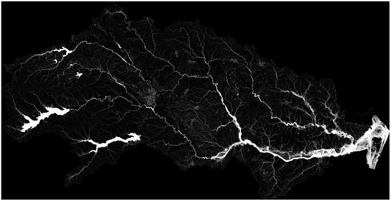
Despite these requirements, as demonstrated in this study, a significant advantage is that a single simulation, driven by an appropriately defined rainfall input, enables flood assessment over the entire territory. Figure 8 highlights the exceptionally high level of detail achieved by this procedure, demonstrating that the numerical simulation of all possible stormwater paths delivers a thorough and comprehensive assessment of the entire territory. This results in substantial savings in both time and cost compared to traditional methods, which are typically based on the aggregation of localized studies conducted in selected areas.
Figure 8.
The level of detail achieved by the simulation results, using a structured grid with 5 m × 5 m computational cells.
The methodology presented in this article was the basis for the update of the Flood Risk Management Plan for the Calabria Region, drawn up by the Southern Apennine District Basin Authority [40]. It can be usefully considered for studying flash floods that affect areas of Europe morphologically similar to Calabria.
5. Conclusions
In the preamble of Directive 2007/60/EC of the European Parliament and of the Council of 23 October 2007 on the assessment and management of flood risks, we read the following: “Member States should base their assessments, maps and plans on appropriate ‘best practice’ and ‘best available technologies’ not entailing excessive costs in the field of flood risk management.” Given the widespread anthropization of the territory, the population may be exposed to flood risk not only from large river overflows but also from much more localized events. Over the past 150 years, 56% of flood events in Europe have been classified as flash floods. In such a context, the challenge faced by those tasked with identifying and quantifying flood risk is the following: how to conduct analyses that can simultaneously assess both major river floods and all possible flood events that may occur at any point across the territory, from large river overflows to floods in small watercourses, and even localized flooding due to direct rainfall? The multiplication of potential flood or inundation points makes it extremely difficult to estimate risk through individual, localized studies, such as by analyzing each segment of the hydrographic network one by one. This would require conducting an enormous number of site-specific studies. But even if this were technically feasible, such an approach is not without its rigidity and limitations. In fact, the traditional approach, currently in widespread use, focuses on analyzing individual river sections. It is based on a method that presupposes an a priori selection of the watercourse segments on which to perform hydraulic analysis. This method requires inputting hydrographs of flow rates at both the upstream boundary of the studied section and at points where any tributaries enter along that section. As a contribution to overcoming these limitations, this work presented the authors’ experience in applying a complete hydrodynamic analysis over the entire river basin, considered as a single computational domain, where rainfall is used as a forcing input acting directly on each computational cell (the so-called rain-on-grid approach). In this way, the model can simultaneously simulate both surface runoff across slopes and the water that collects in depressions and talwegs defined by the topography. This approach does not require reliance on any predefined hydrographic network, as the result of the computation, fully consistent with the topography, will automatically identify the routed flow paths, thus defining the structure of the hydrographic network, from the main channels to the smallest upstream gullies, as well as all flood-prone areas due to rainwater ponding.
In this study it has been shown both theoretically and numerically that, using the Chicago hyetograph, it is possible to obtain with a single numerical simulation what would be obtained by performing a dedicated hydraulic calculation for each section of the considered basin, i.e., considering the individual critical event for each sub-basin and assuming a constant rainfall intensity corresponding to the rainfall of duration equal to the basin’s concentration time. In other words, this approach enables the determination of the critical peak flow rate, ensuring the constancy of the return period at any cross-section within the hydrographic network using a single simulation.
Procedures for handling the numerous minor crossings (such as small bridges, culverts, and road and railway underpasses) and for modeling dam outlets were also shown, all without the need to refine the computational grid or suspend the use of Shallow Water Equations (SWE).
This paper has shown the application of this methodology with reference to a sample area of about 1000 km2, coinciding with the Neto River Basin (Calabria, Italy). The analysis of the results showed that, even with the currently available hydrological data for Calabria, it is possible to achieve reliable flood mapping. This is thanks in part to the mountainous morphology of the region, which causes the extent of flooded areas to change only modestly, even under large variations in return periods.
This study demonstrated that a fully hydrodynamic rain-on-grid model was highly effective for producing flood hazard maps. Its ability to simulate surface runoff and localized flooding without a predefined hydrographic network was validated by strong agreement with observed flood events, confirming the method’s predictive reliability. Finally, the approach enabled high-resolution, comprehensive analysis across entire territories.
Author Contributions
Conceptualization, F.M.; methodology, F.M.; investigation, F.M.; data curation, F.M.; writing—original draft preparation, F.M.; writing—review and editing, A.A.G. and F.M.; visualization, A.A.G. and D.N.; supervision, F.M. All authors have read and agreed to the published version of the manuscript.
Funding
This research received no external funding.
Data Availability Statement
The original contributions presented in this study are included in the article. Further inquiries can be directed to the corresponding author.
Conflicts of Interest
The authors declare no conflicts of interest.
Appendix A
Actually, the area–time curve is not linear in real basins. Therefore, in this Appendix, an analysis is presented on some basins in Calabria to verify the degree of agreement between the peak flow calculated with the descending Chicago hyetograph and the one calculated using the rational formula.
Comparison with the rational formula
To verify that the CASp hyetograph, applied as rainfall input for the entire basin in the hydrodynamic model, leads to the critical flow in each section of the basin, several numerical tests were carried out for 42 sections of watercourses in Calabria, pertaining to four different basins (Ancinale, Corace, Ferro, and Savuto) (see Figure A1).
For the hydraulic simulations performed with the hydrodynamic model, the CASp hyetograph was discretized on an hourly basis.
For each sub-basin, the peak flows obtained from a single simulation over the entire basin were compared with those obtained individually from the application of the Rational Formula (QRF) for a certain number of sections along the hydrographic network branches.
The application of the rational formula requires, for each sub-basin, the estimation of the values of the coefficient φ and of the critical time of concentration, tc, which is the concentration time corresponding to the critical event for a given section and, therefore, to the critical intensity ().
For the estimation of the coefficient φ, the net rainfall calculation was carried out using the curve number (CN) method of the soil conservation service (SCS), considering an initial abstraction, prior to the onset of runoff.
The application of the curve number method provides the cumulative net rainfall depth for a fixed rainfall event duration, td. Consequently, the shape of the adopted design hyetograph does not change the total rainfall volume at time td. In other words, the net rainfall volume is invariant with respect to the shape of the design hyetograph. Therefore, the runoff volume calculated using the rational formula, equal to φitcAtc, is identical to the volume calculated with the descending hyetograph.
For a given excess rainfall depth and a specified rainfall duration, the distribution of rainfall intensity within this interval does not affect the total amount. Still, the maximum value of the excess rainfall depth over that time interval varies significantly depending on the temporal distribution of the entire hyetograph. This may differ depending on whether a Chicago hyetograph with the peak at the beginning (CASp), at the end, or in an intermediate position is considered.
These differences become smaller as soil moisture conditions increase and are nullified for fully saturated or completely impermeable soils.
In this study, the decreasing Chicago hyetograph was employed, as it has been proven to be the most suitable for the hydrological characteristics of the Calabria region [54,55]. On the other hand, the high CN values suggested by the guidelines minimize the differences that can be obtained with the different configurations of the Chicago hyetograph.
As for the estimation of tc, despite the numerous studies and formulas available in the literature (see, e.g., [56]), its determination is subject to much uncertainty.
In the present study, the concentration time tc for the 42 investigated sections was calculated as the time required for the entire basin to contribute to the surface runoff. It is generally expected that, all else being equal, the time of concentration is a function of rainfall intensity, decreasing as the intensity increases. To this end, through the application of the hydrodynamic model at the basin scale, a series of simulations with constant net intensity, iavg, was performed. In particular, values of iavg ranging from 2.5 to 100 mm/hour were tested.
For each hydrograph and, therefore, for each of the sub-basins corresponding to the 42 sections, the value of tc was derived as the temporal coordinate corresponding to 98% of the peak flow, having identified the latter as a sufficient value to consider the entire sub-basin contributing to the runoff. The values of tc show a decreasing trend as the constant average intensity that triggered the event increases. The relationship between tc and iavg follows a power law of the following form:
where A and B can be derived by imposing the best fit of the curve to the calculated values.
For a given area, the average intensity iavg is the one included in Equation (11), which is rewritten here as follows:
From Equations (A1) and (A2), the concentration time of the critical event (i.e., tc) was derived as the only unknown of the problem for each of the 42 sections. It does not vary much for the return periods analyzed here; therefore, a single value has been assumed for all return periods (see Table A1, Table A2, Table A3 and Table A4).
Once the value of tc was calculated for each sub-basin and for T = 50, 200, and 500 years, the calculation of QRF was performed using Equation (11). The results obtained in terms of QRF were compared, for each sub-basin and each value of T, with the peak flows obtained from the numerical simulations with the CASp hyetograph as input (see Table A5, Table A6, Table A7 and Table A8).
When considering data from the various Calabrian basins as a single dataset, the percentage error calculated as (QCASp − QRF)/QRF does not significantly change with increasing drainage area (see Figure A2). The peak flow values from the hydrodynamic model are systematically lower than those calculated with the rational method. On average, the difference remains extraordinarily constant with varying sub-basin areas. The average discrepancy is modest, around −7%. The maximum positive error is 9.5%, and the maximum negative error is −19.7%, while the root mean square error is 0.057.
These differences are because the rational method cannot account for the shape of the hyetograph and its convolution with the contributing areas of the basin, nor can it account for all the physical and geometric aspects that are considered in the hydrodynamic model.
Therefore, the descending hyetograph proved to be capable of providing a peak flow very close to that calculated with rainfall having the average intensity consistent with the IDF curve and the concentration time in any section of the hydrographic basin.
Thus, using the Chicago hyetograph, it is possible to obtain with a single numerical simulation what would be obtained by performing a dedicated hydraulic calculation for each section of the considered basin, i.e., considering the individual critical event for each sub-basin and assuming a constant rainfall intensity corresponding to the rainfall of duration equal to the basin’s concentration time. In conclusion, this approach enables the determination of the critical peak flow rate, ensuring the constancy of the return period at any cross-section within the hydrographic network using a single simulation.
Figure A1.
(a) Geographic location of the analyzed basins within the Calabria Region; (b) Geographic location of Calabria in Europe; (c) Savuto River basin; (d) Ancinale River basin; (e) Ferro River basin; (f) Corace River basin.
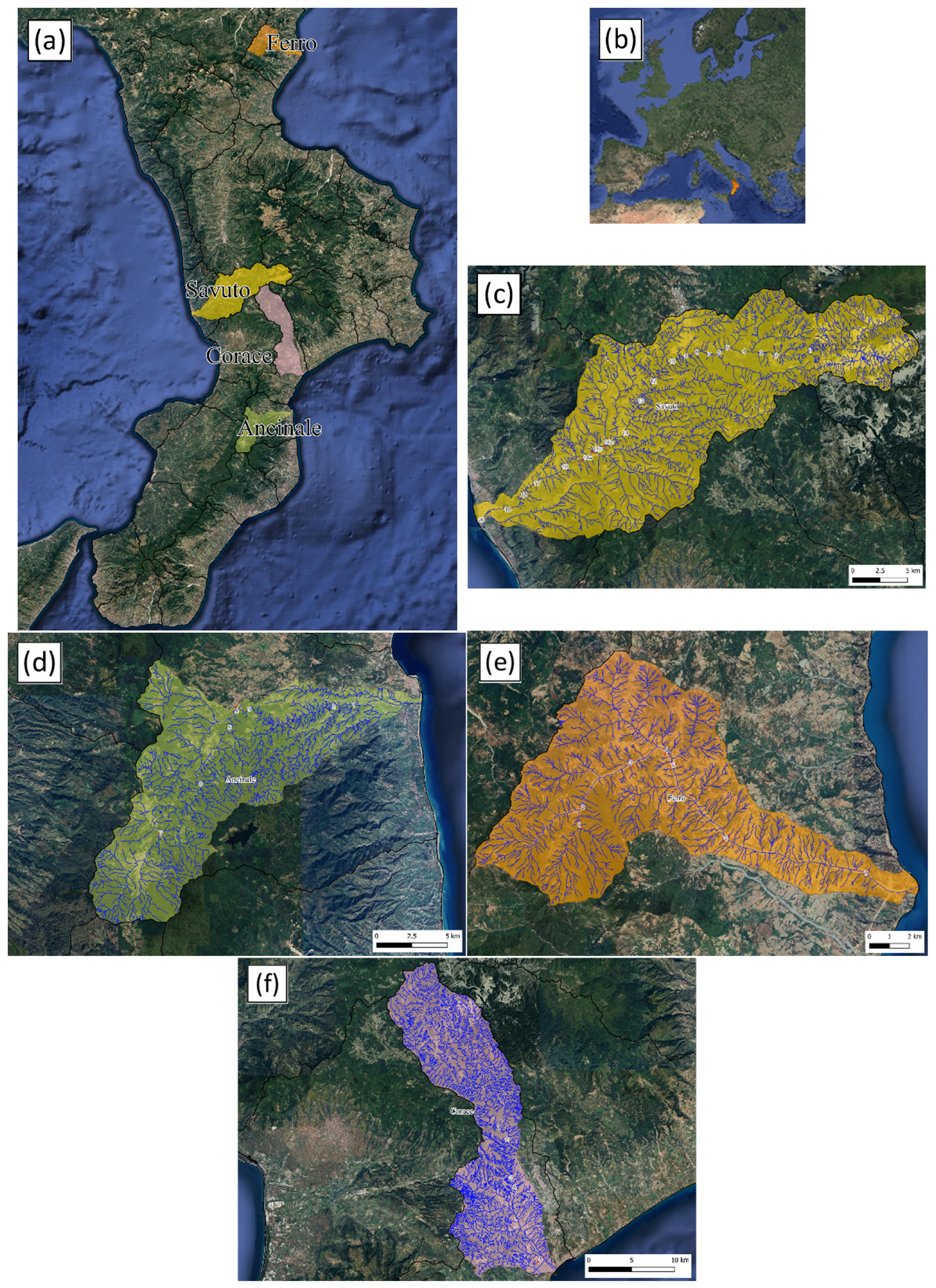
In the figures, the numbers indicate the sections for which the comparison was carried out between the discharge values provided by the rational formula and those obtained from the hydrodynamic model using the CASp hyetograph as rainfall input.
Figure A2.
Trend of the percentage error (QCASp − QRF)/QRF as a function of the basin area A.
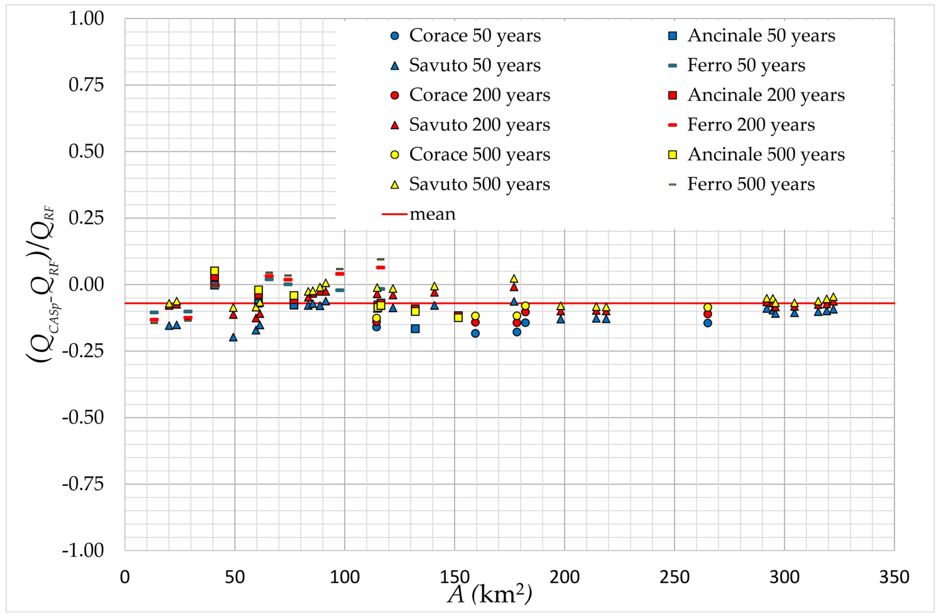
Table A1.
Time of concentration for the sub-basins considered in the Ancinale basin.
Table A2.
Time of concentration for the sub-basins considered in the Corace basin.
Table A3.
Time of concentration for the sub-basins considered in the Ferro basin.
Table A4.
Time of concentration for the sub-basins considered in the Savuto basin.
Table A5.
Comparison between QRF and QCASp for the Ancinale basin.
Table A6.
Comparison between QRF and QCASp for the Corace basin.
Table A7.
Comparison between QRF and QCASp for the Ferro basin.
Table A8.
Comparison between QRF and QCASp for the Savuto basin.
References
- European Environment Agency (EEA). Mapping the Impacts of Recent Natural Disasters and Technological Accidents in Europe: An Overwiev of the Last Decade; EEA Technical Report—No. 13; EEA: Copenhagen, Denmark, 2010. [Google Scholar]
- Douvinet, J.; Van De Wiel, M.J.; Delahaye, D.; Cossart, E. A flash flood hazard assessment in dry valleys (northern France) by cellular automata modelling. Nat. Hazards 2015, 75, 2905–2929. [Google Scholar] [CrossRef] [Scilit]
- Paprotny, D.; Sebastian, A.; Morales-Nápoles, O.; Jonkman, S.N. Trends in flood losses in Europe over the past 150 years. Nat. Commun. 2018, 9, 1985. [Google Scholar] [CrossRef] [Scilit]
- Ritter, J.; Berenguer, M.; Park, S.; Sempere-Torres, D. Real-time assessment of flash flood impacts at pan-European scale: The ReAFFINE method. J. Hydrol. 2021, 603, 127022. [Google Scholar] [CrossRef] [Scilit]
- Gaume, E.; Bain, V.; Bernardara, P.; Newinger, O.; Barbuc, M.; Bateman, A.; Blaškovičová, L.; Blöschl, G.; Borga, M.; Dumitrescu, A.; et al. A compilation of data on European flash floods. J. Hydrol. 2009, 367, 70–78. [Google Scholar] [CrossRef] [Scilit]
- HANZE: Historical Analysis of Natural Hazards in Europe; Faculty of Civil Engineering and Geosciences, Department of Hydraulic Engineering, T. U. Delft: Delft, The Netherlands, 2017. [CrossRef]
- Yang, B.; Yuan, X.; Tang, F.; Liu, D. Small wetlands: Critical to flood management. Science 2024, 386, 6724. [Google Scholar] [CrossRef] [Scilit]
- Llasat, M.C. Spain’s flash floods reveal a desperate need for improved mitigation efforts. Nature 2024, 635, 787. [Google Scholar] [CrossRef] [Scilit] [PubMed]
- European Environment Agency (EEA). Responding to Climate Change Impacts on Human Health in Europe: Focus on Floods, Droughts and Water Quality; EEA Report—No. 3; EEA: Copenhagen, Denmark, 2024. [Google Scholar]
- Castro, D.R.; Shahi, K.R.; Sairam, N.; Fischer, M.; Mohor, G.S.; Thieken, A.; Dewals, B.; Kreibich, H. Key drivers of flash flood damage to private households. J. Flood Risk Manag. 2025, 18, e70088. [Google Scholar] [CrossRef] [Scilit]
- Cornwall, W. Europe’s deadly floods leave scientists stunned. Science 2021, 373, 6553. [Google Scholar] [CrossRef] [Scilit] [PubMed]
- Blöschl, G.; Hall, J.; Parajka, J.; Perdigão, R.A.P.; Merz, B.; Arheimer, B.; Aronica, G.T.; Bilibashi, A.; Bonacci, O.; Borga, M.; et al. Changing climate shifts timing of European floods. Science 2017, 357, 6351. [Google Scholar] [CrossRef] [Scilit] [PubMed]
- Alfieri, L.; Salamon, P.; Bianchi, A.; Neal, J.; Bates, P.; Feyen, L. Advances in pan-European flood hazard mapping. Hydrol. Process 2014, 28, 4067–4077. [Google Scholar] [CrossRef] [Scilit]
- Dottori, F.; Salamon, P.; Bianchi, A.; Alfieri, L.; Hirpa, F.A.; Feyen, L. Development and evaluation of a framework for global flood hazard mapping. Adv. Water Resour. 2016, 94, 87–102. [Google Scholar] [CrossRef] [Scilit]
- Sampson, C.C.; Smith, A.M.; Bates, P.D.; Neal, J.C.; Alfieri, L.; Freer, J.E. A high-resolution global flood hazard model. Water Resour. Res. 2015, 51, 7358–7381. [Google Scholar] [CrossRef] [Scilit]
- Wing, O.E.J.; Bates, P.D.; Sampson, C.C.; Smith, A.M.; Johnson, K.A.; Erickson, T.A. Validation of a 30 m resolution flood hazard model of the conterminous United States. Water Resour. Res. 2017, 53, 7968–7986. [Google Scholar] [CrossRef] [Scilit]
- Wing, O.E.J.; Bates, P.D.; Quinn, N.D.; Savage, J.T.S.; Uhe, P.F.; Cooper, A.; Collings, T.P.; Addor, N.; Lord, N.S.; Hatchard, S.; et al. A 30 m Global Flood Inundation Model for Any Climate Scenario. Water Resour. Res. 2024, 60, e2023WR036460. [Google Scholar] [CrossRef] [Scilit]
- Peker, I.B.; Gülbaz, S.; Demir, V.; Orhan, O.; Beden, N. Integration of HEC-RAS and HEC-HMS with GIS in Flood Modeling and Flood Hazard Mapping. Sustainability 2024, 16, 1226. [Google Scholar] [CrossRef] [Scilit]
- Nguyen, P.; Thorstensen, A.; Sorooshian, S.; Hsu, K.; AghaKouchak, A.; Sanders, B.; Koren, V.; Cui, Z.; Smith, M. A high resolution coupled hydrologic- hydraulic model (HiResFlood-UCI) for flash flood modeling. J. Hydrol. 2016, 541, 401–420. [Google Scholar] [CrossRef] [Scilit]
- Yamazaki, D.; Kanae, S.; Kim, H.; Oki, T. A physically based description of floodplain inundation dynamics in a global river routing model. Water Resour. Res. 2011, 47, W04501. [Google Scholar] [CrossRef] [Scilit]
- Rajib, A.; Liu, Z.; Merwade, V.; Tavakoly, A.A.; Follum, M.L. Towards a large-scale locally relevant flood inundation modeling framework using SWAT and LISFLOOD-FP. J. Hydrol. 2020, 581, 124406. [Google Scholar] [CrossRef] [Scilit]
- Huang, S.; Hattermann, F.F. Coupling a global hydrodynamic algorithm and a regional hydrological model for large-scale flood inundation simulations. Hydrol. Res. 2018, 49, 438–449. [Google Scholar] [CrossRef] [Scilit]
- Costabile, P.; Costanzo, C.; Macchione, F. Comparative analysis of overland flow models using finite volume schemes. J. Hydroinform. 2012, 14, 122–135. [Google Scholar] [CrossRef] [Scilit]
- Kim, J.; Warnock, A.; Ivanov, V.Y.; Katopodes, N.D. Coupled modeling of hydrologic and hydrodynamic processes including overland and channel flow. Adv. Water Resour. 2012, 37, 104–126. [Google Scholar] [CrossRef] [Scilit]
- Xia, X.; Liang, Q.; Ming, X. A full-scale fluvial flood modelling framework based on a high-performance integrated hydrodynamic modelling system (HiPIMS). Adv. Water Resour. 2019, 132, 103392. [Google Scholar] [CrossRef] [Scilit]
- Ennouini, W.; Fenocchi, A.; Petaccia, G.; Persi, E.; Sibilla, S. A complete methodology to assess hydraulic risk in small ungauged catchments based on HEC-RAS 2D Rain-On-Grid simulations. Nat. Hazards 2024, 120, 7381–7409. [Google Scholar] [CrossRef] [Scilit]
- Bates, P.D.; Horritt, M.S.; Fewtrell, T.J. A simple inertial formulation of the shallow water equations for efficient two-dimensional flood inundation modelling. J. Hydrol. 2010, 387, 33–45. [Google Scholar] [CrossRef] [Scilit]
- Sharifian, M.K.; Kesserwani, G.; Chowdhury, A.A.; Neal, J.; Bates, P. LISFLOOD-FP 8.1: New GPU-accelerated solvers for faster fluvial/pluvial flood simulations. Geosci. Model Dev. 2023, 16, 2391–2413. [Google Scholar] [CrossRef] [Scilit]
- Shaw, J.; Kesserwani, G.; Neal, J.; Bates, P.; Sharifian, M.K. LISFLOOD-FP 8.0: The new discontinuous Galerkin shallow-water solver for multi-core CPUs and GPUs. Geosci. Model Dev. 2021, 14, 3577–3602. [Google Scholar] [CrossRef] [Scilit]
- Costabile, P.; Costanzo, C.; Macchione, F. A storm event watershed model for surface runoff based on 2D fully dynamic wave equations. Hydrol. Process. 2012, 27, 554–569. [Google Scholar] [CrossRef] [Scilit]
- Macchione, F.; Lombardo, M. Roughness-based method for simulating hydraulic consequences of both woody debris clogging and breakage at bridges in basin-scale flood modeling. Water Resour. Res. 2021, 57, e2021WR030485. [Google Scholar] [CrossRef] [Scilit]
- Varra, G.; İnan, Ç.A.; Della Morte, R.; Tartaglia, M.; Fiduccia, A.; Zammuto, A.; Agostino, I.; Cozzolino, L. Assessment of direct rainfall and flood-induced damage to land transport infrastructure using two-dimensional HEC-RAS 6.6 rain-on-grid simulations. Nat. Hazards 2025, 121, 17615–17645. [Google Scholar] [CrossRef] [Scilit]
- Morales-Hernández, M.; Sharif, B.; Kalyanapu, A.; Ghafoor, S.; Dullo, T.; Gangrade, S.; Kao, S.-C.; Norman, M.; Evans, K. TRITON: A Multi-GPU Open Source 2D Hydrodynamic Flood Model. Environ. Model. Softw. 2021, 141, 105034. [Google Scholar] [CrossRef] [Scilit]
- Ma, R.; Han, H.; Zhang, Z. An Integrated Hydrological–Hydrodynamic Model Based on GPU Acceleration for Catchment Scale Rainfall Flood Simulation. Atmosphere 2025, 16, 809. [Google Scholar] [CrossRef] [Scilit]
- Blöschl, G.; Buttinger-Kreuzhuber, A.; Cornel, D.; Eisl, J.; Hofer, M.; Hollaus, M.; Horváth, Z.; Komma, J.; Konev, A.; Parajka, J.; et al. Hyper-resolution flood hazard mapping at the national scale. Nat. Hazards Earth Syst. Sci. 2023, 24, 2071–2091. [Google Scholar] [CrossRef] [Scilit]
- Iovine, G.G.R.; Greco, R.; Gariano, S.L.; Pellegrino, A.D.; Terranova, O.G. Shallow-landslide susceptibility in the Costa Viola mountain ridge (southern Calabria, Italy) with considerations on the role of causal factors. Nat. Hazards 2014, 73, 111–136. [Google Scholar] [CrossRef] [Scilit]
- Tufano, R.; Guerriero, L.; Corona, M.A.; Cianflone, G.; Di Martire, D.; Ietto, F.; Novellino, A.; Rispoli, C.; Zito, C.; Calcaterra, D. Multiscenario flood hazard assessment using probabilistic runoff hydrograph estimation and 2D hydrodynamic modelling. Nat. Hazards 2023, 116, 1029–1051. [Google Scholar] [CrossRef] [Scilit]
- Zhang, W.; Cundy, T.W. Modeling of two-dimensional overland flow. Water Resour. Res. 1989, 25, 2019–2035. [Google Scholar] [CrossRef] [Scilit]
- Artiglieri, P.; Curulli, G.; Coscarella, F.; Ferraro, D.A.; Macchione, F. Performance of HEC-RAS v6.5 at basin scale for calculating the flow hydrograph: Comparison with TUFLOW. Nat. Hazards 2025, 121, 9477–9490. [Google Scholar] [CrossRef] [Scilit]
- Macchione, F.; Algieri Ferraro, D.; Curulli, G.; Ruffolo, A. Treatment of culverts and road underpasses for large-scale flood modelling. In Technologies for Integrated River Basin Management; Frega, C.G., Macchione, F., Eds.; Proceedings 44th Italian Conference on Integrated River Basin Management; EdiBios: Cosenza, Italy, 2023; Volume 44, pp. 165–174. [Google Scholar]
- Macchione, F.; Algieri Ferraro, D.; Curulli, G.; Bonelli, R.; Giuzio, L.; Velardo, R.; Corbelli, V. Innovative criteria for large-scale hydraulic risk analysis aimed at update of both PAI and PGRA maps. In Technologies for Integrated River Basin Management; Frega, C.G., Macchione, F., Eds.; Proceedings 45th Italian Conference on Integrated River Basin Management; EdiBios: Cosenza, Italy, 2024; Volume 44, pp. 19–28. [Google Scholar]
- Keifer, C.J.; Chu, H.H. Synthetic storm pattern for drainage design. J. Hydraul. Div. 1957, 83, 1–25. [Google Scholar] [CrossRef] [Scilit]
- Beven, K.J. Rainfall-Runoff Modelling: The Primer; John Wiley & Sons: Hoboken, NJ, USA, 2012. [Google Scholar]
- Pilgrim, D.H.; Cordery, I. Flood runoff. In Handbook of Hydrology; Maidment, D.R., Ed.; McGraw-Hill: New York, NY, USA, 1992. [Google Scholar]
- Lapides, D.A.; Sytsma, A.; Thompson, S. Implications of distinct methodological interpretations and runoff coefficient usage for rational method predictions. J. Am. Water Resour. Assoc. 2021, 57, 859–874. [Google Scholar] [CrossRef] [Scilit]
- Viparelli, C. Ricostruzione dell’Idrogramma di Piena; Stab. Tip. Genovese, Napoli, No. 12; Istituto di Idraulica dell’Università di Palermo: Palermo, Italy, 1961. [Google Scholar]
- Merz, R.; Blöschl, G.; Parajka, J. Spatio-temporal variability of event runoff coefficients. J. Hydrol. 2006, 331, 591–604. [Google Scholar] [CrossRef] [Scilit]
- Penta, A. Caratteristiche pluviometriche e climatiche della Calabria. In Tecniche per la Difesa dall’Inquinamento; EdiBios: Cosenza, Italy, 2011; pp. 475–492. [Google Scholar]
- Ferrari, E. Peculiarità fisiche e rischio idraulico delle fiumare calabre. In Tecniche per la Difesa dall’Inquinamento; EdiBios: Cosenza, Italy, 2012; pp. 107–123. [Google Scholar]
- Macchione, F.; Lombardo, M.; Ruffolo, A.; Algieri Ferraro, D. Shallow water equations applied to the basin scale for flood risk analysis. In Scaling and Extremes in Water Science; De Bartolo, S., Francone, A., Saponieri, A., Tomasicchio, G.R., Eds.; Milella: Lecce, Italy, 2023. [Google Scholar]
- Biondi, D.; Cruscomagno, F.; De Luca, D.L.; Ferrari, E.; Versace, P. La Valutazione delle Piene in Calabria: 1989–2013. In Atti del XXXIV Corso di Aggiornamento Tecniche per la Difesa dall’Inquinamento; EdiBios: Cosenza, Italy, 2013; Volume 34, pp. 187–216. [Google Scholar]
- U.S. Soil Conservation Service. National Engineering Handbook, Section 4: Hydrology; U.S. Department of Agriculture: Washington, DC, USA, 1972.
- Gharakhanlou, N.M.; Perez, L. Flood susceptible prediction through the use of geospatial variables and machine learning methods. J. Hydrol. 2023, 617, 129121. [Google Scholar] [CrossRef] [Scilit]
- Terranova, O.G.; Iaquinta, P. Temporal properties of rainfall events in Calabria (southern Italy). Nat. Hazards Earth Syst. Sci. 2011, 11, 751–757. [Google Scholar] [CrossRef] [Scilit]
- Terranova, O.G.; Gariano, S.L. Rainstorms able to induce flash floods in a Mediterranean-climate region (Calabria, southern Italy). Nat. Hazards Earth Syst. Sci. 2014, 14, 2423–2434. [Google Scholar] [CrossRef] [Scilit]
- Grimaldi, S.; Petroselli, A.; Tauro, F.; Porfiri, M. Time of concentration: A paradox in modern hydrology. Hydrol. Sci. J. 2012, 57, 217–228. [Google Scholar] [CrossRef] [Scilit]

Disclaimer/Publisher’s Note: The statements, opinions and data contained in all publications are solely those of the individual author(s) and contributor(s) and not of MDPI and/or the editor(s). MDPI and/or the editor(s) disclaim responsibility for any injury to people or property resulting from any ideas, methods, instructions or products referred to in the content. |
© 2026 by the authors. Licensee MDPI, Basel, Switzerland. This article is an open access article distributed under the terms and conditions of the Creative Commons Attribution (CC BY) license.