


Abstract
Groundwater resources are critical in sustaining rapidly growing coastal urban regions like Dili City, Timor-Leste, where aquifers are prone to contamination. To inform groundwater pollution prevention and control in the Quaternary intergranular aquifer, a GIS-based groundwater vulnerability assessment was carried out using DRASTIC, modified DRASTIC, and modified DRASTIC–AHP methodologies. It confirmed that the central to northern urban area was the most vulnerable, while the southern part was the least vulnerable to contamination. Model performance was validated by correlating vulnerability indices with measured groundwater quality parameters, showing that the modified DRASTIC–AHP was the most accurate. The areas classified as having very low, low, moderate, high and very high vulnerability were 23.1%, 23.1%, 20.6%, 12.8%, and 19.2%, respectively, with high vulnerability along the northern coastline and Comoro River alluvial channel. Sensitivity analysis supports model robustness and identifies recharge, aquifer media, and hydraulic conductivity as the dominant controlling factors. The integrated modeling and sensitivity framework provides an efficient basis for prioritizing protection measures and infrastructure upgrades (e.g., sewerage) to reduce contamination risks. A key management implication is that centralized wastewater management is preferable to current practices for mitigating ongoing groundwater degradation.
1. Introduction
Globally, groundwater is a preferred choice for drinking water in many regions because of its quality, availability, and accessibility [1,2]. Nonetheless, many unanswered concerns remain, including how well-known groundwater contaminants behave and the influence of different land uses on groundwater quality. Human activities like groundwater use, land-use changes, and pollution, combined with the natural complexity of the water cycle, make aquifers in populated areas vulnerable [3]. Therefore, knowledge of the vulnerability of aquifers is essential for efficient and effective groundwater management, to ensure the safe and sustainable use of this resource [4,5].
Dili City sits above an aquifer composed of Quaternary sediment deposited on Permian metamorphic rocks, and this has acted as the most important source for water supply over the past two decades [6]. Precipitation is the main source of groundwater, recharging via surface watersheds in the Dili Basin from south to northward (S-N) [6,7,8]. This water resource caters directly to the local community through private on-site wells and indirectly via production wells under the jurisdiction of the Timor-Leste National Company, specifically BEE Timor-Leste E.P. Dili City has undergone substantial urbanization and infrastructural development, evolving into a center for governmental, economic, healthcare, and educational activities [9]. Consequently, the escalating demand for groundwater, coupled with increasing domestic wastewater production (largely unmanaged), has emerged as a significant concern. The aquifer system is formed by a sequence of unconsolidated sediments that are permeable, largely unconfined, and thus highly susceptible to pollution.
Various boreholes and tubewells, deployed over recent years to meet both domestic and non-domestic needs, contribute to heightened groundwater usage. The rapid urbanization of Dili has also led to major alterations in landform. As the capital of the Republica de Democrática de Timor-Leste (RDTL), the city now has nearly 90% of its land covered by civil construction, including residential buildings, offices, and roads. Despite the majority of the local community relying on groundwater in Dili, there exists a limited understanding of groundwater’s vulnerability to pollution.
While previous studies have highlighted issues such as increased bacteria and nitrate levels in shallow groundwater in certain areas [10], a comprehensive delineation of the vulnerability of different areas to groundwater quality (or quantity) depletion remains lacking. The Analytic Hierarchy Process (AHP) has been employed to identify groundwater potential zones, but it did not specifically address groundwater pollution vulnerability [6]. Another recent study conducted in Dili City employed various approaches to evaluate issues associated with wastewater and potential options to mitigate effects on health and the environment [11], but, to date, there has been no mapping of the most vulnerable zones for groundwater pollution in Dili City.
A fundamental challenge in groundwater protection is rapid urbanization, changing consumer habits, and a lack of concern for the environment [12]. Limited attention has been paid to wastewater management and its possible interactions with underlying groundwater, such as the flow of commercial and residential wastewater (and pollutants) into groundwater or river networks through septic tanks. While some facilities, such as government offices, hotels, and hospitals, are responsible for their liquid waste management, wastewater management remains lacking for other sources, leading to the unregulated release of wastewater into water bodies and the environment. Up until the present, a significant portion of wastewater, including domestic and non-domestic wastewater flows, has been released directly onto the ground and/or via canals into the ocean at Dili’s northern Coastline [10,11]. Concerns about wastewater discharges and their impact on groundwater quality are a focus of this study because of the inherent risks to groundwater from increasing wastewater releases.
The absence of a thorough assessment of groundwater vulnerability to pollution in Dili city (and Timor-Leste more generally) stems largely from inadequate data availability and manpower. On the other hand, it is complex to remediate polluted groundwater due to its high cost and technical challenges [13,14]. Motivated by these conditions, there is a pressing need to enhance research into groundwater vulnerability to assist policymakers in creating effective groundwater quality management in Dili City.
Groundwater vulnerability assessment is a crucial process in determining the level of risk in certain areas to a specific threat, whether natural or man-made [15]. Such an approach offers a thorough and data-driven way to understand pollution risks to groundwater, and thereby facilitates better-informed, more sustainable groundwater and land-use management practices [16,17]. The idea behind vulnerability assessment is that aquifers are heterogeneous and some areas are more susceptible to deterioration in quality (or quantity) than others [18]. The process of vulnerability mapping is relatively time-efficient (provided data are available) and the output(s) are generally accessible and informative to policy makers and the public [19].
Several approaches are available, including index-overlay techniques, which identify groundwater locations that are prone to pollution by using weights, indexes, and range values [19]. The commonly used models for groundwater vulnerability are DRASTIC [20], SINTACS [21], GOD [22], AVI [23], and PI [24]. DRASTIC is the most widely used groundwater vulnerability model, due to its simplicity, low data requirements, and straightforward explanation of groundwater vulnerability [25]. However, a significant drawback of the model is that it does not take into account how groundwater systems change over time (e.g., shifts in land use), which can cause errors in assessing vulnerability, especially in areas that have changed significantly over time [26].
The DRASTIC model with GIS was first introduced by Merchant [27], while sensitivity analyses were first described by [28] as a way to check the robustness of the DRASTIC analyses. Many researchers worldwide have used the model to assess groundwater vulnerability in urban areas [16,29,30,31]. Studies by [32] compared DRASTIC to GOD and SINTACS to evaluate how effectively these models perform and found that DRASTIC was the most efficient, although sensitivity analyses were not performed to address potential biases in DRASTIC caused by the subjectivity of the weights assigned to different input factors. Other studies [29,30,33] used sensitivity analysis of groundwater vulnerability through map removal and single-parameter sensitivity analyses, aiming to enhance the robustness of DRASTIC and to identify the most influential parameter(s) in the model output. Additionally, Refs. [26,34,35,36] successfully conducted validated vulnerability modeling through ground-truthing and monitoring nitrate contamination, which is considered to be of anthropogenic origin.
Given the complexity of hydrogeological settings and the various anthropogenic activities that contribute to groundwater vulnerability over time, the inherent uncertainty and limited applicability of any single method may lead to inaccurate results when applied to a specific area [37]. In Dili City, several groundwater studies have been conducted over the past ten years [6,7,8,9,10,11], but groundwater vulnerability assessment remains unexplored. By incorporating an array of field data within a GIS framework, this study aimed to produce a vulnerability map for the Dili aquifer using DRASTIC, modified DRASTIC, and applying the Analytic Hierarchy Process (AHP) to minimize bias, as well as conducting a sensitivity analysis to identify the most influential factors in the vulnerability assessment. To confirm the model’s accuracy and practicality, we used nitrate and total coliform measurements in groundwater as an indicator of anthropogenic impact to validate the vulnerability maps, discussing their suitability for the specific context of Dili. A key insight and value of this study is highlighting the implications of the vulnerability mapping for wastewater management and public health. The findings are expected to assist decision-makers in effectively controlling the environmental impacts caused by the prevalent issue of inadequate wastewater management, together with unregulated drilling and groundwater extraction. Furthermore, the study intended to contribute to enhancing the local community’s awareness of the environmental consequences associated with groundwater exploitation and the lack of attention to sanitation infrastructure and practices.
The DRASTIC method has been widely used to assess groundwater vulnerability to pollution, and its application is certainly not novel internationally. The novelty of this paper lies in the use of total coliforms to validate the model results, which, for the specific context of Dili, offers advantages over the typically used nitrates, as is explained below, and can be applied elsewhere internationally where similar conditions exist. Importantly, in the context of Timor-Leste, this study represents the first attempt to model groundwater vulnerability to pollution in its capital, Dili, which has tremendous potential for unlocking future research work, advancing wastewater management, and promoting public health.
2. Materials and Methods
2.1. Description of the Study Area
The focus of this research was the alluvial aquifers of Dili City (an area of ~26 km2), where groundwater abstraction is important for water supply to residences, local businesses, and government buildings (Figure 1). The capital has a population of approximately 317,569 and covers the administrative posts of Cristo Rei, Dom Aleixo, Nain Feto, and Vera Cruz [38]. The dense population creates stress on groundwater quantity and quality, as the majority of residents consume groundwater through private wells. The climate is characterized by the northwest and southeast monsoons. From October to February, the climate is dominated by the northwest monsoon, which moves from the South China Sea and is accompanied by high humidity and heavy rainfall. Tropical cyclones can affect the study area from December to April. The dry air of the southeast monsoon, which blows from Australia to Timor-Leste from the south, has an impact on the climate from April to September, bringing high temperatures and a long, pronounced dry season [8,39]. The average annual rainfall in the study area is 994 to 1223 mm/year [6], and the average temperature is typically around 27 °C in coastal areas and around 22 °C in the highlands [7]. The available rainfall data indicate that 81% of the total rainfall occurs during the wet season (November to April).
Figure 1.
(a) Geological map of the study area in Dili City, Timor-Leste, and groundwater sampling points for Coliform analysis. (b) 2D subsurface lithology distribution across the area [8].
Geologically, Timor is located at the collisional margin between the Australian continental margin and the oceanic Banda volcanic arc [40]. The geology and hydrogeology of Dili have been documented in several reports and maps. The flat area of Dili City is composed of alluvial deposits, including sand, gravel, clay, and silt, while the southern mountainous area of Dili primarily consists of metamorphic rocks, such as slate, phyllite, schist, and metabasite [41,42]. A recent study by [8] described the subsurface lithology as consisting of gravelly sand, clay, and bedrock (Figure 1b). The study also reported that the clay layer is abundant in zone two of Dili; however, its distribution is uneven, leading to semi-confined aquifer conditions in places.
The Dili aquifer is recharged through lateral flow, which occurs via mountain block recharge processes, as well as by the infiltration of precipitation and surface water. It should be noted that the ephemeral Comoro River channel is highly permeable and carries significant runoff from the mountains south of Dili during the wet season [6,8].
Dili’s groundwater can be contaminated when unregulated land use and wastewater introduce pollutants, with the contamination process strongly mediated/controlled by the type of soil and aquifer characteristics. The Dili region is characterized by silty soils, sandy soils, and clay loams. Sandy soils and silty soils typically have medium to poor water-holding capacity and can easily transmit contaminants, while clay loams are excellent water-holders and can act as a barrier [43]. The unconsolidated sediments in the flat area of the city form an intergranular aquifer system, while the metamorphic rocks to the south form fractured-rock aquifers [7]. The region has unconfined, semi-confined, and confined aquifers with varying amounts/proportions of sand and gravel, and the spatial distribution of such remains a key gap in hydrogeology knowledge in the area. The soil thickness ranges from 1 to 3 m, while the unconfined aquifer thickness is generally 10–30 m [8]. Unconfined aquifers are naturally more susceptible to contamination than confined aquifers. The city is characterized by a lack of wastewater management, whereby open drains around residences directly connect household gray and black water, and commercial and industrial wastewater (Figure 1) [9,11]. Septic tanks that do not follow standard construction techniques are widespread across the city. Septic tanks can easily contaminate domestic wells tapping the shallow water table and contribute to the presence of bacteria such as Escherichia coli (E. coli) and coliform, especially in shallow groundwater around high-density residential areas [10].
Coliform bacteria are commonly understood to originate from point-source contamination processes. However, in the context of Dili, it is plausible to consider them to have originated from diffuse sources because of the widespread presence of domestic wastewater from the innumerable septic tanks, the vast network of open canals that transport wastewater and often flood during the wet season, and flooding from the streams and rivers that cross the Dili area (Figure 1). The study by [11] reveals that people dispose of 47.7% of domestic wastewater in open sewer canals, 24.6% in domestic gardens, and 27.7% in septic tanks. Domestic wastewater is typically discharged along sewer canals across the city and existing rivers due to the absence of a wastewater collection and treatment system. Wastewater can seep through the sewer canals, streams, and rivers, moving down through the loose sediments in the unsaturated zone, polluting shallow aquifers and causing widespread contamination, which is aggravated by the high density of the point sources.
2.2. Materials and Methods
The DRASTIC model and variations were employed to evaluate the susceptibility of the aquifer in Dili City to pollution, which was done in combination with groundwater sampling for contamination indicators. Nitrate and total coliform concentrations in groundwater were used to validate the model. The kriging method was applied to demonstrate the trend of DRASTIC variables. In contrast to other types of geographical interpolation, kriging uses a statistical model called a “variogram” to objectively estimate spatial weights, rather than relying on a random mathematical function; this model calculates the variance at each location, serving as an indicator of the reliability of the spatial interpolation [44].
Shape files were exported to ArcGIS—a Geographic Information System (GIS)—and displayed alongside the relevant data sets. An interactive geodatabase was set up, geographical data was compiled, vulnerability maps were created, DRASTIC indices were calculated, and sensitivity analysis was carried out using Arc GIS 10.3. As shown in Figure 2, the methodology for processing, validating, and presenting the final vulnerability maps was modified [45].
Figure 2.
Methodological framework of groundwater vulnerability assessment integrating DRASTIC, modified DRASTIC, and AHP approaches.
2.2.1. Development of DRASTIC Parameters
DRASTIC is an empirical groundwater model used to assess groundwater vulnerability within aquifer systems, relying on in situ hydrogeological information [20]. The method involves assessing and weighting seven main characteristics of the hydrogeological system that affect groundwater pollution risk: depth to the water table (D), net recharge (R), aquifer media (A), soil media (S), topography (T), impact of the vadose zone (I), and the hydraulic conductivity (C) of the aquifer [20]. To assess the relative vulnerability of groundwater to pollution, the model employs a numerical ranking approach that assigns different weights and ratings to these parameters. A higher DRASTIC index indicates a higher potential for contamination, and vice versa.
Zones that are more prone to contamination can be identified after the DRASTIC index has been calculated. The following presumptions form the basis of the methodology: (a) possible sources of contamination are found on the soil’s surface; (b) infiltration allows these sources to enter the aquifer; (c) the contaminant is as mobile as groundwater; and (d) the hydrogeological unit under consideration is larger than 40 hectares in surface area [20].
Weights range from 1 to 5, and the numerical relative ranking is between 1 and 10 [20]. The most significant and vulnerable parameter is assigned a weight of 5, whereas the least significant and least vulnerable parameter is given a weight of 1, as summarized in Table 1. The additive Equation (1) can be used to calculate the final vulnerability, which is a weighted total of the seven previously indicated parameters:
where D, R, A, S, T, I, and C are the seven parameters; r is the rating value of the analyzed area; and w is the weight associated with each parameter [30]. Every parameter in this model possesses a set amount of weight and rate, determined by its significance in the setting and its influence on the aquifer’s susceptibility [46]. This research incorporated land use and land cover (L) as a key feature in the modified DRASTIC model, alongside the original DRASTIC methodology. The formula for the enhanced DRASTIC index is delineated in the modified Equation (2):
Di = DrDw + RrRw + ArAw + SrSw + TrTw + IrIw + CrCw
Di = DrDw + RrRw + ArAw + SrSw + TrTw + IrIw + CrCw + Lrlw
Table 1.
The DRASTIC, modified DRASTIC, and modified DRASTIC–AHP models incorporate parameters along with their rating (R), weight (W), and index (I) values, modified from [20,26,36].
These weights and scores are determined using the Delphi technique, which is well defined and used worldwide [26,34,35,36]. Areas with higher index values are considered to be more vulnerable to contamination of groundwater. Table 2 provides a summary of the data sources utilized for each parameter and outlines the processing methods employed for each parameter.
Table 2.
Sources of raw data and processing methodology for the DRASTIC index (DI).
2.2.2. Analytic Hierarchy Process (AHP)
The Analytic Hierarchy Process (AHP) is utilized to provide weights to various thematic layers in DRASTIC, as originally created [50]. This is a valuable approach to the analysis of complex situations that impact a number of interrelated objectives [26]. AHP has been used effectively in a number of studies to estimate groundwater vulnerability, attesting to its utility [26,34,35,36]. The process involves substituting the modified DRASTIC weights and ratings with the new AHP ratings and weights to assess vulnerability (Table 1). The scale of relative importance for pairwise comparison ranges from 1 to 9, and is described in Table 3.
Table 3.
Scale of relative importance for pairwise comparison [50].
The AHP weights were assigned according to the importance and relevance of each factor in assessing groundwater vulnerability in the study area. Considering that the citizens rely on shallow groundwater for daily use and that the upper-layer sediments are permeable, D is assigned higher weights, followed by the “L” parameter due to its significant influence on contamination pathways in intergranular aquifers, as Dili City is characterized by limited wastewater management and urban planning [9]. We also compared the AHP weights to those derived/adopted from research in other cities/urban environments [36,45,51]. The AHP rating value was given to each element after reviewing numerous groundwater vulnerability studies [26,34,35,36] and multiplied by the AHP weight to obtain the total AHP value (Table 1). To calculate the final weights of all parameters, the following procedures were used [51,52]:
Step 1. Sum the values in each column of the pairwise comparison matrix using the formula (Table 4):
where Lj is the sum of the values in each column of the pairwise matrix, and Cij is the number assigned to each criterion in the ith row and jth column.
Table 4.
A thematically layered pairwise comparison matrix.
Step 2. To construct a normalized pairwise matrix, every value in the matrix was divided by its column total (Table 5):
Table 5.
Pairwise comparison matrix and normalized weight with consistency measure.
Step 3. The total row of the matrix was divided by the total number of criteria using the equation below to generate a normalized pair-wise comparison matrix:
where Wi represents the standard weight and N represents the total number of criteria [50,51].
Step 4. The consistency vector (λ) was established by computing the pairwise comparison matrix and the normalized pairwise matrix of the selected elements [52], using the following formula [53]:
where λ indicates the consistency vector.
Step 5. The following formula [52] is used to calculate the consistency index (CI):
where max represents the largest principal eigenvalue, and n represents the number of parameters.
Step 6. The consistency ratio (CR) is calculated using the equation
where RI is the randomized index [20] (Table 6). A CR score < 0.1 is normally considered acceptable; however, a CR value > 0.1 necessitates a reassessment of the pairwise comparison judgment to identify the source of inconsistency [52]. We obtained a CI value of 0.09, a λ max value of 8.6, and a CR value of 0.06, indicating matrix uniformity and the acceptability of the weights obtained [20].
Table 6.
Random index used in this study [20].
2.2.3. Geospatial Analysis
To produce maps for each parameter, the interpolation method chosen was kriging, using Golden Software’s Surfer 10.2.601 mapping program. Kriging is a geostatistical technique that estimates the values of a variable at unmeasured locations from observed values at measured locations, taking into account both the spatial structure and variability of the data. The spatial dependence analysis of kriging relies on the assumption of spatial dependence, which means that nearby locations are more similar than distant locations. The method has wide applicability in the groundwater context [30,54,55]. The approach was applied in this study, whereby the vulnerability maps were analyzed to identify areas that require attention or specific management practices to minimize contamination. Ordinary kriging with semi-variogram modeling was applied as the interpolation method to predict variables D and C from well locations. The mean standardized error (ME), root mean square error (RMS), root mean square standardized error (RMSSE), and average standard error (ASE) of each interpolation were used to assess the model’s performance. A model performs better with ME approaching zero, a small RMS, an ASE closest to the RMS, and an RMSSE approaching one [56]. The vector data for A, I, and S were exported to ArcGIS 10.3 in shape file format. This included modifying the updated land use data [49] and subsequently defining recharge potential by considering rainfall and soil permeability. These eight layers were in vector format and classified using a field calculator in ArcGIS 10.3. Then, using reclassification analysis, normalized weights were assigned to the respective vector layers, and the AHP overlay analysis was conducted using ArcGIS 10.3.
Assuming that groundwater vulnerability varies significantly across the region due to geological, hydrological, and land-use factors, the Jenks natural breaks method (ArcGIS software) was employed to categorize the map into four zones, ranging from high to very low, as applied in several groundwater vulnerability studies worldwide [26,37,57,58,59].
2.2.4. Sensitivity Analysis
Sensitivity analysis helps understand how changes in the weighting of input parameters can affect the overall modeling outcomes [29,30,60]. The analysis was divided into two stages, which involved addressing map removal sensitivity [61] and single-parameter sensitivity [60]. Map removal sensitivity assesses the vulnerability of maps by sequentially eliminating one or more-layer maps at a time [62] and using Equation (9):
where S is the sensitivity measure, V is the intrinsic vulnerability index of the method, N and n represent the total number of parameters used to calculate V and Vxi, and Vxi is the intrinsic vulnerability index calculated after the parameter X is removed [16,30].
To determine how each of the seven model parameters affected the vulnerability measure, single-parameter sensitivity testing was performed. In this analysis, the real or “effective” weight of each parameter has been compared with its assigned or “theoretical” weight [16,30]. By applying the formula in Equation (10), we determine the effective weight of every polygon:
where W represents the effective weight of each parameter, Pr and Pw represent the rating value and weight of each parameter, respectively, and V represents the overall vulnerability index [16,29,30].
The theoretical weight was calculated using Equation (11):
where Tw refers to the “theoretical” weight of each parameter, and Xw is the weight for each parameter [30].
Equation (12) was used to get the mean percent variation between theoretical and actual weight, as suggested by [30].
2.2.5. Model Validation Process
The model validation process was performed by comparing the modeled index values with nitrate and total coliform concentrations in groundwater samples from two sampling campaigns. To extract the index values, we overlaid sample sites on the DRASTIC vulnerability maps in the ArcGIS environment using the “extract values to point” tool.
The groundwater quality data used for validating the model was obtained from two sampling campaigns. The first was in 2017 [10], where 33 shallow wells (total depth ranging from 2 to 11 m) were sampled for a range of elements and parameters, and here we used nitrates and total coliforms for the validation. The second was in 2022, where 25 shallow (total depth ranging from 2 to 11 m) and 17 deep (total depth ranging from 20 to 120 m) wells were sampled for total coliforms. Nitrates are typically used for validating DRASTIC models, e.g., [26,34,35,36]. However, for the conditions of Dili, this may not be adequate, as the aquifers are located in areas with reduction conditions, where nitrate concentrations are lower and closer to detection limits, especially as parts of the city were swamp areas prior to more intense urbanization. Reducing conditions can be confirmed by comparing nitrate with manganese and iron concentrations from [10] (dissolved oxygen and oxidation-reduction potential were not measured in that study). It is worth noting that iron and manganese can only be found in solution in the absence of dissolved oxygen, which in turn leads to nitrate reduction [63]. As such, we decided to use total coliforms as indicators of contamination in groundwater and compare them with DRASTIC index values. The rationale for this is that, despite point sources, total coliform sources are widely spread across Dili, from the thousands of septic tanks, to the contaminated canals and rivers, to untreated water that both infiltrates polluted water and floods during the wet season, spreading coliform contamination even further. Thus, in the case of Dili, it is probably incorrect to label coliform contamination as a point-source process, as it is more of a diffuse-source process.
These samples, collected in 2022, were examined at the Ministry of Health Laboratory in Timor-Leste to determine the concentration of total coliforms. Total coliforms, which signify potential fecal contamination in drinking water, were quantified using the multiple-tube fermentation method in accordance with the standard procedures of the American Public Health Association (APHA) [64]. The analysis involved presumptive, confirmed, and completed tests, and the results were expressed as the most probable number (MPN) of organisms.
The correlation coefficient, which can be either positive or negative [34], was used to quantify the strength and direction of the relationship between the two variables using a non-parametric approach. In this study, the model performance was assessed by computing the coefficient of determination (R2) between measured total coliform and nitrate concentrations and the predicted spatial patterns of groundwater vulnerability produced by the DRASTIC, modified DRASTIC, and modified AHP–DRASTIC models. The strength and direction of the link between two variables are calculated non-parametrically, as per Equation (13):
where X and Y are the variables and n is the number of pairs [26].
We performed residuals examination to define the difference between the observed concentrations of pollution indicators and the predicted spatial (DRASTIC, modified DRASTIC, and modified AHP–DRASTIC) values using Equation (14), and Equation (15) was employed to define the model bias.
Here, ei = residual value of each observation. A zero residual indicates that the selected model explains or predicts the observation exactly (unbiased), while non-zero residuals indicate a model-data misfit (bias) [65].
Residual = Observed Value-Fitted Value (or Predicted Value)
The analysis of variance (ANOVA) F statistic was used to test the significance of the mean difference between samples [66]. The corresponding relationship between the coliform concentration and the vulnerability classes, analysis of variance (ANOVA) of the F statistic was adopted to verify the groundwater vulnerability results [67]. Furthermore, the ANOVA-F statistic test can verify the overlap between the observed concentrations and the vulnerability parameters [68]. The ANOVA F statistic can be calculated by Equation (16):
where MST and MSE are, respectively, the mean square and mean square for error; SST and SSE are, respectively, the sum of squares for treatment and the sum of squares for error; and K−1 and N−K are, respectively, the degrees of freedom for treatment and the freedom degree for error [68].
The Durbin–Watson (DW) statistic was also generated in this study to examine residual autocorrelation. If the DW value is outside 1.5–2.5, it indicates the existence of autocorrelation in the residuals [69]. Equation (17) calculates DW [70] as
where et is the residual (observed Yt minus predicted ) at time t; et−et−1 is the difference between the current and previous residual; the numerator is the sum of squared differences between consecutive residuals; n is the total number of observations; and denominator () is the total sum of squared residuals [70].
3. Results and Discussion
3.1. Input Parameters
Outputs from the gridding of each weighting of the seven DRASTIC parameters (digitized as raster shapefiles). Using ordinary kriging with semi-variogram modeling for D analysis, the evaluation metrics based on 116 samples yielded an RMSSE of 0.95, an ME of −0.015, an RMS of 6.14, and an ASE of 5.58, which mean acceptable [56]. The (D) was given ratings ranging from 1 (lowest impact on vulnerability) to 10 (highest impact on vulnerability) based on available data. We classified the water table depth into seven zones, each with a different level of vulnerability to contamination. Zones with shallow depths (<2 m) are the most at risk, as contaminants from sewers can quickly reach the saturated zone through the coarse sediment material (see Figure 1b). This material provides little opportunity for natural attenuation, meaning contaminants can reach the saturated zone quickly. For this reason, the shallowest zone is assigned the highest vulnerability rating of 10. Zone 2 receives a rating of 9, since contamination from septic tanks and sewers can still infiltrate this zone. Zones 3, 4, and 5 are moderately vulnerable because some anthropogenic attenuation is possible, resulting in medium ratings. In contrast, Zones 6 and 7 have a greater potential for natural attenuation, which significantly reduces contamination risk, and therefore, they are given low rating values (Figure 3). This is an important component of groundwater vulnerability assessment as deeper water levels reduce vulnerability to contaminants because these (generally) have adequate time to attenuate (e.g., through sorption and degradation) within soil layers [36].
Figure 3.
Spatial distribution of the DRASTIC thematic layer of depth to water table.
The potential (R) is the amount of water from precipitation and artificial sources that moves to the water table. Contaminants move with rainwater as infiltration and penetrate into the saturated zone of the aquifer. In the study area, precipitation is typically considered the main source of groundwater recharge [6,8], although river infiltration and mountain-block recharge, especially related to the largest Comoro River, are expected to have a significant contribution to recharge [71]. An increased recharge value correlates with an elevated risk of contaminants infiltrating the groundwater, and therefore, the low-lying areas with dense populations are assigned high recharge ratings, as these locations are characterized by extremely elevated contaminant concentrations. The net recharge potential (R) for the research area was evaluated utilizing rainfall, soil permeability, and slope data. Soil permeability was determined based on soil texture and categorized using the permeability classes defined [47]. The net recharge potential in this investigation was calculated using the approach outlined in reference [72], where the percentage of the slope values was classified into five classes with 5, (<2%), 4 (2–6%), 3 (6–12%), 2 (12–18%), and 1 (>18%), and the net recharge potential was obtained with Equation (14) [72], below:
Net Recharge potential = Slope (%) + Rainfall (mm/year) + Soil permeability
The result shows the recharge potential ranging from moderate to high across much of the region, with DRASTIC ratings assigned as 8 and 9 to the moderate and high expected recharge zones, respectively (Figure 4). The recharge potential is moderate around the southern area due to the higher topography slope (>18%) and higher in the flat areas of the city with a lower topographic slope (<18%); soil type also plays a role (Figure 4). It should be stressed that these recharge amounts are uncertain, but in this case, they are sufficient to assign different DRASTIC ratings in two zones of the study area. For sustainable management needs, further study of recharge in Dili is required.
Figure 4.
Spatial distribution of DRASTIC thematic layer of net recharge.
Aquifer media (A) plays a crucial role in controlling water and pollutant flow [20], whereby the mobility of contaminants reflects the attenuation properties of the aquifer material [73]. A lower rating is assigned to the finer-grained compared to coarse-grained media [74]. In the study area, lithological information was taken from drilling logs. This showed that the intergranular aquifer system is formed by sandy gravel and muddy sandy gravel. Beneath these sediments, metamorphic bedrock was discovered. The A parameter was assigned ratings of 7 and 9, with a weight value of 3, as illustrated in Figure 5.
Figure 5.
Spatial distribution of DRASTIC thematic layer of aquifer media.
Soil media (S) occurs on the uppermost portion of the unsaturated zone and extends approximately 2 m downward from the top surface [17,75]. The texture of the soil directly influences groundwater vulnerability by affecting recharge rates and the ability of contaminants to penetrate the vadose zone [30]. A soil study by [43] also showed that clay loam was only distributed around zone two (Figure 6), while sandy soil and silty soil cover zone one and zone three. This variable carries the same weight as aquifer media and is assigned a value of 6 for sandy soil, 4 for silty soil, and 2 for clay loam.
Figure 6.
Spatial distribution of DRASTIC thematic layer of soil media.
Topography (T) plays a role in influencing whether a pollutant will be carried away by runoff or have a chance to penetrate the ground surface [75]. Areas with low slopes have a tendency to store water for longer periods of time, allowing for more water penetration or recharge as well as a greater potential for pollutant migration [30,75]. The slope values for the study area were derived from DTM data with a 5 m resolution. The DTM was then converted into a slope map through GIS analysis with the 3D Analyst extension. The topography is divided into five zones, each representing a different degree of groundwater pollution risk. The north coast of zone one and zone two represents low-lying areas of Dili, where water is retained for longer periods, giving pollutants more time to infiltrate and contaminate groundwater. These zones are assigned ratings of 10 and 9, respectively (Table 1). Zones 3 and 4 correspond to medium slopes around zone one and zone three, where infiltration is still possible, and contamination risk remains moderate. In contrast, areas with higher slopes (Zone 5) around southern Dili have limited potential for both infiltration and contamination, giving a lower rating value (Figure 7).
Figure 7.
Spatial distribution of DRASTIC thematic layer of topography.
Impact of the vadose zone (I) reflects the properties of the unsaturated zone above the groundwater table [20,75]. High permeability facilitates infiltration of polluting waters towards the aquifer. The findings from 121 drilling stations indicate that the overall research area describes three distinct vadose zones (Figure 8), namely gravelly sand, muddy sandy gravel, and clay. Each of these categories was given a weight score of 5, and specific rating scores were assigned to them, namely 7, 6, and 2, respectively.
Figure 8.
Spatial distribution of DRASTIC thematic layer of vadose zone.
The aquifer’s capacity to transmit water is represented by hydraulic conductivity (C) [17,30,76]. This is essential for controlling the movement and dissemination of contaminants from the infiltration point within the saturated zone, thereby governing the plume’s extent [30]. Higher hydraulic conductivities make aquifers more prone to widespread contamination since they facilitate the easy movement of pollutants [31]. The values of C and their spatial variations were obtained from pumping test data collected from 33 boreholes distributed throughout the city. After employing ordinary kriging with semi-variogram modeling, the interpolation analysis based on 33 samples produced an RMSSE of 0.95, an ME of 0.05, an RMS of 218.4, and an ASE of 229.7, which mean acceptable [56]. The values were higher in zone one, ranging from 4.75 × 10⁻⁵ to 9.55 × 10⁻⁴ m/s, and consequently, they received the highest rating of 9; a weight of 3 was attributed to this parameter (Figure 9).
Figure 9.
Spatial distribution of DRASTIC thematic layer of hydraulic conductivity.
For the modified DRASTIC and AHP models, Land use (L) is considered in this vulnerability analysis because residential land use, including the domestic gray and black water and livestock, has contributed to the increase in bacteria and nitrates in some of the shallow groundwater wells within the study area, as previously observed [10]. Since Dili has no wastewater treatment plant and suffers from poor urban planning [9], a recent study [11] reported that approximately 54% of gray and black water is discharged into open sewers that flow directly into the sea, while 32% is disposed of on farms or in gardens [11]. Therefore, using DRASTIC alone is insufficient because it does not account for land use, hence the need to apply modified DRASTIC and AHP models to better understand how land use and land cover affect vulnerability. As a significant amount of domestic wastewater is discharged directly into canals and rivers/streams, these water bodies are assigned a higher risk, followed by the built-up area, which are known as preferential infiltration areas and thus a point source, while the three grassland areas contribute less, with ratings of 9, 8, 5, and 4, respectively (Figure 10). The final DRASTIC and modified DRASTIC and AHP vulnerability maps (Figure 11) were produced after the ratings and weights for each parameter had been determined.
Figure 10.
Spatial distribution of DRASTIC thematic layer of land use.
Figure 11.
Comparison of groundwater vulnerability maps with observed total coliform concentrations from 2022: (a) DRASTIC, (b) modified DRASTIC, and (c) modified DRASTIC–AHP model.
3.2. Comparative Vulnerability Assessment
The integration of all seven elements of the standard DRASTIC model gives risk scores for groundwater contamination that range from 104 to 189. These values have been reclassified into four classes of vulnerability (low, moderate, high, and very high) using the quantile classification scheme; the percentage area covered by each class is summarized in Table 7. The high to very high risk observed in the flat areas (Figure 11a) is likely due to a combination of factors—porous sediment, gravel-rich aquifer media, high hydraulic conductivity, and shallow water table.
Table 7.
Spatial variation in vulnerability level using DRASTIC, modified DRASTIC, and modified DRASTIC–AHP model.
The modified DRASTIC model produced ranges from 124 to 232, and revealed that the land use, vadose zone, hydraulic conductivity, and depth to water all contribute heavily to vulnerability. The highly vulnerable zone represents the impact of urban land use, while the moderate to low zones around zones two and three reflect the contribution of sediment type, with clay loam, and land cover lacking urban infrastructure (grassland). The low to moderate zone around the southern areas is influenced by topography (relatively high slope), and grassland-dominated land cover.
Other vulnerability maps, such as those from the original DRASTIC and the modified DRASTIC versions, were compared with the modified DRASTIC–AHP vulnerability map. Using the weight values obtained by the AHP method, the vulnerability classes were more clearly defined. The vulnerability index obtained with this method ranges from 0.20 to 0.44, with increments divided into low, moderate, high, and very high percentages.
The northern area, with its low water table depth of less than 2 m below ground surface, with very low topography (0–2%) and recharge, comprises the majority of the very highly vulnerable zone, as well as some parts of the densely populated zone, in one region of the city. In addition, the highly vulnerable zone around the Comoro River may reflect the contribution of the high hydraulic conductivity, permeable soil type, permeable vadose zone, and aquifer media. The well-sorted Quaternary sediments serve as the primary aquifer due to their ability to allow significant water infiltration, a process influenced by high permeability that facilitates rapid contaminant migration; therefore, elevated hydraulic conductivity is associated with a greater risk of contamination [33].
The comparison of the three maps (Figure 11a–c) indicated that the southern and eastern areas had a low to very low potential risk, particularly in the areas of Becora, Camea, Lahane, Balide, Taibesi, Ailoklaran, and Manleuana. This could be due to their high slope, low recharge, and higher topography, all of which reduce the likelihood of the aquifers becoming polluted. The moderate to high-risk zones include Fatuhada, Aimutin, Kampung Alor, Farol, Bairo Formosa, Audian, Maskarinhas, Fatuhada, Bairopite, Kaikoli, Bebonuk, Kolmera, Madohi, and Bidau, as well as the coastal area of the city. We also categorize the Comoro River area (with high permeability sediments and high recharge rates, described above) as moderate to high risk. The low- to moderate-risk area includes the regions of Aimutin, Vilaverde, Audian, Kuluhun, and Bidau Akaderuhun. The low risk of these areas may be due to their low-permeability soil type, as they were formerly known as swamp zones [77].
3.3. Sensitivity Analysis
3.3.1. Map Removal Sensitivity Analysis
The DRASTIC parameter with the highest variation index was Impact of vadose zone (I), with a mean variation index of 6.21%, indicating its dominant influence within the overall vulnerability assessment framework. This may be because this layer has a high theoretical weight assigned, which amplifies its relative contribution to overall vulnerability assessment outcomes and sensitivity results.
The other five essential parameters that significantly affect the variation in the DRASTIC index are (in order) T, S, A, D, and R, with mean variation indices of 5.49%, 5.32%, 4.92%, 4.70%, and 4.45%, respectively. Hydraulic conductivity (C) is a less sensitive input parameter, with a mean variation index of 3.91%; this is nonetheless still not far below the variation indices for the other parameters above. After performing modified DRASTIC analyses, the percentage of the mean variation index of most parameters in the initial DRASTIC increased to above 5%, indicating enhanced model responsiveness and parameter influence, and the land use (L) showed a variation of 5.79%, which is comparable to the (unmodified) DRASTIC (Table 8).
Table 8.
The variation index for the DRASTIC and modified DRASTIC models is shown by removing a single layer at a time.
3.3.2. Single-Parameter Sensitivity Analysis
The sensitivity analysis for map removal determines the importance of each of the seven parameters by calculating the variation index. In contrast, the single-parameter sensitivity analysis compares the ‘theoretical’ weights to the ‘effective’ weights [48]. The weight being deemed ‘effective’ is contingent upon the value of an individual parameter when considered alongside the other six parameters. The DRASTIC model’s weighting of this effectiveness is calculated through Equation (4). Theoretical weights, which reflect normalized values for each parameter, are calculated using Equation (5). Table 8 shows the minimum and maximum values for effective weights. The Error % number represents the discrepancy between the theoretical and effective weights and is calculated using Equation (12). In the DRASTIC analyses, the effective weight values indicate that R, A, and C are the most influential parameters, with an effective weight of 50%. This is followed by the parameters S, I, T, and D, which have effective weights of 37.5%, 30%, 20.27%, and 14.86%, respectively. The percentage error calculation shows a slightly higher value above 6% for the parameters D, S, and I, while the other parameters displayed values below 5%. The analyses also showed that the modified DRASTIC model’s probability for each parameter is comparable to the actual DRASTIC model, leading to a decrease of less than 5% in most error values (Table 9). Based on the modified DRASTIC model, the parameters R, A, and C maintain a greater effective weight of 50% compared to the other parameters. The modified DRASTIC model demonstrated that groundwater vulnerability is considerably affected by several factors, such as S, I, L, T, and D. These factors have mean effective weights of 37.5%, 30%, 25%, 20.2%, and 14.8%, respectively, indicating their high to moderate impact (Table 9).
Table 9.
Single-parameter sensitivity analysis for DRASTIC and the modified DRASTIC model.
3.4. Validation of the Vulnerability Maps
Figure 12 shows the correlation between the results from DRASTIC, modified DRASTIC, modified DRASTIC–AHP, and total coliform and nitrate concentrations from 2019. The R2 values show a very poor correlation between groundwater analyses and vulnerability maps. This result confirms what we expected for nitrates, considering that parts of the aquifer are in reduction conditions, where it is expected that nitrate values are below detection limits even if there is contamination. The data shows nitrates are not always a good comparison parameter with DRASTIC and modified versions, and they certainly are not for the Dili conditions. As for total coliforms, Figure 12 shows a distribution in which many repeated values exist for different samples; most notably, there are 6 samples with a total coliform value of 1100 MNP. This result raises questions about the quality of the analyses from the laboratory, and the poor match might be attributed to this.
Figure 12.
Comparison of nitrate and coliform concentrations (from 2017) [10] to DRASTIC, modified DRASTIC, and modified DRASTIC–AHP. The dashed line represents linear regression.
Figure 13 shows the correlation between coliform values in shallow groundwater from “2022” and the vulnerability maps derived from the DRASTIC, modified DRASTIC, and modified DRASTIC–AHP methodologies, which were 0.45, 0.61, and 0.74, respectively (Figure 13). The modified DRASTIC–AHP approach shows the strongest correlation, suggesting the model’s ability to identify contamination-risk areas. This comparison excludes the deeper wells, which all returned 0 MNP for total coliforms, indicating these are protected from superficial contamination. This is probably because deeper wells are under semi-confined conditions, while shallow wells are not. Furthermore, most dug (shallow) wells lack proper casing and well collars, unlike boreholes, which makes them more vulnerable to contamination. This condition facilitates the downward migration of pathogens from septic tanks and domestic wastewater sources into the shallow aquifer and the wells themselves.
Figure 13.
Correlation analysis between the groundwater vulnerability index and measured total coliform concentrations from 2022: (a) DRASTIC index vs. total coliforms, (b) modified DRASTIC index vs. total coliforms, and (c) modified DRASTIC index-AHP vs. total coliforms. The dashed line represents linear regression.
Figure 11 shows the spatial distribution of coliform concentrations in shallow and deep wells sampled in 2022, and the maps resulting from DRASTIC (Figure 11a), modified DRASTIC (Figure 11b), and modified DRASTIC–AHP (Figure 11c). The contaminated areas are generally swampier and finer-grained [9,10] than coarse-grained zones. These findings are consistent with our results.
Table 10 presents the concentration of total coliforms in shallow groundwater wells, ranging from 9 to 2700 MPN, compared with the results from DRASTIC and modifications for the same pixel. Drinking water should ideally have values from 0 to 10 total coliforms in order to be safe for drinking [78]. The classification was based on the criteria of the World Health Organization [79] for E. coli, as they do not provide one for total coliform. Here, we classify the coliform contamination into five classes: 0 = no contamination; 1–10 = low; 10–100 = moderate; 100–1000 = high; and >1000 = very high. Importantly, the results as a whole show that densely populated areas fall into the high-to-very-high category (Figure 11).
Table 10.
Total coliform concentration per shallow well (2022 sampling) and corresponding vulnerability results for DRASTIC, modified DRASTIC, and modified DRASTIC–AHP.
High and very high vulnerability results correspond well to high and very high coliform contamination. Low and moderate vulnerability also correspond well to coliform contamination. This is especially the case for modified DRASTIC–AHP (Table 10).
The presence of fecal bacteria in water is considered a health hazard, as they may indicate the presence of human viruses [80,81]. Coliform bacteria in water wells can cause a variety of waterborne diseases, including diarrhea [82], intestinal infections, dysentery, hepatitis, typhoid, cholera, and other diseases [81]. According to a study, 12.1% of the existing population in the study area has suffered diarrhea over the last three years, making it critical to implement appropriate mitigation strategies that minimize the risks to the source water in areas with high vulnerability [11].
The ANOVA test for validity produced F-statistics of 18.7 (DRASTIC), 35.6 (modified DRASTIC), and 64.2 (modified DRASTIC–AHP), with corresponding p-values of 2.49 × 10⁻⁴, 4.4 × 10⁻⁶, and 4.2 × 10⁻⁸ (Table 11). This further indicates that the modified DRASTIC–AHP model has the highest F-statistic and the lowest p-value, showing that it explains the data better and is more reliable than the other models. Class difference analysis further revealed that 95% of the areas were correctly classified within the groundwater vulnerability assessment.
Table 11.
Validation results of groundwater vulnerability to coliform mapping assessed by various methods.
Table 11 shows that the residuals display random behavior with no systematic spatial pattern, indicating that the model effectively captures the spatial variability of coliform concentrations. The residual diagnostics further show a mean residual of zero, confirming that the selected model is unbiased [35]. The standardized residuals (errors) and predicted values further verify the homoscedasticity assumption, which is close to zero (R2 = 4.37 × 10⁻¹³), indicating that there is no systematic pattern or trend between the standardized residuals and the predicted values. This suggests that the residuals are distributed at random and that there is no significant bias in the model, which satisfies the assumption of constant variance in errors. The DW analysis yielded a result of 2.14, which is close to 2. This means that the results are reliable or that there is no significant autocorrelation in the residuals [66].
3.5. Implications for Groundwater Protection
The results presented above show Dili’s groundwater vulnerability to contamination, verified by field data of polluted groundwater samples, which is arguably due to a lack of wastewater management. Domestic sewage is a likely source of nitrates and contains E. coli bacteria and fecal coliforms, creating health risks for direct use of groundwater in the upper aquifer [10]. Inadequate wastewater treatment has caused waterborne diseases to affect the current population over the past three years, with 13% of the population suffering from skin diseases and 12.1% from diarrhea [11]. There is very limited data available to describe domestic wastewater infrastructure and associated pollution risk in detail in Dili (e.g., at the household or suburb level). The total number of households in Dili is 56,016 (excluding Metinaro administrative post, which is not part of the study area), of which many are below hygiene standards with no basic facilities [38]. The amount of wastewater discharged directly to the ground each day can be estimated at approximately 14,000,000 L, presuming that each house is inhabited by 5 people and that each house uses 250 L of water for bathing, washing, and kitchen needs.
On this basis, wastewater management (Figure 14) is a key potential solution to minimize further groundwater pollution. Centralized wastewater treatment systems filter wastewater and can remove pathogens and chemical elements before reaching groundwater, lowering the risk of contamination. There were plans for the Timor-Leste government to build a centralized wastewater plant, a fundamental basis for managing wastewater to reduce deterioration of groundwater quality, but the project has been canceled because of a recent slash of funding from USAID. Implementing a well-defined sewer network in Dili City, along with suitable sewage treatment facilities, would be needed to facilitate the centralization of wastewater management. Houses proximal to the road network could connect to sewer pipes directly leading to the treatment plant. Meanwhile, households far away and in remote settings at the edges of Dili City may use combined septic tanks. Decentralized treatment (i.e., on-site, small-scale) systems in Dili are considered a less efficient option because the capital has a dense population (over 1400 people per square kilometer) [82]. Since the city lacks coordinated urban planning, implementing decentralized wastewater treatment may increase the risk of groundwater contamination in dense areas where infrastructure may not be suitable to cope with high wastewater loads. Unlike centralized systems, which allow for more effective monitoring and pollution control at a single site, decentralized systems are harder to regulate; community habits and limited awareness further complicate this approach. Public opinion on sanitation is split between 41.5% who think it is required, 19.2% who do not know about it, and 34.6% who think it does not exist [11].
Figure 14.
An example of a framework for wastewater management in Dili City.
Many treatment systems in developing countries fail or become unsustainable because they are directly copied from Western models without tailoring the technology to local cultural, environmental, and climatic conditions [83]. Successful examples from developing countries can be seen in Addis Ababa (Ethiopia) and Lilongwe (Malawi), where anaerobic wastewater treatment plants were successfully installed [84]. Wastewater can also be recycled for various purposes (e.g., reuse for agriculture), but only if proper treatment and recycling regulations are in place.
A comprehensive assessment of the local context and appropriateness must be performed before implementing the treatment system. This study identified areas of high vulnerability to groundwater contamination—linked to specific characteristics of the aquifer system below Dili—and will thus help urban planners prioritize and carefully manage the rollout of wastewater infrastructure in Dili City. Moreover, understanding groundwater vulnerability can assist urban planners and policymakers in designating zones for certain types of development, based on their potential impact on groundwater. The spatial distribution of vulnerabilities showed the need to prioritize highly vulnerable areas along the coast (e.g., Bebonuk, Fatuhada, Marconi, Kampung Alor, Farol, and Bidau) and zone two, which includes the areas of Kaikoli, Mascarinhas, Kolmera, Palapasu, Bairopite, Bebora, and Audian. The Timor-Leste environmental agency should regularly monitor these areas and restrict activities that may pose a risk, with rules and guidelines enforced through permits, inspections, and penalties for non-compliance. These initiatives are likely to make the environment and the quality of life of the people of Dili better.
The strong correlation between the mapped vulnerability zones and the observed microbial contamination (Figure 12) underscores the direct relevance of the study to the Sustainable Development Goals (SDGs) 6 (Clean Water and Sanitation) [85], with Figure 13 supporting the SDG 6 goal by informing strategies to reduce water pollution and improve water quality to boost urban development. The results also reinforce SDG 11 (Sustainable Cities and Communities) by highlighting the value of incorporating groundwater vulnerability assessments into land-use planning to mitigate water quality degradation linked to urbanization in Dili City. In addition, the study indirectly contributes to SDG 12 (Responsible Consumption and Production), as it encourages the enhancement of municipal waste management policies, including improved wastewater treatment, which is still missing in the study area, to minimize groundwater contamination.
3.6. Limitations and Future Work
A key limitation of this study relates to groundwater sampling and analyses. Sampling was conducted in two distinct periods: 2017 and 2022. The analyses for the 2017 sample returned suspicious results, and as such, those data should be seen as displaying a low degree of certainty. Furthermore, the sampling was mainly conducted in the central area and the north coast of Dili, which limits our ability to validate the performance of the models across the whole study area. Another important limitation of this study is that it does not have the ability to predict potential recharge with a high degree of certainty, mainly because of a lack of information on hydraulic conductivity across the study area and a small dataset on climatic data (3 years). Land use was estimated based on satellite data only, and ground-truthing would improve its interpretation, which in turn would allow the models to perform better.
Importantly, DRASTIC and its variations always imply a degree of subjectivity, especially as it relates to ratings, which makes uncertainty a key aspect of the analysis. As such, it is important to find better data sets to parametrize the models as best as we can and validate them with independent data, such as measurements of pollutants in groundwater. Additionally, these models are especially designed for diffuse contamination sources (e.g., dairy agriculture), which strictly speaking does not apply to Dili. Despite this limitation, the models maintain their validity due to the extensive use of point sources throughout the study, as previously explained.
To address these limitations, future research work could include the following. Firstly, a comprehensive monitoring network should be established to regularly measure contamination indicators in groundwater, including parameters beyond those used here, such as phosphates, chemical oxygen demand, and biological oxygen demand. This recommendation is in line with [26], who argues that validation of DRASTIC models and their variations is better performed with multiple parameters. As we suspect flooding from canals, rivers, and streams might spread contamination across the aquifer, such waters should be sampled and analyzed over time, as well. This would allow us to understand the spatiotemporal contamination risks and to better constrain the models as a consequence. Secondly, obtaining more comprehensive climatic data for the study area (which is complicated due to data scarcity and lack of cooperation between agencies) and performing a comprehensive campaign to obtain permeability data across the study area would allow for a better estimation of recharge potential. Thirdly, land use should be characterized in more detail, combining satellite image analyses with ground-truthing. Finally, the use of alternative risk mapping methodologies, such as COST 620 [86], based on an origin-pathway-target model, could be attempted in the case of Dili. These would have the challenges of (i) being more specialized for karstic aquifers (not the case of Dili aquifers) and (ii) requiring data that is currently not available, thus requiring substantial additional work. Despite the limitations mentioned above, this vulnerability assessment of Dili uses the best possible information available. Its results allow for an understanding of the potential for groundwater contamination in Dili to be established for the first time and, importantly, provide valuable information and insights for future groundwater contamination studies and management approaches in Dili. Additional datasets, as suggested, will allow for more robust uncertainty and sensitivity analyses.
4. Conclusions
This study investigates groundwater vulnerability in Dili using GIS-based DRASTIC, modified DRASTIC, and modified DRASTIC–AHP models. Among the three models, the modified DRASTIC–AHP model showed the most accurate results, as evidenced by validation with total coliform concentrations in groundwater—showing a good predictive performance of R2 = 0.74. This model shows that 12.8% and 19.2% of the area of Dili City is classified as highly to very highly vulnerable, especially in low-lying areas (zones 1 and 2) with high population density and intensive anthropogenic activities. Although typically considered indicators of point-source contamination, total coliforms were a valid parameter for validating the DRASTIC and modified models because, in Dili, the sources of coliform contamination are widely distributed across the city (i.e., thousands of poorly built septic tanks, canals, streams, and rivers where wastewater is discharged directly and floods during the wet season). Conversely, nitrates, which are usually used to validate DRASTIC models, were not suitable indicators in this case because the shallow aquifer exhibits reduction conditions in some areas, removing nitrates from the solution. To the best of our knowledge, this is the first time total coliforms have been used to validate DRASTIC and modified models, which was done successfully and can be replicated in other areas with similar conditions, i.e., reduction conditions that invalidate nitrate use and widespread coliform contamination sources. The residual diagnostic analysis results also indicated that the standardized residuals exhibited no trend to the predicted values, as indicated by R2 = 4.37 × 10⁻¹³, indicating that there is no structural bias in the model. Furthermore, the DW test yielded a value of 2.1, which is close to the ideal value of 2, indicating that the residuals do not have any correlations. With independence and randomness in the residuals, the model can be considered statistically unbiased.
The findings from this study indicate that there is an immediate need for improved wastewater management in Dili and identify high-risk areas prone to groundwater contamination. We recommend a thorough monitoring network to characterize aquifer contamination, adopting a range of groundwater contamination indicators, and future work to improve the ability of the DRASTIC and modified models to assess contamination vulnerability. These actions will assist in preventing aquifer degradation and, consequently, protect groundwater sustainability and public health.
This research contributes to efforts to achieve SDGs 6, 11, and 12 by improving clean water and sanitation, making cities and communities more sustainable, and encouraging responsible production and consumption in the growing Dili City.
Author Contributions
Conceptualization, M.X., F.P.O.O.F. and M.J.C.; methodology, M.X., M.J.C. and J.M.M.D.A.; software, M.X.; validation and formal analysis, M.X. and M.J.C.; investigation, M.X.; resources; data curation, M.X.; writing—original draft preparation, M.X.; writing—review and editing, F.P.O.O.F. and M.J.C.; supervision, F.P.O.O.F. and J.M.M.D.A. All authors have read and agreed to the published version of the manuscript.
Funding
This study was funded by the Instituto de Geociências de Timor-Leste (IGTL), Timor-Leste, and carried out as part of a PhD research program at the University of Coimbra, Portugal. No external grant number is required. This study was supported by Fundação para a Ciência e a Tecnologia, I.P. (Portugal) in the frame of UID/00073/2025 (DOI: 10.54499/UID/00073/2025) and UID/PRR/00073/2025 (DOI: 10.54499/UID/PRR/00073/2025) projects of the I & D unit of Geosciences Center (University of Coimbra, Portugal).
Data Availability Statement
The original contributions presented in this study are included in the article. Further inquiries can be directed to the corresponding author.
Acknowledgments
This paper is a hydrogeological subchapter of Dili in a Ph.D. thesis written at the Universidade de Coimbra, Portugal, Faculdade Siencia da Terra by the first author. The authors would like to thank the local drilling companies, such as H2O Unip. Lda, Mira Mar Unip. Lda, Geotechnical Unip. Lda, and Grupu Fura Bee, for sharing their drilling data. The assistance of the geophysical and hydrogeological teams of IGTL is gratefully acknowledged. The first author would also like to express their gratitude to Carlos Miraldo Ordens for reviewing the manuscript, and to Rifky Meisa Anugrah and Ernesto dos Santos for their insightful discussions on data analysis. The work of the Diração Nacional dos Serviços Toxicologia, Analise das Águas e do Ambiente do Laboratório da Saúde, Timor-Leste, for facilitating bacteria analyses, is also gratefully acknowledged. The authors acknowledge the anonymous reviewers for their constructive criticism, which improved the quality of this paper.
Conflicts of Interest
The authors declare no conflicts of interest.
References
- Margat, J.; Van der Gun, J. Groundwater Around the World: A Geographic Synopsis; CRC Press: Boca Raton, FL, USA, 2013. [Google Scholar]
- Guppy, L.; Uyttendaele, P.; Villholth, K.G.; Smakhtin, V.U. Groundwater and Sustainable Development Goals: Analysis of Interlinkages; United Nations World Water Assessment Programme: Paris, France, 2018. [Google Scholar]
- Burri, N.M.; Weatherl, R.; Moeck, C.; Schirmer, M. A review of threats to groundwater quality in the Anthropocene. Sci. Total Environ. 2019, 684, 136–154. [Google Scholar] [CrossRef] [Scilit] [PubMed]
- Machiwal, D.; Jha, M.K.; Singh, V.P.; Mohan, C. Assessment and mapping of groundwater vulnerability to pollution: Current status and challenges. Earth-Sci. Rev. 2018, 185, 901–927. [Google Scholar] [CrossRef] [Scilit]
- Jain, H. Groundwater vulnerability and risk mitigation: A comprehensive review of the techniques and applications. Groundw. Sustain. Dev. 2023, 22, 100968. [Google Scholar] [CrossRef] [Scilit]
- Pinto, D.; Shrestha, S.; Babel, M.S.; Ninsawat, S. Delineation of groundwater potential zones in the Comoro watershed, Timor-Leste using GIS, remote sensing and analytic hierarchy process (AHP) technique. Appl. Water Sci. 2017, 7, 503–519. [Google Scholar] [CrossRef] [Scilit]
- Wallace, L.; Sundaram, B.; Ross, S.; Brodie, M.S.; Dawson, S.; Jaycock, J.; Furness, L. Vulnerability Assessment of Climate Change Impact on Groundwater Resources in Timor-Leste; Australian Government Department of Climate Change and Energy Efficiency: Canberra, Australia, 2012.
- Government of Timor-Leste. Pre-Feasibility Study of the Groundwater Resource Development Project for the Water Supply of Dili Metropolitan Area: Draft Final Report; Team Consulting Group Ltd.: Cambridge, UK; ATT Consultants Company Ltd.: Bangkok, Thailand; CQ2 Engineering Consultancy Unipessoal Ltd.: Dili, Timor-Leste, 2020.
- Ximenes, M.; Pratas, J.A.M.S.; Azevedo, J.M.M.D.; Figueiredo, F.P.P.O.; Currell, M. Identification of hydrochemical processes and assessment of groundwater quality: A case study of the intergranular aquifer in Dili City, Timor-Leste. Geol. Ecol. Landsc. 2025, 10, 238–260. [Google Scholar] [CrossRef] [Scilit]
- Ximenes, M.; Duffy, B.; Faria, M.J.; Neely, K. Initial observations of water quality indicators in the unconfined shallow aquifer in Dili City, Timor-Leste: Suggestions for its management. Environ. Earth Sci. 2018, 77, 711. [Google Scholar] [CrossRef] [Scilit]
- Da Costa, Z.X.; Boogaard, F.C.; Ferreira, V.; Tamura, S. Wastewater management strategy for resilient cities—Case study: Challenges and opportunities for planning a sustainable Timor-Leste. Land 2024, 13, 799. [Google Scholar] [CrossRef] [Scilit]
- Nawaz, H.; Asghar, N.; Ali, A.; Ameer, A.; Shehzad, M.A.; Nawaz, F.; Ahmad, K.S. Optimization of citric acid and EDTA levels under Ni stress using rapeseed (Brassica napus L.) for phytoremediation. Water Air Soil Pollut. 2023, 234, 244. [Google Scholar] [CrossRef] [Scilit]
- Siegel, D.I. On the effectiveness of remediating groundwater contamination: Waiting for the black swan. Groundwater 2014, 52, 488–490. [Google Scholar] [CrossRef] [Scilit]
- Khodabakhshi, N.; Asadollahfardi, G.; Heidarzadeh, N. Application of a GIS-based DRASTIC model and groundwater quality index method for evaluation of groundwater vulnerability: A case study of Sefid-Dasht. Water Sci. Technol. Water Supply 2015, 15, 784–792. [Google Scholar] [CrossRef] [Scilit]
- Mendoza, J.A.; Barmen, G. Assessment of groundwater vulnerability in the Río Artiguas basin, Nicaragua. Environ. Geol. 2006, 50, 569–580. [Google Scholar] [CrossRef] [Scilit]
- Djémin, J.É.; Kouamé, J.K.; Deh, K.S.; Abinan, A.T.; Jourda, J.P. Contribution of sensitivity analysis in groundwater vulnerability assessment using the DRASTIC method: Application to groundwater in the Dabou region (southern Côte d’Ivoire). J. Environ. Prot. 2016, 7, 129–143. [Google Scholar] [CrossRef]
- Abdeslam, I.; Fehdi, C.; Djabri, L. Application of DRASTIC method for determining the vulnerability of an alluvial aquifer: Morsott–El Aouinet, northeast Algeria, using ArcGIS environment. Energy Procedia 2017, 119, 308–317. [Google Scholar] [CrossRef] [Scilit]
- Gogu, R.C.; Hallet, V.; Dassargues, A. Comparison of aquifer vulnerability assessment techniques: Application to the Néblon River Basin (Belgium). Environ. Geol. 2003, 44, 881–892. [Google Scholar] [CrossRef] [Scilit]
- Patel, P.; Mehta, D.; Sharma, N. A review on the application of the DRASTIC method in the assessment of groundwater vulnerability. Water Supply 2022, 22, 5190–5205. [Google Scholar] [CrossRef] [Scilit]
- Aller, L.; Bennett, T.; Lehr, J.; Petty, R. DRASTIC: A Standardized System for Evaluating Ground Water Pollution Potential Using Hydrogeologic Settings; U.S. Environmental Protection Agency: Washington, DC, USA, 1987.
- Civita, M.; De Maio, M. SINTACS: Un Sistema Parametrico per la Valutazione e la Cartografia Della Vulnerabilitá Degli Acquiferi all’Inquinamento; Metodologia e Automatizzazione; Pitagora: Bologna, Italy, 1997. [Google Scholar]
- Foster, S.S.D. Groundwater recharge and pollution vulnerability of British aquifers: A critical overview. Geol. Soc. Lond. Spec. Publ. 1998, 130, 7–22. [Google Scholar] [CrossRef] [Scilit]
- Van, S.D.; Ewert, L.; Wassenaar, L. Aquifer vulnerability index: A GIS-compatible method for groundwater vulnerability mapping. Can. Water Resour. J. 1993, 18, 25–37. [Google Scholar] [CrossRef] [Scilit]
- Goldscheider, N.; Klute, M.; Sturm, S.; Hötzl, H. The PI method—A GIS-based approach to mapping groundwater vulnerability with special consideration of karst aquifers. Z. Angew. Geol. 2000, 46, 157–166. [Google Scholar]
- Sahoo, S.; Dhar, A.; Kar, A. Environmental vulnerability assessment using grey analytic hierarchy process based model. Environ. Impact Assess. Rev. 2016, 56, 145–154. [Google Scholar] [CrossRef] [Scilit]
- Islam, K.H.; Das, R. Assessment of Groundwater Vulnerability by Modified DRASTIC Model and Analytic Hierarchy Process over Urban and Suburban Landscape of an Indian Megacity. Preprints, 2023; in press. [CrossRef] [Scilit]
- Merchant, J.W.; Whittemore, D.O.; Whistler, J.L.; McElwee, C.D.; Woods, J.J. Groundwater pollution hazard assessment: A GIS approach. In Proceedings of the International Geographic Information System Symposium, Arlington, VA, USA, 15–18 November 1987. [Google Scholar] [CrossRef] [Scilit]
- Shirazi, S.M.; Imran, H.M.; Akib, S. GIS-based DRASTIC method for groundwater vulnerability assessment: A review. J. Risk Res. 2012, 15, 991–1011. [Google Scholar] [CrossRef] [Scilit]
- Thapa, R.; Gupta, S.; Guin, S.; Kaur, H. Sensitivity analysis and mapping the potential groundwater vulnerability zones in Birbhum district, India: A comparative approach between vulnerability models. Water Sci. 2018, 32, 44–66. [Google Scholar] [CrossRef] [Scilit]
- Tomer, T.; Katyal, D.; Joshi, V. Sensitivity analysis of groundwater vulnerability using DRASTIC method: A case study of National Capital Territory, Delhi, India. Groundw. Sustain. Dev. 2019, 9, 100271. [Google Scholar] [CrossRef] [Scilit]
- Arya, S.; Subramani, T.; Vennila, G.; Roy, P.D. Groundwater vulnerability to pollution in the semi-arid Vattamalaikarai River Basin of South India through DRASTIC index evaluation. Geochemistry 2020, 80, 125635. [Google Scholar] [CrossRef] [Scilit]
- Sharadqah, S. Contamination risk evaluation of groundwater in the Canton of Portoviejo–Ecuador, using susceptibility index and two intrinsic vulnerability models. Am. J. Environ. Sci. 2017, 13, 65–76. [Google Scholar] [CrossRef] [Scilit]
- Männik, M.; Karro, E.; Marandi, A.; Polikarpus, M.; Ani, T.; Rosentau, A. Modified DRASTIC method for groundwater vulnerability assessment in areas with diverse Quaternary deposits. Hydrol. Res. 2023, 54, 840–854. [Google Scholar] [CrossRef] [Scilit]
- Sener, E.; Davraz, A. Assessment of groundwater vulnerability based on a modified DRASTIC model, GIS and an analytic hierarchy process (AHP) method: The case of Egirdir Lake basin (Isparta, Turkey). Hydrogeol. J. 2013, 21, 701–714. [Google Scholar] [CrossRef] [Scilit]
- Mohammad, A.H. Assessing the groundwater vulnerability in the upper aquifers of Zarqa River Basin, Jordan using DRASTIC, SINTACS and GOD methods. Int. J. Water Resour. Environ. Eng. 2017, 9, 44–53. [Google Scholar] [CrossRef] [Scilit]
- Mallik, S.; Bhowmik, T.; Mishra, U.; Paul, N. Local scale groundwater vulnerability assessment with an improved DRASTIC model. Nat. Resour. Res. 2021, 30, 2145–2160. [Google Scholar] [CrossRef] [Scilit]
- Kirlas, M.C.; Karpouzos, D.K.; Georgiou, P.E.; Katsifarakis, K.L. A comparative study of groundwater vulnerability methods in a porous aquifer in Greece. Appl. Water Sci. 2022, 12, 123. [Google Scholar] [CrossRef] [Scilit]
- Timor-Leste National Institute of Statistics. Timor-Leste Population and Housing Census 2022: Main Report; Timor-Leste National Institute of Statistics: Dili, Timor-Leste, 2023.
- World Bank. Climate Change Knowledge Portal: Timor-Leste. Available online: https://climateknowledgeportal.worldbank.org/country/timor-leste (accessed on 20 July 2024).
- Tate, G.W.; McQuarrie, N.; van Hinsbergen, D.J.; Bakker, R.R.; Harris, R.; Jiang, H. Australia going down under: Quantifying continental subduction during arc–continent accretion in Timor-Leste. Geosphere 2015, 11, 1860–1883. [Google Scholar] [CrossRef] [Scilit]
- Bogger, S.D.; Spelbrink, L.; Lee, R.; Sandiford, M. Dili 1:50,000 Geological Map; The University of Melbourne: Melbourne, Australia, 2013. [Google Scholar]
- IPG. Systematic Geological Map of Dili Sheet; Instituto do Petróleo e Geologia: Dili, Timor-Leste, 2014. [Google Scholar]
- Ximenes, M.; Pratas, J.A.M.S.; Azevedo, J.M.M.D.; Figueiredo, F.P.P.O.; Ribeiro, J. Evaluating the concentration, distribution, and contamination of toxic metals in the urban soil of Dili, Timor-Leste. Geol. Ecol. Landsc. 2025, 1–22. [Google Scholar] [CrossRef] [Scilit]
- Thompson, J.A.; Roecker, S.; Grunwald, S.; Owens, P.R. Digital soil mapping: Interactions with and applications for hydropedology. Soil Sci. Soc. Am. J. 2012, 76, 205–215. [Google Scholar] [CrossRef] [Scilit]
- Garewal, S.K.; Vasudeo, A.D.; Landge, V.S.; Ghare, A.D. A GIS-based modified DRASTIC (ANP) method for assessment of groundwater vulnerability: A case study of Nagpur city, India. Water Qual. Res. J. 2015, 52, 121–135. [Google Scholar] [CrossRef] [Scilit]
- Babiker, I.S.; Mohamed, M.A.; Hiyama, T.; Kato, K. A GIS-based DRASTIC model for assessing aquifer vulnerability in Kakamigahara Heights, Gifu Prefecture, central Japan. Sci. Total Environ. 2005, 345, 127–140. [Google Scholar] [CrossRef] [Scilit]
- Food and Agriculture Organization. Soil Permeability. Available online: https://www.fao.org/fishery/docs/CDrom/FAO_Training/FAO_Training/General/x6706e/x6706e09.htm (accessed on 20 July 2024).
- Available online: https://lidarprojecttimorleste.blogspot.com/2015/01/lidar-project-data-acquisition-2015-01_26.html (accessed on 24 July 2024).
- European Space Agency. WorldCover Data. Available online: https://esa-worldcover.org/en/data-access (accessed on 20 July 2024).
- Saaty, T.L.; Wind, Y. Marketing applications of the analytic hierarchy process. Manag. Sci. 1980, 26, 641–658. [Google Scholar] [CrossRef] [Scilit]
- Gabril, E.M.A.; Denis, D.M.; Nath, S.; Paul, A.; Kumar, M. Site suitability analysis for urban development using geospatial technologies and AHP: A case study in Prayagraj, Uttar Pradesh, India. Pharma Innov. J. 2019, 8, 676–681. [Google Scholar]
- Rahman, M.M.; AlThobiani, F.; Shahid, S.; Virdis, S.G.P.; Kamruzzaman, M.; Rahaman, H.; Ghandourah, E.I. GIS and remote sensing-based multi-criteria analysis for delineation of groundwater potential zones: A case study for industrial zones in Bangladesh. Sustainability 2022, 14, 6667. [Google Scholar] [CrossRef] [Scilit]
- Murmu, P.; Kumar, M.; Lal, D.; Sonker, I.; Singh, S.K. Delineation of groundwater potential zones using geospatial techniques and analytical hierarchy process in Dumka district, Jharkhand, India. Groundw. Sustain. Dev. 2019, 9, 100239. [Google Scholar] [CrossRef] [Scilit]
- Belkhiri, L.; Tiri, A.; Mouni, L. Spatial distribution of the groundwater quality using kriging and co-kriging interpolations. Groundw. Sustain. Dev. 2020, 11, 100473. [Google Scholar] [CrossRef] [Scilit]
- Farzaneh, G.; Khorasani, N.; Ghodousi, J.; Panahi, M. Application of geostatistical models to identify spatial distribution of groundwater quality parameters. Environ. Sci. Pollut. Res. 2022, 29, 36512–36532. [Google Scholar] [CrossRef] [Scilit] [PubMed]
- Agyemang, A.B.A. Vulnerability Assessment of Groundwater to NO3 Contamination Using GIS, DRASTIC Model and Geostatistical Analysis. Master’s Thesis, East Tennessee State University, Johnson City, TN, USA, 2017. [Google Scholar]
- Kumar, S.; Thirumalaivasan, D.; Radhakrishnan, N.; Mathew, S. Groundwater vulnerability assessment using SINTACS model. Geomat. Nat. Hazards Risk 2013, 4, 339–354. [Google Scholar] [CrossRef] [Scilit]
- Garewal, S.K.; Vasudeo, A.D.; Landge, V.S.; Ghare, A.D. Groundwater vulnerability mapping using modified DRASTIC ANP. Gradevinar 2019, 71, 283–296. [Google Scholar] [CrossRef] [Scilit]
- Atenidegbe, O.F.; Mogaji, K.A. Modeling assessment of groundwater vulnerability to contamination risk in a typical basement terrain using TOPSIS-entropy developed vulnerability data mining technique. Heliyon 2023, 9, e18371. [Google Scholar] [CrossRef] [Scilit]
- Ahmed, S.I.; Cheng, C.L.; Gonzalez, J.; Kang, J.J.; Ho, J.; Soto-Sanchez, L. Groundwater vulnerability assessment of shallow aquifer in the South Texas sand sheet using a GIS-based DRASTIC model. Model. Earth Syst. Environ. 2022, 8, 4075–4091. [Google Scholar] [CrossRef] [Scilit]
- Lodwick, W.A.; Monson, W.; Svoboda, L. Attribute error and sensitivity analysis of map operations in geographical information systems: Suitability analysis. Int. J. Geogr. Inf. Syst. 1990, 4, 413–428. [Google Scholar] [CrossRef] [Scilit]
- Napolitano, P.; Fabbri, A.G. Single-parameter sensitivity analysis for aquifer vulnerability assessment using DRASTIC and SINTACS. IAHS Publ.-Ser. Proc. Rep.-Intern Assoc Hydrol. Sci. 1996, 235, 559–566. [Google Scholar]
- Available online: https://www.routledge.com/Geochemistry-Groundwater-and-Pollution/Appelo-Postma/p/book/9780415364287 (accessed on 9 March 2026).
- APHA. Standard Methods for the Examination of Water and Wastewater: Multiple-Tube Fermentation Technique for Members of the Coliform Group (Method 9921); American Public Health Association: Washington, DC, USA, 2006. [Google Scholar]
- Cho, S.-J.; De Boeck, P.; Naveiras, M.; Ervin, H. Level-specific residuals and diagnostic measures, plots, and tests for random effects selection in multilevel and mixed models. Behav. Res. Methods 2022, 54, 2178–2220. [Google Scholar] [CrossRef] [Scilit]
- Siegel, A.F.; Wagner, M.R. Chapter 15—ANOVA: Testing for Differences Among Many Samples and Much More. In Practical Business Statistics, 8th ed.; Siegel, A.F., Wagner, M.R., Eds.; Elsevier: Amsterdam, The Netherlands, 2016; pp. 485–510. [Google Scholar] [CrossRef] [Scilit]
- McLay, C.D.A.; Dragten, R.; Sparling, G.; Selvarajah, N. Predicting groundwater nitrate concentrations in a region of mixed agricultural land use: A comparison of three approaches. Environ. Pollut. 2001, 115, 191–204. [Google Scholar] [CrossRef] [Scilit]
- Huan, H.; Wang, J.; Teng, Y. Assessment and validation of groundwater vulnerability to nitrate based on a modified DRASTIC model: A case study in Jilin City of northeast China. Sci. Total Environ. 2012, 440, 14–23. [Google Scholar] [CrossRef] [Scilit]
- Farhadian, H.; Dehshibi, H. Geostatistical Analysis of Groundwater Levels at Tangab Dam Using IDW, Kriging, and Sequential Gaussian Simulation. J. Hydraul. Struct. 2025, 167–187. [Google Scholar] [CrossRef]
- Durbin, J.; Watson, G.S. Testing for serial correlation in least squares regression. I. In Breakthroughs in Statistics: Methodology and Distribution; Springer: New York, NY, USA, 1992; pp. 237–259. [Google Scholar] [CrossRef] [Scilit]
- Ximenes, M.; Pratas, J.A.M.S.; Azevedo, J.M.M.D.; Figueiredo, F.P.P.O.; Hafids, G.A. Advancing from Conceptual to Numerical Modeling: Reducing Uncertainty in the Data-Scarce Dili Intergranular Aquifer System, Timor-Leste (Under Review). Preprints 2026. [Google Scholar] [CrossRef] [Scilit]
- Piscopo, G. Groundwater Vulnerability Map Explanatory Notes—Castlereagh Catchment; NSW Department of Land and Water Conservation: Sydney, Australia, 2001.
- Asfaw, D.; Mengistu, D. Modeling Megech watershed aquifer vulnerability to pollution using modified DRASTIC model for sustainable groundwater management, Northwestern Ethiopia. Groundw. Sustain. Dev. 2020, 11, 100375. [Google Scholar] [CrossRef] [Scilit]
- Koon, A.B.; Anornu, G.K.; Dekongmen, B.W.; Sunkari, E.D.; Agyare, A.; Gyamfi, C. Evaluation of groundwater vulnerability using GIS-based DRASTIC model in Greater Monrovia, Montserrado County, Liberia. Urban Clim. 2023, 48, 101427. [Google Scholar] [CrossRef] [Scilit]
- Alwathaf, Y.; Mansouri, B.E.L. Assessment of aquifer vulnerability based on GIS and ARCGIS methods: A case study of the sana’a basin (Yemen). J. Water Resour. Prot. 2011, 3, 845–855. [Google Scholar] [CrossRef]
- Akhtar, N.; Syakir, M.I.; Muhammad, S.A.; Ismail, A.F.; Yusuff, M.S.M.; Bouida, L.; Flafel, H.M.; Husain, P.; Benaafi, M.; Ahmed, T.; et al. Characterization of aquifer hydraulics and pumping well yield for supplemental paddy crop irrigation using pumping tests in Perak, Malaysia. Paddy Water Environ. 2025, 24, 115–137. [Google Scholar] [CrossRef] [Scilit]
- Centro de Cartografia do Ultramar. Carta de Portugal 1:50,000: Província de Timor, Folha No. 11; Junta de Investigações do Ultramar: Lisbon, Portugal, 1968. [Google Scholar]
- World Health Organization. WHO Housing and Health Guidelines; World Health Organization: Geneva, Switzerland, 2018. [Google Scholar]
- World Health Organization. Rapid Assessment of Drinking-Water Quality: A Handbook for Implementation; World Health Organization: Geneva, Switzerland, 2012. [Google Scholar]
- Somaratne, N.; Hallas, G. Review of risk status of groundwater supply wells by tracing the source of coliform contamination. Water 2015, 7, 3878–3905. [Google Scholar] [CrossRef] [Scilit]
- Hung, D.T.; Cuc, V.T.; Phuong, V.T.B.; Diu, D.T.T.; Trang, N.T.H.; Thoa, N.P.; Van Long, N. Evaluation of drinking water quality in schools in a district area in Hanoi, Vietnam. Environ. Health Insights 2020, 14, 1178630220959672. [Google Scholar] [CrossRef] [Scilit]
- Gruber, J.S.; Ercumen, A.; Colford, J.M., Jr. Coliform bacteria as indicators of diarrheal risk in household drinking water: A systematic review and meta-analysis. PLoS ONE 2014, 9, e107429. [Google Scholar] [CrossRef] [Scilit]
- Seetharam, K. Challenges and opportunities for sanitation in developing countries. J. Sci. Policy Gov. 2015, 7. [Google Scholar] [CrossRef] [Scilit]
- Ravina, M.; Galletta, S.; Dagbetin, A.; Kamaleldin, O.A.H.; Mng’ombe, M.; Mnyenyembe, L.; Shanko, A.; Zanetti, M. Urban wastewater treatment in African countries: Evidence from the hydroaid initiative. Sustainability 2021, 13, 12828. [Google Scholar] [CrossRef] [Scilit]
- Pedersen, C.S. The UN sustainable development goals (SDGs) are a great gift to business! Procedia CIRP 2018, 69, 21–24. [Google Scholar] [CrossRef] [Scilit]
- Available online: https://www.researchgate.net/publication/260188027_Report_of_620_COST_Action#:~:text=Report%20of%20620%20COST%20Action%20*%20In,Analysis%20and%20Mapping.%20*%20Editors:%20European%20Union (accessed on 10 March 2026).
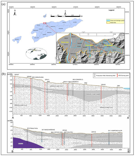
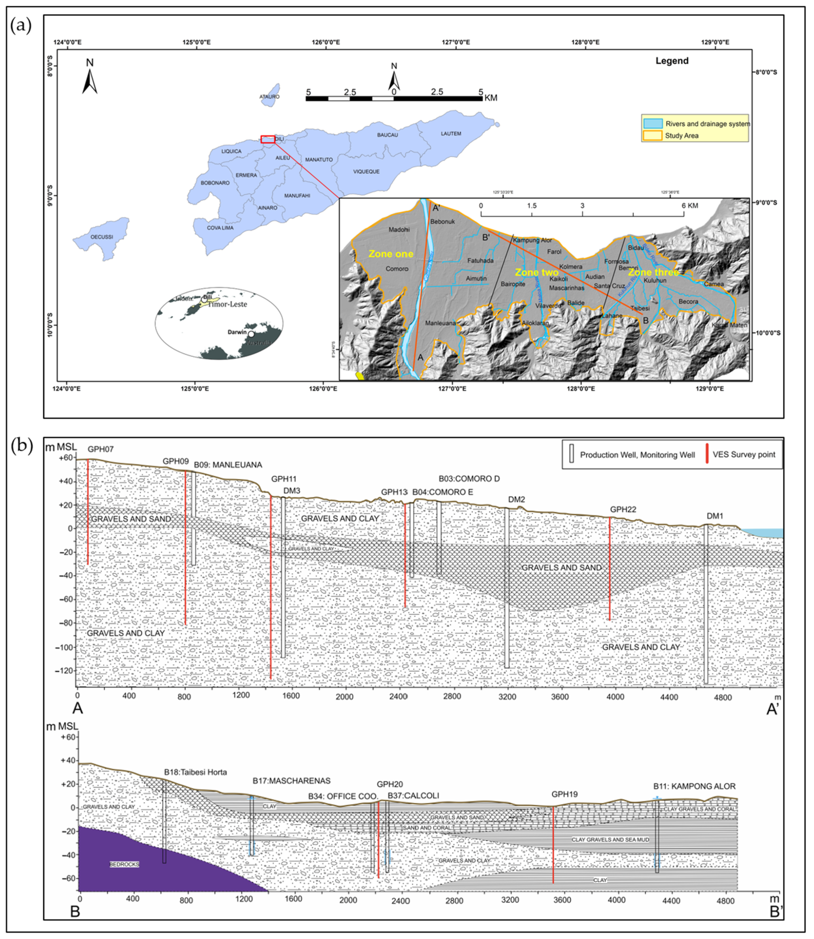
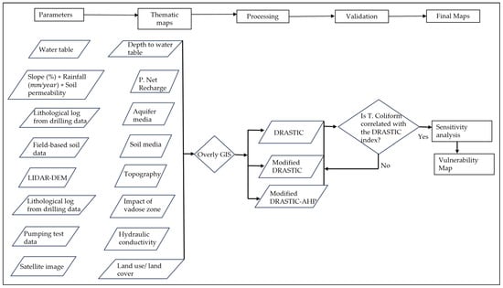
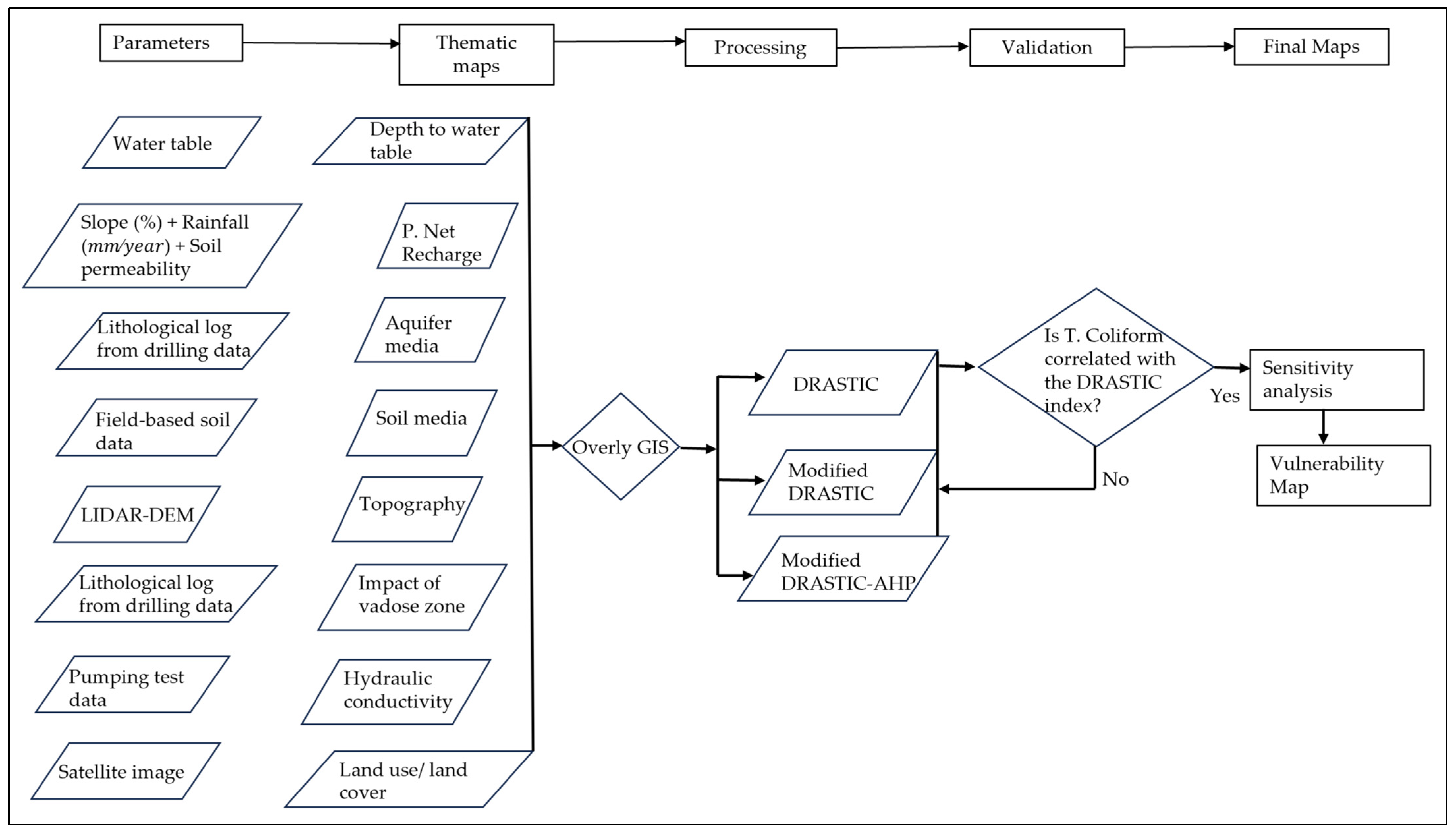
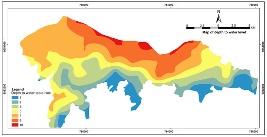
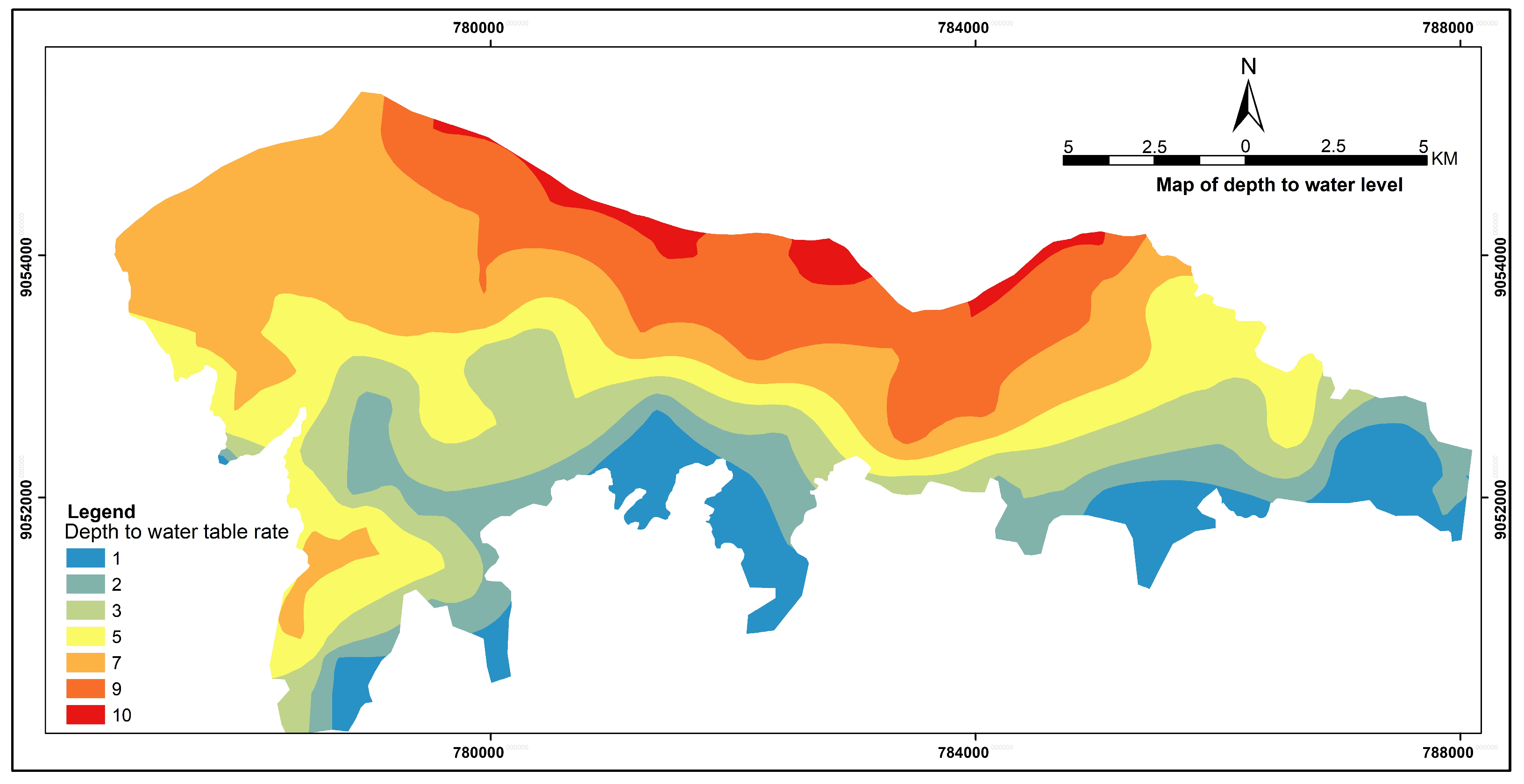
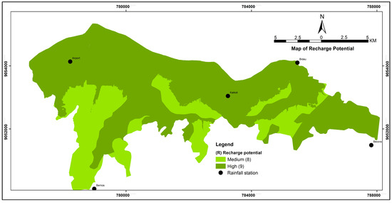
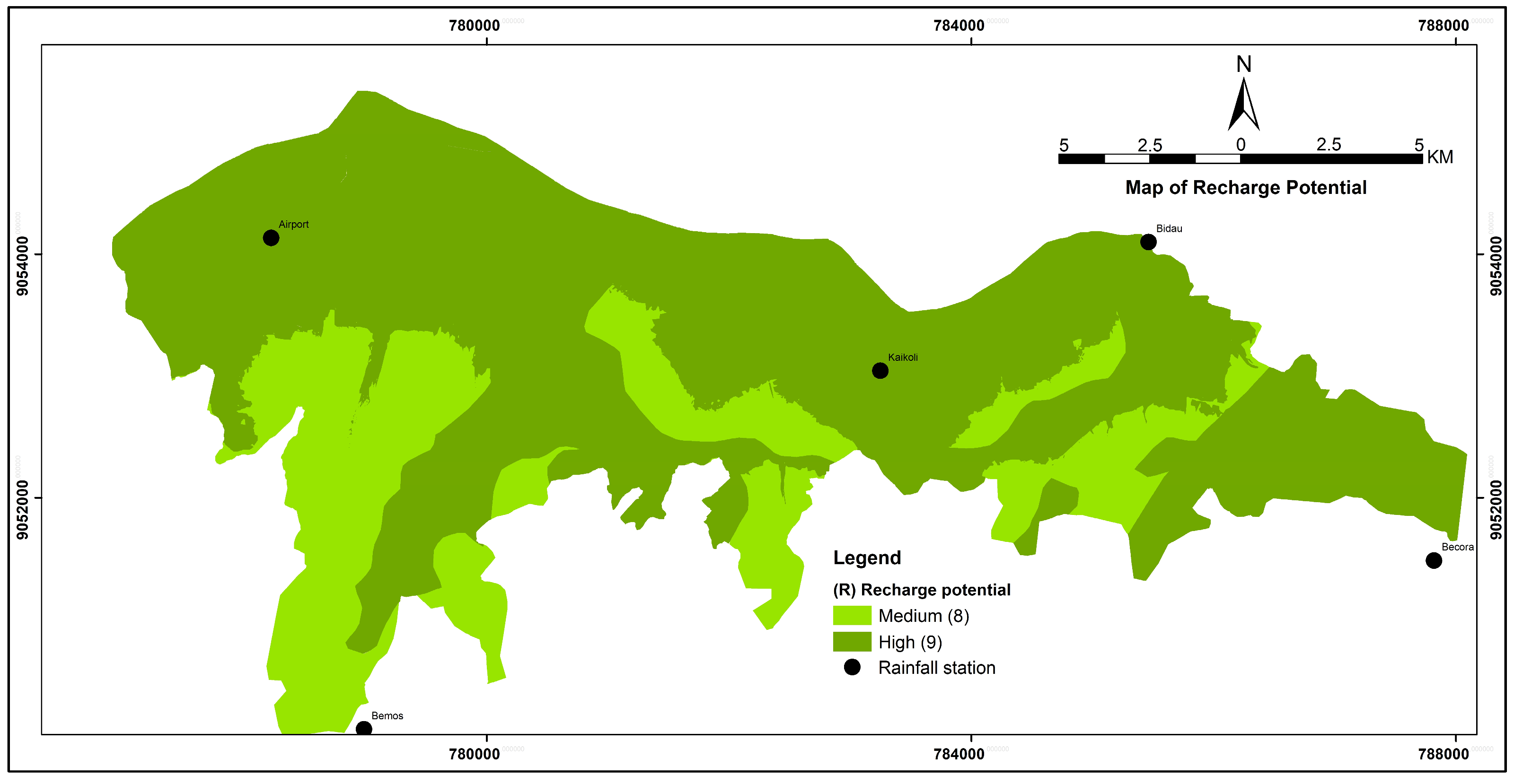
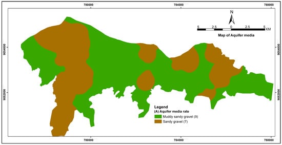
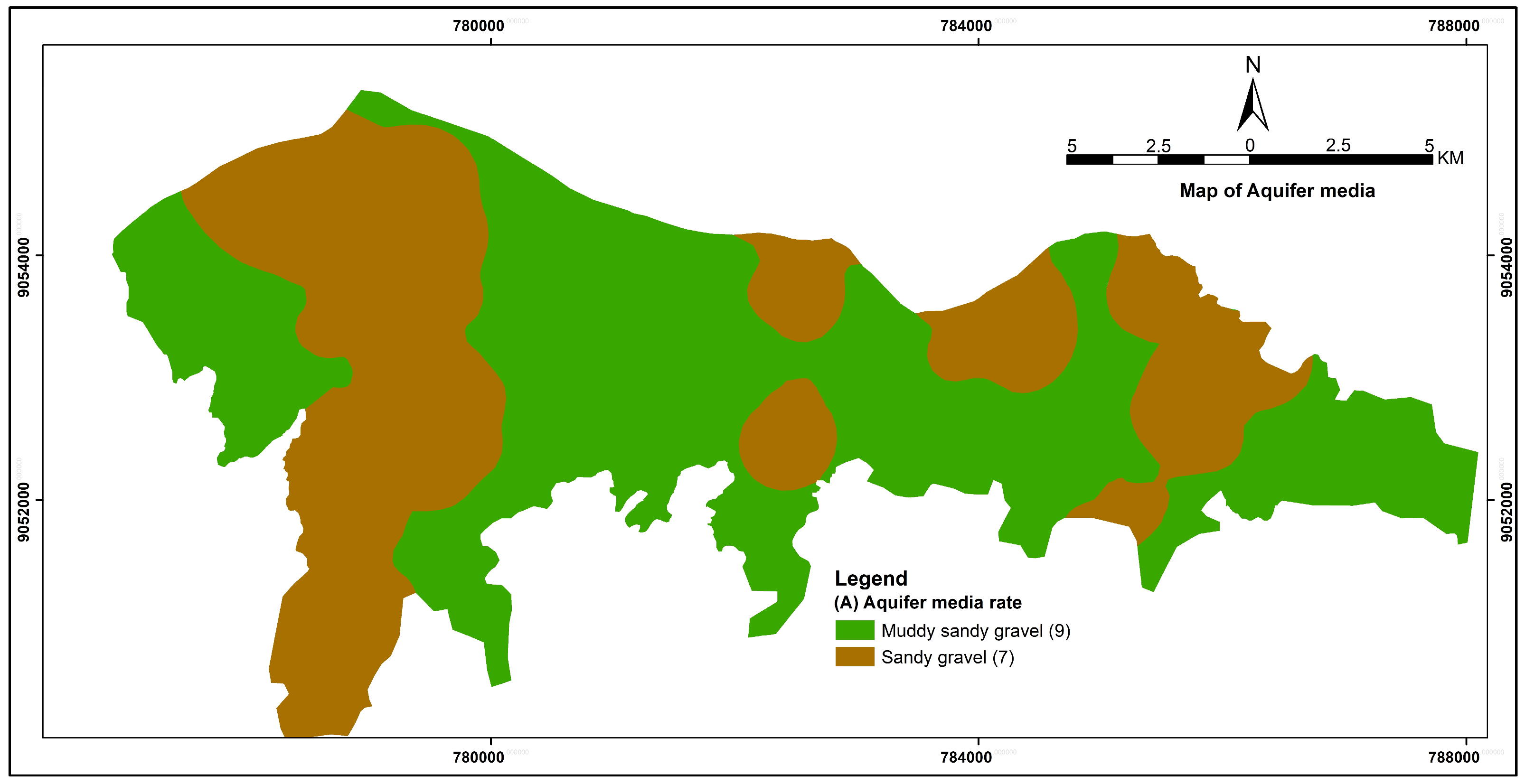
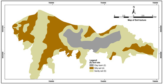
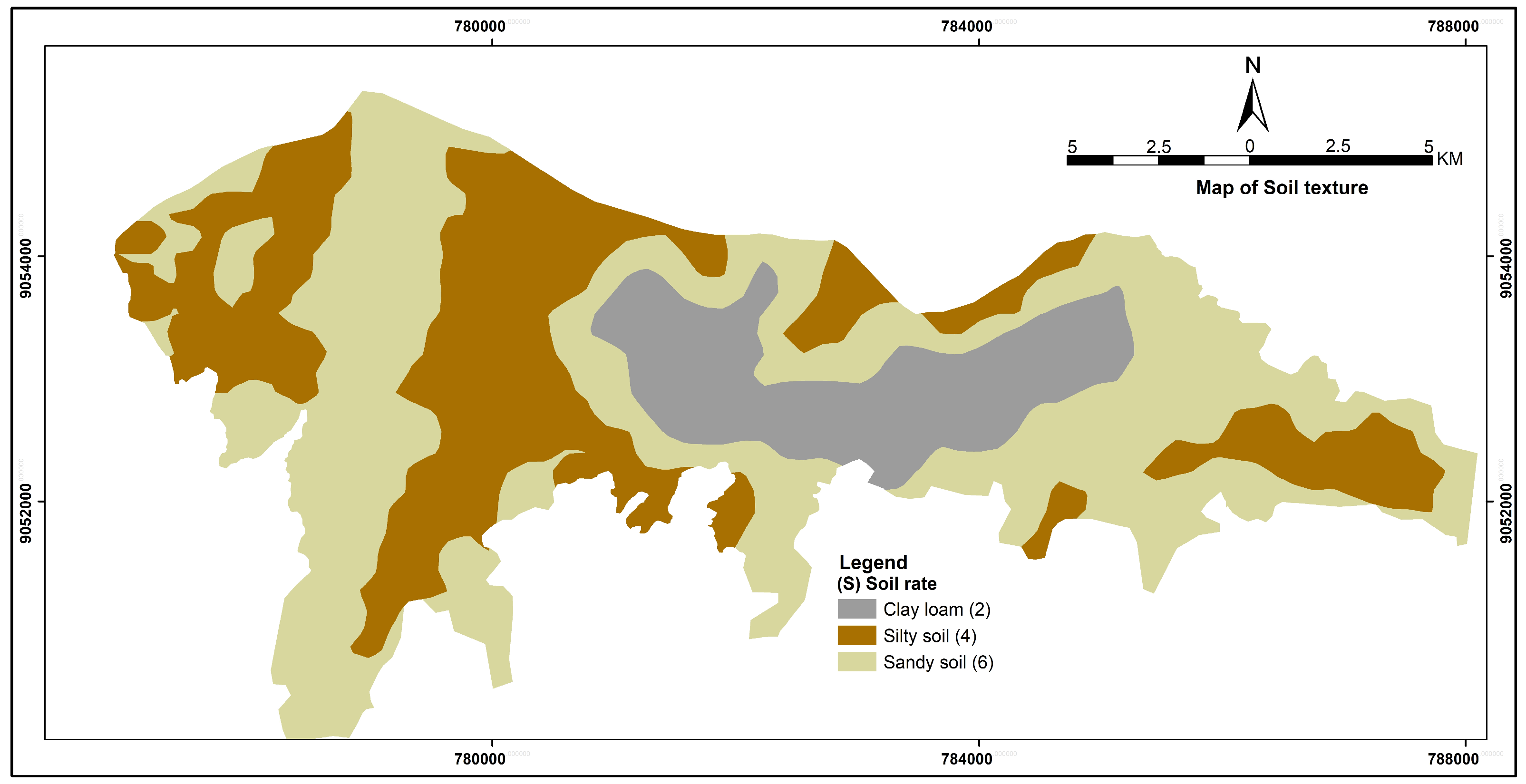
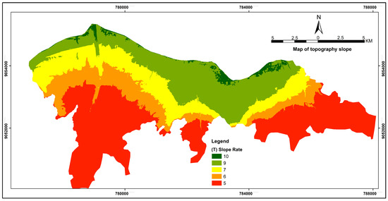
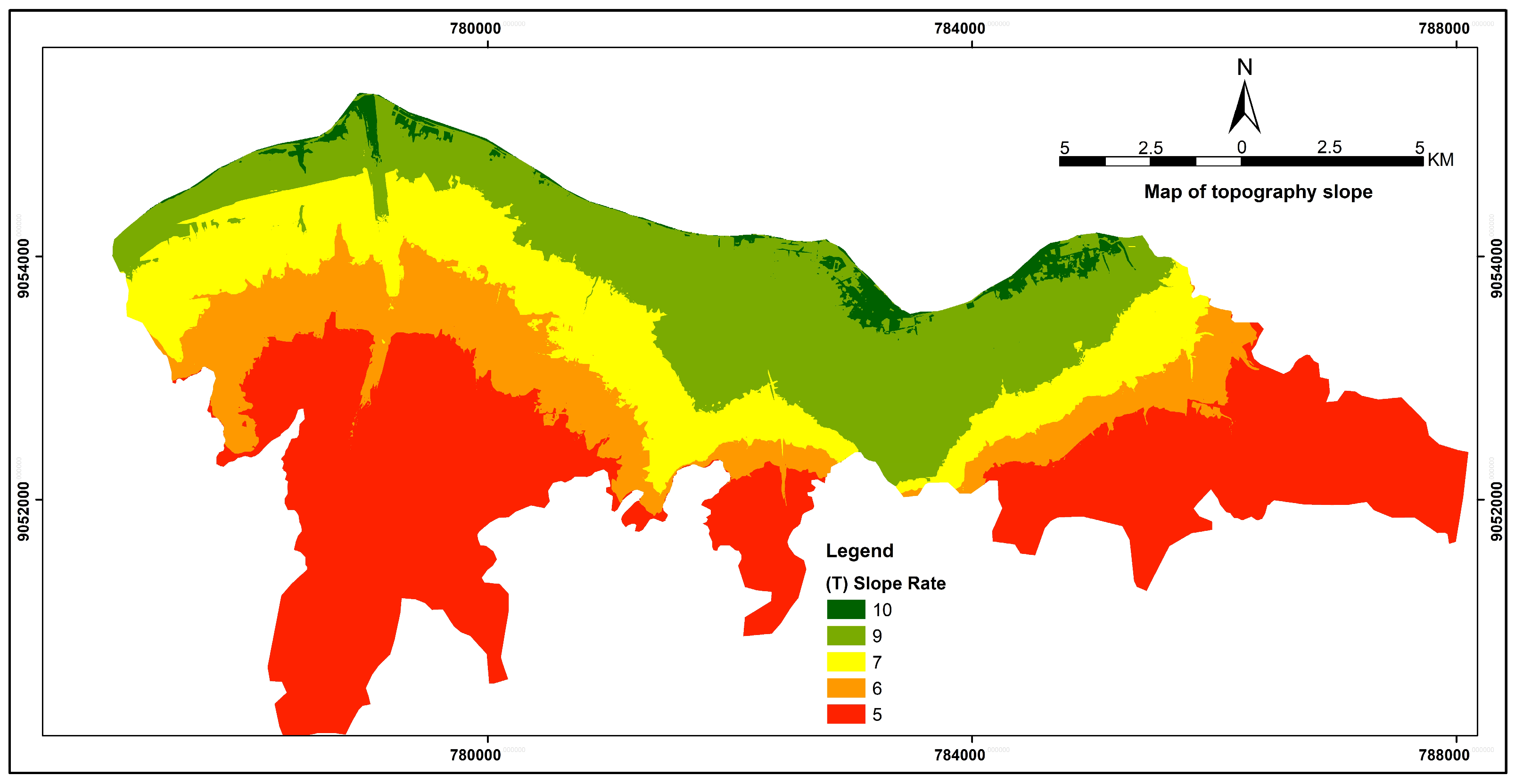
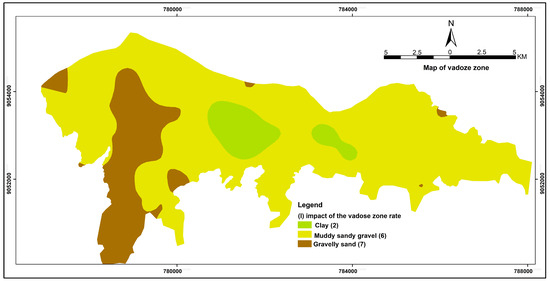
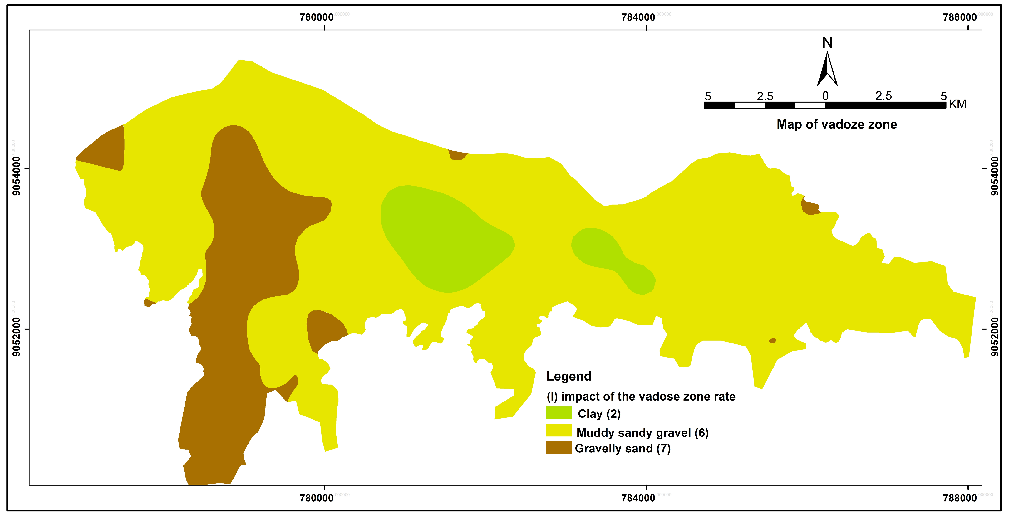
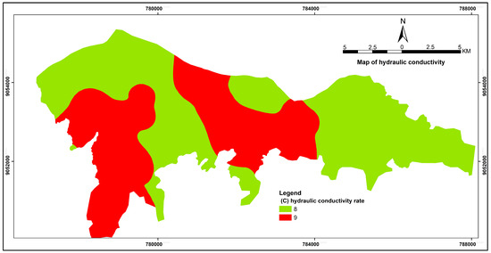
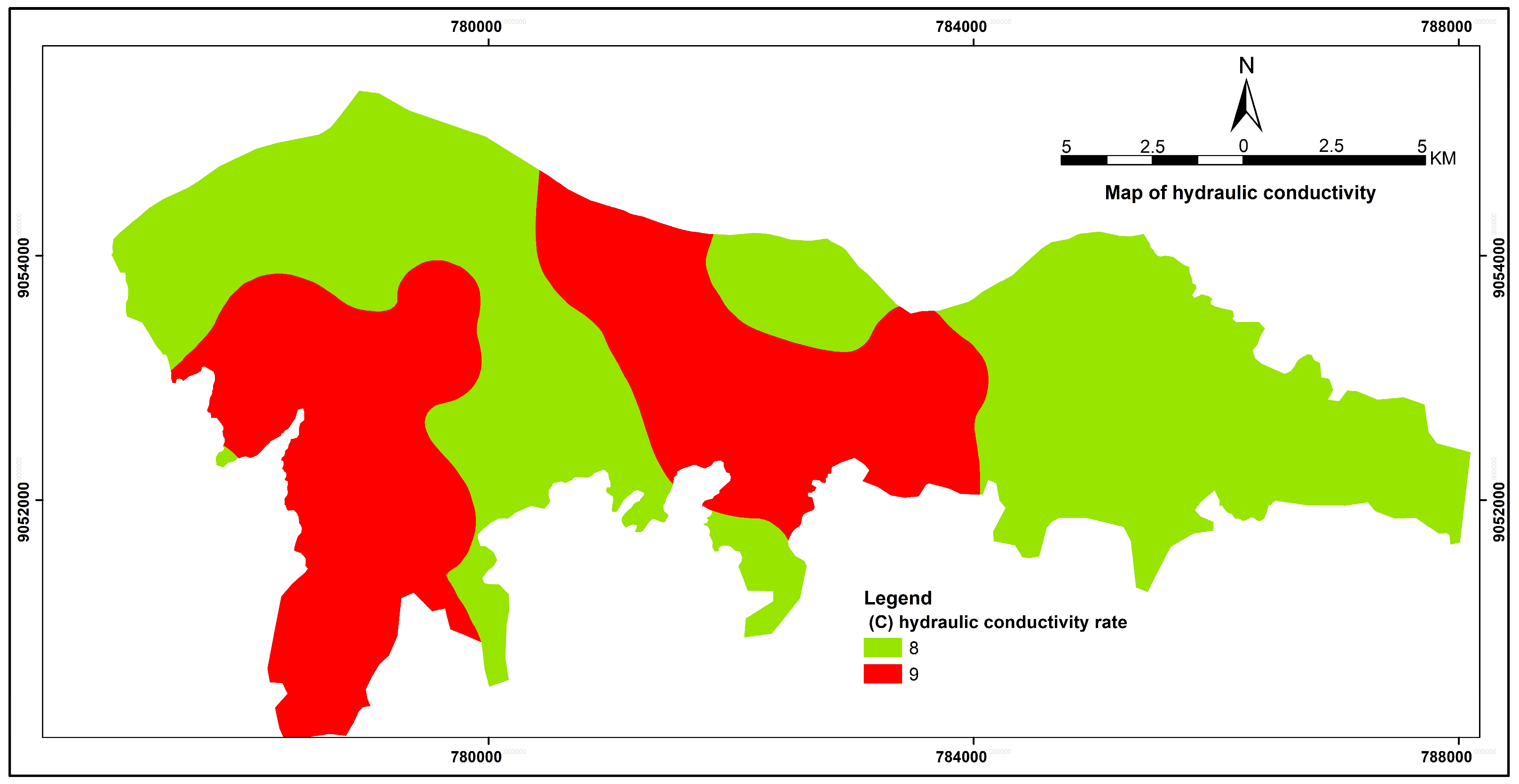
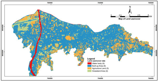
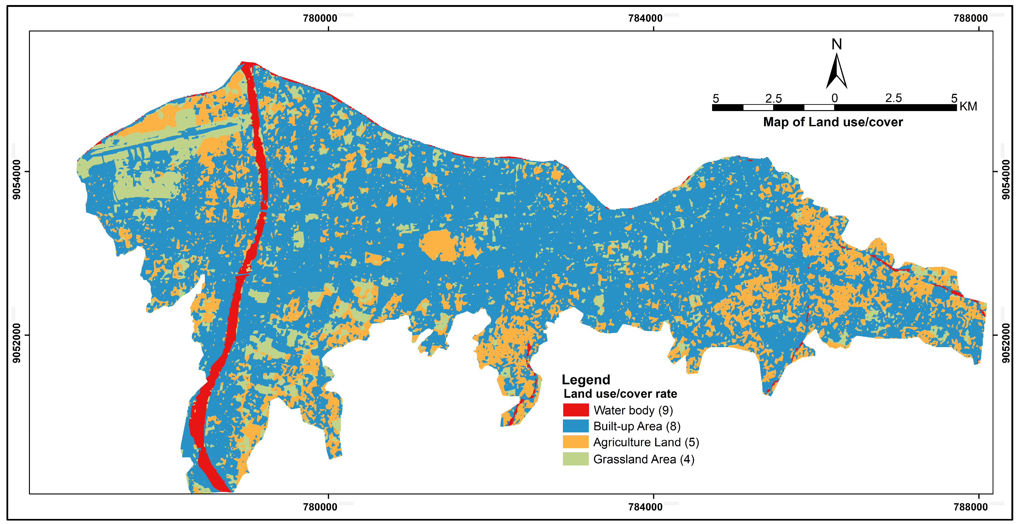
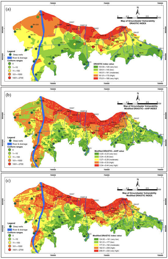
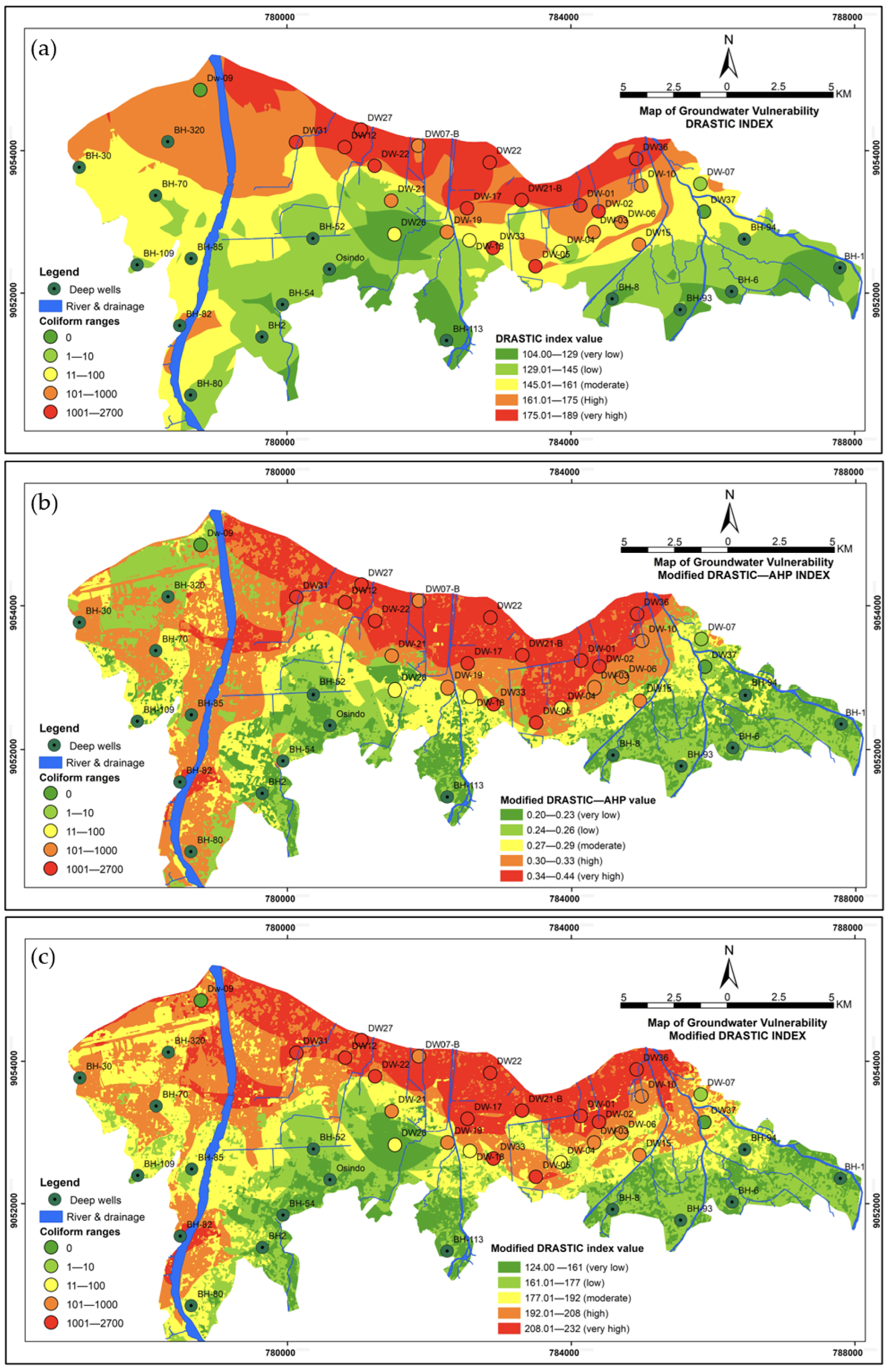
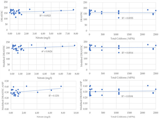
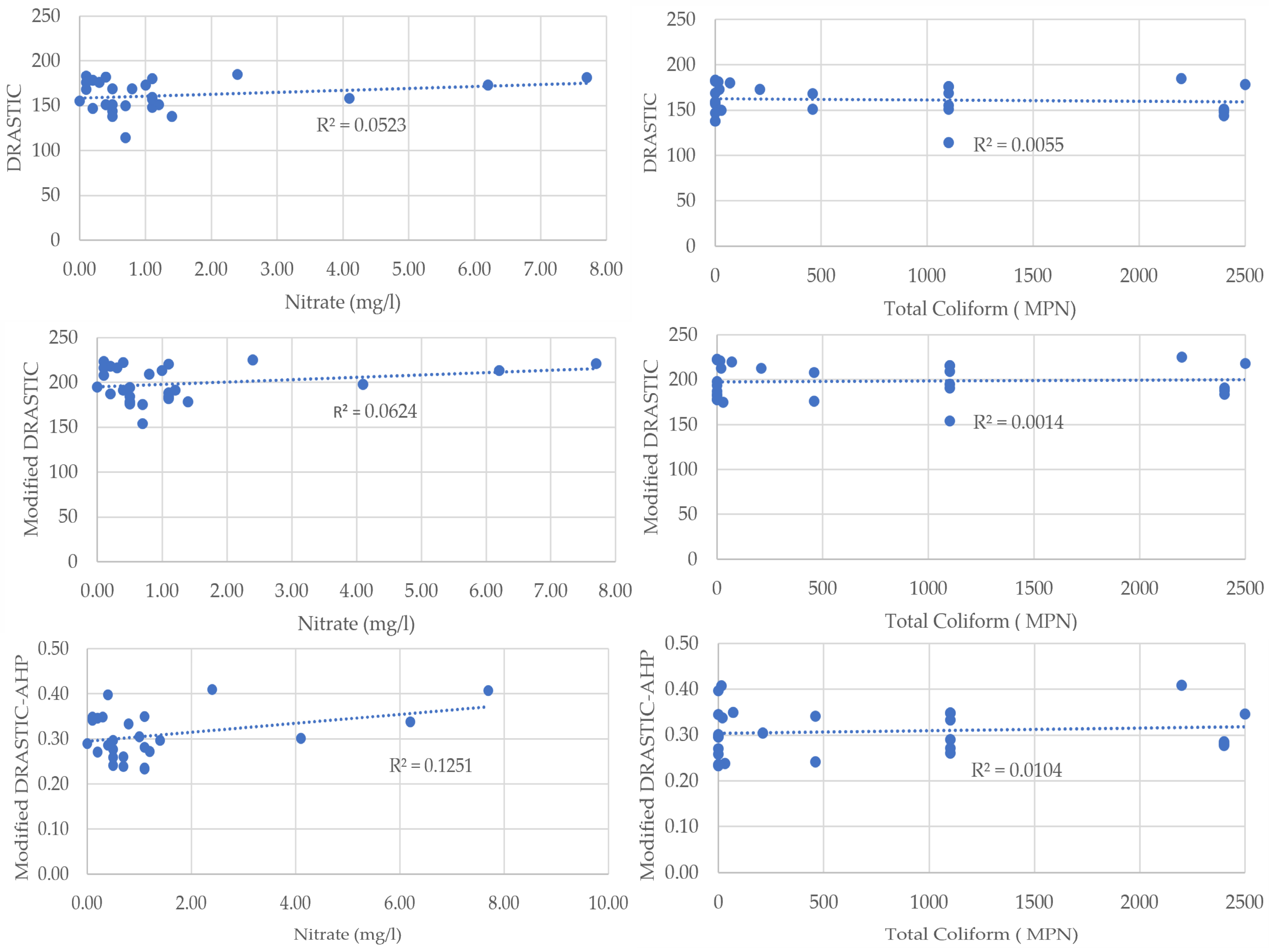
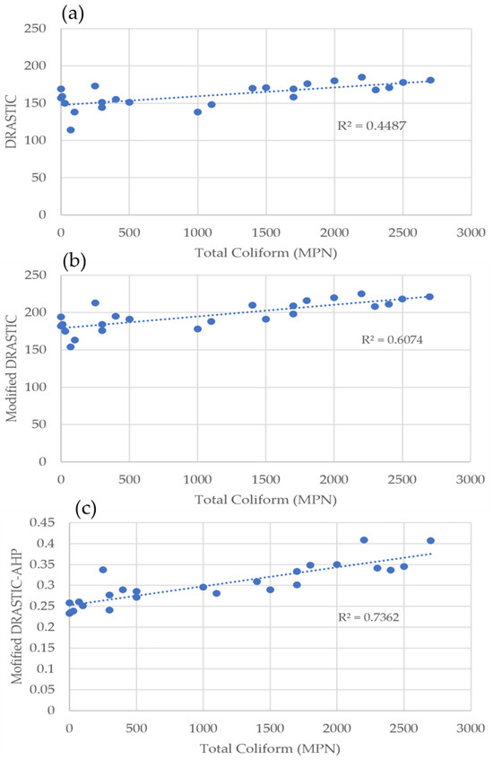
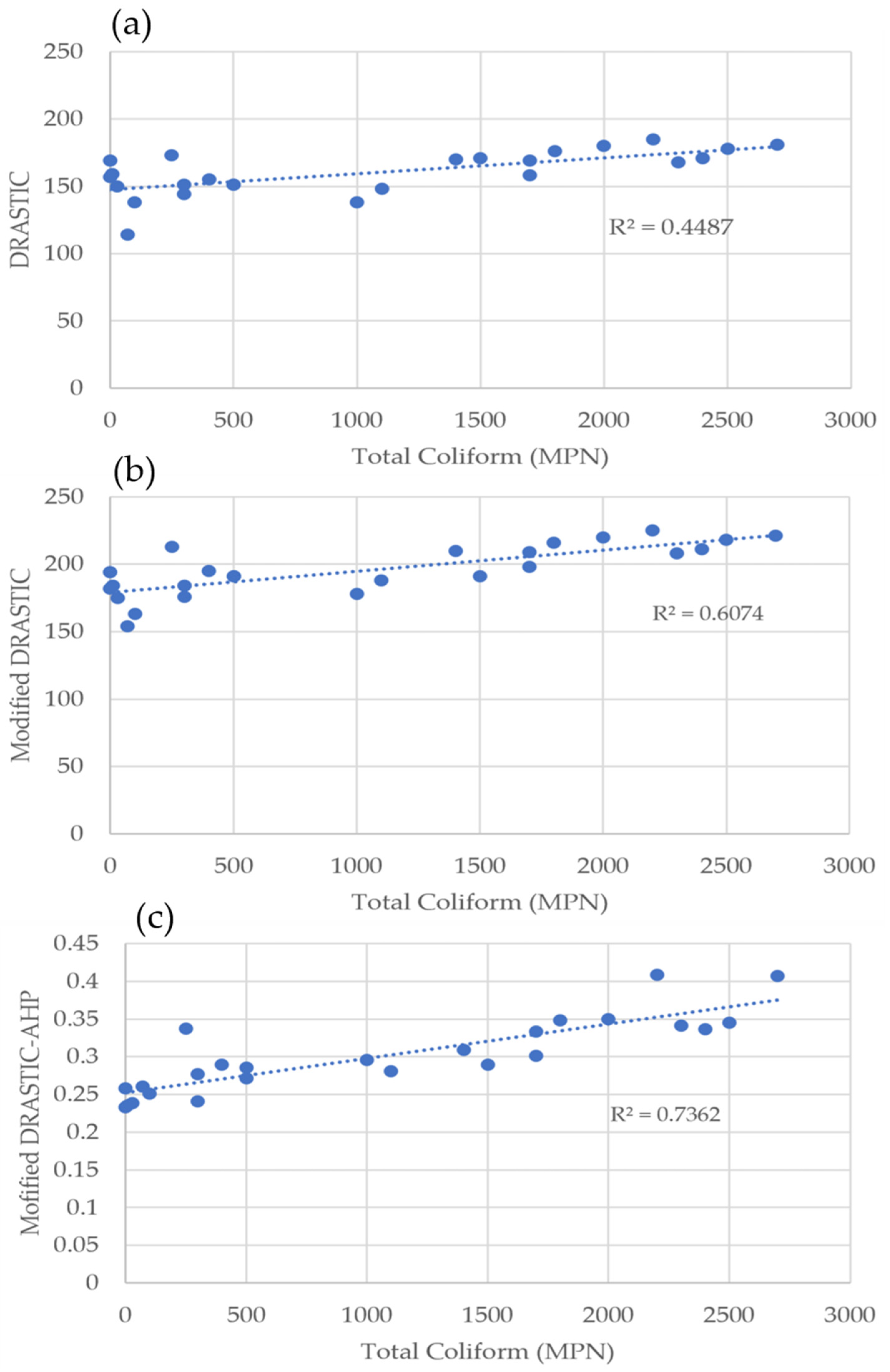
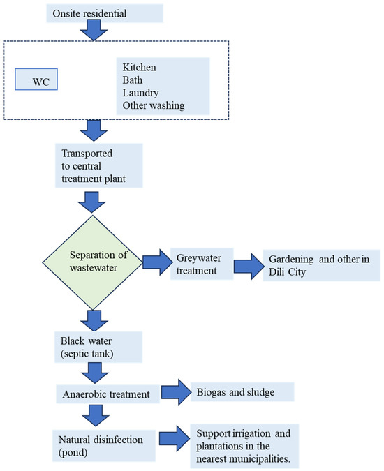
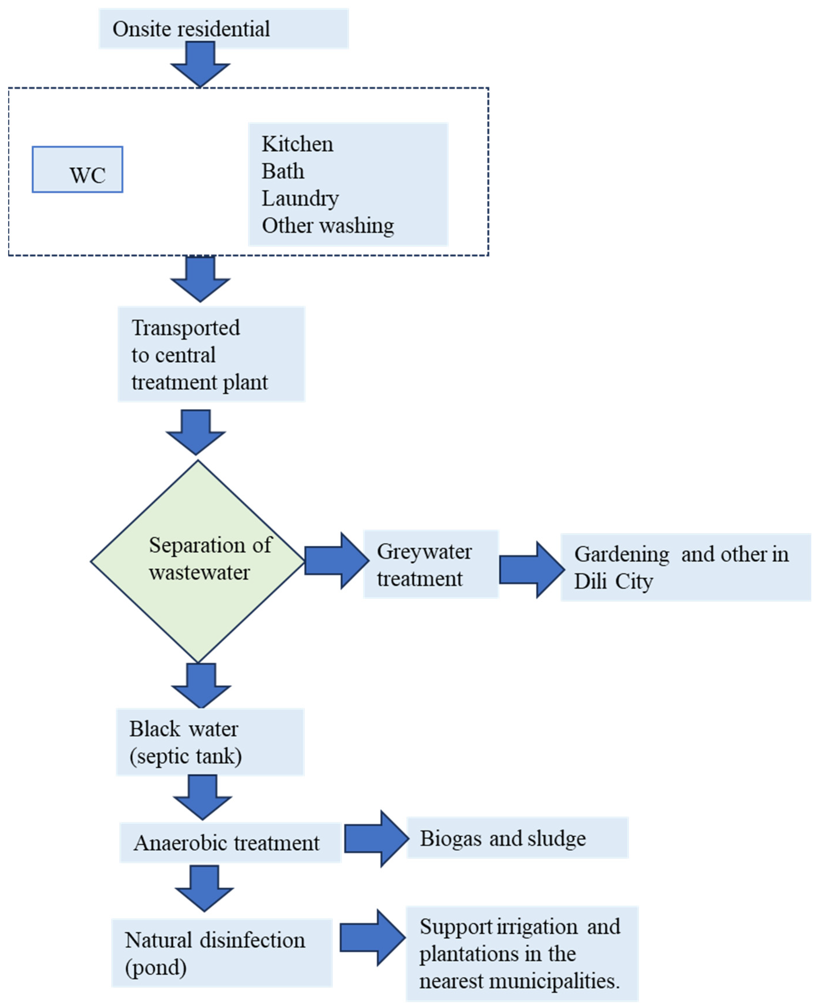

Disclaimer/Publisher’s Note: The statements, opinions and data contained in all publications are solely those of the individual author(s) and contributor(s) and not of MDPI and/or the editor(s). MDPI and/or the editor(s) disclaim responsibility for any injury to people or property resulting from any ideas, methods, instructions or products referred to in the content. |
© 2026 by the authors. Licensee MDPI, Basel, Switzerland. This article is an open access article distributed under the terms and conditions of the Creative Commons Attribution (CC BY) license.