Enhanced IMERG SPE Using LSTM with a Novel Adaptive Regularization Method

Abstract

Satellite-based precipitation estimates (SPE) provide essential spatial coverage and near real-time availability for hydrological applications but often exhibit systematic biases in regions characterized by complex terrain and strong climatic variability, limiting their reliability for flood-related studies. To address these limitations, this study proposes an Adaptive Regularization framework integrated within a Long Short-Term Memory (LSTM) model to enhance satellite–gauge rainfall fusion beyond conventional optimization strategies. The framework dynamically adjusts learning rate and weight decay during training based on validation performance and overfitting indicators, improving training stability, data efficiency, and model generalization across diverse precipitation regimes. The proposed approach was applied to refine Integrated Multi-satellite Retrievals for Global Precipitation Measurement (IMERG) daily rainfall estimates over the flood-prone east coast of Peninsular Malaysia. Model performance was assessed against ten optimization algorithms using correlation coefficient (CC), mean absolute error (MAE), normalized root mean squared error (NRMSE), percentage bias (PBias), and Kling–Gupta efficiency (KGE). Results show that the Adaptive Regularization framework consistently outperforms all benchmark optimizers, achieving an MAE of 6.87, CC of 0.68, NRMSE of 1.84, and KGE of 0.56. Overall, the proposed framework enhances spatial consistency and robustness across monsoon seasons, offering a scalable solution for improving SPE in flood-prone regions.

1. Introduction

Satellite precipitation estimation (SPE) has revolutionized the monitoring and understanding of precipitation patterns on a global scale [1,2]. By leveraging the wide coverage of weather satellites, SPE provides observations in regions that were previously inaccessible or lacked sufficient ground-based stations. The ability to track remote disaster-prone regions, including those affected by floods and landslides, is of significant importance. It is also crucial for responding to fast weather-changing conditions based on near-real-time satellite data, empowering authorities to mitigate the impact of extreme events. The globally available SPE data facilitates international collaboration in climate research and forecasting for meteorologists and researchers across different regions and countries to study global weather patterns, monitor climate variations, and predict extreme events that transcend borders [3,4,5,6,7,8].

Despite these advantages, SPE faces notable challenges. Its accuracy often falls short of direct ground-based measurements and may exhibit significant biases, especially in areas with complex terrain or dynamic weather conditions [9,10,11]. Improving rainfall estimates is therefore crucial for reliable weather information and disaster management. Numerous previous studies attempt to improve the SPE via bias correction techniques such as linear scaling [12,13], power transformation, and quantile mapping [14]. However, these approaches show limited effectiveness as they only adjust part of statistical data characteristics of the dataset. For example, the simple linear scaling method focuses on adjusting the mean of the dataset, while the power transformation technique corrects the second statistical moment of the frequency distribution, such as coefficient of variation (CV) and standard deviation (SD) [14]. On the other hand, quantile mapping method adjusts the entire distribution quantiles of the dataset to match the observed dataset [15]. Although these conventional methods are straightforward to implement for correcting systematic biases in SPE, each has inherent limitations that restrict their effectiveness. They rely on the assumption that the bias structure remains stationary over time [15,16], and they may produce unrealistic or unrepresentative corrections (either over-fitting or under-fitting) when the reference sample size is small [17].

In recent years, machine learning (ML) and deep learning have emerged as promising approaches for improving the accuracy of SPE [18,19]. These methods can identify complex, non-linear patterns in large datasets, leading to more refined and reliable predictions. One example is the use of multi-layered Recurrent Neural Network (RNN) architectures that incorporate feedforward concepts [20]. Among these, the Long Short-Term Memory (LSTM) network is one of the most widely applied models for enhancing SPE performance and in streamflow predictions, with successful implementations demonstrated in previous studies [21,22,23,24]. Despite their capabilities, these models require careful training as deep learning architectures often involve large parameter sets and complex loss landscapes. Beyond model structure, their predictive skill largely depends on the learning dynamics during training, which govern how the model adjusts its parameters in response to errors.

Training these models effectively is crucial to achieving high predictive performance, as their accuracy depends on how well the model parameters are optimized. A key factor in training ML models is the choice of optimizer, which determines how parameters are updated to minimize prediction errors. Broadly, commonly used optimizers can be categorized into three groups: gradient descent-based methods (e.g., Stochastic Gradient Descent, SGD), adaptive learning rate methods (e.g., Adagrad, Adadelta, RMSprop), and momentum-based adaptive methods (e.g., Adam and its variants) [25,26,27,28,29]. Gradient descent-based methods such as SGD are computationally efficient and provide stable convergence; however, they often suffer from slow convergence and sensitivity to learning rate selection, particularly in complex, high-dimensional problems. Adaptive learning rate methods, including Adagrad and RMSprop, address this limitation by scaling updates based on historical gradients, thereby improving convergence in non-stationary settings, although they may exhibit aggressive or diminishing learning rates over time [30,31]. Momentum-based adaptive optimizers such as Adam combine the advantages of momentum and adaptive learning, enabling faster convergence and improved performance in many deep learning applications. However, they have been reported to exhibit generalization issues and may converge to suboptimal solutions under certain conditions [32,33].

Despite these advancements, existing optimizers are generally designed for generic optimization tasks and do not explicitly account for the strong non-linearity, non-stationarity, and spatiotemporal heterogeneity inherent in precipitation processes, which can introduce substantial uncertainties in rainfall estimation processes [2,34]. Data quality issues, such as noise and missing values, and the computational demands of high-dimensional models further complicate optimization [35]. Overfitting is also a key concern and requires the application of appropriate regularization techniques to mitigate its effects and improve model generalizability [36]. Furthermore, conventional regularization approaches, such as dropout and L1/L2 weight decay, often show limited effectiveness in recurrent architectures. In particular, standard dropout may disrupt temporal dependency structure of recurrent neural networks, leading to suboptimal performance when applied directly to LSTM models [37]. Similarly, standard L2 regularization has been reported to exhibit diminished regularization effects when coupled with adaptive optimization due to the interaction between parameter updates and normalization schemes, reducing its ability to control model complexity during training [32,38]. This highlights a clear research gap in developing Adaptive Regularization approach that can dynamically adjust both regularization strength and learning behavior throughout the training process, particularly within LSTM-based SPE correction frameworks.

To improve training stability, enhance data efficiency, and achieve more robust generalization across diverse precipitation regimes, this study introduces an Adaptive Regularization framework to address this limitation by integrating dynamic control of weight decay and learning rates, thereby improving model generalization and stability for LSTM-based satellite precipitation estimation against various optimization methods. The precipitation estimation skills of the Integrated Multi-satellite Retrievals for the Global Precipitation Measurement (IMERG) in the flood-prone states of Pahang, Kelantan and Terengganu (ECPM-PKT), Malaysia, were enhanced using this proposed framework to deliver more precise and reliable rainfall forecasts for the ECPM.

2. Study Area and Data Acquisition

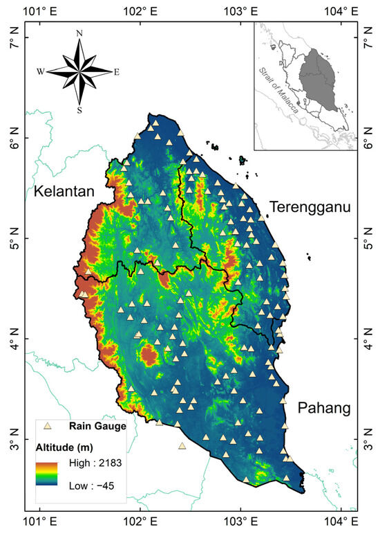
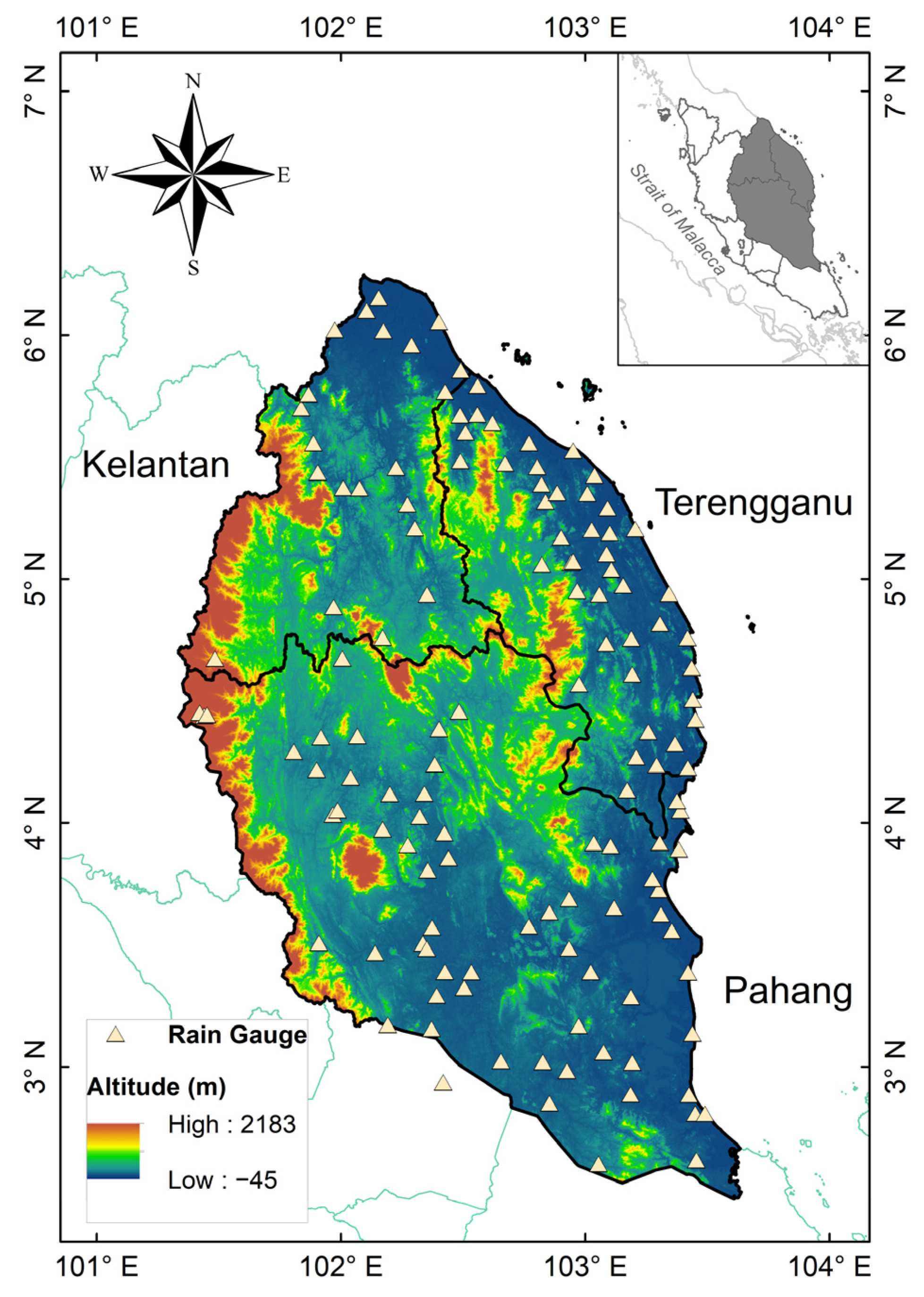
ECPM-PKT (Figure 1) lies between approximately 2–6.5° N latitude and 101–104° E longitude, facing the South China Sea. The region is significantly affected by the Northeast Monsoon (NEM) season, which typically occurs from November to March. Based on the observed records, heavy rainfall occurs predominantly between November and January, consistent with previous studies showing that most extreme precipitation events in Peninsular Malaysia occur during this period [39]. In contrast, the Southwest Monsoon (SWM) season from May to September brings relatively uniform rainfall throughout the season, exhibiting flatter temporal variations with no pronounced peaks. This behavior reflects the generally drier conditions of the SWM season in Peninsular Malaysia, characterized by lower rainfall totals and greater spatial homogeneity [39]. The inter-monsoon (IM) seasons represent the transition periods between the two main monsoon seasons and typically occur in April and October. During the IM season, pronounced rainfall peaks are observed in October, whereas comparatively weaker peaks occur in April.

Figure 1. Study area and the distribution of rain gauge stations. Negative elevation values observed near coastal areas and river channels are attributed to radar signal limitations and interpolation effects in mixed land–water grid cells.

Annual rainfall in the region averages between 2500 and 4000 mm, with pronounced spatial and temporal variability. Combining the high annual rainfall with the region’s low-lying coastal plains and major river basins, such as the Kelantan and Pahang rivers, the ECPM-PKT is highly susceptible to monsoon-driven flooding. This region has experienced several severe flood events, most notably the December 2014 flood in Kelantan, widely regarded as one of the worst floods of the century. This event resulted from prolonged and intense rainfall, which caused major rivers, such as the Kelantan River, to exceed danger levels, leading to widespread inundation and damage [40,41]. Similar flood-prone conditions are also observed in Terengganu and Pahang, where complex river systems, low-lying coastal zones, and monsoonal rainfall contribute to recurrent flooding events. Therefore, the selection of this region provides a suitable testbed for evaluating rainfall estimation performance under hydrometeorological conditions characterized by high variability and extreme events.

In this study, daily rainfall data from 1 January 2011 to 31 December 2020 were obtained from 131 operating rain gauge stations on the ECPM-PKT. These data were provided by the Department of Irrigation and Drainage, Malaysia, and served as reference observations for comparing and enhancing satellite precipitation estimates (SPE). The selected study period was chosen to ensure consistency and reliability within the satellite dataset. Although the IMERG product provides a longer temporal record extending back to 1998 through the Tropical Rainfall Measuring Mission (TRMM) era reprocessing, data prior to 2014 rely on a different satellite constellation and retrospective calibration, which may introduce inconsistencies due to variations in sensor characteristics and retrieval algorithms. Therefore, the 2011–2020 period was adopted to minimize such heterogeneities while still providing a sufficiently long record for robust statistical analysis and capturing both the late TRMM and early Global Precipitation Measurement eras.

Satellite-based precipitation data for the same period were acquired from the IMERG dataset via the Goddard Earth Sciences Data and Information Services Centre (GES DISC) [42]. There are three types of IMERG satellite estimations (Early, Late, and Final) and available with half-hourly, daily, and monthly temporal resolutions. In this study, the IMERG Final version (IMERG-F) daily version 6 product at a spatial resolution of 0.1° is bias-corrected using the Global Precipitation Climatology Centre (GPCC) precipitation gauges and is suitable for scientific research; thus, it is more accurate compared to other IMERG products [2].

The differences between satellite-based precipitation estimates and gauge-based observations should be interpreted in light of the inherent uncertainties in both datasets. Rain gauge measurements are commonly treated as reference data due to their direct observation of rainfall at specific locations. However, they are subject to limitations such as spatial representativeness, measurement errors (e.g., wind-induced undercatch), and uneven station distribution, particularly in complex terrain. In contrast, satellite-based products provide broader spatial coverage but may be affected by retrieval uncertainties related to cloud structure, topography, and algorithm assumptions. In this study, gauge observations are used as the reference for evaluation. However, discrepancies between the two datasets do not necessarily indicate errors solely in the satellite estimates. Therefore, the evaluation focuses on the relative performance and consistency of the satellite-based estimates in capturing temporal variability and spatial patterns, rather than absolute agreement alone.

3. Materials and Methods

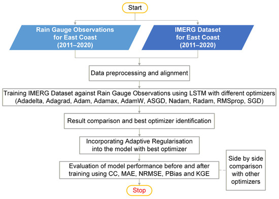
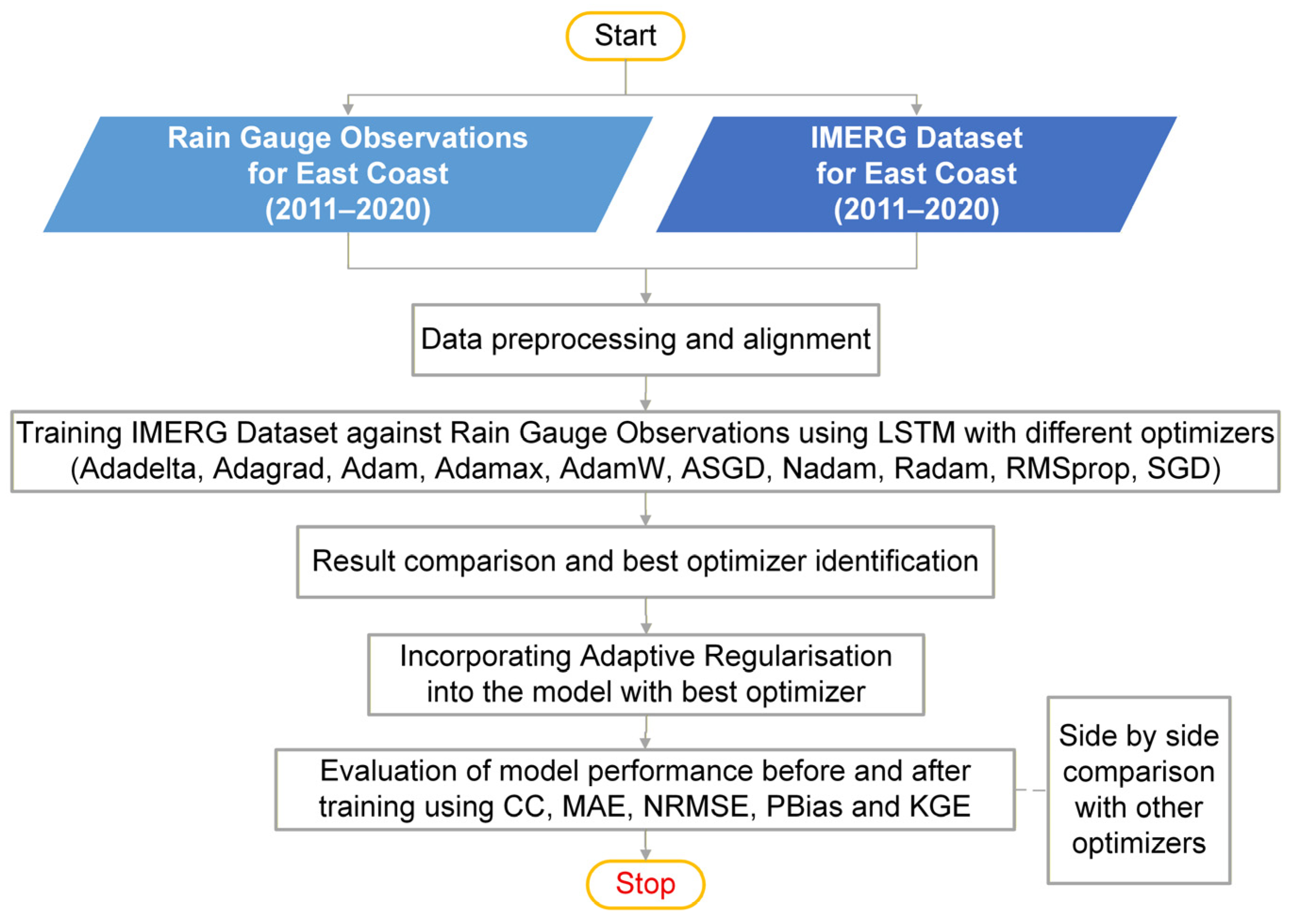
A robust methodology has been formulated to refine satellite-derived IMERG rainfall estimates by integrating ground-based rain gauge observations, with a specific focus on the ECPM-PKT. The approach leverages LSTM deep learning models, systematically evaluates various optimizers, and introduces a novel Adaptive Regularization framework. The overall research workflow is depicted in Figure 2.

Figure 2. IMERG data enhancement with different optimizers and Adaptive Regularization.

3.1. Data Preprocessing and Alignment

Rigorous data preprocessing and alignment were performed to ensure the data’s quality and compatibility to be used for deep learning model training. Both IMERG and rain gauge data are loaded in a comprehensive database system. As the datasets are large, comprehensive quality control procedures were applied to identify and handle missing values, outliers, and any erroneous readings that could negatively impact model performance.

Precise temporal alignment is crucial, ensuring that IMERG estimates correspond directly to rain gauge observations for the same time intervals (e.g., hourly, daily) to achieve temporal synchronization. Given IMERG’s half-hourly updates, the data were aggregated and synchronized with hourly rain gauge observations. Structured Query Language (SQL) was used within the RDS to perform sophisticated data manipulation.

As rain gauge data are point observations and IMERG data are gridded, a spatial matching strategy is implemented for spatial alignment. This involves normalization and splitting of data. To optimize the deep learning training process, both input (IMERG) and target (rain gauge) data are scaled using min-max normalization. This is to ensure variables with bigger magnitudes do not disproportionately influence the learning algorithm.

Lastly, the preprocessed dataset was chronologically divided into three sets: training, validation, and test, with proportions of 70%, 15%, and 15%, respectively. The training set was used to fit the model parameters, the validation set was used to adjust hyperparameters and monitor overfitting during training, and the test set was reserved for final, unbiased evaluation. This chronological split was essential to prevent data leakage and to ensure that model performance was evaluated on truly unseen future data.

3.2. Baseline LSTM Training and Optimizer Selection

The initial phase of the methodology involves training the LSTM model with a variety of optimizers to establish a performance baseline and identify the most suitable optimizer for the rainfall prediction task. The LSTM model of “peephole connections” variant was used to train the IMERG rainfall data against rain gauge observations. The LSTM’s inherent capability to capture long-term dependencies is particularly crucial for effectively modeling the sequential nature of rainfall time series data [43].

The LSTM model was independently trained using a comprehensive set of optimizers: Adadelta, Adagrad, Adam, Adamax, AdamW, ASGD, Nadam, Radam, RMSprop, and SGD. This systematic comparison aims to assess their respective convergence speed, stability, and initial generalization performance on the rainfall dataset. The root mean squared error (RMSE) was employed as the loss function in all training runs, providing a robust measure of the average squared difference between predicted and observed rainfall values [44]. Following the training with each optimizer, model performance was evaluated on the validation set using the RMSE. Based on this comparative analysis, the best-performing optimizer is identified and subsequently used for further training with the Adaptive Regularization framework.

3.3. Adaptive Regularization Framework with LSTM and Best-Performing Optimizer

The core novelty of this research is the proposed Adaptive Regularization framework, which is applied to the LSTM model utilizing the identified best optimizer. This framework dynamically adjusts key training hyperparameters, specifically weight decay and learning rate, during the training process. By adapting these parameters, the framework mitigates overfitting and improves the model’s ability to generalize to unseen data.

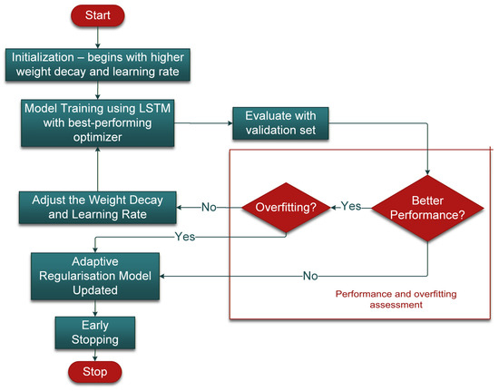
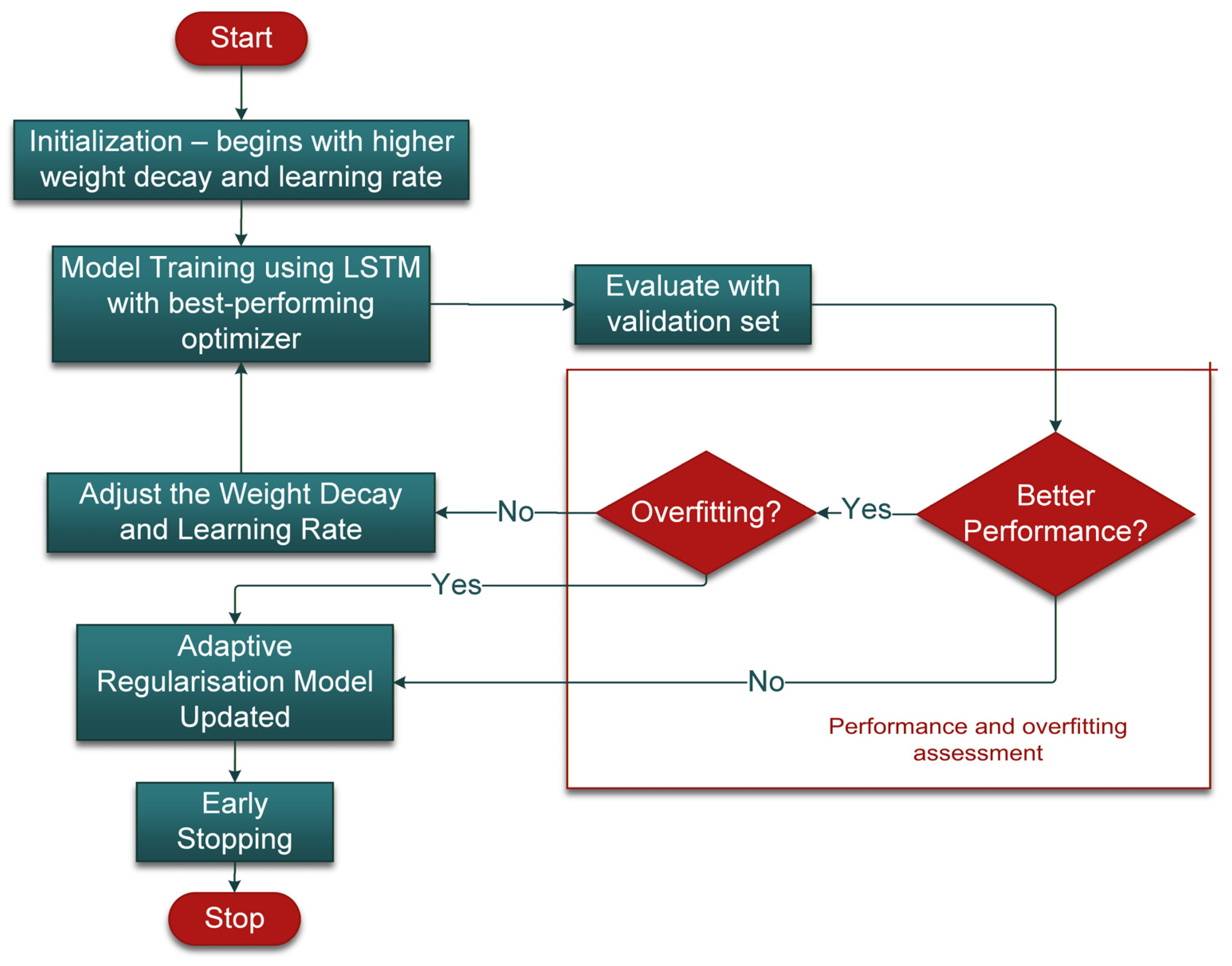
The training procedure for the Adaptive Regularization framework proceeds through a series of adaptive stages, each involving specific updates to learning rate and weight decay, as described in the following section. The Adaptive Regularization process consists of seven main stages (Figure 3).

Figure 3. Proposed Adaptive Regularization flowchart.

Stage 1: Initialization. The training begins with a predefined set of initial hyperparameters for weight decay and learning rate. These initial values are chosen to allow rapid early exploration of the parameter space.

Stage 2: Model Training using LSTM and best-performing optimizer. The LSTM model is trained using the best-performing optimizer. Its decoupled weight decay is essential because it applies regularization independently from adaptive learning rate updates, allowing consistent and predictable control of regularization within the adaptive framework.

Stage 3: Evaluation with Validation Set. After each training epoch (or after a fixed number of iterations), the model’s performance is rigorously evaluated on an independent validation set. Metrics such as the validation loss (e.g., RMSE) are continuously monitored.

Stage 4: Performance and Overfitting Assessment. The model’s validation performance is compared across epochs to detect improvement or degradation. At the same time, overfitting is explicitly assessed by monitoring the divergence between training and validation losses. A widening gap—where training loss decreases while validation loss plateaus or increases—signals overfitting.

Stage 5: Adjustment of Weight Decay and Learning Rate. Based on the validation results and overfitting indicators, the weight decay and learning rate are dynamically adjusted. If the validation loss worsens or overfitting is detected, the weight decay is increased to impose stronger regularization, while the learning rate is reduced to promote more cautious updates. Conversely, if performance remains stable with no overfitting signs, the learning rate may be maintained or slightly increased to accelerate convergence, and weight decay adjusted to prevent underfitting. This adaptive logic, which continuously tunes regularization (weight decay) and optimization (learning rate) parameters based on model behavior on unseen data, forms the core of the proposed Adaptive Regularization method.

Stage 6: Adaptive Regularization Model Update. The model parameters are then updated using the newly adjusted hyperparameters, and the training loop continues.

Stage 7: Early Stopping. Finally, an early stopping mechanism is applied. Training is halted if validation performance fails to improve for a predefined number of consecutive epochs (patience), or if signs of memorization and overfitting are observed. This ensures computational efficiency and selection of a generalizable model.

3.4. Performance Evaluation and Comparative Analysis

The performance of the trained LSTM model with the Adaptive Regularization framework was rigorously evaluated on the independent test set using a comprehensive suite of statistical metrics commonly employed in hydrological and meteorological studies. Several statistical indicators were used to evaluate model performance, including the Correlation Coefficient (CC), Mean Absolute Error (MAE), Normalized Root Mean Squared Error (NRMSE), Percentage Bias (PBias), and Kling–Gupta Efficiency (KGE). Among these, only the PBias and KGE equations are presented below, as the other indicators are well established and widely recognized in hydrological and machine learning studies.

PBias quantifies the average tendency of the predicted values to be larger or smaller than their observed counterparts. It is calculated as:

$$PBias=\left({\displaystyle \frac{{\sum }_{i=1}^n{S}_i}{{\sum }_{i=1}^n{G}_i}}-1\right)\times 100\%,$$

(1)

where S_i and G_i denote the simulated and observed values, respectively, and n is the number of observations. A positive PBias indicates overestimation, whereas a negative value indicates underestimation.

KGE provides a comprehensive evaluation of model performance by combining correlation, bias, and variability components [45]. It is defined as:

$$KGE=1-\sqrt{{(r-1)}^2+{(\alpha -1)}^2+{(\beta -1)}^2},$$

(2)

where r represents the correlation coefficient between simulated and observed data; α is the variability ratio, and β is the bias ratio (the ratio of their mean values).

The combination of these indicators—CC, MAE, NRMSE, PBias, and KGE—provides a robust assessment of the model’s accuracy, consistency, and predictive reliability. The evaluation involved two key comparisons: Comparison before and after Adaptive Regularization and side-by-side comparison with other optimizers. The performance of the LSTM model trained with best-performing optimizer without Adaptive Regularization was compared against the performance of the LSTM model trained with best-performing optimizer with the proposed Adaptive Regularization framework. This comparison quantifies the improvement gained by the Adaptive Regularization method using the specified metrics (CC, MAE, RMSE, PBias, KGE).

The final optimized LSTM model, incorporating the best-performing optimizer and the Adaptive Regularization framework, was compared against the baseline LSTM models trained with other optimizers established in Phase 1. This comprehensive evaluation demonstrated the effectiveness and superiority of the proposed approach in satellite–gauge rainfall data fusion for the ECPM-PKT.

3.5. Long Short-Term Memory (LSTM)

The standard LSTM architecture has memory blocks in the recurrent hidden layer that contains gates to control the information flow [46]. The three types of gates (forgotten gate, input gate and output gate) are the memory cells that remember the state in the network. The forgot gate will reset the cell states from the beginning and scale the internal state of the cell before adding to cell input. The flow of input and output activations will be controlled by input gate and output gate respectively [47]. The proposed LSTM algorithm contains peephole connections that let the gate layers consider the cell state [48]. Equations (3)–(8) were used to compute a mapping from the input sequence (x) to output sequence (y) iteratively with time (t) for the LSTM algorithm used.

$$i_t=\sigma (W_{ic}{c}_{t-1}+W_{ih}{h}_{t-1}+W_{ix}{x}_t+b_i),$$

(3)

$$f_t=\sigma (W_{fc}{c}_{t-1}+W_{fh}{h}_{t-1}+W_{fx}{x}_t+b_f),$$

(4)

$$o_t=\sigma (W_{oc}{c}_{t-1}+W_{oh}{h}_{t-1}+W_{ox}{x}_t+b_o),$$

(5)

$$c_t=f_t\odot c_{t-1}+i_t\odot \mathit{tanh}(W_{ch}{h}_{t-1}+W_{cx}{x}_t+b_c),$$

(6)

$$h_t=o_t\odot \mathit{tanh}\left(c_t\right),$$

(7)

$$y_t=W_{yh}{h}_t+b_y,$$

(8)

where i_t, f_t, and o_t denote the input, forget, and output gates at time step t, respectively; c_t and h_t represent the cell state and hidden state, while x_t and y_t are the input and output vectors. The matrices W and vectors b correspond to weights and biases. The functions σ(⋅) and tanh(⋅) denote the sigmoid and hyperbolic tangent activations, respectively, and ⊙ indicates element-wise multiplication. The formulation of these gating mechanisms and state transitions follows the standard LSTM architecture described in previous studies [49,50].

3.6. Optimization

PyTorch (Version 2.2.0) optimizers are an essential component of deep learning algorithms. They are responsible for optimizing the performance of neural networks by adjusting the weights and biases during the training process. PyTorch provides a wide range of optimizers that can be used to optimize the performance of neural networks. In this article, we explored the most used PyTorch optimizers such as SGD, Adam, Adagrad, Adadelta, and RMSprop, and discussed their working principles and strengths. Choosing the right optimizer depends on various factors such as the complexity of the problem, the size of the dataset, and the type of neural network architecture. The 10 different optimizers used in this research are summarized in Table A1.

3.7. Regularization

Although choosing the right optimizer is important, there is a need for an effective regularization method to improve data efficiency during training and to prevent the overfitting of the LSTM model. Dropout is a technique that prevents overfitting and provides a way to combine different neural network architectures efficiently [51]. L2 regularization, also called weight decay, is also used to prevent overfitting. The objective function of a neural network with L2 is a combination of an unregularized objective and a regularization term.

3.8. Adaptive Regularization

Simply applying dropout to an LSTM model does not work well, as it might disrupt the nature of the RNN [52]. Study shows that L2 regularization has no regularization effect when combined with normalization [32]. From our previous training results, we found out that LSTM model trained with optimizer with regularization outperformed those without regularization [42]. Motivated by this observation, we further improve the training process using a proposed Adaptive Regularization method that trains the IMERG satellite rainfall data with rain gauge observations.

The Adaptive Regularization framework is integrated into the LSTM training process to dynamically adjust key hyperparameters, namely the learning rate and weight decay, based on real-time training and validation feedback. A series of controlled experiments was conducted to examine the influence of weight decay on model generalization and test performance. The training process is initialized with a learning rate of 0.01 and a weight decay of 0.1. During training, both training and validation losses are continuously monitored. The adaptive framework is implemented as an explicit, rule-based update procedure in the epoch-wise PyTorch program, enabling iteratively adjusting both parameters according to the behavior of the loss functions. Through systematic experimentation, multiple update weighting strategies for both parameters were evaluated, and a 30% reduction in both weight decay and learning rate was determined to be the most effective adjustment scheme. Specifically, when the training loss remains high and shows no further improvements, the weight decay is reduced to allow the model to better fit the data and avoid underfitting. To avoid potential overfitting, the reduction in the weight decay is guided by comparing the training loss and the validation loss, ensuring that both remain in the same order of magnitude. In parallel, the learning rate is gradually decreased in conjunction with weight decay adjustments to ensure stable convergence as the model approaches an optimal solution.

This adaptive mechanism operates continuously throughout the training process, using the divergence between training and validation loss as an indicator of model generalization. In addition, an early stopping criterion is implemented to terminate training when validation performance deteriorates, thereby preventing overfitting and unnecessary computation. Through this dynamic tuning strategy, the framework effectively balances bias and variance, enabling improved generalization while maintaining stable and efficient convergence.

To assess the model’s generalization and avoid overfitting or underfitting, performance metrics are reported for both the training and validation datasets (Table A2). Validation results are directly compared with observed data to evaluate how well the model predicts unseen conditions. This comprehensive evaluation indicates that the model maintains consistent performance across datasets, demonstrating robust generalization.

The central innovation of this methodology is the Adaptive Regularization loop, depicted in the provided Figure 3. This loop dynamically controls the training process to optimize for both convergence and generalization. The strategy also dynamically adjusts both weight decay and learning rate based on real-time validation performance and explicit measurements of overfitting. The explicit inclusion of “overfitting measurements” as a trigger for Adaptive Regularization, beyond merely monitoring “better performance”, signifies a refined control mechanism. This approach aims to prevent the onset of overfitting proactively rather than simply reacting to performance plateaus or degradation. Such a proactive adjustment is particularly crucial for time series data, like rainfall, where complex temporal dependencies can lead to intricate overfitting patterns that are difficult to reverse once established.

The overarching objective of this research is to demonstrate that this integrated adaptive approach enhances model generalization and robustness for precipitation estimation, thereby addressing a critical research gap. While LSTMs and the used optimizers are well-established, and various adaptive hyperparameter tuning methods exist, the specific integration of dynamic, performance-driven adjustment of both weight decay and learning rate within a continuous feedback loop for satellite-gauge rainfall fusion represents a potentially novel contribution to the field.

4. Results and Discussions

4.1. Daily Performance of Optimizers

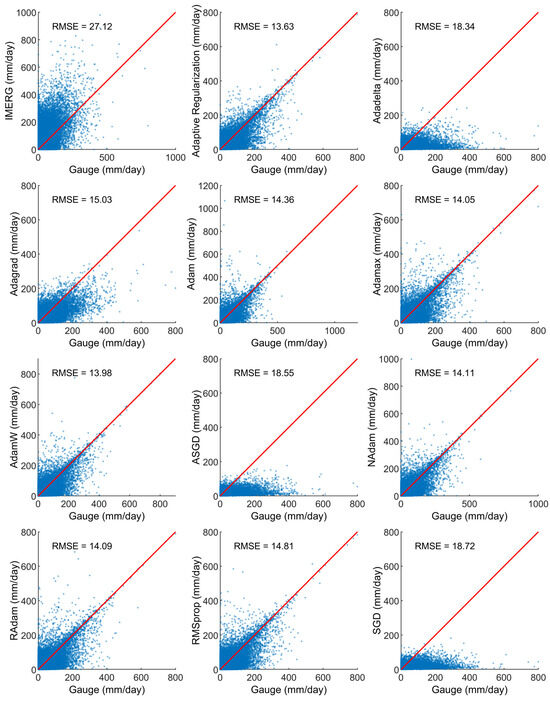
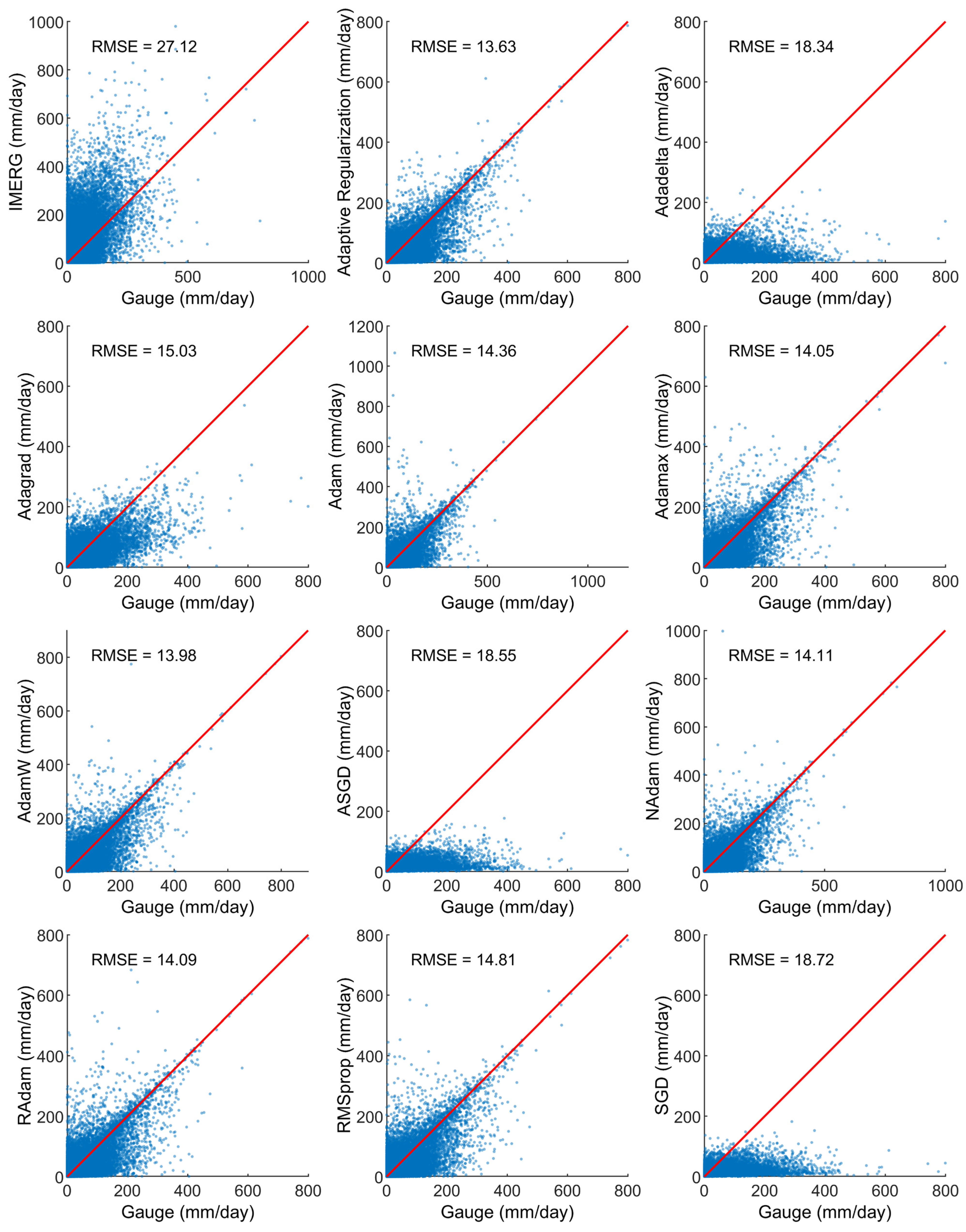
The comparison between daily IMERG estimates and ground-based rain gauge observations (Figure 4) revealed that IMERG systematically overestimated rainfall, particularly during low-intensity events. This bias is consistent with earlier findings that SPE products, while offering excellent spatial coverage, tend to misrepresent localized rainfall due to limitations in sensor resolution and retrieval algorithms. Such discrepancies reinforce the necessity of data-driven post-processing techniques to enhance satellite rainfall accuracy for hydrological applications. Based on the scatter plots, variations in the accuracy of the ML-improved datasets are evident. The ASGD, Adadelta, and SGD datasets exhibit clear underestimation of moderate to high daily precipitation compared with the raw IMERG product, indicating overcorrection during training that led to a reversal from overestimation to underestimation. In contrast, the Adagrad, RMSprop, and Adam-family datasets show improved representation of daily precipitation, with RMSE values ranging from 13.63 to 15.03. Based on this initial comparative analysis, AdamW emerged as the best-performing optimizer within the Adam family, primarily due to its superior regularization capability and efficient optimization. Its decoupled weight decay mechanism is particularly advantageous, as it ensures that regularization is applied consistently and effectively, independent of adaptive learning rate updates. This is crucial for preventing overfitting and improving generalization. Utilizing this identified best optimizer, together with the proposed Adaptive Regularization framework, the Adaptive Regularization dataset demonstrates improved agreement with gauge observations, as indicated by a tighter clustering of points around the 1:1 line and the lowest RMSE value (13.63). The RMSE values for both training and validation datasets under Adaptive Regularization model are 12.60 and 13.35, respectively. The close agreement between validation and test performance, together with slightly lower training error, suggests good generalization with no evidence of significant overfitting. The results further suggest that dynamically adjusting weight decay and the learning rate during the training process plays an important role in enhancing rainfall estimation performance.

Figure 4. Scatter plot for daily rainfall comparison between each optimizer and gauge observations. Red line represents the 1:1 best fit line.

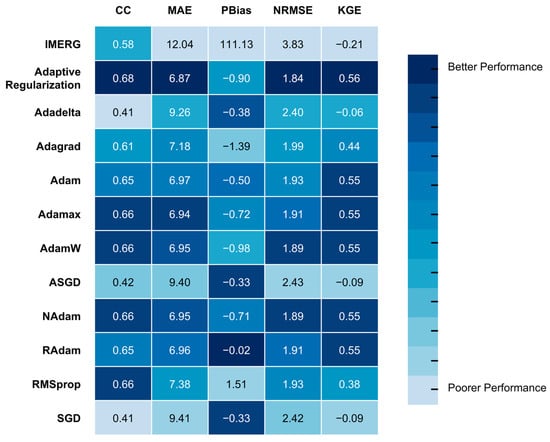
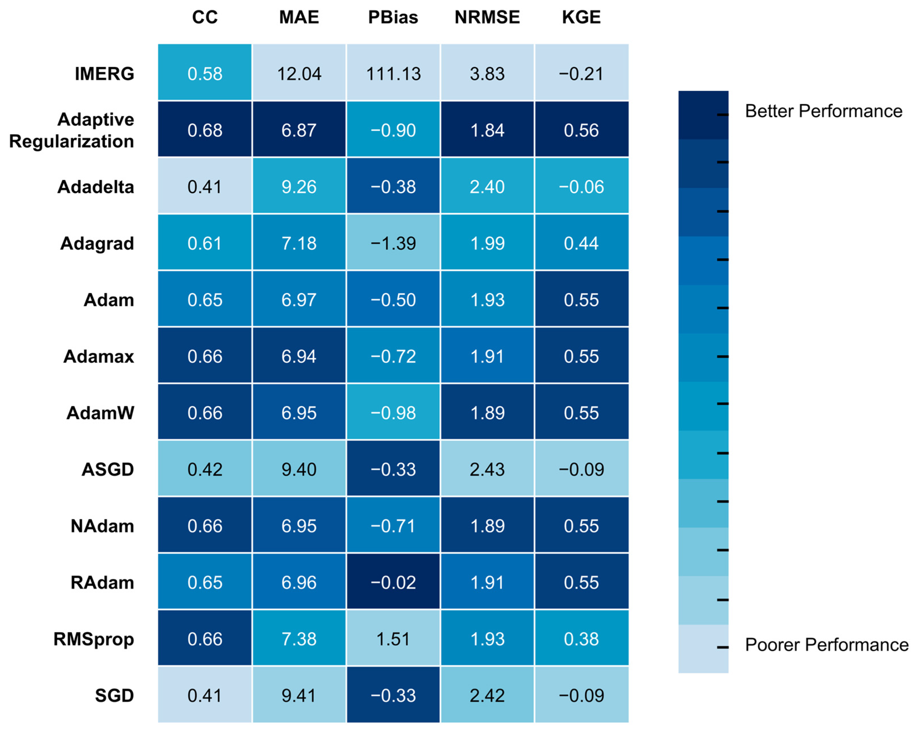
The relative performance of the optimizers in terms of statistical metrics is summarized in Figure 5. Among the ten optimizers evaluated, most exhibit only marginal differences in KGE, with the exception of Adadelta (−0.06), ASGD (−0.09), and SGD (−0.09), which show notably poorer performance. In particular, the Adam variants differ from the original Adam optimizer by less than 1% in CC, MAE, NRMSE, and KGE, indicating that these modifications do not substantially improve precipitation estimation and that performance gains through optimizer selection alone may have reached a plateau. In contrast, the application of Adaptive Regularization yields consistent, albeit modest, improvements over the best-performing Adam variants across all four metrics, including increases of 3% in CC (0.66 to 0.68), 1% in MAE (6.94 to 6.87), 3% in NRMSE (1.89 to 1.84), and 2% in KGE (0.55 to 0.56). Although the ML-improved dataset using Adaptive Regularization shows a slightly poorer PBias compared to the best Adam variant (−0.90 vs. −0.02), the deviation remains small and acceptable, as the PBias error against gauge observations is below 1%. Overall, Adaptive Regularization demonstrates superior performance across four key evaluation metrics (CC, MAE, NRMSE, and KGE) relative to the ten selected optimizers, ranking highest among the tested statistical metrics.

Figure 5. Performance rankings of different optimizers in CC, MAE, PBias, NRMSE and KGE, compared against gauge observations.

4.2. Geospatial Analysis

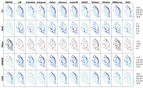
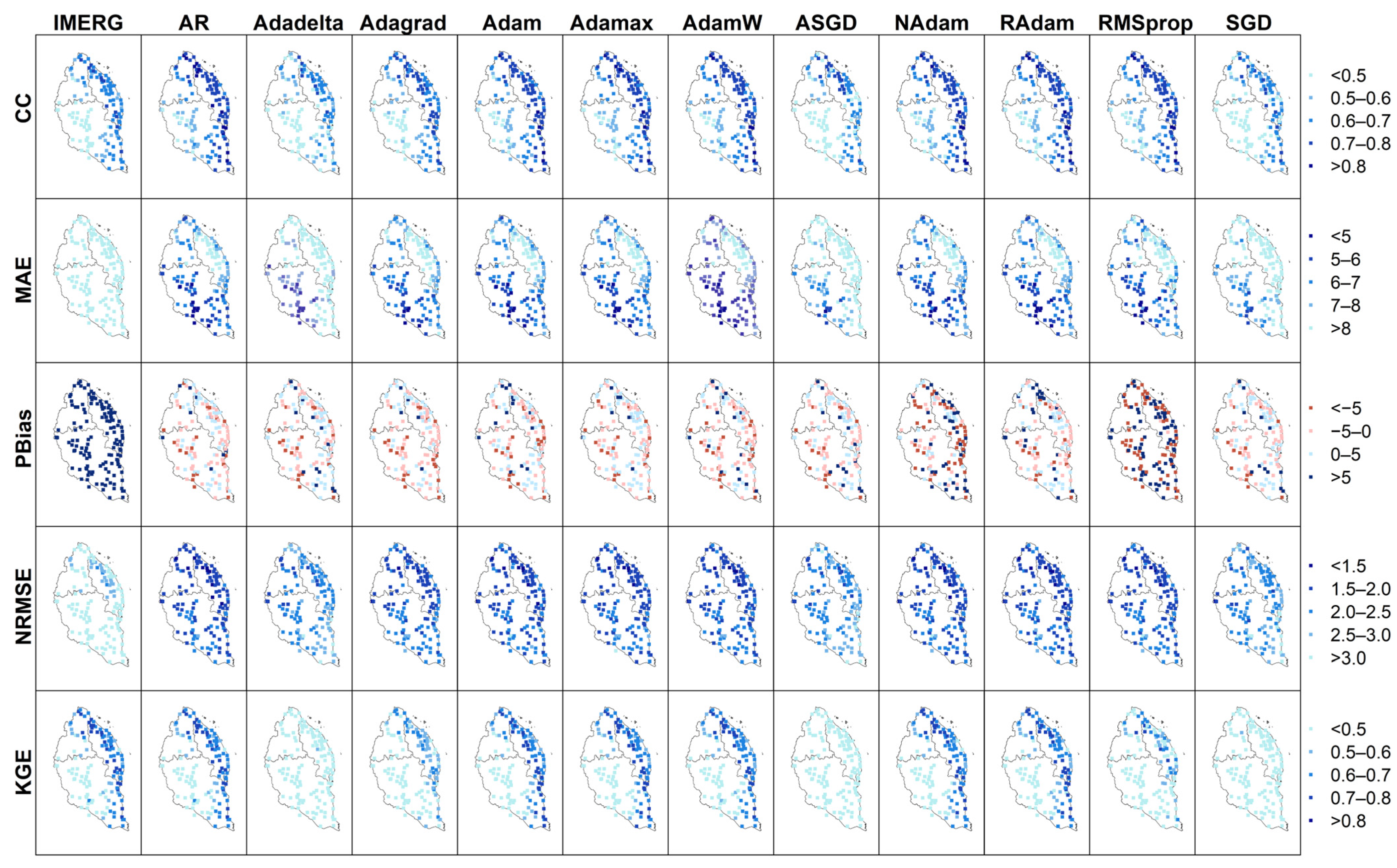
The spatial distribution of model performance (Figure 6) provides insights into how effectively different optimizers capture rainfall variability across Kelantan, Terengganu, and Pahang. The spatial patterns of CC and KGE indicate that higher scores for most datasets are predominantly concentrated along the eastern coastline, whereas lower scores are mainly observed in the western inland regions characterized by more complex terrain (Figure 1). In contrast, the MAE exhibits an opposing spatial pattern, with lower errors distributed over the western inland areas of Pahang and higher errors along the eastern coastal region. For PBias and NRMSE, most products display relatively uniform performance across the study area, with no pronounced localized spatial patterns.

Figure 6. Spatial distribution of CC, MAE, PBias, NRMSE and KGE scores across the study area. AR is the abbreviation for Adaptive Regularization.

A comparison among datasets shows that all model configurations exhibit broadly similar spatial distributions for CC, MAE, and NRMSE. However, NAdam and RMSprop demonstrate notably poorer PBias over larger spatial extents, while Adadelta, ASGD, and SGD show lower KGE values across much of the region compared to the other optimizers. The results indicate largely consistent spatial performance among the evaluated models for most statistical metrics, with the exception of PBias and KGE for a subset of optimizers. The observed region-specific variations in CC, MAE, and KGE further suggest a potential influence of topographic complexity and density of rain gauges on model performance and error characteristics. The reduced gauge density may limit the model’s ability to adequately learn localized precipitation characteristics, thereby affecting its skills in estimating the temporal rainfall dynamics. This highlights a potential limitation of the present study, as model accuracy may be constrained in regions with insufficient observational coverage. Additional data sources can be added in future research to overcome this issue.

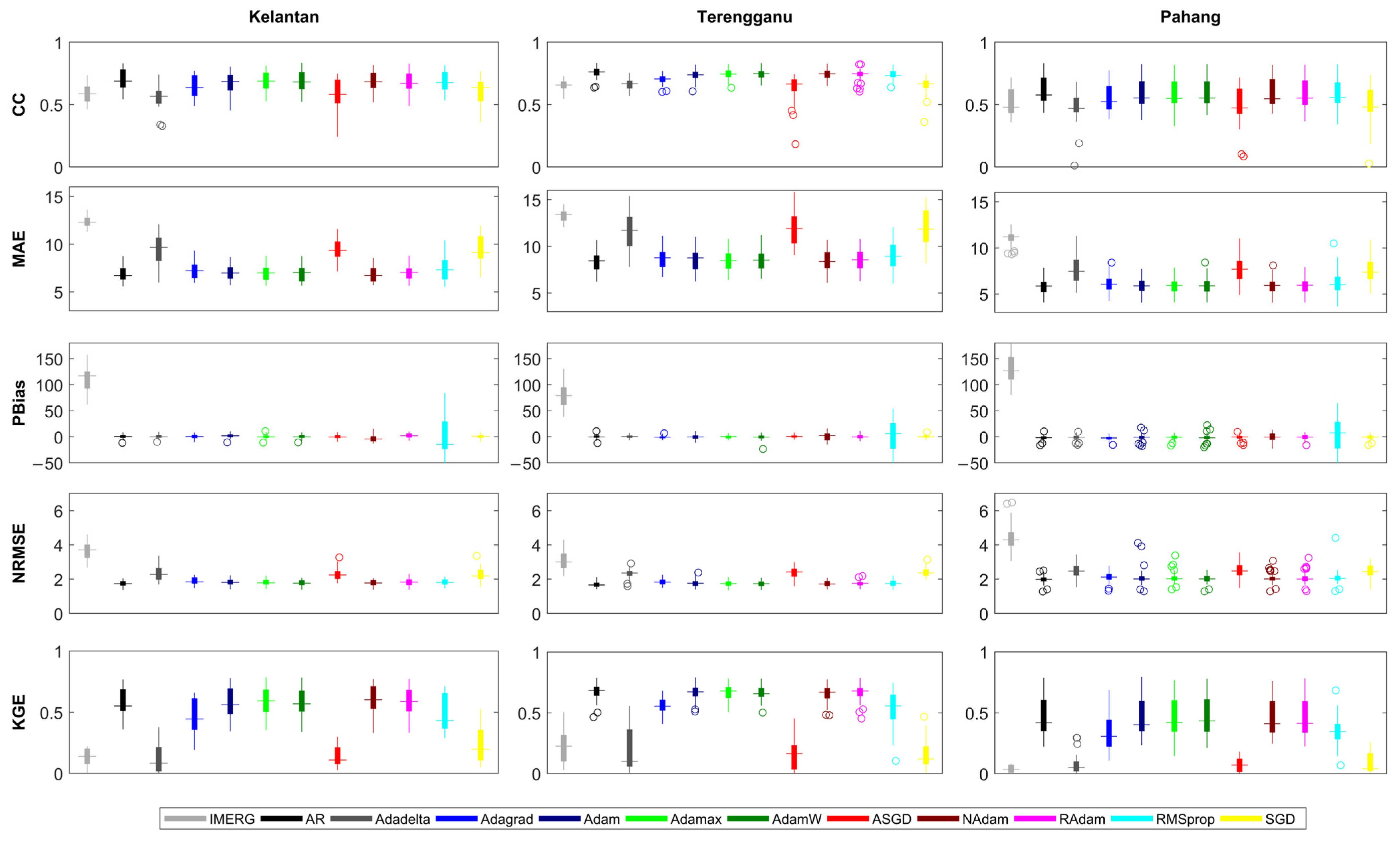
To support regional water resource management, the performance of the model datasets is further evaluated at the regional scale using box-and-whisker plots for the three flood-prone states of Pahang, Kelantan, and Terengganu (Figure 7). The results indicate that all model datasets exhibit broadly similar skill levels across the three states for MAE, PBias, and NRMSE, suggesting limited regional variability for these metrics. In contrast, CC and KGE display more pronounced regional differences. Higher spatial consistency is observed in Terengganu for most datasets, as indicated by narrower interquartile range, while greater variability is evident in Kelantan and Pahang. The median CC and KGE values of most datasets are lowest in Pahang, indicating comparatively poorer model performance in this state, which is consistent with the spatial patterns shown in Figure 6. Among all evaluated approaches, the Adaptive Regularization model demonstrates superior performance, with higher median scores across all statistical metrics in each of the three states. It also exhibits a narrower interquartile range relative to other optimizers, indicating more uniform performance across diverse localities. Such consistency is particularly important for operational water resource management, as spatial heterogeneity in model skill can disproportionately affect flood forecasting and disaster response across regions. The results highlight that the Adaptive Regularization framework not only enhances overall accuracy but also improves spatial consistency, ensuring reliable precipitation estimates across the entire study area rather than concentrating improvements in specific locations.

Figure 7. Box plot of performance metrics for regional comparison. AR is the abbreviation for Adaptive Regularization.

4.3. Seasonal Variability in Model Performance

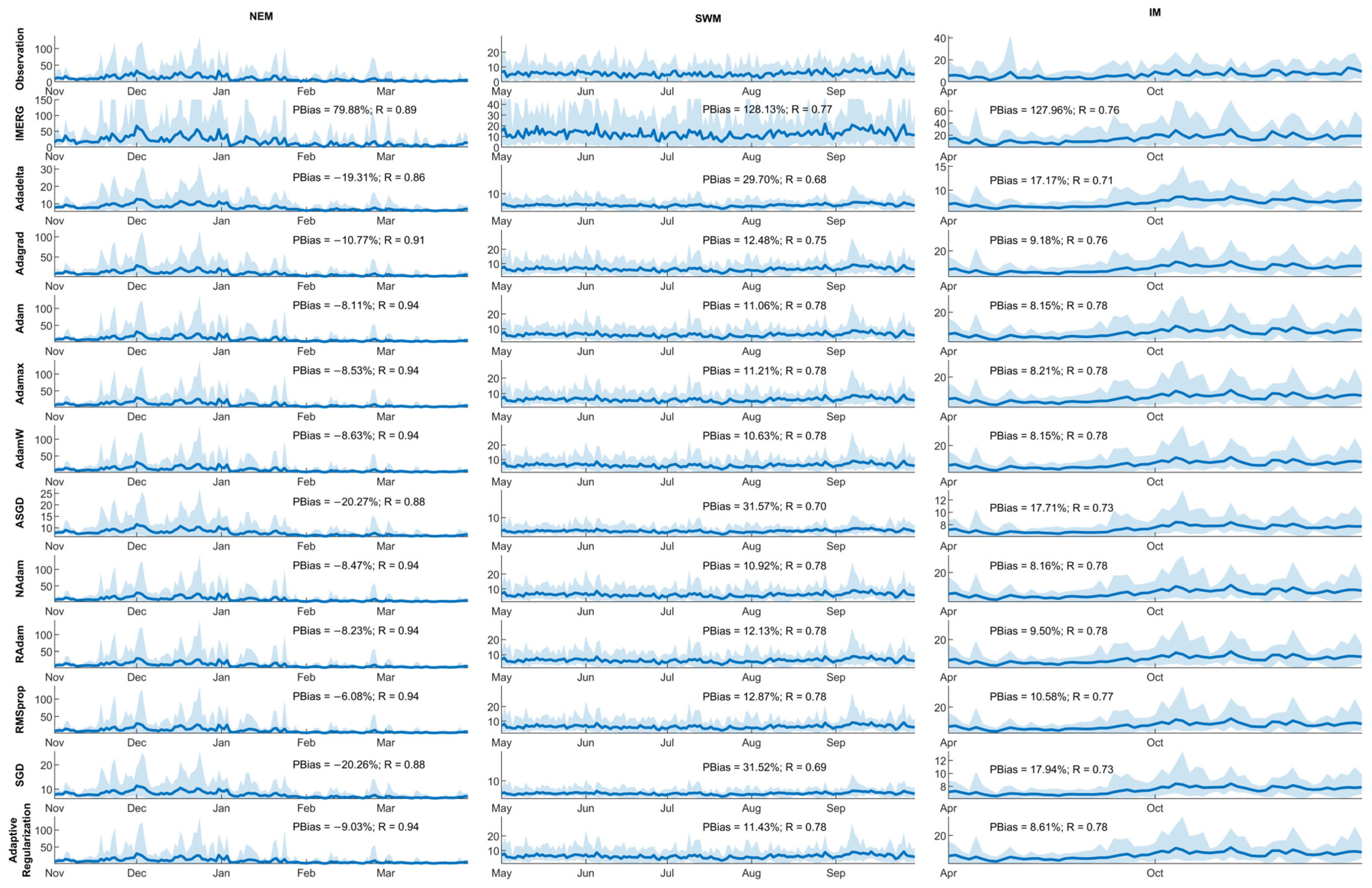
The tropical monsoon cycle introduces additional complexity to rainfall estimation over the ECPM–PKT region. To assess the ability of the models to capture interannual monsoon variability from 2011 to 2020, domain-averaged time series were segregated by monsoon season. This approach facilitates clearer visualization of seasonal rainfall peaks for each monsoon period (Figure 8). The time series clearly indicate higher seasonal rainfall during the NEM season compared with the SWM and IM seasons. This distinction is particularly important for the ECPM–PKT region, where intense NEM rainfall frequently triggers severe flooding. In terms of seasonal model performance, all datasets show stronger correlations with gauge observations during the NEM season (R > 0.8) than during the SWM (R = 0.68–0.78) and IM (R = 0.71–0.78) seasons. Similarly, PBias values are smallest during the IM (8.15–17.94%) season, followed by the NEM (−20.27% to −6.08%) and SWM (10.63–31.57%) seasons, indicating closer agreement with observations during the wet monsoon period. Notably, all models tend to underestimate rainfall during the NEM season while overestimating it during the IM and SWM seasons. Based on the range of variability, these models are generally able to capture temporal variations but fail to accurately represent the magnitude of variability. These results suggest that, although the models reproduce temporal patterns reasonably well, they struggle to accurately represent wet and dry extremes across different monsoon regimes.

Figure 8. Comparison of domain average time series during the NEM, SWM and IM seasons. Solid blue lines represent the multi-year mean values, while shaded areas represent range of variability.

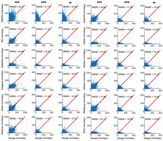
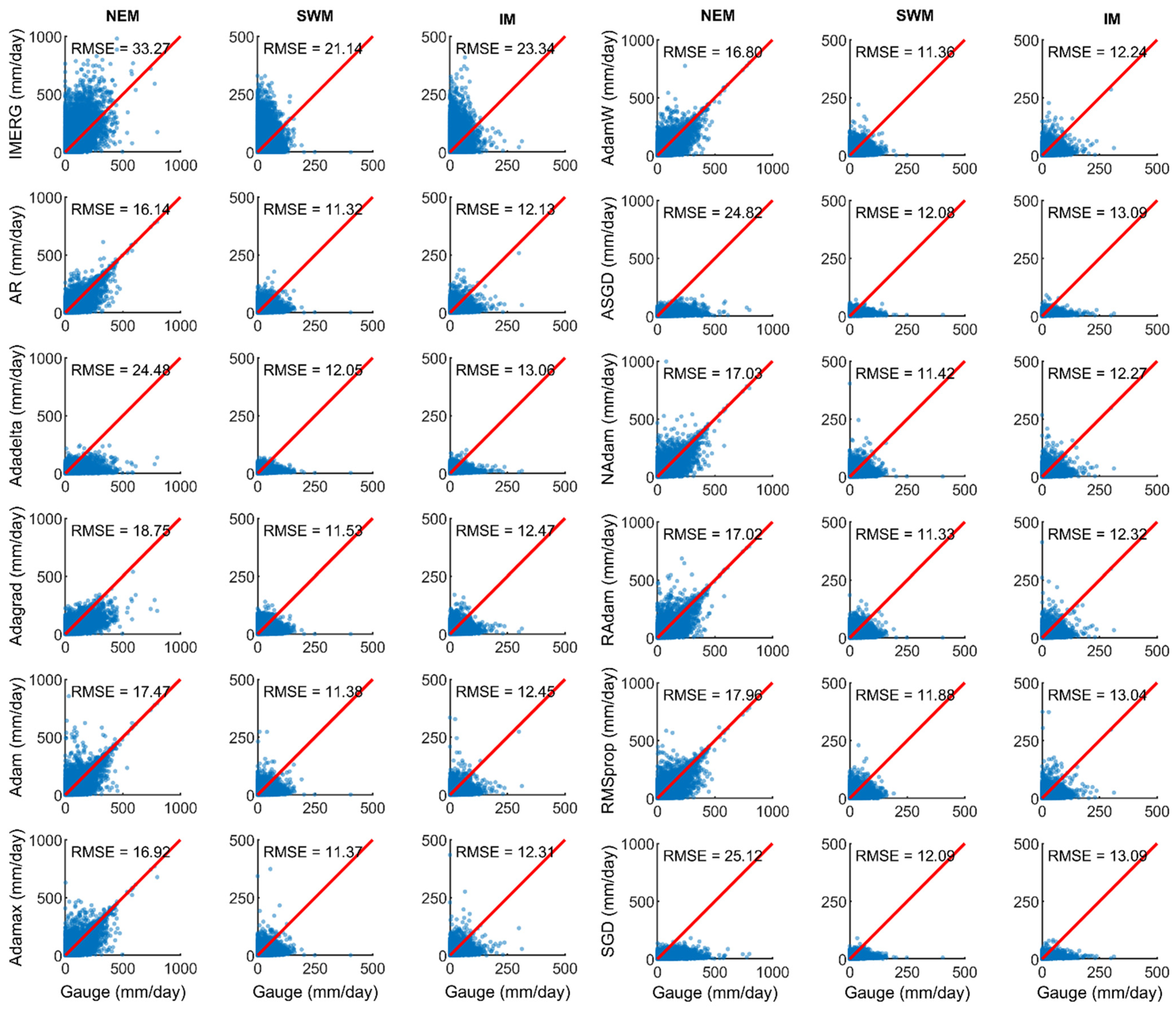
The scatter plots of seasonal rainfall indicate that the Adaptive Regularization approach consistently outperforms other models across all three monsoon seasons, with RMSE values of 16.14, 11.32, and 12.13 for the NEM, SWM, and IM seasons, respectively (Figure 9). These seasonal evaluations demonstrate that the Adaptive Regularization framework is robust under both wet and dry conditions, highlighting its suitability for year-round operational forecasting and climate monitoring. Among the tested optimizers, the Adam family generally exhibits superior performance compared to other optimizers, including Adadelta, RMSprop, and SGD variants.

Figure 9. Scatter plot for daily rainfall comparison during the NEM, SWM and IM seasons. Red line represents the 1:1 best fit line.

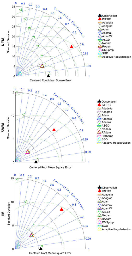
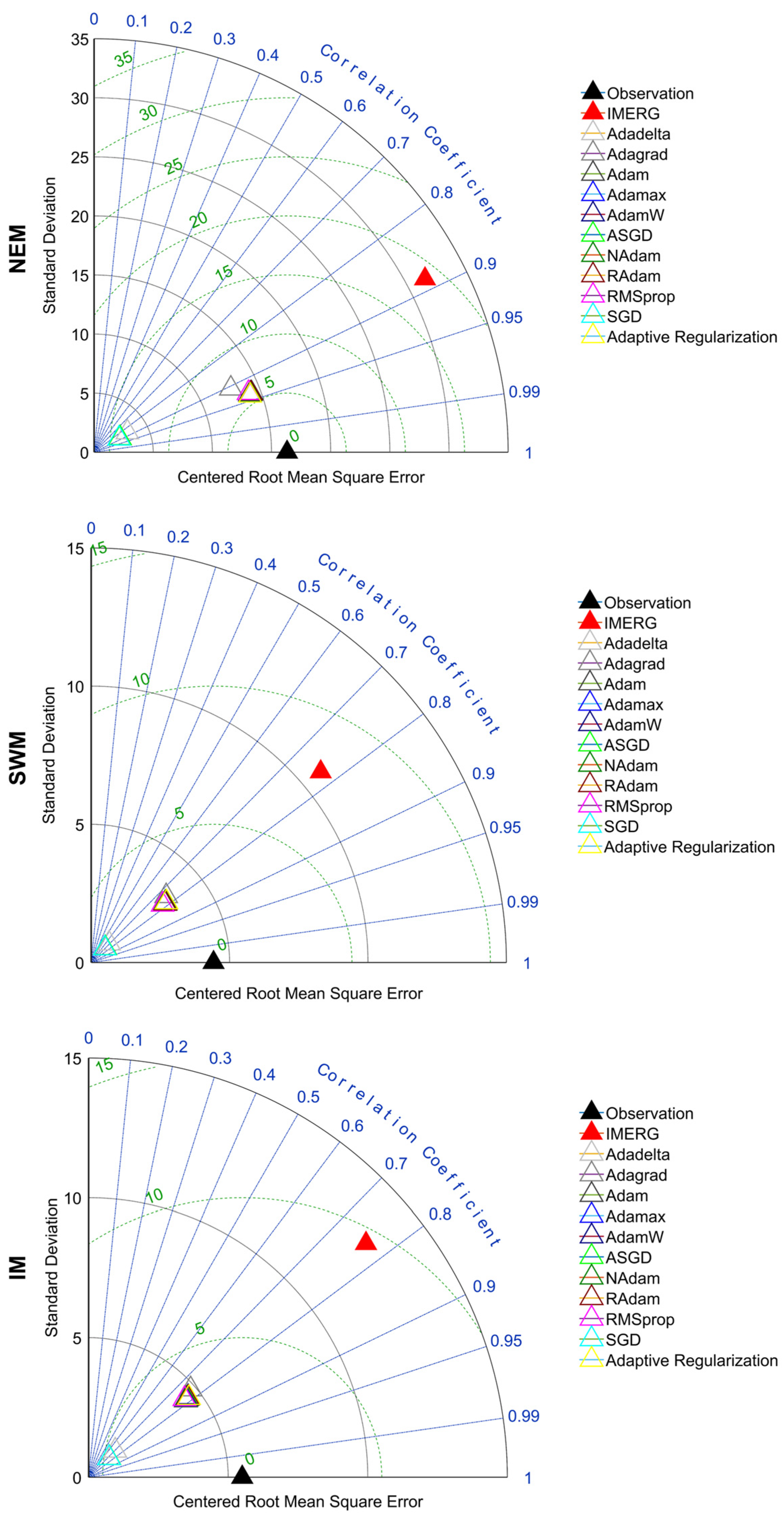
The Taylor diagrams for different monsoon seasons indicate that the NEM season exhibits the highest standard deviation (16.3), followed by the IM (5.5) and SWM (4.4) seasons (Figure 10). The larger standard deviation during the NEM season reflects greater rainfall variability, which is consistent with the seasonal time series shown in Figure 8. Nevertheless, all models tend to underestimate the observed rainfall variability relative to gauge observations across all monsoon seasons. Among the evaluated datasets, the Adaptive Regularization approach and the Adam variants provide a closer representation of the observed standard deviation, correlation coefficient, and centered root mean square error compared to the other optimizers.

Figure 10. Taylor diagrams for the models during the NEM, SWM and IM seasons.

4.4. Contribution of Adaptive Regularization

The most significant advancement of this study lies in the integration of Adaptive Regularization with the LSTM–AdamW framework. Unlike static regularization methods, which apply fixed penalties, the adaptive approach dynamically adjusts the learning rate and weight decay during training in response to validation loss trends and explicit overfitting signals. This proactive strategy allowed the model to continuously refine its balance between bias and variance, improving both convergence and generalization.

Quantitatively, the adaptive framework achieved an MAE of 6.87, CC of 0.68, NRMSE of 1.84, and KGE of 0.56, representing a 1–3% improvement over the baseline AdamW optimizer. Although these numerical gains may appear modest, they should be interpreted within the context of a performance plateau, where widely used optimizers such as the Adam family tend to converge to similar solutions with marginal differences (often <1%). In such a setting, further improvements become increasingly difficult to achieve, and even small gains are indicative of meaningful methodological advancement rather than random variation.

Importantly, the improvements observed are not limited to aggregated performance metrics but are consistently reflected across spatial and temporal dimensions. The adaptive framework demonstrates enhanced spatial consistency, particularly in regions with complex terrain, as well as reduced seasonal bias across different monsoon regimes. These improvements indicate that the model is better able to capture the underlying variability of precipitation processes, including both wet and dry conditions, which are critical for hydrological applications. From a practical perspective, even small reductions in error can lead to more reliable precipitation estimates, especially when propagated through downstream applications such as flood forecasting, water resource management, and risk assessment, where errors may accumulate and amplify.

Furthermore, the Adaptive Regularization mechanism contributes to improved training stability by preventing both overfitting and underfitting through continuous feedback from validation performance. This dynamic adjustment allows the model to respond to changing learning conditions during training, which is particularly important for precipitation data characterized by strong non-linearity, intermittency, and spatiotemporal heterogeneity. As such, the improvements achieved are not merely incremental in magnitude but reflect a more robust and stable learning process.

Overall, the proposed adaptive framework demonstrates that incorporating dynamic, feedback-driven hyperparameter adjustment can overcome limitations associated with static optimization strategies and unlock additional performance gains, even in well-optimized settings. This approach not only advances methodological development in deep learning for hydrology but also delivers tangible benefits for operational flood forecasting and water resource planning in flood-prone regions such as ECPM.

5. Conclusions

Satellite-derived precipitation estimates often exhibit systematic biases in regions with complex terrain, whereas rain gauge observations provide more accurate measurements but are spatially sparse. Although ML approaches have shown promise in improving SPE, they are subject to limitations such as overfitting, which may hinder their ability to realistically represent spatially and temporally varying atmospheric conditions. To address this challenge, this study proposes a scalable framework for global precipitation mapping based on an Adaptive Regularization approach within an LSTM–AdamW deep learning architecture. The proposed method is evaluated against ten commonly used optimizers aimed at enhancing SPE skill. All models were trained using IMERG precipitation data and observations from 131 operational rain gauge stations across the ECPM-PKT region for the period 2011–2020.

Our findings indicate that the Adaptive Regularization model achieved an MAE of 6.87, a CC of 0.68, an NRMSE of 1.84, and a KGE of 0.56, outperforming the other optimizers by 1–3%, but exhibiting poorer performance in terms of PBias compared to other Adam variants. These improvements are noteworthy given that the Adam variants exhibited only marginal gains (<1%) relative to the original Adam optimizer, suggesting a performance plateau in conventional optimization approaches. In addition to enhanced overall accuracy, the Adaptive Regularization model improved the spatial consistency of precipitation estimates across the three states in the study area. Temporally, it also consistently outperformed the other models across all three monsoon seasons in terms of both numerical metrics and variability representation, indicating robust performance under both wet and dry conditions. Overall, the proposed Adaptive Regularization framework effectively leverages the AdamW optimizer to achieve state-of-the-art performance, surpassing existing optimizers in providing meaningful advances in satellite-based precipitation estimation. However, limitations related to lower performance in complex terrain and areas with sparse rain gauge coverage have been addressed in the discussion, underscoring the need for improved observational networks or supplementary data sources to enhance model reliability in topographically complex regions.

Future studies could incorporate additional modalities like soil data monitoring, explore transfer learning for low-data environments, or evaluate real-time deployment for data forecasting. Ultimately, this deep learning model represents a step forward in more reliable, AI-driven Earth observation, paving the way for resilient environment management in changing climate. The recommendation for further studies is to implement Adaptive Regularization with combination of other deep learning models, like Convolutional Neural Network (CNN).

Appendix A.1

Table A1. Summary of optimizers.

Optimizers	Description
Stochastic Gradient Descent (SGD)	Stochastic Gradient Descent (SGD) is the most basic and widely used optimizer in PyTorch. SGD updates the weights of the neural network by subtracting the product of the learning rate and the gradient of the loss function with respect to the weights. Its operation is governed by $w_{t+1}=w_t-\eta \nabla L\left(w_t\right),$ where η is the learning rate and ∇L is the gradient. The learning rate determines the step size at which the optimizer updates the weights [53].
ADAM	ADAM is an adaptive learning rate optimizer that can adapt the learning rate based on the gradient of the loss function. Adam combines momentum and adaptive learning rates by maintaining first (mt) and second (vt) moment estimates of the gradients, updating weights as $w_{t+1}=w_t-\eta {\displaystyle \frac{{\widehat{m}}_t}{\sqrt{{\widehat{v}}_t}+ϵ}}.$ Adam is widely used in deep learning algorithms because of its ability to converge quickly. Adam requires less tuning of its hyperparameters [27].
Adagrad	Adagrad is an adaptive learning rate optimizer that adapts the learning rate based on the frequency of updates to each weight. Adagrad adjusts the learning rate for each parameter individually based on cumulative squared gradients ${\eta }_t={\displaystyle \frac{\eta }{\sqrt{G_t+ϵ}}}\odot g_t,$ making it suitable for sparse gradients [26].
Adadelta	Adadelta is an adaptive learning rate optimizer that is an extension of Adagrad. Adadelta uses an exponentially decaying average of squared gradients $(∆w_t=-{\displaystyle \frac{RMS{\left[∆w\right]}_{t-1}}{RMS{\left[g\right]}_t}}{g}_t$) to scale updates, avoiding continual learning rate decay. Adadelta is designed to converge faster than Adagrad and is suitable for large-scale problems [31].
RMSprop	RMSprop is an adaptive learning rate optimizer that uses a moving average of the squared gradients to adjust the learning rate. Similar to Adadelta, RMSprop maintains a moving average of squared gradients to normalize updates: $∆w_t=-\eta {\displaystyle \frac{g_t}{\sqrt{E{\left[g^2\right]}_t}+ϵ}}.$ RMSprop is widely used in deep learning algorithms because of its ability to converge quickly [30].
Adamax	Adamax is a variant of Adam optimizer that adaptively adjust the learning rates to individual parameters. As compared to Adam which computes the first and second moments of the gradients, Adamax only calculates the uncentered variance. It uses the infinity norm for scaling $w_{t+1}=w_t-{\displaystyle \frac{\eta }{u_t+ϵ}}\times m_t,$ where ut is the maximum of past gradients’ absolute values. This gives Adamax better performance as its simplification results in more memory-efficient algorithm [27].
AdamW	AdamW is another variant of Adam optimizer that introduces weight decay directly into the update step, separating regularization from adaptive learning. Weight decay is used to penalize large weights in the network by adding a term proportional to the square of the weights of the loss function: $w_{t+1}=w_t-\eta ({\displaystyle \frac{{\widehat{m}}_t}{\sqrt{{\widehat{v}}_t}+ϵ}}+{\lambda w}_t)$ This helps prevent overfitting and encourages the model to learn simpler and more generalization representations [32].
Average Stochastic Gradient Descent (ASGD)	Average Stochastic Gradient Descent (ASGD) is a variant of SGD optimizer that incorporates the idea of averaging gradients over time to improve convergence: ${\overline{w}}_t={\displaystyle \frac{1}{t}}\sum _{i=1}^t{w}_i.$ The gradients are averaged over multiple mini-batches or iterations to help smoothing out the noisy updates in SGD which leads to more stable convergence and potentially better generalization [54].
NAdam	NAdam stands for Nesterov-accelerated Adaptive Moment Estimation, is an extension of Adam optimizer that adjusts the momentum term in such a way that it evaluates gradient at the lookahead position: $w_{t+1}=w_t-\eta {\displaystyle \frac{{\beta }_1{\widehat{m}}_{t+1}+(1-{\beta }_1)g_t}{\sqrt{{\widehat{v}}_t}+ϵ}}.$ It helps accelerate convergence, especially in the presence of high curvature gradients [55].
RAdam	RAdam, abbreviation for “Rectified Adam”, is an optimization algorithm proposed as an improvement over the original Adam optimizer. It addresses some of the shortcomings of Adam, particularly in the scenarios where the adaptive learning rate might not be well-initialized. Radam dynamically adjusts the learning rate to stabilize early training by computing variance rectification: ${\eta }_t=\eta \times r_t,$ where rt adjusts the step size based on the variance of past gradients [56].

Table A1. Summary of optimizers.

Optimizers	Description
Stochastic Gradient Descent (SGD)	Stochastic Gradient Descent (SGD) is the most basic and widely used optimizer in PyTorch. SGD updates the weights of the neural network by subtracting the product of the learning rate and the gradient of the loss function with respect to the weights. Its operation is governed by $w_{t+1}=w_t-\eta \nabla L\left(w_t\right),$ where η is the learning rate and ∇L is the gradient. The learning rate determines the step size at which the optimizer updates the weights [53].
ADAM	ADAM is an adaptive learning rate optimizer that can adapt the learning rate based on the gradient of the loss function. Adam combines momentum and adaptive learning rates by maintaining first (mt) and second (vt) moment estimates of the gradients, updating weights as $w_{t+1}=w_t-\eta {\displaystyle \frac{{\widehat{m}}_t}{\sqrt{{\widehat{v}}_t}+ϵ}}.$ Adam is widely used in deep learning algorithms because of its ability to converge quickly. Adam requires less tuning of its hyperparameters [27].
Adagrad	Adagrad is an adaptive learning rate optimizer that adapts the learning rate based on the frequency of updates to each weight. Adagrad adjusts the learning rate for each parameter individually based on cumulative squared gradients ${\eta }_t={\displaystyle \frac{\eta }{\sqrt{G_t+ϵ}}}\odot g_t,$ making it suitable for sparse gradients [26].
Adadelta	Adadelta is an adaptive learning rate optimizer that is an extension of Adagrad. Adadelta uses an exponentially decaying average of squared gradients $(∆w_t=-{\displaystyle \frac{RMS{\left[∆w\right]}_{t-1}}{RMS{\left[g\right]}_t}}{g}_t$) to scale updates, avoiding continual learning rate decay. Adadelta is designed to converge faster than Adagrad and is suitable for large-scale problems [31].
RMSprop	RMSprop is an adaptive learning rate optimizer that uses a moving average of the squared gradients to adjust the learning rate. Similar to Adadelta, RMSprop maintains a moving average of squared gradients to normalize updates: $∆w_t=-\eta {\displaystyle \frac{g_t}{\sqrt{E{\left[g^2\right]}_t}+ϵ}}.$ RMSprop is widely used in deep learning algorithms because of its ability to converge quickly [30].
Adamax	Adamax is a variant of Adam optimizer that adaptively adjust the learning rates to individual parameters. As compared to Adam which computes the first and second moments of the gradients, Adamax only calculates the uncentered variance. It uses the infinity norm for scaling $w_{t+1}=w_t-{\displaystyle \frac{\eta }{u_t+ϵ}}\times m_t,$ where ut is the maximum of past gradients’ absolute values. This gives Adamax better performance as its simplification results in more memory-efficient algorithm [27].
AdamW	AdamW is another variant of Adam optimizer that introduces weight decay directly into the update step, separating regularization from adaptive learning. Weight decay is used to penalize large weights in the network by adding a term proportional to the square of the weights of the loss function: $w_{t+1}=w_t-\eta ({\displaystyle \frac{{\widehat{m}}_t}{\sqrt{{\widehat{v}}_t}+ϵ}}+{\lambda w}_t)$ This helps prevent overfitting and encourages the model to learn simpler and more generalization representations [32].
Average Stochastic Gradient Descent (ASGD)	Average Stochastic Gradient Descent (ASGD) is a variant of SGD optimizer that incorporates the idea of averaging gradients over time to improve convergence: ${\overline{w}}_t={\displaystyle \frac{1}{t}}\sum _{i=1}^t{w}_i.$ The gradients are averaged over multiple mini-batches or iterations to help smoothing out the noisy updates in SGD which leads to more stable convergence and potentially better generalization [54].
NAdam	NAdam stands for Nesterov-accelerated Adaptive Moment Estimation, is an extension of Adam optimizer that adjusts the momentum term in such a way that it evaluates gradient at the lookahead position: $w_{t+1}=w_t-\eta {\displaystyle \frac{{\beta }_1{\widehat{m}}_{t+1}+(1-{\beta }_1)g_t}{\sqrt{{\widehat{v}}_t}+ϵ}}.$ It helps accelerate convergence, especially in the presence of high curvature gradients [55].
RAdam	RAdam, abbreviation for “Rectified Adam”, is an optimization algorithm proposed as an improvement over the original Adam optimizer. It addresses some of the shortcomings of Adam, particularly in the scenarios where the adaptive learning rate might not be well-initialized. Radam dynamically adjusts the learning rate to stabilize early training by computing variance rectification: ${\eta }_t=\eta \times r_t,$ where rt adjusts the step size based on the variance of past gradients [56].

Appendix A.2

Table A2. Root mean squared error (RMSE) of each optimizer during training and validation, compared against gauge observations. The RMSE of the raw IMERG dataset, without ML-based improvement, was 27.12.

Optimizers	Training	Validation
Adaptive Regularization	12.60	13.35
Adadelta	16.64	15.53
Adagrad	14.73	15.03
Adam	12.83	14.60
Adamax	12.78	13.97
AdamW	12.73	13.67
ASGD	17.30	16.01
NAdam	12.81	14.86
Radam	12.76	14.07
RMSprop	13.95	14.51
SGD	17.53	16.24

Table A2. Root mean squared error (RMSE) of each optimizer during training and validation, compared against gauge observations. The RMSE of the raw IMERG dataset, without ML-based improvement, was 27.12.

Optimizers	Training	Validation
Adaptive Regularization	12.60	13.35
Adadelta	16.64	15.53
Adagrad	14.73	15.03
Adam	12.83	14.60
Adamax	12.78	13.97
AdamW	12.73	13.67
ASGD	17.30	16.01
NAdam	12.81	14.86
Radam	12.76	14.07
RMSprop	13.95	14.51
SGD	17.53	16.24

References

- Beck, H.E.; Pan, M.; Roy, T.; Weedon, G.P.; Pappenberger, F.; van Dijk, A.I.J.M.; Huffman, G.J.; Adler, R.F.; Wood, E.F. Daily evaluation of 26 precipitation datasets using Stage-IV gauge-radar data for the CONUS. Hydrol. Earth Syst. Sci. 2019, 23, 207–224. [Google Scholar] [CrossRef] [Scilit]
- Kidd, C.; Huffman, G. Global precipitation measurement. Meteorol. Appl. 2011, 18, 334–353. [Google Scholar] [CrossRef] [Scilit]
- Ashouri, H.; Hsu, K.-L.; Sorooshian, S.; Braithwaite, D.K.; Knapp, K.R.; Cecil, L.D.; Nelson, B.R.; Prat, O.P. PERSIANN-CDR: Daily precipitation climate data record from multisatellite observations for hydrological and climate studies. Bull. Am. Meterol. Soc. 2015, 96, 69–83. [Google Scholar] [CrossRef] [Scilit]
- Beck, H.E.; Wood, E.F.; Pan, M.; Fisher, C.K.; Miralles, D.G.; van Dijk, A.I.J.M.; McVicar, T.R.; Adler, R.F. MSWEP V2 global 3-hourly 0.1° precipitation: Methodology and quantitative assessment. Bull. Am. Meterol. Soc. 2019, 100, 473–500. [Google Scholar] [CrossRef] [Scilit]
- Funk, C.; Peterson, P.; Landsfeld, M.; Pedreros, D.; Verdin, J.; Shukla, S.; Husak, G.; Rowland, J.; Harrison, L.; Hoell, A.; et al. The climate hazards infrared precipitation with stations—A new environmental record for monitoring extremes. Sci. Data 2015, 2, 150066. [Google Scholar] [CrossRef] [Scilit]
- Hersbach, H.; Bell, B.; Berrisford, P.; Hirahara, S.; Horányi, A.; Muñoz-Sabater, J.; Nicolas, J.; Peubey, C.; Radu, R.; Schepers, D.; et al. The ERA5 global reanalysis. Q. J. R. Meteorol. Soc. 2020, 146, 1999–2049. [Google Scholar] [CrossRef] [Scilit]
- Hou, A.Y.; Kakar, R.K.; Neeck, S.; Azarbarzin, A.A.; Kummerow, C.D.; Kojima, M.; Oki, R.; Nakamura, K.; Iguchi, T. The global precipitation measurement mission. Bull. Am. Meterol. Soc. 2014, 95, 701–722. [Google Scholar] [CrossRef] [Scilit]
- Xie, P.; Joyce, R.; Wu, S.; Yoo, S.-H.; Yarosh, Y.; Sun, F.; Lin, R. Reprocessed, bias-corrected CMORPH global high-resolution precipitation estimates from 1998. J. Hydrometeorol. 2017, 18, 1617–1641. [Google Scholar] [CrossRef] [Scilit]
- Kaprom, C.; Williams, J.A.; Mehrotra, R.; Ophaphaibun, C.; Sriwongsitanon, N. A comprehensive evaluation of the accuracy of satellite-based precipitation estimates over Thailand. J. Hydrol. Reg. Stud. 2025, 59, 102380. [Google Scholar] [CrossRef] [Scilit]
- Kumar, S.; Amarnath, G.; Ghosh, S.; Park, E.; Baghel, T.; Wang, J.; Pramanik, M.; Belbase, D. Assessing the performance of the satellite-based precipitation products (SPP) in the data-sparse Himalayan terrain. Remote Sens. 2022, 14, 4810. [Google Scholar] [CrossRef] [Scilit]
- Mei, Y.; Anagnostou, E.N.; Nikolopoulos, E.I.; Borga, M. Error analysis of satellite precipitation products in mountainous basins. J. Hydrometeorol. 2014, 15, 1778–1793. [Google Scholar] [CrossRef] [Scilit]
- Dhawan, P.; Dalla Torre, D.; Niazkar, M.; Kaffas, K.; Larcher, M.; Righetti, M.; Menapace, A. A comprehensive comparison of bias correction methods in climate model simulations: Application on ERA5-Land across different temporal resolutions. Heliyon 2024, 10, e40352. [Google Scholar] [CrossRef] [Scilit] [PubMed]
- Elsebaie, I.H.; Kawara, A.Q.; Alharbi, R.; Alnahit, A.O. Bias correction methods applied to satellite rainfall products over the western part of Saudi Arabia. Atmosphere 2025, 16, 772. [Google Scholar] [CrossRef] [Scilit]
- Soo, E.Z.X.; Wan Jaafar, W.Z.; Lai, S.H.; Othman, F.; Elshafie, A.; Islam, T.; Srivastava, P.; Hadi, H.S.O. Evaluation of bias-adjusted satellite precipitation estimations for extreme flood events in Langat river basin, Malaysia. Hydrol. Res. 2019, 51, 105–126. [Google Scholar] [CrossRef] [Scilit]
- Teutschbein, C.; Seibert, J. Bias correction of regional climate model simulations for hydrological climate-change impact studies: Review and evaluation of different methods. J. Hydrol. 2012, 456–457, 12–29. [Google Scholar] [CrossRef] [Scilit]
- Themeßl, M.J.; Gobiet, A.; Heinrich, G. Empirical-statistical downscaling and error correction of regional climate models and its impact on the climate change signal. Clim. Change 2012, 112, 449–468. [Google Scholar] [CrossRef] [Scilit]
- Rajulapati, C.R.; Papalexiou, S.M. Precipitation bias correction: A novel semi-parametric quantile mapping method. Earth Space Sci. 2023, 10, e2023EA002823. [Google Scholar] [CrossRef] [Scilit]
- Chen, C.; Hao, J.; Yang, S.; Li, Y. Blending daily satellite precipitation product and rain gauges using stacking ensemble machine learning with the consideration of spatial heterogeneity. J. Hydrol. 2025, 658, 133223. [Google Scholar] [CrossRef] [Scilit]
- Sodunke, M.A.; Ojo, J.S.; Lawal, Y.B.; Ojo, O.L.; Owolabi, G.A.; Olateju, A.I. Application of machine learning models for rainfall prediction and estimation of rain-induced attenuation for satellite communication in a tropical region. J. Atmos. Sol. Terr. Phys. 2025, 268, 106443. [Google Scholar] [CrossRef] [Scilit]
- Kaur, M.; Mohta, A. A review of deep learning with recurrent neural network. In Proceedings of the International Conference on Smart Systems and Inventive Technology (ICSSIT), Tirunelveli, India, 27–29 November 2019; pp. 460–465. [Google Scholar]
- Akbari Asanjan, A.; Yang, T.; Hsu, K.; Sorooshian, S.; Lin, J.; Peng, Q. Short-term precipitation forecast based on the PERSIANN system and LSTM recurrent neural networks. J. Geophys. Res. Atmos. 2018, 123, 12543–12563. [Google Scholar] [CrossRef] [Scilit]
- Dehghani, A.; Moazam, H.M.Z.H.; Mortazavizadeh, F.; Ranjbar, V.; Mirzaei, M.; Mortezavi, S.; Ng, J.L.; Dehghani, A. Comparative evaluation of LSTM, CNN, and ConvLSTM for hourly short-term streamflow forecasting using deep learning approaches. Ecol. Inform. 2023, 75, 102119. [Google Scholar] [CrossRef] [Scilit]
- Miao, Q.; Pan, B.; Wang, H.; Hsu, K.; Sorooshian, S. Improving monsoon precipitation prediction using combined convolutional and Long Short Term Memory neural network. Water 2019, 11, 977. [Google Scholar] [CrossRef] [Scilit]
- Ouma, Y.O.; Cheruyot, R.; Wachera, A.N. Rainfall and runoff time-series trend analysis using LSTM recurrent neural network and wavelet neural network with satellite-based meteorological data: Case study of Nzoia hydrologic basin. Complex Intell. Syst. 2021, 8, 213–236. [Google Scholar] [CrossRef] [Scilit]
- Amari, S.-i. Backpropagation and stochastic gradient descent method. Neurocomputing 1993, 5, 185–196. [Google Scholar] [CrossRef] [Scilit]
- Duchi, J.; Hazan, E.; Singer, Y. Adaptive subgradient methods for online learning and stochastic optimization. J. Mach. Learn. Res. 2011, 12, 2121–2159. [Google Scholar]
- Kingma, D.P.; Ba, J. Adam: A method for stochastic optimization. arXiv 2014. [Google Scholar] [CrossRef] [Scilit]
- Robbins, H.; Monro, S. A stochastic approximation method. Ann. Math. Stat. 1951, 22, 400–407. [Google Scholar] [CrossRef] [Scilit]
- Sharma, O. Deep challenges associated with deep learning. In Proceedings of the International Conference on Machine Learning, Big Data, Cloud and Parallel Computing (COMITCon), Faridabad, India, 14–16 February 2019; pp. 72–75. [Google Scholar]
- Tieleman, T.; Hinton, G. Lecture 6.5-Rmsprop: Divide the Gradient by a Running Average of Its Recent Magnitude. Available online: https://www.cs.toronto.edu/~tijmen/csc321/slides/lecture_slides_lec6.pdf (accessed on 1 June 2025).
- Zeiler, M.D. ADADELTA: An adaptive learning rate method. arXiv 2012, arXiv:1212.5701. [Google Scholar] [CrossRef] [Scilit]
- Loshchilov, I.; Hutter, F. Decoupled Weight Decay Regularization. arXiv 2017, arXiv:1711.05101. [Google Scholar] [CrossRef] [Scilit]
- Reddi, S.J.; Kale, S.; Kumar, S. On the convergence of Adam and beyond. arXiv 2018, arXiv:1904.09237. [Google Scholar] [CrossRef] [Scilit]
- Tapiador, F.J.; Turk, F.J.; Petersen, W.; Hou, A.Y.; García-Ortega, E.; Machado, L.A.T.; Angelis, C.F.; Salio, P.; Kidd, C.; Huffman, G.J.; et al. Global precipitation measurement: Methods, datasets and applications. Atmos. Res. 2012, 104–105, 70–97. [Google Scholar] [CrossRef] [Scilit]
- Alvi, M.; Batstone, D.; Mbamba, C.K.; Keymer, P.; French, T.; Ward, A.; Dwyer, J.; Cardell-Oliver, R. Deep learning in wastewater treatment: A critical review. Water Res. 2023, 245, 120518. [Google Scholar] [CrossRef] [Scilit] [PubMed]
- Zhang, Y.; Ma, J.; Liang, S.; Li, X.; Li, M. An evaluation of eight machine learning regression algorithms for forest aboveground biomass estimation from multiple satellite data products. Remote Sens. 2020, 12, 4015. [Google Scholar] [CrossRef] [Scilit]
- Ikegami, Y.; Tsuruta, S.; Kutics, A.; Damiani, E.; Knauf, R. Fast ML-based next-word prediction for hybrid languages. Internet Things 2024, 25, 101064. [Google Scholar] [CrossRef] [Scilit]
- van Laarhoven, T. L2 regularization versus batch and weight normalization. arXiv 2017, arXiv:1706.05350. [Google Scholar] [CrossRef] [Scilit]
- Ng, C.Y.; Wan Jaafar, W.Z.; Mei, Y.; Othman, F.; Juneng, L. Assessing the changes of precipitation extremes in Peninsular Malaysia. Int. J. Climatol. 2022, 42, 7914–7937. [Google Scholar] [CrossRef] [Scilit]
- Baharuddin, K.A.; Abdull Wahab, S.F.; Nik Ab Rahman, N.H.; Nik Mohamad, N.A.; Tuan Kamauzaman, T.H.; Md Noh, A.Y.; Abdul Majod, M.R. The record-setting flood of 2014 in Kelantan: Challenges and recommendations from an emergency medicine perspective and why the medical campus stood dry. Malays. J. Med. Sci. 2015, 22, 1–7. [Google Scholar]
- Yahaya, N.; Lim, C.-S.; Jamaluddin, U.; Pereira, J. The December 2014 flood in Kelantan: A post-event perspective. Warta Geol. 2016, 41, 54–57. [Google Scholar]
- Toh, S.C.; Lai, S.H.; Mirzaei, M.; Soo, E.Z.X.; Teo, F.Y. Sequential data processing for IMERG satellite rainfall comparison and improvement using LSTM and ADAM optimizer. Appl. Sci. 2023, 13, 7237. [Google Scholar] [CrossRef] [Scilit]
- DiPietro, R.; Hager, G.D. Chapter 21—Deep learning: RNNs and LSTM. In Handbook of Medical Image Computing and Computer Assisted Intervention; Academic Press: Cambridge, MA, USA, 2020; pp. 503–519. [Google Scholar]
- Zonghui, W.; Jian, H.; Xiaodan, S. Study on robust loss function for artificial neural networks models in reliability analysis. Procedia Struct. Integr. 2024, 52, 203–213. [Google Scholar] [CrossRef] [Scilit]
- Kling, H.; Fuchs, M.; Paulin, M. Runoff conditions in the upper Danube basin under an ensemble of climate change scenarios. J. Hydrol. 2012, 424–425, 264–277. [Google Scholar] [CrossRef] [Scilit]
- Zhang, Z.; Li, P.; Wang, J. An interpretable machine learning framework for next-day frost forecasting in tea plantations using multi-source meteorological data. Horticulturae 2026, 12, 392. [Google Scholar] [CrossRef] [Scilit]
- Sak, H.; Senior, A.; Beaufays, F. Long short-term memory based recurrent neural network architectures for large vocabulary speech recognition. arXiv 2014, arXiv:1402.1128. [Google Scholar] [CrossRef] [Scilit]
- Gers, F.A.; Schraudolph, N.N.; Schmidhuber, J. Learning precise timing with LSTM recurrent networks. J. Mach. Learn. Res. 2002, 3, 115–143. [Google Scholar] [CrossRef]
- Krichen, M.; Mihoub, A. Long Short-Term Memory networks: A comprehensive survey. AI 2025, 6, 215. [Google Scholar] [CrossRef] [Scilit]
- Sibiya, S.; Ramroop, S.; Melesse, S.; Mbatha, N. Meteorological drought trend analysis and forecasting using a hybrid SG-CEEMDAN-ARIMA-LSTM model based on SPI from rain gauge data. Nat. Hazards Earth Syst. Sci. 2026, 26, 315–342. [Google Scholar] [CrossRef] [Scilit]
- Srivastava, N.; Hinton, G.; Krizhevsky, A.; Sutskever, I.; Salakhutdinov, R. Dropout: A simple way to prevent neural networks from overfitting. J. Mach. Learn. Res. 2014, 15, 1929–1958. [Google Scholar] [CrossRef]
- Zaremba, W.; Sutskever, I.; Vinyals, O. Recurrent neural network regularization. arXiv 2014, arXiv:1409.2329. [Google Scholar] [CrossRef] [Scilit]
- Landro, N.; Gallo, I.; La Grassa, R. Mixing Adam and SGD: A combined optimization method. arXiv 2020, arXiv:2011.08042. [Google Scholar] [CrossRef] [Scilit]
- Polyak, B.T.; Juditsky, A.B. Acceleration of stochastic approximation by averaging. SIAM J. Control Optim. 1992, 30, 838–855. [Google Scholar] [CrossRef] [Scilit]
- Dozat, T. Incorporating Nesterov momentum into Adam. In Proceedings of the 4th International Conference on Learning Representations, San Juan, Puerto Rico, 2–4 May 2016; pp. 1–4. [Google Scholar]
- Liu, L.; Jiang, H.; He, P.; Chen, W.; Liu, X.; Gao, J.; Han, J. On the variance of the adaptive learning rate and beyond. arXiv 2019, arXiv:1908.03265. [Google Scholar] [CrossRef] [Scilit]
Disclaimer/Publisher’s Note: The statements, opinions and data contained in all publications are solely those of the individual author(s) and contributor(s) and not of MDPI and/or the editor(s). MDPI and/or the editor(s) disclaim responsibility for any injury to people or property resulting from any ideas, methods, instructions or products referred to in the content. |
© 2026 by the authors. Licensee MDPI, Basel, Switzerland. This article is an open access article distributed under the terms and conditions of the Creative Commons Attribution (CC BY) license.