1. Introduction
According to the latest assessment undertaken in 2022, 84% of surface waterbodies in England did not achieve good ecological status [
1], with 55% failing to meet phosphorus standards—widely acknowledged as a key driver of ecological impairment in freshwaters, though other stressors including rapid extinction rate among freshwater species and the sensitivity of freshwater ecosystems to climate change, are also important in driving declines in the ecological status of freshwaters [
2,
3,
4,
5]. Considering the source-pathway-receptor transfer continuum for diffuse agricultural pollution [
6], well targeted nature-based solutions that reduce the source of excess nutrients or disrupt the pathways are an important component of an integrated catchment management strategy to improve ecological status. Here, we focus on riparian buffer strips with roughened up landscape which are introduced between agricultural activities and the stream network, and for which there is a large body of evidence documenting relative effectiveness in different settings [
7].
This study examines the Yeo catchment in Somerset, where surveys from 2019 to 2022 consistently reported overall moderate ecological status and persistently poor status based on phosphorus concentrations alone [
8]. The principal cause identified is inadequate agricultural and rural land nutrient management. The lack of improvement in this test catchment mirrors national trends, prompting the investigation and implementation of alternative mitigation strategies based on nature-based solutions, including retention ponds, wetlands, and buffer strips. Recently, Natural England published a summary review of efficacy rates (see supplementary note) for phosphorus reduction related to varying buffer strip widths [
7], which are now informing upcoming Nutrient Neutrality offsetting schemes. Potential locations for different NbS types have been mapped and signposted in the UK
1,
2 and internationally
3, and there have been recent advances in distributed modelling of their pollution mitigation and efficacy.
The QUANTUM project,
4 funded under the NERC Understanding Changes in Quality of UK Freshwaters Programme,
5 is currently evaluating these measures with respect to their effectiveness against a wide spectrum of livestock-derived inputs including nutrients, organic matter, pathogens, veterinary pharmaceuticals, and ecotoxins. This paper focusses on phosphorus and demonstrates a pathway for later modelling and upscaling findings from QUANTUM for other contaminants, using a suite of open, freely distributable models—from a particle-tracking plot-scale model, JUMP, to a catchment scale systems model, Fieldmouse, up to a national-scale unsteady, process-based water quality model, CSF-HYPE [
9]. JUMP and Fieldmouse are introduced for the first time.
Clearly, diffuse pollution processes operate across multiple spatial and temporal scales, and no single model can represent the full set of hydrological pathways, decay and transformation processes, and deployment constraints relevant to riparian buffer strips. We adopt an ensemble-modelling framework integrating JUMP (plot-scale, event-driven hydrodynamics), Fieldmouse (catchment-scale steady-state routing and risk mapping) and CSF-HYPE (catchment-scale to national-scale, multi-source nutrient dynamics). This approach follows best practice in diffuse-pollution modelling, where multi-model comparison or nested model ensembles are recommended [
10]. By combining models with complementary strengths, we can more robustly quantify the divergence between plot-scale efficacy and feasible catchment-scale outcomes, assess sensitivity to temporal variability, and upscale results to national typologies.
2. Aims
This paper reviews tools designed to leverage large open datasets and examines whether calibrating pollution transport models at the plot scale can yield useful insights at catchment and even national scales, given uncertainties in transport dynamics and the complexity of integrating unsteady and geochemical processes with broadscale tools. Upscaling from plot to catchment and catchment to regional or national also helps to highlight the reduction in efficacy given constraints and opportunities for effective buffer strips and a range of nature-based solutions (NbS).
Each model’s dataset is described in the methodology and includes recent advances in open data, such as the Environment Agency National 1 m LiDAR for topography, Sentinel-based land cover data, and extensive hydrological and environmental sets for the EA CSF-HYPE model.
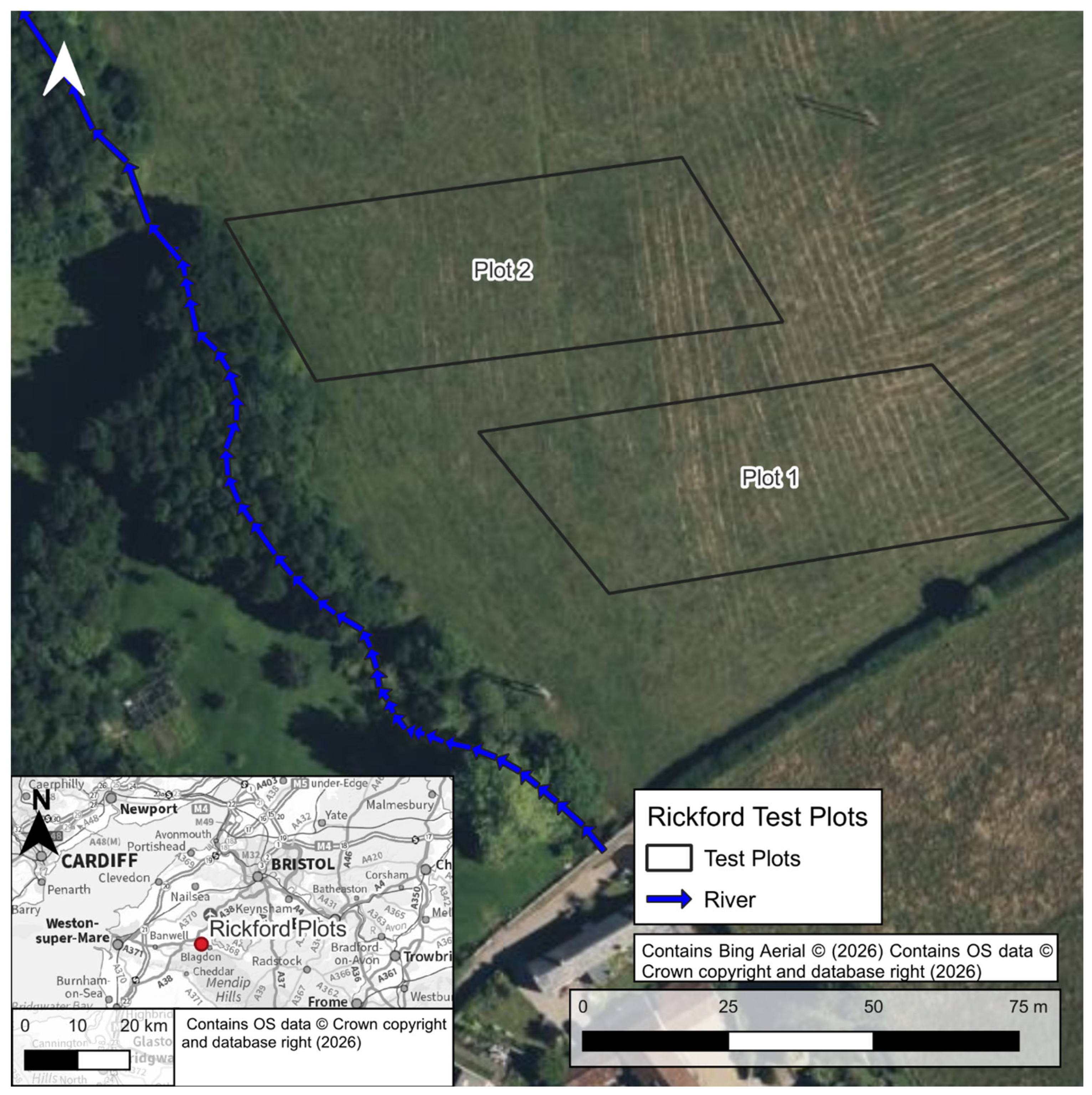
Figure 1 shows two plots, each with a 10 m and 40 m buffer between source and minor watercourse.
At the time of writing the plot-scale calibration data for various contaminants were not available, so an existing published efficacy for Total Phosphorus (TP) has been used as calibration data by way of demonstration of the three modelling approaches, first at the plot-scale and then at the waterbody scale (Fieldmouse and CSF-HYPE).
Natural England [
7] summarise the literature on nutrient removal efficacy (i.e., percentage reduction in initial load at buffer edge reaching the watercourse) based on a literature review for 10 m are as follows, with additional details provided in a supplementary note:
The review covers nitrate as the only nitrogen form, rather than all forms of nitrogen (total nitrogen—TN), along with TP. Only TP is modelled here since agricultural-derived phosphorus is highlighted as a key reason for the catchment not achieving good ecological status. It should be noted that these removal rates are contested in the research literature [
11,
12,
13] and are strongly influenced by site conditions, environmental character, and buffer zone design, including the nature and management of vegetation cover, the prior use and contaminant-saturation status of the soils, and whether the buffer zone feature effectively intersects with dominant flow pathways linking land to stream. The figures here, therefore, are used here as an example of currently reported rates in the UK, rather than an absolute rate likely to be representative of all site conditions.
They include the full width of the buffer strip, i.e., they do not ‘remove’ the efficacy of the first 2 m which is undertaken in England when assuming that farmers are following ‘Farming Rules for Water’ [
14]. If we do want to follow the Natural England approach and ‘remove’ the impact of the first 2 m, then Natural England [
7] suggest the following for 2 m width efficacy:
Meaning that the ‘residual’ efficacy figures, when ‘Farming Rules for Water’ [
14] are followed, for 10 m buffers are:
In this study, we compare with these residual rates to undertake a theoretical simulation of the likely impacts of introducing buffer zones 10 m distance from the stream, on the flux on livestock-derived phosphorus from land to stream.
3. Methods
Here we introduce three open modelling tools to help understand the potential impact of different nature-based solutions on phosphorus transfers from land to stream under UK conditions, across different scales and time periods. These are the particle tracking model, JUMP (v 0.9001), the source-pathway-receptor model, Fieldmouse (v7.5) and SMHI’s unsteady, process-rich HYPE (v5.22) model [
15] and its application to England called CSF-HYPE [
9,
15]. We demonstrate the modelling approaches, how they can be calibrated and explore techniques to explore implications for contaminant transfer to UK freshwaters at the plot, catchment and regional or national scales.
The flow pathways and transport rates in JUMP have been conceptualised in the same way as those in the steady-state Fieldmouse model to permit intercomparison and upscaling from the plot-scale to the catchment scale. The pathways comprise a quick flow (QF) and slow flow (SF) pathways, apportioned based on the local base flow index (BFI). The CSF-HYPE model represents a more complex set of pathways in different surface soil layers although these can be grouped for comparisons. CSF-HYPE has been actively updated with new data and refinements since 2018 with the purpose of evaluating the effectiveness of UK Defra’s programme of catchment sensitive farming (CSF) [
16].
3.1. JUMP
JUMP is a Lagrangian particle tracking model with conceptualised quick-flow/slow-flow hydrological pathways having proportions based on an estimate of the local baseflow index using open data. Particles are initiated in a source zone and undertake the random walk/perturbation to emulate turbulent mixing on the surface, and random pathways in the soil and macropores, with each adhering to a decay rate associated with contaminant being represented. Here we focus on TP, permitting comparisons with the published Natural England efficacy rates [
7] reported in
Section 2 (the model can also initiate particles to emulate particulate and soluble phosphorus forms). Key assumptions on mean velocities, slope and decay rates have been selected to allow comparison with Fieldmouse, the model used to upscale findings from the plot scale to the catchment scale (or waterbody).
A large number of particles (ten thousand used here) representing unit mass of contaminant are initiated from an application area (e.g., where fertiliser is spread) and advected based on the Mannings formula taking into account the local slope from an analysis of the 1 m Environment Agency LiDAR data, and roughness based on a look-up between broad land-cover map, Living England [
17]. The velocity,
, of a particle on the soil surface is computed using Equation (1):
where
R is the hydraulic radius, approximated as depth of overland flow during an event and set to a value of 0.01 m to yield typical overland flow velocities of the order 0.04 m/s within a typical observed range from measurements across a range of vegetation types [
18].
S is slope and
n is the Mannings roughness, based on lookup tables, but typically set at ~0.03 for grassland [
19]. This formula is used to be consistent with the systems-based Fieldmouse model introduced in the next section. Particles are advected using Equation (2):
based on the steady-state velocity field from Equation (1), but including a random perturbation to emulate turbulent diffusion. In Equation (2),
S is a position vector based on X and Y position of the particles at time
t + ∆
t;
is a fixed turbulent dispersion term (0.05 m
2/s quick-flow, and 0.01 m
2/s for slow-flow), scaled a velocity scaling factor,
, depending on the pathway.
, which is set at 1 for surface pathways and 0.01 for sub-surface or slow-flow pathways. The same values are used in Fieldmouse conceptualisation.
The vector of particle positions is stored through time, and the particle mass,
, is also retained with decay based on a half-life,
, using Equation (3):
This formulation is also used in Fieldmouse and is the main calibration parameter for both JUMP and Fieldmouse.
A retardation factor can also be applied to the particle to emulate adsorption processes, but this has been held at unity here for simplicity, so all the variation is in the half-life for comparison with Fieldmouse.
3.1.1. Inputs
Terrain data was prepared at the finest resolution available for JUMP of 1 m. This was based on the Environment Agency LiDAR survey which compared well to a local survey of the Rickford site. For compatibility with the Fieldmouse model, the LiDAR data was used, albeit at the higher resolution of 1 m in JUMP and 10 m in Fieldmouse. A distributed Mannings roughness grid was derived, based on the landcover in NE Living England habitat map [
19], which is derived from Sentinel Earth observations data, and here the site comprised mainly grassland.
3.1.2. Assumptions
An overland flow depth of 0.01 m was used yielding overland velocities of ~0.01 m/s.
The ratio of quick-flow to slow-flow was set at 0.01. This could be determined from additional modelling, e.g., using Richards’ equation, or from in-situ measurements, for example, with monitored throughflow collectors.
Diffusivity—this was set at a small value to promote mixing to emulate turbulent transfer over the micro-topography and change of course in soil structure, potentially influenced by macro-pore and root systems.
3.1.3. Outputs
Breakthrough curves are obtained as the particles enter the line defining the watercourse. It should be noted that some particles for both baseline and scenario runs by-pass the watercourse altogether due to the slope direction, estimated at 5% of the load applied to plot 2 in
Figure 1 based on the number of particles not reaching the boundary). The breakthrough curves can then either be plotted using particle count (no decay) or by integrating the decayed mass to permit comparisons between different assumptions such as the reduced velocities from increased vegetation in the buffer strip. Here the decayed TP load used the calibrated half-life from the Fieldmouse simulation (5 days), although of course this is a simplification of its speciation to permit comparison with empirical data.
3.2. Fieldmouse
Fieldmouse is a steady-state systems-based model designed to simulate the movement of diffuse pollution at the field scale, tracing its journey across the physical landscape to local watercourses. This approach facilitates the evaluation of measures to enhance farm management practices and considers both topographical factors and conceptual pathways for QF and SF to the river network and a downstream point of interest (POI). Developed in collaboration with the Environment Agency since 2014, Fieldmouse has evolved into a freely distributable QGIS python-plugin [
20] supported through JBA’s R&D investment in 2022. The model is reported here for the first time providing details on the key assumptions.
For efficiency and sufficient spatial detail, Fieldmouse adopts a 10 m landscape resolution. Broadscale agricultural pollution loads, summarised from Farmscoper v5 [
21] (which uses 2019 land use and 1981–2010 climate data) are disaggregated using land-use (Living England), climate (HadUK), and soil class data [
22] via open-data classification at operational water management catchment scale.
Landscape connectivity is mapped using geo-spatial hydrological processing, with a DTM outlining connections between each pixel and river network, here based on the Openrivers dataset, a topologically connected open dataset of the river network for Great Britain [
23]. Flows and pollution are routed through every network segment to a chosen POI, such as a catchment outlet. The local flow is estimated based on the accumulation of the distributed runoff which has been estimated based on the water balance method, and a global scaling parameter is applied to ensure the total at the outlet agrees with the long-term mean gauged flow.
Surface transport rates are governed by slope and roughness, simulating land-phase pathways and are scaled for slower sub-surface pathways, while pollution decay is modelled according to travel time and user-defined half-life. Upon entering the river network, empirical equations based on broadscale tracer-tests [
24] determine transport rates in terms of average velocities, with further decay calculated along the route to the POI. All model data inputs and parameters are specified through a detailed, annotated spreadsheet which provides a useful record of the locations of the complex spatial datasets.
After determining the decayed load at the POI, Fieldmouse performs ‘reverse’ calculations to apportion the POI load back to every pixel using new rasters. The initial processing also generates a Time of Travel (ToT) raster, summarising cumulative travel time from any pixel to the river network and along the network to the POI. When combined with user-specified loss rates for both land and river phases, this enables the decayed POI load to be attributed back across the landscape, resulting in a spatial unit response function, here called an importance raster. The importance raster quantifies the expected decay of pollution from each pixel at the POI and assists in identifying areas to avoid for new diffuse pollution inputs.
Multiplying the importance raster by a raster of pollution load (from disaggregation of for example Farmscoper excess loads) yields a spatial estimate of the decayed contribution from each pixel to the POI, known as the pollution risk raster. This tool is invaluable for pinpointing locations where spatial interventions will be most effective. Targeted reduction strategies, such as adjusting input loads on the highest-risk 10% of arable pixels, can be readily assessed by recalculating expected reductions with the importance raster. Physical landscape modifications, like introducing buffer strips, can be modelled as changes in roughness, which impact both ToT and pollution losses, further refining the importance raster. Collectively, use of these rasters permits the testing and optimisation of diffuse pollution mitigation strategies.
3.2.1. Data Inputs
The river network was represented using the best available topologically correct open data, identified as being the Openrivers [
23] dataset and later refined. This was used in combinations with the widely available Water Framework Directive (WFD) surface waterbody polygon data to define the watershed. Distributed runoff was developed against a finer set of watersheds within the waterbody using the water balance method and dividing the quick-flow, slow-flow response using the Baseflow Index derived from local NRFA sites using the UKFE R package [
25]. The annual average distributed agricultural diffuse excess nutrient loads are based on Farmscoper v5 upscale [
21]. This was first simulated for the wider water management catchment and then disaggregated based on Natural England’s Living England landcover map derived from Sentinel for 2021 [
19]. The disaggregation was undertaken incorporating the landcover class, and five soil texture classes (fine, medium, heavy, chalk and organic) based on British Geological Survey open soil texture classes, and the climatology [
22]. In addition to these spatial datasets, some calibration parameters are provided by the user in the input spreadsheet—the key ones being the land-phase half-life and a decay rate representing in-stream losses.
3.2.2. Pre-Processing and Forward Calculation
The Fieldmouse pre-processing tools are used to develop the key information required by the transport calculation, including the network connectivity, stream order and stream-slopes based on the DTM. The forward processing model is then set up with the required input datasets described above, with any unit conversions handled to ensure the outputs are in SI units.
Flows and entrained substances are considered to follow two pathways in the same way conceptualised for JUMP, i.e., quick flow and slow flow pathways. The quick flow pathway corresponds approximately to direct surface runoff and fast sub-surface runoff pathways in the upper soil layer. The slow flow pathway covers all deeper sub-surface and groundwater flow pathways.
The overland velocity is based on the Mannings Equation (1), with a user-input overland flow depth (set at 0.01 m as per JUMP) and the sub-surface transport is assumed to follow the same pathways as the surface, but with a reduced velocity, here using the 0.01 factor and a proportion based on the baseflow index (BFI), as per the JUMP simulation.
The river network is made up of segments between confluences or nodes with attributed topology (upstream-downstream connectivity). A given cell in the landscape can only drain to one segment and for a given segment there will be zero or more cells that drain to it. The collection of cells that drain to a given river segment form a sub-catchment or watershed for that segment. The model therefore works with a series of river segment-watershed pairs, and the river-segments are the finest resolution scale at which flows and loads are computed.
Fieldmouse makes use of efficient in-built GIS hydrological processing tools (PCRaster toolbox) which provide an integrated response at each river segment. It requires the user to provide a 10 m resolution, sink-filled DTM to permit connectivity between each pixel and the catchment outlet. Fieldmouse generates a flow direction grid (8-directional scheme) and uses this to generate watersheds draining to every stream-segment such that every pixel is indexed with the segment it will pass flow and pollutants to, via the hydrological pathway. The pathways lengths from every pixel to the receiving stream segment are computed using the hydrological pathway length (HPL) tool computing the most probable pathway each pixel in a watershed is linked to its corresponding river segment.
The watershed tool is initially used to accumulate the distributed estimate of runoff (QF and SF) reaching each river segment. These flows are then accumulated in a stream-ordered calculation through the river network down to the outlet or a POI where there is a flow gauge. Here the mean flow from a long term NRFA flow gauge (S2017—Congresbury Yeo at Iwood) is used to calibrate a catchment-wide runoff-scaling factor such that the accumulated distributed runoff agrees with the long-term mean flow of 0.802 m3/s.
The HPL tool is used to derive a travel-time for each pixel by using an impedance-weighting (1/velocity) to generate a cumulative travel-time grid from any pixel to associated river segment to the POI. Combined with a constant substance half-life and using the same form of Equation (3), the decayed accumulated load reaching each river segment is obtained highly efficiently. The total pollutant load entering a given river segment is the sum of the contributions from each cell that drains into that segment—that is from the watershed for that river segment.
Once the decayed accumulated load from each watershed reaches its associated river segment, the calibrated accumulated runoff is used to estimate the local concentration, and instream processing is undertaken. This follows a similar travel-time and decay approach but is ordered from headwater to outlet as follows. Starting with stream-order 1 (SO 1) river segments the decayed accumulated loads (from both pathways) are decayed assuming an in-river travel time. This time the in-stream velocities are based on an empirical equation developed from rhodamine tracer experiments across England [
24] given by Equation (4):
where
;
is the slope;
is the mean flow and 86.4 is a factor required to convert into SI units.
Here slope () has been determined from the pre-processing tools and the change in elevation, and the mean flow () at that location, based on the accumulated runoff to that river segment. Combined with the river segment length, the travel time for each segment is estimated, and for loads arriving from the associated watercourse half the distance is assumed.
The SO 1 travel time and decay losses are first computed, and the SO 2 computations are undertaken- taking all contributing stream-order 1 decayed loads and flows and decaying these by the full travel time, plus the watershed contributions from the associated SO 2 segments are accumulated and decayed assuming the half-river segment pathway. This is repeated until the highest SO is reached and for each segment the flow, undecayed load, decayed accumulated load to that point and resulting in-stream concentration are computed for each pollutant.
3.3. HYPE
HYPE (HYdrological Predictions for the Environment) is a hydrological and water quality model developed at the Swedish Meteorological and Hydrological Institute (SMHI) [
15]. The model is open-source and semi-distributed. HYPE is supported by a large wiki and community of users, and working collaboratively with SMHI and the Environment Agency, JBA helped to develop a new version to help evaluate the effectiveness of Catchment Sensitive Farming (CSF) called CSF-HYPE [
9]. The national CSF-HYPE for England differs from the above models since it represents many more processes and incorporates multiple sources of pollution, including continuous and intermittent sewage discharges, septic tanks and some allowance for animal defecation directly into the watercourses.
3.3.1. Data Inputs
The HYPE model is driven by meteorological forcing data comprising daily catchment averaged precipitation and air temperature time series based on the HadUK 1 km gridded, long term record [
26].
Point source discharge data (flows and concentrations) were based on Environment Agency returns of treated effluent concentration and flows where available or consented discharges where not monitored. Key flow abstractions were based on three Environment Agency databases. Diffuse excess load data was based on EA data, which combines loss coefficients derived from the same ADAS Farmscoper v5 model used by Fieldmouse, with Defra land use data covering the period 2000–2021 and annual HADUK 1 km gridded precipitation data [
26]. Excess pollutant loads were aggregated and anonymised from farm-level data into a monthly timeseries of average daily total excess pollutant load per broad land use class within each CSF-HYPE Hydrological Response Unit (Defra License).
Flow calibration data was based on daily flows over the years 2000–2020 and across 777 NRFA flow gauges [
27]. Water quality calibration was originally across 14,800 Water Information Management System (WIMS) water quality sample points [
28]. Spatial river network and lake data are based on available Environment Agency datasets
3.3.2. Process Summary
The HYPE model begins by converting the forcing data inputs of rainfall and temperature into hydrological responses such as snowmelt, evapotranspiration, infiltration, and runoff, which together determine how water enters and moves through the landscape. As precipitation infiltrates the soil layers, the model simulates soil moisture dynamics, groundwater fluctuations, macropore flow, tile drainage, and lateral flow, while simultaneously tracking other nutrient pools (e.g., organic N/P, inorganic N species, soluble reactive P fractions) within each soil compartment. Water and associated nutrient loads from each hydrological response unit (see below) then enter local streams and lakes, where the model routes flows via conceptualised river attenuation routines and lake mixing processes, transforming nutrients through processes such as mineralisation, settling, adsorption, and decay. Nutrient dynamics in rivers and lakes are represented explicitly, with HYPE modelling inorganic nitrogen, organic nitrogen, soluble reactive phosphorus, particulate phosphorus, and sediment–nutrient interactions as they travel downstream, including transformations within both the water column and benthic sediments. Finally, these flows and nutrient concentrations are routed along the main river network toward the basin outlet, integrating contributions from upstream soils, tributaries, lakes, groundwater, and point sources, enabling assessment of diffuse pollution, nutrient retention, and catchment-wide water quality responses.
3.3.3. Soil-Land-Travel Band Classes
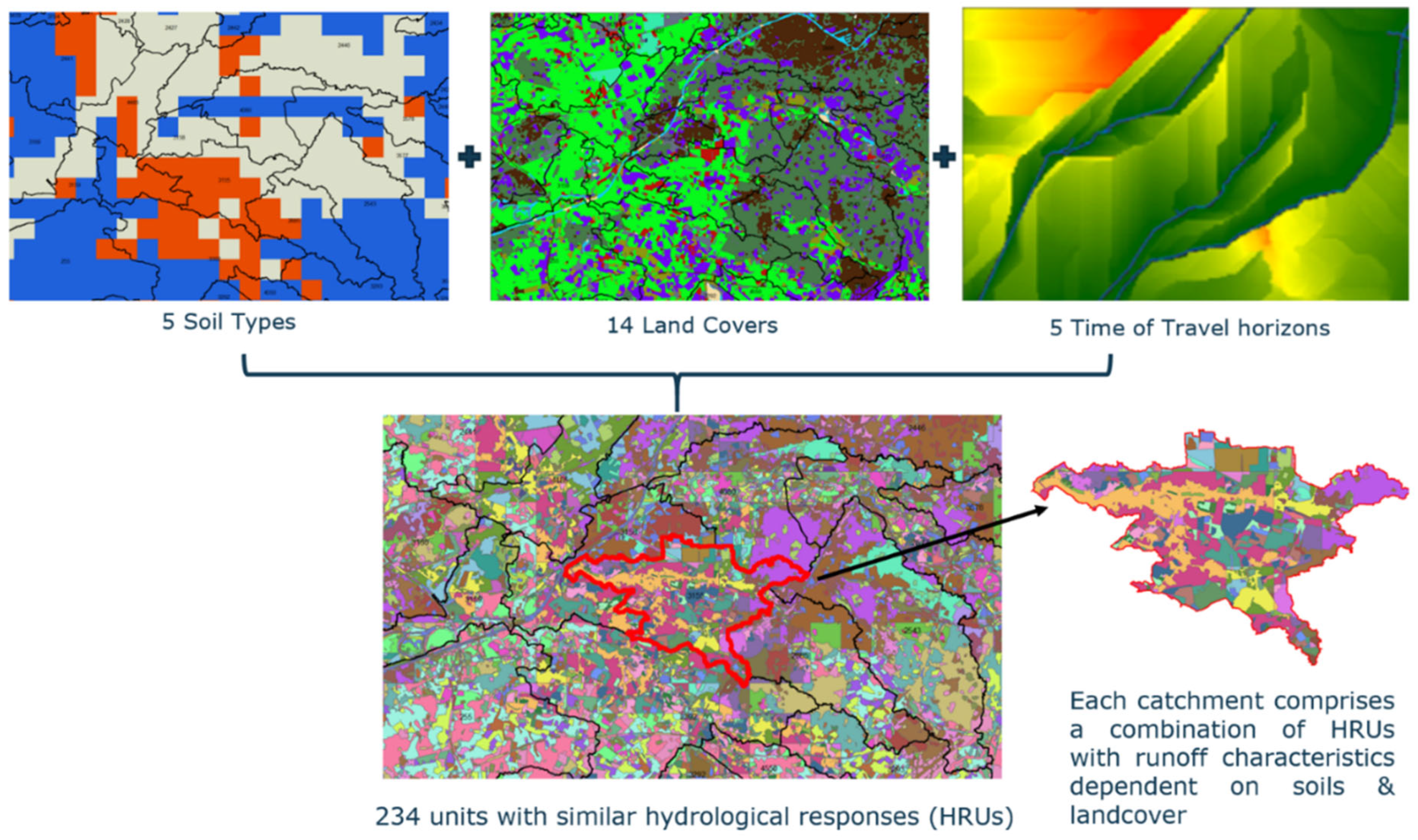
Unlike JUMP and Fieldmouse, CSF-HYPE is not fully distributed and relies upon breaking the landscape down into soil-land classes (SLCs), sometimes called Hydrological Response Units (HRUs), based on: 5 soil texture classes; 14 land-use classes; and 5 travel-time bands (
Figure 2). These generate runoff based on calibration of each soil-land use class combination, and this is routed via a conceptualised local river network, before reaching the main river network in which sedimentation, macrophyte uptake, and other processes are represented.
The travel-time bands were introduced in CSF-HYPE [
9] to allow for some representation of the effect of different hydrological pathway lengths for diffuse agricultural sources of pollution depending on their distance from the stream network. This property is not used in hydraulic parameter calibration and only influences pathway travel-time, but they are made use of here to target higher risk areas with shorter travel times for soil and land-use improvements, as opposed to explicitly representing buffer strips in the SLCs which would require major reformulation of the model.
4. Model Scenarios
The model scenarios have been set up with the aim of understanding the loss rates (in terms of half-life) and velocities required to achieve widely reported nutrient removal efficacies of different NbS, first at the Rickford plot scale, then at the Yeo catchment scale and more widely across England. Here the focus is on TP since this has been a key chemical resulting in failure of Good Ecological Status, but the approaches will be adapted for other pollutants as data becomes available. JUMP and Fieldmouse simulations are both dependent on calibrating an appropriate half-life for TP to yield the observed concentrations at the nearest downstream EA water quality monitoring point since this represents the key empirical evidence available.
4.1. Calibration of Half-Life
The Fieldmouse calibration takes a multi-step process, first ensuring a flow balance. The first step comprises estimating a flow scaling factor by comparing integrated flow at outlet to nearest flow gauge with long-term record (Congresbury Yeo at Iwood, Station 52017). For the study-catchment, a factor of 0.4 was required to scale the distributed runoff to match the long-term average of 0.802 m3/s at this gauge and ensure the correct dilution.
Having attained a flow balance, the TP decay rates (land-phase and instream) were calibrated against the appropriate long-term average concentration at the closest downstream site (E8101000) having a mean concentration 0.236 mg/L soluble phosphorus (SP) over most recent stable period in data 2011–2020. Since the investigation only assesses diffuse sources, this measurement has been adjusted to reflect the long-term average estimated agricultural source apportionment of 40%, giving a target calibrated concentration of 0.094 mg/L for SP, scaled to estimate TP by a factor used in national model of 1.11, yielding 0.104 mg/L.
The in-stream TP decay rate was set at 0.25 day
−1, which corresponds to a half-life of 2.8 days and is typical of the rates used in, for example, national SIMCAT modelling [
29]. The land-phase half-life was then calibrated at 5.0 days to meet the target downstream concentration within 3%. The same land-phase half-life was assumed for the particle loss rate in JUMP for baseline and buffer-strip scenarios, with the latter represented using an increased roughness within a 10 m buffer.
4.2. JUMP Simulations
JUMP Riparian Buffer Strip Scenario, J1
The riparian buffer strip scenario in JUMP simply increased the Mannings roughness within the buffer strip area between plot 2 and the water’s edge in
Figure 1, to slow the quick flow, and proportionately, the scaled slow flow. This results in a longer travel time and combined with the baseline half-life incurs increased decay. A comparison was made between the peak concentrations in the breakthrough curves predicted by the baseline and roughening-up scenario. In reality, other processes such as retardation and transformation occur, but here the loss is a pure exponential decay with the calibrated half-life.
4.3. Fieldmouse Simulation
Fieldmouse Riparian Buffer Scenario F1
In combination with the calibrated half-life of 5.0 days, a riparian buffer strip spatial scenario was developed (
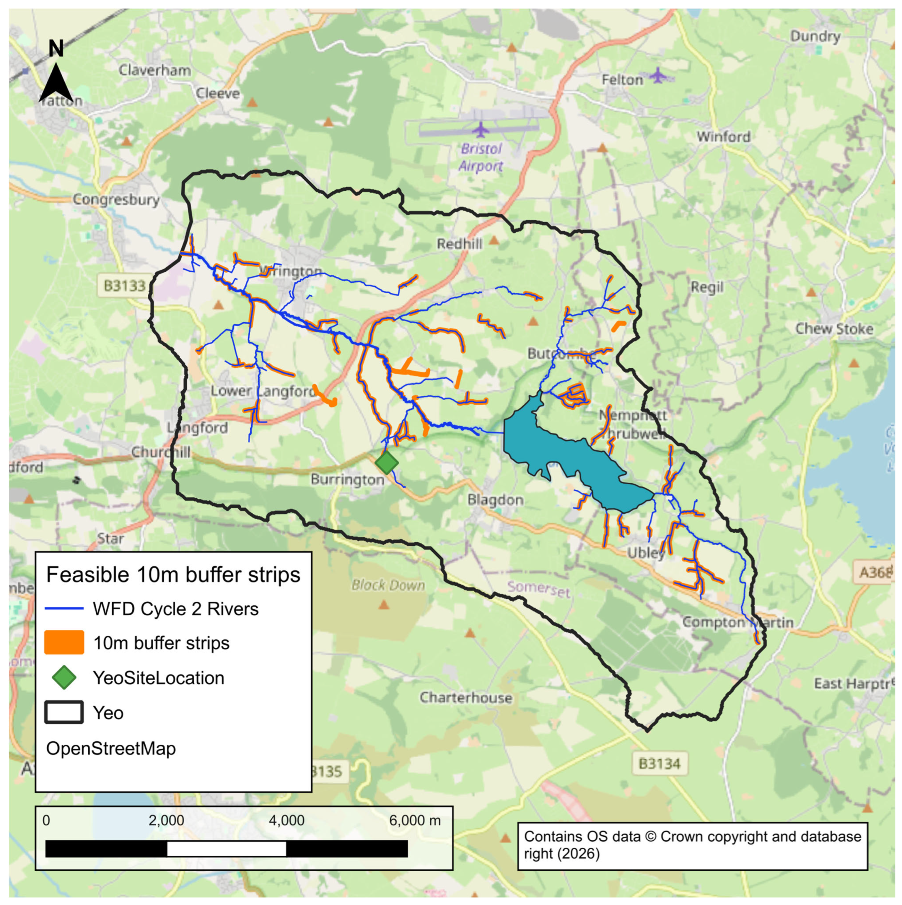
Figure 3). This can be set using the risk-grid output as a useful form of prioritisation, but here all grassland was targeted that was not infrastructure, hard-standing or woodland.
Figure 3 shows the spatial strategy for the Yeo based on 10 m buffer strips on grassland and improved grassland, comprising a total area of 52.9 ha, which represents approximately 45% of the total length of watercourse using the Openrivers dataset. The reduction in the load at the outlet for this strategy was tested, varying only the roughness within these defined buffer-strips to emulate establishment of vegetation.
4.4. CSF-HYPE Model Scenarios
4.4.1. Baseline HYPE Model Calibration
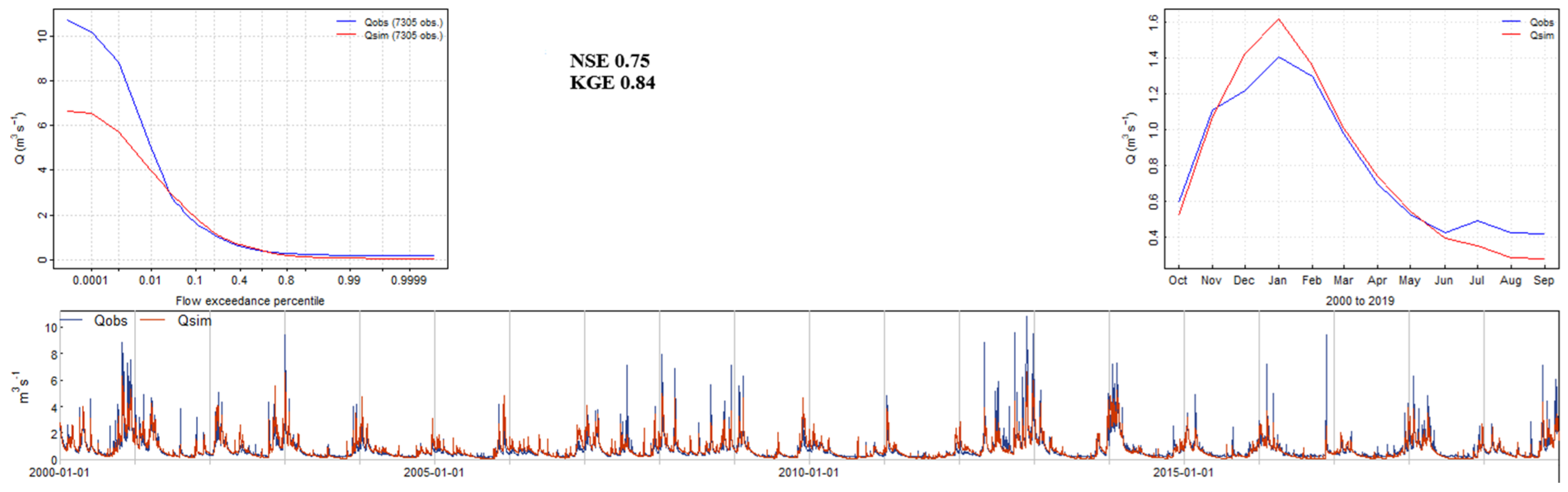
As a first step the Yeo sub-basin was split off the national CSF-HYPE model, and the daily flow calibration was improved for flows over the national calibration, for the simulated period 2000–2020 (
Figure 4), yielding an NSE performance measure of 0.84, and this was used with the existing national calibration parameters for the baseline simulation with CSF-HYPE, to compare against a sustainable land management (SLM) scenario described below.
4.4.2. HYPE Sustainable Land Management Scenario H1
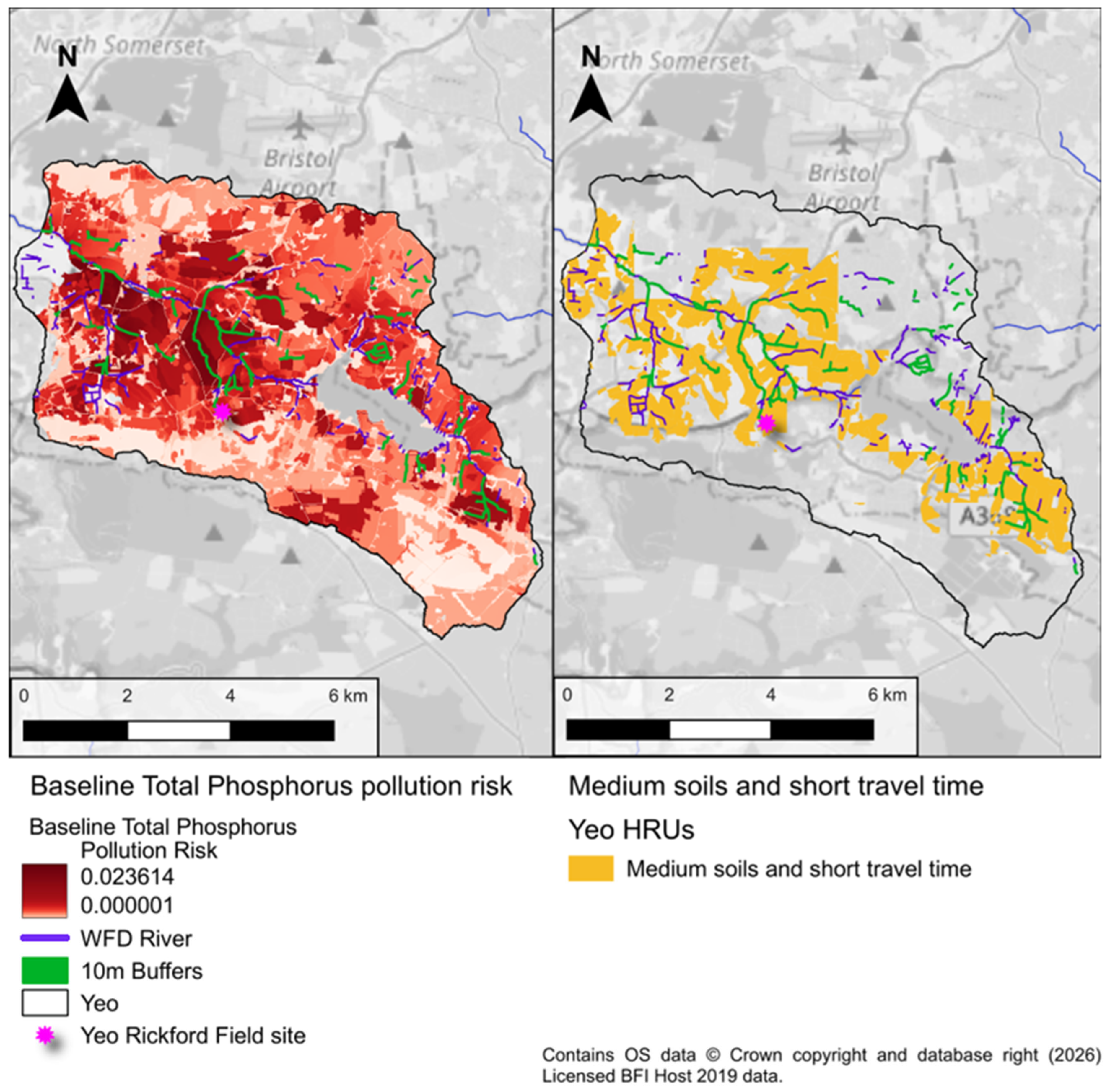
A comparison is first made between the higher risk areas identified using the Fieldmouse risk-grid and areas targeted in this way for a reduction in agricultural load due to Sustainable Land Management for shorter travel-time classes (
Figure 5). The risk map is an output from Fieldmouse and considers the distributed agricultural load (source) and the connectivity in the landscape (pathway).
Qualitatively, the targeted areas in the shorter-travel time bands correspond with the higher risk areas based on the Fieldmouse risk analysis and represent a useful strategy at the catchment scale, although there are differences between the open-data loads used in Fieldmouse and those in the CSF-HYPE model since this latter has access to higher resolution, licensed data. The zones targeted for SLM here correspond to the short travel time band; Improved Grassland or Arable; and Medium Soils
In the orange areas identified in rightmost image in
Figure 5, a suitable TP reduction scenario was required for which there have been numerous efficacy values published across a range of SLM improvement types. In one meta-analysis paper [
30], it was estimated that riparian buffers can reduce TP loads by 30–85% depending on width and slope, while others have reported an increase or no net decrease in TP loads under other circumstances [
11,
12]. The NE range used in this study falls within this range and suggests a 30 m buffer can reduce fluxes to streams by up to 89% for TP, or 42% residual efficacy if we assume 2 m buffers are already in place from adherence to Defra Farming Rules for Water [
12].
For the purposes of this modelling experiment, we assume riparian buffer strips in these identified zones will result in a 45% reduction in TP delivered to the water based on the mean of the broad range in the literature. A direct comparison was then made between the concentration and cumulative loads at the outlet of the catchment between this reduced load scenario and the baseline model using the national calibration (CSF-HYPE version 6.02).
4.4.3. HYPE Scenario H2: National Upscaling of Scenario H1
Finally, the above classes and 45% efficacy was rolled out in the national model to understand the range of reductions possible across different catchments, typologies and climates in England based on the existing national calibration.
5. Results
5.1. JUMP
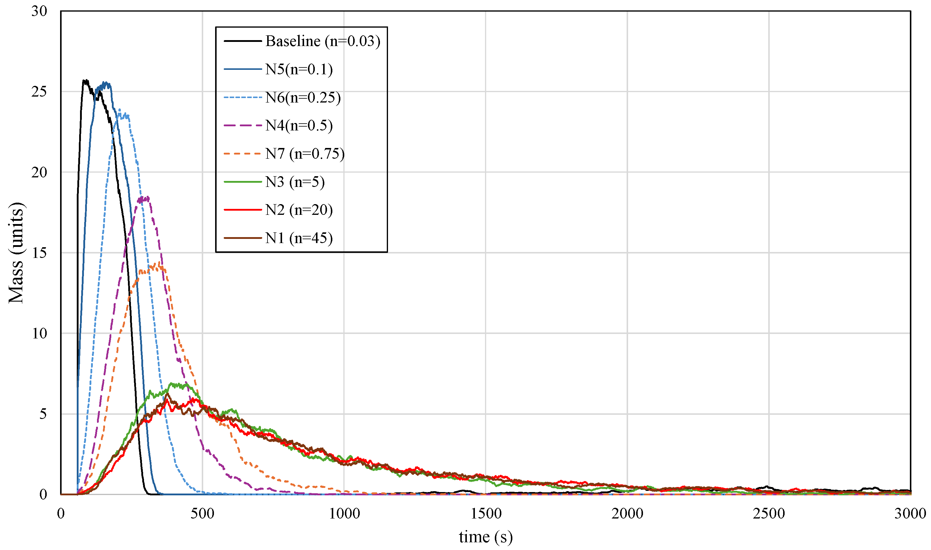
The JUMP model was simulated using the same half-life for TP that was calibrated using the Fieldmouse model (5.0 days), and the roughness was increased using a wide range of Mannings number until the breakthrough curve showed a reduction supported by the published literature. It should be noted that the baseline roughness for grassland was assumed to be n = 0.03, and extremely high values were used outside physically realistic range to permit very slow velocities (
Figure 6).
The breakthrough curves shown in
Figure 6 were smoothed using a moving window of 60 s to reduce noise and avoid longer runtimes. Assuming good farming practice is in place (Farming Rules for Water [
14]), the N4 breakthrough curve yields a peak polutograph concentration reduction of approximately 27.8%, requiring an increased roughening up that is physically plausible for
highly vegetated and complex terrain (n = 0.5 or velocity ~ 0.01 m/s). Assuming higher values of efficacy (such as no existing buffer), requires unrealistic roughening up greater than this (breakthrough curve N1; velocity ~ 0.0001 m/s), although this current model does not consider factors such as retardation due to bonding and transformation. As the window over which the efficacy is computed is reduced to 2 min the efficacy in terms of ‘peak mass avoided’ reduced to 8.1% and then 1% beyond 5 min for the same roughness (n = 0.5). It is important to consider the implications, for instance, if the release of the particles represent an incidental rainfall event following application of, for example, manure, much of this will reach the watercourse in the current setup over time, but significantly reducing peak concentrations will be more important for chemicals with more acute ecotoxicological impacts.
5.2. Fieldmouse
The calibrated baseline Fieldmouse model was next used to simulate and upscale the catchment scale impact of 10 m buffers shown in
Figure 2 in terms of TP reduction at the outlet. The calibrated half-life the model was repeatedly simulated increasing the Mannings roughness in all buffers to slow the flow and permit more time for losses across the buffer strips. For a small, buffered portion of grassland headwater (unaffected by upstream loads), Fieldmouse shows a 7.3% reduction in load arriving at the watercourse over a non-buffered baseline when using the same change to roughness (n = 0.5) that were calibrated using JUMP. Whilst JUMP yielded a 27.8% peak reduction, this reduced to 8.1% ‘peak mass avoided’ when using time-averaging centred on the peak, and less when integrated over the whole event.
At the whole catchment scale, and measuring change at the catchment outlet, the Fieldmouse model shows 5.0% reduction. This is in much part due to the reality of feasible catchment-scale implementation of buffer strips (
Figure 2), considering a realistic spatial strategy resulted in 45% of the network length to be buffered, the distribution of agricultural loads in the catchment. The concept of ‘catchment-scale’ efficacy (for realistic spatial strategies) could be very useful in combination with the notion of buffer-strip efficacy for management purposes.
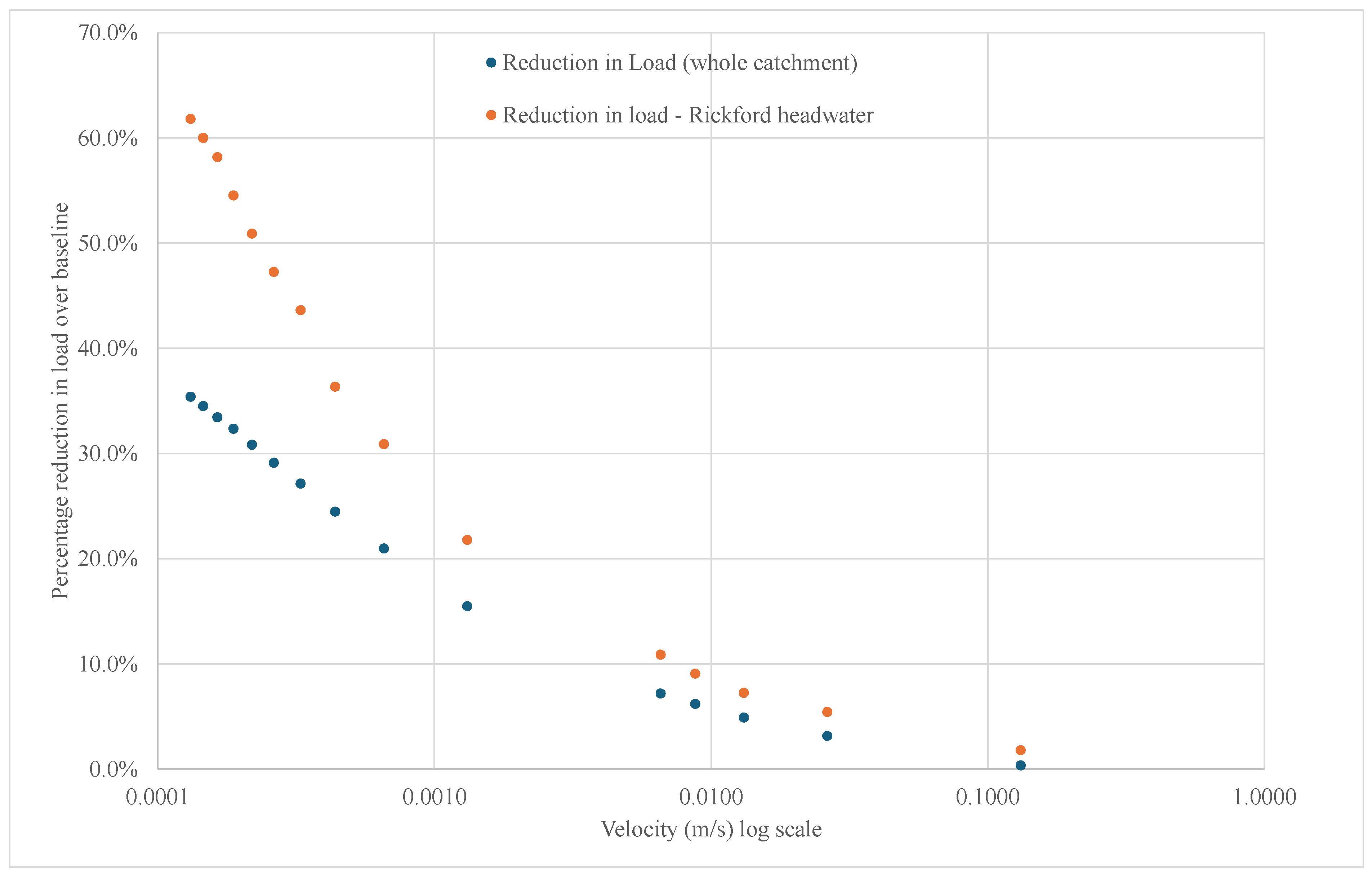
For catchment scale efficacies close to the plot scale, with feasible spatial strategies, much greater increase in roughness and corresponding reduction in velocity would be required -approximately 300-fold, as opposed to the 10-fold identified using JUMP to achieve the types of efficacies (
Figure 7), implying other processes are taking place.
Figure 7 also shows there is a marked kink in the efficacies for both a small headwater catchment and at the catchment scale as slower velocities and higher travel times are attained (<0.001 m/s). The figure also suggests that above this apparent threshold the change in velocity over baseline does not make a significant difference. For a 10 m buffer, the 0.001 m/s equates to a travel-time of approximately 2.8 h, or 2% of the calibrated half-life (5 days).
5.3. CSF-HYPE
5.3.1. CSF-HYPE Scenario H1
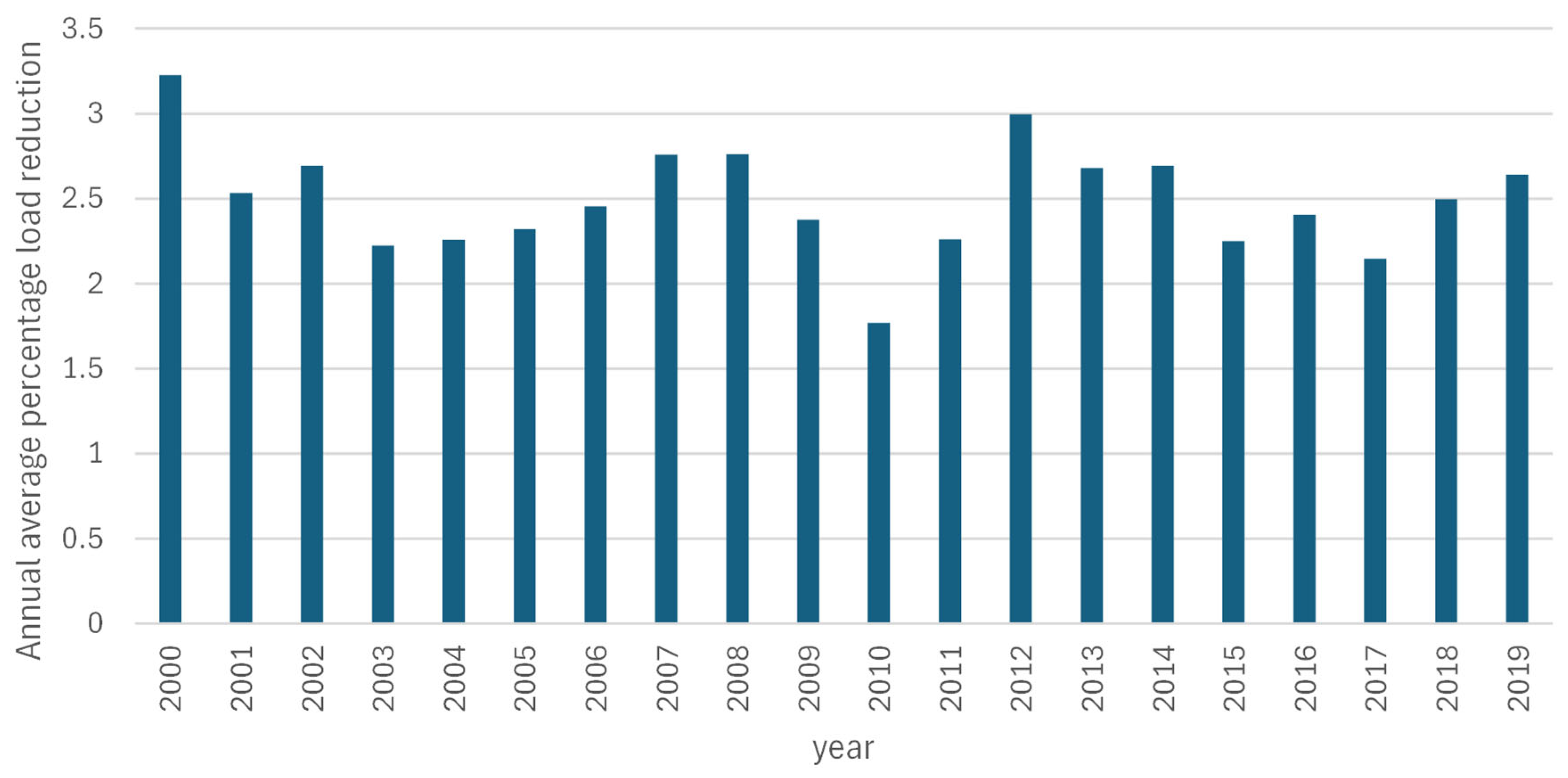
For CSF-HYPE scenario H1, the long-term average cumulative load reduction as a percentage of total load at the catchment scale was estimated to be 2.5% over the 20 years of simulation (
Figure 8). This equates to a larger reduction of 6.3% of the total load (considering point and diffuse sources), which is similar to what was observed with Fieldmouse at the catchment scale in terms of reduction in diffuse load (5.0% reduction).
Closer inspection of the targeted classes for excess load reduction for scenarios H1 highlighted that the two SLC-classes selected for modification (improved grassland OR arable for travel-time band 1, and moderate soils) only receive a small proportion of the total agricultural diffuse excess load based on the HYPE load files. The existing catchment distribution of loads and the spatial strategy strongly influence the overall catchment scale efficacy. Additional analysis including an analysis of through-time source-apportionment was undertaken to explore this scenario more in the discussion.
5.3.2. CSF-HYPE National Upscaling Scenario H2
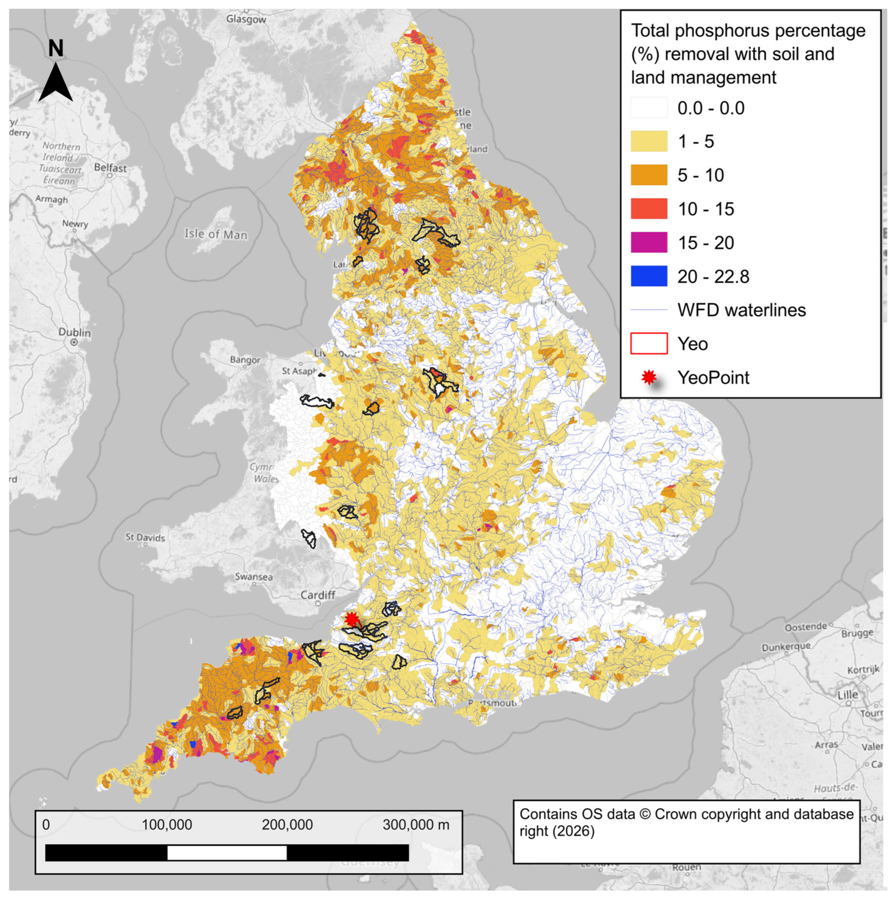
For national upscaling, the results are, of course, dependent on local soils and conditions, the distribution of loads, feasibility, and a large range of assumptions need to be made. Here the same SLM scenario on medium soils was rolled out nationally in
Figure 9, highlighting the spatial variation in catchment-scale efficacy and overlaying QUANTUM spot sampling sites highlighted in black. This demonstrates how catchment-scale experiments can be upscaled nationally using the national CSF-HYPE model, which will permit an understanding of how local field results may change depending on a range of typological factors, intrinsic to the CSF-HYPE classes.
6. Discussion
This article has sought to introduce three freely licensable models (JUMP, Fieldmouse and HYPE, although CSF-HYPE has licensable data) with different complexities to support investigation of the efficacy of riparian buffer strips as a form of nature-based solution. The three models provide useful tools for multi-scale modelling and upscaling from plot-catchment-national scales and highlight the need to discuss plot-scale and feasible-catchment scale efficacy values, since buffers cannot be included everywhere in practice. In summary:
JUMP shows only modest TP retention for realistic vegetation, with peak reductions of ~28% but whole-event reductions of ≤8%. Using a calibrated TP half-life of 5 days, JUMP required a substantial increase in roughness (to n = 0.5) to obtain a 27.8% reduction in peak concentration for a 10 m buffer strip. However, when integrating over longer time periods, the reduction fell to 1%, indicating limited mass removal except at the absolute peak.
Fieldmouse predicts far smaller catchment-scale TP reductions from the same buffer strategy, i.e., only 5% at the outlet despite 45% of streams being buffered. A spatially realistic 10 m buffer implementation covering 52.9 ha (≈45% of stream length) reduced total TP load at the catchment outlet by only 5.0% under steady-state conditions, even when applying the same roughness increase (n = 0.5) used in the JUMP runs.
Direct comparison shows JUMP predicts approximately 4 times higher plot-scale peak reductions than Fieldmouse achieves at catchment scale for the same hydraulic assumptions. Under identical assumptions (10 m buffer; n = 0.5; TP half-life = 5 days):
JUMP: 27.8% peak concentration reduction (plot scale), but much lower when mass-integrated.
Fieldmouse: 7.3% load reduction for a small-buffered headwater and 5.0% at the catchment outlet.
This demonstrates how plot-scale hydraulic efficacy collapses when diluted by spatial feasibility and upstream loading at catchment scale. Furthermore, achieving plot-scale removal rates at catchment scale would require roughly 300-fold velocity reductions; it is considered that this may have to be explained by other transformations or processes that cannot be represented through a friction increase alone. Fieldmouse simulations also show that matching high literature TP removal rates across the catchment (e.g., 70–90% for 10–30 m buffers) would require flow velocities of <0.001 m/s, equating to a 300× reduction from baseline—well beyond what vegetation roughness can generate. The model exhibits a threshold where further velocity reduction provides little additional benefit.
National CSF-HYPE upscaling shows TP reductions of 0–23% depending on soils, travel times and land use, but only ~6% is achievable in the Yeo under realistic targeting. Applying a 45% TP reduction in short travel-time, medium-soil agricultural classes produced:
6.3% reduction in diffuse agricultural load in the Yeo,
2.5% reduction in total cumulative load over 20 years at the outlet,
0–23% reductions when applied across all English catchments in the national model.
The broader riparian buffer strip literature reinforces the central conclusion of Johnes et al. [
12] that nutrient-mitigation performance is governed by complex, spatially variable hydrological and biogeochemical pathway interactions rather than by buffer presence alone. Studies of riparian buffer strips show similarly high context-dependence: Cole et al. [
31] demonstrate that buffer efficacy is strongly modulated by vegetation structure, soil saturation, hydrological connectivity and long-term nutrient loading, with saturated buffers even switching from sinks to sources under certain conditions. Their review emphasises that riparian buffers cannot be treated as simple end-of-pipe solutions and must instead be embedded within catchment-scale management frameworks, as localised retention rarely translates linearly to whole-catchment load reductions.
These conclusions are further reinforced by Stutter et al. [
32], whose synthesis highlights persistent uncertainties around pollutant trapping mechanisms, strong seasonal variability in retention processes, and the risk of over-generalising nominal trapping efficiencies. They argue that assumptions about buffer functioning often ignore pathway-specific behaviour, antecedent wetness conditions and legacy nutrient stores, and warn that the apparent short-term retention observed in some studies may not translate to sustained long-term nutrient reduction. Stutter et al. therefore similarly call for moving beyond plot-scale metrics toward a more process-explicit understanding of hydrological connectivity, residence times and landscape configuration when assessing buffer strip efficacy.
These findings mirror the behaviour observed in our multi-model framework: JUMP identifies only modest plot-scale retention except under unrealistically slow velocities; Fieldmouse demonstrates substantial dilution of plot-scale gains when catchment connectivity and feasible implementation extent are considered; and CSF-HYPE highlights the dominance of hydrological regime and source distribution in determining net outcomes. Together, these studies provide a strong, buffer-strip-specific basis for our argument that effective mitigation requires explicit treatment of hydrological pathways, spatial feasibility and catchment context rather than reliance on nominal plot-scale efficacy values [
12,
31]. Incorporating insights from Stutter et al. [
32] further strengthens this argument by demonstrating that without explicitly accounting for pathway-specific processes, seasonal responses and landscape-scale connectivity, buffer strip performance is likely to be over-estimated.
Each of the three models discussed here will be further developed to improve these shortfalls in process representation and calibration, starting with calibration of JUMP to represent different classes of pollutant behaviour (e.g., conservative, reactive). However, one approach is also to interrogate the model through-time behaviour when considering different sources of pollution, which is next described for HYPE.
Through Time Source Apportionment
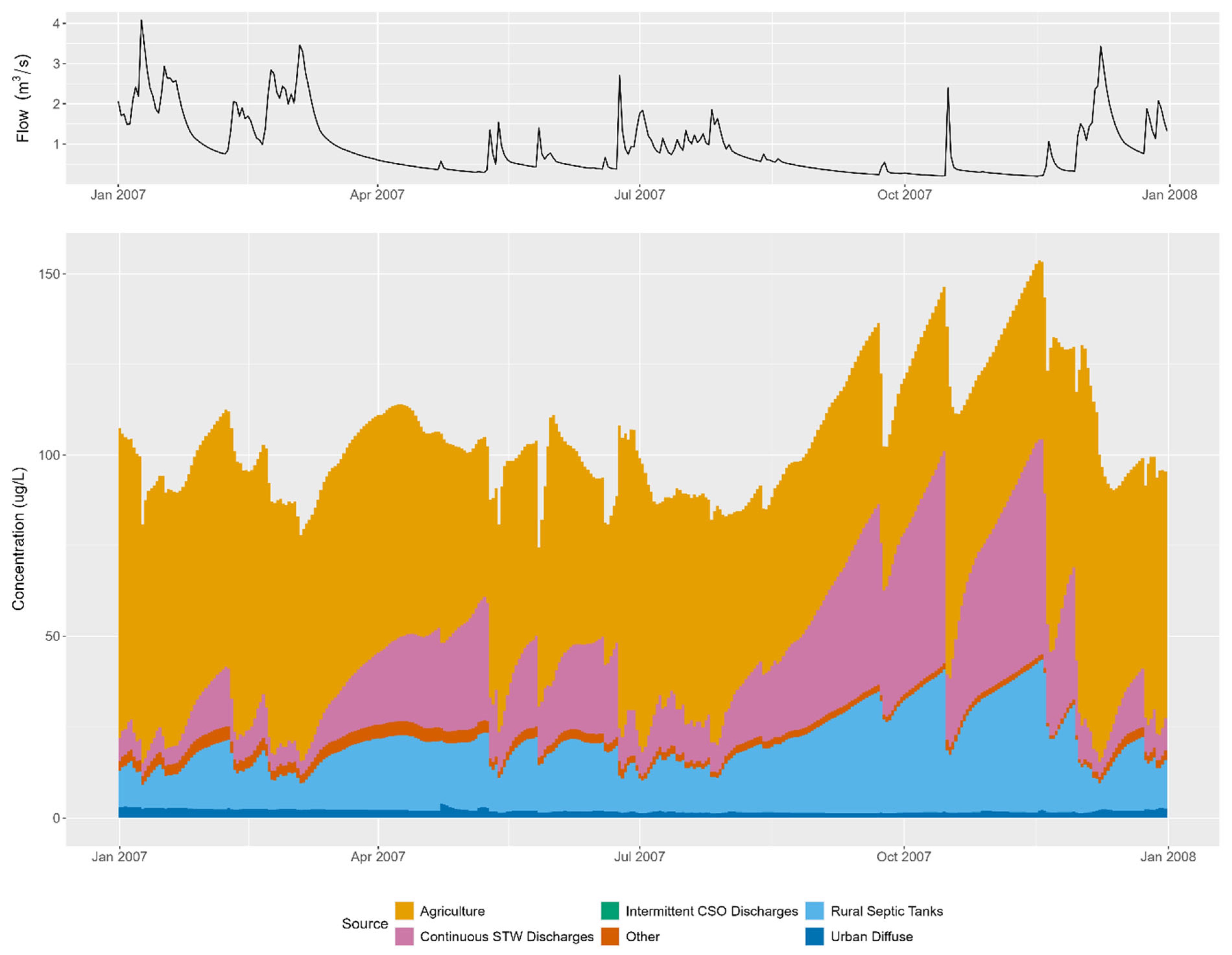
The through-time event-driven or episodic transport of diffuse pollution can be further enhanced with the use of a more sophisticated time-varying velocity field imported to JUMP. However, since HYPE considers unsteady state, albeit with a daily time step, it has been possible to develop new ways to help understand through-time source apportionment. In this technique, the CSF-HYPE model was run repeatedly, sequentially switching off loads from all sources apart from one at a time. Following this the superposition of the polutographs (
Figure 10) is in proportion to the instantaneous load since concentrations are all computed under the same flow conditions.
Figure 10 shows that during higher flows (e.g., January to March for the year 2007) the load from agriculture is typically a much greater proportion of the total load at the catchment outlet than during low flow periods (e.g., April, May). This can also be identified in the concentrations from each source plotted as a function of the flow exceedance percentile, which reveals that at high flows (flow exceedance close to 0), the proportion of agricultural load is close to 1.
This leads to an ability to explore the efficacy of measures to target diffuse loads in more detail and at the catchment-scale, for instance integrating the peak mass of agricultural diffuse load avoided per event. This permits the technique to be compared in more detail with the JUMP outputs at the fine scale, providing a mechanism to improve the upscaling. This temporal and flow dependant change to peak load will be key to understanding long-term efficacies of nature-based solutions. Initial analysis of the effect of the plot scale in the Yeo catchment is showing significant mobilisation in incidental events.
7. Conclusions
Three water quality transport models of different complexity and resolution have been investigated for use in understanding and upscaling agricultural pollution transport, losses and mitigation using buffer strips and more generalised soil and land use management improvements. The three models include two models that are introduced for the first time (JUMP, Fieldmouse) cover a range of tools aiming to understand and upscale the benefits of nature-based solutions applied to TP as a precursor to modelling other agricultural contaminant fluxes to freshwaters in the QUANTUM project:
A conceptualised dual-pathway, particle-tracking model, JUMP, presented for the first time, setup to investigate plot-scale buffer-strip experiments for agricultural pollution
The time-averaged systems-based transport model Fieldmouse, presented for the first time, optimised to make use of large improvements high resolution open-data and help with risk-based targeting of nature-based solutions
The national process-based unsteady CSF-HYPE model setup to investigate the effectiveness of the catchment sensitive farming programme in England by the Environment Agency.
The Fieldmouse model was first set up and calibrated to long-term monitoring data for TP, yielding a land-phase half-life of 5 days that could be used in both JUMP and Fieldmouse. These models share the same Mannings-based estimate of velocity based on slope and roughness. JUMP was then used to assess the roughness increase required to achieve typical efficacy in terms of the change to breakthrough curves for a simulated pollution release event (27% for 10 m buffer based on peak reduction, or much smaller when integrating the mass under the polutograph over a pollution event). Using the catchment-scale Fieldmouse model, with a realistic spatial strategy for buffer strips along 45% of the modelled watercourse, the long-term (steady state) catchment-efficacy of 5% was achieved for the whole Yeo. This introduces the notion of a catchment-scale efficacy, for understanding of what key NbS could practically achieve at a management scale. This considers the feasibility of constructing measures and the existing distribution of loads. The Fieldmouse simulations highlighted that matching high literature TP removal rates across the catchment (e.g., 70–90% for 10–30 m buffers) would require flow velocities of <0.001 m/s, equating to a 300× reduction from baseline—well beyond what vegetation roughness can generate, and requiring more detailed transformation and retardation processes to be accounted for.
The national calibrated CSF-HYPE model was setup with a risk-based prioritisation of reduced loads applied to areas in the landscape comprising short travel-time band, grassland or arable and medium soils for the Yeo. The model calibration was improved for the Yeo and included more detailed processes and runoff pathways from three soil layers, surface runoff and field drains were present. A load reduction scenario in the targeted zones only met with on average approximately 6.3% of the diffuse agricultural load at the catchment scale. The HYPE model can also be used to simulate the through-time source apportionment, helping explore efficacy from more episodic pollution events. At the national scale—targeting the same reductions across the same land-classes (short travel-times, medium soils) an understanding of the impacts of catchment typology (climatology, geology, soils) on the catchment scale efficacy is gained (0–23% catchment-scale efficacy).
Future applications of the modelling tools will explore in-stream loading of contaminants originating from livestock excreta (in various forms) using results emerging from field experiments recently completed under the QUANTUM project to assign transport coefficients for a range of different nutrient, organic matter, pathogen and ecotoxin contaminants. Ultimately, we wish to develop assessments of freshwater quality risk from such sources and evaluate the likely efficacy of various mitigation strategies as these vary according to site character, environmental conditions including hydrological function, soil character and contaminant accumulation histories, as well as site management and mitigation interventions.
Author Contributions
The original contributions presented in this study are included in the article. Further inquiries can be directed to the corresponding author. Conceptualization, B.H., H.C., A.B., P.J.J. and C.B.; methodology, B.H., H.C., A.B. and N.W.; software, B.H., J.S., P.J.S., P.J.R., S.W., N.W. and E.W.; validation, B.H. and H.C.; formal analysis, B.H., H.C., T.N. and S.W.; investigation, B.H. and H.C.; resources, B.H., H.C., J.S., S.M., C.B. and T.N.; data curation, B.H., H.C., C.B., T.N., S.W., N.W. and A.B.; writing—original draft preparation, B.H., H.C., A.B. and P.J.J.; writing—review and editing, B.H., A.B. and P.J.J.; visualization, B.H., H.C., P.J.S., N.W. and P.J.R.; supervision, B.H., A.B. and P.J.J.; project administration, B.H., P.J.J. and A.B.; funding acquisition, B.H., A.B., P.J.J. and S.M. All authors have read and agreed to the published version of the manuscript.
Funding
This work has been supported by the Natural Environment Research Council, UK, under grants NE/X016080/1 and NE/X015807/1.
Data Availability Statement
The JUMP and Fieldmouse models and data can be shared on request to the corresponding author. The CSF-HYPE model used cannot be shared and was licensed by the Environment Agency, but the code is available via the SMHI repository.
Acknowledgments
We are very grateful to the Environment ARE Team for support and collaboration on Fieldmouse and CSF-HYPE models. Thanks also to two anonymous reviewers who helped improve the paper.
Conflicts of Interest
Author Barry Hankin, Hannah Champion, Paul J Smith, Peter J Robinson, Sarah Warren, Nicola Wood, Elizabeth Wood was employed by the company JBA Consulting Ltd.; The remaining authors declare that the research was conducted in the absence of any commercial or financial relationships that could be construed as a potential conflict of interest.
Notes
| 1 | |
| 2 | WWT ‘Wetlands for Water Quality’ potential | WWT Wetland Data Explorer. |
| 3 | The Nature-Based Solutions Opportunity Scan | Global Program on Nature-Based Solutions for Climate Resilience. |
| 4 | |
| 5 | |
References
- Environmental Audit Committee. Water Quality in Rivers. Fourth Report of Session 2021–2022. 2022. Available online: https://publications.parliament.uk/pa/cm5802/cmselect/cmenvaud/74/report.html (accessed on 18 January 2026).
- Johnes, P.J.; Heathwaite, A.L.; Spears, B.M.; Brownlie, W.J.; Elser, J.; Haygarth, P.M.; Macintosh, K.A.; Withers, P.J. Phosphorus and water quality. In Our Phosphorus Future; Chapter 5; Brownlie, W.J., Sutton, M.S., Heal, K.V., Reay, D.S., Spears, B.M., Eds.; United Nations Environment Programme and UK Centre for Ecology and Hydrology: Edinburgh, UK, 2022. [Google Scholar] [CrossRef]
- Ormerod, S.J.; Donson, M.; Holdrewm, A.G.; Townsend, C.R. Multiple stressors in freshwater ecosystems. Freshw. Biol. 2010, 55, 1–4. [Google Scholar] [CrossRef]
- Mackay, E.B.; Feuchtmayr, H.; De Ville, M.; Thackeray, S.; Callaghan, N.; Marshall, M.; Rhodes, G.; Yates, C.A.; Johnes, P.J.; Maberly, S.C. Catchment Controls on the Use of Dissolved Organic Nutrients by River Phytoplankton in the United Kingdom. Freshw. Biol. 2025, 70, 12. [Google Scholar] [CrossRef]
- Johnes, P.J.; Evershed, R.P.; Jones, D.L.; Maberly, S.M. Exploring the nature, origins and ecological significance of dissolved organic matter in Freshwaters: State of the science and new directions. Biogeochemistry 2023, 164, 1–12. [Google Scholar] [CrossRef]
- Haygarth, P.M.; Condron, L.M.; Heathwaite, A.L.; Turner, B.L.; Harris, G.P. The phosphorus transfer continuum: Linking source to impact with an interdisciplinary and multi-scaled approach. Sci. Total Environ. 2005, 344, 5–14. [Google Scholar] [CrossRef] [PubMed]
- Natural England. Evidence Base Development for Nature-Based Nutrient Mitigation Solutions—Literature Review (NECR538). 2024. Available online: https://publications.naturalengland.org.uk/publication/6621036603506688 (accessed on 3 April 2026).
- Environment Agency. Surface Water Status. 2025. Available online: https://www.gov.uk/government/statistics/england-biodiversity-indicators/21-surface-water-status (accessed on 18 January 2026).
- Hankin, B.G.; Strömqvist, J.; Burgess, C.; Pers, C.; Bielby, S.; Revilla-Romero, B.; Pope, L. A New National Water Quality Model to Evaluate the Effectiveness of Catchment Management Measures in England. Water 2019, 11, 1612. [Google Scholar] [CrossRef]
- Yang, Y.S.; Wang, L. A review of modelling tools for implementation of the EU Water Framework Directive in handling diffuse water pollution. Water Resour. Manag. 2010, 24, 1819–1843. [Google Scholar] [CrossRef]
- Bojanowski, D.; Orlinska-Wozniak, P.; Wilk, P.; Wypuch, A.; Szalinksak, E. Efficiency of buffer zones in nutrient load reduction under climate change conditions (Nurzec River, eastern Poland). Catena 2025, 257, 109183. [Google Scholar] [CrossRef]
- Johnes, P.J.; Gooddy, D.C.; Heaton, T.H.E.; Binley, A.; Kennedy, M.P.; Shand, P.; Prior, H. Determining the impact of riparian wetlands on nutrient cycling, storage and export in permeable agricultural catchments. Water 2020, 12, 167. [Google Scholar] [CrossRef]
- Kieta, K.A.; Owens, P.N.; Lobb, D.A.; Vanrobaeys, J.A.; Flaten, D.N. Phosphorus dynamics in vegetated buffer strips in cold climates: A review. Environ. Rev. 2018, 26, 255–272. [Google Scholar] [CrossRef]
- Defra. Department for Environment, Food & Rural Affairs and Environment Agency. How to Comply with the Farming Rules for Water. GOV.UK. 2025. Available online: https://www.gov.uk/guidance/rules-for-farmers-and-land-managers-to-prevent-water-pollution (accessed on 18 January 2026).
- Lindström, G.; Pers, C.; Rosberg, J.; Strömqvist, J.; Arheimer, B. Development and testing of the HYPE (Hydrological Predictions for the Environment) water quality model for different spatial scales. Hydrol. Res. 2010, 41, 295–319. [Google Scholar] [CrossRef]
- Natural England. Catchment Sensitive Farming Evaluation Report—Water Quality Phases 1 to 4 (2006–2018) (NE731). 2019. Available online: https://publications.naturalengland.org.uk/publication/4538826523672576 (accessed on 18 January 2026).
- Natural England. Living England Habitat Map (Phase 4). Natural England Open Data. 2025. Available online: https://www.data.gov.uk/dataset/e207e1b3-72e2-4b6a-8aec-0c7b8bb9998c/living-england-habitat-map-phase-4 (accessed on 18 January 2026).
- Bond, S.; Kirkby, M.J.; Johnston, J.; Crowle, A.; Holden, J. Seasonal vegetation and management influence overland flow velocity and roughness in upland grasslands. Hydrol. Process. 2020, 34, 3777–3791. [Google Scholar] [CrossRef]
- Chow, V.T. Open-Channel Hydraulics; McGraw-Hill: New York, NY, USA, 1959. [Google Scholar]
- Environment Agency. Open Methods in Operational Flood Hydrology and Hydraulics; Flood Hydrology Improvements Programme; Environment Agency: Bristol, UK, 2024; pp. 1–240. Available online: https://engageenvironmentagency.uk.engagementhq.com/m1-open (accessed on 3 April 2026).
- ADAS. FARMSCOPER v5: Farm-Scale Optimisation of Pollutant Emission Reductions—Decision Support Tool. ADAS/Defra/Environment Agency. 2021. Available online: https://adas.co.uk/services/farmscoper/ (accessed on 18 January 2026).
- British Geological Survey. BGS Soil Property Data Layers (Including Soil Texture, Parent Material, Grain Size and Related Soil Attributes). 2025. Available online: https://www.data.gov.uk/dataset/e82af5f5-d4bd-49b8-935a-c226c0d9936e/bgs-soil-property-data-layers-ogc-wxs-inspire1 (accessed on 18 January 2026).
- Hornby, D.D.; Januchowski-Hartley, S.R.; Naura, M.; Hill, C.T. OpenRiversNetwork: A Topologically Connected River Network for Great Britain; GeoData, University of Southampton: Southampton, UK; River Restoration Centre, Cranfield University: Cranfield, UK, 2023. [Google Scholar] [CrossRef]
- Guymer, I. A National Database of Travel Time, Dispersion and Methodologies for the Protection of River Abstractions; Environment Agency R&D Technical Report P346; Environment Agency: Bristol, UK, 2002; ISBN 1857058216. [Google Scholar]
- Dunn, S. UKFE: UK Flood Estimation. R Package Documentation. 2023. Available online: https://cran.r-project.org/web/packages/UKFE/UKFE.pdf (accessed on 18 January 2026).
- Hollis, D.; McCarthy, M.; Kendon, M.; Legg, T.; Simpson, I. HadUK-Grid—A new UK dataset of gridded climate observations. Geosci. Data J. 2019, 6, 151–159. [Google Scholar] [CrossRef]
- UK Centre for Ecology & Hydrology (CEH). National River Flow Archive (NRFA). 2026. Available online: https://nrfa.ceh.ac.uk/ (accessed on 27 January 2026).
- Environment Agency. Water Quality Archive (Open WIMS): Water Quality Monitoring Data from Sampling Points Across England (2000–Present). Environment Agency. 2025. Available online: https://www.data.gov.uk/dataset/a0e6f23e-d631-4584-9ea2-7053620e4af2/water-quality-archive (accessed on 18 January 2026).
- Environment Agency. SAGIS–SIMCAT National Water Quality Modelling System. Environment Agency. 2022. Available online: https://github.com/DEFRA/SIMCAT (accessed on 9 April 2022).
- Mayer, P.M.; Reynolds, S.K.; McCutchen, M.D.; Canfield, T.J. Meta-analysis of nitrogen removal in riparian buffers. Ecol. Eng. 2007, 36, 1172–1180. [Google Scholar] [CrossRef] [PubMed]
- Cole, L.J.; Stockan, J.; Helliwell, R. Managing riparian buffer strips to optimise ecosystem services: A review. Agric. Ecosyst. Environ. 2020, 296, 106891. [Google Scholar] [CrossRef]
- Stutter, M.I.; Kronvang, B.; Ó hUallacháin, D.; Rozemeijer, J. Current insights into the effectiveness of riparian buffer zones for water quality protection. J. Environ. Qual. 2019, 48, 236–247. [Google Scholar] [CrossRef] [PubMed]
| Disclaimer/Publisher’s Note: The statements, opinions and data contained in all publications are solely those of the individual author(s) and contributor(s) and not of MDPI and/or the editor(s). MDPI and/or the editor(s) disclaim responsibility for any injury to people or property resulting from any ideas, methods, instructions or products referred to in the content. |





 ,
,