


Abstract
Produced-water (PW) management in the Permian Basin faces tightening injection constraints, induced seismicity concerns, and volatile saltwater disposal (SWD) costs. At the same time, chemistry-rich PW contains dissolved constituents (e.g., Li, B, and Sr) that may be valorized if SWD recovery performance and market conditions support favorable techno-economics. Here, we develop an integrated decision-support framework that couples (i) chemistry-informed surrogate models for unit process performance (recovery, effluent quality, and energy/chemical intensity) with (ii) a network-based allocation model that routes PW from sources through pretreatment, optional treatment and mineral-recovery modules (e.g., desalination and direct lithium extraction), and end-use nodes (beneficial reuse, hydraulic fracturing reuse, mineral recovery/valorization, or Class II disposal). This is a screening-level demonstration using publicly available chemistry percentiles and representative pilot-reported performance windows; it is not a site-specific facility design or a bankable TEA for a particular operator. The optimization is posed as a tri-objective problem—to maximize expected net present value, minimize SWD, and minimize an injection-risk indicator R—subject to mass balance, capacity, quality, and regulatory constraints. Uncertainty in commodity prices, recovery fractions, and operating costs is propagated via Monte Carlo scenario sampling, yielding PARETO-efficient portfolios that quantify trade-offs between profitability and risk mitigation. Using the PW chemistry percentiles reported by the Texas Produced Water Consortium for the Delaware and Midland Basins, we derive screening-level break-even lithium concentrations and illustrate how lithium-carbonate-equivalent price and recovery govern the extent to which mineral revenue can offset SWD expenditures. Comparative brine benchmarks (Smackover Formation and Salton Sea geothermal systems) contextualize the Permian’s generally lower-Li PW and highlight transferability of the workflow across brine types. The proposed framework provides a transparent, extensible basis for design matrix planning under evolving injection limits, enabling risk-aware PW management strategies that reduce disposal dependence while improving water resilience.
1. Introduction
Oil and gas development produces large volumes of saline wastewater (produced water) that are predominantly managed through deep-well injection. In the Permian context, these pressures make it necessary to evaluate produced-water (PW) routing, treatment, reuse, and disposal as a coupled portfolio rather than as independent choices. In Texas, the beneficial use of produced water has become a strategic focus because continued reliance on saltwater disposal (SWD) can increase operating costs and heighten environmental and community risk as disposal volumes rise [1,2]. Recent analyses also indicate that SWD can trigger induced earthquakes and, in rare cases, surface blowouts where fluids migrate to shallow zones and vent at the surface [3,4,5]. These risks motivate a shift from a single-outlet disposal paradigm toward a portfolio approach that considers PW a resource stream with multiple end uses.
1.1. PW Constraints and Opportunity Space
The Texas Produced Water Consortium (TxPWC) has compiled a statewide assessment of PW characteristics, treatment pilots, and beneficial use pathways for Texas [1]. For the Permian Basin, chemistry percentiles indicate highly variable total dissolved solids (TDSs) and scaling tendencies that strongly influence treatment selection and cost [1]. Meanwhile, PW can contain dissolved constituents, e.g., lithium, boron, bromide, trace metals, and rare earth elements (REEs), which may be valorized through selective recovery when concentrations and market conditions are favorable [6,7,8].
1.2. Injection-Related Hazards: Induced Seismicity and Blowouts
Induced seismicity has been linked to high-rate wastewater injection and pressure communication with critically stressed faults, particularly where disposal intersects with basement-connected fault systems [4,5]. One of the documented oil-well blowouts in the Permian Basin that was triggered by nearby wastewater injection highlights the need to treat injection risk as a design constraint (not only a regulatory afterthought) [3]. Texas regulators have adopted a response framework that requires injection reductions, pressure limits, or shut-ins in areas where seismicity increases [9]. Accordingly, any PW management strategy that aims to reduce SWD volumes should also explicitly quantify how alternative pathways can lower injection-driven hazards.
In the Permian Basin, the rapid growth of SWD volumes and injection pressures has motivated operational constraints and risk-management plans aimed at reducing induced seismicity and well-control incidents. To reflect these basin-specific concerns, optimization penalizes residual disposal and high-rate injection through a compact risk term (Equation (18)), which aggregates a disposal intensity penalty with proxy indicators for seismic and blowout likelihood. This term enables trade-offs between economics and hazard reduction when comparing retrofit and greenfield portfolios.
1.3. Novelty and Objectives
This work introduces a surrogate-assisted, multi-objective optimization framework for PW allocation that is designed to be parameterized by brine chemistry and updated as markets and regulations evolve. The central premise is: if brine chemistry is known (or can be probabilistically inferred), and if price and regulatory variables are bounded, then a computational engine can recommend the optimal allocation of water among (i) disposal, (ii) treatment for municipal/industrial/irrigation or recharge-quality reuse, (iii) surface discharge where permitted, and (iv) valorization pathways such as critical mineral recovery and salinity gradient energy generation. We implement this premise by combining (i) a techno-economic analysis (TEA) layer that converts chemistry-driven yield functions into cashflows; (ii) stochastic sampling (Monte Carlo) to represent price and volume uncertainty; and (iii) an optimization layer that reports a frontier of economically and environmentally preferred portfolios [6,10,11]. The implementation is designed to align with the broad decision-support direction emphasized by the United States Department of Energy, and specifically with the scope of its PW Optimization Initiative, the Produced Water Application for Beneficial Reuse, Environmental Impact and Treatment Optimization (PARETO) [6,10,11], which provides an open-source platform for PW treatment and reuse planning. Methodological novelty is captured by four elements: (1) chemistry-informed surrogates for treatment and mineral valorization performance, (2) integration of those surrogates within a basin-scale network allocation model, (3) a tri-objective formulation combining economics, SWD reduction, and injection-risk reduction, and (4) Monte Carlo uncertainty propagation to generate robust PARETO-efficient portfolios [6,10,11].
1.4. Broader Context: Water Scarcity, Costs, and Critical Minerals
PW volumes have grown with unconventional development, and, in mature areas, PW often exceeds hydrocarbon volumes by several folds [10]. While recycling for hydraulic fracturing (HF) can reduce freshwater demand, a large fraction of PW is still managed via Class II SWD wells [1,11]. This dependence has created a dual constraint: (i) rising and spatially variable SWD costs, and (ii) increasing scrutiny of injection-related hazards and community impacts [4,5,9]. Concurrently, the energy transition is increasingly in demand for critical minerals such as lithium and REEs [1,2,7,8,12]. These trends motivate a resource-based view of PW in which treatment, reuse, and selective mineral recovery are evaluated as an integrated portfolio rather than independent projects.
The Permian Basin is a salient testbed because it is the largest U.S. oilfield–water province and exhibits strong heterogeneity in TDSs, scaling tendency, and trace-element concentrations [1,2]. Recent Texas assessments indicate that, even with growth in reuse, the majority of PW continues to require long-term management through SWD, leaving operators exposed to tightening injection constraints [1]. In this setting, mineral recovery and salinity gradient energy, e.g., pressure-retarded osmosis (PRO), can be viewed as cost-offset mechanisms that reduce the disposed fraction while improving the economics of high-recovery treatment trains [13,14].
1.5. Research Gaps and Contributions
Despite rapid growth in PW treatment and direct lithium extraction (DLE) research, basin-scale decisions remain difficult because performance and costs depend strongly on feed chemistry and infrastructure context [7,8,15]. We address four gaps highlighted across the companion drafts: (i) limited use of basin-scale geochemical heterogeneity in decision models; (ii) TEA and Life-Cyle Assessment analysis that are commonly facility-scale rather than supply chain aware; (iii) weak coupling of machine learning surrogates with optimization engines for rapid scenario analysis; and (iv) a lack of transparent, transferable workflows that connect laboratory chemistry to field-scale allocations and permitting constraints. The contribution of this manuscript is a chemistry-driven surrogate and optimization workflow that produces PARETO-optimal portfolios (value vs. disposed volume vs. injection risk), and that can be ported across brine systems (Permian, Smackover, and Salton Sea) [16,17]. This works is related to prior PW optimization frameworks, in that our network allocation structure is aligned with the growing literature on PW logistics optimization, including the open-source PARETO framework [16], which optimizes cost-effective PW management and infrastructure decisions at the basin scale. The key distinction in our work is the explicit coupling of: (i) chemistry-informed surrogate models for unit process performance (recovery, effluent quality, and energy/chemical intensity), (ii) mineral valorization modules, (iii) a tri-objective formulation that includes an injection-risk indicator R, and (iv) Monte Carlo scenario sampling to propagate market and performance uncertainty into PARETO-efficient portfolios.
1.6. Manuscript Structure
Section 2 summarizes the background of produced water within the Permian Basin and the Salton Sea, along with technologies for element extraction from brines. Section 3 details the data sources, surrogate/machine learning layer, techno-economic layer, risk indicator, and the multi-objective optimization formulation. Section 4 presents the Permian chemistry and TxPWC pilot treatment windows that parameterize the framework and provide illustrative TEA and Monte Carlo outputs. Section 5 discusses how the PARETO frontier informs design choices that reduce blowout/seismicity risk and identifies when mineral recovery plausibly offsets SWD costs. Section 6 concludes and outlines the data needed to transition from screening-level decisions to bankable projects.
2. Background
2.1. Background and Context of PW in Key Basins
2.1.1. PW Volumes and Characteristics in the Permian Basin (Texas and New Mexico)
The Permian Basin, spanning West Texas and Southeast New Mexico, is the highest-ranking region in the U.S. for oilfield water production, accounting for 31% of the U.S. total in 2021 [18]. This vast PW volume, particularly from unconventional formations, presents both a management challenge and a significant resource opportunity [2,18]. Recent studies indicate substantial PW volumes projected beyond 2060 [19,20]. Spatiotemporal analysis reveals that PW production from unconventional formations is concentrated in specific areas and geological intervals [2]. For instance, in the Delaware Basin, production is concentrated in a few major counties (Reeves and Loving), while in the Midland Basin, it is more distributed across many counties, mainly Midland, Martin, and Howard. Water–oil ratios vary between basins, with the Delaware Basin generally exhibiting higher water–oil ratios (average = 5.2) compared to the Midland Basin (average = 2.3) [2]. Chemical characterization of PW from unconventional wells, based on over 29,000 samples, shows significant differences in composition between the Delaware and Midland Basins [2,21]. The Delaware Basin generally has a lower TDS concentration, with a median of 71.6 g/L, making it more amenable to treatment, specifically near the TX-NM border, which is considered an optimal location to treat water, especially that produced from the Wolfcamp A formation [2]. In contrast, the Midland Basin exhibits a TDS median of 129.6 g/L and less water available for disposal and/or beneficial-reuse consideration, as seen in the larger water use in HF. Both basins contain various key elements, including the following:
- Lithium (Li): 9–15 mg/L in the Delaware Basin and 17–24 mg/L in the Midland Basin. Wolfcamp A in Reeves County shows 10–15 mg/L, while Wolfcamp A in Howard County shows 20–26 mg/L [2].
- Boron (B): 37–64 mg/L in the Delaware Basin and 42–60 mg/L in the Midland Basin. Wolfcamp A in Reeves County shows 46–68 mg/L, while Wolfcamp A in Howard County shows 51–67 mg/L [2].
- Major Ions: Sodium (Na), Chloride (Cl), Calcium (Ca), Magnesium (Mg), Potassium (K), Strontium (Sr), bromide (Br), sulfate (SO4), Phosphate (PO4), Silica (SiO2), Bicarbonate (HCO3), Carbon Dioxide (CO2), and Alkalinity are present in varying concentrations. The Delaware Basin generally has lower concentrations in most chemical constituents, lower hardness, and ionic strength compared to the Midland Basin [2].
- REEs and Ammonia: While specific concentrations are not detailed, the potential for other REEs and the usability of ammonia (if present in suitable forms) warrant further investigation, as highlighted by the project scope. A comparison of PW chemistry with seawater (which has a TDSs of approximately 34,482 mg/L) indicates that PW is significantly more saline, posing greater treatment challenges but also potentially higher concentrations of valuable elements.
The PW volume from unconventional wells has been constantly increasing in the Permian Basin, estimated to have produced over 3,280,000 m3 of water per day from unconventional formations in 2025 (Figure 1) [22], whilst accounting for around 68% of water used in HF [23]. Despite the considerable increase in PW recycling in HF, over 70% of the water (2,385,000 m3/day) would still need to be disposed of in SWD wells [22,23,24], since treatment for beneficial reuse or hydrogen production is yet to be commercialized [25,26,27] and enhanced oil recovery is mostly required in regions with conventional production [22,28]. The graph in Figure 1 was plotted using data gathered by Enverus, an energy sector analytics company [22], which has been proven to be a reliable data source for unconventional formation PW from the Texas part of the basin [2]. Additionally, the Enverus dataset accurately represents water production from New Mexico, where operators are required to report water production of each well to the oil conversation division [29]. Enverus aggregates and validates New Mexico production reports into tabular formats containing water production per well [22].
Figure 1.
Water production from unconventional formations in the Permian Basin through September 2025, across 3 main sub-regions: the Delaware Basin in New Mexico (Green), the Delaware Basin in Texas (Blue), and the Midland Basin (Red). Each sub-region is represented with the same color in the maps and the graph. We have used Enverus-designated polygons in the maps to represent all 3 sub-regions. Source: Enverus [22]. The plot is included to convey the scale and growth of PW throughput motivating basin-level routing and disposal constraints; the values shown are aggregated production totals and are not a site-specific forecast for any individual operator, lease, or county. Highlighted in the map are some of the region’s main counties (Howard, Loving, Martin, Midland, and Reeves) and the Enverus-determined external formation-extent contours of the Wolfcamp A formation, for which geologic depth is detailed in Figure A1.
2.1.2. The Salton Sea Geothermal Brine: An Untapped Resource
Beyond the Permian Basin, the Salton Sea in California represents a unique and largely untapped resource for critical minerals [30,31,32,33,34,35]. Its geothermal brine is characterized by extremely high temperatures and corrosivity, presenting significant technical challenges for extraction [36,37]. Despite these hurdles, the Salton Sea is known to contain substantial concentrations of lithium and other valuable minerals (estimated 18 million tons of lithium) [36], making it a high-potential area for future resource recovery if appropriate technologies can be economically deployed.
2.1.3. Smackover Formation Brines: Comparative Benchmark
The Smackover Formation brines (southern Arkansas) provide a useful benchmark because they are typically more lithium-rich than Permian produced water and have a long history of commercial bromine extraction and brine processing. Including Smackover alongside Permian produced water and Salton Sea geothermal brines helps contextualize when mineral recovery is plausibly economic and illustrates how chemistry and infrastructure constraints shape feasible treatment pathways. For consistent cross-basin comparison, we report lithium concentration ranges (mg/L) for Permian, Smackover, and Salton Sea fluids alongside salinity/TDS metrics (see Table 1).
Table 1.
Comparative brine system attributes used for cross-basin screening (values are representative ranges; see cited sources for details).
2.2. PW Management in the Permian Basin
2.2.1. Current PW Management Practices and Associated Challenges
SWD: The primary method for PW management in Texas and New Mexico is injection into deep SWD wells [38]. This practice, however, has been directly linked to increased induced seismicity in the Permian Basin, as the rise in SWD has led to a significant increase in earthquakes with magnitude above 3.0 in Texas since the late 2000s, especially in the Delaware Basin [39]. Consequently, regulatory bodies, such as the Railroad Commission of Texas, have implemented actions to monitor and limit injection volumes, which may subsequently restrict hydrocarbon production, adding to operational costs and complexities [40].
HF Reuse: PW recycling for HF is a growing practice, encouraged to preserve freshwater resources and minimize disposal volumes. In 2022, PW from tight-oil formations accounted for approximately 54% of the HF water use in the Permian Basin [2,23]. Recycling PW for HF is cost-effective, estimated at less than $0.409/m3, significantly lower than the typical SWD cost of $4.088/m3 [41,42]. However, even with maximal HF reuse, substantial PW volumes still require disposal or further treatment, indicating that HF reuse alone is not a complete solution for PW management [22].
2.2.2. Regional Water Scarcity and Beneficial Reuse Opportunities
West Texas faces severe water scarcity, with a projected average annual water demand of 11,320,981 m3/day and an average annual water shortfall of 3,548,367 m3/day by 2070, with 87% attributed to irrigation [43]. Groundwater, which accounts for 90% of the region’s water supply, is projected to decrease by 43% by 2070 [43]. Treating PW for beneficial reuse offers a viable solution to alleviate this water stress, due to the reasons below:
- Irrigation, municipal, and industrial demands: Treated PW has the potential to meet a significant portion of the region’s irrigation water shortfall (24% of the projected irrigation water shortfall with 50% recovery efficiency) [2]. Beyond agriculture, it could serve municipal and industrial demands, reducing reliance on dwindling freshwater sources [2,42,44].
- Desalination for potable use: While challenging due to high TDS concentrations, desalination of PW to potable standards is a long-term goal. The economic and technical feasibility of achieving very low TDS levels for drinking water requires advanced treatment technologies and careful cost–benefit analysis [41,45,46,47,48].
- Groundwater recharge and surface water discharge: Treated PW could also be used for groundwater recharge, replenishing aquifers, and for controlled surface water discharge, contributing to environmental flows, provided strict water quality standards are met. This approach supports a more circular water economy [45,49].
2.3. Valuable Element Extraction: Technical Assessment and Methodologies
2.3.1. DLE Technologies
DLE represents a suite of technologies designed to selectively extract lithium ions from brines, including produced water (PW), without relying on traditional, environmentally intensive methods. DLE targets lithium directly by separating it from other dissolved solids. In contrast, hard-rock mining routes (e.g., Australia) can involve substantial land disturbance, habitat impacts, and waste generation associated with extensive mining and processing operations [50,51]. Brine evaporation ponds (e.g., Chile) are also environmentally burdensome, consuming large amounts of water through evaporation, depleting local water sources, and generating salt residues; additionally, production is slow, climate-dependent, and weather-sensitive [52,53,54]. Relative to these conventional routes, DLE is often presented as cleaner, faster, and more scalable. Repurposing an existing waste stream (PW) may reduce the need for new mining activity and can support development aligned with environmental, social, and governance goals, with reported reductions in water use and land footprint compared to conventional mining [55,56,57,58].
The DLE modalities include adsorption-based approaches that use selective sorbents, such as ceramic adsorbent materials, to capture lithium ions followed by stripping with diluted acid or water to produce a concentrated lithium solution [58,59,60]; membrane-based approaches that use electrochemical cells or ion-exchange membranes to separate lithium based on charge and selective permeability [55,61,62]; and solvent extraction processes that use organic phases to selectively extract lithium from the aqueous brine phase [63,64]. Hybrid systems combine these mechanisms to improve efficiency and recovery for specific brine chemistries [65,66]. Electrodialysis is an electro-membrane alternative that can be used either as a standalone concentration step or as a downstream polishing/concentration step for lithium-rich eluates generated by adsorption/ion-exchange DLE. Concerning electrodialysis configurations for lithium recovery, TEA outcomes are highly sensitive to membrane cost and lifetime, energy consumption, and the extent of pretreatment/cleaning required to manage scaling and fouling in complex brines [67]. These electrodialysis cost drivers map directly to the operating and replacement terms in our TEA (electricity intensity, membrane/consumables replacement frequency, and pretreatment penalties), which is why electrodialysis is treated as feasible only within chemistry and operating envelopes where scaling control is practical.
For PW applications, high TDS and variable chemical compositions can significantly affect DLE efficiency and selectivity [55,68]. Pretreatment is commonly required to remove suspended solids, hydrocarbons, and other contaminants that can foul membranes or adsorbents [69]. In addition, highly corrosive brines (e.g., reported for some geothermal brine systems) motivate careful material selection and robust system design to maintain longevity and operational integrity under harsh conditions [70].
2.3.2. Extraction of Boron and REEs
Beyond lithium, produced water can also contain other dissolved constituents that may offer value, most notably boron and, rarely, REEs. Boron recovery from brines and produced waters has been explored using adsorption/ion-exchange resins, solvent extraction, and electrocoagulation approaches [71,72,73,74]. Because boron is an important industrial material input (e.g., heat-resistant and specialty materials), it is often discussed as a potential co-product when treatment trains are already being deployed for produced-water management [75]. However, process feasibility and selectivity depend strongly on brine salinity and competing ions, which can impose additional pretreatment and waste handling requirements.
REEs’ concentrations in produced water are typically much lower than major ions, but the high strategic and market value of REEs motivates interest in recovery where concentrations and downstream processing conditions are favorable [6]. Reported REE recovery approaches relevant to brines include selective precipitation, ion exchange, and solvent extraction, often requiring specialized chemistry control to manage selectivity in complex aqueous matrices [76,77,78,79]. In practice, REEs’ recovery from produced water is likely to be most plausible as a secondary co-product in cases where upstream treatment and concentration steps are already justified for water management, rather than as a standalone primary objective.
Finally, integrated “co-extraction” concepts—where a shared pretreatment/concentration train supports the recovery of multiple constituents—may improve overall process efficiency and economics. At the screening level, this motivates representing boron/REE recovery as conditional pathways that depend on chemistry and process feasibility, with site-specific assays and pilot testing required to refine performance assumptions.
2.3.3. Other Potential Valuable Minerals/Elements
PW contains a diverse array of dissolved solids. Beyond lithium and boron, other elements such as Strontium and bromide are present in notable concentrations and have market value [2]. The feasibility of extracting ammonia, if present in usable forms, is also a mineral of interest that warrants investigation [80].
3. Materials and Methods
3.1. Data Sources and Baseline Assumptions
Permian Basin PW chemistry and pilot treatment parameters were compiled from TxPWC’s 2024 report to the Texas Legislature [1]. Table 2 summarizes chemistry percentiles used to parameterize the surrogate TEA and treatment constraints, and Table 3 summarizes representative pilot performance windows used to bind process feasibility and unit cost assumptions.
Table 2.
Chemical composition percentiles for produced water in the Delaware and Midland Basins (TxPWC samples; January 2022–January 2024).
Table 3.
Summary of TxPWC produced-water treatment pilots in the Permian Basin.
3.1.1. Data Acquisition and Geochemical Structuring
We consider PW characterization as the enabling dataset for both treatment design and mineral recovery TEA. Inputs include major ions, trace metals, and operational metadata (formation, depth, temperature, and well age) compiled from TxPWC datasets and companion basin studies [1,2]. Each sample is geo-referenced to support spatial aggregation (county/formation) and to enable routing decisions that depend on transport distance and facility location.
To support chemistry-dependent performance prediction, we compute derived metrics commonly used in brine processing: ionic strength, hardness proxies (Ca2+ + Mg2+), and scaling indicators (e.g., saturation indices or empirical scaling risk proxies) [15]. These derived variables are used as features in surrogate models and as screening constraints (e.g., pretreatment requirement thresholds).
3.1.2. PW Volumes and Routing Nodes
For routing and capacity planning, we represent the system as a directed network connecting production nodes (wells or aggregated pads), intermediate facilities (pretreatment, DLE, and desalination), and sinks (end users and SWD sites) [16,17]. Baseline volumes can be provided as (i) measured well-level monthly volumes, (ii) aggregation to sub-basin totals, or (iii) scenario envelopes (low/base/high) to reflect operational variability and decline behavior. In the absence of full well-level data, the framework remains applicable at the county/formation scale using percentile-based chemistry and representative flow rates [1].
3.2. Portfolio of Management Pathways
We consider six PW pathways: (i) SWD; (ii) treatment and reuse for industrial or municipal applications; (iii) treatment for irrigation or managed recharge (site- and regulation-dependent); (iv) surface discharge where legally permitted; (v) valorization through critical mineral recovery (e.g., lithium and REEs); and (vi) energy recovery using salinity gradient power (PRO) where appropriate [13,14]. Treatment feasibility is constrained by high TDSs, scaling indices, and potential contaminants (organics, ammonia, and metals) that can require pretreatment and brine management [1,15]. Ammonia is treated as an optional co-product opportunity (e.g., recovery to fertilizer-grade ammonium salts) where concentrations and treatment trains justify recovery; it does not change the primary focus on SWD reduction and critical mineral offset economics [81].
3.2.1. End-Use Allocation Classes and Quality Targets
We group beneficial uses into five allocation classes that align with regulatory and operational decision points: (i) municipal (non-potable or indirect potable), (ii) irrigation/agriculture, (iii) industrial (cooling, drilling, and process), (iv) groundwater recharge, and (v) controlled surface water discharge [1]. Each class is associated with minimum treatment requirements (e.g., salinity/TDS, scaling potential, and organics) and with a value signal that can be represented as an avoided-cost or willingness-to-pay parameter. HF reuse is considered a special case of industrial reuse because it is constrained by timing and by compatibility with fracturing-fluid additives [24].
3.2.2. Mineral Recovery and Salinity Gradient Energy as Cost Offsets
Mineral recovery is modeled as a set of optional unit operations (e.g., DLE for lithium, adsorption/ion exchange for boron, and selective concentration steps for higher-value trace constituents) [7,8,12,82,83]. Revenue depends on (i) feed concentration, (ii) recovery fraction, (iii) purity specifications, and (iv) market price uncertainty. In parallel, PRO is included as an optional energy-recovery step for streams with sufficient salinity gradients, where generated energy can be credited against treatment of power demand [13,14]. Because PRO does not reduce salinity directly, it is paired with high-recovery desalination or brine concentration in scenarios where discharge or recharge requires lower TDSs. Figure 2 summarizes the conceptual system boundary used in this study, including produced-water characterization, optional treatment and valorization modules, beneficial use pathways, and residual disposal handling.
Figure 2.
Conceptual system boundary for produced-water valorization and SWD offset considered in this study. Produced water is characterized (chemistry, volume, and logistics) and routed through pretreatment (oil/solids removal and filtration), optional treatment and mineral-recovery modules (e.g., DLE for Li, ion exchange for B/REEs, and optional PRO), and allocation endpoints (beneficial reuse classes and hydraulic fracturing reuse), with residual brine managed to minimize SWD. The schematic defines the accounting boundary for the TEA (Equations (1)–(10)) and the mass balance links used in the network model.
3.3. Surrogate Yield and Cost Models
To enable rapid scenario evaluation, we define a set of surrogate models that map brine composition and operating choices to: (a) treated-water quality, (b) mineral recovery yields, (c) energy recovery, and (d) unit costs. For each pathway k, a vector of decision variables xk (pretreatment intensity, recovery fraction, disposal fraction, and logistics choices) produces outputs of interest through response surfaces trained on published performance ranges and pilot data where available [1,6,7]. In practice, these surrogates can be implemented using regression, Gaussian processes, or tree-based ensembles; here, we present the required functional structure and demonstrate how the framework can be populated with TxPWC pilot performance windows.
3.3.1. Chemistry-Informed Range-Based Surrogate Parameterization
In this screening-level study, the surrogate layer is implemented as chemistry-informed, range-based response surfaces and yield functions parameterized from published performance windows and TxPWC pilot observations. Rather than training high-fidelity predictive machine learning models, we define bounded functional relationships that map brine chemistry descriptors (e.g., TDS and major-ion proxies) and operating choices (e.g., treated fraction and recovery target) to the pathway outputs required by the optimizer: treated-water quality bounds, mineral recovery fraction, and TEA intensity terms (annualized capital expenditure, CAPEX, and operating expenses, OPEX, per m3 treated). Chemistry inputs are taken directly from the produced-water chemistry percentile table, while treatment and recovery performance bounds are taken from the pilot performance summary table; economic and uncertainty inputs (cost/price ranges and distributions) are taken from the TEA/Monte Carlo inputs table. In the present screening-level study, the surrogate layer is range-parameterized rather than trained as a predictive machine learning model on a labeled dataset. Accordingly, conventional training/validation/test splits and held-out accuracy metrics are not reported. Instead, screening validation is performed by checking that surrogate outputs remain within reported pilot ranges, satisfy physical bounds and monotonicity expectations, and deactivate pathways when chemistry lies outside the assumed applicability envelope.
Screening validation is performed through consistency checks: (i) surrogate output ranges are constrained to bracket observed TxPWC pilot outcomes where available; (ii) outputs are clipped to physically plausible bounds and monotonicity expectations (e.g., higher recovery targets do not reduce energy/cost intensity); and (iii) feasibility flags deactivate pathways when chemistry lies outside the assumed applicability envelope (e.g., extreme salinity or scaling risk without pretreatment). Uncertainty in surrogate outputs and TEA inputs is propagated using the Monte Carlo input distributions reported in the TEA/uncertainty table via Monte Carlo sampling, ensuring optimization conclusions reflect the assumed performance envelope rather than a single point estimate. Table 4 summarizes the parameterization ranges, chemistry applicability bounds, and screening validation checks for each surrogate output used in the optimization. For each surrogate output, the table reports (i) the source used (TxPWC pilot window, the literature range, or screening assumption), (ii) the functional form used in this study, and (iii) the applicability bounds used to activate/deactivate the pathway.
Table 4.
A summary of the parameterization ranges, chemistry applicability bounds, and screening validation checks for each surrogate output used in the optimization.
3.3.2. Chemistry-Driven Yield Functions and Feasibility Flags
For screening-level decisions, we also define simplified yield functions that approximate recovery as a product of (i) concentration, (ii) process selectivity, and (iii) a fouling/scaling penalty. Binary feasibility flags are introduced for pathways that are incompatible with extreme TDSs or high scaling risk without pretreatment [7,15]. We implement this screening with a binary feasibility indicator Ik (C) ∈ {0, 1}, where Ik(C) = 1 if pathway k is feasible for brine chemistry C (e.g., within TDS/scaling proxy bounds) and Ik(C) = 0 otherwise. This hybrid approach (machine learning surrogates + interpretable yield functions) supports sensitivity analysis when pilot-calibrated data are sparse.
3.3.3. Surrogate TEA Components of the Economic Framework: Retrofit (Primary) and Greenfield (Sensitivity)
We evaluate two infrastructure scenarios for each pathway k. The primary case is a retrofit deployment, in which treatment and mineral-recovery units are integrated into an existing PW logistics system (pads, gathering, trucking/pipelines, and permitted SWD wells). The sensitivity case is a greenfield deployment that assumes newly built civil works, utilities, and pipeline/haul infrastructure are required to achieve the same allocation and recovery targets.
Scenario effects are represented using multiplicative adjustment factors on capital and operating costs. In Equations (1) and (2), χcap,retrofit < 1 captures reuse of existing facilities (incremental CAPEX only), while χcap,greenfield > 1 represents new-build scaling. Likewise, χop,retrofit accounts for lower marginal O&M when staff, power interconnects, and brine handling already exist, whereas χop,greenfield reflects fully burdened O&M and utilities. Unless stated otherwise, the Results report the retrofit case as the primary scenario; the greenfield case is reported as a sensitivity envelope in the Monte Carlo analysis and in the worked portfolio example (Results, Section 4.4). Capital and operating costs are represented as scaling law surrogates based on facility capacity, recovery targets, and unit process selection. For each pathway, the model computes annualized CAPEX, OPEX (power, chemicals, membranes/sorbents, and labor), transport costs, and revenues/credits (mineral products, avoided SWD, avoided freshwater purchase, and energy recovered via PRO) [1,2,13,14]. Net present value (NPV) is computed over a user-defined project life with discounting, enabling direct coupling to the optimization objectives. Equations (1) and (2) define how pathway costs scale with throughput and how retrofit vs. greenfield assumptions are represented in CAPEX and OPEX. For each pathway k, facility-scale costs are represented using power-law scaling and chemistry-dependent unit consumption models:
where Xcap,s and Xop,s are scenario multipliers (retrofit vs. greenfield), Co,k is a reference cost at Qo, βk is the scaling exponent, Qk is throughput, Ce is electricity unit cost, Cchem is chemical unit cost, Cmat is materials unit cost, Cfix,k is fixed O&M, and Ek(·), Uk(·), Mk(·) are pathway-specific unit consumption models predicted from chemistry. Qk is throughput (m3/day), C is the brine-chemistry feature vector, and Ek(Qk,C), Uk(Qk,C), and Mk(Qk,C) denote pathway-specific unit consumption models for electricity (kWh/m3), process chemicals (per m3), and materials/consumables (e.g., membranes or sorbent; per m3), respectively. The coefficients Ce, Cchem, and Cmat are unit prices. The term Cfix,k represents fixed annual O&M for pathway k (labor, supervision, routine maintenance, permitting/insurance, and site overhead) that does not scale with throughput. Here C0,k is the reference installed cost for pathway k at baseline capacity Q0, βk is the cost–capacity scaling exponent (power-law), and Xcap,s and Xop,s are scenario multipliers (s ∈ {retrofit, greenfield}) that adjust CAPEX and OPEX to reflect reuse of existing infrastructure versus new-build requirements.
Transport and disposal costs are computed as Ctrans = Q × d × Ctruck and CSWD = QSWD × CSWD, where d is the haul distance and CSWD is the disposal fee ($/m3). Here, process OPEX refers only to treatment unit operating costs (energy, chemicals, materials, and routine operation), whereas transport and disposal are reported separately because they are routing- and location-dependent logistics costs; they remain operating expenses in the broader accounting sense.
When PRO is co-located, an energy credit is modeled as RPRO = pe × (Qmix × ePRO(C)), where ePRO is the net recoverable energy (kWh/m3) given the draw/feed salinity gradient. Assumptions and limitations (Equations (1) and (2)): The cost forms in Equations (1) and (2) assume steady-state operation, smooth economies of scale that can be represented with a single power-law exponent over the capacity range of interest, and broadly consistent technology configuration as capacity changes. These equations are most meaningful within the calibration range used to select the scaling exponent and unit consumption factors. They become less meaningful (and should be treated cautiously) when applied outside that range (e.g., very small pilot scale, first-of-a-kind systems, or extreme scale-up), when discrete equipment sizing and site-specific civil works dominate costs, or when brine chemistry causes strongly nonlinear behavior (e.g., rapid scaling/fouling/corrosion) that invalidates the assumed smooth scaling. In those cases, the equations should be interpreted as screening approximations suitable for scenario comparison and uncertainty propagation rather than as point-forecast cost estimates.
3.4. Risk Indicator for Injection-Related Hazards
Interpretation of the risk indicator. We define R as a dimensionless, relative screening index that ranks portfolios by their propensity to sustain injection-driven hazards, not as a calibrated probability of induced seismicity or blowout. In practical terms, R is designed to be monotone with the operational drivers that most consistently elevate hazard potential—namely disposed volume (or disposed fraction), injection rate/pressure proxies, and proximity to sensitive structures—so that portfolios with materially lower injection intensity and/or better spatial distribution score lower (safer) than SWD-dominant portfolios. We introduce an injection-risk indicator R that increases with injected volume and pressure conditions and decreases with distance from sensitive fault zones. The indicator is not intended to replace site-specific geomechanical modeling; rather, it provides a screening metric so that optimization can penalize portfolios that maintain high disposal rates. The structure of R is informed by empirical links between high-rate injection and induced seismicity [4,5], and by documented blowout cases associated with wastewater injection [3]. When detailed data are available, R can be parameterized using local fault maps, historic seismicity, injection rates, and pressure constraints consistent with regulatory response plans [9]. Injection-risk indicator R definition (screening-level): We define a normalized composite injection-risk indicator R ∈ [0, 1] that increases with (i) total injected volume allocated to disposal and (ii) the degree to which that disposal is routed toward higher sensitivity areas. The simplest screening form of the injection-risk indicator can be seen in Equation (3).
where Qjinj wj is the injected volume at disposal option j and Wj is a location-based hazard weight (e.g., higher values for proximity to historically active seismic response areas, higher density of disposal wells, or regulatory restriction zones). When local pressure/rate constraints are available, Wj can be augmented to reflect injection intensity (rate/pressure) in addition to location. The purpose of R is not to replace site-specific geomechanics; rather, it provides a transparent, monotonic proxy suitable for portfolio screening and trade-off exploration alongside SWD volume and economics.
3.4.1. Mechanistic Pathways for Induced Seismicity and Blowouts
Injections can elevate pore pressure along permeable pathways and reduce effective normal stress on critically stressed faults, increasing the likelihood of felt events [4,5,9]. Operational risk is amplified when pressure communication extends into basement faults or when high-rate injection persists in low-permeability intervals [9]. Blowouts and surface expressions are distinct but related hazards that can occur when subsurface pressure or gas migration compromises well integrity or accesses legacy wells, allowing fluids to migrate to shallow formations or to the surface [3]. Both hazards are sensitive to cumulative injected volume, injection pressure, completion design, and the spatial density of nearby wells [3,4,5,9].
3.4.2. Mitigation Levers and “Design Matrix” Representation
We represent prevention actions as a design matrix that links mitigation levers to the risk indicator and to operational feasibility. The levers include: (i) reducing the net injected volume via reuse/valorization; (ii) redistributing injection across formations or across disposal hubs to avoid localized pressure build-up; (iii) rate/pressure limits and adaptive “traffic light” operations; (iv) monitoring and integrity management to reduce blowout likelihood; and (v) contingency routing to alternative end uses during elevated risk periods [3,4,5,9]. In the optimization, these levers appear as constraints (rate/pressure caps), penalties (risk-weighted objective terms), or additional routing options that maintain operations while keeping risk below a target threshold.
3.5. Multi-Objective Optimization and Uncertainty Treatment
Annual revenues and cashflows are computed from water sales, mineral products, and avoided disposal costs (Equations (4)–(10)). For clarity, the main indices are defined as follows: i denotes the source node, j denotes the facility node, u denotes the end use/disposal sink, and k denotes pathway-level TEA terms.
where ΔCFyr is the annual incremental cashflow from Equation (7), r is the discount rate, N is the project life in years, and CRF is the capital recovery factor used to annualize capital cost. Thus, CAPEXk,s⋅* CRF represents the annualized capital cost contribution for pathway k.
Equation (10) reports net advantage NetAdv ($/m3), which is a normalized screening metric and not the NPV itself. In Equation (4), κ converts concentration to recovered mass per unit volume processed (using consistent flow units). κ is a unit-conversion factor that converts C (mg/L) to recovered mass per unit volume processed; its value depends on whether volumes are expressed in bbl or m3 (consistent with QDLE and QPW). Using barrels, κ = 1.58987 × 10⁻⁴ (kg Li per bbl)/(mg/L) = 0.001 (kg Li per m3)/(mg/L), which converts CLi(mg/L) to mass per barrel. ηⱼ(C) is the chemistry-dependent recovery (including any preconcentration and extraction efficiency) predicted by the surrogate yield function. In Equation (4), CLi is lithium concentration (mg/L), QDLE is the DLE feed volume (bbl/yr or m3/yr), ηDLE = ηⱼ(C) is the lithium extraction efficiency predicted by the surrogate for the DLE pathway, γLCE converts recovered Li mass to lithium carbonate equivalent (LCE), and PLCE is the LCE price. In Equation (8), r is the discount rate, and n is the project life (years) used to calculate the capital recovery factor (CRF). In Equation (10), QPW is the annual produced-water volume entering the portfolio (bbl/yr or m3/yr).
We pose a tri-objective optimization to maximize E[NPV], minimize QSWD, and minimize E[R]. The optimization seeks PARETO-optimal solutions that (i) maximize NPV, (ii) minimize SWD volume, and (iii) minimize the injection-risk indicator R. Uncertain parameters (commodity prices, recovery efficiencies, and water volumes) are represented through Monte Carlo sampling and propagated to distributions of outcomes. The optimization can be solved using ε-constraint methods or evolutionary multi-objective approaches; in this manuscript we emphasize the PARETO-frontier interpretation as a decision aid [84].
Figure 3 provides an overview of the surrogate-assisted decision workflow used in this study. Chemistry, volume, logistics, and policy/market inputs are passed through the surrogate performance and TEA layers, after which the optimization module generates Pareto-efficient produced-water allocation portfolios.
Figure 3.
Surrogate-assisted, multi-objective decision engine used to generate produced-water allocation portfolios. Inputs include brine chemistry, volumes and logistics, end-use constraints, and price/policy variables. Surrogate models predict mineral yield, effluent quality, energy and chemical consumption, and the injection-risk indicator R. A PARETO-style optimizer identifies portfolios that maximize expected NPV while minimizing SWD volume and risk.
3.5.1. Network Model and Decision Variables
The system is represented as a directed network with production nodes i ∈ I, candidate facilities j ∈ J (pretreatment, DLE, desalination, and concentration), and end use/disposal sink nodes u ∈ U. Continuous variables xij denote PW flow from i to j (m3/day), and zju denotes flow from facility j to end use or disposal sink u. Continuous variables xij denote PW flow from i to j (m3/day), and zjk denotes flow from facility j to sink k. Binary variables yj indicate whether candidate facility j is built/activated. Chemistry-dependent recovery and energy-intensity coefficients (ri, ejk) are provided by the surrogate layer [16,17]. Key variables and parameters are summarized in Table 5. For the basin-level screening instance used in this manuscript, we aggregate production into one source node per basin case study, include four candidate facility nodes (pretreatment, desalination, DLE, and concentration), and represent sinks as five beneficial use classes plus one SWD sink, for a total of 11 nodes and 29 directed flow links (source → facility, source → SWD bypass, and facility → sink). Figure 4 illustrates a network representation compatible with PW logistics optimization, consistent with the PARETO initiative’s emphasis on integrated management and infrastructure; it corresponds to the directed graph formulation in Equations (11)–(18) in Section 3.5.4.
Figure 4.
Stylized network formulation used to represent produced-water routing in the optimization model. Nodes represent sources (pads), transport links, pretreatment, treatment/mineral recovery, beneficial reuse endpoints, residual brine handling, and SWD wells. Edges carry capacity constraints and per-unit-volume costs; SWD edges may include a risk penalty to reflect blowout and induced seismicity hazards. Decision variables are pathway flow rates (m3/day); example flows are annotated on the schematic for illustration (not a site-specific forecast).
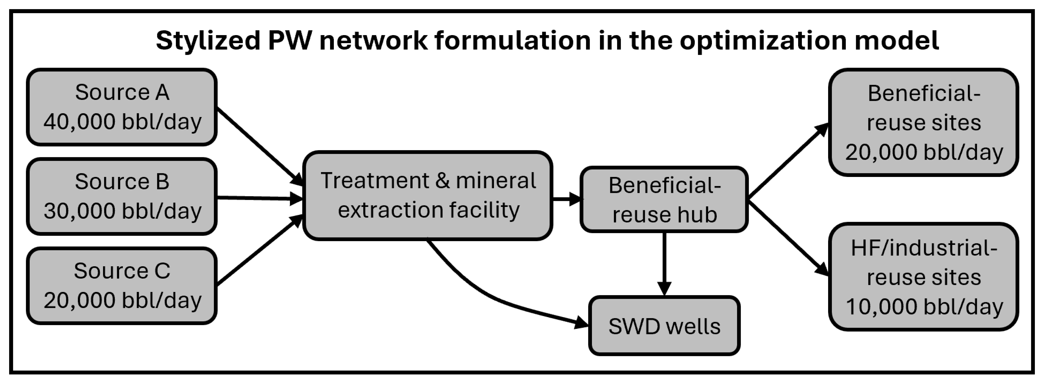
Table 5.
Key optimization variables and parameters.
3.5.2. Parameterization of Uncertainty Inputs
Table 6 lists the sampled inputs used in the screening-level Monte Carlo analysis; the TEA equations define the calculation structure, while Table 6 defines which inputs are varied. Uniform distributions are used when only lower and upper bounds are defensible and no single most-likely value can be justified at the screening stage. Triangular distributions are used when three screening-level quantities can be justified: a lower bound, a most-likely value (mode), and an upper bound. Accordingly, the “Mode/Mean” column in Table 6 reports the mode for triangular distributions and the arithmetic mean for uniform distributions. In other words, the triangular form represents bounded screening uncertainty with a preferred central estimate, whereas the uniform form is used when only a bounded range can be defended.
Table 6.
Techno-economic analysis (TEA) and Monte Carlo input assumptions used to compute screening-level lithium revenue and net advantage distributions.
The Monte Carlo analysis varies CLi, PLCE, ηDLE, preuse, cCAPEX,ann, cOPEX, cSWD, ctrans, xcap,retrofit, χcap,greenfield, χop,retrofit, and χop,greenfield, while discount rate r and project life N are held fixed for this screening study.
Rationale for Min/Central/Max of Table 6: This study is screening-level, so uncertain inputs are represented as simple distributions for Monte Carlo propagation. We use triangular distributions when the literature/pilot data suggest a plausible low value, a most-likely (central) value, and a plausible high value; we use uniform distributions when only bounds are defensible. The min/central/max values are taken from the cited source tables when available (chemistry percentiles, pilot windows, and published ranges); otherwise, they are stated as screening assumptions for sensitivity testing.
Brine chemistry (Li concentration). For Permian produced water, the Li range (uniform: 8–22 mg/L) is taken directly from the TxPWC chemistry screening percentiles and brackets Delaware-to-Midland variability; the reported mean (15 mg/L) is the midpoint used as a representative central value. For comparative benchmark brines, Smackover (uniform: 100–300 mg/L) and Salton Sea geothermal brines (uniform: 200–400 mg/L) follow the representative ranges summarized in Table 1.
Lithium value and recovery. LCE price is sampled as a triangular distribution (10–20–35 $/kg) to represent low/base/high commodity price scenarios; this same price grid logic is used in the break-even sensitivity table. DLE recovery efficiency is sampled uniformly (0.5–0.9) to reflect reported variability across DLE technologies and feed chemistries; pathway feasibility is additionally enforced by the chemistry-dependent feasibility indicator IKfeas(C).
Water value and cost terms. Reuse net value preuse, SWD fee CSWD, and transport/handling cost Ctrans are treated as triangular low/most-likely/high values because they are strongly site- and contract-dependent. Where possible, “typical” values are aligned with the order-of-magnitude Permian recycling vs. SWD costs cited in Section 2.1.3; higher-cost tails represent constrained-disposal or long-haul logistics regimes.
CAPEX/OPEX intensities and scenario multipliers. Annualized CAPEX intensity CCAPEX,ann and OPEX intensity COPEX are sampled as triangular distributions to capture screening uncertainty in technology choice, scaling, energy/chemical consumption, and installation context. Capital is annualized using the capital recovery factor (CRF) defined in Equation (8) with fixed r and project life N. Retrofit/greenfield multipliers (χ terms) are sampled uniformly to represent plausible ranges for integrating into existing infrastructure versus stand-alone deployment.
3.5.3. Objective Functions
We solve a tri-objective problem that (i) maximizes project net present value (NPV), (ii) minimizes the total volume routed to disposal sinks, and (iii) minimizes the injection-risk indicator R. The economic objective is based on discounted net cashflow over the project life and includes revenues from mineral products, avoided costs associated with SWD and freshwater purchases, and, where applicable, PRO energy credits [2,13,14]. The SWD objective is defined as the total produced-water volume routed to disposal sinks. The risk objective is represented by the injection-risk indicator R, aggregated over disposal hubs [4,5,9]. In practice, the PARETO frontier is generated using a weighted-sum or ε-constraint approach, allowing stakeholders to explore trade-offs among economic performance, disposal dependence, and relative injection risk [84]. More broadly, the framework is intended to reflect environmental trade-offs associated with produced-water routing, treatment, and disposal; however, in the present study these trade-offs are represented only through the injection-risk indicator R. Explicit carbon or life-cycle emissions metrics are not included and are left for future work.
3.5.4. Mass Balance and Capacity Constraints
The constraints enforce the physical and operational rules of the allocation network. In plain terms, the model decides what fraction of produced water from each source is (i) routed to candidate facilities for treatment and/or mineral recovery, (ii) delivered to each beneficial use sink, and (iii) sent to SWD either directly (bypass) or as residual brine after treatment. Conservation of mass is enforced at every node (all inflows are allocated to outgoing routes), facility flows cannot exceed installed capacity, and beneficial use deliveries are allowed only when predicted treated-water quality meets fit-for-purpose thresholds (e.g., TDS limits for discharge/recharge). When treatment capacity is insufficient, the model allows bypass routing to SWD to maintain feasibility [1,17]. Mass balance requires that all PW at each production node is allocated: ∑j xij = Qi for all i. Facility balance requires ∑k zjk = ∑i xij for all j. Capacity constraints are enforced as ∑i xij ≤ Capj yj for all j. Additional constraints represent end-use quality thresholds (e.g., maximum TDS for discharge/recharge), brine concentration limits, and minimum bypass volumes for SWD when treatment capacity is insufficient [1,15].
We enforce feasibility using five constraint groups (Equations (11)–(17)): (i) mass balance at sources and facilities (all inflow must be allocated), (ii) facility capacity limits (no unit can process more than its rated throughput), (iii) end-use demand/uptake caps (reuse cannot exceed sector demand or permitted capacity), (iv) fit-for-purpose quality constraints (predicted treated-water quality must meet the limit for each reuse class), and (v) injection operating limits (SWD volumes and pressure/ramp-rate limits constrain disposal routing). The equations below implement these rules. To ensure feasibility across end uses and injection operations, we impose the following constraints (indices and symbols are defined in Table 5).
Production node mass balance: Volume portions of PW are routed to a treatment facility or to SWD.
Facility mass balance: Inflow equals allocation to end uses plus residual routed to SWD.
Demand/uptake limits: Beneficial reuse is capped by sector-specific demand or permitted capacity.
Fit-for-purpose quality constraints: Surrogate models predict treated-water qualities (e.g., TDS, NH3-N, hardness), which must satisfy end-use limits L{u,m}. Here, f{m,j}(·) is the surrogate-predicted post-treatment value of constituent m at facility j as a function of influent chemistry Cj; θj denotes fixed surrogate parameters specified from screening parameter ranges and pilot-informed bounds (not decision variables). L{u,m} is the allowable limit for constituent m for end use u.
Throughput constraints: Each candidate facility has a capacity Capj (or scenario-dependent capacity window based on pilot performance).
Injection constraints: Total SWD is limited by available injection capacity CapSWD and operational pressure limit Pmax.
The screening-level injection-risk indicator R is appropriate here because the optimization requires a risk term (Equation (18)) that is (i) directionally consistently (higher injection intensity ⇒ higher risk), (ii) comparable across many scenarios, and (iii) computable from the same data typically available at the screening stage (volumes, routing, simple pressure/rate surrogates, and siting context). Accordingly, the composite structure in (16) intentionally aggregates normalized hazard-indicator functions—capturing induced seismicity and well-integrity/blowout tendencies—together with a disposal intensity penalty. This makes R appropriate for portfolio screening and trade-off exploration (PARETO ranking), while explicitly acknowledging that site-specific forecasting would require detailed geomechanics, fault models, and operational histories.
We therefore interpretate R as a normalized composite indicator in (16) that remains monotonic with injection intensity and siting sensitivity factors, ensuring R remains comparable across scenarios and suitable for multi-objective trade-off analysis at the screening stage. The weighting terms are tunable to local regulatory thresholds and basin-specific susceptibility.
Risk constraints can be imposed by bounding rate ramps (ΔQmax) and a hazard proxy Risk(·) (fault proximity and injection conditions) can be enforced below a threshold Riskmax or treated as the third objective in the PARETO set. In Equation (18), Iseis(·) and Iblow(·) are normalized hazard-indicator functions (increasing in injection rate and pressure) representing induced seismicity and well-integrity/blowout risk, respectively; wseis and wblow weight their relative importance. λSWD penalizes the fraction of total PW routed to SWD (QSWD/QPW), and Riskmax is an upper bound (or target) on the composite risk indicator.
In practice, nonlinear surrogate outputs and risk proxies can be (i) approximated with piecewise linear surrogates, (ii) handled via a sequential mixed-integer linear program, or (iii) optimized with derivative-free multi-objective methods while preserving the same constraint structure.
3.5.5. Uncertainty Treatment
Key uncertainties include lithium concentration, LCE price, DLE recovery efficiency, SWD fee, reuse value, transport cost, and cost intensities. Distribution and correlation assumptions: Where the literature or project data provide only credible lower/upper bounds, we use uniform distributions to avoid implying a most-likely value that is not supported. Where a central estimate is defensible (e.g., from historical averages or reported pilot medians), we use triangular distributions to reflect a most-likely value with bounded tails. Strictly positive multiplicative factors (e.g., CAPEX/OPEX adjustment multipliers) can be represented as lognormal when variability is better interpreted in percentage terms. Baseline sampling assumes independence among uncertain inputs for screening-level analysis; to test robustness, we additionally evaluate sensitivity cases with rank correlations among key drivers (e.g., commodity prices, electricity cost, and operating cost multipliers) to ensure conclusions do not depend on a zero-correlation assumption (we will include correlated sensitivity as future work). We propagate these uncertainties with Monte Carlo sampling: each realization draws an input vector from the distributions summarized in Table 6 and evaluates the economic model in Equations (6)–(10). Retrofit (primary) and greenfield (sensitivity) cases are distinguished by applying the CAPEX and OPEX adjustment factors χcap,s and χop,s in Equations (1) and (2). The resulting NetAdv ($/m3) distributions are reported and summarized as a worked example in Section 4.4.
The optimization can be implemented as a mixed-integer linear program when surrogate outputs are pre-computed coefficients, and nonlinearities are linearized via piecewise approximations. Open-source (CBC) or commercial solvers (Gurobi/CPLEX) can be used depending on problem size. A weight sweep or ε-constraint loop produces the PARETO set, which is then visualized in the decision interface for interactive exploration [6,84].
Algorithm 1 emphasizes that the surrogate layer decouples expensive mechanistic simulation from portfolio screening, enabling fast evaluation of many chemistry/price scenarios while preserving constraints from fit-for-purpose water quality and injection risk management. Economic and cost uncertainty distributions (SWD fees, transport costs, commodity prices, and retrofit/greenfield multipliers) are summarized in Table 6 and are propagated via Monte Carlo alongside surrogate output sampling.
| Algorithm 1 Surrogate-assisted multi-objective decision workflow for produced-water portfolio optimization under uncertainty |
| 1. Input: PW volumes Qi, chemistry vectors Ci, candidate pathways p, demand caps Du, and price/cost distributions. 2. Feature engineering: Compute geochemical features (e.g., ionic strength, scaling indices) and normalize inputs for surrogate models. 3. Surrogate evaluation: For each pathway p, predict (a) recovery ηj,p(Ci), (b) treated-water quality ,p(Ci), and (c) unit costs/energy from trained machine learning surrogates calibrated to pilot/field data. 4. Scenario sampling: Draw uncertainty scenarios ω (Monte Carlo) or simulate regime sequences (Markov states) for {Pj, cSWD, celec, …}. 5. Optimization: Solve the tri-objective allocation problem (NPV, SWD volume, risk) via ε-constraint or weighted-sum sweeps to generate the PARETO frontier. 6. Post-processing: Report recommended allocations by end use (municipal, irrigation, industrial, recharge, and discharge), mineral product slate, and key sensitivities; compute robustness metrics (e.g., probability NPV > 0, worst-case SWD). 7. Update loop: As new sampling/pilot data arrive, retrain surrogates, and re-optimize to refine the recommended portfolio. |
3.6. Case Study Configuration
For the Permian Basin, we addressed the Delaware and Midland Basins separately because their chemistry percentiles differ substantially (Table 2), leading to different treatment costs and mineral recovery potential. For Smackover and Salton Sea, the framework is used to illustrate how chemistry-rich brines may shift the PARETO frontier toward mineral recovery, provided that environmental safeguards, permitting, and brine management plans are addressed [8,12,82,83]. All case studies are intended for comparative screening and sensitivity testing; site-specific feasibility would require facility-level operating data, permitting constraints, and detailed brine management/waste characterization.
3.6.1. Comparative Brine Systems: Smackover and Salton Sea
To generalize beyond the Permian Basin, we position the Smackover Formation brines (southern Arkansas) and the Salton Sea geothermal brines (southern California) as comparative case studies [8,12,82,83]. These systems span a wide range of salinity, temperature, and trace-element assemblages, and they provide real-world analogs for “high-Li” brines where mineral recovery has advanced toward commercial pilots. Within our workflow, these case studies are used to (i) benchmark chemistry-driven yields, (ii) compare TEA break-even conditions across brine types, and (iii) demonstrate the transferability of the surrogate decision engine. Smackover Formation and Salton Sea geothermal fluids are introduced in Section 2.1.3; here, we use them only to parameterize comparative scenarios for the case study analyses.
3.6.2. Scenario Families
We organize scenario exploration into families that reflect plausible regulatory and market futures: (S1) baseline SWD-dominant management; (S2) reuse expansion with fixed treatment capacity; (S3) disposal constraints via rate caps or seismicity-triggered shutdowns; (S4) mineral-recovery incentives (high price/tax credits) and learning curves; and (S5) combined portfolios that include PRO energy credits and nutrient recovery where relevant [9,13,14,81]. Unless explicitly stated otherwise, the ammonia-recovery module is inactive in the base-case Permian scenarios and is activated only in pathway-specific sensitivity runs where ammonia concentration and nitrogen-management assumptions are provided.
Each scenario family is evaluated across uncertainty realizations to quantify robustness rather than single-point optimality [84].
4. Results
4.1. Chemistry Screening for the Delaware and Midland Basins
4.1.1. Disposal Reliance and Cost Exposure
Across Texas, PW volumes have increased with unconventional development, and the Permian Basin dominates statewide totals [1,2]. Even with substantial HF reuse, operators remain exposed to SWD availability, pricing, and regulatory limits [1,9]. In our framework, this exposure is represented as an avoided-cost credit when disposal is displaced (reused or valorized), and as an explicit risk penalty when injection volumes concentrate near high-susceptibility areas [4,5,9].
4.1.2. Chemistry Heterogeneity and Its Engineering Consequences
The chemistry percentiles summarized below are important not only for mineral-recovery potential (e.g., Li, B, and Sr) but also for treatment operability [1,7]. High divalent-ion content and scaling tendency typically imply higher pretreatment requirements and shorter membrane/sorbent lifetimes, increasing OPEX and limiting feasible recovery [15]. Conversely, brines with favorable Li/TDS ratios can support higher-value recovery even when absolute salinity is high, if scaling and organics are managed effectively [7].
The TxPWC reported chemistry percentiles for 7024 PW samples from the Delaware and Midland Basins (January 2022–January 2024) [1]. Table 2 summarizes the reported percentiles and highlights three key implications: (i) Midland Basin brines exhibit higher TDS percentiles than Delaware Basin brines, which can increase desalination energy demand and scaling risk; (ii) divalent cations (Ca, Ba, and Sr) and sulfate promote scale formation, which can dictate pretreatment requirements; and (iii) lithium and other trace constituents provide a rationale for screening mineral recovery as an SWD cost-offset in specific subareas.
4.2. TxPWC Pilots and Representative Performance Windows
The TxPWC documented multiple pilot-scale PW treatment demonstrations across the Permian Basin, spanning thermal desalination, advanced thermal processes, and reverse-osmosis variants [1]. Table 3 summarizes these pilots as representative performance windows that can be used to calibrate surrogate yield and cost functions. In practice, pilot-specific data (energy intensity, chemical dosing, recovery fraction, brine management, and downtime) are required to build bankable TEA models; however, the pilots provide a defensible starting point for scenario screening.
4.3. Surrogate Decision Engine and Allocation Outputs
To support “design matrix” planning, the model can also be run as a stress test in which disposal options are progressively restricted (rate caps and shut-ins triggered by seismicity thresholds) [9]. In these runs, the value of treatment and mineral recovery is quantified not only as profit but as operational resilience, i.e., the ability to maintain production while complying with evolving injection limits. Figure 3 and Figure 4 are used here to contextualize how the optimization framework translates chemistry, routing, and facility choices into basin-level allocation outcomes. The decision engine and network formulation introduced in the Results section were applied here to generate basin-specific allocation portfolios under chemistry, cost, capacity, and risk constraints.
4.4. Illustrative TEA Sensitivities for Lithium and Avoided Disposal
Figure 5 and Figure 6 are generated directly from the economic relations in Equations (6)–(10). Figure 5 evaluates the lithium revenue term by varying CLi and PLCE while holding other parameters at representative values. Figure 6 propagates uncertainty by sampling the TEA inputs and scenario multipliers listed in Table 6 and computing NetAdv ($/m3) via Equation (10) for both retrofit (primary) and greenfield (sensitivity) infrastructure assumptions. Table 7 lists the lithium concentration required for the gross lithium revenue to cover avoided SWD costs for different LCE prices. Table 8 lists the volumetric assumptions used to generate the results of Figure 6.
Figure 5.
Screening-level gross annual lithium revenue computed from Equations (4) and (6)–(10) as a function of lithium concentration (mg/L) and lithium carbonate equivalent (LCE) price. Gross lithium revenue RevLi scales linearly with concentration and price for a fixed treated fraction QDLE/QPW.
Figure 6.
Monte Carlo distribution of net advantage (Equation (10)) computed from Equations (6)–(10) for retrofit (primary) and greenfield (sensitivity) scenarios, using sampled input ranges and distributions in Table 6 for three representative brine systems. Boxes show the median and interquartile range; whiskers denote the 5th–95th percentiles.
Table 7.
Screening-level decision boundary for lithium: break-even Li concentration (mg/L) such that gross Li revenue equals avoided SWD cost (excludes CAPEX/OPEX; assumes DLE recovery η = 0.7).
Table 8.
Worked example portfolio outcomes for three representative brine systems (Permian, Smackover, Salton Sea). Reported values are the median across Monte Carlo samples generated from the input distributions in Table 6 and evaluated using Equations (6)–(10); avoided SWD volume is computed from the nominal throughput QPW.
4.5. Comparative Case Study Benchmarks: Smackover and Salton Sea
The Smackover and Salton Sea brines provide useful benchmarks for interpreting Permian screening results [8,12,82,83]. First, they demonstrate that commercially relevant lithium recovery is possible when chemistry supports high selectivity and when infrastructure (power, brine handling, and product logistics) is available [82,83]. Second, they highlight that the “best” recovery pathway depends on brine-specific constraints: geothermal brines can offer elevated temperatures that reduce thermal penalties but may impose unique corrosion and scaling challenges; formation brines, such as the Smackover brines, may exhibit more stable compositions but require different pretreatment and concentrate management strategies [7,8]. In the proposed workflow, these benchmarks help bind plausible recovery factors and unit costs, reducing the risk of over-optimistic TEA results when only limited Permian pilot data are available.
A key implication is that transfer learning is feasible: surrogate models trained on one brine system can be adapted to another via chemistry-aware feature engineering and limited new pilot data, allowing rapid evaluation of whether a Permian sub-region is more “Smackover-like” (mineral-driven) or more “reuse-driven” (treatment and allocation dominate) [8,16,17].
5. Discussion
5.1. When Can Mineral Recovery Offset SWD Costs?
Mineral recovery is most attractive when three conditions align: (i) sufficiently high target-ion concentrations in the source brine, (ii) process selectivity that limits reagent and brine management costs, and (iii) market prices that justify capital deployment. Smackover brines and Salton Sea geothermal brines are prominent U.S. examples where lithium concentrations and resource assessments support continued evaluation of commercial recovery [8,12,82,83]. In the Permian Basin, lithium concentrations are typically lower than these dedicated resource brines, but the TxPWC’s dataset indicates that lithium is present and may justify selective recovery in targeted subareas, especially when combined with avoided SWD costs and co-product strategies [1,7].
5.2. Design Matrix for Reducing Blowout and Seismicity Risk
A key advantage of reducing SWD volumes is the potential reduction in injection-driven hazards. Based on the induced seismicity literature and the Permian blowout case study [3,4,5], a practical risk-reduction matrix for operators (Table 9) includes: (i) prioritizing reuse and valorization in or near seismic response areas; (ii) limiting injection rates and maintaining conservative pressure margins; (iii) increasing real-time monitoring of injection pressures and local seismicity; (iv) optimizing well placement and completion intervals to avoid basement-connected faults; and (v) developing contingency plans to rapidly reroute water to treatment or alternative disposal when regulatory triggers are met [9]. Within the proposed framework, these measures can be encoded as constraints or penalties so that the optimizer preferentially selects portfolios that lower both SWD costs and hazard indicators.
Table 9.
Design matrix of operational levers to reduce SWD-related blowout and induced seismicity hazards (qualitative).
5.3. Implementation Pathway and Data Needs
To transition from screening to deployment, three data layers are required: (i) brine characterization (major ions, trace metals/REEs, organics, and ammonia) and temporal variability; (ii) process performance data for treatment and recovery units (including brine management and waste handling); and (iii) basin-specific constraints (underground injection permitting, reuse/discharge regulations, and local SWD pricing). The United States Department of Energy emphasized that open data resources and decision-support tools, e.g., its Constituent Data Replacement Tool and PARETO, can accelerate the integration of these layers [6,16,17]. In parallel, early TEA should be paired with environmental and health safeguards to ensure that beneficial use does not shift risk from deep disposal to surface exposure [15]. Classical PW reuse considerations are summarized by Veil [10], while chemical disclosure resources for stimulation additives can be accessed via FracFocus [24].
5.4. Regulatory, Monitoring, and Stakeholder Considerations
PW valorization decisions intersect with regulatory frameworks for underground injection (Class II), surface discharge permits, and water quality standards for reuse and recharge [11]. A pragmatic deployment strategy is to align early projects with pathways that have the clearest permitting routes (e.g., reuse within the oilfield or industrial reuse with defined treatment objectives), while collecting the monitoring data needed to expand into higher-barrier pathways (recharge or discharge) [42]. For injection risk, existing seismic response plans and traffic light approaches provide a governance scaffold: the surrogate engine can be used to pre-compute contingency allocations that are triggered when injection rate reductions are required [9,40].
5.5. Optional Nutrient Recovery Module (Ammonia)
Ammonia is treated in this study as an optional, chemistry-triggered module rather than as a driver of the reported base-case Permian results. Unless otherwise stated, the base-case scenarios and headline results presented in Section 4 and Section 5 do not activate the ammonia-recovery module. The module is only considered when ammonia concentration, treatment-train compatibility, and nitrogen-management requirements are explicitly specified for a given pathway [80]. In those cases, ammonia enters the TEA as a conditional revenue or avoided-cost term. Because these pathway-specific ammonia inputs are not available consistently across the basin-wide dataset used here, ammonia recovery is not used as a primary result driver; lithium and REE recovery remain the principal mineral-offset mechanisms [7,8,12,82,83]. Reproducible activation of the ammonia module requires three user-specified inputs: influent ammonia concentration, recovery/removal efficiency, and ammonia-credit or avoided-treatment value.
5.6. Limitations and Next Steps
The framework is designed for decision support rather than as a substitute for site-specific engineering. Key limitations include: (i) data sparsity for trace elements and organics in many PW datasets, (ii) uncertainty in long-term product pricing and offtake contracts, and (iii) the need to reconcile model outputs with local infrastructure and community constraints. Future work should focus on: (i) expanding open chemistry datasets with consistent quality assurance and quality control, (ii) calibrating surrogates to pilot-scale mass balances whilst utilizing field measurements, (iii) validating risk indicators against observed injection responses, and (iv) integrating dynamic routing that reflects temporal variability in PW volumes and seismicity triggers mainly in the Permian Basin in high-SWD counties such as Martin and Culberson [1,2,9,15,16,17]. We suggest the need to consider net volumes of PW (available after use in HF, e.g., about 2,385,000 m3/day in the Permian) in a future quantitative framework that allocates the available water to different potential uses while accounting for available disposal capacity and induced seismicity risk. The qualitative framework suggested in our manuscript (assessing water quality) can be used to help choose/justify an optimal location for treatment if coupled with previous spatiotemporal work [2], and would require adequate forecasts of production and water-use needs/demands.
We have developed geospatial maps of mineral distribution based on water-quality data of PW sampled from unconventional wells in the Permian Basin between 2013 and 2025 (Figure A2): we collected the data by surveying operators and service companies and by downloading public data from the U.S. Geological Survey [86]. We suggest future work to utilize such geospatial data for water-use optimization.
6. Conclusions
PW management can be framed as a portfolio optimization problem under chemistry, market, and regulatory uncertainty. By combining chemistry-informed surrogate yield functions with TEA and PARETO-based network optimization, the proposed workflow identifies when treatment, reuse, and critical mineral recovery can reduce SWD volumes and potentially offset disposal costs. Incorporating injection-related hazard indicators (seismicity and blowout risk) as explicit decision criteria further aligns economic decision-making with societal risk reduction. The tri-objective formulation (expected NPV, SWD volume, and an injection-risk indicator R) generates PARETO-efficient portfolios that make trade-offs transparent. Across uncertainty scenarios, results indicate that (i) avoided SWD cost and operational feasibility dominate near-term economics in most Permian chemistry windows, (ii) mineral recovery can act as a conditional cost offset but is strongly sensitive to brine chemistry and market conditions, and (iii) risk-reducing allocations that shift volumes away from higher-sensitivity disposal options can be achieved with measurable economic trade-offs. For decision-makers, the resulting PARETO frontiers provide a practical basis to compare portfolios that prioritize profitability versus those that prioritize SWD reduction and injection-risk reduction. Future work should (i) calibrate and validate surrogate models with site-specific pilot data and expanded trace-element datasets (including REEs), (ii) strengthen the injection-risk indicator R by incorporating local injection rate/pressure limits, seismic response datasets, and geospatial sensitivity weighting, (iii) extend the optimization to a multi-period (dynamic) setting to capture evolving production, infrastructure buildout, and regulatory constraints, and (iv) integrate life-cycle metrics (energy use, emissions, and chemical intensity) so economic and environmental trade-offs can be assessed consistently. Operators should interpret mineral valorization revenue as scenario-dependent and evaluate it alongside avoided SWD and fit-for-purpose reuse benefits rather than as a guaranteed primary driver.
Author Contributions
Conceptualization, A.T. and E.B.; methodology, A.T.; software, A.T.; validation, A.T.; formal analysis, A.T.; investigation, A.T., E.B., M.W. and S.P.; resources, E.B., M.W. and S.P.; data curation, A.T.; writing—original draft preparation, A.T. and E.B.; writing—review and editing, E.B., M.W. and S.P.; visualization, A.T.; supervision, M.W.; project administration, M.W.; All authors have read and agreed to the published version of the manuscript.
Funding
This research received no external funding.
Data Availability Statement
The original contributions presented in this study are included in the article. All processed inputs required to reproduce the analysis, including produced-water chemistry percentiles, pilot performance windows, and techno-economic/Monte Carlo input distributions, are reported in the manuscript tables. The underlying source data were derived from publicly available reports and publications cited in the References. Further inquiries can be directed to the corresponding author.
Acknowledgments
The authors acknowledge the Texas Produced Water Consortium for publicly reporting the basin chemistry percentiles and pilot summaries used for this manuscript.
Conflicts of Interest
The authors declare no conflicts of interest.
Nomenclature
| Acronym | Description |
| PW | Produced Water |
| CAPEX | Capital Expenditure |
| CRF | Capital Recovery Factor |
| DLE | Direct Lithium Extraction |
| HF | Hydraulic Fracturing |
| LCE | Lithium Carbonate Equivalent |
| NPV | Net Present Value |
| OPEX | Operating Expenses |
| PARETO | The US Department of Energy: The Produced Water Application for Beneficial Reuse, Environmental Impact and Treatment Optimization |
| PRO | Pressure-Retarded Osmosis |
| REEs | Rare Earth Elements |
| SWD | Saltwater Disposal |
| TDS | Total Dissolved Solids |
| TEA | Techno-Economic Analysis |
| TxPWC | Texas Produced Water Consortium |
Appendix A
Figure A1.
East-to-west geologic cross sections A-A′ through the Permian Basin: highlighted in bold red font and underlined is the Wolfcamp A formation, which contour is shown in Figure 1. We edited the source figure for proper legibility: the figure is sourced from a report issued by the U.S. Energy Information Administration in 2020 [87]. The U.S. Energy Information Administration determined depth and thickness of each formation based on logs of various wells with different well numbers, as indicated in this figure.
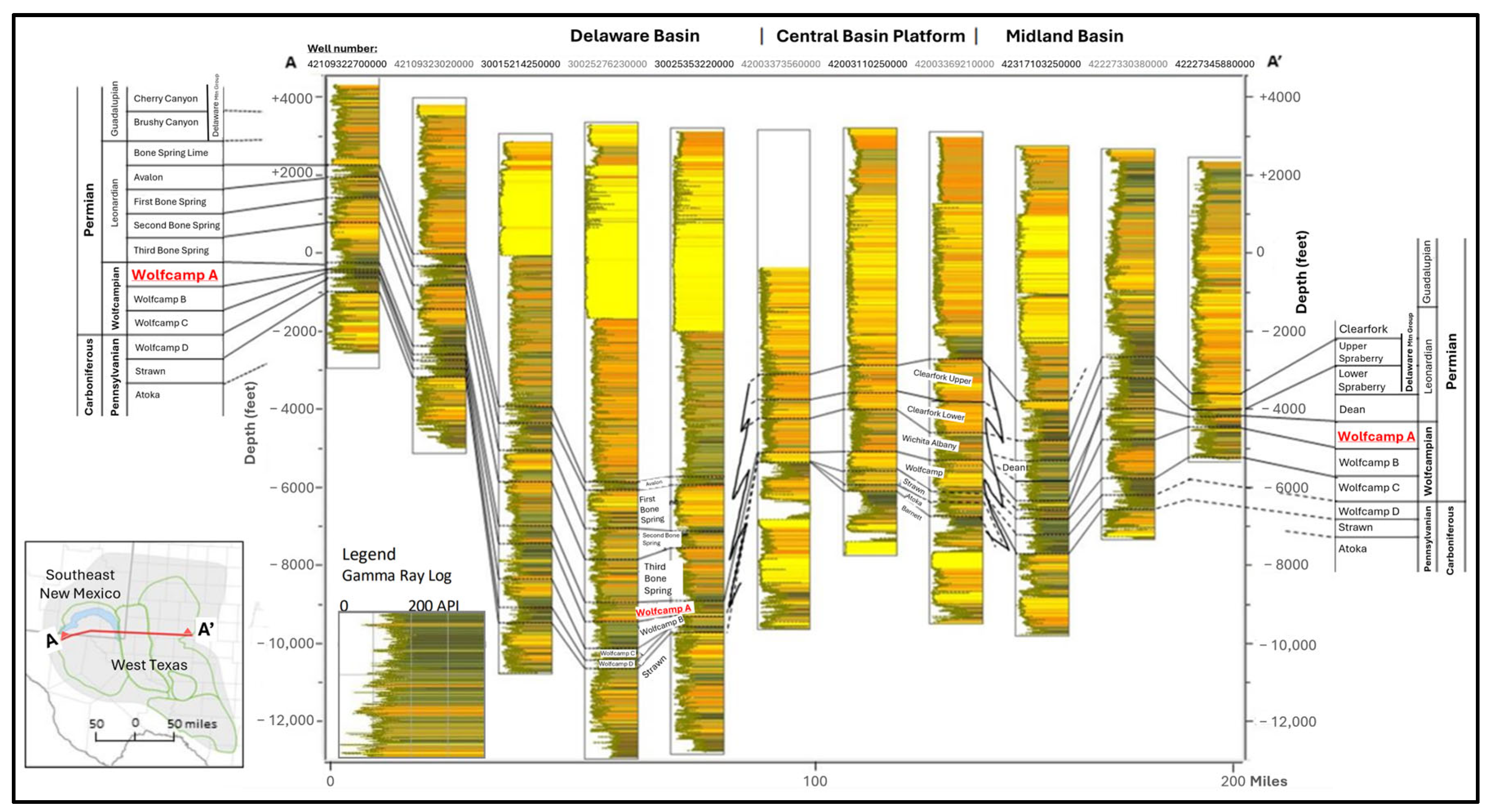
Figure A2.
Geospatial count and mineral concentrations of produced-water samples collected from unconventional formations in the Permian Basin between 2013 and 2025: (a) distribution of sample count, (b) distribution of median total dissolved solids (TDS) in mg/L, (c) distribution of median lithium concentration in mg/L, (d) distribution of median boron concentration in mg/L. The dataset consists of data publicly available through the U.S. Geological Survey [86], and of data provided to our research team by chemical companies and oil-and-gas operators, herein credited [88,89,90,91,92,93,94,95].
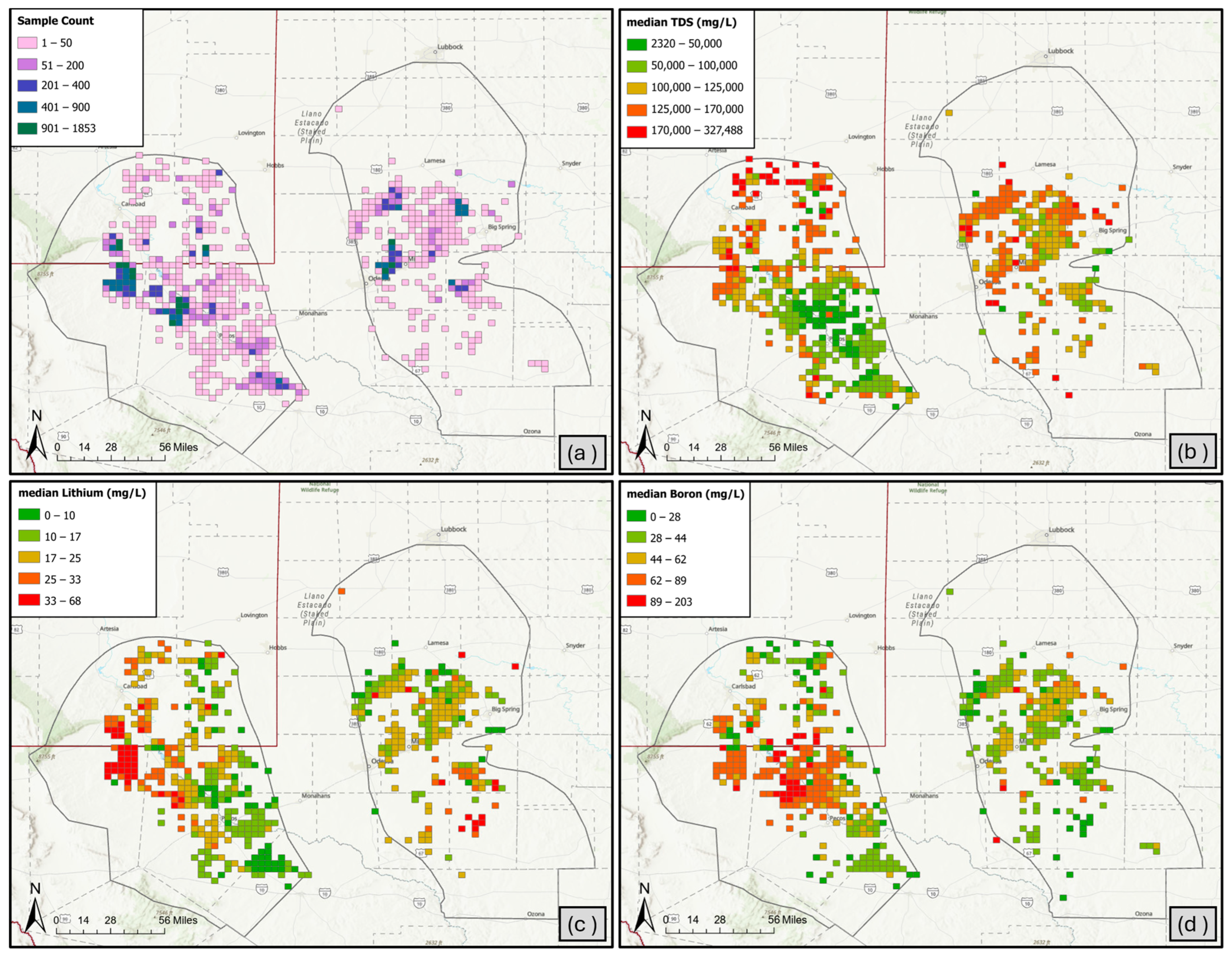
References
- Smith, R.; Mauldin, W.; Bernard, E.; Jagadish, K.; Rao, B.; Reible, D.; Walker, S.; Watson, M.; Williams, R.; Samper, B.; et al. Beneficial Use of Produced Water in Texas; Texas Produced Water Consortium Report to the Texas Legislature 2024; Texas Produced Water Consortium: Lubbock, TX, USA, 2024; Available online: https://www.depts.ttu.edu/research/tx-water-consortium/2024-report.php (accessed on 29 December 2025).
- Bechara, E.; Watson, M.; Arbad, N. Unlocking Sustainability: Transforming Tight-Oil Produced Water into a Lifeline for West Texas. Environ. Process. 2024, 11, 26. [Google Scholar] [CrossRef] [Scilit]
- Karanam, V.; Lu, Z.; Kim, J. Investigation of Oil Well Blowouts Triggered by Wastewater Injection in the Permian Basin, USA. Geophys. Res. Lett. 2024, 51, e2024GL109435. [Google Scholar] [CrossRef] [Scilit]
- U.S. Geological Survey. Induced Earthquakes; U.S. Geological Survey: Reston, VA, USA, 2025. Available online: https://www.usgs.gov/programs/earthquake-hazards/science/induced-earthquakes (accessed on 29 December 2025).
- Weingarten, M.; Ge, S.; Godt, J.W.; Bekins, B.A.; Rubinstein, J.L. High-rate injection is associated with the increase in U.S. mid-continent seismicity. Science 2015, 348, 1336–1340. [Google Scholar] [CrossRef] [Scilit] [PubMed]
- U.S. Department of Energy. Fact Sheet: Produced Water from Oil and Gas Development and Critical Minerals; U.S. Department of Energy: Washington, DC, USA, 2024. Available online: https://www.energy.gov/hgeo/articles/fact-sheet-produced-water-oil-and-gas-development-and-critical-minerals (accessed on 29 December 2025).
- Murphy, O.; Haji, M.N. A review of technologies for direct lithium extraction from low Li+ concentration aqueous solutions. Front. Chem. Eng. 2022, 4, 1008680. [Google Scholar] [CrossRef] [Scilit]
- Knierim, K.J.; Blondes, M.S.; Masterson, A.; Freeman, P.; McDevitt, B.; Herzberg, A.; Li, P.; Mills, C.; Doolan, C.; Jubb, A.M.; et al. Evaluation of the lithium resource in the Smackover Formation brines of southern Arkansas using machine learning. Sci. Adv. 2024, 10, eadp8149. [Google Scholar] [CrossRef] [Scilit]
- Railroad Commission of Texas. Seismicity Response; Railroad Commission of Texas: Austin, TX, USA, 2025. Available online: https://www.rrc.texas.gov/oil-and-gas/applications-and-permits/injection-storage-permits/oil-and-gas-waste-disposal/injection-disposal-permit-procedures/seismicity-review/seismicity-response/ (accessed on 29 December 2025).
- Veil, J.; Puder, M.; Elcock, D.; Redweik, R. A White Paper Describing Produced Water from Production of Crude Oil, Natural Gas, and Coal Bed Methane; National Energy Technology Laboratory: Morgantown, WV, USA, 2004.
- U.S. Environmental Protection Agency. Class II Oil and Gas Related Injection Wells; U.S. Environmental Protection Agency: Washington, DC, USA, 2025. Available online: https://www.epa.gov/uic/class-ii-oil-and-gas-related-injection-wells (accessed on 29 December 2025).
- Knierim, K.J.; Masterson, A.L.; Freeman, P.A.; McDevitt, B.; Herzberg, A.H.; Li, P.; Mills, C.; Doolan, C.; Jubb, A.M.; Ausbrooks, S.M.; et al. Lithium Resource in the Smackover Formation Brines of Southern Arkansas; U.S. Geological Survey: Reston, VA, USA, 2024. [CrossRef] [Scilit]
- Yip, N.Y.; Elimelech, M. Thermodynamic and Energy Efficiency Analysis of Power Generation from Natural Salinity Gradients by Pressure Retarded Osmosis. Environ. Sci. Technol. 2012, 46, 5230–5239. [Google Scholar] [CrossRef] [Scilit]
- Gonzales, R.R.; Abdel-Wahab, A.; Adham, S.; Han, D.S.; Phuntsho, S.; Suwaileh, W.; Hilal, N.; Shon, H.K. Salinity gradient energy generation by pressure retarded osmosis: A review. Desalination 2021, 500, 114841. [Google Scholar] [CrossRef] [Scilit]
- Fakhru’l-Razi, A.; Pendashteh, A.; Abdullah, L.C.; Biak, D.R.A.; Madaeni, S.S.; Abidin, Z.Z. Review of technologies for oil and gas produced water treatment. J. Hazard. Mater. 2009, 170, 530–551. [Google Scholar] [CrossRef] [Scilit]
- Drouven, M.G.; Caldéron, A.J.; Zamarripa, M.A.; Beattie, K. PARETO: An open-source produced water optimization framework. Optim. Eng. 2023, 24, 2229–2249. [Google Scholar] [CrossRef] [Scilit]
- National Energy Technology Laboratory. Project PARETO—DOE’s Produced Water Optimization Initiative; National Energy Technology Laboratory: Pittsburgh, PA, USA, 2022. Available online: https://netl.doe.gov/ (accessed on 22 December 2025).
- ALL Consulting. U.S. Produced Water Volumes and Management Practices in 2021. Ground Water Protection Council 2022. Available online: https://www.gwpc.org/wp-content/uploads/2021/09/2021_Produced_Water_Volumes.pdf (accessed on 28 April 2024).
- International Energy Agency. World Energy Outlook Special Report 2016: Water-Energy Nexus; International Energy Agency: Paris, France, 2016. [Google Scholar]
- Eyitayo, S.I.; Watson, M.C.; Kolawole, O.; Xu, P.; Lawal, K.A.; Wigwe, M.E.; Giussani, A. Novel systematic approach for produced water volume quantification applicable for beneficial reuse. Environ. Sci. Adv. 2023, 2, 508–528. [Google Scholar] [CrossRef] [Scilit]
- Salem, F.; Thiemann, T. Produced Water from Oil and Gas Exploration—Problems, Solutions and Opportunities. J. Water Resour. Prot. 2022, 14, 142–185. [Google Scholar] [CrossRef]
- Enverus. PRISM, Enverus: Austin, TX, USA, 2025. Available online: https://www.enverus.com/solutions/energy-analytics/ep/prism/ (accessed on 19 December 2025).
- B3 Insight. Water Market Trends and Forecast Report; B3 Insight: Denver, CO, USA, 2024; Available online: https://www.b3insight.com/ (accessed on 3 September 2024).
- FracFocus. FracFocus—Data Download; FracFocus: Oklahoma City, OK, USA, 2025; Available online: https://fracfocus.org/data-download (accessed on 19 December 2025).
- Redman, A.D.; Key, T.; Koster van Groos, P.; Smith, A.; Sutherland, C.; Reddington, T.; Kung, M.; Davis, C.; Butler, J.; Hedgpeth, B.; et al. Integrated Assessment of Whole Effluent Toxicity Tests and Chemical Characterization of Treated Permian Basin Produced Water. ACS ES&T Water 2025, 5, 5275–5286. [Google Scholar] [CrossRef] [Scilit]
- Ariana, A.; Cozzarelli, I.; Danforth, C.; McDevitt, B.; Rosofsky, A.; Vorhees, D. Pathways for Potential Exposure to Onshore Oil and Gas Wastewater: What We Need to Know to Protect Human Health. Geohealth 2025, 9, e2024GH001263. [Google Scholar] [CrossRef] [Scilit]
- Chen, F.; Ma, Z.; Nasrabadi, H.; Chen, B.; Mehana, M.; Van Wijk, J. Reuse of Produced Water from the Petroleum Industry: Case Studies from the Intermountain-West Region, USA. Energy Fuels 2023, 37, 3672–3684. [Google Scholar] [CrossRef] [Scilit]
- Railroad Commission of Texas. Data Sets Available for Download; Railroad Commission of Texas: Austin, TX, USA, 2024. Available online: https://www.rrc.texas.gov/resource-center/research/data-sets-available-for-download/ (accessed on 20 November 2022).
- Oil Conservation Division. C-115 (Operator’s Monthly Report) Instructions; Energy, Minerals and Natural Resources Department: Santa Fe, NM, USA, 2023. Available online: https://www.emnrd.nm.gov/ocd/wp-content/uploads/sites/6/C115-INSTRUCTIONS.pdf (accessed on 19 December 2025).
- Warren, I. Techno-Economic Analysis of Lithium Extraction from Geothermal Brines; National Renewable Energy Laboratory: Golden, CO, USA, 2021. [CrossRef] [Scilit]
- Stringfellow, W.T.; Dobson, P.F. Technology for the Recovery of Lithium from Geothermal Brines. Energies 2021, 14, 6805. [Google Scholar] [CrossRef] [Scilit]
- O’Sullivan, J.; Araya, N.; Popineau, J.; Renaud, T.; Riffault, J.; O’Sullivan, M. Investigating Reinjection Strategies to Optimise Lithium Production from the Salton Sea Geothermal Field. In 49th Workshop on Geothermal Reservoir Engineering; Stanford University: Stanford, CA, USA, 2024; pp. 1–18. [Google Scholar]
- Kong, L.; Yan, G.; Hu, K.; Yu, Y.; Conte, N.; Mckenzie, K.R., Jr.; Wagner, M.J.; Boyes, S.G.; Chen, H.; Liu, C.; et al. Electro-driven direct lithium extraction from geothermal brines to generate battery-grade lithium hydroxide. Nat. Commun. 2025, 16, 806. [Google Scholar] [CrossRef] [Scilit]
- Dobson, P.; Araya, N.; Brounce, M.; Busse, M.; Camarillo, M.K.; English, L.; Humphreys, J.; Kalderon-Asael, B.; McKibben, M.; Millstein, D.; et al. Characterizing the Geothermal Lithium Resource at the Salton Sea; eScholarship Repository: Berkeley, CA, USA, 2023. [Google Scholar] [CrossRef] [Scilit]
- Busse, M.M.; Stokes-Draut, J.; Camarillo, M.K.; Millstein, D.; Slattery, M.; McKibben, M.; Dobson, P.; Stringfellow, W. Environmental Impact Assessment of Lithium Recovery from Geothermal Brines in the SS-KGRA: An Overview; Geothermal Resources Council Transactions; Geothermal Rising: Reno, Nevada, USA, 2023; Volume 47, pp. 192–200. [Google Scholar]
- Hewett, C. The Race to Extract Lithium Around the Salton Sea Area; Electrify News: Spicewood, TX, USA, 2024; Available online: https://electrifynews.com/news/batteries/the-race-to-extract-lithium-around-the-salton-sea-area/ (accessed on 23 December 2025).
- Helerea, E.; Calin, M.D.; Musuroi, C. Water Energy Nexus and Energy Transition—A Review. Energies 2023, 16, 1879. [Google Scholar] [CrossRef] [Scilit]
- Patton, P. Balancing Growth and Risk: Why Water Management Is the Permian Basin’s Biggest Challenge; The Way Ahead, Journal of Petroleum Technology; Society of Petroleum Engineers: Richardson, TX, USA, 2025; Available online: https://jpt.spe.org/twa/balancing-growth-and-risk-why-water-management-is-the-permian-basins-biggest-challenge/ (accessed on 23 December 2025).
- Hennings, P.H.; Young, M.H. The TexNet-CISR Collaboration and Steps Toward Understanding Induced Seismicity in Texas. In Recent Seismicity in the Southern Midcontinent, USA: Scientific, Regulatory, and Industry Responses; Kyle, E., Murray, K.E., Young, M.H., Buchanan, R., Eds.; Special Paper 559; The Geological Society of America: Boulder, CO, USA, 2023. [Google Scholar] [CrossRef] [Scilit]
- Railroad Commission of Texas. Notice to Oil and Gas Operators—Disposal Well Monitoring and Reporting Requirements in the Permian Basin; Railroad Commission of Texas: Austin, TX, USA, 2023. Available online: https://www.rrc.texas.gov/media/l1on5x0d/2023-nto-disposal-well-monitoring-reporting-requirements-in-the-permian-basin-2-6-2023.pdf (accessed on 20 July 2023).
- Rodriguez, A.Z.; Wang, H.; Hu, L.; Zhang, Y.; Xu, P. Treatment of Produced Water in the Permian Basin for Hydraulic Fracturing: Comparison of Different Coagulation Processes and Innovative Filter Media. Water 2020, 12, 770. [Google Scholar] [CrossRef] [Scilit]
- Smith, R.; Bernard, E.; Watson, M.; Reible, D.; Uddameri, V.; Rao, B.; Craig, R.; Castilleja, A.; Eyitayo, S.; Bechara, E.; et al. Beneficial Use of Produced Water in Texas: Challenges, Opportunities and the Path Forward; Texas Produced Water Consortium: Lubbock, TX, USA, 2022; Available online: https://www.depts.ttu.edu/research/tx-water-consortium/2022-report.php (accessed on 28 April 2024).
- Texas Water Development Board. 2022 State Water Plan: Water for Texas; Texas Water Development Board: Austin, TX, USA, 2022. Available online: www.twdb.texas.gov/waterplanning/swp/2022 (accessed on 15 January 2023).
- Sabie, R.P.; Pillsbury, L.; Xu, P. Spatiotemporal Analysis of Produced Water Demand for Fit-For-Purpose Reuse—A Permian Basin, New Mexico Case Study. Water 2022, 14, 1735. [Google Scholar] [CrossRef] [Scilit]
- Jiang, W.; Xu, X.; Hall, R.; Zhang, Y.; Carroll, K.C.; Ramos, F.; Engle, M.A.; Lin, L.; Wang, H.; Sayer, M.; et al. Characterization of produced water and surrounding surface water in the Permian Basin, the United States. J. Hazard. Mater. 2022, 430, 128409. [Google Scholar] [CrossRef] [Scilit]
- Cooper, C.M.; McCall, J.; Stokes, S.C.; McKay, C.; Bentley, M.J.; Rosenblum, J.S.; Blewett, T.A.; Huang, Z.; Miara, A.; Talmadge, M.; et al. Oil and Gas Produced Water Reuse: Opportunities, Treatment Needs, and Challenges. ACS ES&T Eng. 2022, 2, 347–366. [Google Scholar] [CrossRef] [Scilit]
- Pawar, R.; Zhang, Z.; Vidic, R.D. Laboratory and pilot-scale studies of membrane distillation for desalination of produced water from Permian Basin. Desalination 2022, 537, 115853. [Google Scholar] [CrossRef] [Scilit]
- Zolghadr, E.; Firouzjaei, M.D.; Amouzandeh, G.; LeClair, P.; Elliott, M. The Role of Membrane-Based Technologies in Environmental Treatment and Reuse of Produced Water. Front. Environ. Sci. 2021, 9, 629767. [Google Scholar] [CrossRef] [Scilit]
- Sabie, R.; Langarudi, S.P.; Perez, K.; Thomson, B.; Fernald, A. Conceptual Framework for Modeling Dynamic Complexities in Produced Water Management. Water 2022, 14, 2341. [Google Scholar] [CrossRef] [Scilit]
- Benchmark Mineral Intelligence. Hard Rock Lithium vs. Brine—How Do Their Carbon Curves Compare? Benchmark Mineral Intelligence: London, UK, 2023. [Google Scholar]
- Setu, S.; Strezov, V. Environmental impact assessment of α-spodumene production from Lithium mining in Australia. Resour. Conserv. Recycl. 2026, 225, 108601. [Google Scholar] [CrossRef] [Scilit]
- Alwyn, J. A Just Energy Transition? The Impacts of Lithium Extraction on the Andean Salt Flats of Argentina, Bolivia, and Chile; The International Work Group for Indigenous Affairs: Copenhagen, Denmark, 2025. [Google Scholar]
- Lewkowicz, J. Can Lithium be Produced with a Lower Environmental Impact? Dialogue Earth: London, UK, 2022; Available online: https://dialogue.earth/en/nature/58865-can-lithium-be-produced-with-lower-environmental-impact-latin-america/ (accessed on 23 December 2025).
- Gutiérrez, J.S.; Moore, J.N.; Donnelly, J.P.; Dorador, C.; Navedo, J.G.; Senner, N.R. Climate change and lithium mining influence flamingo abundance in the Lithium Triangle. Proc. R. Soc. B Biol. Sci. 2022, 289, 20212388. [Google Scholar] [CrossRef] [Scilit]
- Vera, M.L.; Torres, W.R.; Galli, C.I.; Chagnes, A.; Flexer, V. Environmental impact of direct lithium extraction from brines. Nat. Rev. Earth Environ. 2023, 4, 149–165. [Google Scholar] [CrossRef] [Scilit]
- Fitzgerald, F.; Spiller, B. Can Emerging Industrial Technologies Compete? Scoping the Market Viability of Direct Lithium Extraction in the United States; Resources for the Future: Washington, DC, USA, 2025; Available online: https://www.rff.org/publications/reports/can-emerging-industrial-technologies-compete-scoping-the-market-viability-of-direct-lithium-extraction-in-the-united-states/ (accessed on 23 December 2025).
- National Laboratories of the Rockies. Using Direct Lithium Extraction to Secure U.S. Supplies; National Laboratories of the Rockies: Golden, CO, USA, 2021.
- Razmjou, A. Direct Lithium Extraction (DLE): An Introduction; International Lithium Association: Altrincham, UK, 2024. [Google Scholar]
- Can Sener, S.E.; Thomas, V.M.; Hogan, D.E.; Maier, R.M.; Carbajales-Dale, M.; Barton, M.D.; Karanfil, T.; Crittenden, J.C.; Amy, G.L. Recovery of Critical Metals from Aqueous Sources. ACS Sustain. Chem. Eng. 2021, 9, 11616–11634. [Google Scholar] [CrossRef] [Scilit]
- Vulcan Energy. A Growing Wave of Sustainable Lithium Supply: Adsorption-Type Direct Lithium Extraction (DLE); Vulcan Energy: Perth, WA, Australia 2023; Available online: https://v-er.eu/app/uploads/2023/12/DLE-Q4.pdf (accessed on 22 December 2025).
- Yong, M.; Yang, Y.; Sun, L.; Tang, M.; Wang, Z.; Xing, C.; Hou, J.; Zheng, M.; Chui, T.F.M.; Li, Z.; et al. Nanofiltration Membranes for Efficient Lithium Extraction from Salt-Lake Brine: A Critical Review. ACS Environ. Au 2025, 5, 12–34. [Google Scholar] [CrossRef] [Scilit]
- Palmer, C. Booming Demand for Lithium Drives Extraction Innovation. Engineering 2025, 53, 6–9. [Google Scholar] [CrossRef] [Scilit]
- Zhang, J.; Wenzel, M.; Yang, L.; Luckay, R.C.; Weigand, J.J. Receptors for the recognition and extraction of lithium. Front. Chem. Eng. 2023, 5, 1271045. [Google Scholar] [CrossRef] [Scilit]
- Alera, A.C.; Benitez, J.P.; Fernandez, R.J.; Pascual, C.K.; Policarpio, F.; Lopez, E.C.R. Recent Advances in Lithium Extraction. Eng. Proc. 2024, 67, 52. [Google Scholar] [CrossRef] [Scilit]
- Gulied, M.; Zavahir, S.; Elmakki, T.; Park, H.; Gago, G.H.; Shon, H.K.; Han, D.S. Efficient lithium recovery from simulated brine using a hybrid system: Direct contact membrane distillation (DCMD) and electrically switched ion exchange (ESIX). Desalination 2024, 572, 117127. [Google Scholar] [CrossRef] [Scilit]
- Wu, H.; Dong, T.; Zhang, Z.; Cheng, Y. Extraction Technologies for Lithium Resources from Salt Lake Brines: Research Progress, Challenges and Future Prospects. Metals 2025, 15, 1327. [Google Scholar] [CrossRef] [Scilit]
- Liang, Y.Y.; Li, M. Electrodialysis for lithium recovery from brine: Process configurations, techno-economic analysis, challenges and opportunities with artificial intelligence. J. Environ. Chem. Eng. 2025, 13, 118309. [Google Scholar] [CrossRef] [Scilit]
- Giraffe Bio. The Promise and Challenges of Direct Lithium Extraction. Giraffe Bio. 2025. Available online: https://www.giraffe-bio.com/blog-posts/direct-lithium-extraction-challenges-and-potential#:~:text=Direct%20Lithium%20Extraction%20offers%20a,selectivity%20across%20different%20sites%20remain (accessed on 23 December 2025).
- Ruberti, M. Pathways to Greener Primary Lithium Extraction for a Really Sustainable Energy Transition: Environmental Challenges and Pioneering Innovations. Sustainability 2024, 17, 160. [Google Scholar] [CrossRef] [Scilit]
- Zadeh, J. Salton Sea: California’s Untapped Lithium Revolution for Global Supply; Discovery Alert: Subiaco, WA, Australia, 2025; Available online: https://discoveryalert.com.au/salton-sea-lithium-2025-lithium-extraction/ (accessed on 23 December 2025).
- Fadaei, A. Comparison of Removal Techniques of Boron from Water and Wastewater. J. Environ. Sci. Sustain. Dev. 2022, 5, 10. [Google Scholar] [CrossRef] [Scilit]
- Kiemde, A.F.; Marin, J.; Flexer, V.; Chagnes, A. Liquid–liquid extraction of boron from continental brines by 2-butyl-1-octanol diluted in kerosene. RSC Adv. 2024, 14, 2170–2181. [Google Scholar] [CrossRef] [Scilit] [PubMed]
- Chen, M.; Tinner, S.; Shafer-Peltier, K.; Randtke, S.; Dollar, O.; Peltier, E. Boron removal from synthetic brines and oilfield produced waters using aluminum electrocoagulation. Sci. Total Environ. 2022, 848, 157733. [Google Scholar] [CrossRef] [Scilit]
- Liu, X.; Xu, C.; Chen, P.; Li, K.; Zhou, Q.; Ye, M.; Zhang, L.; Lu, Y. Advances in Technologies for Boron Removal from Water: A Comprehensive Review. Int. J. Environ. Res. Public Health 2022, 19, 10671. [Google Scholar] [CrossRef] [Scilit] [PubMed]
- Huang, Z.; Wang, S.; Dewhurst, R.D.; Ignat’ev, N.V.; Finze, M.; Braunschweig, H. Boron: Its Role in Energy-Related Processes and Applications. Angew. Chem. Int. Ed. 2020, 59, 8800–8816. [Google Scholar] [CrossRef] [Scilit]
- Zhang, W.; Honaker, R.Q. Rare earth elements recovery using staged precipitation from a leachate generated from coarse coal refuse. Int. J. Coal Geol. 2018, 195, 189–199. [Google Scholar] [CrossRef] [Scilit]
- Liu, J.; Martin, P.F.; Peter McGrail, B. Rare-earth element extraction from geothermal brine using magnetic core-shell nanoparticles-techno-economic analysis. Geothermics 2021, 89, 101938. [Google Scholar] [CrossRef] [Scilit]
- Smith, Y.; Kumar, P.; McLennan, J. On the Extraction of Rare Earth Elements from Geothermal Brines. Resources 2017, 6, 39. [Google Scholar] [CrossRef] [Scilit]
- Xie, F.; Zhang, T.A.; Dreisinger, D.; Doyle, F. A critical review on solvent extraction of rare earths from aqueous solutions. Miner. Eng. 2014, 56, 10–28. [Google Scholar] [CrossRef] [Scilit]
- Chang, H.; Lu, M.; Zhu, Y.; Zhang, Z.; Zhou, Z.; Liang, Y.; Vidic, R.D. Consideration of Potential Technologies for Ammonia Removal and Recovery from Produced Water. Environ. Sci. Technol. 2022, 56, 3305–3308. [Google Scholar] [CrossRef] [Scilit] [PubMed]
- Zhou, Y.; Zhu, Y.; Zhu, J.; Li, C.; Chen, G. A Comprehensive Review on Wastewater Nitrogen Removal and Its Recovery Processes. Int. J. Environ. Res. Public Health 2023, 20, 3429. [Google Scholar] [CrossRef] [Scilit]
- Nagar, A.; Ventura, S.; Bhamidi, S.; Hornboste, M. Pilot Scale Recovery of Lithium from Geothermal Brines; California Energy Commission: Sacramento, CA, USA, 2024. Available online: https://www.energy.ca.gov/publications/2024/pilot-scale-recovery-lithium-geothermal-brines (accessed on 30 December 2025).
- Fleming, C. BHERM—Lithium Recovery Demonstration Final Project Report; California Energy Commission: Sacramento, CA, USA, 2024. Available online: https://www.energy.ca.gov/publications/2024/bherm-lithium-recovery-demonstration-final-project-report (accessed on 30 December 2025).
- Deb, K. Multi-objective Optimisation Using Evolutionary Algorithms: An Introduction. In Multi-objective Evolutionary Optimisation for Product Design and Manufacturing; Wang, L., Ng, A., Deb, K., Eds.; Springer: London, UK, 2011. [Google Scholar] [CrossRef] [Scilit]
- Trading Economics. Lithium—Price—Chart—Historical Data—News. Trading Economics. 2026. Available online: https://tradingeconomics.com/commodity/lithium (accessed on 8 February 2026).
- U.S. Geological Survey. U.S. Produced Waters Geochemical Database; U.S. Geological Survey: Reston, VA, USA, 2026. Available online: https://energy.usgs.gov/pw/?page=Page (accessed on 9 March 2026).
- U.S. Energy Information Administration. Permian Basin, Part 1: Wolfcamp, Bone Spring, Delaware Shale Plays of the Delaware Basin; U.S. Energy Information Administration: Washington, DC, USA, 2020. Available online: https://www.eia.gov/maps/pdf/Permian-pI_Wolfcamp-Bonespring-Delaware.pdf (accessed on 28 April 2024).
- Aegis Chemical Solutions: Houston, TX, USA, 2026. Available online: https://aegischemical.com/ (accessed on 23 January 2026).
- Mewbourne Oil Company: Tyler, TX, USA, 2026. Available online: https://www.mewbourne.com/ (accessed on 23 January 2026).
- Enviroklean, Inc.: Midland, TX, USA, 2026. Available online: https://enviroklean.co/ (accessed on 23 January 2026).
- Drilling Fluids Technology: Booker, TX, USA, 2026. Available online: https://www.dftonline.com/ (accessed on 23 January 2026).
- Jacam Catalyst: Gardendale, TX, USA, 2026. Available online: https://jacamcatalyst.com/ (accessed on 23 January 2026).
- NexTier Completion Solutions: Houston, TX, USA, 2026. Available online: https://nextierofs.com/ (accessed on 23 January 2026).
- WaterBridge: Houston, TX, USA, 2026. Available online: https://wbinfra.com/ (accessed on 23 January 2026).
- Coterra Energy Inc.: Houston, TX, USA, 2026. Available online: https://www.coterra.com/ (accessed on 23 January 2026).
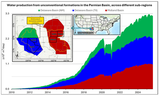
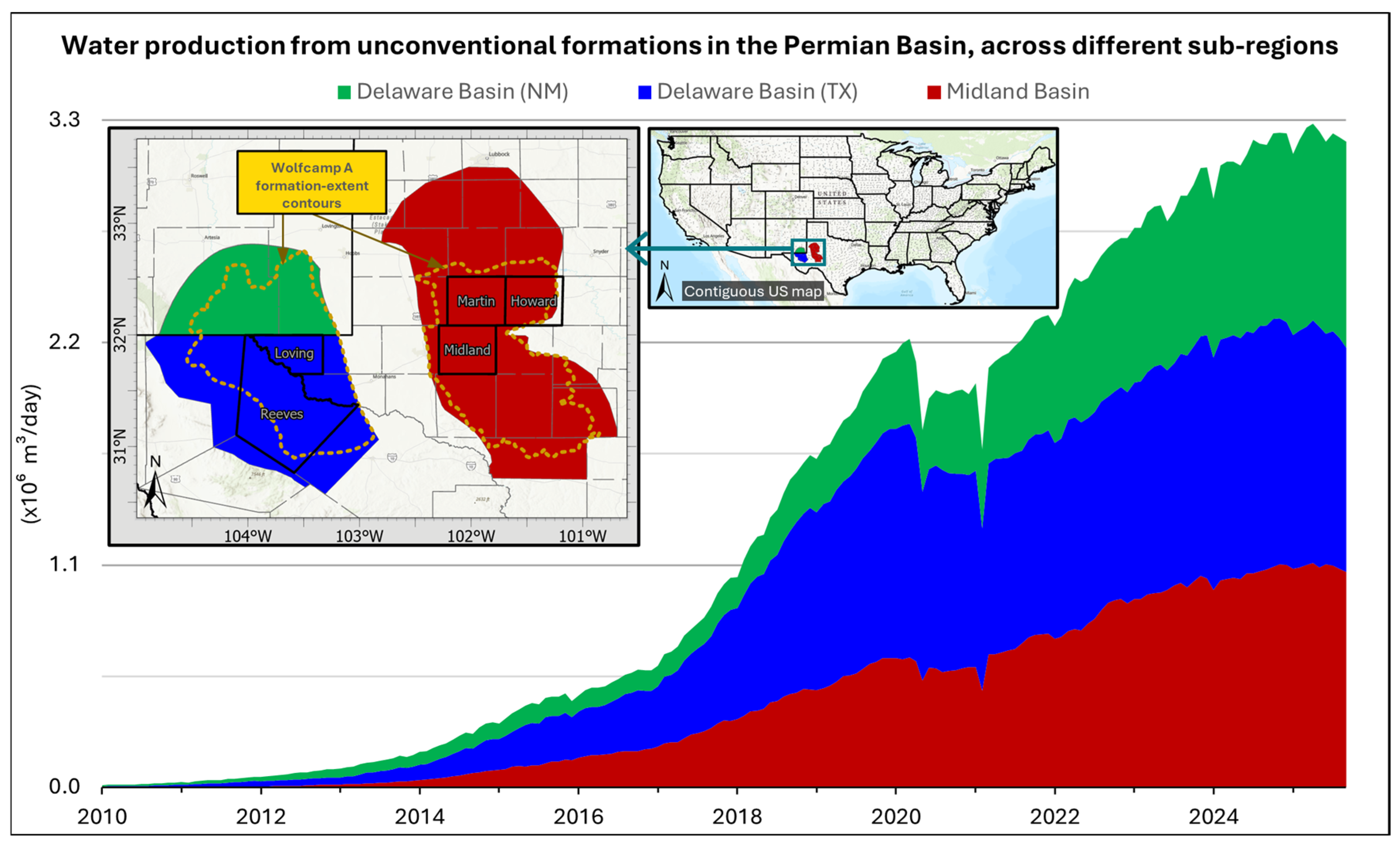
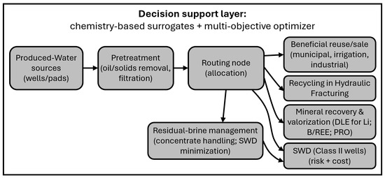
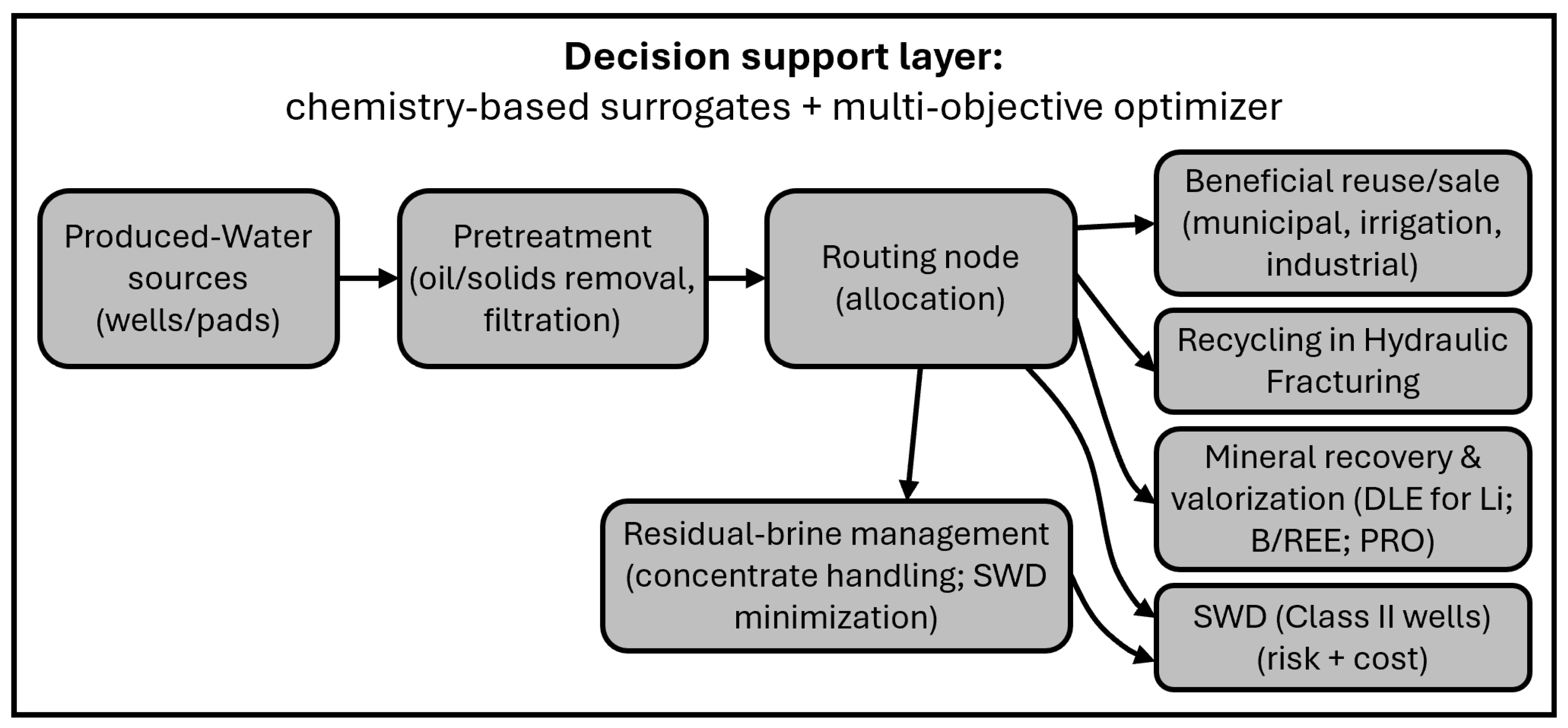
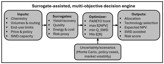
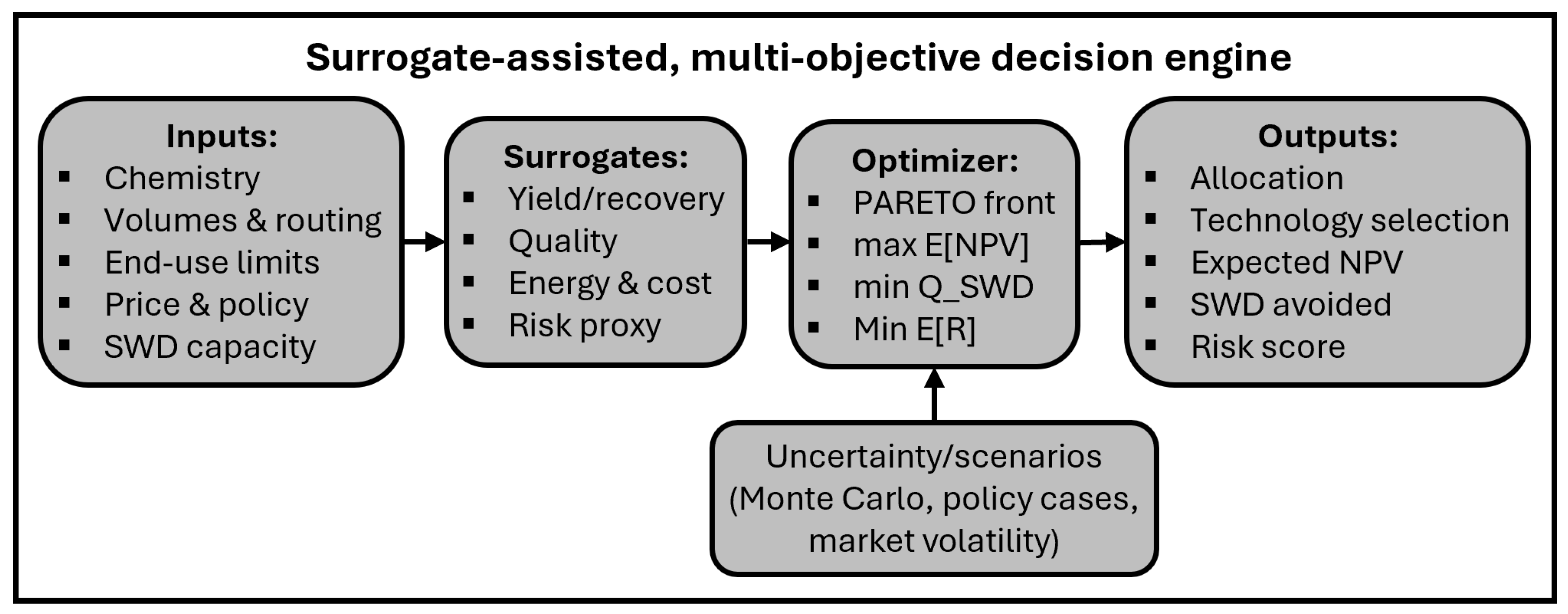
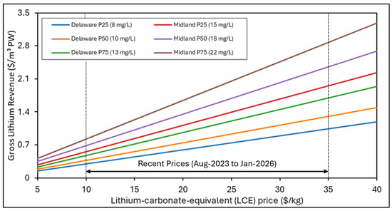
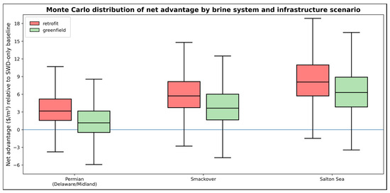
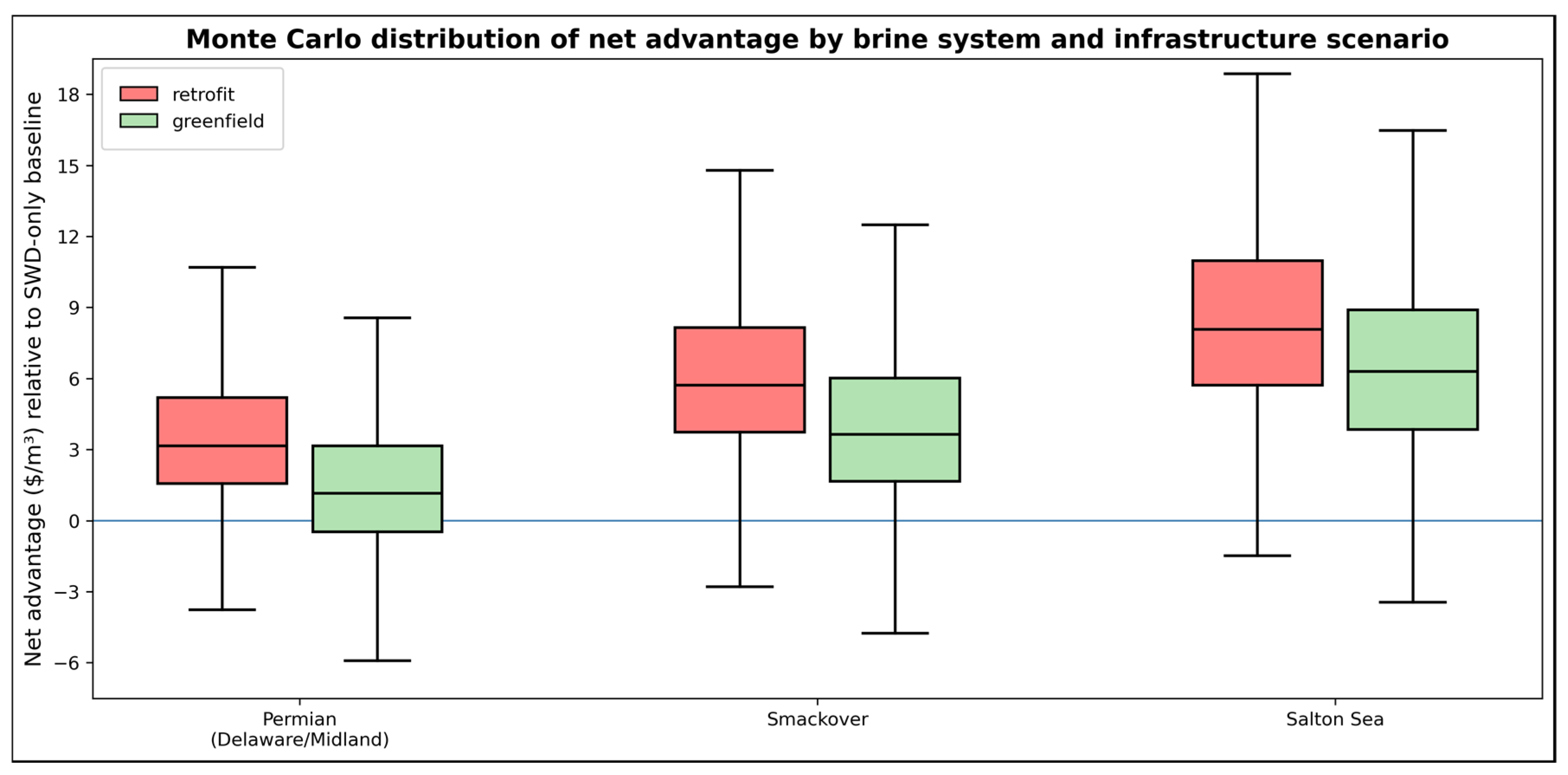

Disclaimer/Publisher’s Note: The statements, opinions and data contained in all publications are solely those of the individual author(s) and contributor(s) and not of MDPI and/or the editor(s). MDPI and/or the editor(s) disclaim responsibility for any injury to people or property resulting from any ideas, methods, instructions or products referred to in the content. |
© 2026 by the authors. Licensee MDPI, Basel, Switzerland. This article is an open access article distributed under the terms and conditions of the Creative Commons Attribution (CC BY) license.