


Abstract
Accurate runoff forecasting is vital yet challenged by the increasing non-stationarity of hydrological systems, which often exceeds the capacity of traditional single models. Ensemble forecasting, as an effective approach, integrates multiple models’ information to enhance forecasting performance and assess uncertainty. However, existing methods (such as Bayesian Model Averaging and BMA) still have limitations in dealing with complex hydrological scenarios, particularly in the construction and optimization of forecast intervals. This paper proposes a novel hydrological ensemble interval forecasting method based on constrained multi-model weight optimization (Constrained Multi-Model Weight Optimization, CMWO). CMWO utilizes a set of heterogeneous deterministic models to generate members, assigns dynamic optimization weight intervals to enhance flexibility, and employs a multi-objective framework to minimize interval width and errors subject to a ≥95% coverage constraint. Taking the Huangjinxia Reservoir in the upper reaches of the Hanjiang River as a case study, the CMWO method was systematically applied and evaluated for decadal-scale runoff forecasting and comprehensively compared with widely used BMA methods and individual models. The results show that CMWO significantly outperforms in improving point forecast accuracy (measured by RMSE, KGE, etc.) and interval forecast quality (evaluated by PICP, PIAW, CRPS, etc.), especially in generating narrower, more informative prediction intervals while ensuring high reliability. The CMWO method proposed in this study provides a competitive new tool for the effective management of forecasting uncertainty in complex hydrological systems.
1. Introduction
Accurate hydrological forecasting is fundamental for water management [1,2]. However, climate change and anthropogenic activities introduce complex non-linearities and uncertainties, making the development of advanced quantification techniques a scientific imperative [3,4].
Traditional deterministic hydrological forecasting, whether rooted in physically based conceptual or distributed models [5] or driven by data-informed statistical and machine learning approaches [6,7], has historically provided valuable predictive information. Single models are inherently constrained by structural simplifications and parameter sensitivities [8,9]. To transcend these limits, ensemble forecasting has emerged as a dominant paradigm, synergistically integrating disparate models to provide robust probabilistic distributions for risk-informed decision-making [10,11]. It provides a more comprehensive information foundation for risk-informed decision-making [12].
Bayesian Model Averaging (BMA) is a widely applied post-processing technique that assigns posterior weights to ensemble members based on historical performance [13,14]. However, the efficacy of BMA is not without its caveats. The standard BMA framework conventionally assumes that the forecast errors of ensemble members conform to a normal distribution [15,16]. This assumption often stands in contradiction to the skewed, heavy-tailed, or otherwise complex distributional characteristics frequently observed in actual hydrological series, particularly for extreme runoff events. Such discrepancies can culminate in systematic biases in the estimation of forecast intervals and a distorted representation of uncertainty attributes [17,18]. Furthermore, the estimation of BMA weights is sensitive to the quality and length of the training dataset, and in dynamically evolving hydrological systems, static weights may fail to adequately adapt to time-varying optimal model combinations. The selection of appropriate conditional probability density functions for BMA and the effective management of inter-model correlations also remain persistent challenges for researchers [19,20].
In recent years, the rapid ascendancy of machine learning, particularly deep learning methodologies, has catalyzed new breakthroughs in hydrological forecasting, capitalizing on their potent capabilities in non-linear mapping and autonomous learning of intricate patterns from voluminous datasets [21,22]. From the sophisticated capture of temporal dependencies by Recurrent Neural Networks (RNNs) and their advanced variants (e.g., LSTM, GRU) to the efficacious extraction of spatial-temporal features by Convolutional Neural Networks (CNNs), these data-driven techniques have demonstrated compelling promise in applications ranging from rainfall–runoff simulation and flood inundation forecasting to the nuanced quantification of uncertainty [23,24,25]. Nevertheless, purely data-driven models are not without their own set of challenges, including a lack of interpretability stemming from their “black-box” nature, a high dependency on data quality and representativeness, and potentially limited extrapolation capabilities beyond the domain of the training data [26]. Consequently, a prominent research frontier involves the deep integration of data-driven strengths with the a priori knowledge embedded in hydrological physics or the structured frameworks of ensemble learning, aiming for synergistic advantages [27,28,29].
Notwithstanding the substantial advancements achieved by existing ensemble methods (including BMA and its numerous refinements) and emergent machine learning techniques in the hydrological forecasting arena, several critical scientific and technical challenges persist, particularly at the operational level of interval forecasting. Specifically, a paramount objective is the conception of a new paradigm that not only fully leverages the synergistic benefits of multi-model ensembles but also transcends the limitations of conventional approaches in areas such as parameter optimization, adaptability to complex distributional characteristics, and, most critically, the construction of forecast intervals—especially in achieving the core desideratum of high-coverage probability whilst concurrently pursuing narrow interval width. Traditional methods often address point forecast accuracy and interval forecast quality as separate, uncoupled objectives, or they struggle to effectively balance the inherently conflicting goals of coverage and sharpness in interval construction. Addressing these exigent challenges, this paper endeavors to propose and systematically evaluate a novel hydrological ensemble interval forecasting method, termed Constrained Multi-model Weight Optimization (CMWO). The core design philosophy of CMWO is rooted in a profound reflection upon and an ambition to surpass the limitations of extant methodologies. Heterogeneous Base Ensemble Generation: To transcend the limitations of singular modeling paradigms, CMWO adopts a strategic integration of six diverse deterministic models, meticulously selected to provide a complementary spectrum of theoretical foundations. The synergy of this ensemble is rooted in the deep integration of physics-based insights and data-driven strengths. Specifically, the Two-Parameter Hydrological Model (TPWB) serves as the physical ‘anchor,’ ensuring that the ensemble adheres to the fundamental principles of water balance and mass conservation, which are critical for maintaining physical consistency in long-term simulations. In contrast, the Online Sequential Extreme Learning Machine (OS-ELM) and BP Neural Network (BPNN) are incorporated for their exceptional non-linear mapping capabilities, enabling the framework to autonomously learn and adapt to the increasingly non-stationary characteristics of runoff that physically based models might overlook. Furthermore, the inclusion of Support Vector Regression (SVR) and Random Forest (RF) enhances the ensemble’s robustness against data noise and structural uncertainties. By constructing this heterogeneous base, CMWO establishes a diverse error structure—a prerequisite for effective multi-objective weight optimization—thereby ensuring a more comprehensive capture of complex runoff processes from multiple analytical perspectives. Dynamic Weight Interval Optimization: Departing from the practice in traditional BMA and analogous methods, which assign a single, fixed weight to each ensemble member, CMWO innovatively assigns a dynamically optimizable weight interval (i.e., upper and lower bounds for the weight) to each constituent model. This design imbues the model combination process with substantially enhanced flexibility, empowering it to better adapt to the time-varying contributions of individual members under diverse hydrological regimes and across different forecast lead times.
Constrained Multi-Objective Optimization Framework: Most crucially, CMWO integrates the two pivotal desiderata of interval forecasting—high coverage probability (Reliability) and narrow interval width (Sharpness)—along with point forecast accuracy (Accuracy) into a unified multi-objective optimization framework. Specifically, the optimization problem is formulated to minimize the average forecast interval width (PIAW) and a measure of point forecast error (e.g., RMSE). This optimization is performed subject to a hard constraint stipulating that the coverage probability (PICP) of the forecast interval with respect to the actual observations must attain a pre-defined high threshold (e.g., ≥95%). By solving this constrained multi-objective optimization problem, CMWO endogenously and concurrently determines the optimal weight intervals for each member model and, consequently, the final ensemble forecast product.
This study applies the CMWO method to decadal-scale runoff forecasting for the Huangjinxia Reservoir in the upper Hanjiang Basin. Through multi-faceted comparisons with BMA and individual models, we elucidate its theoretical advantages in balancing reliability and sharpness, offering a refined tool for managing forecast uncertainty.
2. Study Area and Data
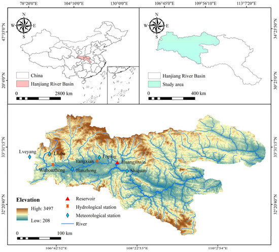
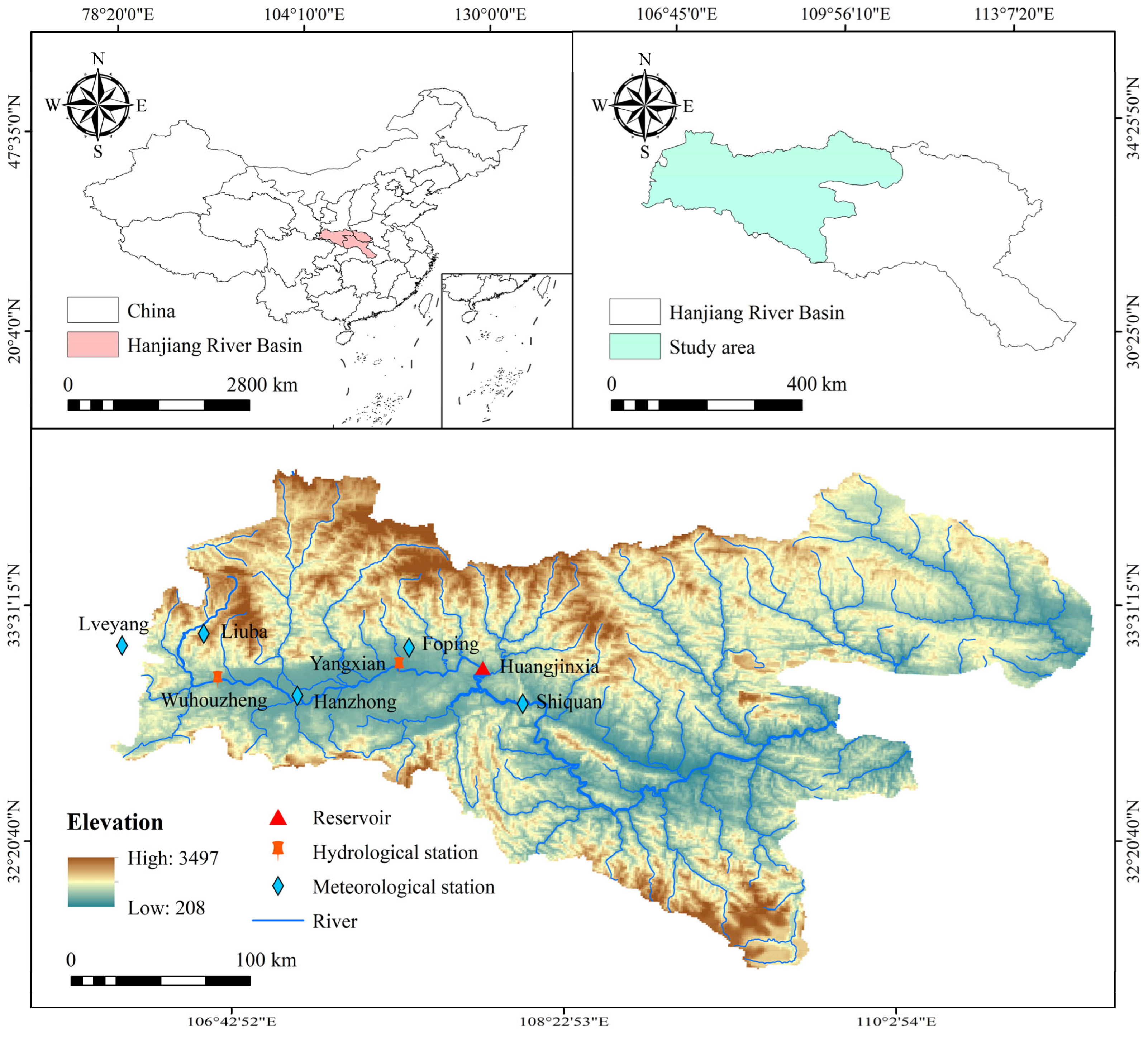
The Hanjiang River, the longest tributary of the Yangtze River, plays a crucial role in China’s sustainable water resource utilization, regional ecological balance, and socio-economic development. The focus of this research is on the upper reaches of the Hanjiang River, specifically the section within Shaanxi Province, China. The hydrological regime of this section directly influences the inflow to the Huangjinxia Reservoir, which is the primary target of this study. As shown in Figure 1, the study area is located within the Qinling–Bashan Mountains of Central-Western China, characterized by complex topography and an altitudinal range from approximately 208 m to 3497 m. This significant elevation gradient, combined with diverse geomorphological units, shapes the region’s unique hydrological cycle and climatic characteristics. The upper Hanjiang River serves not only as a critical water source conservation area and ecological barrier but also as the key water source and regulation hub for the “South-to-North Water Diversion Project’s Hanjiang to Weihe River” (Yinhanjiwei)—a major national water conservancy initiative. The Huangjinxia Reservoir is one of the core regulating reservoirs within this engineering system. Accurate forecasting of its inflow, particularly interval forecasts that quantify uncertainty, is of critical scientific and practical importance for ensuring the project’s water supply effectiveness, optimizing the joint operational strategies of reservoir cascades, and enhancing the overall water resource management and drought/flood resilience capabilities of the entire region.
Figure 1.
Study area of Hanjiang River basin of Shaanxi province.
To support the modeling and analytical efforts of this research, a comprehensive set of hydro-meteorological data covering the study area was collected. Runoff data were primarily sourced from long-term observational series at two key hydrological stations: Wuhouzhen and Yangxian (Figure 1). These stations record the discharge processes at the basin outlet or other significant control sections. Meteorological data were aggregated from historical records of several representative weather observation stations, including Lueyang, Liuba, Foping, Hanzhong, and Shiquan (Figure 1). These records primarily include meteorological elements closely related to runoff generation, such as precipitation and air temperature. The meteorological variables primarily include precipitation and air temperature, which are critical drivers for runoff generation in this basin. To ensure data integrity, a rigorous quality control procedure was implemented, including range checks and inter-station consistency checks. The runoff and meteorological sequences are 99.5% complete; for the remaining 0.5% of missing values, linear interpolation was employed to maintain continuity. Sensitivity analysis indicates that this minor data variability has a negligible impact on the deterministic model evaluation results presented in Table 1. The finalized data sequence spans from January 1975 to December 2014, comprising 1440 ten-day records. To ensure the adequacy of model training and the independence of validation, the entire dataset was rigorously partitioned following a conventional 7:3 ratio: the 1008 ten-day period data records from the first ten-day period of January 1975 to the last ten-day period of December 2002 were designated as the calibration period, used for parameter calibration, structural identification, and optimization of the various predictive models. The remaining 432 ten-day period data records, from the first ten-day period of January 2003 to the last ten-day period of December 2014, constituted the validation period, employed for the independent evaluation of the calibrated models’ forecasting performance, generalization capability, and robustness.
Table 1.
Deterministic Model Evaluation Metrics Results.
3. Methods
The core of this study lies in constructing and evaluating an ensemble runoff interval forecasting framework called Constrained Multi-model Weighting Optimization (CMWO). This framework aims to enhance the overall performance of ensemble forecasts, particularly in terms of reliability and sharpness of the forecast intervals, by optimizing the contribution weights of individual member models that constitute the ensemble. The performance of CMWO will be systematically compared with the widely used Bayesian Model Averaging (BMA) method in the field of hydrological forecasting. The prediction results of all single models serve as the input foundation for subsequent integration work.
3.1. Individual Runoff Forecasting Models
Previous case studies have demonstrated that while MLR and RF offer computational simplicity, they often struggle with highly non-stationary peak events. In contrast, models like BPNN and SVR have shown superior capability in fitting complex non-linear hydrological patterns, though they are prone to overfitting without proper regularization. By integrating these diverse theoretical foundations—ranging from conceptual water balance (TPWB) to efficient online learning (OS-ELM)—the ensemble framework aims to leverage the respective strengths of each approach while mitigating their structural limitations. To ensure that the integrated forecasting system has good diversity and can capture the complexity of the runoff process from different perspectives, this study selected six candidate models: Multiple Linear Regression (MLR), Support Vector Regression (SVR), Random Forest (RF), BP Neural Network (BPNN), Online Sequential Extreme Learning Machine (OS-ELM), and the Two-parameter Hydrological Model (TPWB).
3.2. Constrained Multi-Model Weight Optimization (CMWO) Framework
The Constrained Multi-Model Weight Optimization (CMWO) method aims to enhance the overall performance of ensemble forecasts by parameterizing and optimizing the contribution weights of each member model in the ensemble. The core components of this framework include mathematical representation of weight intervals, Monte Carlo ensemble simulation based on weight intervals, construction of a multi-objective optimization model considering prediction interval coverage constraints, and final scheme selection based on multi-attribute decision theory.
3.2.1. Weight Interval Parameterization and Monte Carlo Ensemble Simulation
The core of the CMWO method is to define the weight wj of each model j in the M member models as an interval [wj,l, wj,u] to be optimized. Among them, the lower limit of the interval wj,l and the range (width) of the interval wj,r are used as 2M decision variables directly optimized by the optimization algorithm, forming the decision vector X. The upper limit of the weight interval is derived from wj,u = wj,l + wj,r The form of the decision vector X is as follows:
Constraints are typically imposed on decision variables.
For a given decision vector X, a set forecast is generated using a Monte Carlo method that includes K independent simulations. In the k-th simulation, the weights wj(k) of each member model j are randomly sampled from their corresponding optimization interval [wj,l, wj,u] according to a uniform distribution U(wj,l, wj,u):
Subsequently, using this set of sampling weights the original forecasts ft,j (at time step of t) of each member model are linearly weighted to obtain the k-th ensemble forecast member :
where N is the length of the time series. Based on the empirical distribution constructed from K ensemble members , and according to the preset target prediction interval coverage PICPtarget (corresponding to the nominal significance level αnom = 1 − PICPtarget), the prediction interval [Lt, Ut] is constructed by taking the αnom/2 and 1 − αnom/2 quantiles of the empirical distribution:
where Pperc(S,p) represents the function to find the p-th percentile of set S. The ensemble forecast value typically takes the arithmetic mean of K ensemble members:
3.2.2. Multi-Objective Optimization Model
The core of the CMWO framework is to construct the parameter optimization problem of the weight interval as a multi-objective optimization model. This study aims to simultaneously optimize two interrelated objectives: enhancing the clarity of the prediction interval (i.e., reducing its width) and ensuring the accuracy of the ensemble point forecasts.
Objective function O1: Minimize the average width of the prediction interval (PIAW).
Objective function O2: Minimize the root mean square error (RMSE). This objective aims to improve the agreement of the ensemble point forecast values with the actual observed runoff Yt.
Constraints: To ensure that the prediction interval generated has practical significance, the actual coverage rate PICPactual(X) over the entire forecast period must not be lower than the preset target coverage rate PICPtarget:
where I(⋅) is the indicator function. It takes a value of 1 when the condition is satisfied; otherwise, it takes 0. The constraint is represented as
A penalty term ϕpenalty(X) is defined, which imposes a penalty when the actual coverage rate is below the target:
where βpenalty is a preset sufficiently large positive penalty coefficient. The objective functions with the penalty imposed are as follows:
This study employs the Non-dominated Sorting Genetic Algorithm II (NSGA-II) to solve the above bi-objective optimization problem with constraints.
3.2.3. Selection of Pareto Optimal Solutions: Multi-Criteria Decision Making (MCDM)
The output of the NSGA-II optimization process is typically a set of Pareto optimal solutions (Pareto front), where any improvement in one solution necessarily leads to the deterioration of at least one other objective. To select a final, representative implementation solution from this set of non-dominated solutions, this study introduces the Multi-Criteria Decision Making (MCDM) method. Specifically, four widely applied MCDM techniques were employed: TOPSIS (Technique for Order Preference by Similarity to Ideal Solution), VIKOR (VlseKriterijumska Optimizacija I Kompromisno Resenje), PROMETHEE II (Preference Ranking Organization Method for Enrichment Evaluations II), and COPRAS (Complex Proportional Assessment).
In this study, the relative importance (i.e., objective weights) of the two optimization objectives, PIAW and RMSE, was determined using the objective entropy weighting method, and these weights were then input into the MCDM model to select the final compromise solution. From an operational perspective, the CMWO framework is computationally efficient and executes reliably on standard desktop hardware. Given the 10-day (decadal-scale) forecasting interval used in this study, the total execution time is fully compatible with the timeframes required for routine reservoir scheduling and water resource management, ensuring its practical feasibility in real-world applications.
3.3. Bayesian Model Averaging (BMA)
The probability density function (PDF) of the BMA forecast is a weighted combination of the conditional PDFs of the ensemble members, specifically expressed as
where y is the forecast target variable (such as runoff or precipitation) and D represents the observed dataset used for model training. K is the number of models in the ensemble forecasting system. fk is the deterministic forecast provided by the k-th model. is the probability density function with fk as the conditional mean and as the conditional variance. In this study, a heteroscedastic normal distribution is adopted for , where the conditional variance is not constant but varies linearly with the forecast magnitude. This allows the model to better reflect the heteroscedastic uncertainty inherent in different runoff regimes. The weight wk quantifies the contribution of the k-th model to the final BMA forecast, with values that are non-negative and satisfy the constraint . These weights essentially reflect the posterior probability that each model becomes the “optimal” forecasting model given the training data.
BMA Parameter Estimation
The effectiveness of the BMA method largely depends on the accurate estimation of model weights wk and the conditional forecast variances of each model. These key parameters are typically derived based on the maximum likelihood estimation (MLE) principle, by maximizing the BMA log-likelihood function under the observed data during the training period. The log-likelihood function L is defined as
where θ represents the parameter vector containing all the parameters to be estimated (i.e., all wk and ), T is the length of the observational sequence during the training period; yt and fk,t represent the observed value and the forecast value of model k at time t, respectively.
Parameters were estimated via Maximum Likelihood Estimation using the DREAM algorithm (Differential Evolution Adaptive Metropolis) combined with MCMC.
3.4. Forecast Evaluation Metrics
To comprehensively evaluate the performance of forecasts generated by the CMWO method, a series of standardized evaluation metrics are employed for both deterministic and probabilistic interval forecasts. The deterministic forecast evaluation metrics primarily include Root Mean Square Error (RMSE), Mean Absolute Error (MAE), Kling–Gupta Efficiency (KGE), Coefficient of Determination (R2), and Percent Bias (PBIAS). The probabilistic interval forecast evaluation metrics include the Prediction Interval Coverage Probability (PICP, see Equation (9)) as an optimization constraint and the Prediction Interval Average Width (PIAW, see Equation (7)) as an optimization objective. Additionally, Interval Score (IS) and Continuous Ranked Probability Score (CRPS) are used for comprehensive evaluation. Through a comprehensive analysis of the above metrics, the forecast performance of the CMWO method and the BMA method can be thoroughly assessed.
4. Results
4.1. Deterministic Model Performance Evaluation
Before constructing the ensemble prediction system, the inherent performance of six deterministic models (MLR, SVR, RF, BPNN, OS-ELM, and TPWB) was independently evaluated. Each model was independently evaluated using cross-validation on the 1975–2014 dataset. Key performance indicators—RMSE, KGE, , and MAE—are summarized in Table 1.
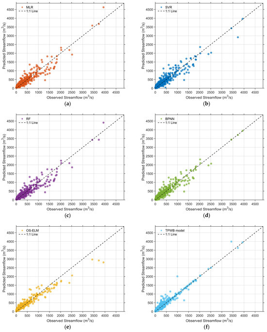
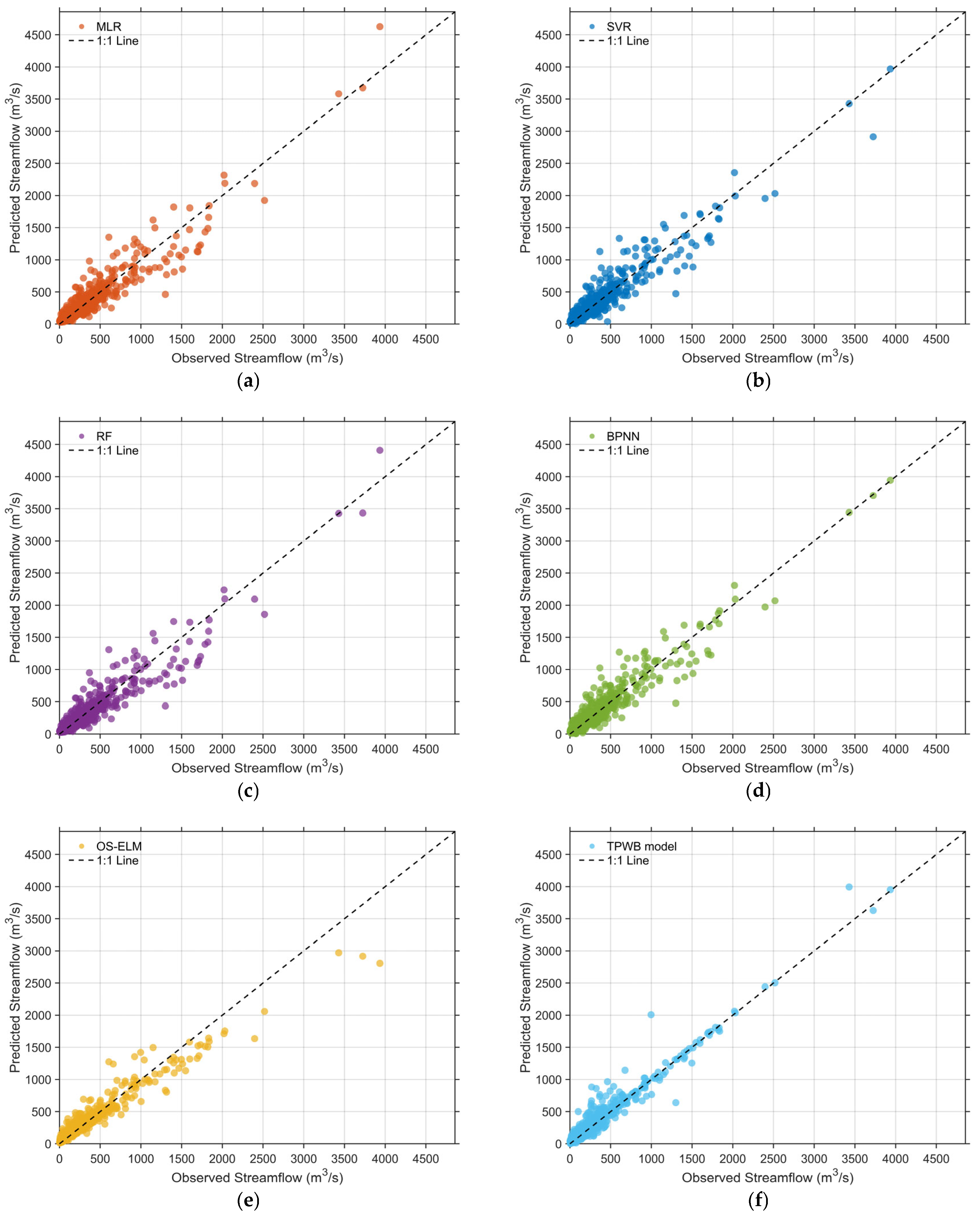
The results reveal distinct predictive capabilities among the models. The TPWB model exhibits the best overall performance, demonstrating a superior ability to capture the primary hydrological patterns of the watershed. The OS-ELM model ranks second in terms of RMSE and , though its lower KGE suggests minor deviations in simulating specific statistical properties of the flow process. Both BPNN and SVR show robust performance, consistently outperforming the linear MLR and decision-tree-based RF models. Scatter plots in Figure 2 supplement these findings, showing that TPWB results cluster most closely around the 1:1 line. These performance disparities and the resulting prediction diversity establish a robust foundation for building an effective ensemble system. It is particularly noteworthy that the TPWB model, despite its minimalist structure with only two parameters, achieved the highest deterministic accuracy among all candidate models. This suggests that for the upper Hanjiang basin, structural parsimony rooted in physical laws may offer greater robustness than algorithmic complexity alone. The underlying physical mechanisms and the ‘power of parsimony’ that lead to this superior performance are further explored in the Discussion section (Section 5.1).
Figure 2.
Scatter plots of predicted versus measured values for six single deterministic models: (a) MLR; (b) SVR; (c) RF; (d) BPNN; (e) OS-ELM; (f) TPWB model.
4.2. Overall Performance Comparison of Ensemble Prediction Models
Table 2 summarizes the BMA method and the evaluation indicators of the CMWO model optimized by four MCDM methods during the training and validation periods.
Table 2.
Performance evaluation indicators of the BMA ensemble forecast model and the CMWO ensemble forecast model selected by MCDM during the training and validation periods.
4.2.1. Comparison and Analysis of Evaluation Metrics
Figure A1 represents the evaluation results of simulated and measured values of different models at the training stage. See Appendix A for details. We found that during the training phase, the BMA method demonstrates superior point prediction accuracy and overall probabilistic forecasting quality due to its direct likelihood maximization mechanism. While CMWO variants achieve higher PICP values, their point accuracy is slightly lower and intervals are relatively wider, indicating that BMA fits training data with higher precision. During the critical validation period, performance differences reveal the generalization capabilities of each strategy. While BMA maintains a leading position in most point prediction metrics, its PICP significantly drops. Given the typically skewed and heavy-tailed nature of runoff series, this deterioration is expected; the heteroscedastic normal distribution assumed in the BMA framework struggles to fully encompass the extreme tails of the actual distribution. This highlights a limitation of parametric approaches in capturing total uncertainty compared to the distribution-free CMWO method. In contrast, the CMWO framework maintains a high coverage rate through explicit PICP constraint optimization. Notably, CMWO-PROMETHEE and CMWO-TOPSIS not only maintain high PICP but also achieve better PIAW and far superior ISs compared to BMA (Table 2), demonstrating the potential of the CMWO framework to generate reliable and clearer prediction intervals. CMWO-PROMETHEE also shows competitive, comprehensive point prediction capabilities. Thus, while BMA excels in average point accuracy, CMWO offers unique value in providing forecasts with guaranteed coverage and superior interval quality.
4.2.2. Visualization Analysis of Prediction Process and Scatter Plots
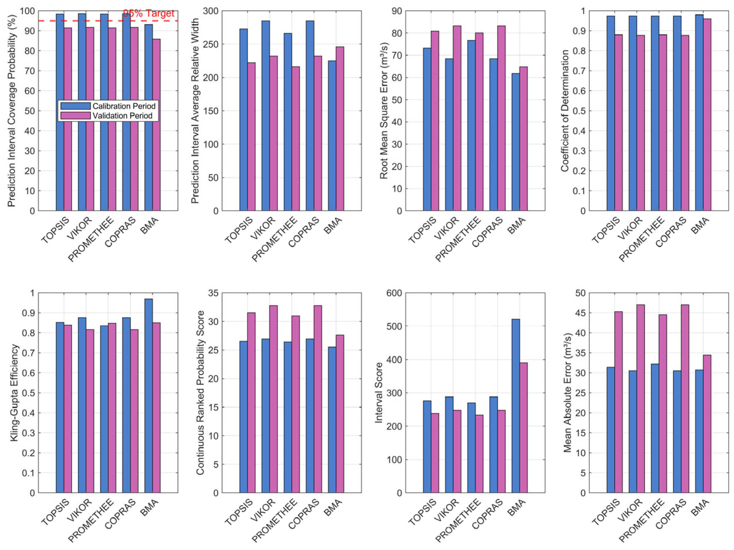
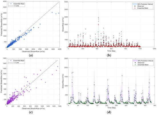
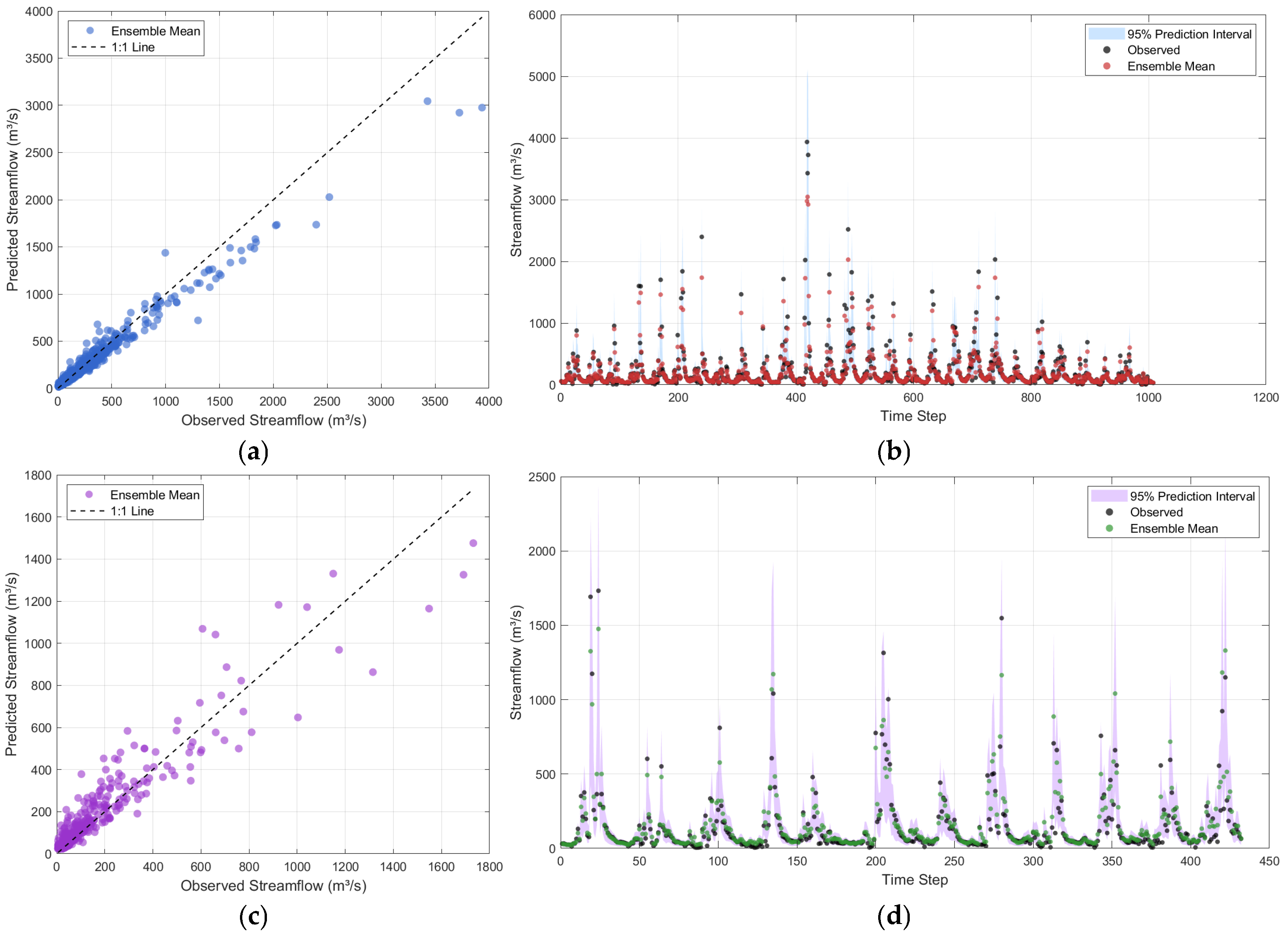
The visualization results in Figure 3 provide intuitive evidence for the quantitative indicators. CMWO-PROMETHEE prediction intervals effectively envelop observed runoff across both phases, maintaining a dynamic capture of the primary runoff processes. Scatter plots further confirm strong linear correlations between predicted and observed values, although systematic biases at specific flow levels provide clues for future model improvements. To provide a more systematic and objective foundation for the performance comparison, Figure A2 in Appendix B illustrates the statistical distribution of eight key metrics across the calibration and validation phases. This visualization reveals a critical ‘performance decay’ in the BMA method: while it achieves optimal RMSE and PICP during calibration, its reliability significantly deteriorates upon entering the validation period, with PICP falling below the 95% target. In contrast, the CMWO variants exhibit a highly stable ‘performance envelope’, maintaining consistent coverage and significantly lower Interval Scores (IS) across both stages. By mapping these statistical shifts onto a comprehensive bar chart, the generalization advantage of the CMWO framework is quantified objectively, moving beyond qualitative process–plot interpretations.
Figure 3.
CMWO-PROMETHEE Training and Validation Period: Measured and Predicted Mean Scatter Plot with Prediction Interval Process Visualization. (a) CMWO-PROMETHEE Training Period Predicted Mean vs. Measured Scatter Plot. (b) CMWO-PROMETHEE training period prediction interval. (c) CMWO-PROMETHEE Validation Period Predicted Mean vs. Measured Scatter Plot. (d) CMWO-PROMETHEE Validation period prediction interval.
4.3. Specialized Evaluation of Peak Traffic Prediction Performance
To evaluate performance under extreme conditions, the maximum 10-day discharge from each hydrological year was extracted as ‘Peak Flow’ using the Annual Maximum Series (AMS) method. The evaluation of these selected peaks (Table 3) illustrates the core trade-offs of different integration strategies in extreme event forecasting.
Table 3.
CMWO Integrated Model vs. BMA Model in Special Assessment of Peak Events.
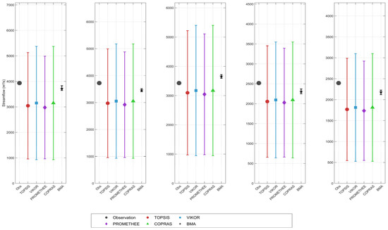
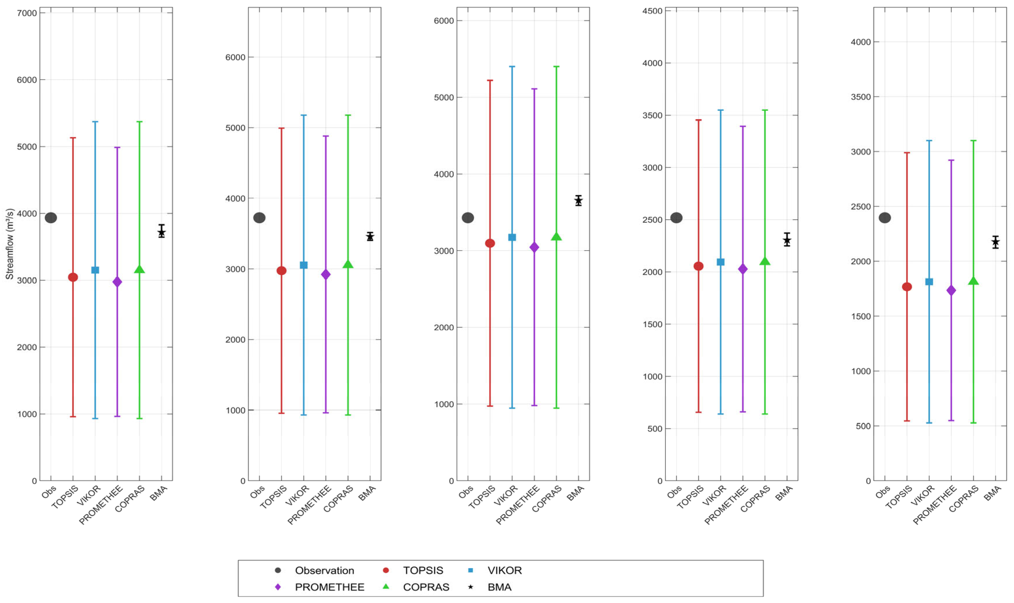
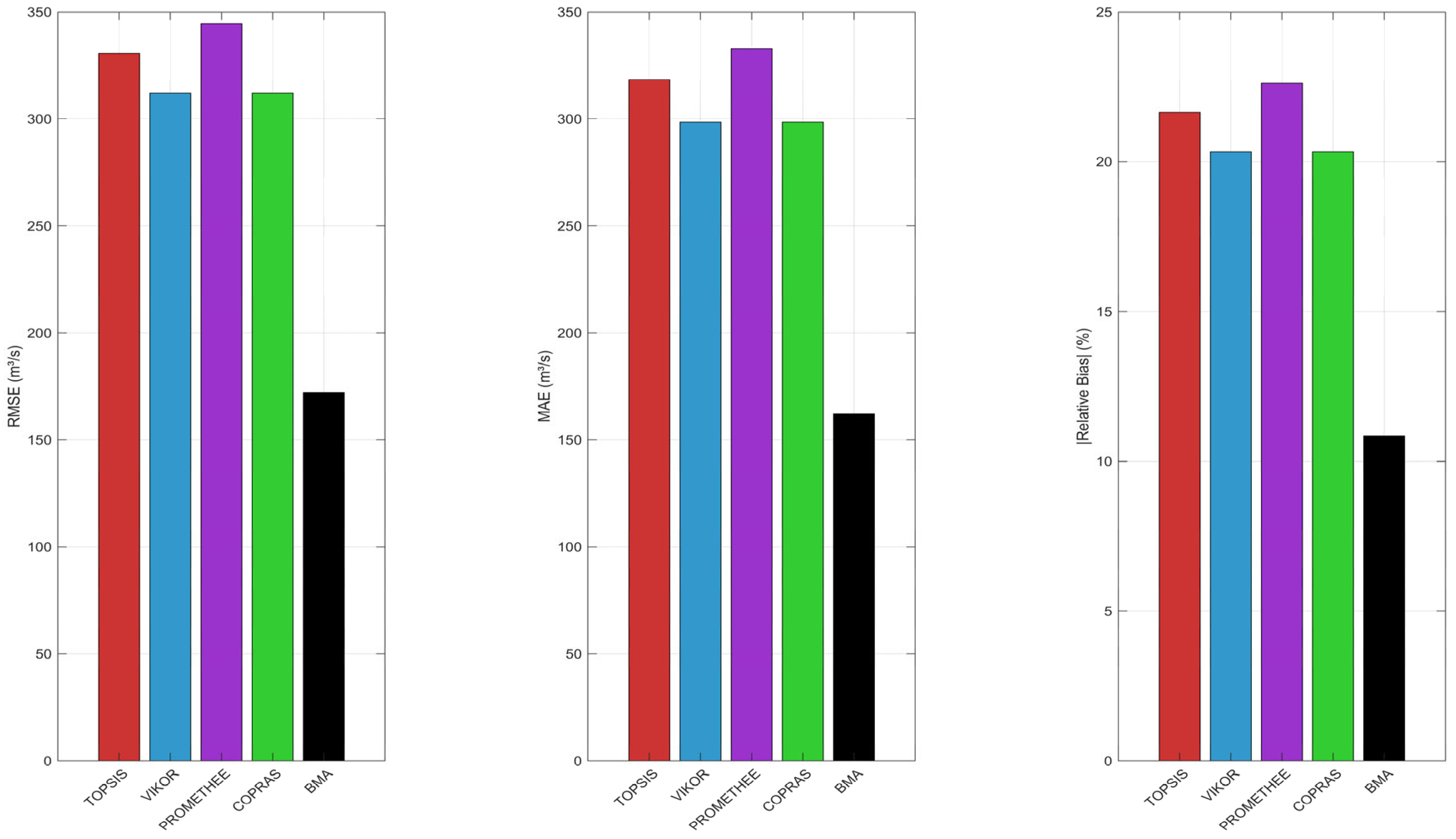
As shown in Figure 4, BMA significantly outperforms all CMWO variants in terms of peak point prediction accuracy (Peak RMSE and Peak MAE). For example, as shown in Table 3, its Peak RMSE during the validation period (121.08 m3 s−1) is much lower than that of the CMWO models (generally above 190 m3 s−1). This indicates that BMA can more accurately estimate the average magnitude of flood peaks. However, this advantage in point prediction comes with a lower peak coverage rate (Peak PICP of only 69.77% during the validation period). As shown in Figure 4, combined with observations of high-flow hydrographs, the relatively narrow prediction intervals of BMA can accurately bracket the peak in some cases but may completely miss the envelope of extreme peak floods in others.
Figure 4.
Visualization of the prediction process of 5 integrated models under 5 selected peak flow conditions.
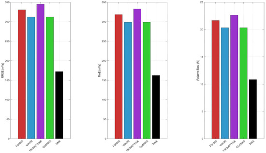
In contrast, Figure 5 represents the point prediction metrics of the mean predicted values from 5 integrated prediction models at the selected 5 peak flow levels. As shown in Figure 5, the CMWO framework, by design, prioritizes ensuring coverage of peak events. All CMWO variants achieved close to or 100% Peak PICP during both the training and validation periods. This extremely high reliability comes at the cost of significantly increasing the interval width: the Peak PIAW values of CMWO are very large (e.g., the Peak PIAW of CMWO-PROMETHEE during the validation period is as high as 868.04 m3 s−1, more than three times that of BMA). Additionally, the Peak Relative Bias (%) metric shows that most CMWO variants tend to underestimate flood peaks during the training period (e.g., CMWO-PROMETHEE at −10.20%), and this bias is adjusted but still present during the validation period. Therefore, CMWO provides a strategy to “ensure capture” of flood peaks, but its forecast intervals are very wide, potentially providing relatively vague magnitude information for practical emergency response. BMA, on the other hand, provides a more precise estimate of flood peak magnitudes, but its interval coverage reliability is lower, with a risk of underreporting.
Figure 5.
Point prediction metrics of the mean predicted values from 5 integrated prediction models at the selected 5 peak flow levels (RMSE of predicted peak vs. measured peak, MAE of predicted peak vs. measured peak, total deviation of predicted peak vs. measured peak).
4.4. Analysis of Optimal Weight Intervals for Member Models Across MCDM Schemes
Table 4 reveals the optimal weight intervals [wjd, wjd + wjr] assigned to each individual model in the selected CMWO schemes using different MCDM methods.
Table 4.
Optimal weight intervals for each sub-model of the selected CMWO schemes using different MCDMs.
Most notably, the OS-ELM model (Model 5) achieved the highest lower bound of the weight interval (wjd ≈ 0.28) and the widest range of weight adjustment (with large wjr values, making wjd + wjr far exceed other models) in all four MCDM methods’ selected schemes. This strongly suggests that OS-ELM is the most significant and critical foundational model in the CMWO framework of this study, with its prediction results having a dominant influence on the final ensemble forecast, and the optimization process assigning greater weight flexibility to adapt to different data characteristics. In contrast, the weight intervals for MLR, SVR, RF, and BPNN are relatively narrow and small, indicating that they play a supplementary or supportive role in these optimization schemes, with stable but potentially limited contributions. The TPWB model exhibits a medium and variable weight interval, especially under the TOPSIS and PROMETHEE schemes, where its weight adjustment range is wider, implying that the TPWB model may have indispensable predictive value in specific hydrological scenarios, with its importance fluctuating based on the MCDM decision preferences. This difference in weight structure also reflects the subtle variations in how different MCDM methods characterize each foundational model when balancing multiple objectives.
5. Discussion
5.1. A Comprehensive Evaluation of the Superiority and Uncertainty of Integrated Forecasting Strategies
Accurate runoff forecasting is vital for water management, yet the steep topography of the Qinling–Bashan Mountains introduces rapid flow concentration and non-stationarity that challenge traditional models. CMWO addresses these structural deficiencies by synergistically aggregating diverse model information, effectively reducing uncertainties amplified by complex mountain terrains. Compared to individual members and BMA, the NSGA-II optimized CMWO paradigm consistently demonstrates superior performance across key metrics like RMSE, KGE, and CRPS. It enhances both point accuracy and the characterization of overall probabilistic distributions. The Superiority of Physical Parsimony in Watershed Modeling: Within the single-model evaluations, a standout finding is the exceptional performance of the TPWB model, which achieved the lowest RMSE and MAE among all candidates. This superiority is primarily attributed to the strong hydraulic connectivity and relatively clear physical mechanisms inherent in the upper Hanjiang River basin. In this study area, where runoff generation follows well-defined precipitation–storage–discharge relationships, the mass balance equations within the TPWB model act as essential ‘physical guardrails’. While data-driven models like OS-ELM or BPNN possess powerful non-linear mapping capabilities, they can be sensitive to data noise and prone to overfitting when explicit physical constraints are absent. For the inflow to the Huangjinxia Reservoir, the TPWB model’s structural simplicity effectively filters out stochastic noise and captures the dominant hydrological signal, demonstrating that professional physical insights remain irreplaceable in accurately characterizing basins with robust hydraulic continuity. By optimizing PICP and PIAW under a hard coverage constraint, CMWO balances reliability and sharpness. Results show high confidence levels (PICP up to 93.75% and 90.51%) with compact intervals (PIAW of 209.83 and 245.17 m3 s−1 for training and validation), providing reliable support for reservoir scheduling and risk management. Furthermore, the weight interval optimization results (Table 4) reveal that the Online Sequential Extreme Learning Machine (OS-ELM) possesses the widest weight range. From a hydrological perspective, this reflects the model’s dynamic adaptability to the high-flow and low-flow regimes of the Hanjiang River. During the flood season, runoff processes exhibit strong non-linearity and volatility due to rapid precipitation–runoff responses in the Qinling–Bashan terrain. The wide weight interval allows CMWO to significantly increase OS-ELM’s contribution to capture these abrupt non-linear signals. Conversely, during the dry season, where runoff is dominated by stable groundwater recession, the optimization algorithm can shrink the effective weight of OS-ELM to maintain stability. The wide range of OS-ELM weights thus acts as a mathematical ‘buffer,’ enabling the integrated framework to flexibly adjust its reliance on data-driven non-linear mapping in response to the varying predictability of different hydrological seasons.
5.2. The Role and Comparative Analysis of Multi-Attribute Decision-Making Methods in Selecting from the Pareto Solution Set
Selecting optimal solutions from the Pareto front generated by multi-objective algorithms (e.g., NSGA-II) is critical for applying theoretical forecasts to real-world water management. This study employs four representative MCDM methods—TOPSIS, VIKOR, PROMETHEE II, and COPRAS—to systematically evaluate the CMWO solution set from diverse decision perspectives. Results indicate that while weight assignment influences outcomes (Table 2), the unique operational mechanisms of each method provide flexibility for various needs. Specifically, TOPSIS balances proximity to ideal solutions; VIKOR maximizes group utility; PROMETHEE II utilizes preference functions; and COPRAS evaluates proportional attribute performance. This methodological diversity allows decision-makers to balance prediction interval reliability (PICP) against sharpness (PIAW) according to their specific operational priorities. To provide actionable insights for hydrological risk management, this study offers recommendations based on specific decision objectives. For scenarios prioritizing high reliability and risk aversion (e.g., extreme event mitigation where underestimation is critical), CMWO-PROMETHEE is the preferred configuration due to its robust performance and stable coverage on the validation set. Conversely, for objectives focused on multi-attribute utility and balanced precision, VIKOR or COPRAS may serve as more suitable alternatives.
5.3. Peak Flow Forecasting: Intrinsic Challenges and Forward-Looking Improvement Strategies
Accurate peak forecasting is vital for flood management and reservoir scheduling. Despite CMWO’s overall success, capturing extreme peaks remains a challenge (Table 3), as some methods fail to reach the ideal 100% Peak PICP despite narrower intervals.
This deficiency stems from the scarcity of extreme events in historical data, leading to insufficient learning samples, and the ‘smoothing’ effect of objective functions (RMSE, PIAW) that prioritize overall accuracy over extreme peaks. An intrinsic trade-off exists within the CMWO framework: ensuring near-perfect coverage of extreme magnitudes inevitably results in a significant increase in the Prediction Interval Average Width (PIAW). This strategy prioritizes reliability over sharpness, which is essential for safety-critical applications. However, it must be acknowledged that pursuing 100% coverage may lead to excessively wide intervals and a subsequent loss of forecasting utility for high-precision requirements. Beyond magnitude discrepancies, the phase lag (timing error) of peak flows represents another critical challenge in decadal-scale forecasting. In this study, while the CMWO-based point forecasts (ensemble mean) occasionally exhibit a minor temporal displacement during rapid recession processes, the probabilistic intervals generated by CMWO demonstrate a degree of temporal robustness. Specifically, the wider forecast intervals at the peak often encapsulate the temporal shift in the actual flood pulse, thereby mitigating the operational risks associated with timing errors. However, relying solely on RMSE may mask these phase issues; thus, incorporating specific peak timing error metrics remains a vital direction for enhancing the dynamic synchronization of the forecasting framework. Future research should integrate peak-specific optimization objectives (e.g., relative error, timing), asymmetric loss functions, or specialized deep learning models that excel in extreme event simulation into the ensemble framework. The fundamental mechanistic difference lies in the optimization objective. BMA utilizes a likelihood-based mechanism that seeks to maximize the probability of the observed data, which inherently prioritizes the conditional mean and often ‘shrinks’ the interval toward high-frequency flow ranges. Conversely, CMWO employs a constraint-driven mechanism that explicitly imposes a 95% coverage threshold (PICP) during optimization. This mechanism ensures that the weight intervals are optimized to encompass extreme tail values, providing the ‘capture capability’ for peak flows that BMA lacks, even at the expense of wider intervals.
6. Conclusions
This study successfully developed and empirically validated an innovative integrated runoff interval forecasting framework (CMWO-MCDM) that combines multi-objective optimization (NSGA-II) with multi-criteria decision-making (MCDM). It was effectively applied to decadal-scale forecasting of inflow runoff at the Huangjinxia Reservoir in the upper Hanjiang River. Compared to six single benchmark models (MLR, SVR, RF, BPNN, OS-ELM, TPWB) and the commonly used BMA method, the CMWO ensemble model introduced in this study shows systematic and significant advantages in both point forecasting accuracy (measured by indicators like RMSE, KGE, and R2) and interval forecasting quality (assessed by PICP, PIAW, and CRPS). By strategically incorporating four mainstream MCDM methods (TOPSIS, VIKOR, PROMETHEE II, and COPRAS) and combining them with entropy weighting, standard deviation, and equal weighting techniques to thoroughly analyze and rank the Pareto non-inferior solution set from NSGA-II, a clear, standardized, and operational systematic approach is provided. This enables decision-makers to select the final forecasting scheme from complex multi-objective optimization results in a scientific and efficient manner. Moreover, the current study is based on six representative machine learning and hydrological models to construct the integrated system. Future research could actively consider incorporating more diverse and cutting-edge predictive models, especially various deep learning architectures (e.g., Transformer, Informer, etc.) that have shown strong potential in time series forecasting in recent years, to further broaden the upper limit of integrated forecasting performance. The focus of this study is primarily on uncertainties arising from model parameters and structural differences. Future research should aim to integrate uncertainties more systematically from input data (e.g., meteorological elements such as rainfall and evaporation, which inherently carry uncertainties) and the structural uncertainties of hydrological models into the overall interval forecasting framework, thereby achieving a more comprehensive and accurate depiction of total forecasting uncertainty.
Author Contributions
Conceptualization, X.Y. and S.Z.; methodology, Y.G., X.Y. and S.Z.; software, Y.G.; formal analysis, Y.G.; investigation, X.Y. and S.Z.; data curation, S.Z.; writing—original draft preparation, Y.G., X.Y. and S.Z.; writing—review and editing, X.Y. and S.Z.; funding acquisition, X.Y. and S.Z. All authors have read and agreed to the published version of the manuscript.
Funding
This research was jointly Supported by the Open Research Fund Program of State Key Laboratory of Water Disaster Prevention (2025490211), the National Key R&D Program of China (2023YFC3006504), the National Natural Science Foundation of China (42201047), Research and Application of Key Technologies for Multi-source Stereoscopic Monitoring-Intelligent Forecasting and Early Warning-Matrix-based Management for Reservoir Safety (37000000025001720250245), the China Postdoctoral Science Foundation (2022M711025), the Jiangsu Funding Program for Excellent Postdoctoral Talent (2022ZB175), and the Fundamental Research Funds for the Central Universities (B230201036).
Data Availability Statement
The original contributions presented in this study are included in the article. Further inquiries can be directed to the corresponding author.
Conflicts of Interest
The authors declare no conflicts of interest.
Appendix A
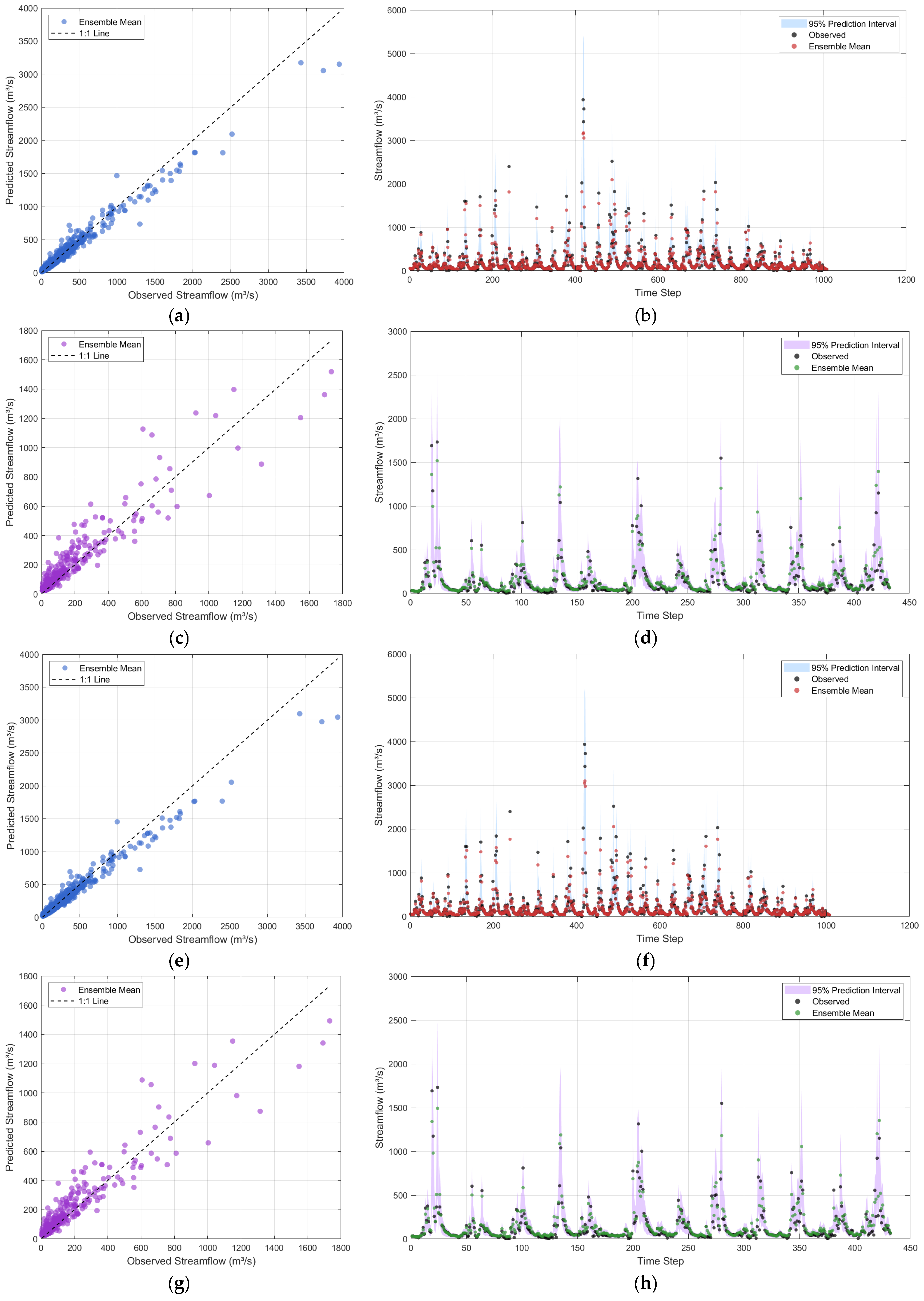
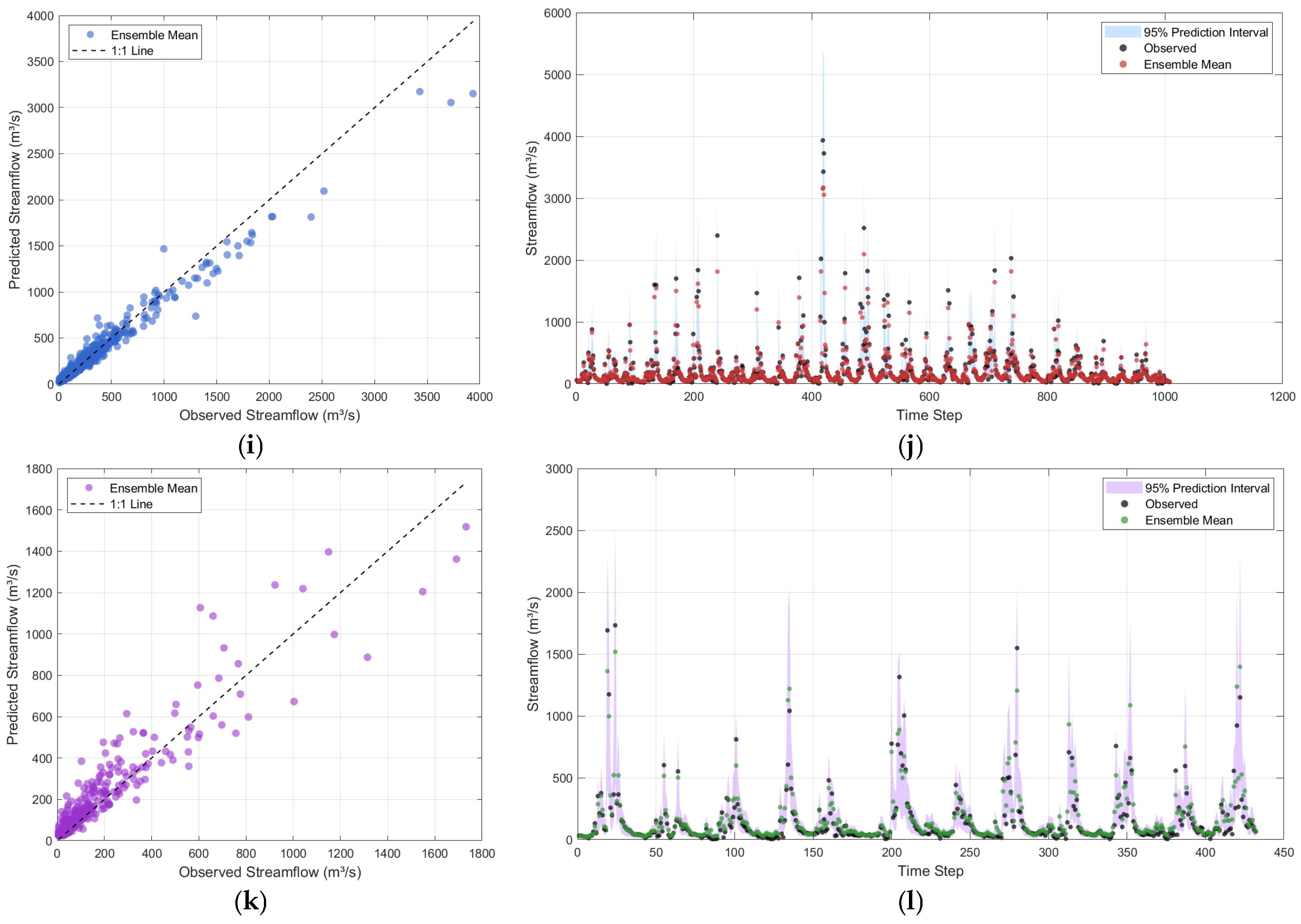
Figure A1.
(a) CMWO-COPRAS Training Period Predicted Mean vs. Measured Scatter Plot. (b) CMWO-COPRAS training period prediction interval. (c) CMWO-COPRAS Validation Period Predicted Mean vs. Measured Scatter Plot. (d) CMWO-COPRAS Validation period prediction interval. (e) CMWO-TOPSIS Training Period Predicted Mean vs. Measured Scatter Plot. (f) CMWO-TOPSIS training period prediction interval. (g) CMWO-TOPSIS Validation Period Predicted Mean vs. Measured Scatter Plot. (h) CMWO-TOPSIS Validation period prediction interval. (i) CMWO-VIKOR Training Period Predicted Mean vs. Measured Scatter Plot. (j) CMWO-VIKOR training period prediction interval. (k) CMWO-VIKOR Validation Period Predicted Mean vs. Measured Scatter Plot. (l) CMWO-VIKOR Validation period prediction interval.
Appendix B
Figure A2.
Comprehensive statistical comparison of deterministic and probabilistic evaluation metrics for BMA and CMWO variants during calibration and validation periods.
References
- Earll, M.M.; Henson, W.R.; Lockwood, B.; Boyce, S.E. Evaluating Seawater Intrusion Forecast Uncertainty under Climate Change in the Pajaro Valley, California. J. Hydrol. 2024, 636, 131226. [Google Scholar] [CrossRef] [Scilit]
- Focaccia, S.; Panini, G.; Pedrazzoli, P.; Ciriello, V. A Meta-Modeling Approach for Hydrological Forecasting under Uncertainty: Application to Groundwater Nitrate Response to Climate Change. J. Hydrol. 2021, 603, 127173. [Google Scholar] [CrossRef] [Scilit]
- Zhou, S.; Wang, Y.; Su, H.; Chang, J.; Huang, Q.; Li, Z. Dynamic Quantitative Assessment of Multiple Uncertainty Sources in Future Hydropower Generation Prediction of Cascade Reservoirs with Hydrological Variations. Energy 2024, 299, 131447. [Google Scholar] [CrossRef] [Scilit]
- Taia, S.; Scozzari, A.; Erraioui, L.; Kili, M.; Mridekh, A.; Haida, S.; Chao, J.; El Mansouri, B. Comparing the Ability of Different Remotely Sensed Evapotranspiration Products in Enhancing Hydrological Model Performance and Reducing Prediction Uncertainty. Ecol. Inform. 2023, 78, 102352. [Google Scholar] [CrossRef] [Scilit]
- Imhoff, R.O.; Buitink, J.; Van Verseveld, W.J.; Weerts, A.H. A Fast High Resolution Distributed Hydrological Model for Forecasting, Climate Scenarios and Digital Twin Applications Using Wflow_sbm. Environ. Model. Softw. 2024, 179, 106099. [Google Scholar] [CrossRef] [Scilit]
- Menapace, A.; Rodrigues, A.F.; Dalla Torre, D.; Larcher, M.; Herrera, M.; Brentan, B. Sensors Prioritisation for Hydrological Forecasting Based on Interpretable Machine Learning. J. Hydrol. 2025, 663, 134015. [Google Scholar] [CrossRef] [Scilit]
- Zhan, S.; Ye, A.; Wu, L.; Zhao, C. Ensemble Post-Processing of Sub-Seasonal to Seasonal Precipitation Forecasts Based on a Novel Probabilistic Double Machine Learning Method. J. Hydrol. 2025, 660, 133484. [Google Scholar] [CrossRef] [Scilit]
- Davidson-Chaput, J.; Arsenault, R.; Martel, J.-L.; Troin, M. Value of Various Elements of the Hydrological Forecasting Chain: Is There a Successful Pathway for Improving the Overall Performance? J. Hydrol. 2025, 658, 133186. [Google Scholar] [CrossRef] [Scilit]
- Panchanathan, A.; Ahrari, A.; Ghag, K.S.; Mustafa, S.; Haghighi, A.T.; Kløve, B.; Oussalah, M. An Overview of Approaches for Reducing Uncertainties in Hydrological Forecasting: Progress and Challenges. Earth-Sci. Rev. 2024, 258, 104956. [Google Scholar] [CrossRef] [Scilit]
- Fallah Kalaki, M.; Delavar, M.; Farokhnia, A.; Morid, S.; Shokri Kuchak, V.; Hajihosseini, H.; Shahbazi, A.; Nourmohammadi, F.; Motamedi, A.; Eini, M.R. An Ensemble Multi-Model Approach for Long-Term River Flow Forecasting in Managed Basins of the Middle East: Insights from the Karkheh River Basin. J. Hydrol. 2025, 654, 132846. [Google Scholar] [CrossRef] [Scilit]
- Nikhil Teja, K.; Manikanta, V.; Das, J.; Umamahesh, N.V. Enhancing the Predictability of Flood Forecasts by Combining Numerical Weather Prediction Ensembles with Multiple Hydrological Models. J. Hydrol. 2023, 625, 130176. [Google Scholar] [CrossRef] [Scilit]
- Tadayon, A.; Nazari, M.; Kerachian, R. Enhancing Long-Lead Rainfall Forecasting in Data-Scarce Large Watersheds Using Multi-Model Fusion. J. Hydrol. Reg. Stud. 2025, 62, 102936. [Google Scholar] [CrossRef] [Scilit]
- Wang, X.; Deng, C.; Yin, X.; Wei, J.; Zou, J. Assessing Climate Change Impacts on Streamflow in Upper Han River Basin Using Deep Learning Models Ensembled with Bayesian Model Averaging. Water Sci. Eng. 2025, 18, 412–421. [Google Scholar] [CrossRef] [Scilit]
- Huang, Y.-J.; Lee, Y.-Y.; Chang, H.-L.; Wang, C.; Hong, J.-S.; Hsiao, C.K. Bayesian Typhoon Precipitation Prediction with a Mixture of Ensemble Forecast-Based and Historical Event-Based Prediction Functions. J. Hydrol. 2024, 635, 131176. [Google Scholar] [CrossRef] [Scilit]
- Zhang, J.; Li, W.; Duan, Q. Quantifying the Contributions of Hydrological Pre-Processor, Post-Processor, and Data Assimilator to Ensemble Streamflow Prediction Skill. J. Hydrol. 2025, 651, 132611. [Google Scholar] [CrossRef] [Scilit]
- Quilty, J.; Jahangir, M.S.; You, J.; Hughes, H.; Hah, D.; Tzoganakis, I. Bayesian Extreme Learning Machines for Hydrological Prediction Uncertainty. J. Hydrol. 2023, 626, 130138. [Google Scholar] [CrossRef] [Scilit]
- Lombardo, L.; Papalexiou, S.M.; Thébault, C.; Clark, M.P.; Vogel, R.M.; Viglione, A. Residual Dynamics in Hydrological Models: Insights from a Large Sample of Catchments and Models. Adv. Water Resour. 2025, 206, 105165. [Google Scholar] [CrossRef] [Scilit]
- Bazrafshan, O.; Ehteram, M.; Moshizi, Z.G.; Jamshidi, S. Evaluation and Uncertainty Assessment of Wheat Yield Prediction by Multilayer Perceptron Model with Bayesian and Copula Bayesian Approaches. Agric. Water Manag. 2022, 273, 107881. [Google Scholar] [CrossRef] [Scilit]
- Zhu, S.; Zha, G.; Wang, Q.; Ma, S.; Qin, H. A High Performance Assimilation of Surface Soil Moisture Based on a Hybrid Framework of Machine Learning and Physical Hydrological Model. J. Hydrol. 2026, 664, 134513. [Google Scholar] [CrossRef] [Scilit]
- Ciupak, M.; Ozga-Zielinski, B.; Adamowski, J.; Quilty, J.; Khalil, B. The Application of Dynamic Linear Bayesian Models in Hydrological Forecasting: Varying Coefficient Regression and Discount Weighted Regression. J. Hydrol. 2015, 530, 762–784. [Google Scholar] [CrossRef] [Scilit]
- Zhu, F.; Zhu, O.; Han, M.; Liu, W.; Guo, X.; Hou, T.; Zhao, L.; Xu, C.; Zhong, P. A Hybrid Process-Data Driven Framework for Real-Time Hydrological Forecasting with Interpretable Deep Learning. J. Hydrol. 2025, 662, 134082. [Google Scholar] [CrossRef] [Scilit]
- Khatun, A.; Jena, P.P.; Sahoo, B.; Chatterjee, C. Forecasting Flood Inundations in the Dam-Regulated Mahanadi River Delta Using Integrated Hydrologic-Hydrodynamic-Deep Learning Model. Environ. Model. Softw. 2025, 191, 106523. [Google Scholar] [CrossRef] [Scilit]
- Liu, K.; Li, N.; Liang, S. Enhancing Runoff Simulation by Combining Superflex with Deep Learning Methods in China’s Qinghai Lake Basin, Northeast Tibetan Plateau. J. Hydrol. Reg. Stud. 2025, 59, 102331. [Google Scholar] [CrossRef] [Scilit]
- Yun, H.; Kang, J. Evaluating the Stormwater Runoff Reduction Effect of Green Infrastructure Using a Swmm-Based Lstm Model: A Case Study of Seocho-Gu, Seoul. Urban Clim. 2024, 64, 102692. [Google Scholar] [CrossRef] [Scilit]
- Wang, M.; Zhuang, J.; Zhao, J.; Sun, C.; Li, J.; Zhou, L.; Fan, H.; Zhou, S.; Qi, J. A Cross-City Transferable Convolutional Neural Network Framework for Assessing Street-Scale Flood Risks in Urban Networks. J. Environ. Manag. 2025, 395, 127977. [Google Scholar] [CrossRef] [Scilit]
- Sun, M.; Yan, B.; Zhou, X.; Chang, J.; Du, S. Hybrid-GR4J: A Hybrid Hydrological Model Integrating GR4J and Deep Learning. Environ. Model. Softw. 2025, 193, 106636. [Google Scholar] [CrossRef] [Scilit]
- Maharjan, S.; Li, W.; Thomas, R.; Fazli, S.; Ansari, A.; Morgan, H.; Elgendy, A.; Allali, M.; El-Askary, H. Physics-Informed Deep Learning Reveals Climate-Driven Snowpack Decline and Threatens Ecological Water Availability in a Californian Snow-Fed Catchment. Ecol. Inform. 2025, 92, 103526. [Google Scholar] [CrossRef] [Scilit]
- Hosseini, F.; Prieto, C.; Álvarez, C. An Explainable AI Approach for Interpreting Regionally Optimized Deep Neural Networks in Hydrological Prediction. J. Hydrol. 2025, 661, 133689. [Google Scholar] [CrossRef] [Scilit]
- Ouyang, W.; Ye, L.; Chai, Y.; Ma, H.; Chu, J.; Peng, Y.; Zhang, C. A Differentiable, Physics-Based Hydrological Model and Its Evaluation for Data-Limited Basins. J. Hydrol. 2025, 649, 132471. [Google Scholar] [CrossRef] [Scilit]

Disclaimer/Publisher’s Note: The statements, opinions and data contained in all publications are solely those of the individual author(s) and contributor(s) and not of MDPI and/or the editor(s). MDPI and/or the editor(s) disclaim responsibility for any injury to people or property resulting from any ideas, methods, instructions or products referred to in the content. |
© 2026 by the authors. Licensee MDPI, Basel, Switzerland. This article is an open access article distributed under the terms and conditions of the Creative Commons Attribution (CC BY) license.