


Highlights
What are the main findings?
- GRACE-derived GWSA (2002–2025) reveals a provincial decline of −1.32 mm/yr in Heilongjiang, with contrasting sub-regional trajectories: partial recovery in the Songnen Plain (+1.70 mm/yr) versus persistent depletion in the Sanjiang Plain (−4.61 mm/yr).
- An XGBoost–SHAP framework with eight factors identifies paddy-rice fraction and expansion as the most consistent measured correlates of GWSA decline, especially in the Sanjiang Plain; coordinate terms account for 43–80% of mean |SHAP|, so factor contributions are interpreted as conditional associations.
- The Binseg-based stage division and sub-regional SHAP maps offer a transferable tool for identifying priority areas of groundwater stress, supporting spatially targeted monitoring networks and irrigation management in high-latitude agricultural regions.
- The negative association between paddy-rice expansion and GWSA trends highlights irrigation-related groundwater stress in the Sanjiang Plain and supports region-specific management of paddy expansion and groundwater abstraction rather than uniform provincial policies.
Abstract
Groundwater is central to regional water security and sustainable agricultural development. As a major commodity grain base in China’s high-latitude cold region, Heilongjiang Province depends on groundwater resources closely linked to national food and ecological security. By integrating GRACE satellite data with the water balance equation, this study derived the Groundwater Storage Anomaly (GWSA) spanning 2002–2025. The Binary Segmentation (Binseg) algorithm was applied to identify structural change points and characterize the spatiotemporal evolution of GWSA. Furthermore, the XGBoost model interpreted with SHAP was then used to explore the nonlinear associations between stage-specific GWSA trends and eight hydro-climatic and anthropogenic factors. The results indicate that: (1) Binseg detected three change points (September 2014, June 2018, and November 2023), dividing GWSA evolution into four stages (P1–P4). (2) Over the full period, provincial GWSA showed a declining trend (−1.32 mm/yr) with marked spatial heterogeneity: the Songnen Plain showed a slight recovery (+1.70 mm/yr), whereas the Sanjiang Plain showed an overall declining trend (−4.61 mm/yr). (3) Among the measured factors, paddy-rice variables were the leading correlates in P1, P3 and over the full period, and more paddy rice and faster paddy expansion were consistently associated with more negative GWSA trends, most strongly in the Sanjiang Plain; temperature ranked first in the weaker P2 model, which is not interpreted as a warming effect. These findings provide uncertainty-qualified evidence for stage-sensitive groundwater monitoring and for managing irrigation-related groundwater stress in high-latitude agricultural regions.
1. Introduction
Groundwater is a vital component of global water resources, supporting ecological balance, agricultural irrigation, industrial production, and domestic water supply. Under the combined influence of climate change, population growth, and intensified human activities [1,2,3], groundwater storage has changed substantially in many regions worldwide. Groundwater over-extraction, pollution, and insufficient recharge have become increasingly prominent, as observed in the United States [4,5,6], India [7,8], Iran [9,10], and China [11,12,13]. In 2021, China delineated groundwater over-exploitation zones nationwide, identifying 267,600 km2 of over-exploited plain areas, including 144,300 km2 of shallow groundwater over-exploitation and 132,700 km2 of deep confined groundwater over-exploitation, with an overlap of approximately 9400 km2. Continued groundwater storage decline threatens the sustainable use of regional water resources and may trigger ecological and geo-environmental problems such as land subsidence and soil salinization. Accurate monitoring of groundwater storage change and careful attribution of its associated factors are therefore necessary for scientifically grounded water-resource management [14,15,16].
Traditional groundwater monitoring methods primarily include water-level observations, pumping tests, and groundwater flow measurements. Although these methods provide accurate local observations, they have clear limitations in large-scale applications. For instance, water-level observation depends on dense monitoring-well networks, which require high construction and maintenance costs and long data-acquisition cycles. Traditional methods also often suffer from uneven spatial coverage at the regional scale, limiting their ability to capture groundwater storage variation continuously and comprehensively [17,18,19]. The Gravity Recovery and Climate Experiment (GRACE) satellite mission offers a complementary approach for large-scale groundwater storage monitoring. By measuring subtle variations in the Earth’s gravity field, GRACE enables the retrieval of terrestrial water storage anomalies and supports indirect estimation of regional groundwater storage changes [20,21,22,23,24]. This technology provides broad coverage and spatial continuity, allowing regional groundwater trends to be observed beyond the constraints of local monitoring networks [25,26,27,28]. GRACE and its follow-on mission (GRACE-FO) also provide continuous long-term time-series data, supporting dynamic monitoring of groundwater storage over extended periods [29,30,31,32,33].
As a major commodity grain production base and a northern ecological barrier in China, Heilongjiang Province relies on a groundwater system of critical strategic importance for ensuring regional food security, maintaining ecological stability, and supporting socio-economic development [34,35]. In recent years, driven by rapid regional economic development and increasing agricultural irrigation demands, groundwater storage in this region has faced numerous challenges. On the one hand, climate change has exacerbated the uneven spatiotemporal distribution of precipitation and altered regional evapotranspiration patterns, significantly affecting natural groundwater recharge mechanisms [36,37]. On the other hand, the expansion of agricultural irrigation, increased industrial water use, and accelerated urbanization have led to continuous increases in groundwater extraction, further intensifying the spatiotemporal evolution of groundwater storage [38,39].
Numerous studies have investigated the variation characteristics and associated factors of groundwater storage in Heilongjiang Province. Wang et al. [40] combined GRACE satellite data and GLDAS hydrological models to analyze spatiotemporal variations across China’s three northeastern provinces from 2002 to 2017. They found pronounced changes in Heilongjiang Province that were significantly correlated with precipitation and agricultural water use. Xu and Wang [41] combined GRACE retrievals with in situ hydrological data and identified agricultural irrigation as a core factor associated with groundwater storage changes in the Songhua River Basin. Yu et al. [42] analyzed the black soil region of Northeast China using GRACE data (2003–2022), noting that natural factors mainly shaped seasonal fluctuations, whereas anthropogenic activities were associated with long-term decline and contributed 26.6–31.6% to depletion in key regions such as the Sanjiang Plain. Liu et al. [36] further reported that recent decadal climate changes have partially alleviated groundwater-system stress in high-latitude irrigated areas, although growing irrigation demand still threatens groundwater sustainability. Despite these insights, three limitations remain. First, existing studies in the region mainly rely on linear correlation or contribution estimates [40,41,42], which cannot capture nonlinear associations among multiple natural and anthropogenic factors. Second, the study period is usually treated as stationary, so stage-dependent changes in these associations are not identified. Third, machine learning studies of GRACE-derived storage usually validate their models with random data splits, which overestimate model skill when neighboring grid cells are autocorrelated [43], and represent human activity with population or nighttime light, which are poor proxies of agricultural groundwater use.
This study aims to: (1) analyze the evolution of groundwater storage at the provincial and plain (Songnen and Sanjiang) scales, and (2) identify the evolutionary stages of GWSA objectively and quantify, for each stage, the nonlinear associations between GWSA trends and eight hydro-climatic, anthropogenic and paddy-rice factors. Relative to previous studies, the main contributions are stage-wise attribution based on objectively detected change points, the inclusion of paddy-rice expansion as an irrigation-related predictor, and spatial cross-validation with explicit reporting of location effects.
2. Materials and Methods
2.1. Study Area
Heilongjiang Province is located in the northeastern border of China, adjacent to Inner Mongolia and Jilin Province domestically, and bordering Russia internationally, with a total area of 473,000 km2. The region’s topography is dominated by mountains and plains, featuring higher elevations in the northwest, north, and southeast, which transition to lower elevations in the northeast and southwest (Figure 1). The mountains are mainly distributed in the eastern and northern parts, including the Lesser Khingan Range and Zhangguangcai Range. The central and eastern regions encompass the Songnen and Sanjiang Plains; their fertile soils make the province a critical commodity grain production base for China. Heilongjiang experiences a temperate continental monsoon climate characterized by four distinct seasons, including long, cold winters and short, warm summers. The annual temperature range can exceed 60 °C, with the mean annual temperature varying between −5 °C and 5 °C. Annual precipitation ranges from 400 to 800 mm, occurring predominantly during summer and autumn. Winter precipitation is relatively scarce and mostly falls as snow. Spatially, precipitation is highest in the western mountainous areas and relatively lower in the southeastern region [44].
Figure 1.
Location of the study area. (a) Location of Heilongjiang Province in China, elevation and major cities; (b) mean annual precipitation (CHIRPS; no data north of 50° N); (c) NDVI; (d) annual evapotranspiration (ET); (e) mean annual temperature; (f) nighttime light (VIIRS); (g) population density (LandScan).
The spatial distribution of groundwater in Heilongjiang Province is highly heterogeneous. Mountainous areas are dominated by bedrock fissure water, whereas the plains are primarily characterized by pore water within unconsolidated sediments, supplemented by localized karst and permafrost water. According to the National Bureau of Statistics, the multi-year average of total water resources in the province from 2005 to 2023 was 92.5 billion m3, equating to 2560 m3 per capita. The 2023 Heilongjiang Provincial Water Resources Bulletin reported 84.698 billion m3 of surface water and 34.615 billion m3 of groundwater resources. Quaternary strata are primarily distributed across the Songnen Plain, the Sanjiang Plain, and various intermontane basins, with thicknesses generally ranging from tens to hundreds of meters; deposits in the intermontane basins are notably thinner, mostly limited to several tens of meters. Lithologically, these Quaternary aquifers consist primarily of clay, silty clay, sand, and gravel. In the Songnen Plain, the upper strata are predominantly composed of fine-grained sediments, while the lower strata consist of sand and gravel layers. By contrast, Quaternary strata in the Sanjiang Plain are dominated by lacustrine-marsh facies deposits, primarily comprising clay and silty clay interbedded with thin layers of silty fine sand [45].
2.2. Data Sources
2.2.1. GRACE/GRACE-FO and GLDAS Data
The GRACE mission was jointly launched by the National Aeronautics and Space Administration (NASA) and the German Aerospace Center (DLR) in 2002 to monitor global surface and subsurface mass distribution changes by measuring variations in the Earth’s gravity field. In 2018, the GRACE Follow-On (GRACE-FO) mission was launched to provide continuous, high-quality data, ensuring the long-term continuity of these observations. This study utilizes the GRACE/GRACE-FO RL06v03 dataset provided by the Center for Space Research (CSR) at the University of Texas at Austin. This version employs improved atmospheric, oceanic, and tidal models to effectively remove non-hydrological noise, thereby enhancing the estimation accuracy of groundwater storage changes. The data are expressed as Equivalent Water Height (EWH) in millimeters (mm), representing mass variations relative to a specific baseline period. The study period spans from April 2002 to December 2025, featuring a monthly temporal resolution and provided on a 0.25° × 0.25° grid. To bridge the 11-month data gap between the GRACE and GRACE-FO missions, this study incorporates the reconstructed dataset provided by Zhong et al. (2020) [46]. Additionally, isolated missing months are filled using linear interpolation from adjacent months to maintain temporal continuity.
The Global Land Data Assimilation System (GLDAS), developed by NASA and collaborating institutions, integrates satellite observations, ground-based measurements, and land surface models to estimate land water-cycle and energy-cycle variables. This study used the GLDAS Noah Land Surface Model L4 monthly 0.25 × 0.25 degree V2.1 product (GLDAS_NOAH025_M 2.1). The temporal and spatial resolutions of this product are monthly and 0.25 × 0.25 degrees, respectively.
2.2.2. Explanatory Factor Data
To examine factors associated with groundwater changes, this study selected eight variables. Precipitation data were sourced from the Climate Hazards Group InfraRed Precipitation with Station data (CHIRPS) dataset, featuring a 5-day temporal and 0.05° spatial resolution [47]. Temperature and evapotranspiration (ET) data were derived from the ECMWF ERA5-Land reanalysis dataset at a monthly and 0.1° resolution [48]. Note that ERA5-Land ET does not include irrigation water application; it is therefore interpreted as climatic evapotranspiration. The Normalized Difference Vegetation Index (NDVI) was obtained from the MODIS Terra Vegetation Indices product (MOD13Q1 V61), which offers a 16-day and 250 m resolution [49]. For anthropogenic factors, population density was extracted from the 1 km LandScan Global Population Grid provided by Oak Ridge National Laboratory [50,51], and the Nighttime Light (NTL) index was acquired from the stray-light-corrected VIIRS Day/Night Band monthly composites (NOAA/VIIRS/DNB/MONTHLY_V1/VCMSLCFG) with monthly and 464 m resolution [52,53]. To represent irrigation-related human activity, the annual distribution of paddy rice was obtained from the 30 m CCD-Rice dataset (1990–2025), which maps single- and double-season paddy rice in China from Landsat (1990–2016) and Sentinel-1/2 (2017–2025) imagery [54,55].
To ensure consistency, all explanatory factors were temporally aligned and aggregated to the 0.25° × 0.25° grid of the GRACE GWSA dataset; the 30 m rice maps were aggregated to the fraction of each grid cell mapped as paddy rice. Because the response variable is the linear GWSA trend of each grid cell within each stage, every explanatory variable was summarized over the same stage, and each sample corresponds to one grid cell in one stage; trends and means are not combined arithmetically. Hydro-climatic factors (precipitation, temperature, ET and NDVI) and paddy-rice expansion enter the model as stage linear trends, because changes in recharge, evaporative demand and irrigated area are expected to drive changes in storage. Population density, NTL and paddy-rice fraction enter as stage means, because they describe the intensity of human pressure, whose effect on groundwater is cumulative; in addition, LandScan products are not designed for year-to-year change detection. Each annual rice map was assigned to a single stage according to the rice growing season (May–September): P1, 2002–2014; P2, 2015–2017; P3, 2018–2023; P4, 2024–2025; and the full period, 2002–2025. Because most of the 2018 growing season falls after June 2018, the 2018 map belongs to P3 only, and monthly factors were aggregated over the exact months of each stage, so no observation is used in two stages. The mean rice fraction of the modeled grid cells increased from 3.3% in 2002 to 8.4% in 2016 and remained at about 8% until 2023 (6.9% in 2024–2025), without a discontinuity at the 2016/2017 change in input imagery. Population density data were available up to December 2024. The VIIRS NTL record covers only the last nine months of P1 (January–September 2014, 6% of the stage), so NTL was not included in the P1 attribution. Population density and NTL are interpreted as proxies for urbanization and domestic/industrial water demand, not as measurements of groundwater pumping, whereas the paddy-rice variables represent irrigation-related water demand, because paddy rice is the main irrigated crop in the province and is largely groundwater-fed in the Sanjiang Plain. An overview of all datasets is provided in Table 1, and the aggregation used for each factor and stage is listed in Table S5.
Table 1.
Overview of study data.
2.3. Methods
2.3.1. Groundwater Storage Anomaly Retrieval
In this study, terrestrial water storage anomalies (TWSA) retrieved from GRACE/GRACE-FO satellites are combined with data from the GLDAS NOAH model to isolate components such as soil moisture, snow water equivalent, and canopy water storage. The Groundwater Storage Anomaly (GWSA) is then calculated using the water balance equation:
where TWSA is the terrestrial water storage anomaly, SMS is soil moisture storage, SWE is snow water equivalent, and CWS is canopy water storage, all expressed in millimeters of equivalent water height (mm EWH). Surface water storage (SWS) was not subtracted in this equation. To assess its potential influence, SWS anomalies were estimated from the WaterGAP v2.2d model (river, lake, wetland and reservoir storage; 2002–2019) [56]. Their correlation with GWSA was weak (|r| ≤ 0.31, explaining <10% of the GWSA variance), and subtracting them did not change the main temporal patterns of GWSA (Figure S3, Table S6).
GWSA = TWSA − (SMS + SWE + CWS)
2.3.2. Trend Analysis and Stage Division
Simple linear regression was employed to estimate GWSA trends at both the grid-cell and regional scales:
where y is the GWSA value, t is time, b represents the slope (trend), and ε is the error term. The annual rate of change is expressed as b × 12 (mm/yr). Because monthly GWSA values are serially correlated, the significance of the regional stage trends was also assessed with the modified Mann–Kendall test, which corrects the test variance for autocorrelation, applied to series from which the mean seasonal cycle had been removed. Sen’s slope is reported in Table S7. Significance was evaluated at p < 0.05.
y = a + b·t + ε
To delineate the temporal evolution stages of GWSA, this study employed the Binary Segmentation (Binseg) algorithm to automatically detect changepoints in the province-wide mean GWSA time series [57]. Binseg is a segmentation method whose core principle involves recursively searching for optimal split points under a given cost function, maximizing inter-segment differences while keeping data distribution within each segment as homogeneous as possible. Prior to detection, the monthly series was smoothed with a 12-month centered moving average to suppress the seasonal cycle; the raw monthly series was also analyzed for comparison. Specifically, a two-dimensional signal X = [GWSA, t] was constructed, comprising GWSA values and normalized time indices. A linear model was applied for in-segment fitting, using the residual sum of squares as the cost function.
The detection identified three changepoints (see Section 3.1.2), corresponding to September 2014, June 2018, and November 2023. These changepoints divide the study period into four stages: P1 (April 2002–September 2014), P2 (October 2014–June 2018), P3 (July 2018–November 2023), and P4 (December 2023–December 2025). A full-period stage (All: April 2002–December 2025) was also defined to assess long-term trends.
Changepoint detection was implemented using the Python ruptures library (v1.1) with a linear model cost function, and the number of changepoints k was selected with an objective criterion, as described below. The seasonal cycle was removed with a 12-month centered moving average before detection; the raw series was analyzed in parallel. Sensitivity tests with n_bkps = 1–6, three gap-filling treatments, and three seasonal treatments (raw, 12-month moving average, and STL seasonal adjustment) are reported in Table S1. For the raw monthly series, the total segment cost was computed for k = 0–6, and k was chosen with the elbow (kneedle) criterion, which identified k = 3; the Bayesian information criterion (BIC) was lowest at k = 4 (ΔBIC = 3.1 for k = 3), and its additional change point (August 2012) falls within P1 and leaves the P2–P4 boundaries unchanged. But the BIC varies by less than 3.2 units for k = 3–6, so it does not discriminate clearly among these solutions. The June 2018 boundary coincides with the end of the GRACE–GRACE-FO gap and the start of GRACE-FO (Figure S1); it is therefore interpreted as a combined hydro-climatic and mission-transition boundary. The September 2014 boundary coincides with the 2014–2015 drought documented in the provincial water resources bulletins [58], and the November 2023 boundary follows the August 2023 flood. These linkages are supporting evidence rather than a formal attribution.
2.3.3. Attribution Analysis Framework Based on Machine Learning
To quantify nonlinear associations between GWSA changes and the explanatory factors and their spatial heterogeneity, this study developed a comparative ensemble-learning framework comprising Random Forest (RF) [59] and XGBoost [60]. The SHAP method [61] was employed for model interpretation. The RF model was configured with 300 trees and a minimum leaf node sample size of 5. The XGBoost model used 300 boosting rounds, a maximum depth of 7, a learning rate of 0.05, and a subsample ratio of 0.8. Other model parameters followed the default settings of the modeling environment unless otherwise specified. For each stage, the response variable was the grid-cell GWSA trend, and the inputs were the eight factors (precipitation, ET, temperature, NDVI, population density, NTL, paddy-rice fraction and paddy-rice expansion; NTL was not available for P1), and five coordinate terms (longitude, latitude, a longitude-latitude interaction term, longitude squared, and latitude squared). The coordinate terms control for the large-scale spatial structure of the GRACE signal and for spatially structured controls that are not represented by the factors, such as aquifer properties and groundwater abstraction [62]. The 714 grid cells south of 50° N (the limit of CHIRPS coverage) were used in each stage. Because neighboring cells are spatially autocorrelated, model performance (R2, RMSE and MAE) was evaluated with spatial block cross-validation [43]: the study area was divided into 4° × 4° blocks (about 400 km), nine of which contain modeled grid cells, and the blocks were assigned to five folds (GroupKFold), so that each test fold contained one to three blocks (98–234 grid cells) (Table 2; per-fold results in Table S4). Random five-fold cross-validation is reported for comparison only (Table S4). Models with factors only, coordinates only, and both were compared to separate the explanatory power of the factors from that of location. SHAP values were computed with the exact TreeSHAP [63], with the five coordinate terms summed as one spatial context group, and collinearity was checked with VIF. Factor directions were interpreted only when consistent between the models with and without coordinates, and SHAP values are treated as statistical associations rather than causal effects.
Table 2.
Predictive performance of the RF and XGBoost models under spatial block cross-validation (4° × 4° blocks grouped into five folds; n = 714 grid cells) for three predictor sets. RMSE and MAE (mm/yr) refer to the factors + coordinates model. Random five-fold cross-validation and per-fold results are given in Table S4.
3. Results
3.1. Multi-Scale Spatiotemporal Evolution Characteristics of GWSA
3.1.1. Spatial Pattern of Annual Mean GWSA (2002–2025)
To evaluate the reliability of the GRACE-derived GWSA estimates, in situ groundwater level (GWL) data from 496 unconfined monitoring wells in Heilongjiang Province (January 2018–May 2024) were used [64]. The GWSA time series of the GRACE grid cells were compared against data from their nearest corresponding monitoring wells (Figure 2). At the regional scale, GRACE GWSA and in situ GWL anomalies showed moderate but statistically significant consistency in their temporal dynamics (Figure 2a), with a Pearson correlation coefficient (R) of 0.588 (p < 0.001) and a de-trended correlation of 0.567 (p < 0.001). The scatter plot and linear regression (Figure 2c) yielded an equation of y = 0.0127x, indicating a significant positive linear relationship between regional mean GWL anomalies and GWSA. Spatially, the correlations between individual monitoring wells and corresponding GRACE grid cells were heterogeneous (Figure 2b). Relatively high positive correlations (R > 0.5) were concentrated mainly in the western, southwestern, and selected northeastern parts of the province. The agreement also differed between the two plains. In the Songnen Plain (286 wells), the median well-scale correlation was 0.08 and 28% of wells showed a significant positive correlation (p < 0.05), whereas in the Sanjiang Plain (163 wells) the median correlation was 0.22 and 49% of wells showed a significant positive correlation. Despite localized discrepancies, the moderate correlation is expected given the inherent scale mismatch between GRACE’s coarse spatial resolution (~300 km) and point-scale well measurements, as well as differences in aquifer depths among the monitoring wells used. Overall, the GRACE-derived GWSA captures regional-scale temporal groundwater-storage dynamics in Heilongjiang Province and is suitable for subsequent spatiotemporal evolution and attribution analyses.
Figure 2.
Validation of GRACE-derived GWSA against in situ well observations. (a) Regional mean GWSA and inverted well GWL (depth to the water table multiplied by −1) anomaly time series; (b) Spatial distribution of per-well Pearson correlation coefficients; (c) Scatter plot of regional mean GWSA vs. inverted GWL anomaly with linear fit.
Figure 3 illustrates the interannual spatiotemporal evolution of GWSA in Heilongjiang Province from 2002 to 2025. Over the study period, the province shifted from a relatively uniform groundwater state in the early years (2002–2012) to a more heterogeneous spatial pattern in later years (2013–2025). A pronounced groundwater surplus emerged in the west, contrasting with an intensifying deficit in the east. In the western Songnen Plain (e.g., near Qiqihar and Daqing), annual GWSA values increased, generally ranging from 50 to 150 mm in recent years. This pattern is consistent with sufficient groundwater recharge, likely related to surface-water infiltration from the Songhua-Nen River system. By contrast, the eastern and southern parts of the Sanjiang Plain experienced persistent and intensifying negative anomalies, with annual GWSA values predominantly between −150 and −50 mm after 2013, reflecting systematic groundwater depletion. In the northern Greater Khingan Range, GWSA remained relatively stable with minor fluctuations, likely because of consistent precipitation and limited anthropogenic disturbance.
Figure 3.
Interannual spatiotemporal evolution of GWSA in Heilongjiang Province (2002–2025). The color scale represents GWSA values (mm), with positive values (blue) indicating groundwater surplus and negative values (green) indicating groundwater deficit. The black solid line denotes the Heilongjiang provincial boundary, and the red solid lines denote the boundaries of the Songnen Plain and Sanjiang Plain.
The multi-year monthly mean GWSA spatial distribution from 2002 to 2025 (Figure 4) shows pronounced seasonal fluctuations in groundwater storage across Heilongjiang Province. During winter (December to February), the province generally exhibits negative GWSA anomalies. Most areas within the Songnen and Sanjiang Plains record values between −100 and −50 mm, likely because sparse precipitation and frozen soils restrict groundwater recharge. In spring (March to May), GWSA gradually recovers as snowmelt and thawing frozen ground facilitate initial groundwater recharge. Summer (June to August) is the primary recharge period; concentrated precipitation infiltration is associated with the annual GWSA peak, with values in the western Songnen Plain reaching 100–150 mm. In autumn (September to November), declining precipitation and sustained evapotranspiration cause GWSA to decrease again.
Figure 4.
Spatial distribution of multi-year monthly mean GWSA in Heilongjiang Province (January–December). Black lines indicate the boundary of Heilongjiang Province, and red lines indicate the boundaries of the Songnen and Sanjiang Plains.
3.1.2. Stage-Wise Evolution of GWSA at the Provincial and Plain Scales
Based on the three changepoints identified by the Binseg algorithm (September 2014, June 2018, and November 2023), the study period was partitioned into four stages. Figure 5 illustrates the monthly mean GWSA time series and corresponding linear trends for Heilongjiang Province, the Songnen Plain, and the Sanjiang Plain. At the provincial scale (Figure 5a), groundwater storage showed an overall declining trend (−1.32 mm/yr) over the past two decades. GWSA exhibited a relatively weak overall decline during P1, reversed into rapid depletion during P2 after an abnormal peak in mid-2015, fluctuated at a low level during P3, and showed an overall recovery trend in P4. Regional comparisons reveal divergent trajectories between the eastern and western plains. The Songnen Plain (Figure 5b) was the only region showing a long-term recovery trend (+1.70 mm/yr), although this recovery was highly volatile. It surged at the end of P1, reached its historical peak, declined steeply during P2, and dropped to a severe deficit trough in the early phase of P3 (around 2019). This 2013–2015 anomaly (peak +156.8 mm in August 2015) is mainly a subsurface signal: surface water storage simulated by WaterGAP accounted for only about 13% of the peak and peaked during the 2013 flood, whereas GWSA continued to rise until 2015 (Figure S3, Table S6). Excluding 2013–2015 strengthens rather than weakens the long-term Songnen recovery (+1.94 mm/yr; Table S2). The Sanjiang Plain (Figure 5c) showed an overall declining trend (−4.61 mm/yr). Although the region experienced a noticeable rebound during P2, it declined throughout P3, shifting from surplus to pronounced deficit and reaching its minimum near the end of P3, followed by a short-term rebound in P4. Because P4 spans only 25 months, its trend is treated as a preliminary short-term signal. Because monthly GWSA is serially correlated, these trends were also tested with the modified Mann–Kendall test (Table S7): the full-period trends of all three regions and the P2 trends, including the opposite changes in the Songnen and Sanjiang Plains, remained significant, whereas the weaker provincial P1 trend and the P3 trends are interpreted as tendencies.
Figure 5.
Monthly mean GWSA time series curves for (a) Heilongjiang Province, (b) Songnen Plain, and (c) Sanjiang Plain (2002–2025). The green line represents the original GWSA series; dashed lines of different colors represent the linear trend fits for each stage; background colors distinguish the four stages. The inset in the lower-left corner of each subplot indicates the study area location (blue area).
A stage-by-stage analysis further illustrates the complex spatiotemporal dynamics of GWSA. During P1 (April 2002–September 2014), provincial GWSA experienced a mild overall decline (−1.18 mm/yr). However, this trend masked pronounced regional disparities: the Songnen Plain maintained a general surplus, increasing at +3.57 mm/yr, whereas the Sanjiang Plain showed persistent depletion at −6.67 mm/yr. In P2 (October 2014–June 2018), the provincial depletion rate accelerated to −5.69 mm/yr. Regional trends reversed during this period: the Songnen Plain experienced sharp drawdown (−21.97 mm/yr), while the Sanjiang Plain showed temporary recovery (+15.13 mm/yr). During P3 (July 2018–November 2023), the provincial decline moderated to a statistically non-significant −1.65 mm/yr. At this stage, regional divergence reappeared, with the Songnen Plain transitioning back to recovery (+6.73 mm/yr) and the Sanjiang Plain resuming decline (−7.16 mm/yr). In P4 (December 2023–December 2025), provincial GWSA shifted to an overall recovery trend (+3.04 mm/yr). The Songnen Plain recorded a decline (−9.66 mm/yr), whereas the Sanjiang Plain showed a strong short-term rebound (+28.57 mm/yr).
Figure 6 illustrates the spatial distribution of GWSA trends across the four stages. Groundwater dynamics in Heilongjiang Province exhibit pronounced spatiotemporal heterogeneity, with distinct evolutionary contrasts between the Songnen and Sanjiang Plains. During P1 (April 2002–September 2014), regional trends were relatively subdued (mostly 0 to −10 mm/yr), reflecting gradual and spatially broad groundwater depletion (Figure 6a). In P2 (October 2014–June 2018), spatial contrasts intensified. The Songnen Plain experienced severe and rapid depletion, with local trends dropping below −30 mm/yr, whereas the eastern Sanjiang Plain exhibited recovery (Figure 6b). P3 (July 2018–November 2023) marked a pattern reversal. The Songnen Plain transitioned into a recovery phase, while the center of severe groundwater depletion shifted eastward to the Sanjiang Plain and central regions (Figure 6c). During P4 (December 2023–December 2025), the eastern Sanjiang Plain demonstrated a pronounced short-term rebound exceeding +30 mm/yr, while localized negative trends persisted in the southern Songnen Plain, indicating delayed recovery (Figure 6d). These results indicate that regional GWSA evolved through distinct phases: weak broad depletion, intensified regional polarization, pattern reversal, and localized rebound.
Figure 6.
Spatial distribution of GWSA change trends (slope) across the four stages. (a) P1: 2002.04–2014.09; (b) P2: 2014.10–2018.06; (c) P3: 2018.07–2023.11; (d) P4: 2023.12–2025.12. In the color scale, blue indicates GWSA increase and red indicates GWSA decrease. Gray dashed lines denote the boundaries of the Songnen Plain and Sanjiang Plain. Trends are shown on the 0.25° grid; because the effective spatial resolution of GRACE is about 300–400 km and the mascon solution is affected by signal leakage between neighboring regions, the grid-cell patterns represent sub-regional features rather than pixel-level detail.
3.2. Attribution Analysis of GWSA Evolution
3.2.1. Model Performance Evaluation
To determine the optimal algorithm for capturing GWSA variations, the RF and XGBoost models were evaluated across the four stages (P1–P4) and the entire study period with spatial block cross-validation, using three predictor sets: factors only, coordinates only, and factors plus coordinates (Table 2). With factors plus coordinates, block-CV R2 was highest for P4 (XGBoost 0.805; RF 0.779) and the full period (0.598; 0.633), moderate for P1 (0.463; 0.431), and low for P2 (0.219; 0.287) and P3 (0.194; 0.202). The factors alone explained little out-of-sample variance (R2 ≤ 0.22), whereas the coordinates alone performed similarly to the combined model in P1, P4 and the full period, which confirms that the large-scale spatial structure carries most of the predictable signal. Per-fold R2 varied widely, from negative values to 0.73 (Table S4), because each test fold contained only one to three blocks with a narrow range of trends; the pooled R2 is therefore the more reliable summary. The two algorithms performed similarly (|ΔR2| ≤ 0.07), with XGBoost better in P1 and P4 and RF better in P2, P3 and the full period; under random five-fold cross-validation, which overestimates accuracy in the presence of spatial autocorrelation, XGBoost was slightly better in all stages (R2 = 0.510–0.913 versus 0.497–0.894; Table S4). Because neither algorithm was consistently better under block cross-validation, XGBoost was retained for SHAP interpretation, as its exact TreeSHAP implementation provides additive grid-cell contributions; the weak out-of-sample performance in P2 and P3 should be considered when interpreting stage-specific attribution, and P4, which covers only 25 months, is reported descriptively. All VIF values of the eight factors were below 4.2 (Table S3), but the temperature trend was correlated with longitude (r = 0.77 for the full period) and with latitude in P2 (r = 0.60); temperature is therefore not interpreted as an independent factor.
3.2.2. Multi-Stage Factor Importance Analysis
Figure 7 summarizes the grid-cell SHAP values of the eight factors in each stage. The spatial context accounted for 77.2%, 43.4%, 48.7%, 74.3% and 79.6% of the total mean |SHAP| in P1, P2, P3, P4 and the full period, respectively (Table S3), so the factor contributions described below are secondary to, and conditional on, the large-scale spatial structure of GWSA trends. Within the factor part, paddy-rice variables were the most important in P1, P3 and over the full period. In P1 (Figure 7a), rice fraction had the largest share (5.4%), followed by temperature (4.3%) and ET (3.9%); together, rice fraction and rice expansion accounted for 32% of the factor contribution. For the full period (Figure 7e), rice fraction (4.1%) and rice expansion (3.1%) ranked first and second, together accounting for 35% of the factor contribution, followed by NTL (2.7%) and temperature (2.5%). In P2 (Figure 7b), SHAP values were much more widely dispersed, and temperature (14.8%), rice fraction (10.6%) and NTL (8.8%) had the largest shares. In P3 (Figure 7c), rice fraction (8.8%), ET (7.9%), temperature (7.4%) and NDVI (6.6%) contributed similarly. In P4 (Figure 7d), temperature (6.8%) and precipitation (6.3%) ranked highest. Population density contributed little in all stages (1.4–4.1%). Because the P2 and P3 models have weak out-of-sample skill and P4 is short, the stage-specific rankings are treated as exploratory, whereas the rice-related pattern over the full period is supported by consistent directions in the models with and without coordinates.
Figure 7.
Multi-stage SHAP summary plots for the eight explanatory factors. (a) P1, (b) P2, (c) P3, (d) P4 and (e) the full period. Points are grid-cell SHAP values; boxes show the interquartile range, white lines the median, whiskers the 1.5 × IQR range, and triangles the mean |SHAP|. Percentages after the factor names give each factor’s share of the total mean |SHAP|, including the spatial context (five coordinate terms), whose share is given above each panel. Note the different horizontal scales.
The full-period dependence plots (Figure 8) show how the model response varies with each factor. The two paddy-rice variables show the clearest and most robust relationships: grid cells with little paddy rice or without paddy expansion have positive contributions, whereas contributions become negative as the rice fraction and the expansion rate increase (Figure 8g,h; Spearman ρ between each factor and its SHAP value = −0.57 for rice fraction and −0.75 for rice expansion, and −0.79 and −0.77 in the model without coordinates, Figure S2g,h). The temperature contribution is positive at low-to-moderate warming rates (about 0.025–0.035 K/yr) and close to zero or negative at higher rates (Figure 8b); overall, it decreases with increasing warming rate (ρ = −0.35, and −0.76 without coordinates). This pattern does not indicate that warming increases groundwater storage, because a positive SHAP value only means that a prediction is above the mean prediction, and the temperature trend is correlated with location. Precipitation shows a weak positive relationship in the model with coordinates (Figure 8a; ρ = +0.25) but the opposite sign in the model without coordinates (ρ = −0.83; Figure S2a), so its direction is not interpreted; the same applies to ET and NDVI, whose weak responses change sign between the two models. NTL contributions increase with NTL in both models (ρ = +0.64 and +0.65), but almost all grid cells have low NTL and population density (rug marks in Figure 8e,f), so the responses at high values are supported by very few grid cells (e.g., only 4 grid cells have a population density above 1000 persons/km2) and are not interpreted. Consequently, no threshold is inferred for any factor.
Figure 8.
Full-period (2002–2025) SHAP dependence plots for the eight explanatory factors. Dots are grid-cell SHAP values; the black line is the centered partial dependence curve, drawn only within the 5th–95th percentile range of each factor; the horizontal grey line marks zero contribution; rug marks show the distribution of observations; gray shading marks the sparsely sampled tails, which are not interpreted. The same plots for the model without coordinates are shown in Figure S2.
3.2.3. Spatial Contribution Characteristics of GWSA Explanatory Factors
Figure 9 shows the spatial patterns of the hydro-climatic factors. Because the color scales are shared within each stage, the maps show that these factors made only small contributions in P1 and over the full period, when their SHAP values were mostly within ±0.4 and ±0.2 mm/yr, respectively, but larger contributions in individual stages. Temperature had the largest and most spatially coherent contributions in P2, positive in the Songnen and Sanjiang Plains (mean +1.9 mm/yr and +2.0 mm/yr) and negative in the remaining areas (mean −2.5 mm/yr); because the P2 model is weak and the temperature trend is correlated with location in this stage, this pattern is not interpreted as a temperature effect. In P3, ET contributed positively in the western Songnen Plain (mean +1.2 mm/yr over the plain) and negatively in the central and eastern parts of the province (about −0.8 to −0.9 mm/yr). In P4, precipitation contributed negatively in both plains (about −0.4 to −0.6 mm/yr) and positively in the north–central region. NDVI contributions were weak in all stages, except for scattered positive and negative cells in the south-central region in P3. These grid-cell maps inherit the footprint-scale resolution and leakage of the GRACE solution and should be read as sub-regional screening patterns, not as pixel-level evidence.
Figure 9.
Spatial distribution of grid-cell SHAP values for precipitation, temperature, ET and NDVI in each stage (columns: P1–P4 and the full period). Blue (red) indicates a positive (negative) contribution to the predicted GWSA trend. Color scales are shared by all factors within a stage. Gray, no data north of 50° N (outside CHIRPS coverage), dashed lines, Songnen and Sanjiang Plains. Values are shown on the 0.25° grid without interpolation and inherit the footprint-scale resolution of GRACE.
Figure 10 shows the spatial patterns of the anthropogenic and paddy-rice factors. Paddy-rice fraction had the most consistent spatial signal: in P1, its contributions were negative in the Sanjiang Plain (mean −0.14 mm/yr) and the Songnen Plain (−0.09 mm/yr) but positive in the non-plain areas with little paddy rice (+0.09 mm/yr), especially in the north–central region; in P3, the same contrast was stronger (−0.75 and −0.27 mm/yr in the Sanjiang and Songnen Plains, +0.95 mm/yr elsewhere). For the full period, both rice fraction and rice expansion showed negative contributions in the Sanjiang Plain and the south-central region and positive contributions in the north–central region, where paddy rice is scarce (rice fraction: −0.10 mm/yr in the Sanjiang Plain and +0.09 mm/yr in the non-plain areas). This pattern agrees with the location of the persistent GWSA decline in the Sanjiang Plain (−6.67 mm/yr in P1 and −4.61 mm/yr over 2002–2025) and with the rapid paddy expansion in this region. In P2, NTL contributions were strongly negative in a central belt and positive in the eastern part of the province; for the full period, NTL contributions were positive mainly in the Songnen Plain, where GWSA recovered. Because these patterns follow the location of cities rather than a plausible mechanism, they are interpreted only as associations with urbanization, not as evidence of groundwater pumping or recharge. Population density contributed little in all stages.
Figure 10.
Spatial patterns of grid-cell SHAP values for the anthropogenic and paddy-rice factors. Values are shown on the 0.25° grid without interpolation and inherit the footprint-scale resolution of GRACE. Grey areas indicate no data (north of 50° N, outside CHIRPS coverage); solid lines indicate the provincial boundary, and dashed lines the boundaries of the Songnen and Sanjiang Plains.
Figure 11 identifies the factor with the largest |SHAP| among the eight factors in each grid cell. These area proportions describe where a factor makes the largest contribution to the factor part of the local prediction. They differ from the importance shares in Figure 7 and are conditional on the spatial context. Paddy-rice variables were the leading factors over the largest areas in P1, P3 and the full period. In P1, rice fraction was the leading factor in 33.1% of the area, followed by ET (21.6%), temperature (20.3%) and precipitation (13.7%). For the full period, rice fraction was the leading factor in 28.6% of the area and rice expansion in 11.2%, mainly in the central and eastern parts of the province, so that the two rice variables together led in 39.8% of the area, followed by temperature (15.5%) and NTL (13.9%). In P2, temperature (44.1%), rice fraction (24.6%) and NTL (11.4%) were the leading factors. In P3, rice fraction (23.6%) and ET (21.5%) led, followed by temperature (14.9%), NDVI (10.6%) and NTL (10.1%). And in P4, temperature (45.3%) and precipitation (39.4%) were the leading factors. Given the weak out-of-sample skill of the P2 and P3 models and the short duration of P4, these stage-specific patterns are exploratory, whereas the leading role of the rice variables over the full period is the most robust result of the attribution analysis.
Figure 11.
Leading explanatory factor in each grid cell, defined as the factor with the largest |SHAP| among the eight factors, for (a) P1, (b) P2, (c) P3, (d) P4 and (e) the full period; (f) area proportions of the leading factors. The spatial context is excluded from this comparison; its share of the total mean |SHAP| is given above each map. Area proportions are weighted by grid-cell area. Values are shown on the 0.25° grid without interpolation and inherit the footprint-scale resolution of GRACE.
4. Discussion
The stage-dependent results indicate that groundwater-storage change in Heilongjiang Province is not governed by a single persistent factor, but by shifting combinations of climatic background conditions and human-related pressures. The Binseg-derived transition points separate a long-term declining tendency from shorter intervals in which recharge conditions, evaporative demand, and anthropogenic intensity contributed differently to the GWSA trend. This pattern is consistent with the role of cold-region seasonality and agricultural water demand in shaping groundwater dynamics [36,38,42], while the SHAP results further reveal that the relative importance of each factor varies across both time and space. Among the measured factors, paddy rice showed the most consistent association with GWSA: more paddy rice and faster paddy expansion were associated with more negative GWSA trends in both the models with and without coordinates, which agrees with the expansion of groundwater-irrigated paddy fields in the Sanjiang Plain [35,42]. By contrast, the positive SHAP values of temperature in some grid cells should not be read as a positive effect of warming; cold-region processes such as a shorter frozen-soil period and earlier snowmelt could lengthen the recharge season, but the present data cannot separate these processes from the correlation between temperature trends and location.
The contrast between the Songnen Plain and the Sanjiang Plain is particularly important, and it is broadly consistent with previous studies. The Songnen Plain shows signs of partial recovery over the full period (+1.70 mm/yr), suggesting that regional recharge conditions and management effects may have offset part of the historical depletion signal; this agrees with Liu et al. [36], who reported that recent climate change has partly alleviated groundwater stress in high-latitude irrigated areas of Northeast China. However, our stage analysis shows that this recovery was episodic rather than monotonic, with a sharp decline in P2 (−21.97 mm/yr) followed by recovery in P3. In contrast, the Sanjiang Plain exhibits a stronger decreasing trend (−4.61 mm/yr), where intensive agricultural development and wetland conversion are closely associated with groundwater loss [35,37,44]. This agrees with Yu et al. [42], who associated groundwater depletion in the black-soil region, including the Sanjiang Plain, mainly with irrigated-agriculture expansion; our results add that this decline is spatially associated with paddy-rice fraction and expansion. Our results differ from previous studies in two respects. First, the short P4 rebound in the Sanjiang Plain (+28.57 mm/yr) contrasts with the persistent depletion emphasized by Yu et al. [42]; because P4 covers only 25 months and may reflect post-2023 flood conditions, it is not interpreted as a durable reversal. Second, unlike Wang et al. [40], who associated groundwater changes mainly with precipitation and agricultural water use, our models indicate that paddy rice is more consistently associated with GWSA trends than precipitation. The temporary recovery of the Sanjiang Plain in P2 (+15.13 mm/yr) did not coincide with the fastest paddy expansion. According to CCD-Rice, the mean paddy fraction of the Sanjiang Plain rose from 8.3% in 2002 to 22.7% in 2013 but remained at 22.8–23.1% in 2014–2016 and did not increase afterwards (the lower values after 2016 coincide with the 2016/2017 change in input imagery and are interpreted with caution), so P2 corresponds to a pause, not a peak, in paddy expansion. The rebound also started from the low GWSA reached in 2013–2014, and surface water storage simulated by WaterGAP decreased during P2 (−4.0 mm/yr), so the rebound is not a surface-water signal. In addition, groundwater withdrawals in the Sanjiang Plain were lower in 2020 than in 2015, while the share of surface-water supply increased. In the P2 model, rice fraction accordingly showed positive contributions in both plains, which illustrates that the association between paddy rice and GWSA is stage-dependent. These differences support the need for region-specific groundwater management rather than a uniform provincial strategy.
The integration of GRACE satellite data with interpretable machine learning opens several promising directions for future groundwater research. Previous studies have mainly used RF, XGBoost or deep learning to downscale GRACE-derived storage or to predict groundwater levels and droughts [9,10,29,32,65], and recent studies have used SHAP to identify the factors associated with GRACE-derived storage changes at national or continental scales [66,67]. Compared with these studies, the present framework adds objective stage division, evaluates the models with spatial block cross-validation and reports the contribution of location explicitly, and includes paddy rice as an irrigation-related predictor. First, the Binseg-based stage division framework can be extended to other high-latitude agricultural regions to test whether similar stage-dependent shifts occur under different climatic and land-use regimes. Second, the grid-cell SHAP maps generated in this study could serve as a screening tool for identifying priority areas of groundwater stress; similar spatial machine learning outputs have been used to site new groundwater monitoring wells [68] and to identify high-risk areas of groundwater nitrate outside designated vulnerable zones [69]. Because of the coarse effective resolution of GRACE, such maps are suited to sub-regional prioritization rather than site-specific decisions. Third, as GRACE-FO continues to provide new observations and next-generation gravity missions are planned, the coupling of longer time series with higher-resolution hydrological models may further refine the attribution of groundwater storage changes to specific climatic and anthropogenic factors.
Several limitations should be noted. First, although GWSA is provided on a 0.25° grid, the effective spatial resolution of GRACE is about 300–400 km, and the CSR mascon solution reduces but does not eliminate signal leakage between neighboring regions; the grid-cell patterns in Figure 9, Figure 10 and Figure 11 should therefore be interpreted as sub-regional patterns rather than pixel-level evidence. The contrast between the Songnen and Sanjiang Plains is less affected, because the two plains are about 500 km apart, each is larger than a GRACE footprint, and leakage from a common external source could not produce their opposite trends. Second, continuous well records were available only for January 2018–May 2024, so the P2 trends (October 2014–June 2018) and the long-term recovery of the Songnen Plain have no in situ validation and rest on the GRACE-derived GWSA alone. Third, surface water storage was assessed only for 2002–2019, so residual surface-water signals after 2019, including the August 2023 flood, cannot be excluded. Fourth, paddy-rice area is an indirect indicator of irrigation, and population density and NTL are proxies for urbanization rather than groundwater abstraction. Fifth, the coordinate terms account for most of the model’s explanatory power, and the P2 and P3 models have limited out-of-sample skill, so the factor contributions are conditional associations and the stage-specific results are partly exploratory. Finally, SHAP values describe how the fitted model uses its inputs and represent statistical associations rather than causal effects.
5. Conclusions
Based on GRACE-derived GWSA data spanning 2002–2025, this study integrated trend analysis, spatial analysis, and the XGBoost-SHAP interpretation framework to reveal the spatiotemporal evolution of groundwater storage and the leading explanatory factors associated with its variation in Heilongjiang Province, with particular attention to the Songnen and Sanjiang Plains. The main conclusions are as follows:
- (1)
- GWSA in Heilongjiang Province exhibited an overall declining trend of −1.32 mm/yr over the past two decades, characterized by pronounced regional disparities. The Sanjiang Plain showed an overall declining trend of −4.61 mm/yr, despite short-term rebounds during P2 and P4. By contrast, the Songnen Plain showed a slight overall recovery (+1.70 mm/yr) with substantial inter-annual fluctuations.
- (2)
- The temporal evolution of regional GWSA can be divided into four stages based on three change points: P1 (2002–2014), P2 (2014–2018), P3 (2018–2023), and P4 (2023–2025). At the provincial scale, the GWSA trends were −1.18 mm/yr during P1, −5.69 mm/yr during P2, −1.65 mm/yr during P3 (statistically non-significant), and +3.04 mm/yr during P4. Regionally, the most notable changes occurred in the Songnen Plain during P2 (−21.97 mm/yr) and in the Sanjiang Plain during P4 (+28.57 mm/yr).
- (3)
- Under spatial block cross-validation, the attribution models reached R2 = 0.19–0.81, and the coordinate terms accounted for 43–80% of mean |SHAP|, so GWSA trends are mainly explained by large-scale spatial structure, and the contributions of the eight factors are conditional associations rather than dominant controls. Within the factor part, the paddy-rice variables were the most consistent correlates. Rice fraction ranked first in 33.1%, 23.6% and 28.6% of the area in P1, P3 and the full period, and more paddy rice and faster paddy expansion were associated with more negative GWSA trends in the models with and without coordinates, especially in the Sanjiang Plain. Temperature ranked first over the largest areas in P2 and P4, but because the temperature trend is correlated with location and these models are weak (P2) or short (P4), this is not interpreted as a temperature effect.
- (4)
- These findings support stage-sensitive groundwater monitoring and management in high-latitude agricultural regions. Priority should be given to areas where persistent negative GWSA trends overlap with strong anthropogenic signals, while short-term recovery signals should be interpreted cautiously because they may be sensitive to climatic variability and the limited duration of the most recent stage.
Supplementary Materials
The following supporting information can be downloaded at: https://www.mdpi.com/article/10.3390/w18222816/s1, Figure S1: Monthly GWSA series for Heilongjiang Province, the Songnen Plain, and the Sanjiang Plain (2002–2025). Grey shading marks the reconstructed GRACE–GRACE-FO gap (July 2017–May 2018); red dashed lines mark the three Binseg changepoints (September 2014, June 2018, November 2023); Figure S2: Full-period (2002–2025) SHAP dependence plots for the eight explanatory factors from the XGBoost model without coordinate terms (n = 714 grid cells), shown as a robustness check for Figure 8 of the main text. Dots are grid-cell SHAP values; the black line is the centred partial dependence curve, drawn only within the 5th–95th percentile range of each factor; rug marks show the distribution of observations; grey shading marks the sparsely sampled tails, which are not interpreted. Rice fraction, rice expansion, temperature and NTL have the same direction in this model and in the model with coordinates; precipitation, ET and NDVI change sign and are therefore not interpreted; Figure S3: Surface water storage anomalies (SWSA; blue shading) simulated by WaterGAP v2.2d, original GRACE-derived GWSA (dark blue) and GWSA after SWS removal (red) for (a) Heilongjiang Province, (b) the Songnen Plain and (c) the Sanjiang Plain, April 2002–December 2019. Grey shading marks the GRACE–GRACE-FO gap (July 2017–May 2018); dashed lines mark the September 2014 and June 2018 change points. The sharp negative excursions in the red curves during the 2013 and 2019 flood seasons, particularly in the Sanjiang Plain, reflect the scale mismatch between the river storage concentrated in WaterGAP grid cells and the spatially smoothed GRACE signal; Figure S4: Monthly GWSA derived from the CSR RL06 mascons (main text, blue) and the JPL RL06.3Mv04 CRI mascons (red) for (a) Heilongjiang Province, (b) the Songnen Plain and (c) the Sanjiang Plain, with the provincial Binseg changepoints (k = 3) of each solution; Table S1: Binseg changepoint sensitivity to the number of breakpoints (n_bkps = 1–6), seasonal treatment (raw, 12-month moving average, and STL seasonal adjustment), and gap-filling method. Breakpoints are given as year–month of the last sample in the preceding segment; Table S2: Trend sensitivity to excluding the 2013–2015 flood years, and the magnitude of the 2013–2015 anomaly relative to the 2002–2012 baseline. Trends are mm/yr; p < 0.001 for all full-period trends shown; Table S3: Relative importance (share of total mean |SHAP|, %) of the spatial context and the eight explanatory factors in the XGBoost model with coordinates, and collinearity diagnostics, by stage; Table S4: Predictive performance of the RF and XGBoost models (factors + coordinates) under random five-fold cross-validation, and per-fold R2 under spatial block cross-validation. The pooled block-CV results for all three predictor sets are given in Table 2; of the main text; Table S5: Aggregation used for each explanatory factor in each stage (trend versus period mean), with source and unit. Annual rice maps are assigned to one stage only: P1, 2002–2014; P2, 2015–2017; P3, 2018–2023; P4, 2024–2025. NTL (VIIRS) is available from January 2014 and is therefore not used in P1; Table S6: Surface water storage anomalies (SWSA) from WaterGAP v2.2d compared with GRACE-derived GWSA, and sensitivity of the stage-specific GWSA trends to SWS removal (April 2002–December 2019); Table S7: Trend significance of the regional GWSA series by stage: ordinary least-squares (OLS) slope with t-test p value (as in the main text), Sen’s slope, and the p values of the original and the modified (Hamed–Rao) Mann–Kendall p values for the deseasonalized series; Table S8: Sensitivity of the stage trends and changepoints to the GRACE solution: GWSA derived from the CSR RL06 mascons (main text) and from the JPL RL06.3Mv04 CRI mascons. Binseg changepoints (province, k = 3): CSR, September 2014, June 2018 and November 2023; JPL, April 2014, June 2018 and April 2024.
Author Contributions
Conceptualization, Y.S. and H.G.; methodology, X.L. and C.Z.; software, B.C. and J.Z.; validation, B.C. and C.Z.; writing—Original Draft Preparation, Y.S. and C.Z.; data curation, J.T. and X.Z.; visualization J.T., X.Z., J.Z. and L.G.; writing—Review and Editing X.L., C.Z. and L.Z.; supervision, H.G., B.C. and L.Z. Funding Acquisition, Y.S., X.L. and H.G. All authors have read and agreed to the published version of the manuscript.
Funding
This research was funded by Heilongjiang Bureau of Geology and Mineral Resources Science and Technology Innovation Project (HKY202508); Heilongjiang Provincial Natural Science Foundation of China (ZL2026D001).
Data Availability Statement
The GRACE/GRACE-FO RL06v03 data used in this study are available from the Center for Space Research (CSR) at the University of Texas at Austin (https://www2.csr.utexas.edu/grace/ (accessed on 8 November 2026)). The GLDAS Noah Land Surface Model data are available from NASA GES DISC (https://disc.gsfc.nasa.gov/ (accessed on 8 November 2026)). The CHIRPS precipitation data are available from the Climate Hazards Group (https://www.chc.ucsb.edu/data/chirps (accessed on 8 November 2026)). The ERA5-Land data are available from the Copernicus Climate Data Store (https://cds.climate.copernicus.eu/ (accessed on 8 November 2026)). The MOD13Q1 NDVI data are available from NASA LP DAAC (https://lpdaac.usgs.gov/ (accessed on 8 November 2026)). The LandScan population data are available from Oak Ridge National Laboratory (https://landscan.ornl.gov/ (accessed on 8 November 2026)). The in situ groundwater level data are available from the Heilongjiang Provincial Water Resources Department upon reasonable request.
Acknowledgments
The authors thank the Center for Space Research (CSR) at the University of Texas at Austin for providing the GRACE/GRACE-FO data, and NASA for providing the GLDAS, MODIS, and CHIRPS datasets. We also acknowledge the ECMWF for the ERA5-Land reanalysis data, and Oak Ridge National Laboratory for the LandScan population data.
Conflicts of Interest
The authors declare no conflicts of interest.
References
- Kuang, X.; Liu, J.; Scanlon, B.R.; Jiao, J.J.; Jasechko, S.; Lancia, M.; Biskaborn, B.K.; Wada, Y.; Li, H.; Zeng, Z.; et al. The changing nature of groundwater in the global water cycle. Science 2024, 383, eadf0630. [Google Scholar] [CrossRef] [Scilit] [PubMed]
- IPCC. Climate Change 2021: The Physical Science Basis. Contribution of Working Group I to the Sixth Assessment Report of the Intergovernmental Panel on Climate Change; Masson-Delmotte, V., Zhai, P., Pirani, A., Connors, S.L., Péan, C., Berger, S., Caud, N., Chen, Y., Goldfarb, L., Gomis, M.I., et al., Eds.; Cambridge University Press: Cambridge, UK, 2021. [Google Scholar] [CrossRef] [Scilit]
- Pokhrel, Y.; Felfelani, F.; Satoh, Y.; Boulange, J.; Burek, P.; Gädeke, A.; Gerten, D.; Gosling, S.N.; Grillakis, M.; Gudmundsson, L.; et al. Global terrestrial water storage and drought severity under climate change. Nat. Clim. Change 2021, 11, 226–233. [Google Scholar] [CrossRef] [Scilit]
- Rateb, A.; Scanlon, B.R.; Pool, D.R.; Sun, A.; Zhang, Z.; Chen, J.; Clark, B.; Faunt, C.C.; Haugh, C.J.; Hill, M.; et al. Comparison of groundwater storage changes from GRACE satellites with monitoring and modeling of major US aquifers. Water Resour. Res. 2020, 56, e2020WR027556. [Google Scholar] [CrossRef] [Scilit]
- Tapley, B.D.; Watkins, M.M.; Flechtner, F.; Reigber, C.; Bettadpur, S.; Rodell, M.; Sasgen, I.; Famiglietti, J.S.; Landerer, F.W.; Chambers, D.P.; et al. Contributions of GRACE to understanding climate change. Nat. Clim. Change 2019, 9, 358–369. [Google Scholar] [CrossRef] [Scilit] [PubMed]
- Landerer, F.; Swenson, S. Accuracy of scaled GRACE terrestrial water storage estimates. Water Resour. Res. 2012, 48, W04531. [Google Scholar] [CrossRef] [Scilit]
- Kumar, H.; Syed, T.H.; Amelung, F.; Mirzaee, S.; Venkatesh, A.S.; Agrawal, R. InSAR reveals recovery of stressed aquifer systems in parts of Delhi, India: Evidence for improved groundwater management. Water Resour. Res. 2025, 61, e2024WR037704. [Google Scholar] [CrossRef] [Scilit]
- Long, D.; Chen, X.; Scanlon, B.R.; Wada, Y.; Hong, Y.; Singh, V.P.; Chen, Y.; Wang, C.; Han, Z.; Yang, W. Have GRACE satellites overestimated groundwater depletion in the Northwest India Aquifer? Sci. Rep. 2016, 6, 24398. [Google Scholar] [CrossRef] [Scilit] [PubMed]
- Rostami, K.; Noor, H.; Arjmand Sharif, M. A machine learning framework for downscaling and predicting groundwater levels using random forest and satellite data: A case study in Iran. Hydrogeol. J. 2026, 34, 591–605. [Google Scholar] [CrossRef] [Scilit]
- Kashani, A.; Safavi, H.R. Assessing groundwater drought in Iran using GRACE data and machine learning. Sci. Rep. 2025, 15, 14671. [Google Scholar] [CrossRef] [Scilit] [PubMed]
- Li, Y.; Zhong, X.; Gong, H.; Chen, B.; Zhou, C.; Li, H.; Wang, X.; Xu, L. Spatiotemporal evolution and attribution analysis of groundwater drought in the North China Plain: GGDI constructed based on downscaled GRACE GWSA. J. Hydrol. Reg. Stud. 2026, 63, 103103. [Google Scholar] [CrossRef] [Scilit]
- Ju, X.; Gao, Z.; Li, W. Unveiling evolutionary patterns, differentiation mechanisms, and driving pathways of groundwater storage anomalies in China’s Yellow River Basin. J. Hydrol. Reg. Stud. 2025, 61, 102655. [Google Scholar] [CrossRef] [Scilit]
- Liu, Q.; Xu, Y.; Chen, J.; Cheng, X. Multi-source satellite reveals the heterogeneity in water storage change over northwestern China in recent decades. J. Hydrol. 2023, 624, 129953. [Google Scholar] [CrossRef] [Scilit]
- Xu, L.; Cui, X.; Bian, J.; Wang, Y.; Wu, J. Dynamic change and driving response of shallow groundwater level based on random forest in southwest Songnen Plain. J. Hydrol. Reg. Stud. 2024, 53, 101800. [Google Scholar] [CrossRef] [Scilit]
- Li, X.; Wang, R.; Li, J. Study on hydrochemical characteristics and formation mechanism of shallow groundwater in eastern Songnen Plain. J. Groundw. Sci. Eng. 2018, 5, 209–219. [Google Scholar]
- Zhang, B.; Song, X.; Zhang, Y.; Han, D.; Tang, C.; Yu, Y.; Ma, Y. Hydrochemical characteristics and water quality assessment of surface water and groundwater in Songnen plain, Northeast China. Water Res. 2012, 46, 2737–2748. [Google Scholar] [CrossRef] [Scilit] [PubMed]
- Niazkar, M.; Menapace, A.; Brentan, B.; Piraei, R.; Jimenez, D.; Dhawan, P.; Righetti, M. Applications of XGBoost in water resources engineering: A systematic literature review (Dec 2018–May 2023). Environ. Model. Softw. 2024, 174, 105971. [Google Scholar] [CrossRef] [Scilit]
- Shaikh, M.; Birajdar, F. Advancements in remote sensing and GIS for sustainable groundwater monitoring: Applications, challenges, and future directions. Int. J. Res. Eng. Sci. Manag. 2024, 7, 16–24. [Google Scholar]
- Adams, K.H.; Reager, J.T.; Rosen, P.; Wiese, D.N.; Farr, T.G.; Rao, S.; Haines, B.J.; Argus, D.F.; Liu, Z.; Smith, R.; et al. Remote sensing of groundwater: Current capabilities and future directions. Water Resour. Res. 2022, 58, e2022WR032219. [Google Scholar] [CrossRef] [Scilit]
- Springer, A.; De Lannoy, G.; Rodell, M.; Ewerdwalbesloh, Y.; Gerdener, H.; Khaki, M.; Li, B.; Li, F.; Schumacher, M.; Tangdamrongsub, N.; et al. A review of current best practices and future directions in assimilating GRACE/-FO terrestrial water storage data into numerical models. Hydrol. Earth Syst. Sci. 2026, 30, 985–1022. [Google Scholar] [CrossRef] [Scilit]
- Zhao, X.; Yu, Y.; Cheng, J.; Ding, K.; Luo, Y.; Zheng, K.; Xian, Y.; Lin, Y. A novel framework for heterogeneity decomposition and mechanism inference in spatiotemporal evolution of groundwater storage: Case study in the North China Plain. Water Resour. Res. 2024, 60, e2023WR036102. [Google Scholar] [CrossRef] [Scilit]
- Scanlon, B.R.; Rateb, A.; Pool, D.R.; Sanford, W.; Save, H.; Sun, A.; Long, D.; Fuchs, B. Effects of climate and irrigation on GRACE-based estimates of water storage changes in major US aquifers. Environ. Res. Lett. 2021, 16, 094009. [Google Scholar] [CrossRef] [Scilit]
- Scanlon, B.R.; Fakhreddine, S.; Rateb, A.; de Graaf, I.; Famiglietti, J.; Gleeson, T.; Grafton, R.Q.; Jobbagy, E.; Kebede, S.; Kolusu, S.R.; et al. Global water resources and the role of groundwater in a resilient water future. Nat. Rev. Earth Environ. 2023, 4, 87–101, Correction in Nat. Rev. Earth Environ. 2023, 4, 351. [Google Scholar] [CrossRef] [Scilit]
- Huang, Z.; Yeh, P.J.-F.; Jiao, J.J.; Luo, X.; Pan, Y.; Long, Y.; Zhang, C.; Zheng, L. A new approach for assessing groundwater recharge by combining GRACE and baseflow with case studies in karst areas of southwest China. Water Resour. Res. 2023, 59, e2022WR032091. [Google Scholar] [CrossRef] [Scilit]
- Karki, J.; Hu, J.; Zhu, Y.; Afzal, M.M.; Xie, F.; Liu, S. Advances in GRACE satellite studies on terrestrial water storage: A comprehensive review. Geocarto Int. 2025, 40, 2482706. [Google Scholar] [CrossRef] [Scilit]
- Tao, T.; Xie, G.; He, R.; Tao, Z.; Ma, M.; Gao, F.; Zhu, Y.; Qu, X.; Li, S. Groundwater storage variation characteristics in North China before and after the South-to-North water diversion project based on GRACE and GPS data. Water Resour. 2023, 50, 58–67. [Google Scholar] [CrossRef] [Scilit]
- Zhu, Y.; Liu, S.; Yi, Y.; Xie, F.; Grünwald, R.; Miao, W.; Wu, K.; Qi, M.; Gao, Y.; Singh, D. Overview of terrestrial water storage changes over the Indus River Basin based on GRACE/GRACE-FO solutions. Sci. Total Environ. 2021, 799, 149366. [Google Scholar] [CrossRef] [Scilit] [PubMed]
- Zhao, M.; McCormick, E.L.; A, G.; Konings, A.G.; Li, B. Substantial root-zone water storage capacity observed by GRACE and GRACE/FO. Hydrol. Earth Syst. Sci. 2025, 29, 2293–2307. [Google Scholar] [CrossRef] [Scilit]
- Ren, H.; Tian, X.; Wang, D.; Bi, X.; Gao, M.; Xu, J. A machine-learning framework to improve GRACE/GRACE-FO terrestrial water storage anomaly in China. J. Hydrol. Reg. Stud. 2026, 65, 103528. [Google Scholar] [CrossRef] [Scilit]
- Tian, J.; Chen, Y.; Wang, S.; Chen, X.; Cheng, H.; Tian, X.; Wang, X.; Tan, K. Spatiotemporal monitoring of water storage in the North China Plain from 2002 to 2022 based on an improved GRACE downscaling method. J. Hydrol. Reg. Stud. 2025, 59, 102370. [Google Scholar] [CrossRef] [Scilit]
- Bringeland, S.; Fotopoulos, G. Analysis of gap filling techniques for GRACE/GRACE-FO terrestrial water storage anomalies in Canada. J. Hydrol. 2024, 630, 130644. [Google Scholar] [CrossRef] [Scilit]
- Moudgil, P.S.; Rao, G.S. Groundwater levels estimation from GRACE/GRACE-FO and hydro-meteorological data using deep learning in Ganga River basin, India. Environ. Earth Sci. 2023, 82, 441. [Google Scholar] [CrossRef] [Scilit]
- Rodell, M.; Wiese, D.N. Groundwater and terrestrial water storage. Bull. Am. Meteorol. Soc. 2021, 102, S65–S66. [Google Scholar]
- Tao, M.; Zhao, Y.; Jiang, Q.; Wang, Z.; Wu, Y. Study on the nonlinear transition relationship between water resources consumption and economic development in Heilongjiang province based on system dynamics. J. Hydrol. Reg. Stud. 2025, 57, 102193. [Google Scholar] [CrossRef] [Scilit]
- Chen, H.; Meng, F.; Yu, Z.; Tan, Y. Spatial–temporal characteristics and influencing factors of farmland expansion in different agricultural regions of Heilongjiang Province, China. Land Use Policy 2022, 115, 106007. [Google Scholar] [CrossRef] [Scilit]
- Liu, B.; Cui, W.; Fan, C.; Li, W.; Yan, Y.; Lu, C.; Shu, L. Recent decadal climate change alleviate groundwater system stress in high-latitude irrigated areas of Northeast China. J. Hydrol. Reg. Stud. 2025, 61, 102642. [Google Scholar] [CrossRef] [Scilit]
- Sun, Q.; Lu, C.; Guo, H.; Yan, L.; He, X.; Wu, C. Effects of land use change on water balance in the Sanjiang Plain. Adv. Water Sci. 2021, 32, 694–706. (In Chinese) [Google Scholar] [CrossRef]
- Xu, C.; Chen, H.; Zhang, W.; Wang, S.; Fu, Z. Balancing agricultural expansion and groundwater sustainability: Insights from GRACE and hydrological models. Agric. Water Manag. 2025, 322, 110039. [Google Scholar] [CrossRef] [Scilit]
- Wu, H.; Ye, X.; Du, X.; Wang, W.; Li, H.; Dong, W. Assessing groundwater level variability in response to climate change: A case study of large plain areas. J. Hydrol. Reg. Stud. 2025, 57, 102180. [Google Scholar] [CrossRef] [Scilit]
- Wang, Z.; Sun, C.; Jiang, Q.; Liu, C.; Shan, J. Analysis of spatiotemporal variation characteristics of groundwater storage and their influencing factors in three provinces of Northeast China. Adv. Water Sci. 2023, 34, 360–373. (In Chinese) [Google Scholar] [CrossRef]
- Xu, Z.; Wang, Z. Detecting spatiotemporal changes of groundwater in Songhua River Basin by combining GRACE and hydrological data. Geomat. Inf. Sci. Wuhan Univ. 2023, 48, 1409–1415. (In Chinese) [Google Scholar]
- Yu, Y.; Zhang, G.; Qi, P.; Sun, J.; Zhang, Q.; Hu, B.; Xu, Y. Irrigated agriculture expansion drives groundwater storage decline in Black Soil Region of Northeast China. Agric. Water Manag. 2025, 319, 109813. [Google Scholar] [CrossRef] [Scilit]
- Roberts, D.R.; Bahn, V.; Ciuti, S.; Boyce, M.S.; Elith, J.; Guillera-Arroita, G.; Hauenstein, S.; Lahoz-Monfort, J.J.; Schröder, B.; Thuiller, W.; et al. Cross-validation strategies for data with temporal, spatial, hierarchical, or phylogenetic structure. Ecography 2017, 40, 913–929. [Google Scholar] [CrossRef] [Scilit]
- Nie, T.; Yuan, R.; Liao, S.; Zhang, Z.; Gong, Z.; Zhao, X.; Chen, P.; Li, T.; Lin, Y.; Du, C.; et al. Characteristics of potential evapotranspiration changes and its climatic causes in Heilongjiang Province from 1960 to 2019. Agriculture 2022, 12, 2017. [Google Scholar] [CrossRef] [Scilit]
- Yin, X.; Wang, Z. Shallow groundwater system in Sanjiang Plain district. Groundwater 2004, 37, 17–19. [Google Scholar]
- Zhong, Y.; Feng, W.; Zhong, M.; Ming, Z. Dataset of Reconstructed Terrestrial Water Storage in China Based on Precipitation (2002–2019); National Tibetan Plateau Data Center: Beijing, China, 2020. [Google Scholar] [CrossRef]
- Funk, C.; Peterson, P.; Landsfeld, M.; Pedreros, D.; Verdin, J.; Shukla, S.; Husak, G.; Rowland, J.; Harrison, L.; Hoell, A.; et al. The climate hazards infrared precipitation with stations—A new environmental record for monitoring extremes. Sci. Data 2015, 2, 150066. [Google Scholar] [CrossRef] [Scilit] [PubMed]
- Muñoz-Sabater, J.; Dutra, E.; Agustí-Panareda, A.; Albergel, C.; Arduini, G.; Balsamo, G.; Boussetta, S.; Choulga, M.; Harrigan, S.; Hersbach, H.; et al. ERA5-Land: A state-of-the-art global reanalysis dataset for land applications. Earth Syst. Sci. Data 2021, 13, 4349–4383. [Google Scholar] [CrossRef] [Scilit]
- Didan, K. MOD13Q1 MODIS/Terra Vegetation Indices 16-Day L3 Global 250m SIN Grid V006; NASA EOSDIS Land Processes DAAC: Sioux Falls, SD, USA, 2015. [Google Scholar] [CrossRef] [Scilit]
- Lebakula, V.; Gonzales, J.; Stipek, C.; Tsybina, E.; Zimmer, A.; Nukavarapu, N.; Jeong, B.; Reynolds, B.; Kaufman, J.; Fan, J.; et al. LandScan Global 2024; Oak Ridge National Laboratory: Oak Ridge, TN, USA, 2025. [Google Scholar] [CrossRef]
- Sims, K.; Reith, A.; Bright, E.; Kaufman, J.; Pyle, J.; Epting, J.; Gonzales, J.; Adams, D.; Powell, E.; Urban, M.; et al. LandScan Global 2022; Oak Ridge National Laboratory: Oak Ridge, TN, USA, 2023. [Google Scholar] [CrossRef] [PubMed]
- Elvidge, C.D.; Baugh, K.; Zhizhin, M.; Hsu, F.-C.; Ghosh, T. VIIRS night-time lights. Int. J. Remote Sens. 2017, 38, 5860–5879. [Google Scholar] [CrossRef] [Scilit]
- Elvidge, C.D.; Zhizhin, M.; Ghosh, T.; Hsu, F.-C.; Taneja, J. Annual time series of global VIIRS nighttime lights derived from monthly averages: 2012 to 2019. Remote Sens. 2021, 13, 922. [Google Scholar] [CrossRef] [Scilit]
- Shen, R.; Pan, B.; Peng, Q.; Dong, J.; Chen, X.; Zhang, X.; Ye, T.; Huang, J.; Yuan, W. High-resolution distribution maps of single-season rice in China from 2017 to 2022. Earth Syst. Sci. Data 2023, 15, 3203–3222. [Google Scholar] [CrossRef] [Scilit]
- Shen, R.; Peng, Q.; Li, X.; Chen, X.; Yuan, W. CCD-Rice: A long-term paddy rice distribution dataset in China at 30 m resolution. Earth Syst. Sci. Data 2025, 17, 2193–2216. [Google Scholar] [CrossRef] [Scilit]
- Müller Schmied, H.; Cáceres, D.; Eisner, S.; Flörke, M.; Herbert, C.; Niemann, C.; Peiris, T.A.; Popat, E.; Portmann, F.T.; Reinecke, R.; et al. The global water resources and use model WaterGAP v2.2d: Model description and evaluation. Geosci. Model Dev. 2021, 14, 1037–1079. [Google Scholar] [CrossRef] [Scilit]
- Truong, C.; Oudre, L.; Vayatis, N. Selective review of offline change point detection methods. Signal Process. 2020, 167, 107299. [Google Scholar] [CrossRef] [Scilit]
- Heilongjiang Provincial Department of Water Resources. Heilongjiang Water Resources Bulletin 2014, 2018 and 2023; Heilongjiang Provincial Department of Water Resources: Harbin, China, 2015–2024. (In Chinese)
- Breiman, L. Random forests. Mach. Learn. 2001, 45, 5–32. [Google Scholar] [CrossRef] [Scilit]
- Chen, T.; Guestrin, C. XGBoost: A Scalable Tree Boosting System. In Proceedings of the 22nd ACM SIGKDD International Conference on Knowledge Discovery and Data Mining, San Francisco, CA, USA, 13–17 August 2016; pp. 785–794. [Google Scholar] [CrossRef] [Scilit]
- Lundberg, S.M.; Lee, S.-I. A unified approach to interpreting model predictions. Adv. Neural Inf. Process. Syst. 2017, 30, 4765–4774. [Google Scholar]
- Li, Z. Extracting spatial effects from machine learning model using local interpretation method: An example of SHAP and XGBoost. Comput. Environ. Urban Syst. 2022, 96, 101845. [Google Scholar] [CrossRef] [Scilit]
- Lundberg, S.M.; Erion, G.; Chen, H.; DeGrave, A.; Prutkin, J.M.; Nair, B.; Katz, R.; Himmelfarb, J.; Bansal, N.; Lee, S.-I. From local explanations to global understanding with explainable AI for trees. Nat. Mach. Intell. 2020, 2, 56–67. [Google Scholar] [CrossRef] [Scilit] [PubMed]
- Strassberg, G.; Scanlon, B.; Rodell, M. Comparison of seasonal terrestrial water storage variations from GRACE with groundwater-level measurements from the High Plains Aquifer (USA). Geophys. Res. Lett. 2007, 34, L14402. [Google Scholar] [CrossRef] [Scilit]
- Wu, C.; Lu, C.; Hu, J.; Liu, B.; Shu, L.; Zhang, Y. Machine learning-based downscaling of GRACE data to enhance assessment of spatiotemporal evolution of coastal plain groundwater storage. Water Resour. Manag. 2025, 39, 6377–6397. [Google Scholar] [CrossRef] [Scilit]
- Ding, K.; Zhao, X.; Cheng, J.; Yu, Y.; Luo, Y.; Couchot, J.; Zheng, K.; Lin, Y.; Wang, Y. GRACE/ML-based analysis of the spatiotemporal variations of groundwater storage in Africa. J. Hydrol. 2025, 647, 132336. [Google Scholar] [CrossRef] [Scilit]
- Ma, X.; Huang, H.; Chen, J.; Yu, Q.; Cai, X. Exploring the main driving factors for terrestrial water storage in China using explainable machine learning. Remote Sens. 2025, 17, 2078. [Google Scholar] [CrossRef] [Scilit]
- Gómez-Escalonilla, V.; Montero-González, E.; Díaz-Alcaide, S.; Martín-Loeches, M.; Rodríguez del Rosario, M.; Martínez-Santos, P. A machine learning approach to site groundwater contamination monitoring wells. Appl. Water Sci. 2024, 14, 250. [Google Scholar] [CrossRef] [Scilit]
- Li, X.; Liang, G.; Wang, L.; Yang, Y.; Li, Y.; Li, Z.; He, B.; Wang, G. Identifying the spatial pattern and driving factors of nitrate in groundwater using a novel framework of interpretable stacking ensemble learning. Environ. Geochem. Health 2024, 46, 482. [Google Scholar] [CrossRef] [Scilit] [PubMed]
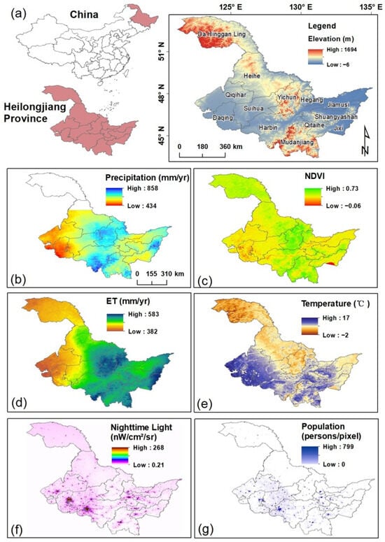
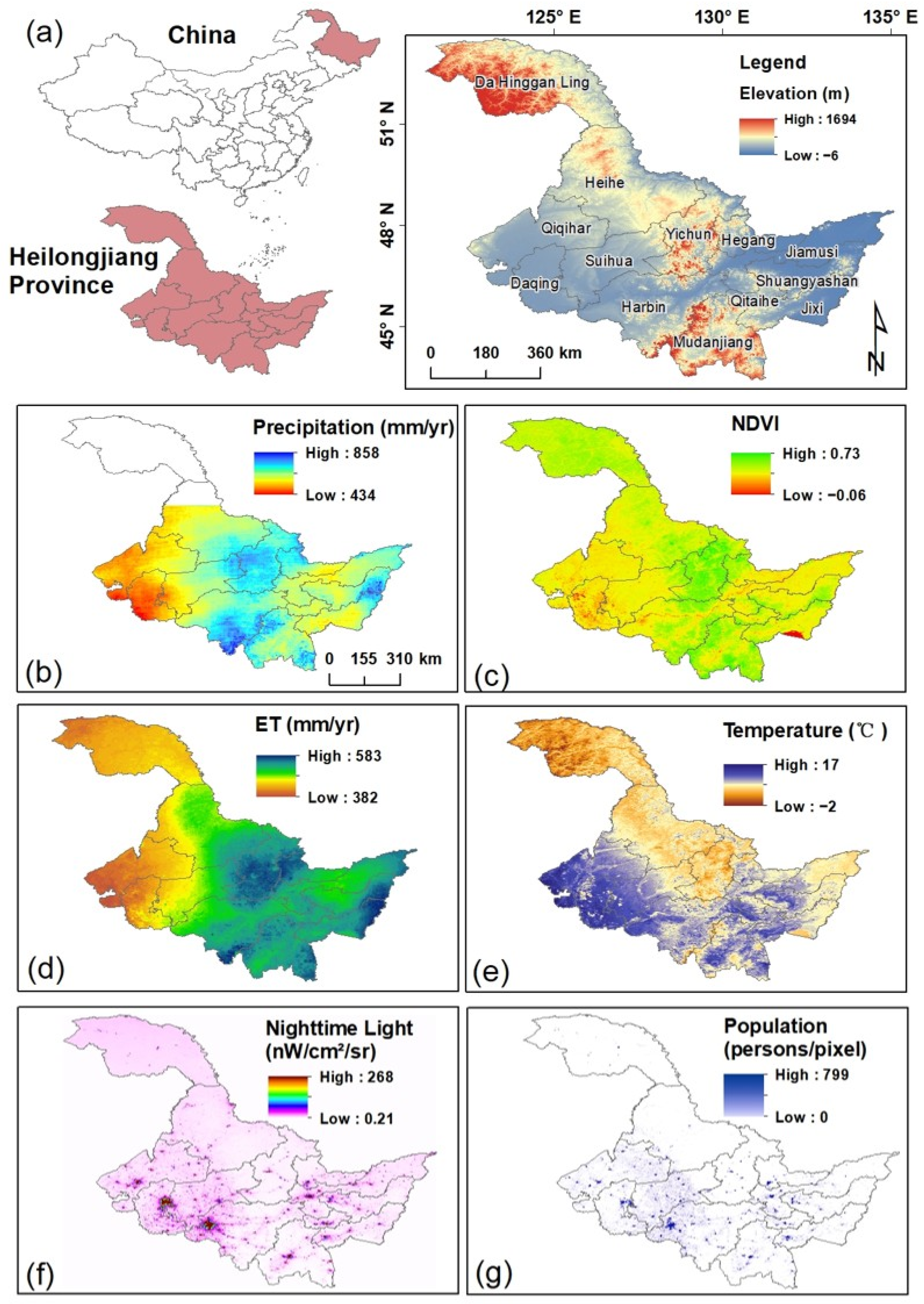
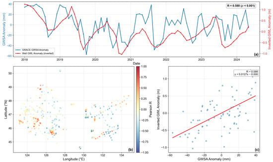
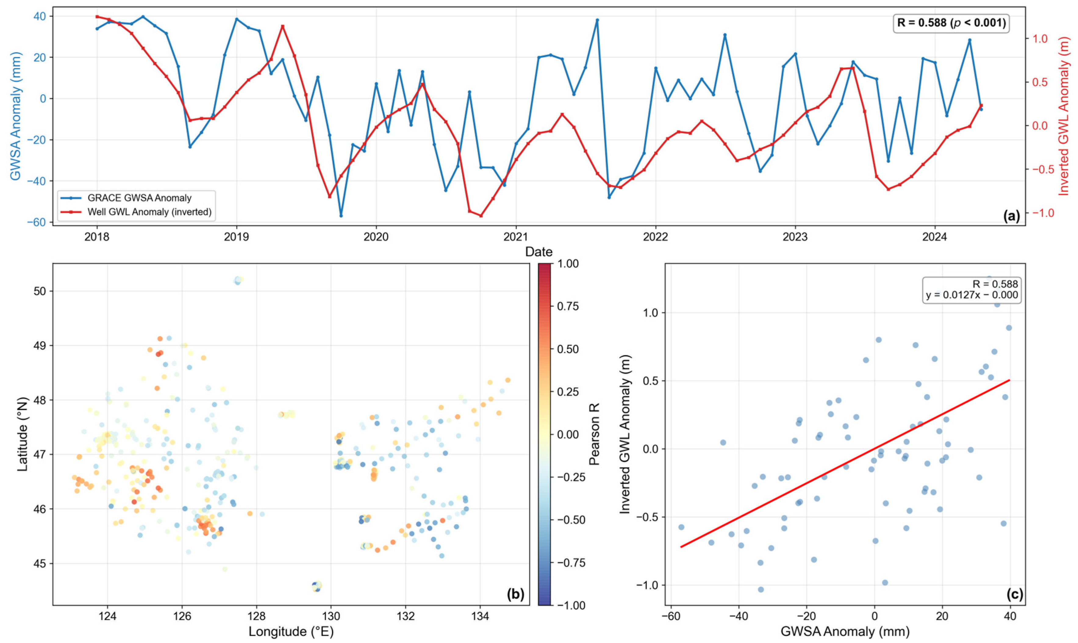
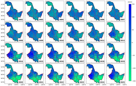
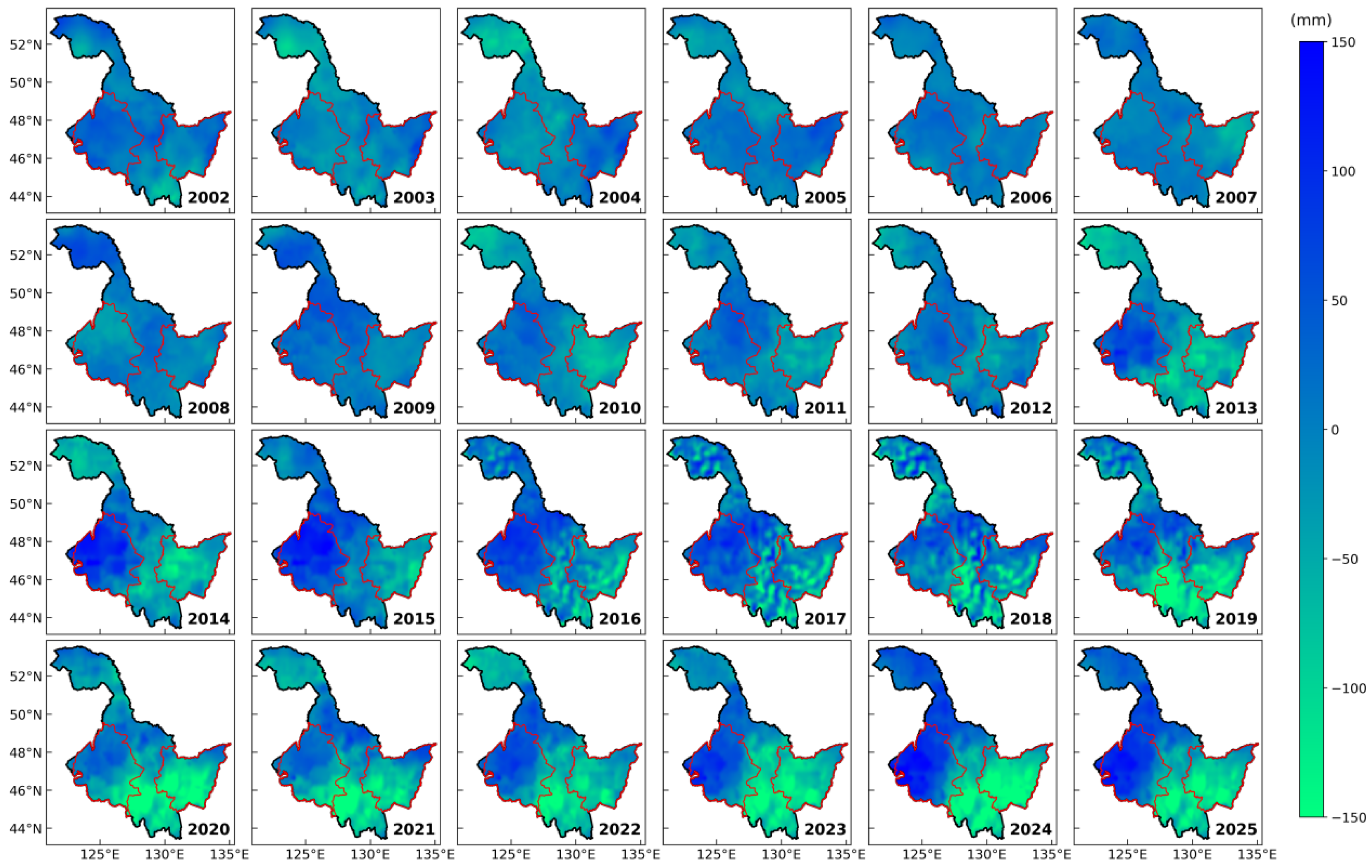
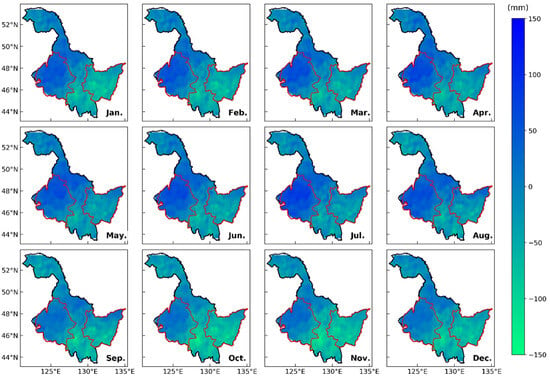
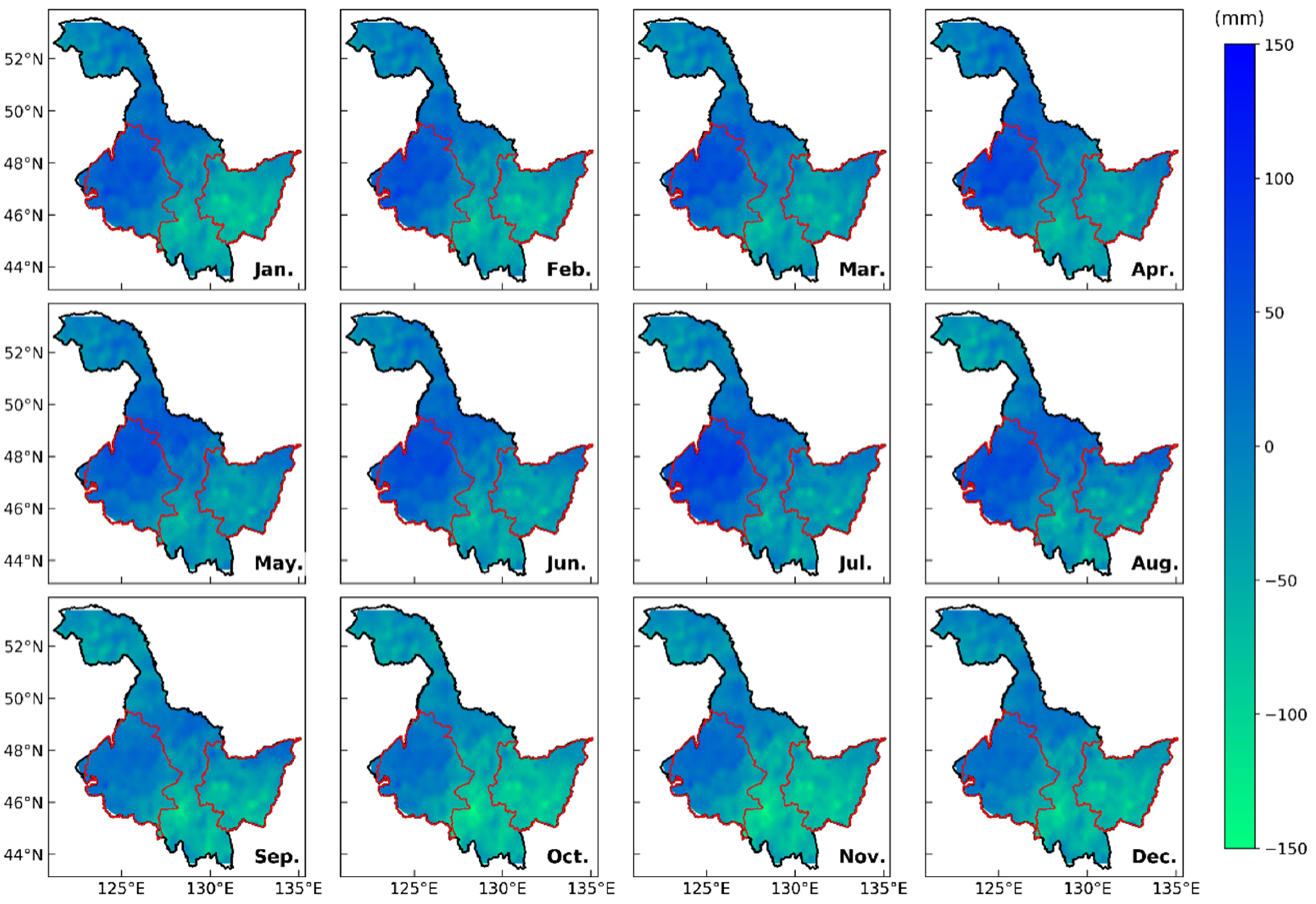
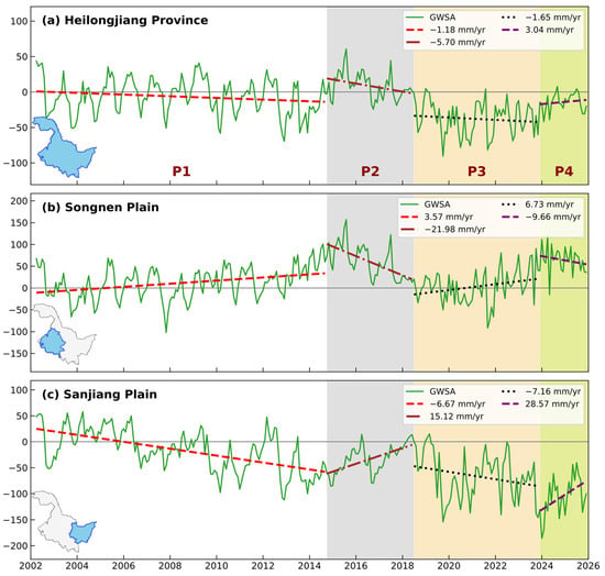
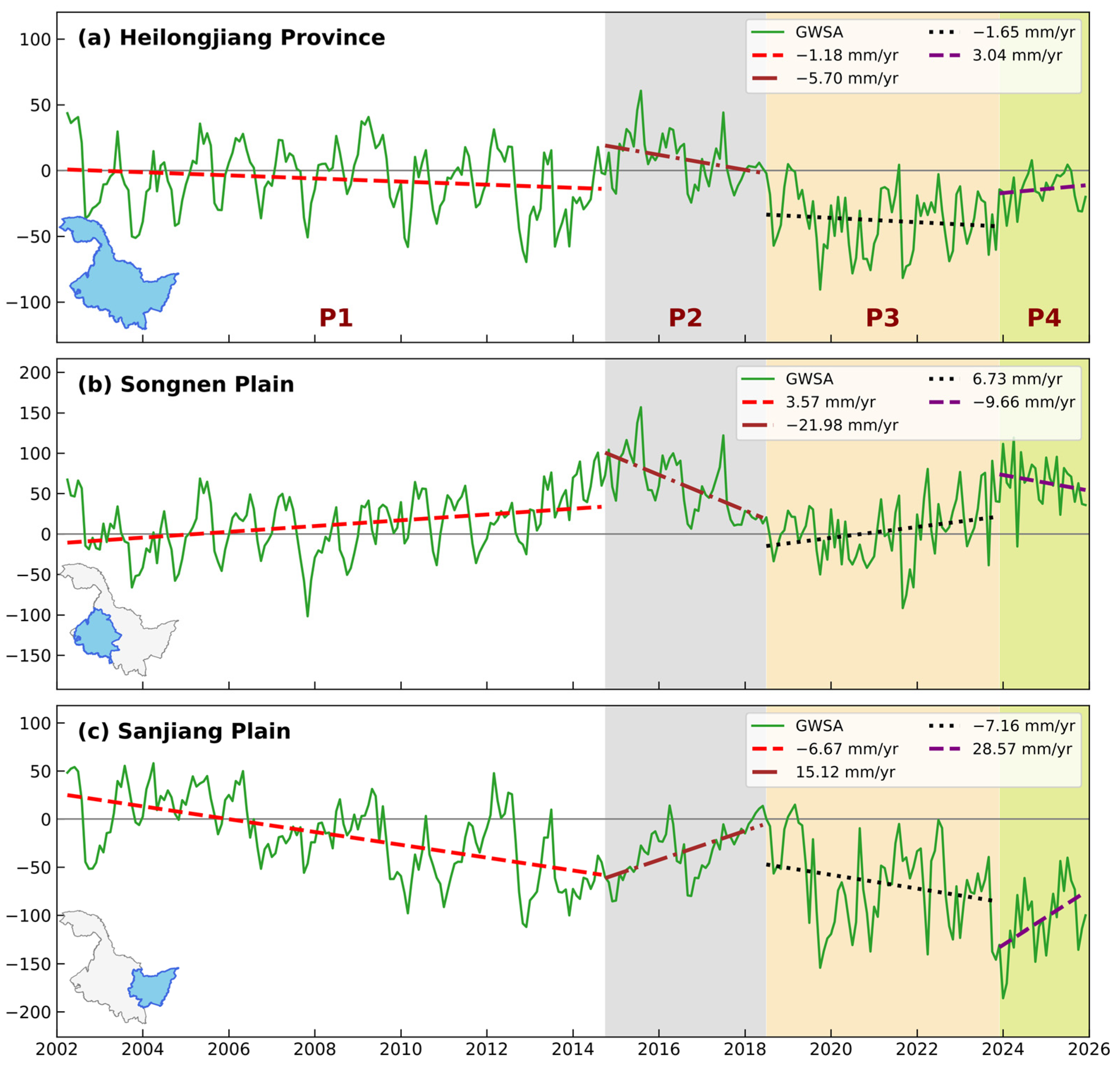
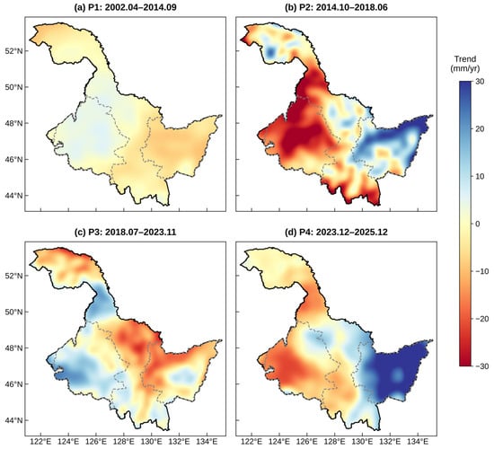
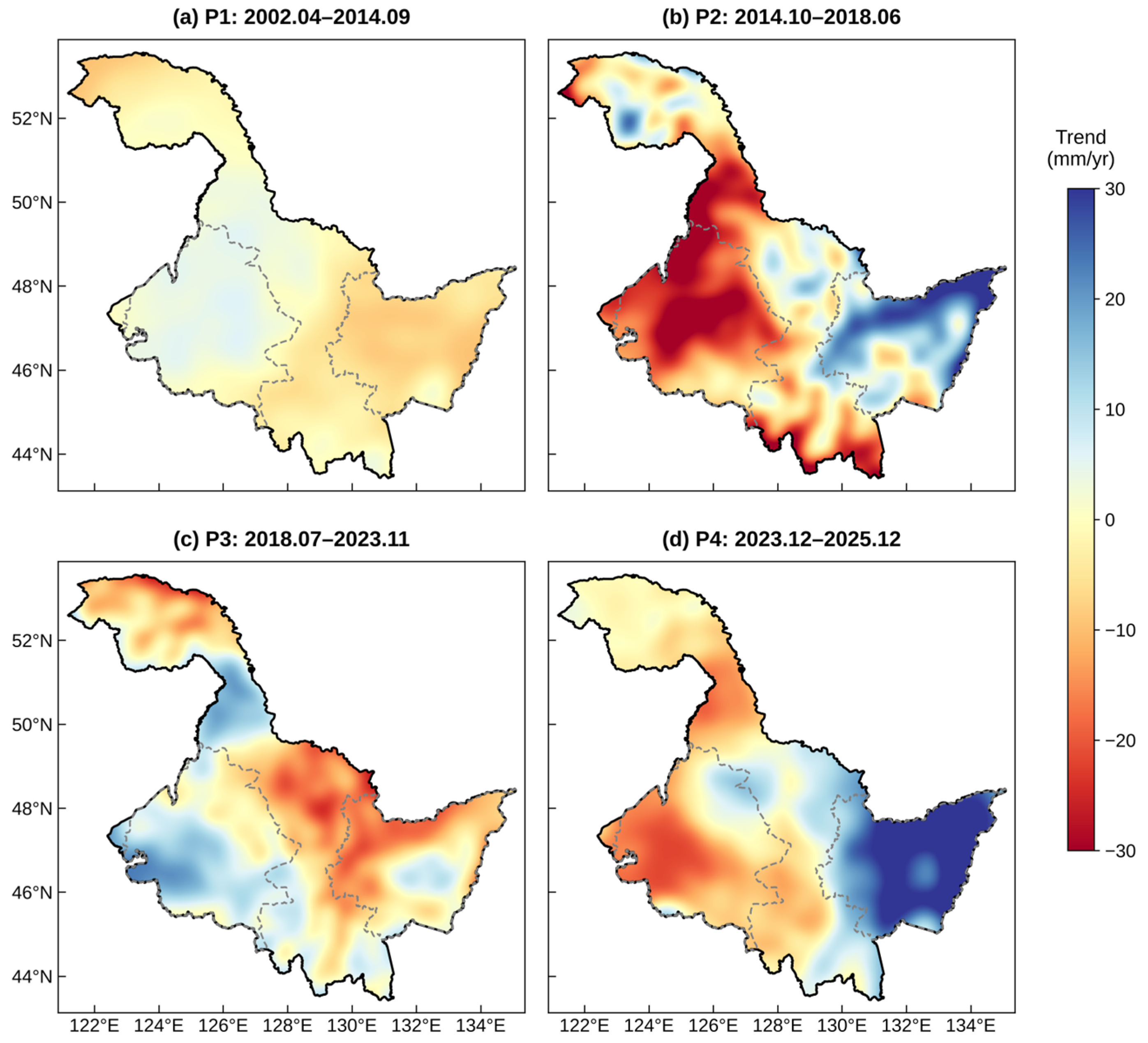
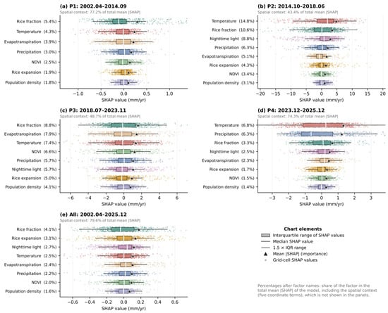
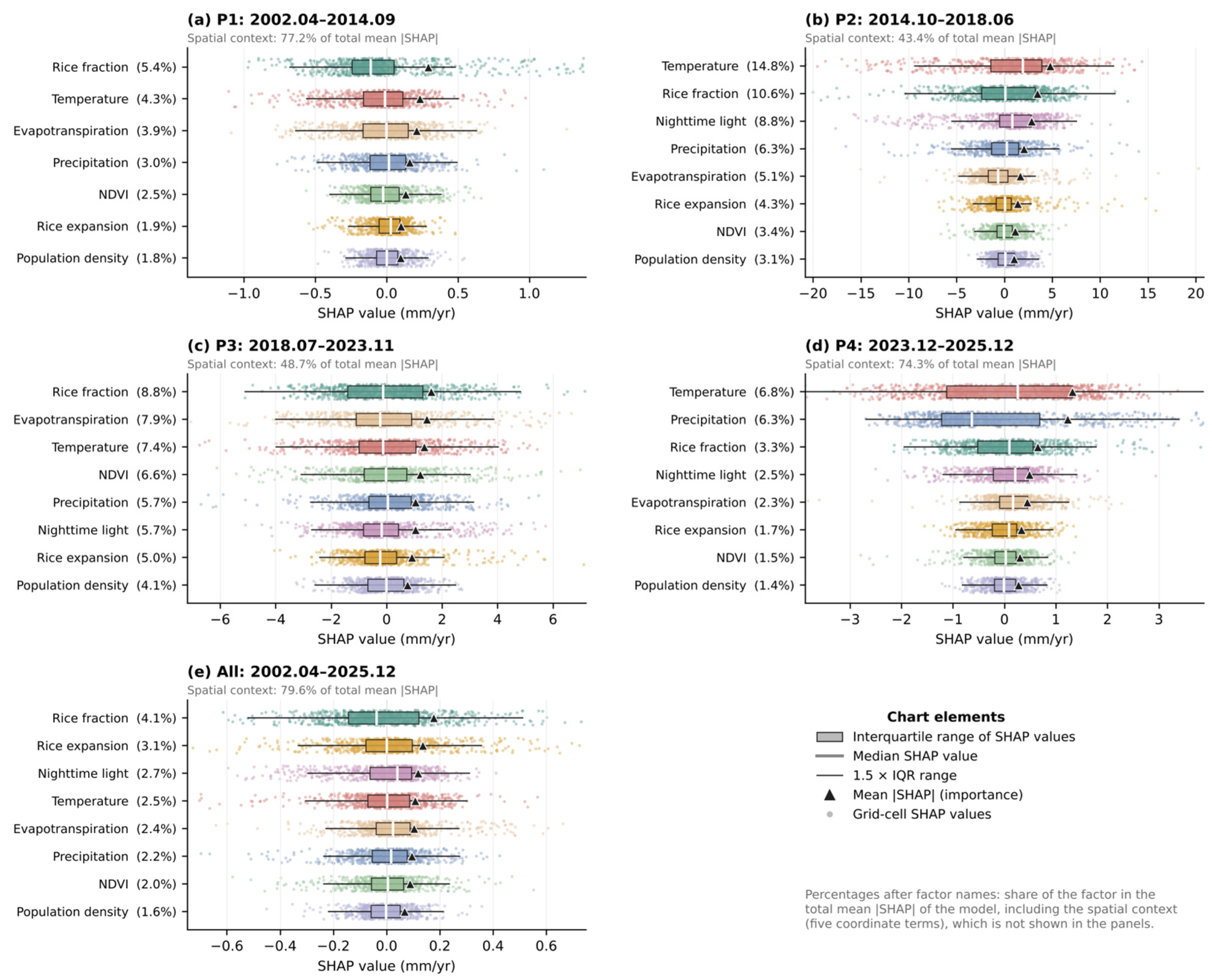
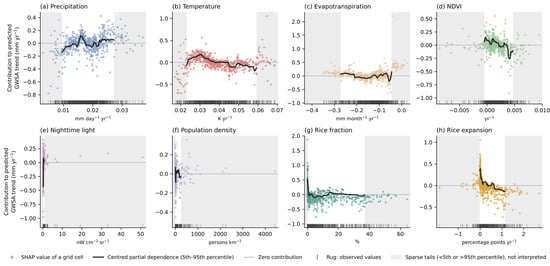
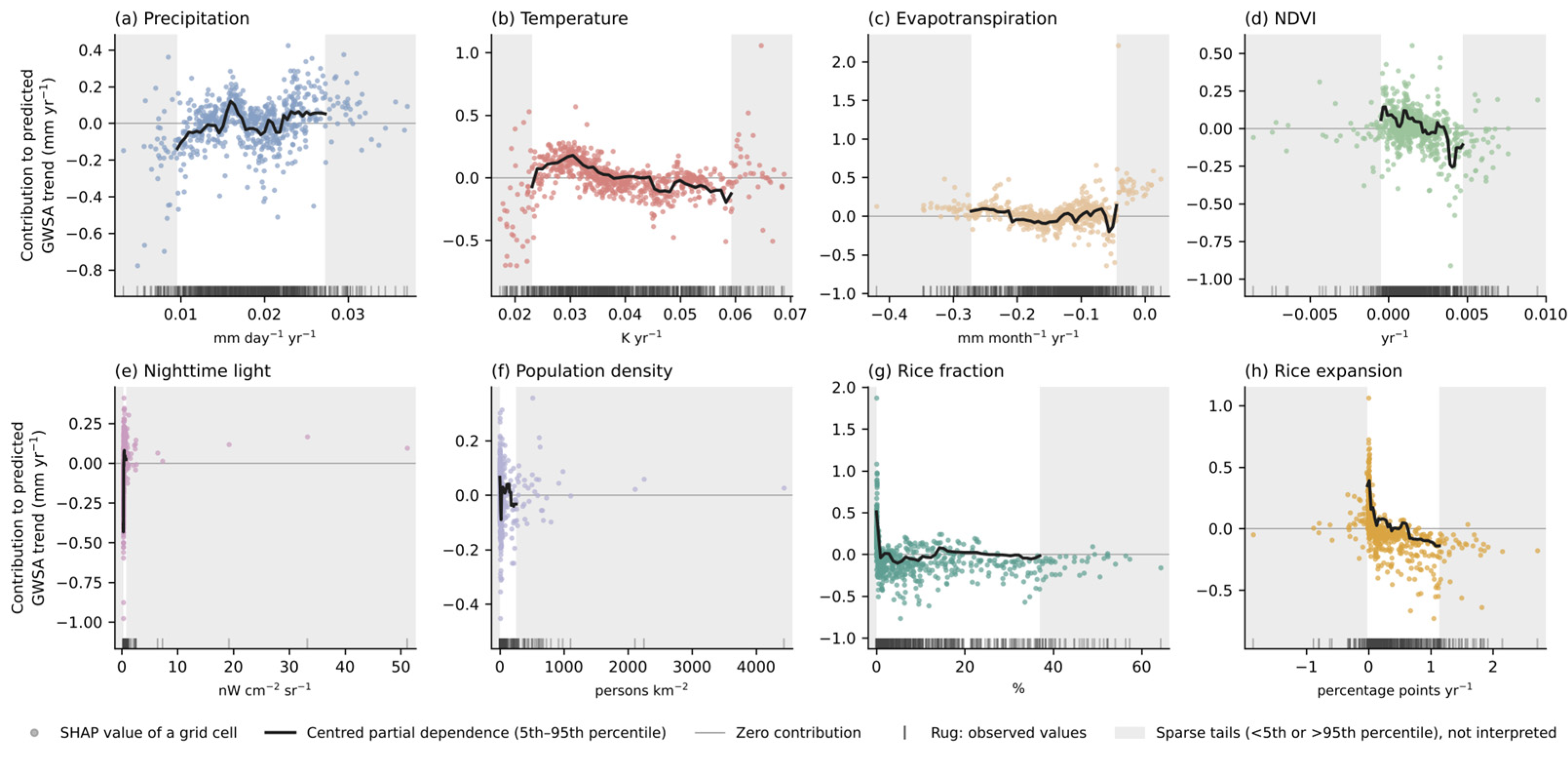
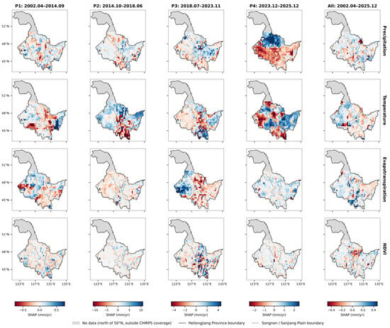
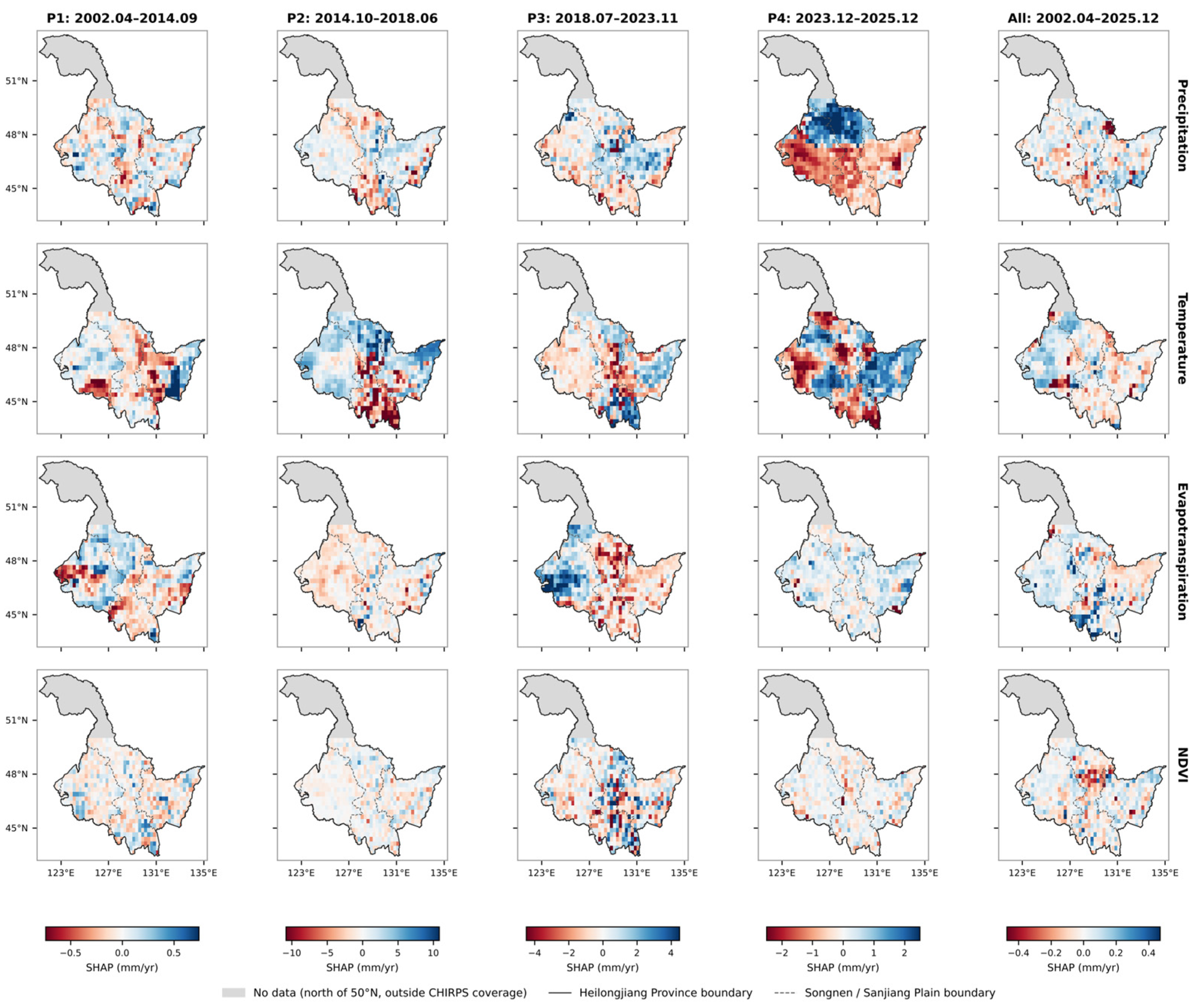
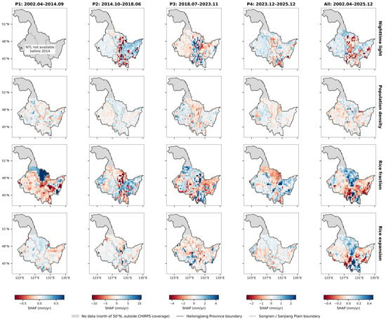
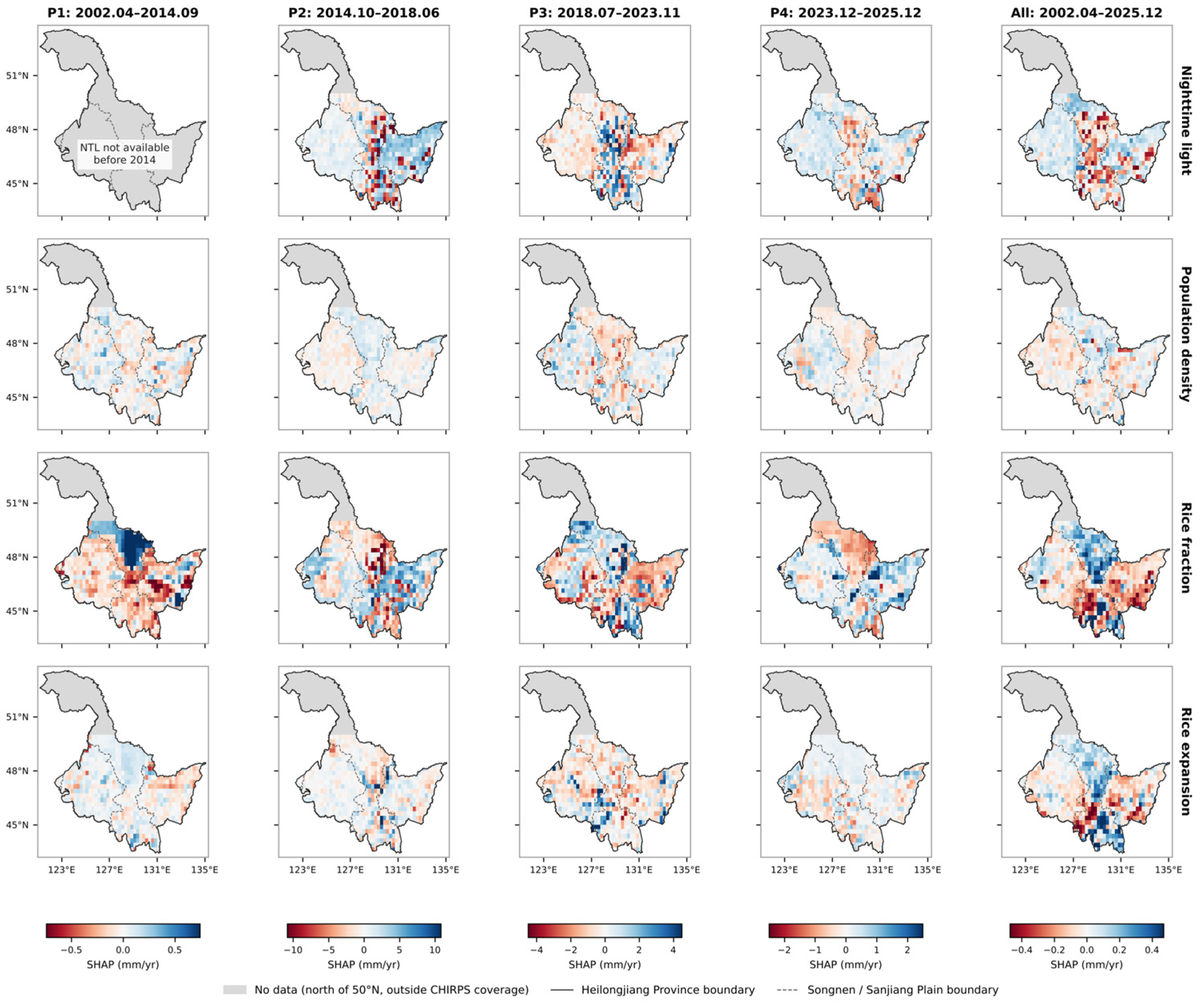
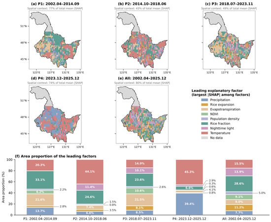
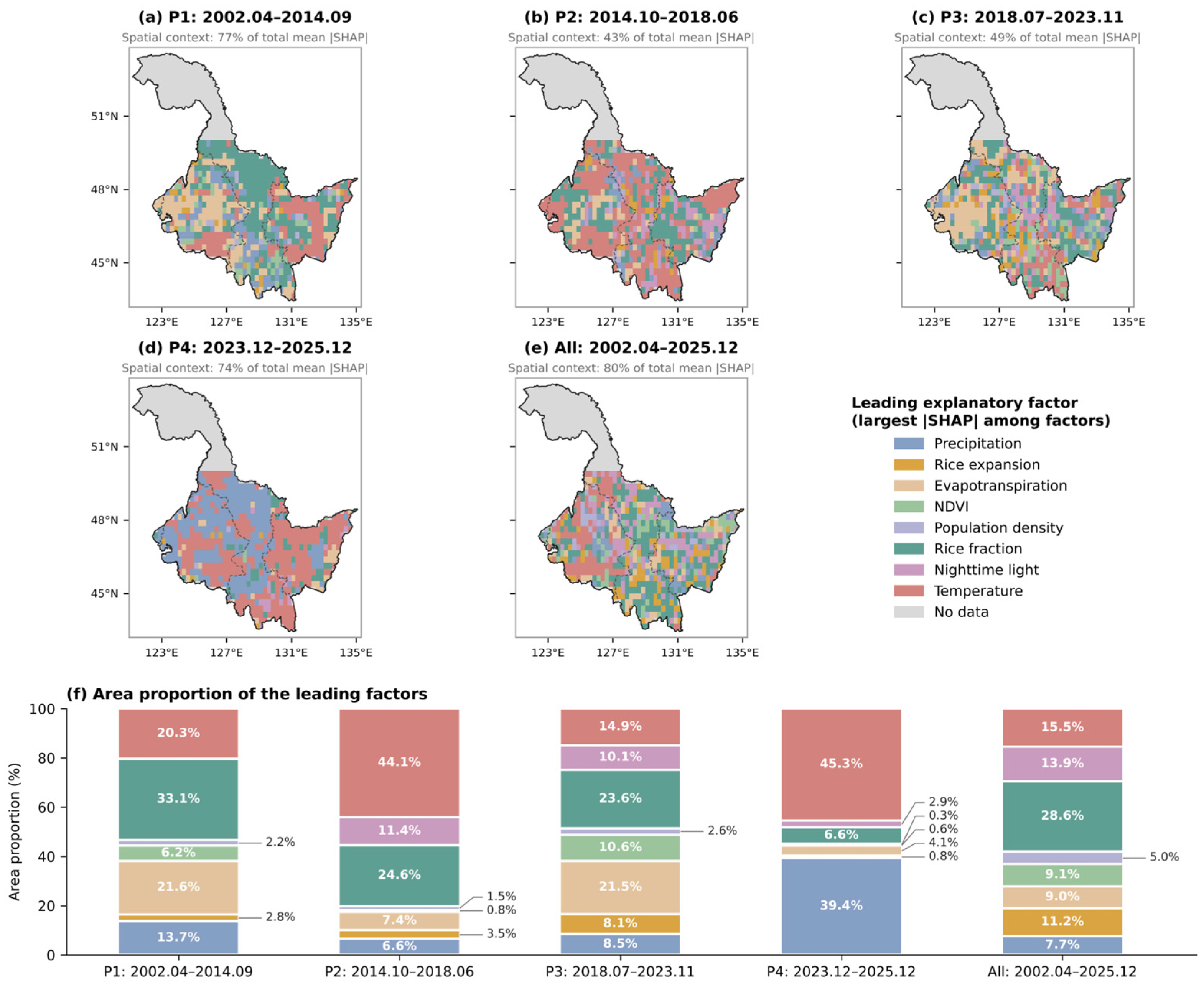

Disclaimer/Publisher’s Note: The statements, opinions and data contained in all publications are solely those of the individual author(s) and contributor(s) and not of MDPI and/or the editor(s). MDPI and/or the editor(s) disclaim responsibility for any injury to people or property resulting from any ideas, methods, instructions or products referred to in the content. |
© 2026 by the authors. Licensee MDPI, Basel, Switzerland. This article is an open access article distributed under the terms and conditions of the Creative Commons Attribution (CC BY) license.