


Abstract
Statistical outlier detection is routine preprocessing for high-frequency water-quality records, but extreme values are of two kinds: technical anomalies and the response to short-term hydrological events. This study asks how that choice affects a total phosphorus (TP) virtual sensor and the information retained. The interquartile range (IQR), Z-score, robust Mahalanobis distance and Isolation Forest were compared with a baseline without statistical outlier removal on 17,059 hourly observations from a Hoeincheon watershed station, Republic of Korea, with thresholds fitted on the training period only and Random Forest and Gradient Boosting scored on a common test set. Removal rates ranged from 0.93% to 20.53%, with no monotonic relation to performance. The Z-score, removing 2.88%, produced the lowest error of the five conditions in this evaluation period for both models; after adjustment for multiple comparisons this reduction was significant for Gradient Boosting only. IQR, removing 20.53%, produced the highest error and removed 98.01% of the rainfall-influenced high-concentration observations. Those observations are both the examples needed to predict elevated TP and the intervals carrying the event structure, so discarding them degraded prediction and fragmented the series together. Preprocessing should therefore be assessed against event retention and temporal continuity as well as error metrics.
1. Introduction
River water-quality monitoring is essential for identifying various problems and current conditions in river systems, and provides fundamental information for maintaining sustainable use of water resources, aquatic biodiversity, and ecosystem services in good condition [1,2,3,4]. However, conventional water-quality monitoring methods rely on periodic sampling and laboratory analysis, which results in low temporal and spatial resolution and makes it difficult to capture rapidly changing water-quality conditions in real time [5,6,7]. To overcome these limitations, river monitoring using physical sensors has been introduced [8].
Sensors are devices that monitor the surrounding environment and periodically generate signals, and they have been adopted across a wide range of fields, including environmental monitoring [9,10,11,12,13,14]. In river water-quality monitoring, in particular, advances in sensor technology have enabled a transition to continuous and real-time monitoring systems [15]. Such sensor-based river monitoring allows the measurement of various water-quality variables at high frequency and is used to characterize the spatiotemporal variability of river water quality in detail [16].
However, these physical sensors have limitations in accurate measurement due to issues such as unstable installation and calibration, signal noise, and malfunction [17,18,19,20,21,22]. As a way to overcome these limitations, artificial intelligence (AI)-based virtual sensor technologies have recently been introduced in the field of water-quality monitoring. AI developed from rule-based automatic judgment [23] into an intelligent technology that learns from diverse data and recognizes patterns, a shift driven by the availability of big data from the 2000s onward [24]. Throughout this development, sensors have served as the key tools producing the large volumes of data that AI training requires, so that the two technologies have advanced in a mutually complementary manner [25,26,27,28].
AI-based virtual sensors are used as a new approach to overcoming the limitations of physical sensors [29,30,31]. A representative example is data-driven models that link multi-parameter data acquired from sensors with virtual sensors to predict variables that are difficult to measure directly by physical sensors [32,33,34,35,36]. Nam et al. [37] predicted total nitrogen (T-N) in rivers by reflecting spatial characteristics of the watershed and using measurements of dissolved oxygen (DO), pH, electrical conductivity (EC), water temperature (WT), chlorophyll-a (Chl-a), and nitrate nitrogen (NO3-N) at each river point. Harrison et al. [6] developed models to predict river nitrogen and phosphorus concentrations using high-frequency sensor data (WT, EC, turbidity, pH, fDOM (fluorescent dissolved organic matter), water pressure, and soil moisture). In this way, sensor-measured variables are used as surrogate variables, and high-frequency measurement data are used as key input data for AI training. Through this, applications such as real-time prediction and pollution source tracking are being implemented, and the integration of AI and sensors provides the foundation for data-driven intelligent river management [8,38,39].
However, high-frequency sensor-based water-quality data inherently contain various uncertainties and noise, and outliers can occur due to sensor malfunctions and external environmental factors [40,41,42]. Existing studies on outlier detection in water-quality and environmental data have mainly relied on labeling based on expert judgment at the watershed or site scale to classify anomaly types [43,44,45]. Although such labeling-based anomaly detection provides detailed diagnostic information, it is impossible to manually inspect all data in high-frequency, large-scale sensor datasets, and data patterns that differ from historical behavior may occur under climate change and environmental change, which leads to limitations in scalability. For effective management of rivers and watersheds and to enhance the applicability of AI-based virtual sensors, producing and collecting high-quality data is of utmost importance. Data containing erroneous measurements can lead to errors in diagnosing river and watershed conditions, and even when advanced prediction models are applied, reliability and accuracy are limited. Data-driven intelligent river management requires systematic and reproducible procedures for identifying and handling outliers [46,47,48].
Various techniques have been applied for outlier detection to produce high-quality data. Methods such as Z-score and interquartile range (IQR) have been mainly used to detect outliers in univariate data [49]. Jeong et al. [50] reported that IQR-based outlier detection shows relatively high stability and accuracy even for non-normal distributions and remains robust under conditions with up to 30% outliers. Although such approaches have the advantage of detecting outliers based on the statistical distribution of individual water-quality variables, actual water-quality changes arise from interactions and coupled patterns among multiple variables, so single-variable-based methods alone are limited in effectively distinguishing complex environmental variability from sensor anomalies.
Robinson et al. [51] showed, for correlated water-quality data, that univariate outlier detection methods may miss true outliers or misclassify normal observations as outliers, and emphasized the need for multivariate approaches that incorporate the correlation and covariance structure among variables. Alameddine et al. [52] compared three robust multivariate outlier detection methods—the Minimum Covariance Determinant (MCD), the Minimum Volume Ellipsoid (MVE) and M-estimators—using national lake water-quality data. MVE flagged the largest number of outliers, whereas MCD was the most conservative, and the conventional Mahalanobis distance, which relies on the sample mean and sample covariance, was shown to leave some outliers undetected in multidimensional water-quality data because those estimates are themselves masked by the extreme values. Environmental monitoring data are marked by non-normality, multivariate structure and strong correlations, so multivariate outlier detection based on robust estimation is required, and the application of detection methods that account for high-dimensional and multivariate data characteristics has been expanding rapidly in recent sensor-based system studies [53]. The Mahalanobis-distance-based multivariate outlier detection method, which accounts for covariance structures among variables, has been widely used and evaluated as effective for early identification of outlier patterns from multivariate data [54,55,56,57].
Although statistical multivariate outlier detection methods have been effectively used in various domains, they have limitations in capturing the complex nonlinear structures and patterns of high-dimensional sensor data. To address these limitations, multivariate outlier detection methods based on machine learning and unsupervised learning have recently gained attention [58], offering more flexible outlier detection in high-dimensional, nonstationary datasets. Liu et al. [59] developed an integrated framework that combines a Bayesian autoregressive prediction model with Isolation Forest and successfully detected outliers in high-frequency water-quality data. Yin et al. [60] combined long short-term memory (LSTM)-based prediction errors with Isolation Forest to detect sudden inflow events in mining areas at an early stage. These studies demonstrate that multivariate outlier detection methods based on machine learning and unsupervised learning provide effective approaches for outlier detection by capturing nonlinear interactions and multidimensional variability among variables. In fields where high-dimensional measurement data are used, machine-learning-based outlier detection has been applied to improve data quality and identify abnormal patterns [61,62,63].
As the use of high-frequency sensor data in river water-quality monitoring expands, data quality control becomes a critical factor that determines the performance of prediction models and the reliability of intelligent river management. In particular, outliers can act as noise during the training of data-driven models, so detecting and handling them is an important part of data preparation. Not all extreme values in high-frequency water-quality records are sensor errors, however: some are the water-quality response to short-term hydrological events such as rainfall and runoff [41,47]. Statistical outlier detection operates only on the distribution of the observed values and cannot distinguish between the two. However, many existing studies have focused on the application and performance evaluation of individual outlier detection methods, and relatively few studies have systematically compared and analyzed how different outlier detection methods affect the performance of subsequent prediction models.
This study applies univariate methods (IQR and Z-score) and multivariate methods (the robust Mahalanobis distance and the Isolation Forest) to detect and remove outliers, and subsequently develops virtual sensor models based on each processed dataset. By doing so, the study aims to quantitatively evaluate how different outlier detection methods influence data quality and the performance of prediction models.
2. Materials and Methods
This study established an analytical framework to evaluate the effects of outlier detection methods on total phosphorus (TP) virtual sensing in high-frequency water-quality sensor data. The framework was designed to assess outlier detection not only as a preprocessing step for improving prediction performance, but also in terms of its effects on prediction performance, data removal, temporal continuity, and the retention of rainfall-influenced high-TP and high-turbidity observations. The overall workflow is illustrated in Figure 1. The analysis first applied physical quality control to remove physically implausible sensor values, after which the data were divided chronologically into training and test sets. Outlier detection thresholds and detectors were estimated using the training data only, and all methods operated on the common input variable set defined in Section 2.1. IQR, Z-score, Robust Mahalanobis and Isolation Forest were applied as outlier detection methods, and the Raw dataset without statistical outlier removal was used as a baseline. The training datasets generated by each method were used to train Random Forest and Gradient Boosting TP virtual sensing models, and all models were evaluated using the same common test set. Finally, each method was compared using prediction performance, removal rate, temporal gaps, changes in lag-1 autocorrelation, and rainfall-influenced event retention.
Figure 1.
Analytical workflow for evaluating the effects of outlier detection on TP virtual sensing performance, temporal continuity, and rainfall-influenced event retention in high-frequency water-quality sensor data.
2.1. Study Area, Data Collection, and Preprocessing
The study area is a water-quality monitoring station located in the Hoeincheon watershed upstream of the Daecheong Dam in central South Korea, and this station is operated by the Korea Water Resources Corporation (K-water) (Figure 2). The Daecheong Dam is a major water resource facility that supplies domestic, agricultural, and industrial water, and it plays a critical role in watershed-scale water-quality management. Hoeincheon is a small- to medium-sized tributary of the Geum River system, flowing through agricultural and rural areas before joining the main channel of the Geum River.
Figure 2.
Location of the Hoeincheon study area and water-quality monitoring station.
South Korea has a temperate monsoon climate characterized by distinct wet and dry seasons, with rainfall concentrated in the summer [64]. As a result, both flow and water-quality characteristics exhibit strong seasonal variability, and changes in rainfall and runoff conditions are major drivers of short-term variability in river water-quality parameters. In addition, the Hoeincheon watershed contains agricultural land and partially urbanized areas, creating a mixed water-quality environment influenced by both non-point and point pollution sources. These watershed characteristics increase the likelihood of abrupt water-quality changes and environmental events in high-frequency monitoring data.
This study used high-frequency sensor records at an hourly resolution from the Hoeincheon water-quality monitoring station between January 2023 and December 2024. Seven variables were used in the analysis: water temperature (TEMP), electrical conductivity (COND), turbidity (TURBIDITY), dissolved oxygen (DO), pH, total phosphorus (TP) and rainfall. These are the parameters routinely measured by the automatic monitoring system operated at this station, and together they represent the physicochemical state of the stream and the mobilization of pollutants during rainfall-driven runoff. TEMP, COND, TURBIDITY, DO and pH are measured with a YSI EXO2 multiparameter sonde (YSI Inc., Yellow springs, OH, USA) and TP with a RoboChem A4-TP analyzer (Centennial Technology, Uiwang City, Republic of Korea); the instruments are calibrated at the weekly routine inspection of the station. Rainfall is measured with a rain gauge and is the amount recorded for each hourly interval (mm). The instruments, the calibration interval and the precipitation measurement are listed in Table S1c.
Each variable serves a distinct role in the analysis. TEMP, COND, TURBIDITY, DO and pH constitute the common input set used by every outlier detection method and by the TP virtual sensing models; operating all methods in an identical feature space ensures that differences in performance reflect the detection algorithm. TP was adopted as the prediction target because it governs eutrophication risk and treatment requirements in the reservoir downstream and is a direct object of management in this catchment, and because it responds sharply to rainfall events, which makes it well suited to assessing how outlier detection affects a record. As the target, TP was excluded from the outlier detection inputs, so that information on the target variable does not enter the preprocessing step. Rainfall was used neither as a model predictor nor as a detection input; it served only as a diagnostic variable, used to define rainfall-influenced periods and to evaluate how well high-TP and high-turbidity observations within those periods were retained by each method. The association between rainfall and the water-quality variables was assessed with Spearman rank cross-correlation at lags of 0 to 48 h, with the Mann–Whitney U test comparing rainfall-influenced periods with the remainder of the record, and with a binomial test of whether the upper 5% of TP and turbidity occur within rainfall-influenced periods more often than the share of the record those periods occupy.
A total of 17,545 hourly observations on the exact hour were available for the study period, and the preprocessing described below was applied to them. First, a cluster of 48 observations with TP ≥ 4 mg/L was removed. These observations are disjoint from the rest of the record and do not form its upper tail: the highest TP value among the remaining observations is 0.585 mg/L, the cluster ranges from 4.561 to 9.406 mg/L, and no observation falls between these two values, so that any threshold within that interval isolates the same 48 records. The cluster is confined in time, occurring between 22 and 26 November 2024 in six runs of consecutive hours of which the longest lasts 20 h, and 47 of the 48 records report zero rainfall for the hour in which they occur. The five sensor variables remain within their usual ranges during these hours, so the anomaly is confined to the TP series; Table S3 reports how the detection criteria evaluated in this study behave with respect to this cluster.
All 48 observations belong to the test period, so their removal leaves the training data and every detection threshold unchanged. This screening is a data-integrity step applied before the four detection criteria are introduced and is not one of the distribution-based criteria evaluated here. This cluster lies outside the concentration range on which the four detection criteria are compared, and it is separated from that range by a gap in which no observation falls, so it is set aside before the comparison. Whether these observations are measurement errors was not determined, and the analysis below is reported for the 17,059 observations that remain. Table S3 reports the cluster in detail and Table S4 the results obtained when it is retained, which leaves the ordering of the five conditions within each model unchanged.
Physical quality control was then applied to remove physically implausible sensor readings, using three rules: records containing a zero value in a non-temperature sensor variable (COND, TURBIDITY, DO or pH) were treated as sensor no-response and removed (326 records); negative turbidity values were removed (111 records); and a single record of 1815 mm hourly rainfall was removed, a value exceeding the highest hourly rainfall ever recorded in Korea by more than an order of magnitude. A water temperature of 0 °C is physically possible and was retained. After this preprocessing, 17,059 observations remained and were used in the analysis (Table 1).
Table 1.
Descriptive statistics of the final high-frequency water-quality dataset. SD, standard deviation.
The final analysis dataset was divided chronologically into a training and a test period for TP virtual sensing model development and evaluation. The first 80% of the records (n = 13,647, up to 9 August 2024 19:00) were assigned to the training period and the remaining 20% (n = 3412) to the test period, thereby preserving the temporal structure of the observations. To prevent test-period information from influencing the outlier detection criteria, all thresholds and detectors were estimated from the training-period data only. The resulting criteria were then evaluated over the whole screened record, but observations were removed only from the data used to fit the prediction models; no observation was removed from the test period. All preprocessing methods are evaluated on a single common test set containing identical observations. Observations with TP = 0, which correspond to values below the detection limit, were excluded from model fitting and evaluation, leaving 3367 test observations for the performance comparison.
Holding the test period fixed isolates the effect of cleaning the training data, which is the question addressed here: if each condition were also evaluated on its own cleaned test set, the conditions would be scored on different observations and the comparison would confound the effect of preprocessing with differences between the evaluation sets. An operational pipeline would apply the same preprocessing to incoming data, so the values reported here describe the effect of the training data on the fitted model rather than the end-to-end performance of such a pipeline; this distinction is revisited in Section 4.
Table 1 presents the descriptive statistics of the final analysis dataset and summarizes the preprocessing procedure. High-frequency water-quality data can exhibit abrupt variability due to rainfall, runoff, sensor conditions, and changes in pollution-source dynamics within the watershed, so statistically extreme values do not always indicate sensor errors. Accordingly, this study distinguished physically implausible values from statistical anomaly candidates and evaluated their effects on prediction performance, data removal, temporal continuity, and rainfall-influenced event retention in the subsequent analysis.
2.2. Outlier Detection Methods
Outlier detection methods were applied to the high-frequency water-quality dataset after physical quality control and preprocessing. The Raw dataset without statistical outlier removal was used as the baseline, and IQR, Z-score, Robust Mahalanobis distance, and Isolation Forest were applied as outlier detection methods. The common input variables defined in Section 2.1 were used for outlier detection, and the main settings of each method are summarized in Table 2.
Table 2.
Settings of the outlier detection methods.
A distinction is maintained throughout between a measurement error and a statistical outlier. A measurement error is an observation that does not represent the state of the water body, such as a sensor no-response or a physically impossible value; observations of this kind were removed deterministically at the physical quality control stage described in Section 2.1. A statistical outlier is an observation that lies far from the bulk of the observed distribution, which is a property of the distribution, not evidence of a fault: in a stream under rainfall influence, the largest turbidity and TP values are produced by the hydrological response itself, so that they are outliers in the distributional sense without necessarily being measurement errors. The four criteria compared in this section detect statistical outliers, and in the absence of independent reference measurements, it cannot be established which of the flagged observations are errors. They are described as detected outliers and not as detected errors, and the consequences of treating the two as equivalent are examined in Section 3.4 and Section 4.
2.2.1. Univariate-Based Outlier Detection—IQR and Z-Score
IQR and Z-score were applied as univariate outlier detection methods based on the distributional characteristics of individual variables. The IQR is a non-parametric method based on Tukey’s boxplot rule [65] and is defined as the difference between the first quartile (Q1) and the third quartile (Q3), representing the variability of the central 50% of the data. It is also known as a robust statistical measure that provides stable estimates even in the presence of outliers or non-normal distributional shapes [66]. Owing to these characteristics, the IQR can be used for preprocessing environmental monitoring sensor data that may contain skewed distributions, irregular distributional forms, or unexpected extreme values. The IQR is calculated as shown in Equation (1).
where IQR represents the range of the central 50% of the data, Q3 denotes the third quartile (75th percentile), and Q1 denotes the first quartile (25th percentile).
Outliers are then defined as observations that fall outside the thresholds given in Equation (2).
where x represents an individual sensor observation, and 1.5 × IQR corresponds to Tukey’s fences used as the criterion for outlier detection. In this study, the thresholds in Equation (2) were calculated using the training-period data and then used to classify observations outside these thresholds as outliers.
The Z-score represents the standardized distance of an observation from the mean of a variable in units of standard deviation. The Z-score is calculated as shown in Equation (3).
where x represents an individual sensor observation, μ is the mean calculated from the training-period data, σ is the standard deviation calculated from the training-period data, and Z is the standardized value of x. In this study, observations with an absolute Z-score greater than 3 were classified as outliers according to Equation (4), where |Z| denotes the absolute value of the Z-score.
The Z-score is simple to calculate and interpret, but it can be influenced by skewed distributions or extreme values because it relies on the mean and standard deviation. IQR and Z-score were applied together as basic univariate outlier detection methods to compare how differences in univariate criteria affect TP virtual sensing performance and data preservation.
2.2.2. Multivariate Distance-Based Outlier Detection—Robust Mahalanobis Distance
In environments where multiple variables are measured simultaneously, these variables often exhibit correlated variations, which makes it difficult to identify outliers using univariate approaches that evaluate each variable independently. In particular, for river water quality, where diverse variables are interlinked and form covariance structures, approaches based on single-variable criteria are limited. Such approaches cannot sufficiently capture complex variation patterns and carry the risk of missing true outliers or misclassifying normal data as outliers.
Mahalanobis distance (MD) is a distance metric used to measure the distance between two points in a multivariate space and is conceptually similar to the Euclidean distance. Euclidean distance is the most basic method for computing the straight-line distance between two points in a multivariate space, but it does not account for correlations among variables and can lead to misleading evaluations when detecting multivariate outliers. In contrast, MD is a useful distance measure for identifying outliers because it incorporates the correlations among variables [67,68,69,70]. Since MD takes into account the correlations and covariance structures among variables, it can represent the data structure more accurately than the Euclidean distance when the data distribution around the mean is non-spherical or elliptical. The Mahalanobis distance is defined as shown in Equation (5):
where MDi represents the Mahalanobis distance of the i-th observation from the mean vector in the multivariate space, and larger values indicate a higher likelihood of being an outlier. Here, xi denotes the multivariate observation vector, μ is the mean vector, and (xi − μ) represents the deviation vector. Σ is the covariance matrix describing the relationships among variables, and Σ−1 is its inverse, which accounts for differences in scale and correlation. The term (xi − μ)ᵀ Σ−1 (xi − μ) represents the covariance-adjusted squared distance.
The Mahalanobis distance depends on the mean vector and the covariance matrix, and both quantities are themselves sensitive to the extreme values that the method is intended to detect. The distance itself is a quadratic form and does not depend on a distributional model, but the chi-square reference distribution ordinarily used to turn the squared distance into an outlier criterion follows from multivariate normality of the input variables. That assumption was examined for the variables used in this study. All five variables deviated significantly from normality (D’Agostino–Pearson omnibus test, p < 0.001), and several were strongly right-skewed, with a skewness of 16.30 for turbidity and 5.95 for electrical conductivity. When the sample mean and the sample covariance are used with such distributions, a small number of extreme observations inflates the covariance estimate and masks the very observations that should be flagged.
For this reason the mean vector and the covariance matrix in Equation (5) were estimated with the Minimum Covariance Determinant (MCD) estimator [71], which identifies the subset of observations with the smallest covariance determinant and derives location and scatter from that subset, so that the estimates are not distorted by a limited number of extreme observations. Both estimates were obtained from the training-period data only. The outlier threshold was defined as the mean robust distance of the training period plus three standard deviations, corresponding to 149.54 for this dataset, and observations exceeding this threshold were classified as outliers. The distribution of these robust distances is itself strongly right-skewed, with a skewness of 15.48. The chi-square quantiles commonly used with this statistic follow from multivariate normality of the input variables, and a D’Agostino test rejects normality for each of the five variables, so that reference distribution rests on an assumption that this record does not satisfy; the empirical quantiles of the robust distances depart from it in the same direction, as reported in the note to Table S1a. Thresholds derived from the chi-square distribution with five degrees of freedom were therefore examined as a sensitivity analysis at α = 0.05, 0.025, 0.01 and 0.001 (Table S1a), and the outcome is reported in Section 3.2 and Section 4.
2.2.3. Nonlinear Multivariate Outlier Detection—Isolation Forest
Environmental and river monitoring data consist of multivariate observations in which multiple water-quality variables are measured simultaneously, and these variables interact to form complex variation patterns. In natural systems such as river water quality, relationships among variables often involve diverse nonlinear interactions. To detect outliers in such multivariate data, a nonlinear multivariate outlier detection method, Isolation Forest (IF), was applied.
IF, proposed by Liu et al. [72], is an unsupervised anomaly detection algorithm that identifies outliers through the process of isolating observations instead of relying on distance- or density-based approaches. The method is based on the assumption that outliers are located in relatively isolated regions of the data space and are therefore more likely to be separated with fewer partitioning steps during the random splitting process. In contrast, normal observations form dense clusters and require many partitioning steps to be separated, resulting in longer path lengths.
Isolation Forest constructs multiple isolation trees (iTrees) by recursively and randomly partitioning the data space and calculates the path length required to isolate each observation. Based on the average path length of an observation, the outlier score is computed as shown in Equation (6).
where E(h(xi)) represents the average path length required to isolate observation xi, and c(n) is a normalization factor corresponding to the average path length for a dataset of size n. The outlier score s(xi, n) ranges between 0 and 1, and values closer to 1 indicate a higher likelihood of the observation being an outlier.
Isolation Forest does not require assumptions about the underlying data distribution and can efficiently detect outliers in high-dimensional multivariate data, which makes it well suited to sensor-based environmental monitoring data. In this study the model was fitted on the training-period data only, using 200 isolation trees (n_estimators = 200), a fixed random seed (random_state = 42) and a contamination parameter of 0.10.
The contamination parameter specifies the expected proportion of outliers and determines how many observations are flagged. The removal rate obtained with Isolation Forest is consequently set by this parameter, and, when a fixed value is used, it is not directly comparable with the data-driven removal rates of the IQR, Z-score and robust Mahalanobis criteria.
The proportion of genuinely erroneous observations is not known a priori for the present record, and no labeled reference set exists against which a particular value could be validated; the value of 0.10 adopted here is the default used by the scikit-learn implementation before version 0.22, not a quantity estimated from this record. The contamination parameter is treated here as a design choice that has to be declared, and the practical difficulty of fixing it is itself one of the findings reported in this study. The sensitivity of the results to this value was examined over the range 0.03 to 0.20, and the method was additionally evaluated under the rule contamination = ‘auto’, which in scikit-learn 1.3.2 follows the threshold of the original Isolation Forest algorithm: the fitted offset is set to −0.5 and an observation is classified as an outlier when its score falls below that value. Under this rule the analyst does not prescribe an outlier fraction, so the resulting removal rate is determined by the distribution of the scores obtained for the record. Removal rates for all of these settings are given in Table S1a and the corresponding results in Table S6.
2.3. Prediction Models and Performance Evaluation
Two prediction models from different algorithmic families were used, so that the effects of outlier detection on TP virtual sensing could be separated from behavior specific to a single algorithm. Random Forest (RF), proposed by Breiman [73], is a bagging-based ensemble that builds multiple decision trees on bootstrap samples and averages their predictions, which reduces model variance and limits overfitting. Gradient Boosting (GB) is a boosting-based ensemble in which trees are fitted sequentially, each tree correcting the residuals of the preceding ones. Bagging and boosting respond differently to noise and to shifts in the data distribution, so agreement between the two models indicates an effect of the preprocessing method, not of the learning algorithm.
Both ensembles learn nonlinear relationships and interactions among variables effectively and have been widely used in environmental and water-quality studies. RF is comparatively robust to noise because predictions are averaged over independently grown trees, whereas GB fits residuals sequentially and is more responsive to the fine structure of the training data, including any structure introduced by outlier removal.
A separate RF model and a separate GB model were fitted for each preprocessing method using the training set produced by that method, and every fitted model was evaluated on the identical common test set defined in Section 2.1. Differences in the reported performance originate from the training data. The settings of both models are given below and are repeated, together with the software versions, in Table S1c of the Supplementary Materials.
Each model was fitted inside a pipeline in which the five predictors were first rescaled to the unit interval by a min-max transformation. For RF, the number of trees, the maximum tree depth and the splitting criterion were selected by an exhaustive grid search over 10, 30, 50, 70 and 90 trees, maximum depths of 10, 30, 50, 70 and 90, and the squared-error and Friedman mean-squared-error criteria, using five-fold cross-validation on the training data of each preprocessing condition. The selected settings were 90 trees under every condition, with a maximum depth of 30 for the raw, Z-score and robust Mahalanobis conditions, 50 for IQR and 70 for Isolation Forest, and the Friedman mean-squared-error criterion for the raw condition and the squared-error criterion for the remaining conditions. For GB, 200 trees, a maximum depth of 3 and a learning rate of 0.05 were used under every condition. The random seed was fixed at 42 throughout, and all remaining parameters retained the default values of scikit-learn 1.3.2.
Model performance was evaluated using the predicted/observed ratio, the mean absolute error (MAE) and the root mean square error (RMSE). The coefficient of determination was not adopted as a primary metric because TP in this catchment is strongly right-skewed and the high-concentration range is sparsely sampled, so that R2 is dominated by a small number of large observations and becomes unstable across the preprocessing methods being compared. The predicted/observed ratio expresses the mean predicted concentration relative to the mean observed concentration and is defined as shown in Equation (7):
where yi is the observed value, ŷi is the predicted value and n is the number of test observations. A ratio of 1 indicates agreement between the mean predicted and mean observed concentrations, whereas values below 1 indicate underestimation and values above 1 indicate overestimation.
The MAE expresses the average magnitude of the prediction error in the units of the target variable and is defined as shown in Equation (8):
where |yi − ŷi| is the absolute error of the i-th observation. Lower values indicate better accuracy, and, unlike the RMSE, the MAE weights all errors equally.
The RMSE evaluates prediction accuracy based on the squared differences between observed and predicted values, and is defined as shown in Equation (9):
where yi and ŷi denote the observed and predicted values, respectively, and n is the total number of observations. RMSE is more sensitive to large errors, and lower values indicate better predictive accuracy.
Because a single chronological split can be sensitive to the period assigned to the test set, the uncertainty of the comparison was additionally assessed using a five-fold TimeSeriesSplit cross-validation in which the outlier detection step was refitted within each training fold. The resulting means and standard deviations are reported in Table S1b. In addition, because every condition is evaluated on the same test observations, the absolute prediction errors obtained under each preprocessing condition were compared pairwise with those of the raw baseline. The paired differences in absolute error are serially correlated, so the difference in mean absolute error was tested with a paired circular moving-block bootstrap of the difference series, using 100,000 resamples and 20,000 for the sensitivity checks. The blocks are contiguous in the order of the retained observations and not in clock time, so a block can span the 27 interruptions of the hourly sequence that fall within the test period; the effect of this was examined by repeating the bootstrap with the blocks confined to uninterrupted stretches. The block length was selected separately for each comparison from the estimated serial dependence of that series by the automatic rule of Politis and White [74], which returned 11 to 141 observations, and each comparison was also repeated at fixed lengths of 6, 12, 24, 48, 72 and 168 observations. Because eight comparisons are made against the same baseline, the bootstrap p-values were adjusted by the Holm procedure. Table S7 reports the settings, the results and their sensitivity to these choices, together with the Wilcoxon signed-rank values obtained on the same pairs, which do not account for the serial dependence and are listed for reference only.
3. Results
3.1. Characteristics of the Water-Quality Dataset
The final dataset used in this study consists of 17,059 hourly observations recorded between January 2023 and December 2024. It comprises the five water-quality variables measured by the multi-parameter sensor—water temperature (TEMP), electrical conductivity (COND), turbidity (TURBIDITY), dissolved oxygen (DO) and pH—together with total phosphorus (TP) as the prediction target and hourly rainfall as an auxiliary variable used only to define rainfall-influenced periods. Descriptive statistics of all variables are given in Table 1. TP had a mean of 0.029 mg/L and a maximum of 0.585 mg/L, and turbidity had a mean of 7.71 NTU and a maximum of 1210 NTU. Both variables are therefore strongly right-skewed, and their upper ranges are represented by comparatively few observations.
Figure 3 shows the temporal variation of the seven variables. TEMP and DO follow clear and mutually inverse seasonal cycles, whereas TP and turbidity remain low over most of the record and rise abruptly at isolated time points. These abrupt rises are concentrated in the summer months and coincide with the rainfall peaks in Figure 3c, which indicates that a substantial part of the extreme values in TP and turbidity is associated with rainfall–runoff processes. COND behaves in the opposite way: it stays close to its median for most of the record and falls sharply during the same rainfall periods, which is the dilution response expected during storm flow.
Figure 3.
Time series of the variables used in this study: (a) total phosphorus (TP), (b) turbidity, (c) rainfall, (d) electrical conductivity (COND), (e) water temperature (TEMP), (f) dissolved oxygen (DO) and (g) pH. Abrupt increases in TP and turbidity and simultaneous decreases in COND coincide with the rainfall peaks shown in panel (c).
The association between rainfall and these abrupt rises was examined statistically. Spearman rank cross-correlations were computed at every integer lag from 0 to 48 h, with each pair matched by timestamp so that a lag of k hours compares the rainfall at t with the response at t + k h. The strongest associations occur approximately 6 h after the rainfall for turbidity (rho = 0.235, 16,626 matched pairs), 9 h after the rainfall for TP (rho = 0.188, 16,597 pairs) and 24 h after the rainfall for electrical conductivity, with the opposite sign (rho = −0.170, 16,901 pairs). One hour of the record carries two logged observations, and the three coefficients are unchanged to three decimal places whether the first, the second or their mean is used for that hour. The hourly observations are themselves autocorrelated and the reported lag is the largest coefficient among 49 candidates, so these coefficients are reported as descriptive measures of association and not as tests of it. The sequence—the mobilization of particulate material recorded by turbidity first, the TP response next and dilution of the dissolved load last—is the order expected of a rainfall–runoff response. The differences between adjacent lags are small, so the individual lag values should not be over-interpreted, but the signs and the ordering are consistent with a delayed water-quality response to rainfall.
The concentrations themselves differ between rainfall-influenced periods and the remainder of the record: the median TP is 0.031 against 0.018 mg/L, the median turbidity 3.24 against 2.41 NTU, and the median conductivity 299.2 against 338.4 µS/cm, the last again in the opposite direction. The timing of the extreme values is the clearest indication: rainfall-influenced periods occupy 28.0% of the record, yet they contain 79.6% of the observations in the upper 5% of TP (682 of 857) and 64.1% of those in the upper 5% of turbidity (547 of 853), against the 28.0% that would be expected if the extreme values fell independently of rainfall. The hourly observations within a single event are not independent of one another, so the group medians and these proportions are reported as descriptive measures of the association. The Mann–Whitney U and binomial tests computed on the hourly observations give p < 0.001 in every case, but they treat those observations as independent and are therefore not used here as evidence that the association is not coincidental. These patterns support a rainfall-associated response, but they do not by themselves exclude sensor error: no independent reference measurements are available, so it cannot be established which of these observations are faults.
The extreme values visible in Figure 3 therefore have two distinct origins. Some are produced by sensor noise or malfunction and carry no information about the state of the river, whereas others are the water-quality response to short-term hydrological events and are physically meaningful. Statistical outlier detection operates only on the distribution of the data and cannot separate the two, so the extent to which each method removes event-related observations is examined in Section 3.2 and Section 3.4.
3.2. Outlier Detection Results
The four statistical outlier detection methods were applied to the 17,059 observations, with all thresholds estimated on the training period only. The resulting removal rates differ by more than an order of magnitude (Table 3). IQR removed 3503 observations (20.53%), Isolation Forest removed 1550 (9.09%), Z-score removed 492 (2.88%) and the robust Mahalanobis distance removed 158 (0.93%). The removal rate of Isolation Forest is fixed by the contamination parameter, so it is a design choice, whereas the rates of the other three methods are determined by the data distribution. Thresholds obtained from the chi-square distribution with five degrees of freedom remove a far larger share of the record than the empirical threshold: 4634 observations (27.16%) at α = 0.001, rising to 6246 (36.61%) at α = 0.05 (Table S1a). None of these four conditions improved on the untreated baseline, and each removed between 797 and 800 of the 803 rainfall-influenced high-concentration observations defined in Section 3.4, leaving a retention of 0.37% to 0.75%. Under the rule contamination = ‘auto’ the removal rate was 10.35% (1766 observations), a value determined by the fitted score threshold and not prescribed in advance; the corresponding results are reported in Table S6.
Table 3.
Number of observations removed by each outlier detection method and the corresponding TP prediction performance of the RF and GB models on the common test set.
The monthly distribution of the removed observations shows that removals are concentrated in the same periods in which Figure 3 shows rainfall-driven variability. For IQR the highest monthly removal rates occurred in July 2024 (48.5%), July 2023 (47.3%) and February 2024 (40.9%), and in ten of the twenty-four months, more than a quarter of the observations were removed. Isolation Forest showed the same seasonal pattern at lower removal rates, with maxima in July 2024 (27.3%), August 2023 (26.3%) and July 2023 (22.2%). Z-score and the robust Mahalanobis distance removed observations far more selectively; both reached their maximum in July 2024 at 21.9% and 5.1%, respectively, and removed no observations at all in several months.
These differences follow from the definitions of the methods. Most observations of turbidity and TP fall within a narrow low-concentration band, while a small number of observations take much larger values: the median turbidity is 2.58 NTU against a maximum of 1210 NTU, and the median TP is 0.020 mg/L against a maximum of 0.585 mg/L (Table 1). IQR applies a fixed multiple of the interquartile range of each variable, and for a distribution of this shape the interquartile range itself is small. The upper fence estimated on the training data is therefore only 7.14 NTU for turbidity, lower than the 24.68 NTU exceeded by the highest 5% of the training observations, so that values which occur routinely during rainfall events exceed the fence and are classified as outliers. Electrical conductivity contributes from the opposite side: it is diluted during rainfall and falls below its lower fence of 183.2 µS/cm. TP is not one of the detection inputs, so each observation that the fences remove is removed together with the TP value paired with it, and the training set loses those TP observations.
For Z-score the same small number of large values inflates the standard deviation, so the threshold of the mean plus three standard deviations corresponds to 111.2 NTU for turbidity, a criterion far wider than that of IQR. The robust Mahalanobis distance evaluates each observation against the joint covariance structure of the five variables, so a coordinated change in several variables—the signature of a rainfall response—is in many cases not flagged.
Figure 4 shows which observations each criterion flags during three representative rainfall events of the training period. The contrast between the criteria is immediate. IQR flags the rising limb, the peak and most of the recession, so that 75 of 185 h (41%), 215 of 231 h (93%) and 142 of 278 h (51%) are flagged in the three events; Isolation Forest behaves similarly at 12%, 58% and 37%. The Z-score and the robust Mahalanobis distance flag only observations at or immediately around the concentration peak, 7%, 15% and 2% for the Z-score and 7%, 6% and 2% for the robust Mahalanobis distance. Under the two univariate criteria the flagging is driven by turbidity and conductivity, which are the variables that respond to rainfall on an hourly scale (Figure S1); water temperature and dissolved oxygen exceed their fences in none of the flagged observations, and pH in one, which is already flagged on turbidity and conductivity (Table S2). The two multivariate criteria evaluate the five variables jointly, and variable-specific threshold exceedances were not defined for them in this analysis. The corresponding time series of all five input variables are given in Figure S1, and Table S2 reports the number of flagged observations exceeding each variable-specific criterion under the two univariate methods.
Figure 4.
Observations flagged by each outlier detection criterion during three representative rainfall events of the training period: (a) hourly rainfall; (b–e) the TP series (gray) with the observations flagged by IQR, the Z-score, the robust Mahalanobis distance and Isolation Forest shown as colored points. The criteria operate on the five input variables and not on TP; the points are plotted at the TP value of the flagged observation. Thresholds were estimated on the training period only.
3.3. TP Prediction Performance
RF and GB were trained on five training datasets—the raw training data and the four datasets obtained by applying each outlier detection method to it—and every model was evaluated on the same test set of 3367 observations. The differences reported below arise from the training data. Table 3 reports the outlier counts together with the corresponding prediction performance, and Figure 5 compares the predicted/observed ratio and the MAE across the five preprocessing conditions.
Figure 5.
Prediction performance of the RF and GB models on the common test set for each preprocessing method: (a) predicted/observed ratio, where the dashed line indicates perfect agreement between the mean predicted and the mean observed concentration, and (b) mean absolute error.
Z-score preprocessing produced the lowest error of the five conditions in this evaluation period for both models. For RF, the predicted/observed ratio increased from 0.501 with the raw training data to 0.534, the MAE decreased from 0.0257 to 0.0242 mg/L and the RMSE decreased from 0.0663 to 0.0661 mg/L. For GB the ratio increased from 0.458 to 0.468 and the MAE decreased from 0.0264 to 0.0260 mg/L. Removing 2.88% of the observations improved both the level of the predictions and the magnitude of their errors, and, as Section 3.4 shows, this condition retained 547 of the 689 rainfall-influenced high-concentration observations available for model fitting (79.39%), so the improvement was obtained without depleting the training data in the concentration range that the model has to learn.
The other three methods did not improve performance. The robust Mahalanobis distance removed only 0.93% of the observations and produced results almost identical to the raw baseline: the RF predicted/observed ratio was 0.500, compared with 0.501 for the raw data, and the MAE was 0.0257 mg/L for both. Isolation Forest was slightly worse than the baseline for RF, with a ratio of 0.498 and an MAE of 0.0261 mg/L. IQR produced the highest error of the five conditions for both models: the RF ratio fell to 0.467 and the MAE rose to 0.0271 mg/L, while the GB ratio fell to 0.430 with an MAE of 0.0281 mg/L. Since the IQR training set is the smallest of the five (10,628 observations) and lost the largest share of the high-concentration range, this deterioration is consistent with the loss of the observations that the models require in order to predict elevated TP.
Z-score produced the lowest error and IQR the highest in both models, whereas the untreated baseline, the robust Mahalanobis distance and Isolation Forest differ by 0.0007 mg/L or less in RF and 0.0001 mg/L or less in GB and change places between the two models. GB underestimates more strongly than RF throughout. Because bagging and boosting respond differently to noise in the training data, the agreement between the two models indicates that the differences reflect the preprocessing method rather than the learning algorithm.
Because the five conditions are evaluated on identical test observations, the differences in error can be tested pairwise (Table S7). Relative to the baseline, IQR raised the mean absolute error for both models, by 0.0017 mg/L for GB (Holm-adjusted p = 0.011) and by 0.0014 mg/L for RF (adjusted p = 0.033), and Isolation Forest raised it for RF, by 0.0004 mg/L (adjusted p = 0.022), but not for GB. The error fell under Z-score preprocessing in both models: the reduction of 0.0004 mg/L for GB is significant (adjusted p = 0.002), while the reduction of 0.0015 mg/L for RF is the largest reduction of the eight comparisons but does not retain significance after the adjustment (adjusted p = 0.10). For the robust Mahalanobis distance the difference is below 0.0001 mg/L in both models and is not distinguishable from zero, and its sign differs between them. These outcomes depend on how the dependence is represented: at fixed block lengths of 6 to 72 observations the RF Z-score reduction is significant, at 168 observations only the GB IQR comparison remains significant, and when the blocks are confined to uninterrupted stretches the RF IQR comparison no longer reaches the 0.05 level while the other seven are unchanged (Table S7). The comparison is therefore reported as the dependence-aware evidence this record supports and not as a statistically separated ranking of the five conditions.
Table 4 reports the same metrics within three TP concentration ranges. Below 0.04 mg/L, which contains 1989 of the 3367 test observations, all methods perform similarly, with RF ratios between 0.625 and 0.649. The differences emerge in the intermediate range from 0.04 to 0.10 mg/L, where Z-score preprocessing raised the RF ratio from 0.564 to 0.636 and lowered the MAE from 0.0236 to 0.0198 mg/L, whereas IQR lowered the ratio to 0.523. At or above 0.10 mg/L all conditions underestimate severely, with RF ratios between 0.097 and 0.166 for only 108 observations, and IQR again produced the highest error of the five. The improvement produced by Z-score preprocessing originates in the intermediate concentration range, which is the range in which a virtual TP sensor is most likely to be used for management purposes.
Table 4.
TP prediction performance of the RF and GB models within three TP concentration ranges of the common test set. Ratio denotes the predicted/observed ratio.
Because a single chronological split can depend on which period is assigned to the test set, the comparison was repeated using 5-fold TimeSeriesSplit cross-validation, with the outlier detection step refitted within each training fold. The fold-to-fold standard deviations are large relative to the differences between the methods (Table S1b), so the ordering obtained from the single chronological split should be interpreted as indicative rather than as a statistically separated ranking.
3.4. Temporal Continuity and Event Retention
Removing observations from a high-frequency record creates gaps and alters the temporal structure of the series. The continuity and retention diagnostics reported in this section are obtained by applying each criterion to the whole screened record, separately from the performance comparison of Section 3.3, which holds the test period fixed. The number and length of the gaps describe the size of the voids introduced into the record, whereas the change in the lag-1 autocorrelation summarizes, in a single value that can be compared across methods, how much the association between adjacent observations has weakened relative to the record before removal. Table 5 quantifies these effects. The physically screened dataset already contains 377 gaps with a mean length of 2.29 h and a maximum length of 21 h. IQR increased the number of gaps to 727, the mean gap length to 6.49 h and the longest gap to 169 h, and reduced the lag-1 autocorrelation by 0.038. Isolation Forest produced 582 gaps with a maximum length of 157 h and the largest reduction in autocorrelation, 0.043. Z-score and the robust Mahalanobis distance had far smaller effects, producing 479 and 421 gaps with maximum lengths of 73 h and 21 h and autocorrelation reductions of 0.013 and 0.016.
Table 5.
Effect of each outlier detection method on the temporal continuity of the record and on the retention of rainfall-influenced high-concentration observations. ACF, autocorrelation function.
The effect on the rainfall-influenced high-concentration observations is more pronounced. These were defined as observations falling within 72 h of a 24 h cumulative rainfall of at least 5 mm whose TP or turbidity exceeded the 95th percentile. Consistent with the treatment of the detection thresholds, both percentiles were estimated from the training period alone, giving 0.0817 mg/L for TP and 24.68 NTU for turbidity, and the resulting criteria were then applied to the whole record; 803 observations met the definition. IQR removed 787 of these observations and retained only 1.99% of them, and Isolation Forest retained 28.52%. Z-score and the robust Mahalanobis distance retained 80.57% and 84.31%, respectively. Of the 803 observations, 693 fall in the training period and 689 of those remain available for model fitting once the TP = 0 exclusion is applied; IQR removes 684 of them and leaves five, whereas Z-score, the robust Mahalanobis distance and Isolation Forest leave 547, 576 and 158, respectively.
Table 6 reports the further continuity diagnostics needed for a fuller assessment: the autocorrelation of the retained TP series at lags of 1, 3, 6, 12 and 24 h, the longest continuous period left without a retained observation, and the fragmentation of the 35 rainfall-influence episodes contained in the record. At lag 1, the ordering is the one already described, with Isolation Forest and IQR producing the largest reductions. At lags of 6 h and longer, the ordering reverses: the IQR-screened series is more strongly autocorrelated than the untreated record at every lag from 6 to 24 h, reaching 0.440 at 24 h against 0.352 for the untreated record. This does not mean that IQR preserved the structure of the series. Removing the storm responses removes the sharp transitions that weaken autocorrelation at longer lags, so the remaining series is smoother and more strongly autocorrelated, while containing less of the variation the record was collected to capture. Autocorrelation alone is therefore not a sufficient measure of continuity: the same method that raises it also produced the longest continuous void in the record, 168 h against 20 h for the untreated series, and left 30 of the 35 rainfall-influence episodes fragmented, with one further episode removed in its entirety. Z-score and the robust Mahalanobis distance fragmented 19 and 14 episodes, respectively, and their longest voids were 72 h and 20 h. The duration of what survives, and which measures the event-duration continuity of these episodes, shows the same contrast. The 35 episodes have a mean length of 136.5 h; after IQR screening, they survive only as 131 separate stretches with a mean length of 24.0 h, whereas Z-score and the robust Mahalanobis distance leave 79 and 69 stretches with mean lengths of 56.9 h and 67.4 h. The smoothness of the IQR-screened series is the smoothness of a record in which the events have been broken into fragments, not of one whose structure has been preserved.
Table 6.
Extended temporal continuity diagnostics for each outlier detection method.
Read together with Section 3.3, these results show that the two effects are not independent. IQR removed the largest number of observations, produced the longest gaps, eliminated almost all rainfall-influenced high-concentration observations and produced the highest prediction error. Z-score removed a small and selective set of observations, preserved more than four-fifths of the rainfall-influenced high-concentration observations in the record and produced the lowest prediction error of the five conditions. The autocorrelation results in Table 6 qualify this interpretation: beyond a lag of a few hours, the series screened by IQR is more strongly autocorrelated than the untreated record, so autocorrelation on its own does not distinguish a record whose structure has been preserved from one whose variability has been removed, and the assessment of temporal continuity here rests on the gap statistics and on event retention, not on autocorrelation alone. The two sets of results are best read as consequences of the same choice rather than as evidence that one produces the other. The RF and GB models are fitted observation by observation and use no lagged predictors, so this study does not establish that a change in autocorrelation acted on prediction accuracy; what the two have in common is the set of observations that each criterion removes.
4. Discussion
The four outlier detection methods removed between 0.93% and 20.53% of the observations, and the relationship between the removal rate and the prediction performance was not monotonic. Z-score, which removed 2.88% of the observations, was the only method that improved on the raw baseline for both models. The robust Mahalanobis distance removed so few observations that its results were indistinguishable from the baseline. IQR and Isolation Forest, which removed 20.53% and 9.09%, respectively, both degraded performance, and the degradation was larger for the method that removed more. What distinguishes the methods is not how much was removed but which observations were removed.
The extreme values in this record are not distributed uniformly in time. They are concentrated within rainfall-influenced periods, which occupy 28.0% of the record yet contain 79.6% of the observations in the upper 5% of TP, and the variables respond at different lags and with different signs: turbidity about 6 h after rainfall, TP about 9 h after it, and electrical conductivity about 24 h after it in the opposite direction.
High-frequency sensor records from other catchments show the same contrast between the two signals that drive the detections reported here: specific conductance dilutes in response to increased flow, which has been attributed to proximal solute sources that are depleted early in an event, whereas turbidity shows strong flushing, attributed to transport-limited mobilization of particulate material [75]. Total phosphorus measured at the same resolution behaves in the direction of the particulate signal: in a small agricultural catchment monitored with an hourly bank-side analyzer, TP concentration increased with storm discharge while specific conductance declined between the onset of runoff and the storm peak, and storm-dependent transfers delivered most of the TP load over the monitoring period, which was attributed to diffuse transfer from agricultural soils [16]. The present record was examined against rainfall, because discharge is not measured at this station, so the comparison concerns direction and ordering and not concentration-discharge behavior. On that basis, the sequence observed here is consistent with a rainfall–runoff response rather than with a fault confined to a single sensor, although the differences between adjacent lags are small and this remains an argument from consistency, not a direct test.
Not every extreme value has this origin, and the same study makes the point directly. Alongside the storm-dependent transfers, acute transfers unrelated to rainfall or to changes in discharge were identified; these were short-lived, were accompanied by a sudden increase in specific conductance, not the decrease observed during storms, and were attributed to discrete pollution incidents [16]. Extremes of comparable magnitude can therefore arise from different processes, and what separates them is the direction of an accompanying variable rather than the magnitude of the value itself. A criterion defined on the marginal distribution of each variable has no access to this information. The present study uses it only indirectly: the retention of rainfall-influenced high-concentration observations reported in Section 3.4 describes what each criterion removed relative to the rainfall record, and is not a verification that the removed observations were faults or that the retained ones were sound.
The behavior of IQR follows from the shape of the distributions to which it was applied. As shown in Section 3.2, the upper fence obtained for turbidity is lower than the values that occur routinely during rainfall events, because the interquartile range of that variable is small relative to the range covered by its upper tail, while electrical conductivity is diluted during rainfall and falls below its lower fence. TP is not among the detection inputs, so TP values are lost whenever the observations that carry them are flagged on the input variables. The consequence is visible in Table 5: IQR removed 787 of the 803 rainfall-influenced high-concentration observations and retained only 1.99% of them. The training set that remains is depleted precisely in the range that the model must learn in order to predict elevated TP, and this is reflected in the concentration-specific results of Table 4: IQR gave the lowest predicted/observed ratio of all five conditions in both the intermediate range from 0.04 to 0.10 mg/L and the range above 0.10 mg/L, while performing normally below 0.04 mg/L.
This is a concrete illustration of the difference between a statistical outlier and an erroneous measurement: the rainfall-influenced observations that IQR discards are extreme, but they coincide with the rainfall response established in Section 3.1 and they carry the concentration range the model has to learn, so discarding them removes information the record was collected to capture. The need to separate technical anomalies originating from the sensor itself from genuine environmental variation has been emphasized in earlier work on high-frequency water-quality records [41], and it is precisely this distinction that a criterion defined on the data distribution alone cannot make.
The robust Mahalanobis distance shows the opposite behavior. Because the MCD estimator derives location and scatter from the most concentrated subset of the training data, the distance measures how far an observation departs from the joint covariance structure of the five variables rather than from the marginal distribution of any one of them. A storm response moves turbidity and electrical conductivity, two of the five input variables, together in opposite directions, so a coordinated change of this kind is not necessarily far from the robust covariance structure. At the threshold adopted here, the method flagged only 0.93% of the record, and it consequently retained 84.31% of the rainfall-influenced high-concentration observations and produced the smallest change in the temporal structure of the record, with 421 gaps and a maximum gap of 21 h, the same as the physically screened series. That retention is a property of this distance-threshold combination and not of covariance-based detection as such. Relative to its own removal rate, the method flagged rainfall-influenced high-concentration observations 16.9 times more often than observations in general, a larger factor than IQR (4.8), the Z-score (6.7) or Isolation Forest (7.9), so the observations it does remove are drawn disproportionately from the rainfall response.
The corollary is that with a threshold of three standard deviations of the training distances the method removed only 158 observations and acted almost as a null operation on this dataset. It leaves the temporal structure almost unchanged, but at this threshold, it did not alter the training data enough to change the prediction. Whether this near-null behavior is a property of the method or of the threshold was examined directly. Thresholds taken from the chi-square distribution with five degrees of freedom raise the removal rate from 0.93% to between 27.16% and 36.61%, but the error does not fall: the RF mean absolute error lies between 0.0273 and 0.0285 mg/L and the GB error between 0.0288 and 0.0292 mg/L, against 0.0257 and 0.0264 mg/L for the untreated baseline. The removal rate of this method is governed by the threshold and not by the method itself, but raising the amount removed did not improve the prediction, so the low removal rate alone does not account for the similarity between this condition and the untreated baseline. The comparison does not separate the two factors, because the choice of threshold also changes which observations are removed: the chi-square conditions removed between 797 and 800 of the 803 rainfall-influenced high-concentration observations, a smaller retention than what IQR achieved.
What the comparison does show is where the two criteria sit relative to the observed distances. The median of the observed distances, 2.49, is close to the reference value of 2.09, while their 95th percentile, 31.05, is about nine times the reference value of 3.33 (Table S1a). These two comparisons do not establish the shape of the whole distribution, but they are enough to place the two criteria, because a chi-square tail quantile falls inside the body of the observed distribution and flags about a third of the record, whereas a threshold defined as the mean plus three standard deviations is pushed outward by that same heavy tail. This is the mechanism described below for the Z-score, acting here on a multivariate distance instead of a single variable. The comparison does not establish that the chi-square approximation is inappropriate in general, since no multivariate test of normality was carried out.
Isolation Forest lies between these two cases, and its position is determined by a parameter. The contamination value fixes the proportion of observations to be isolated before the data are examined, so the removal rate of 9.09% reflects the value of 0.10 adopted here and not an estimate of how many observations are actually erroneous. At this setting, the method removed 574 of the 803 rainfall-influenced high-concentration observations, retaining 28.52%, and produced the largest reduction in lag-1 autocorrelation of the four methods, 0.043. Its prediction performance was slightly below the raw baseline.
Varying the contamination value from 0.03 to 0.20 changed the removal rate from 2.48% to 19.77% and the retention of rainfall-influenced high-concentration observations from 73.60% to 12.70%, while the mean absolute error on the common test set varied only between 0.0253 and 0.0261 mg/L for RF, and the cross-validation error obtained on the training data alone rose steadily above a contamination of 0.05 (Table S6). No value within this range was identified as optimal by a criterion independent of the test set. The threshold rule of the algorithm itself, contamination = ‘auto’, removed 10.35% of the record, a rate set by the observed distribution of the scores, and gave a slightly higher error and a slightly lower event retention than the adopted value of 0.10. Under this independently specified rule, the Z-score still produced the lowest MAE and RMSE for both models, so the comparison reported here does not depend on the contamination value that was adopted. What the sensitivity analysis does show is that the standing of Isolation Forest relative to the untreated baseline is itself parameter-dependent, so a result obtained at a single setting should not be read as a fixed property of the method.
The behavior of the Z-score follows from the same distributional properties, in the opposite direction. Turbidity has a skewness of 16.30 and electrical conductivity of 5.95, and the extreme values responsible for that asymmetry enter the standard deviation used to set the criterion. The threshold of the mean plus three standard deviations is consequently wide—111.2 NTU for turbidity against an IQR fence of 7.14 NTU—so that this criterion removed 2.88% of the record while leaving in place 547 of the 689 rainfall-influenced high-concentration observations available for model fitting. The training set it produced therefore still contained the observations from which elevated TP has to be learned, and that is what distinguishes it from the training set produced by IQR. The advantage is not explained by the amount removed: the untreated baseline removes no observations and the robust Mahalanobis distance removes 0.93%, and both give a higher error than the Z-score at 2.88%, so the relationship between the amount removed and the resulting accuracy is not monotonic. What separates the conditions is which observations were removed, not how many. The width of this threshold is itself a property of the present record: the proportion the same rule removes depends on the shape of the underlying distribution, so the result should be read as a description of how each criterion behaved on these data and not as a general recommendation of a mean-and-standard-deviation rule.
Predictive accuracy and the preservation of temporal structure are commonly treated as competing objectives. In this record they moved together, but the results do not establish that one produces the other, and the design of the models excludes the most obvious mechanism: RF and GB are fitted observation by observation and use no lagged predictors, so the results do not establish that a change in the autocorrelation of the record altered prediction accuracy. The untreated baseline makes the same point from the opposite direction: it preserves the record completely, yet its error is higher than that of the Z-score condition. What connects the two outcomes is the set of observations that each criterion removes. The rainfall-influenced high-concentration observations are at once the examples the models need in order to predict elevated TP and the intervals that give the record its event structure, so a criterion that discards them degrades both at the same time, as Table 4 and Table 5 show for IQR. The ordering of the conditions therefore reflects a common cause rather than a mechanism running from one property to the other.
The relation holds in one direction only. Retaining the rainfall response does not by itself produce an accurate model, since the untreated baseline retains all of it and is less accurate than the Z-score condition, but every criterion that removed a large share of it performed worse than the untreated baseline. It also follows that removing more is not a route to better predictions once the observations removed are the physically informative ones, and that temporal continuity is best reported as a property of the cleaned record in its own right and not as an explanation of predictive performance.
The behavior observed here can be placed alongside comparable studies. Alameddine et al. [52] reported, for national lake water-quality data in the United States, that the MCD estimator flagged outliers most conservatively among the robust estimators they compared; the robust Mahalanobis distance behaved in the same way in the present record, removing only 0.93% of the observations. Leigh et al. [47] concluded, from high-frequency river sensor data in Australia, that no single detection method is adequate and that methods of different types must be combined, which is consistent with the finding here that the four methods removed different proportions of the record and produced different downstream behavior. Rodríguez-Pérez et al. [41] emphasized the need to separate technical anomalies arising from the sensor from genuine environmental variation; the event-retention results reported here quantify the extent to which a purely distributional criterion fails to make that distinction. In the Republic of Korea, Kim et al. [76] compared the Z-score, the interquartile range and time-series decomposition when preparing five years of water-treatment-plant sensor records for machine-learning models, and selected the decomposition-based criterion from a visual comparison of the cleaned series. The present comparison differs in that the basis for selection is quantitative: each method is characterized by the proportion of the record it removes, its effect on temporal continuity, the proportion of rainfall-influenced high-concentration observations it retains, and the prediction performance it yields on a test set common to all conditions.
Six limitations qualify these conclusions. First, all five conditions underestimated TP severely at or above 0.10 mg/L, with RF predicted/observed ratios between 0.097 and 0.166 and GB ratios between 0.086 and 0.173, which is consistent with the small number of observations available in this range, 108 of the 3367 test observations, and with the dependence of TP during storm events on antecedent catchment conditions that the five instantaneous sensor variables do not represent; neither contribution was isolated in this study. No choice of outlier detection method compensates for this, and improvement in this range will require event-based sampling or explicit hydrological predictors. Second, the fold-to-fold variability of the TimeSeriesSplit cross-validation (Table S1b) is large relative to the differences between the methods, so the ranking reported here describes the behavior of these methods on this record rather than a statistically separated ordering. Third, the analysis is based on a single monitoring station and a two-year record, so the distributional properties that governed the behavior of each method are specific to this station and period. Fourth, observations identified as outliers were removed but not imputed or reconstructed, so the cleaned records are irregularly spaced; applications that require temporally complete inputs, such as real-time forecasting or digital twin integration, would need a separate gap-filling step, and the gap statistics in Table 5 indicate how much filling each method would require.
The remaining two limitations concern what the comparison can establish. Fifth, no labeled reference set identifying true outliers is available, so it cannot be verified directly whether the observations flagged by each method are sensor faults, genuine environmental extremes, or false positives; the retention of rainfall-influenced high-concentration observations is an indirect assessment of what was removed under this constraint and not a validation of detection accuracy.
Sixth, the comparison is designed to isolate the effect of cleaning the training data: every condition is scored on the same test observations and no observation is removed from the test period. An operational pipeline would apply the same criterion to incoming data, in which case each condition would be scored on a different subset of the record, and a criterion that removes the observations hardest to predict would be credited for having removed them. The values reported here describe how the training data affect the fitted model, and they are not an estimate of end-to-end operational accuracy. Each condition also alters the size and the distribution of the training data as well as the kind of observations removed, so the differences in performance between conditions cannot be attributed to event retention alone; the association reported here rests on the observation that event retention and concentration-specific performance order the conditions in the same direction. Table S5 reports that alternative scoring: IQR then attains the lowest RF error of the five conditions but is scored on 2787 of the 3367 test observations, and its predicted/observed ratio remains below that of the untreated baseline, so the gain arises from no longer being scored on the observations it removed.
The findings have direct implications for water-quality management in the Daecheong Dam watershed, where continuous and reliable monitoring of upstream tributaries supports the protection of a major drinking-water source. TP is a key indicator governing eutrophication risk and treatment requirements in reservoir systems, and the periods that matter most for management are precisely the rainfall-driven episodes during which concentrations rise. A preprocessing procedure that removes those episodes therefore degrades the monitoring record in the situation for which it is most needed, even when its statistical justification appears sound. The practical recommendation that follows is that outlier removal for high-frequency water-quality records should be conservative by default and should be evaluated against event retention as well as against error metrics, since a method can reduce the apparent variability of a record while removing the information the record was collected to capture.
The choice made at this preprocessing step reaches beyond the models evaluated here, because the same records serve several purposes. Physically based watershed models address the effect of rainfall on water quality directly: SWAT is a semi-distributed model that represents hydrology together with water quality and sediment, computes direct runoff from a water balance driven by rainfall, infiltration and evapotranspiration, and interprets flow and pollutant transport from catchment properties [77].
Machine-learning estimation from high-frequency sensor data has developed alongside this approach: in a four-year record from an agricultural ditch, six algorithms were compared for filling gaps in nitrate and total phosphorus series using rainfall, evapotranspiration, groundwater level, discharge and turbidity as predictors; random forest performed best, while performance fell markedly when the fitted model was applied outside the training period [78]. Their gap-filling results should be distinguished from that evaluation outside the training period, and discharge and groundwater level were available there, neither of which is measured at the present station; the comparison illustrates how strongly the available predictors determine what such a model can represent, which is the first of the limitations listed above.
Sensor-based estimates of total phosphorus also enter water-quality assessment. Turbidity was a suitable proxy for total phosphorus in seven of ten Nordic streams, and the uncertainty of the annual mean increased as sampling became less frequent, so that where the estimated mean total phosphorus lies close to an environmental objective an infrequent sampling strategy can lead to a false classification [79]. That study concerns sampling frequency, not the effect of a statistical removal criterion, but it indicates that the temporal representativeness of a record is consequential beyond the error of a model fitted to it. Calibration data for a watershed model, training data for a sensor-based estimate, and the basis of a status assessment are drawn from the same monitoring record, and each receives it after preprocessing. The criterion applied at that step therefore determines what the record retains for all of these uses, and the comparison presented here quantifies, for four widely used criteria, which part of the record each of them removes.
5. Conclusions
This study evaluated how four statistical outlier detection methods affect the quality of a high-frequency river water-quality record and the performance of a TP virtual sensor built from it. Four conclusions follow.
- (1)
- Outlier removal improved prediction performance when the criterion left the rainfall response in the training data. Z-score preprocessing removed 2.88% of the observations while retaining 547 of the 689 rainfall-influenced high-concentration observations available for model fitting, and produced the lowest error of the five conditions for both RF and GB in this evaluation period, raising the RF predicted/observed ratio from 0.501 to 0.534 and lowering the MAE from 0.0257 to 0.0242 mg/L; the reduction is significant for GB and, for RF, does not retain significance after adjustment for the eight pairwise comparisons (Table S7). The improvement originated in the intermediate concentration range from 0.04 to 0.10 mg/L, which is the range most relevant to management use.
- (2)
- Aggressive removal degraded performance. IQR removed 20.53% of the observations and produced the highest error of the five conditions, because its univariate fences on the five sensor variables classify the storm-driven upper tail of turbidity and the accompanying dilution of electrical conductivity as outliers, and the observations removed with them carry 98.01% of the rainfall-influenced high-concentration observations identified in the record, so that only five of the 689 observations available in the training period remain for model fitting.
- (3)
- The behavior of the two multivariate methods was governed by different factors. The robust Mahalanobis distance left the temporal structure of the record almost unchanged, but with the threshold used here it removed only 0.93% of the observations and its predictions were indistinguishable from the raw baseline; thresholds taken from the chi-square distribution raised that rate to between 27.16% and 36.61% without reducing the error and removed between 797 and 800 of the 803 rainfall-influenced high-concentration observations (Table S1a), so both the amount this method removes and the event retention it achieves are set by the threshold and not by the method itself; relative to its own removal rate, it flagged rainfall-influenced high-concentration observations more often than any of the other three criteria. Isolation Forest removed a proportion fixed in advance by its contamination parameter, retained only 28.52% of the rainfall-influenced high-concentration observations, and produced the largest reduction in autocorrelation without improving prediction. Applying the threshold rule of the algorithm itself in place of a prescribed fraction removed 10.35% and did not alter this outcome, and varying the fraction from 0.03 to 0.20 changed event retention from 73.60% to 12.70% without identifying an optimum (Table S6), so the standing of this method is governed by a parameter that the record itself does not determine.
- (4)
- Prediction accuracy and the integrity of the record were degraded together by the same removal rather than being traded against one another. The rainfall-influenced high-concentration observations are both the examples a model needs in order to predict elevated TP and the intervals that carry the event structure of the record, so a criterion that discards them degrades both simultaneously; because the models contain no lagged predictors, this study does not establish that the change in temporal continuity caused the change in predictive accuracy; both are consequences of the same removal of observations. Retaining those observations does not by itself guarantee an accurate model, since the untreated baseline retains all of them and is less accurate than the Z-score condition; but every criterion that removed a large share of them performed worse than the untreated baseline. Outlier removal for high-frequency water-quality data should therefore be assessed against event retention and temporal continuity in addition to error metrics, and it should be applied conservatively without automatically adopting default thresholds.
Sensor-based monitoring networks continue to expand, and the volume of high-frequency water-quality data available for modeling grows with them. For the record examined here, the usefulness of the data depended less on how thoroughly it was filtered than on whether the filtering preserved the episodes that carry the information, and a preprocessing step chosen on distributional grounds alone removed those episodes without this being apparent from the error metrics. Whether the same holds for other stations and other hydrological regimes remains to be examined, and doing so would require the same comparison to be repeated on records with different distributional properties. Future work should also extend the comparison to alternative machine-learning approaches, such as autoencoder- and prediction-residual-based detection, and to adaptive schemes in which the detection criterion varies with hydrological conditions. A conditional approach of that kind, in which rainfall periods are identified first and evaluated against a separate criterion, offers a direct route to mitigating the problem identified here, namely that a single distribution-based threshold removes the rainfall response itself.
Supplementary Materials
The following supporting information can be downloaded at: https://www.mdpi.com/article/10.3390/w18212761/s1, Table S1a: Sensitivity of the number and proportion of detected outliers to the principal setting of each detection method. All thresholds were estimated from the training period only and applied to the full record. The setting adopted in the main analysis is indicated in each group; Table S1b: Five-fold TimeSeriesSplit cross-validation results for each combination of detection method and prediction model. The outlier detection step was refitted within each training fold. Values are the mean and standard deviation across the five folds. RF, Random Forest; GB, Gradient Boosting; Table S1c: Complete parameter, threshold and software information for the analysis reported in the main text; Figure S1: Observations flagged by each outlier detection criterion during the three representative rainfall events of Figure 4, shown together with all five input variables: (a) hourly rainfall; (b) turbidity; (c) electrical conductivity; (d) water temperature; (e) dissolved oxygen; (f) pH; (g–j) the TP series (gray) with the observations flagged by IQR, the Z-score, the robust Mahalanobis distance and Isolation Forest shown as colored points. Water temperature, dissolved oxygen and pH are dominated by seasonal and diurnal cycles; under the two univariate criteria they account for none of the observations flagged during these events, apart from one observation of Event 2 in which pH also lies outside its fence (Table S2); Table S2: Variables responsible for the observations flagged during the three rainfall events of Figure 4. Each entry is the number of flagged observations for which that variable lay outside the criterion; an observation may exceed the criterion in more than one variable, so the entries can sum to more than the number flagged. The robust Mahalanobis distance and Isolation Forest evaluate the five variables jointly, so variable-specific threshold exceedances are not defined for them (n.d.); Table S3: The 48 observations with TP ≥ 4 mg/L removed before the analysis, summarized by run of consecutive hours. Rainfall-influenced (n) is the number of observations in the run that fall within a rainfall-influenced period as defined in Section 3.4. The highest TP value among the 17,059 retained observations is 0.585 mg/L, and no observation falls between 0.585 and 4.561 mg/L. The record of all 48 observations is available from the corresponding author on request. When the cluster is retained, the criteria evaluated in this study flag 6 of the 48 observations under IQR and none under the Z-score, the robust Mahalanobis distance or Isolation Forest; the robust Mahalanobis distance of these observations reaches at most 32.43, against the threshold of 149.54 adopted in Section 2.2.2; Table S4: Prediction performance and event retention when the 48 observations with TP ≥ 4 mg/L are retained instead of removed, compared with the values reported in the main text. All 48 belong to the test period, so the training data and the detection thresholds are identical in the two cases; the common test set contains 3367 observations when the cluster is removed and 3415 when it is retained. The ordering of the methods is given by point estimates for this evaluation period and was not tested for statistical significance; Table S5: Performance when each detection criterion is applied to the test period as well as to the training period, so that each condition is scored only on the test observations it retains. This is the operational scoring referred to in Section 4; the values in the main text are obtained on the common test set of 3367 observations. n is the number of test observations on which each condition is scored. The ordering is given by point estimates for this evaluation period and was not tested for statistical significance; Table S6: Sensitivity of the Isolation Forest results to the contamination setting, including the independently specified rule contamination = ‘auto’; Table S7: Paired comparison of the mean absolute error of each preprocessing condition with that of the raw baseline, on the common test set of 3367 observations. RF, Random Forest; GB, Gradient Boosting.
Author Contributions
Conceptualization, S.H.N.; methodology, S.H.N. and Y.L.; validation, S.H.N. and Y.K.; formal analysis, S.H.N. and Y.K.; investigation, S.H.N., Y.K. and Y.L.; resources, J.C.; data curation, J.C.; writing—original draft preparation, S.H.N.; writing—review and editing, Y.D.K. and J.C.; visualization, S.H.N. and Y.L.; supervision, Y.D.K.; project administration, Y.D.K.; funding acquisition, Y.D.K. All authors have read and agreed to the published version of the manuscript.
Funding
This research was funded by the Ministry of Climate, Energy, Environment through the project ‘Research and Development on Technology for Securing Water Resources Stability in Response to Future Changes (grant number RS-2024-00332114)’.
Data Availability Statement
The data presented in this study are available on request from the corresponding author due to restrictions imposed by the operating agency that owns the monitoring data.
Conflicts of Interest
The authors declare no conflicts of interest.
References
- Bartram, J.; Ballance, R. Water Quality Monitoring: A Practical Guide to the Design and Implementation of Freshwater Quality Studies and Monitoring Programmes; CRC Press: Boca Raton, FL, USA, 1996. [Google Scholar] [CrossRef] [Scilit]
- Harmancioglu, N.B.; Ozkul, S.D.; Alpaslan, M.N. Water Quality Monitoring and Network Design. Environ. Data Manag. 1998, 27, 61–106. [Google Scholar] [CrossRef] [Scilit]
- He, M.; Wu, S.; Huang, B.; Kang, C.; Gui, F. Prediction of Total Nitrogen and Phosphorus in Surface Water by Deep Learning Methods Based on Multi-Scale Feature Extraction. Water 2022, 14, 1643. [Google Scholar] [CrossRef] [Scilit]
- Nguyen, T.H.; Helm, B.; Hettiarachchi, H.; Caucci, S.; Krebs, P. The selection of design methods for river water quality monitoring networks: A review. Environ. Earth Sci. 2019, 78, 96. [Google Scholar] [CrossRef] [Scilit]
- Choi, S.Y.; Seo, I.W. Prediction of fecal coliform using logistic regression and tree-based classification models in the North Han River, South Korea. J. Hydro-Environ. Res. 2018, 21, 96–108. [Google Scholar] [CrossRef] [Scilit]
- Harrison, J.W.; Lucius, M.A.; Farrell, J.L.; Eichler, L.W.; Relyea, R.A. Prediction of stream nitrogen and phosphorus concentrations from high-frequency sensors using Random Forests Regression. Sci. Total Environ. 2021, 763, 143005. [Google Scholar] [CrossRef] [Scilit]
- Storey, M.V.; van der Gaag, B.; Burns, B.P. Advances in on-line drinking water quality monitoring and early warning systems. Water Res. 2011, 45, 741–747. [Google Scholar] [CrossRef] [Scilit]
- Kwon, S.; Kang, Y.; Nam, S.H.; Kim, Y.D. Water quality monitoring using hybrid physical–soft sensors for river digital twins: A comprehensive review. Water Sci. Technol. 2025, 92, 1286–1307. [Google Scholar] [CrossRef] [Scilit]
- Blaen, P.J.; Khamis, K.; Lloyd, C.E.; Bradley, C.; Hannah, D.; Krause, S. Real-time monitoring of nutrients and dissolved organic matter in rivers: Capturing event dynamics, technological opportunities and future directions. Sci. Total Environ. 2016, 569, 647–660. [Google Scholar] [CrossRef] [Scilit]
- Christodoulou, S.; Agathokleous, A.; Kounoudes, A.; Milis, M. Wireless sensor networks for water loss detection. Eur. Water 2010, 30, 41–48. [Google Scholar]
- Jin, N.; Ma, R.; Lv, Y.; Lou, X.; Wei, Q. A novel design of water environment monitoring system based on WSN. In Proceedings of the 2010 International Conference on Computer Design and Applications, Qinhuangdao, China, 25–27 June 2010; IEEE: New York, NY, USA, 2010; Volume 2, pp. V2–593. [Google Scholar]
- Pellerin, B.A.; Bergamaschi, B.A.; Gilliom, R.J.; Crawford, C.G.; Saraceno, J.; Frederick, C.P.; Downing, B.D.; Murphy, J.C. Mississippi River nitrate loads from high frequency sensor measurements and regression-based load estimation. Environ. Sci. Technol. 2014, 48, 12612–12619. [Google Scholar] [CrossRef] [Scilit]
- Wong, B.P.; Kerkez, B. Real-time environmental sensor data: An application to water quality using web services. Environ. Model. Softw. 2016, 84, 505–517. [Google Scholar] [CrossRef] [Scilit]
- Dai, H.N.; Wang, H.; Xu, G.; Wan, J.; Imran, M. Big data analytics for manufacturing internet of things: Opportunities, challenges and enabling technologies. Enterp. Inf. Syst. 2020, 14, 1279–1303. [Google Scholar] [CrossRef] [Scilit]
- Chowdury, M.S.U.; Emran, T.B.; Ghosh, S.; Pathak, A.; Alam, M.M.; Absar, N.; Andersson, N.; Andersson, K.; Hossain, M.S. IoT based real-time river water quality monitoring system. Procedia Comput. Sci. 2019, 155, 161–168. [Google Scholar] [CrossRef] [Scilit]
- Jordan, P.; Arnscheidt, A.; McGrogan, H.; McCormick, S. Characterising phosphorus transfers in rural catchments using a continuous bank-side analyser. Hydrol. Earth Syst. Sci. 2007, 11, 372–381. [Google Scholar] [CrossRef] [Scilit]
- Teh, H.Y.; Kempa-Liehr, A.W.; Wang, K.I.K. Sensor data quality: A systematic review. J. Big Data 2020, 7, 11. [Google Scholar] [CrossRef] [Scilit]
- Safaei, M.; Ismail, A.S.; Chizari, H.; Driss, M.; Boulila, W.; Asadi, S.; Safaei, M. Standalone noise and anomaly detection in wireless sensor networks: A novel time-series and adaptive Bayesian-network-based approach. Softw. Pract. Exp. 2020, 50, 428–446. [Google Scholar] [CrossRef] [Scilit]
- Zhang, Y.; Meratnia, N.; Havinga, P. Outlier detection techniques for wireless sensor networks: A survey. IEEE Commun. Surv. Tutor. 2010, 12, 159–170. [Google Scholar] [CrossRef] [Scilit]
- Ayadi, A.; Ghorbel, O.; Obeid, A.M.; Abid, M. Outlier detection approaches for wireless sensor networks: A survey. Comput. Netw. 2017, 129, 319–333. [Google Scholar] [CrossRef] [Scilit]
- Takeda, R.; Lisco, G.; Fujisawa, T.; Gastaldi, L.; Tohyama, H.; Tadano, S. Drift removal for improving the accuracy of gait parameters using wearable sensor systems. Sensors 2014, 14, 23230–23247. [Google Scholar] [CrossRef] [Scilit]
- Dong, K.; Hu, Y.; Yang, J.; Kim, S.W.; Hu, W.; Wang, Z.L. Smart textile triboelectric nanogenerators: Current status and perspectives. MRS Bull. 2021, 46, 512–521. [Google Scholar] [CrossRef] [Scilit]
- Steels, L. Fifty years of AI: From symbols to embodiment-and back. In 50 Years of Artificial Intelligence: Essays Dedicated to the 50th Anniversary of Artificial Intelligence; Springer: Berlin/Heidelberg, Germany, 2007; pp. 18–28. [Google Scholar]
- LeCun, Y.; Bengio, Y.; Hinton, G. Deep learning. Nature 2015, 521, 436–444. [Google Scholar] [CrossRef] [Scilit]
- Car, J.; Sheikh, A.; Wicks, P.; Williams, M.S. Beyond the hype of big data and artificial intelligence: Building foundations for knowledge and wisdom. BMC Med. 2019, 17, 143. [Google Scholar] [CrossRef] [Scilit]
- Almanasra, S. Applications of integrating artificial intelligence and big data: A comprehensive analysis. J. Intell. Syst. 2024, 33, 20240237. [Google Scholar] [CrossRef] [Scilit]
- Misra, N.N.; Dixit, Y.; Al-Mallahi, A.; Bhullar, M.S.; Upadhyay, R.; Martynenko, A. IoT, big data, and artificial intelligence in agriculture and food industry. IEEE Internet Things J. 2022, 9, 6305–6324. [Google Scholar] [CrossRef] [Scilit]
- Wang, C.; He, T.; Zhou, H.; Zhang, Z.; Lee, C. Artificial intelligence enhanced sensors-enabling technologies to next-generation healthcare and biomedical platform. Bioelectron. Med. 2023, 9, 17. [Google Scholar] [CrossRef] [Scilit]
- Tegen, A.; Davidsson, P.; Mihailescu, R.C.; Persson, J.A. Collaborative sensing with interactive learning using dynamic intelligent virtual sensors. Sensors 2019, 19, 477. [Google Scholar] [CrossRef] [Scilit]
- Albertos, P.; Goodwin, G.C. Virtual sensors for control applications. Annu. Rev. Control 2002, 26, 101–112. [Google Scholar] [CrossRef] [Scilit]
- Martin, D.; Kühl, N.; Satzger, G. Virtual sensors. Bus. Inf. Syst. Eng. 2021, 63, 315–323. [Google Scholar] [CrossRef] [Scilit]
- Paepae, T.; Bokoro, P.N.; Kyamakya, K. From fully physical to virtual sensing for water quality assessment: A comprehensive review of the relevant state-of-the-art. Sensors 2021, 21, 6971. [Google Scholar] [CrossRef] [Scilit]
- Meng, T.; Jing, X.; Yan, Z.; Pedrycz, W. A survey on machine learning for data fusion. Inf. Fusion 2020, 57, 115–129. [Google Scholar] [CrossRef] [Scilit]
- Rousso, B.Z.; Bertone, E.; Stewart, R.; Hamilton, D.P. A systematic literature review of forecasting and predictive models for cyanobacteria blooms in freshwater lakes. Water Res. 2020, 182, 115959. [Google Scholar] [CrossRef] [Scilit]
- Wai, K.P.; Chia, M.Y.; Koo, C.H.; Huang, Y.F.; Chong, W.C. Applications of deep learning in water quality management: A state-of-the-art review. J. Hydrol. 2022, 613, 128332. [Google Scholar] [CrossRef] [Scilit]
- Peng, Y.; Zhang, W.; Yang, X.; Zhang, Z.; Zhu, G.; Zhou, S. Current status and prospects of algal bloom early warning technologies: A Review. J. Environ. Manag. 2024, 349, 119510. [Google Scholar] [CrossRef] [Scilit]
- Nam, S.H.; Kwon, S.; Do Kim, Y. Development of a basin-scale total nitrogen prediction model by integrating clustering and regression methods. Sci. Total Environ. 2024, 920, 170765. [Google Scholar] [CrossRef] [Scilit]
- Yang, Y.; Xie, C.; Fan, Z.; Xu, Z.; Melville, B.W.; Liu, G.; Hong, L. Digital twinning of river basins towards full-scale, sustainable and equitable water management and disaster mitigation. npj Nat. Hazards 2024, 1, 43. [Google Scholar] [CrossRef] [Scilit]
- Fu, G.; Jin, Y.; Sun, S.; Yuan, Z.; Butler, D. The role of deep learning in urban water management: A critical review. Water Res. 2022, 223, 118973. [Google Scholar] [CrossRef] [Scilit]
- Liu, H.; Li, L. Anomaly detection of high-frequency sensing data in transportation infrastructure monitoring system based on fine-tuned model. IEEE Sens. J. 2023, 23, 8630–8638. [Google Scholar] [CrossRef] [Scilit]
- Rodriguez-Perez, J.; Leigh, C.; Liquet, B.; Kermorvant, C.; Peterson, E.; Sous, D.; Mengersen, K. Detecting technical anomalies in high-frequency water-quality data using artificial neural networks. Environ. Sci. Technol. 2020, 54, 13719–13730. [Google Scholar] [CrossRef] [Scilit]
- Chandola, V.; Banerjee, A.; Kumar, V. Anomaly detection: A survey. ACM Comput. Surv. (CSUR) 2009, 41, 1–58. [Google Scholar] [CrossRef] [Scilit]
- Rigueira, X.; Olivieri, D.; Araujo, M.; Saavedra, A.; Pazo, M. Multivariate functional data analysis and machine learning methods for anomaly detection in water quality sensor data. Environ. Model. Softw. 2025, 190, 106443. [Google Scholar] [CrossRef] [Scilit]
- Russo, S.; Lürig, M.; Hao, W.; Matthews, B.; Villez, K. Active learning for anomaly detection in environmental data. Environ. Model. Softw. 2020, 134, 104869. [Google Scholar] [CrossRef] [Scilit]
- Liu, J.; Wu, D.; Mohammed, H.; Seidu, R. A novel method for anomaly detection and signal calibration in water quality monitoring of an urban water supply system. Water 2024, 16, 1238. [Google Scholar] [CrossRef] [Scilit]
- Shi, B.; Wang, P.; Jiang, J.; Liu, R. Applying high-frequency surrogate measurements and a wavelet-ANN model to provide early warnings of rapid surface water quality anomalies. Sci. Total Environ. 2018, 610, 1390–1399. [Google Scholar] [CrossRef] [Scilit]
- Leigh, C.; Alsibai, O.; Hyndman, R.J.; Kandanaarachchi, S.; King, O.C.; McGree, J.M.; Neelamraju, C.; Strauss, J.; Talagala, P.D.; Turner, R.D.R.; et al. A framework for automated anomaly detection in high frequency water-quality data from in situ sensors. Sci. Total Environ. 2019, 664, 885–898. [Google Scholar] [CrossRef] [Scilit]
- Rozemeijer, J.; Jordan, P.; Hooijboer, A.; Kronvang, B.; Glendell, M.; Hensley, R.; Rinke, K.; Stutter, M.; Bieroza, M.; Turner, R.; et al. Best practice in high-frequency water quality monitoring for improved management and assessment; a novel decision workflow. Environ. Monit. Assess. 2025, 197, 353. [Google Scholar] [CrossRef] [Scilit]
- Rousseeuw, P.J.; Hubert, M. Anomaly Detection by Robust Statistics. Wiley Interdiscip. Rev. Data Min. Knowl. Discov. 2018, 8, e1236. [Google Scholar] [CrossRef] [Scilit]
- Jeong, J.; Park, E.; Han, W.S.; Kim, K.; Choung, S.; Chung, I.M. Identifying outliers of non-Gaussian groundwater state data based on ensemble estimation for long-term trends. J. Hydrol. 2017, 548, 135–144. [Google Scholar] [CrossRef] [Scilit]
- Robinson, R.B.; Cox, C.D.; Odom, K. Identifying outliers in correlated water quality data. J. Environ. Eng. 2005, 131, 651–657. [Google Scholar] [CrossRef] [Scilit]
- Alameddine, I.; Kenney, M.A.; Gosnell, R.J.; Reckhow, K.H. Robust multivariate outlier detection methods for environmental data. J. Environ. Eng. 2010, 136, 1299–1304. [Google Scholar] [CrossRef] [Scilit]
- van ’t Veen, S.G.M.; Kronvang, B.; Audet, J.; Davidson, T.A.; Jeppesen, E.; Kristensen, E.A.; Larsen, S.E.; Laugesen, J.R.; Levi, E.E.; Nielsen, A.; et al. SentemQC—A novel and cost-efficient method for quality assurance and quality control of high-resolution frequency sensor data in fresh waters. Open Res. Eur. 2024, 4, 244. [Google Scholar] [CrossRef] [Scilit]
- Audibert, L.; Ameer, M. Digital Tire Factory: Trends and Outliers Identification using Mahalanobis Distance. IFAC-PapersOnLine 2025, 59, 1570–1575. [Google Scholar] [CrossRef] [Scilit]
- Jin, X.; Wang, Y.; Chow, T.W.; Sun, Y. MD-based approaches for system health monitoring: A review. IET Sci. Meas. Technol. 2017, 11, 371–379. [Google Scholar] [CrossRef] [Scilit]
- Mayrhofer, M.; Filzmoser, P. Multivariate outlier explanations using Shapley values and Mahalanobis distances. Econom. Stat. 2023, 39, 179–199. [Google Scholar] [CrossRef] [Scilit]
- Liu, J.H.; Corbita, N.T., Jr.; Lee, R.M.; Wang, C.C. Wind turbine anomaly detection using Mahalanobis distance and SCADA alarm data. Appl. Sci. 2022, 12, 8661. [Google Scholar] [CrossRef] [Scilit]
- Agyemang, E.F. Anomaly detection using unsupervised machine learning algorithms: A simulation study. Sci. Afr. 2024, 26, e02386. [Google Scholar] [CrossRef] [Scilit]
- Liu, J.; Wang, P.; Jiang, D.; Nan, J.; Zhu, W. An integrated data-driven framework for surface water quality anomaly detection and early warning. J. Clean. Prod. 2020, 251, 119145. [Google Scholar] [CrossRef] [Scilit]
- Yin, H.; Wu, Q.; Yin, S.; Dong, S.; Dai, Z.; Soltanian, M.R. Predicting mine water inrush accidents based on water level anomalies of borehole groups using long short-term memory and isolation forest. J. Hydrol. 2023, 616, 128813. [Google Scholar] [CrossRef] [Scilit]
- Puggini, L.; McLoone, S. An enhanced variable selection and Isolation Forest based methodology for anomaly detection with OES data. Eng. Appl. Artif. Intell. 2018, 67, 126–135. [Google Scholar] [CrossRef] [Scilit]
- Alsini, R.; Almakrab, A.; Ibrahim, A.; Ma, X. Improving the outlier detection method in concrete mix design by combining the isolation forest and local outlier factor. Constr. Build. Mater. 2021, 270, 121396. [Google Scholar] [CrossRef] [Scilit]
- Chen, Y.; Wu, W. Isolation forest as an alternative data-driven mineral prospectivity mapping method with a higher data-processing efficiency. Nat. Resour. Res. 2019, 28, 31–46. [Google Scholar] [CrossRef] [Scilit]
- Kyoung, M.S.; Kim, H.S.; Sivakumar, B.; Singh, V.P.; Ahn, K.S. Dynamic characteristics of monthly rainfall in the Korean Peninsula under climate change. Stoch. Environ. Res. Risk Assess. 2011, 25, 613–625. [Google Scholar] [CrossRef] [Scilit]
- Rousseeuw, P.J.; Leroy, A.M. Robust Regression and Outlier Detection; John Wiley & Sons: Hoboken, NJ, USA, 2003. [Google Scholar]
- Greco, L.; Luta, G.; Wilcox, R. On testing the equality between interquartile ranges. Comput. Stat. 2024, 39, 2873–2898. [Google Scholar] [CrossRef] [Scilit]
- Christensen, R. Advanced Linear Modeling: Statistical Learning and Dependent Data; Springer Nature: Berlin/Heidelberg, Germany, 2019. [Google Scholar]
- Drumond, D.A.; Rolo, R.M.; Costa, J.F.C.L. Using Mahalanobis distance to detect and remove outliers in experimental covariograms. Nat. Resour. Res. 2019, 28, 145–152. [Google Scholar] [CrossRef] [Scilit]
- Taguchi, G.; Taguchi, G.; Jugulum, R. The Mahalanobis-Taguchi Strategy: A Pattern Technology System; John Wiley & Sons: Hoboken, NJ, USA, 2002. [Google Scholar]
- Niu, G.; Singh, S.; Holland, S.W.; Pecht, M. Health monitoring of electronic products based on Mahalanobis distance and Weibull decision metrics. Microelectron. Reliab. 2011, 51, 279–284. [Google Scholar] [CrossRef] [Scilit]
- Rousseeuw, P.J.; Van Driessen, K. A fast algorithm for the minimum covariance determinant estimator. Technometrics 1999, 41, 212–223. [Google Scholar] [CrossRef] [Scilit]
- Liu, F.T.; Ting, K.M.; Zhou, Z.H. Isolation forest. In Proceedings of the 2008 Eighth IEEE International Conference on Data Mining, Pisa, Italy, 15–19 December 2008; IEEE: New York, NY, USA, 2008; pp. 413–422. [Google Scholar]
- Breiman, L. Random forests. Mach. Learn. 2001, 45, 5–32. [Google Scholar] [CrossRef] [Scilit]
- Politis, D.N.; White, H. Automatic block-length selection for the dependent bootstrap. Econom. Rev. 2004, 23, 53–70, Correction in Econom. Rev. 2009, 28, 372–375. https://doi.org/10.1080/07474930802459016.. [Google Scholar] [CrossRef] [Scilit]
- Wymore, A.S.; Leon, M.C.; Shanley, J.B.; McDowell, W.H. Hysteretic response of solutes and turbidity at the event scale across forested tropical montane watersheds. Front. Earth Sci. 2019, 7, 126. [Google Scholar] [CrossRef] [Scilit]
- Kim, H.S.; Kim, C.B.; Chang, H.; Jung, H.K. Research on AI-based autonomous operation model in water treatment process. J. Digit. Contents Soc. 2025, 26, 1031–1040. [Google Scholar] [CrossRef] [Scilit]
- Arnold, J.G.; Srinivasan, R.; Muttiah, R.S.; Williams, J.R. Large area hydrologic modeling and assessment part I: Model development. J. Am. Water Resour. Assoc. 1998, 34, 73–89. [Google Scholar] [CrossRef] [Scilit]
- Barcala, V.; Rozemeijer, J.; Ouwerkerk, K.; Gerner, L.; Osté, L. Value and limitations of machine learning in high-frequency nutrient data for gap-filling, forecasting, and transport process interpretation. Environ. Monit. Assess. 2023, 195, 892. [Google Scholar] [CrossRef] [Scilit]
- Skarbøvik, E.; Isidorova, A.; Kämäri, M.; Valkama, P.; Van’t Veen, S.G.M.; Lannergård, E.E.; Fölster, J.; Kronvang, B. High-frequency turbidity by sensors as a proxy for total phosphorus: Implications of sampling strategies on the water framework directive classification. Sci. Rep. 2026, 16, 13317. [Google Scholar] [CrossRef] [Scilit]
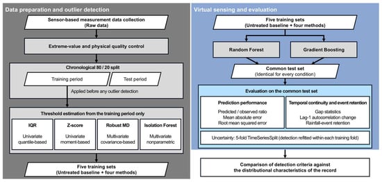
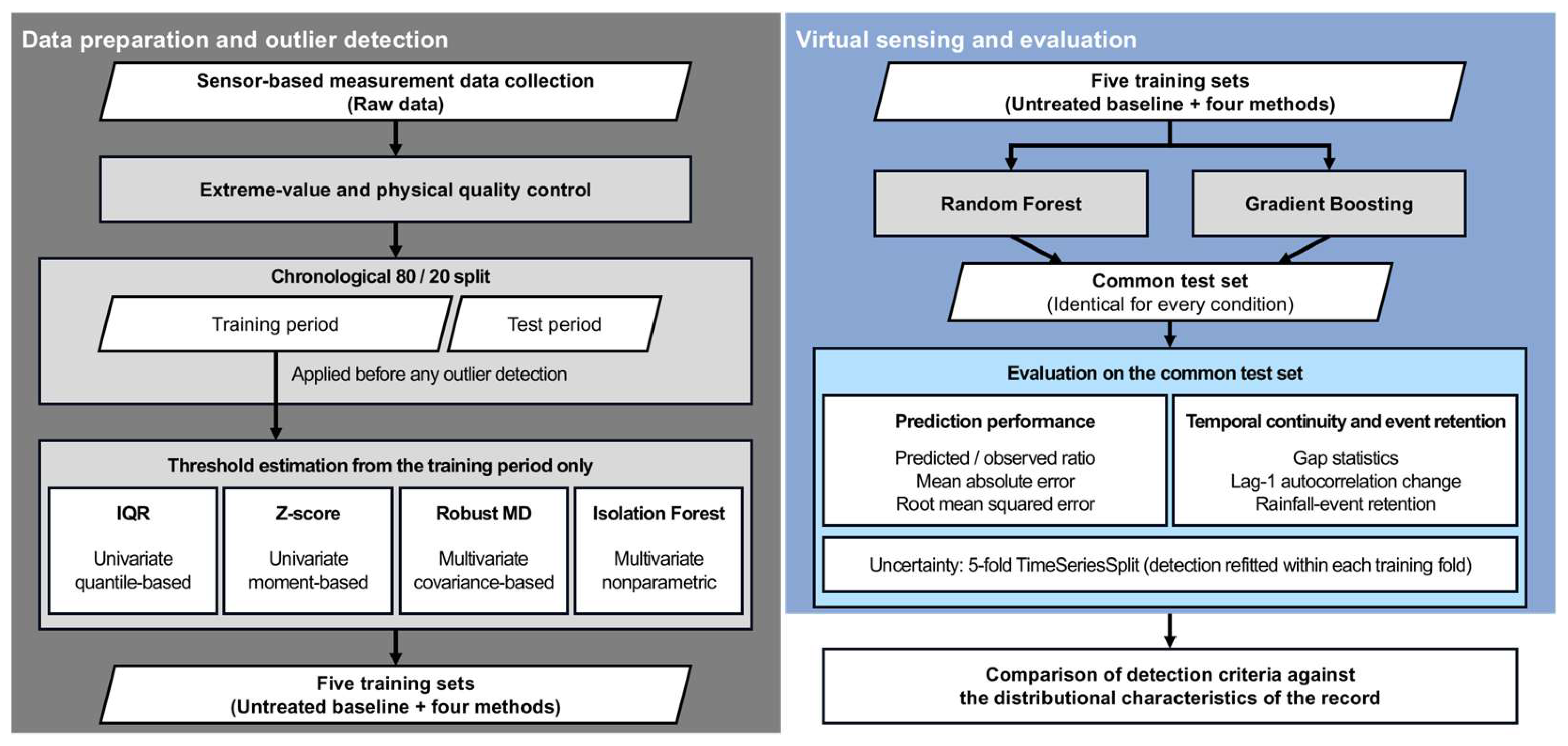
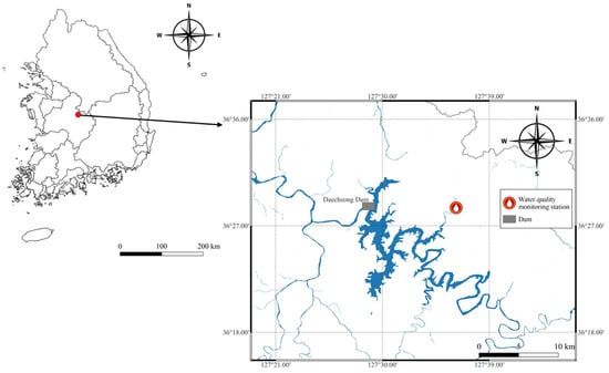
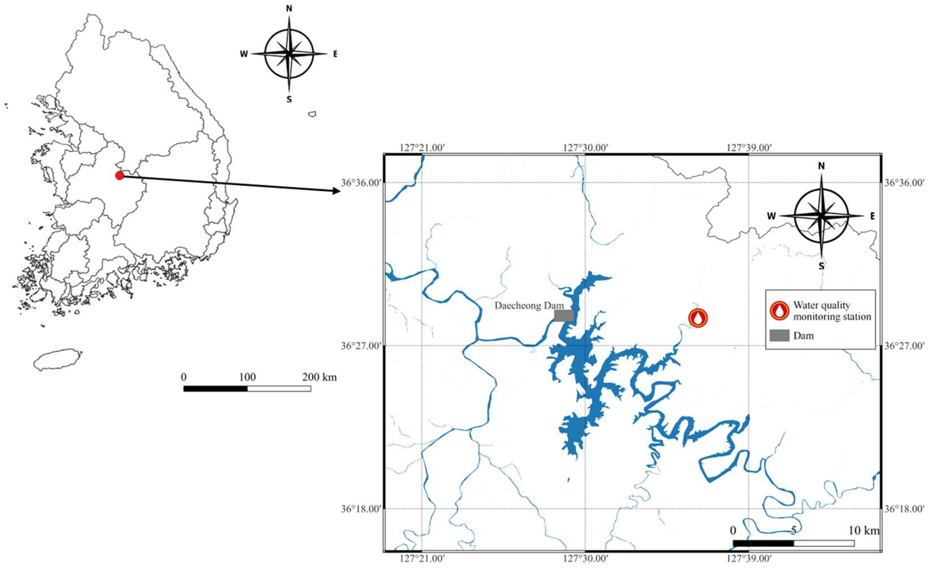
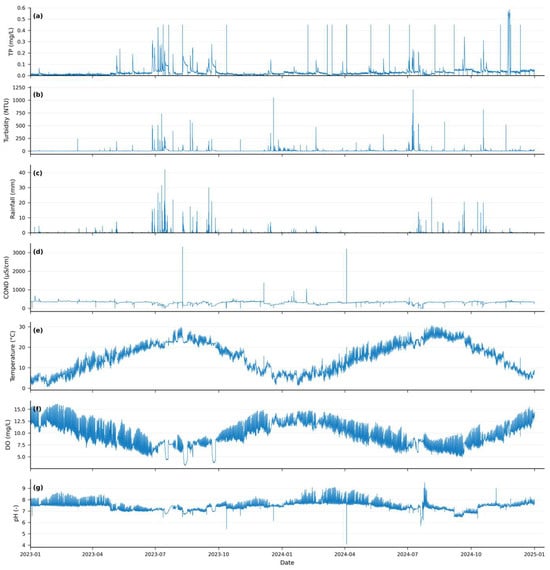
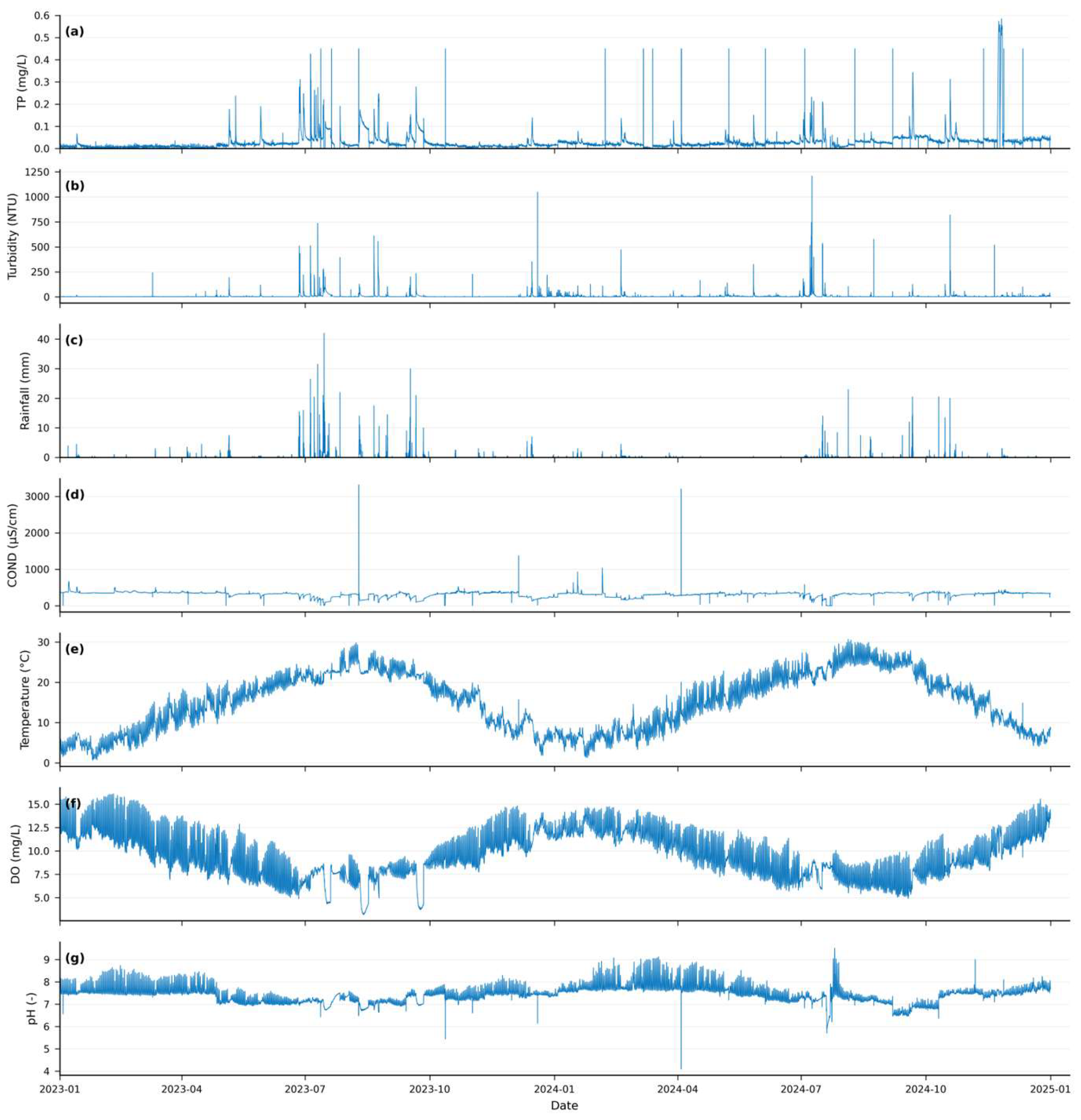
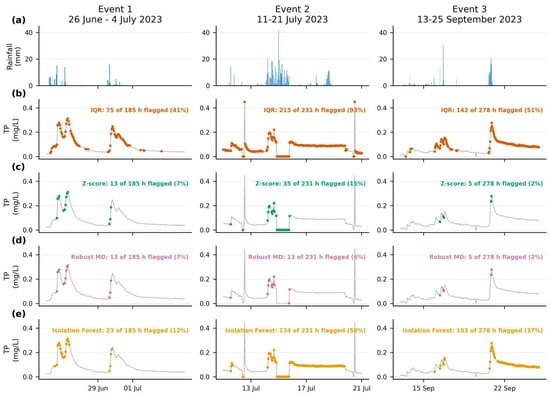
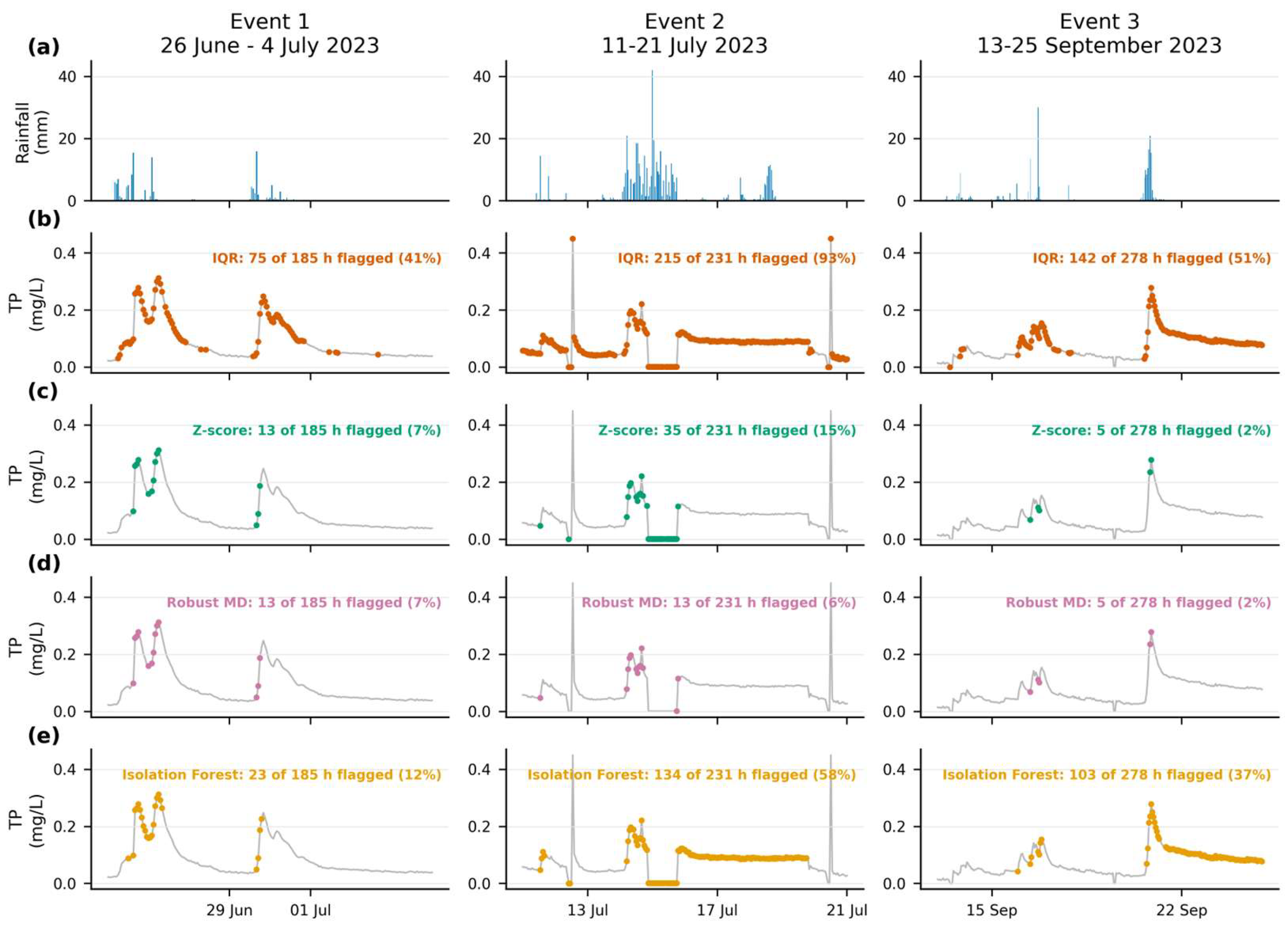
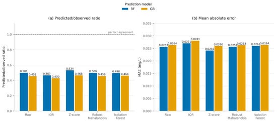
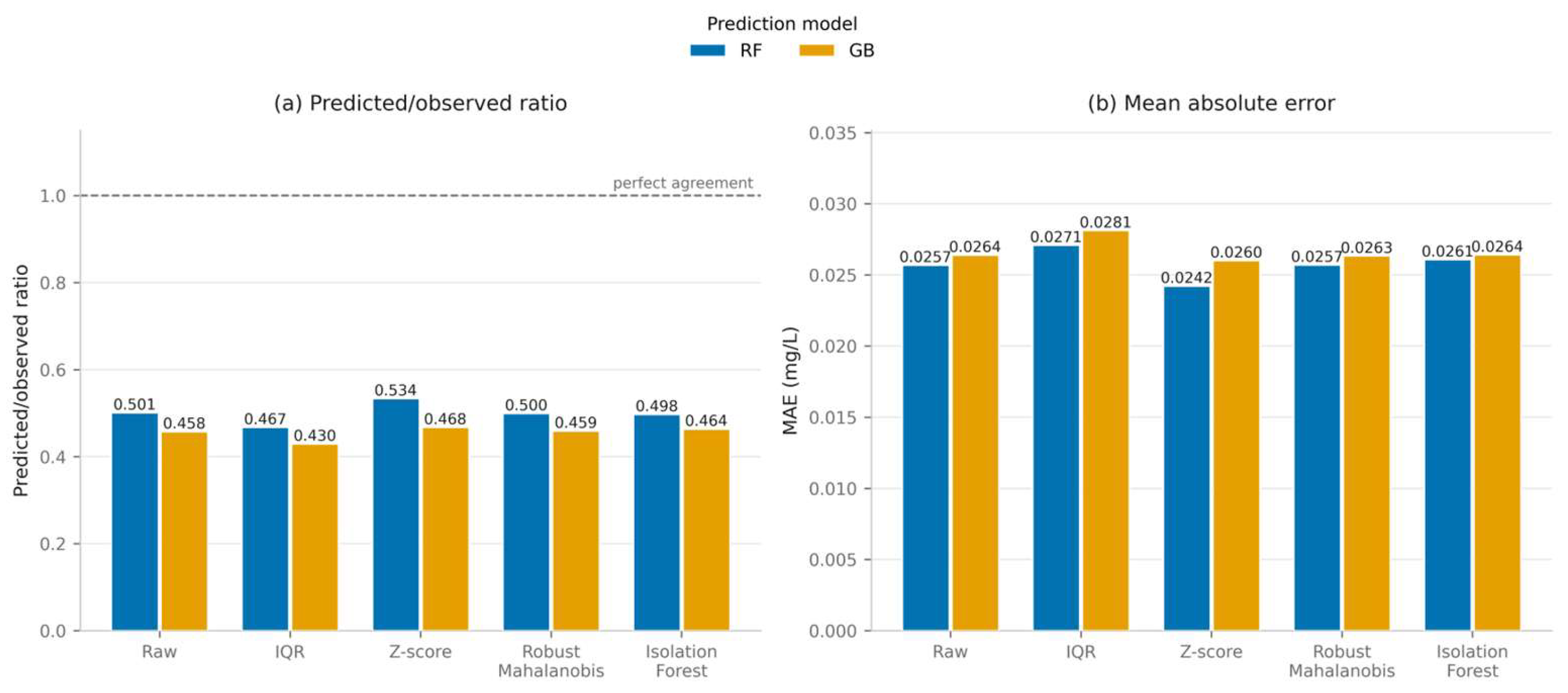

Disclaimer/Publisher’s Note: The statements, opinions and data contained in all publications are solely those of the individual author(s) and contributor(s) and not of MDPI and/or the editor(s). MDPI and/or the editor(s) disclaim responsibility for any injury to people or property resulting from any ideas, methods, instructions or products referred to in the content. |
© 2026 by the authors. Licensee MDPI, Basel, Switzerland. This article is an open access article distributed under the terms and conditions of the Creative Commons Attribution (CC BY) license.