Probabilistic Prediction and Reliability Analysis of Abutment Scour Depth Using Natural Gradient Boosting

Abstract

Reliable prediction of abutment scour requires accurate point estimates and quantification of predictive uncertainty. This study developed a NGBoost (Natural Gradient Boosting) framework using 297 laboratory observations under clear-water conditions across three abutment geometries. Hyperparameters were optimized using Optuna, with separate training, validation, calibration, and test sets. The model achieved a test-set R² of 0.980 and a root mean square error of 0.094. At the 95% nominal level, prediction-interval coverage was 96.67%, and the mean interval width was 26.69% smaller than that of split conformal prediction. Feature analyses identified the abutment Froude number and abutment geometry as important predictors. Monte Carlo simulation was used for a distribution-level reliability analysis based on independent sampling from measured and predictive scour-depth distributions. A design correction factor of 2.04 corresponded to a target reliability index of 1.5. The results demonstrate the potential of NGBoost for probabilistic abutment-scour assessment, while indicating the need for field validation and reliability analyses that account for dependence between measurements and predictions.

1. Introduction

Local scour around bridge abutments is a major cause of structural damage and collapse because it can undermine the stability of bridge foundations during floods [1]. Shirole and Holt reported that 823 bridges collapsed in the United States between 1950 and 1990 and that approximately 60% of these failures were associated with foundation scour [2]. Wardhana and Hadipriono analyzed 503 bridge failures that occurred in the United States between 1989 and 2000 and found that floods and scour accounted for the largest proportion, approximately 53% [3]. Scour-induced bridge damage can therefore have substantial socioeconomic consequences, including reconstruction costs, disruption of transportation networks, and loss of life [4].

Because the loss of foundation bearing capacity caused by scour has been identified as a major contributor to bridge failure, accurate prediction of scour depth has long been a central concern in bridge design and maintenance [5]. Abutment scour, however, arises from complex three-dimensional flow involving interactions among downflow, the horseshoe vortex, and the wake vortex, and consequently exhibits nonlinear behavior that depends on the flow conditions, bed conditions, and abutment geometry [1,6,7]. The complexity of these processes and the diversity of field conditions inevitably introduce predictive uncertainty. Safety-oriented design therefore requires a methodology that accounts for this uncertainty together with the predicted scour depth.

Efforts to predict scour depth have traditionally relied on empirical equations derived from experimental data. Representative equations for abutment scour include the Froehlich and HIRE equations presented in HEC-18; their simplicity and intuitive form have led to their widespread use in practice [5]. However, because these equations were developed under limited experimental conditions, they cannot readily accommodate diverse hydraulic conditions and abutment geometries simultaneously or fully represent the complex nonlinear relationships among the input variables [1,6,8]. Moreover, empirical equations differ in mathematical form and can yield substantially different estimates under identical conditions. Their basis in laboratory data can also limit their reliability under complex field conditions [9].

Numerical studies using computational fluid dynamics (CFD) have been actively pursued to address these limitations of empirical equations. Olsen and Kjellesvig used a three-dimensional numerical model based on the Reynolds-averaged Navier–Stokes equations and the k − ε turbulence model to calculate the maximum local scour depth around structures [10]. Comparisons with experimental results and empirical equations demonstrated the potential of CFD for scour prediction. Liu et al. combined the k − ε turbulence model with a sediment-transport model and an adaptive-grid technique to simulate scour development around a circular pier and a semicircular abutment [9]. Their model reproduced the scour geometry and maximum depth around the semicircular abutment in close agreement with the experiments, but produced comparatively large errors for pier scour because it did not adequately reproduce the horseshoe vortex upstream of the pier. Kumar and Afzal systematically investigated the effects of abutment geometry on local scour by combining numerical simulations with experiments [11]. Such numerical analyses provide valuable information on scour mechanisms by resolving the three-dimensional flow field and vortex structures around abutments. Nevertheless, their high computational cost and sensitivity to the selected turbulence and sediment-transport models limit their use in iterative design and routine engineering practice [12].

More recently, data-driven machine-learning (ML) methods have attracted attention as an alternative that can complement empirical equations and numerical analyses, and a range of algorithms have been applied to abutment-scour prediction. Khosravi et al. proposed hybrid models that combined KStar with several techniques and showed that models developed separately for each abutment geometry outperformed conventional empirical equations [13]. Kumar et al. developed a custom model that jointly learned from three abutment geometries (vertical-wall, semicircular, and 45° wing-wall abutments) and achieved high predictive accuracy under clear-water conditions [14]. Marulasiddappa et al. compared several ML models, including gradient tree boosting (GTB) and multivariate adaptive regression splines (MARS), for individual abutment geometries and reported particularly strong predictive performance of GTB for semicircular and 45° wing-wall abutments [15]. Collectively, these studies demonstrate that ML can learn complex nonlinear relationships and markedly improve scour-depth prediction. Most of them, however, evaluated performance using point-prediction performance metrics such as RMSE, MAE, and R² without explicitly quantifying predictive uncertainty.

Improved predictive accuracy alone is insufficient for engineering decision-making. In bridge design, both the mean prediction and its associated uncertainty must be considered to achieve an appropriate level of safety. For example, even if two models predict the same mean scour depth, the model with the wider predictive distribution indicates a greater possibility that the actual scour depth will substantially exceed the prediction and therefore calls for a more conservative design. Probabilistic prediction is thus needed to provide not only a point estimate but also an input-dependent predictive distribution.

This study aims to use natural gradient boosting (NGBoost) to estimate the conditional predictive distribution of abutment scour depth and to link predictive uncertainty to reliability-based design correction factors. Using the experimental data of Dey and Barbhuiya, an NGBoost model was developed in which the three abutment geometries were represented by a single categorical variable, and its hyperparameters were optimized using Optuna [8]. Point-prediction performance was benchmarked against conventional ML models, whereas probabilistic performance was compared with split conformal prediction and Gaussian process regression. The effects of the input variables were evaluated using SHAP, permutation importance, and ablation analysis. Finally, the predictive distribution was propagated through a Monte Carlo simulation to estimate design correction factors corresponding to target reliability levels.

2. Methods

2.1. Dimensional Analysis and Dataset

2.1.1. Dimensional Analysis

The equilibrium scour depth around an abutment d_s is governed by the flow conditions, bed material, and abutment geometry [1]. The principal influencing variables include the mean approach velocity U, flow depth h, abutment length L, median grain size d₅₀, gravitational acceleration g, water and sediment densities ρ and ρ_s, and abutment geometry. Applying the Buckingham π theorem expresses their relationship as the dimensionless function in Equation (1).

d_s/L = f(Fe, h/L, d₅₀/h, d₅₀/L, Type)

(1)

Among the dimensionless ratios in Equation (1), h/L, d₅₀/h, and d₅₀/L satisfy the relationship d₅₀/L = (d₅₀/h)(h/L) and are therefore algebraically dependent. Specifically, they exhibit the exact linear relationship log(d₅₀/L) = log(d₅₀/h) + log(h/L) in logarithmic space; consequently, including all three as inputs would violate the independence requirement of the dimensional analysis. These dimensionless variables (Fe, h/L, d₅₀/h, and d₅₀/L) have also been used in previous studies [13,14]. Whereas those studies used all four ratios, the present study excluded d₅₀/L to avoid the algebraic dependence described above and used the remaining three dimensionless variables (Fe, h/L, d₅₀/h) and the geometry variable Type as inputs, as shown in Equation (2). In contrast to previous approaches that either developed separate models for each abutment geometry or represented geometry as a continuous factor, the present study incorporated geometry as a categorical variable (Type) and trained a single model on all three geometries.

d_s/L = f(Fe, h/L, d₅₀/h, Type)

(2)

In Equation (1), Fe is the abutment Froude number defined by Equation (3), where s = ρ_s/ρ is the specific gravity of the sediment. Previous studies used the excess velocity U_e = U − ξU_c, where ξ is a geometry-specific coefficient and U_c is the critical velocity [8,13,14]. In the present study, however, the effect of geometry was represented explicitly by the categorical variable Type; therefore, Fe was calculated using the mean approach velocity U without applying a geometry-specific coefficient. This formulation allows Fe to represent flow intensity and Type to represent the effect of abutment geometry.

$$\mathit{Fe}=U/\sqrt{g\left(s-1\right)L}$$

(3)

2.1.2. Experimental Dataset

The analysis used clear-water equilibrium-scour experiments conducted by Dey and Barbhuiya [8]. The dataset comprises 297 experiments involving uniform sand (d₅₀ = 0.26–3.10 mm) and three abutment geometries: vertical-wall, semicircular, and 45° wing-wall abutments. Each geometry is represented by 99 experiments. The definitions and ranges of the input and target variables are summarized in Table 1.

Table 1. Definitions and ranges of the input and target variables (n = 297).

Variable	Definition	Min	Max
Fe	Abutment Froude number	0.16	0.83
h/L	Ratio of flow depth to abutment length	0.48	6.25
d50/h	Ratio of median grain size to flow depth	1.0 × 10−3	2.0 × 10−2
Type	Abutment geometry (0 = semicircular, 1 = 45° wing-wall, 2 = vertical wall)	0	2
ds/L	Dimensionless scour depth (target variable)	0.70	4.35

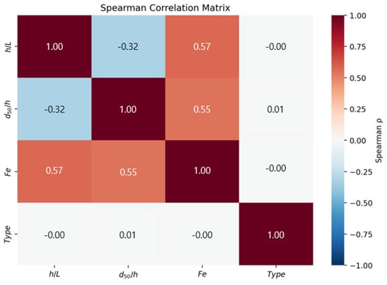
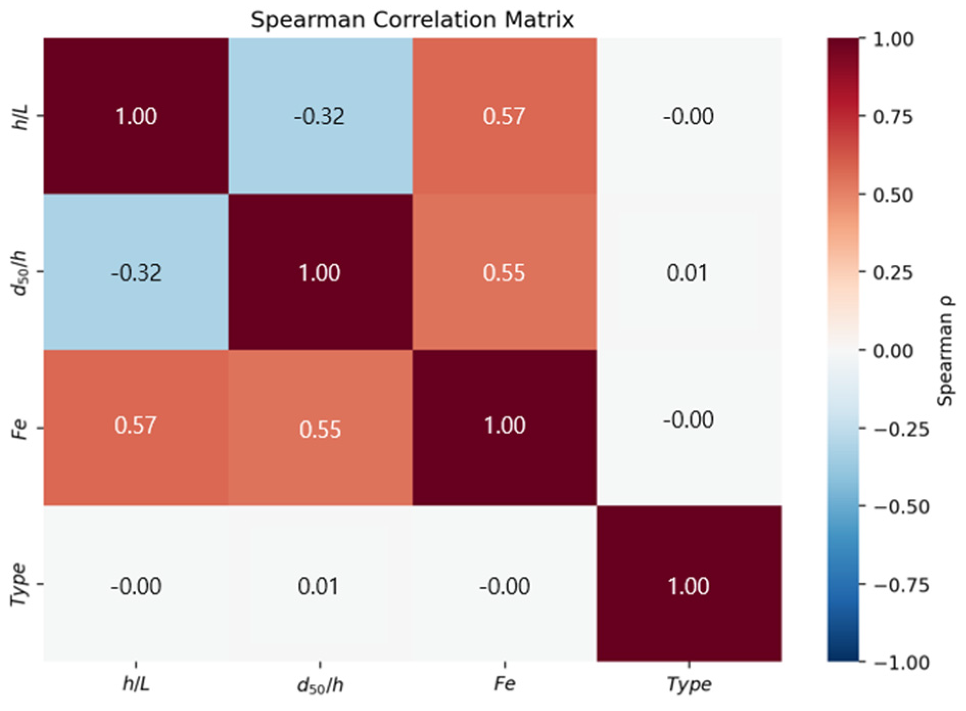
The correlation structure among the input variables was examined (Figure 1). The maximum Spearman correlation coefficient among the four inputs was 0.57, and neither exact algebraic dependence nor a very strong monotonic correlation was identified. Information redundancy among the inputs was therefore considered limited, supporting the interpretability of the subsequent feature-importance analysis.

Figure 1. Spearman rank correlation matrix among input variables.

2.1.3. Data Partitioning

Previous studies adopted a simple 70%/30% training-test split [13,14]. Although such a split can be adequate for evaluating point predictions, it provides no separate validation set for hyperparameter optimization. Repeatedly consulting test-set performance during hyperparameter selection effectively involves the test set in model selection. This practice introduces selection bias into performance estimation and may produce overly optimistic final results. To prevent such bias, the data used for hyperparameter selection must be separated from those used for performance evaluation [16].

The probabilistic predictions of NGBoost were also compared with split conformal prediction, which does not assume a specific parametric distribution such as the normal distribution [17,18,19]. Split conformal prediction constructs interval widths from prediction errors measured on a separate calibration set that was not used to train the model. If the calibration data used to determine interval width overlap with the test data used to evaluate coverage, performance is assessed on data that have already been used to tune the intervals and may consequently be inflated. The calibration and test sets must therefore remain separate [18].

To satisfy both requirements, the dataset was partitioned into training (70%, n = 207), validation (10%, n = 30), calibration (10%, n = 30), and test (10%, n = 30) sets. The validation set was used for Optuna-based hyperparameter optimization and early stopping, whereas the calibration set was used to construct the split conformal prediction intervals. More specifically, the calibration set was used to estimate empirical conformal quantiles and to conduct a preliminary assessment of the calibration of the NGBoost prediction intervals; the test set was reserved for final performance evaluation and post hoc sensitivity analyses. Separating the data used for model training, hyperparameter optimization, interval calibration, and final evaluation prevented the test set from influencing model fitting or hyperparameter selection. The random partitioning was performed with a fixed random seed. Because abutment geometry (Type) was included as an input, geometry information was incorporated directly into model training, and every subset contained all three geometries (approximately 27–37% per geometry).

To assess sensitivity to data partitioning, the dataset was randomly repartitioned ten times using different seeds while retaining the training/validation/calibration/test sample sizes of 207/30/30/30. The previously selected hyperparameters and model-training random seed were held fixed, and early stopping was performed using the validation set in each partition.

In addition, shuffled five-fold cross-validation was performed using all 297 observations with a random seed of 42. Each model was trained on four folds and evaluated on the remaining fold using the hyperparameters selected in the main experiment, without further hyperparameter optimization or validation-based early stopping. Performance was summarized using the mean and sample standard deviation across the five folds.

2.2. NGBoost-Based Probabilistic Prediction

2.2.1. NGBoost Model Configuration

Reliability-based design requires estimation of the conditional predictive distribution (p(y|x)) given the input conditions rather than a point estimate alone (y = f(x)). Accordingly, natural gradient boosting (NGBoost) was adopted [20]. NGBoost is a boosting model that uses decision trees as base learners and directly estimates the parameters of a conditional distribution, thereby returning a predictive distribution rather than only a point prediction.

NGBoost iteratively updates the parameters θ(x) of the conditional distribution P(y; θ(x)) to minimize a proper scoring rule. In this study, the conditional distribution was assumed to be normal, N(μ, σ²), and the logarithmic score was used as the scoring rule. The training objective, natural gradient, and parameter-update equation are given in Equations (4)–(6), respectively.

$$L\left(\theta \right)={\displaystyle \sum _{i=1}^n}S\left(y_i,{\theta }_i\right), S\left(y,\theta \right)=-\log p(y;\theta )$$

(4)

$$\tilde{\nabla }S\left(y,\theta \right)=I_s{\left(\theta \right)}^{-1}\nabla S(y,\theta )$$

(5)

θ_m(x) ← θ_m−1(x) − ηg_m(x)

(6)

In Equation (5), I_s(θ) denotes the Fisher information matrix. Because the natural gradient is invariant to parameterization, it provides more stable optimization than an ordinary gradient [21]. At boosting iteration m, the decision-tree base learners are fitted to the natural gradient, and the parameters are updated according to Equation (6). Here, g_m(x) denotes the fitted output multiplied by the iteration-specific scaling factor ρ_m obtained by line search, and η is the learning rate. A decision-tree regressor using the Friedman MSE criterion was employed as the base learner.

Residual normality was evaluated for the raw residuals in each data split using the Shapiro–Wilk test. Calibration of the predictive variance was additionally examined using the standard deviation of the standardized residuals Z = (y − μ)/σ. The corresponding results are presented in Section 3.3.

To assess sensitivity to the assumed normal output distribution, an additional NGBoost model with lognormal output was trained using the same hyperparameters, training random seed, and early-stopping rule. The models were compared using test-set NLL, CRPS, and 95% prediction-interval coverage and width. Sensitivity of α was evaluated using identical Copula-generated inputs and measured-distribution samples, with shared standard normal draws for predictive sampling. This comparison used a fixed model configuration rather than separate hyperparameter optimization for each output distribution.

2.2.2. Hyperparameter Optimization

The NGBoost model contains seven hyperparameters governing the boosting procedure and the base learner. To optimize all seven simultaneously, Optuna was used with the tree-structured Parzen estimator (TPE) algorithm [22,23]. The search comprised 150 trials.

Negative log-likelihood (NLL) on the validation set was used as the objective function. Because NLL evaluates both the predictive mean and predictive variance, it is suitable for assessing the fit of a conditional predictive distribution. The hyperparameter search spaces and optimal values are listed in Table 2. Among the 150 trials, the combination yielding the lowest validation NLL was selected; the resulting NLL was −0.892. This combination was retained for the full NGBoost model; the reduced models in the ablation analysis were separately reoptimized.

Table 2. Optuna-TPE hyperparameter search space and optimal values (150 trials).

Hyperparameter	Search Range	Search Type	Optimal
n_estimators	[50, 500]	integer uniform	362
learning_rate	[10−3, 0.3]	log-uniform	6.6 × 10−3
minibatch_frac	[0.5, 1.0]	uniform	0.53
col_sample	[0.5, 1.0]	uniform	0.55
max_depth	[2, 10]	integer uniform	8
min_samples_split	[2, 20]	integer uniform	2
min_samples_leaf	[1, 10]	integer uniform	3

2.3. Reliability-Based Estimation of Design Correction Factors

2.3.1. Construction of the Joint Input Distribution

To represent dependence among the Monte Carlo inputs, a Gaussian copula was constructed separately for each abutment geometry (Type). The full dataset of 297 observations was grouped by geometry. Within each group, the ranks of h/L, d₅₀/h, and Fe were converted to empirical cumulative probabilities and then to standard normal scores. The correlation matrix of these scores was used to parameterize the Gaussian copula. Geometry-specific empirical cumulative distributions were used as the marginal distributions. Type was sampled according to its observed frequency, with a probability of 1/3 for each geometry. Dependence reproduction was assessed by comparing the Spearman correlations of the observed data and the generated inputs, as summarized in Table 3.

Table 3. Comparison of Spearman correlations between observed data and Copula-generated inputs.

Variable Pair	Observed Data	Copula-Generated Inputs
h/L − Fe	0.5707	0.5930
d50/h − Fe	0.5467	0.5078
h/L − d50/h	−0.3178	−0.3037

2.3.2. Monte Carlo Propagation

The Type was first sampled according to the observed geometry frequencies. The three continuous inputs, h/L, d₅₀/h, and Fe, were then generated using the Gaussian copula and empirical marginal distributions corresponding to the sampled geometry. A total of 20,000 input samples were supplied to the trained NGBoost model, which returned the conditional predictive mean μ and standard deviation σ for each sample. A scour-depth sample S_i was drawn from each conditional normal distribution to form the aggregate predictive distribution, and negative predictive samples were set to zero. Separately, a lognormal distribution was fitted to the measured scour depths, and an equal number of samples R_i were drawn from this distribution independently of S_i.

2.3.3. Limit-State Function and Reliability Indices

The limit-state function incorporating the design correction factor α was defined by Equation (7). Here, R_i denotes a sample generated from the marginal distribution fitted to the measured scour depths, and S_i denotes a sample generated from the conditional predictive distribution returned by NGBoost for a Monte Carlo input condition. The two sets of Monte Carlo samples represent the overall characteristics of the measured scour-depth distribution and the NGBoost predictive distribution, respectively. In this study, they were sampled independently and compared at the distribution level.

g_i = R_i − αS_i

(7)

In Equation (7), the exceedance state g_i > 0 was defined as the case in which a sample from the measured distribution R_i exceeded the corrected prediction αS_i, where α is the correction factor. The scour-depth exceedance probability P_e, the Monte Carlo-based reliability index β_MC, and the Cornell reliability index β_normal were calculated using Equations (8)–(10), respectively.

P_e = P(g > 0) = E[1_{g>0}]

(8)

β_MC = −Φ⁻¹(P_e)

(9)

$${\beta }_{\mathit{normal}}=-{\displaystyle \frac{{\mu }_g}{{\sigma }_g}}$$

(10)

In Equation (10), the reliability index β_normal is defined as the negative ratio of the mean to the standard deviation of the limit-state function g [24]. Under the normal approximation for g, this sign convention ensures that β_normal increases as the defined scour-depth exceedance probability P(g > 0) decreases. The suitability of this approximation for the present data was examined by comparing β_MC with β_normal.

2.3.4. Back-Calculation of Design Correction Factors

The design correction factor α was varied from 0.5 to 4.0 in increments of 0.1, and Equations (7)–(10) were evaluated at each value. For each α, the scour-depth exceedance probability P_e, Monte Carlo-based reliability index β_MC, and Cornell reliability index β_normal were calculated to establish the α − β relationship. Linear interpolation was then performed at each target reliability index β to obtain the corresponding design correction factor α.

2.4. Model Evaluation

2.4.1. Performance Metrics

Point-prediction performance was evaluated using RMSE, MAE, and R². Probabilistic-prediction performance was evaluated in terms of calibration, sharpness, and overall distributional accuracy. These three aspects describe, respectively, how closely predicted probabilities agree with observed frequencies, how narrow the prediction intervals are, and how accurately the complete predictive distribution represents the observations.

Interval calibration was assessed using the prediction interval coverage probability (PICP), calculated using Equation (11). PICP is the proportion of observations contained within the prediction interval at a given nominal coverage level; values close to that level indicate well-calibrated intervals.

$$\mathrm{PICP}={\displaystyle \frac{1}{n}}{\displaystyle \sum _{i=1}^n}1\{L_i\le y_i\le U_i\}$$

(11)

Sharpness was evaluated using the mean prediction interval width (MPIW), calculated using Equation (12). MPIW is the average width of the prediction intervals, and a smaller value indicates a sharper interval provided that calibration is maintained.

$$\mathrm{MPIW}={\displaystyle \frac{1}{n}}{\displaystyle \sum _{i=1}^n}(U_i-L_i)$$

(12)

Overall distributional performance was evaluated using the continuous ranked probability score (CRPS) [25]. CRPS summarizes the agreement between the complete predictive distribution and the observation in a single score, thereby accounting for both predictive accuracy and uncertainty. For a normal predictive distribution N(μ, σ²), CRPS has the closed-form expression in Equation (13), and smaller values indicate closer agreement between the predictive distribution and the observed data.

$$\mathrm{CRPS}={\displaystyle \frac{1}{n}}{\displaystyle \sum _{i=1}^n}{\sigma }_i\left[z_i\left(2\mathsf{\Phi }\left(z_i\right)-1\right)+2\varphi \left(z_i\right)-{\displaystyle \frac{1}{\sqrt{\pi }}}\right], z_i={\displaystyle \frac{y_i-{\mu }_i}{{\sigma }_i}}$$

(13)

Here, μ_i and σ_i are the predictive mean and standard deviation for sample i, respectively, and Φ and ϕ are the cumulative distribution function and probability density function of the standard normal distribution, respectively.

2.4.2. Benchmark Models and Statistical Comparison

To benchmark the predictive performance of NGBoost, five comparison models (support vector regression, gradient boosting, random forest, extra trees, and a multilayer perceptron) were trained using the same data partition and Optuna-based hyperparameter optimization. Four simple baseline models were also evaluated to determine whether model performance exceeded the average structure of the data: k-nearest neighbors (k = 3), a single-hidden-layer extreme learning machine (h = 15), linear regression, and a mean predictor. All comparison and baseline models were finally fitted using the same 207 training observations as NGBoost. Where model selection was required, the separate validation set was used without incorporating its observations into the final fitting dataset.

Gaussian process regression (GPR) was additionally evaluated as an independent probabilistic baseline using the same 207 training observations as NGBoost. The continuous inputs were standardized, and Type was one-hot encoded, with preprocessing fitted only to the training data. RBF and Matérn kernels (ν = 1.5 and 2.5) were considered, each combined with a constant signal-amplitude kernel and a white-noise kernel. Kernel parameters were optimized using the training marginal likelihood, and the kernel family was selected using validation-set NLL without consulting the test set. The selected GPR model was compared with NGBoost using test-set RMSE, NLL, CRPS, PICP, and MPIW.

The statistical significance of differences in point-prediction performance was assessed using the Diebold–Mariano (DM) test [26]. This test determines whether the difference between the prediction errors of two models is statistically significant and therefore provides information not conveyed by error magnitudes alone. The loss differential $d_i=l\left(e_i^A\right)-l\left(e_i^B\right)$ was calculated, and the DM statistic was obtained by dividing the mean loss differential by its estimated standard error, as shown in Equation (14). The test was performed separately with squared error and absolute error as the loss function.

$$\mathrm{DM}={\displaystyle \frac{\overline{d}}{\sqrt{s_d^2/n}}}, \overline{d}={\displaystyle \frac{1}{n}}{\displaystyle \sum _{i=1}^n}{d}_i, s_d^2={\displaystyle \frac{1}{n-1}}{\displaystyle \sum _{i=1}^n}{(d_i-\overline{d})}^2$$

(14)

Split conformal prediction was applied to recalibrate the prediction intervals of the fitted NGBoost model [17,18,19]. The original and recalibrated intervals used the same NGBoost-predicted means and standard deviations, differing only in the interval coefficient. On the calibration set, nonconformity scores were calculated by dividing the absolute residuals by the predicted standard deviations, and an empirical quantile of these scores was used as the coefficient. Under exchangeability, split conformal prediction provides a distribution-free, finite-sample marginal coverage guarantee, which does not imply conditional coverage at every input condition or exact coverage in a particular test sample. The recalibrated test-set intervals were constructed using Equation (15). Here, δ denotes the nominal miscoverage rate, and ${\widehat{q}}_{\delta }$ is the finite-sample-adjusted empirical quantile of the calibration nonconformity scores for a target coverage of 1 − δ.

$${\mathit{PI}}_{\mathit{conf}}\left(x\right)=[\widehat{y}\left(x\right)-{\widehat{q}}_{\delta }\sigma (x), \widehat{y}\left(x\right)+{\widehat{q}}_{\delta }\sigma (x\left)\right]$$

(15)

2.4.3. Model Interpretability Analysis

Three methods, namely SHAP (SHapley Additive exPlanations), permutation importance, and ablation, were used to examine the contribution of each input variable from complementary perspectives. SHAP and permutation importance assess the contribution of a variable while retaining the remaining inputs, whereas ablation removes a variable and retrains the model, thereby also indicating whether the remaining variables can compensate for the omitted information. Comparing these perspectives distinguishes how each variable contributes to individual predictions from how essential it is to the model structure.

SHAP assigns a contribution to each variable for every prediction, and feature importance was evaluated using the mean absolute SHAP value [27]. Permutation importance was quantified as the increase in test-set mean squared error (MSE) after the values of a variable were randomly permuted, measuring its contribution to the performance of the fitted model [28]. For the ablation analysis, each input variable was removed in turn, and the model was initially retrained using the full-model hyperparameters. To assess the influence of hyperparameter mismatch after variable removal, each reduced model was additionally reoptimized using 150 Optuna trials over the same search space as the full model. Hyperparameters were selected by minimizing validation-set NLL, while the data partition and model-training random seed were held fixed. Test-set RMSE and R² were evaluated after model selection.

All analyses and visualizations were performed using Python 3.14.6 with NumPy 2.4.6, pandas 2.3.3, scikit-learn 1.9.0, NGBoost 0.5.11, Optuna 4.9.0, SHAP 0.52.0, SciPy 1.18.0, Matplotlib 3.11.0, and seaborn 0.13.2.

3. Results

3.1. Point-Prediction Performance and Generalizability

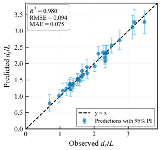
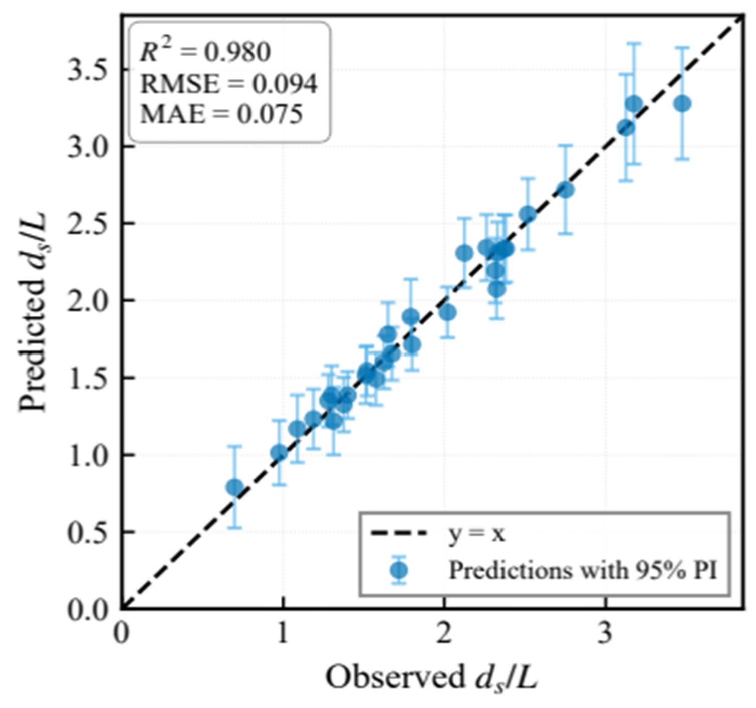
Table 4 summarizes the point-prediction performance of NGBoost across the four data splits. On the test set, NGBoost achieved R² = 0.980 and an RMSE of 0.094. In Figure 2, which compares predicted and measured values, most samples lie close to the 1:1 line, indicating close agreement between the predictions and measurements.

Table 4. Four-split point-prediction performance of NGBoost (n = 297, Optuna-tuned).

Split	n	RMSE	MAE	R2
Train	207	0.059	0.042	0.991
Validation	30	0.099	0.080	0.981
Calibration	30	0.155	0.095	0.951
Test	30	0.094	0.075	0.980

Figure 2. Comparison between NGBoost predictions and measured values for the test set.

In addition to point predictions, NGBoost provides a 95% prediction interval for each sample, distinguishing it from conventional deterministic models. The error bars in Figure 2 represent these intervals. Most measured values fall within the corresponding intervals, allowing point-prediction accuracy and predictive uncertainty to be assessed simultaneously. The resulting predictive distributions provide the basis for the subsequent evaluation of probabilistic performance and reliability.

The small difference in performance between the training and test sets (ΔR² = 0.011) provided no clear indication of overfitting for this particular data partition. Because generalizability cannot be established from a single partition, five-fold cross-validation was additionally performed to quantify variation in performance across data splits (Table 5).

Table 5. Fold-wise results of 5-fold cross-validation.

Fold	ntrain	ntest	RMSE	R2	NLL
1	237	60	0.118	0.968	−0.704
2	237	60	0.157	0.959	−0.802
3	238	59	0.114	0.965	−0.766
4	238	59	0.113	0.970	−0.753
5	238	59	0.093	0.971	−0.972
Mean	-	-	0.119	0.966	−0.799
Std.	-	-	0.023	0.005	0.103

Across the five folds, R² ranged from 0.959 to 0.971, with a mean of 0.966 ± 0.005. R² remained at or above 0.959 in every fold, indicating that overall predictive performance was consistently maintained across different data partitions. The difference in R² between the best and worst folds was approximately 0.012 and was attributed to variation in fold composition. Fold-wise NLL values ranged from −0.972 to −0.704, with a mean of −0.799, indicating that the performance of the conditional predictive distributions was also maintained across the folds. Across the ten repeated random partitions, the mean test-set RMSE and R² were 0.120 ± 0.018 and 0.962 ± 0.015, respectively, where ± denotes the sample standard deviation across partitions. The main experiment yielded a lower RMSE (0.094) and a higher R² (0.980) than these averages, suggesting that its data partition was relatively favorable.

3.2. Comparison with Benchmark Models and Statistical Significance Testing

NGBoost was compared with five machine-learning models using the same 207 training observations and the same test set. Test-set RMSE increased in the following order: gradient boosting (0.091), NGBoost (0.094), SVR (0.107), random forest (0.113), extra trees (0.120), and ANN (0.138) (Table 6). NGBoost therefore ranked second among the six machine-learning models. All four simple baselines produced larger RMSE values: ELM (0.131), linear regression (0.165), KNN (0.170), and the mean predictor (0.682).

Table 6. Test-set performance of NGBoost, comparison models, and baseline models using the same data split.

Model	RMSE	MAE	R2
Gradient Boosting	0.091	0.070	0.982
NGBoost	0.094	0.075	0.980
SVR	0.107	0.075	0.975
Random Forest	0.113	0.088	0.972
Extra Trees	0.120	0.096	0.968
ANN (MLP)	0.138	0.095	0.958
ELM (h = 15)	0.131	0.100	0.962
Linear Regression	0.165	0.138	0.940
KNN (k = 3)	0.170	0.125	0.936
Mean predictor	0.682	0.553	−0.027

NGBoost had a test-set RMSE approximately 3.5% higher than that of gradient boosting, the best-performing model in this comparison. The Diebold–Mariano test was applied to the sample-wise test losses to assess differences between NGBoost and the benchmark models (Table 7).

Table 7. Diebold–Mariano test results comparing NGBoost with each benchmark model using squared-error loss.

Comparison Model	DM Statistic	p-Value
Gradient Boosting	+0.180	0.857
SVR	−0.477	0.633
Random Forest	−1.450	0.147
Extra Trees	−2.093	0.036
ANN (MLP)	−1.496	0.135
ELM (h = 15)	−1.580	0.114
Linear Regression	−3.842	<10−3
KNN (k = 3)	−2.033	0.042
Mean predictor	−3.792	<10−3

At the nominal 5% significance level, using unadjusted two-sided p-values, NGBoost had significantly lower squared-error loss than extra trees (p = 0.036), KNN (p = 0.042), linear regression, and the mean predictor (both p < 10⁻³). Differences relative to gradient boosting, SVR, random forest, and ANN were not statistically significant. The difference relative to ELM was also nonsignificant (p = 0.114). The same significance pattern was obtained using absolute-error loss. However, the test set contained only 30 observations, limiting statistical power; nonsignificance does not establish equivalence, and the multiple pairwise comparisons should be interpreted as exploratory.

The RBF kernel was selected for GPR based on validation NLL. On the test set, GPR achieved lower RMSE, NLL, and CRPS than NGBoost and produced narrower prediction intervals (Table 8). However, its 95% intervals covered 26 of 30 observations, yielding a PICP of 86.67%, compared with 29 of 30 observations and a PICP of 96.67% for NGBoost. Thus, NGBoost provided higher realized coverage with wider intervals, whereas GPR performed better in point prediction and overall distributional scoring.

Table 8. Test-set point and probabilistic prediction performance of NGBoost and GPR.

Model	RMSE	NLL	CRPS	PICP at 95% (%)	MPIW at 95%
NGBoost	0.094	−0.939	0.053	96.67	0.435
GPR	0.075	−1.119	0.044	86.67	0.262

3.3. Probabilistic Prediction Quality and Calibration

This section evaluates the probabilistic predictions of NGBoost in terms of prediction-interval calibration, residual diagnostics, accuracy of the complete predictive distribution, and comparison with split conformal prediction.

Prediction-interval calibration was first evaluated using PICP. At nominal coverage levels of 50%, 80%, 90%, 95%, and 99%, test-set PICP values were 0.533, 0.933, 0.967, 0.967, and 1.000, respectively. The 80% interval was conservative, whereas the intervals at 90% and above were close to their nominal levels (Table 9). MPIW increased monotonically from 0.150 to 0.572 as the nominal coverage level increased. The slight overcoverage at the higher nominal levels indicates modestly conservative intervals.

Table 9. Test-set PICP and MPIW at five nominal coverage levels.

Nominal Level	PICP	PICP Deviation (pp)	MPIW
0.50	0.533	3.33	0.150
0.80	0.933	+13.33	0.285
0.90	0.967	+6.67	0.365
0.95	0.967	+1.67	0.435
0.99	1.000	+1.00	0.572

Residual normality differed among the data splits. The Shapiro–Wilk test did not reject normality of the raw residuals for the test and validation sets (test: W = 0.973, p = 0.620; validation: W = 0.985, p = 0.942), whereas normality was rejected for the training and calibration sets (training: W = 0.948, p < 0.001; calibration: W = 0.827, p < 0.001). The latter splits contained a small number of samples with relatively large prediction errors (see Section 3.6), resulting in skewed residual distributions. The standard deviation of the standardized residuals provides a direct diagnostic of the estimated predictive variance. For the calibration set, this value was 1.07, slightly above unity, suggesting a tendency to underestimate predictive variance; correspondingly, PICP was slightly below the nominal level for intervals of 80% and above. For the test set, the value was 0.87, below unity, suggesting a tendency to overestimate predictive variance. Test-set PICP exceeded the nominal level for all evaluated intervals, with the largest deviation at the 80% nominal level. The opposing patterns across the two splits indicate that the probabilistic calibration of NGBoost was generally satisfactory but varied somewhat with sample composition.

Accuracy was also evaluated over the complete predictive distribution rather than only through prediction intervals. The test-set CRPS, which summarizes agreement between the predictive distribution and the observation, was 0.053.

Table 10 compares the original NGBoost prediction intervals with conformal recalibrations of the same predictions. Both used the same predictive means and standard deviations; the original intervals used normal-theory coefficients, whereas the recalibrated intervals used empirical coefficients estimated from 30 calibration observations. At the 95% nominal level, the coefficients were 1.960 and 2.674, respectively. The original intervals covered 29 of 30 test observations (96.67%), whereas the recalibrated intervals covered all 30 (100.00%). The original intervals were approximately 26.69% narrower on this test set, but this width difference was accompanied by different realized coverage. With only 30 calibration observations, the empirical 95% coefficient is sensitive to the largest nonconformity scores. The observed width reduction therefore reflects this model and data partition and does not establish a general advantage over conformal recalibration. The NGBoost predictive distributions were retained for the subsequent Monte Carlo analysis.

Table 10. Comparison of prediction intervals from split conformal prediction and NGBoost.

Nominal	${\widehat{\mathit{q}}}_{\delta }$ (Conformal)	PICP (Conformal)	MPIW (Conformal)	z1−δ/2 (NGBoost)	PICP (NGBoost)	MPIW (NGBoost)	Width Reduction (%)
0.95	2.674	1.000	0.594	1.960	0.967	0.435	26.69
0.90	1.873	0.967	0.416	1.645	0.967	0.365	12.17
0.80	1.575	0.933	0.350	1.282	0.933	0.285	18.62

3.4. Feature Importance and Physical Mechanisms

Feature importance was examined using SHAP, permutation importance, and single-variable ablation (Table 11 and Table 12). The three methods quantify different aspects of importance. SHAP and permutation importance assess the contribution of a variable while the remaining variables are retained, whereas single-variable ablation removes a variable and retrains the model, thus indicating whether the remaining variables can compensate for the omitted information. Comparing these three perspectives distinguishes a variable’s contribution to individual predictions from its necessity within the model structure.

Table 11. SHAP and permutation importance (normalized to sum to 100%).

Variable	SHAP Normalized (%)	Permutation Importance (%)	SHAP Rank	Permutation Rank
Fe	38.9	59.6	1	1
Type	22.1	10.4	2	4
d50/h	21.5	18.7	3	2
h/L	17.4	11.3	4	3

Table 12. Single-variable ablation results with fixed and reoptimized hyperparameters.

Removed Variable	RMSE (Fixed)	RMSE (Reoptimized)	R2 (Reoptimized)
None (all 4)	0.094	-	-
h/L	0.158	0.130	0.963
d50/h	0.163	0.121	0.967
Fe	0.220	0.161	0.943
Type	0.230	0.226	0.887

SHAP and permutation importance produced partially different rankings. Both identified Fe as the most important variable, whereas Type ranked second in SHAP importance and last in permutation importance. SHAP measures the magnitude of contributions to individual predictions, while permutation importance measures the deterioration in fitted-model performance after a variable is shuffled. The lower permutation importance of Type may also partly reflect geometry-related information shared with other inputs, such as Fe and h/L. However, this possibility was not directly tested, and the observed rankings do not establish the extent of information redundancy among the variables.

Reoptimization reduced test-set RMSE for all reduced models (Table 12). After removing h/L, d₅₀/h, and Fe, the reoptimized RMSE values were 0.130, 0.121, and 0.161, respectively. Removing Type produced only a small improvement after reoptimization, from 0.230 to 0.226, and its RMSE remained 139.26% higher than that of the full model. Thus, Type removal continued to produce the largest performance loss after accounting for hyperparameter mismatch through reoptimization.

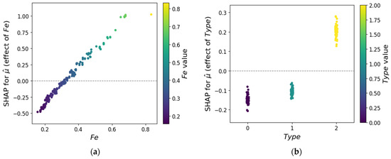
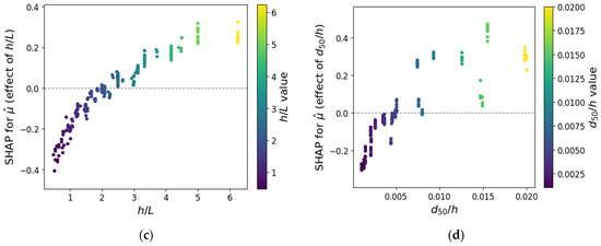
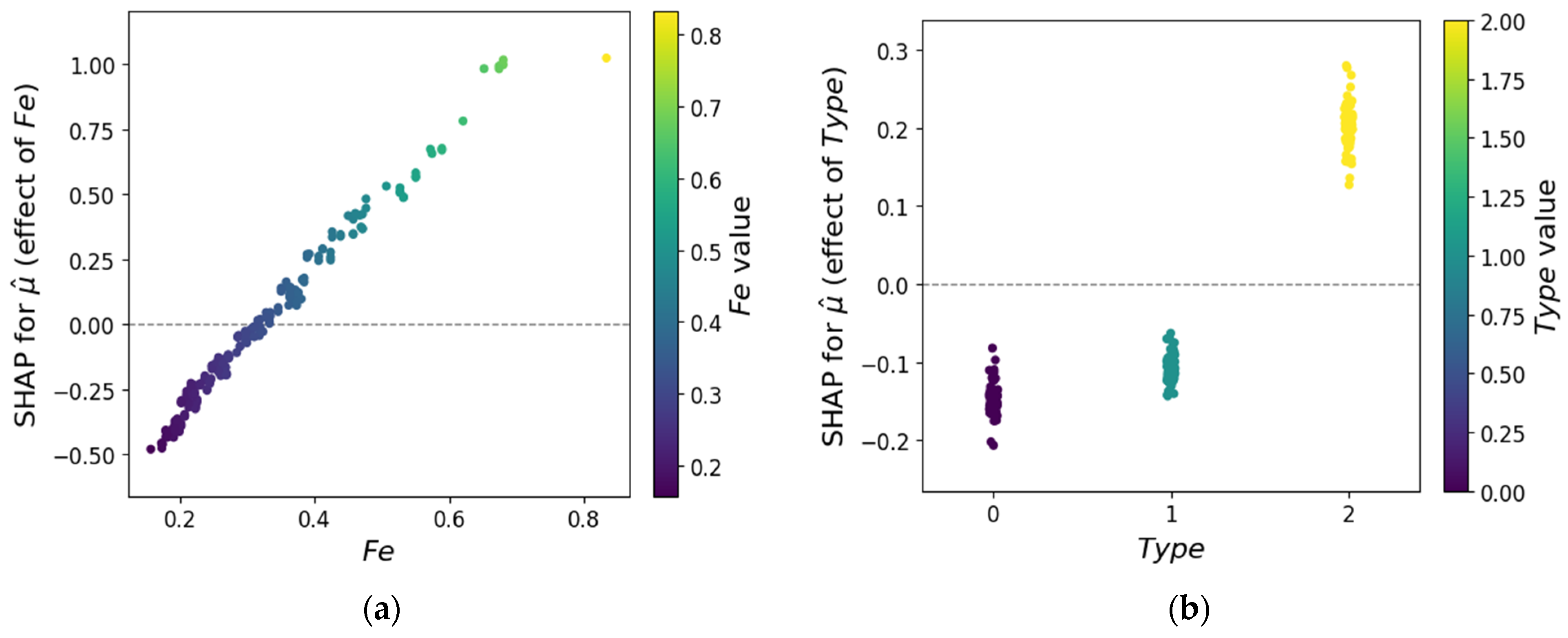
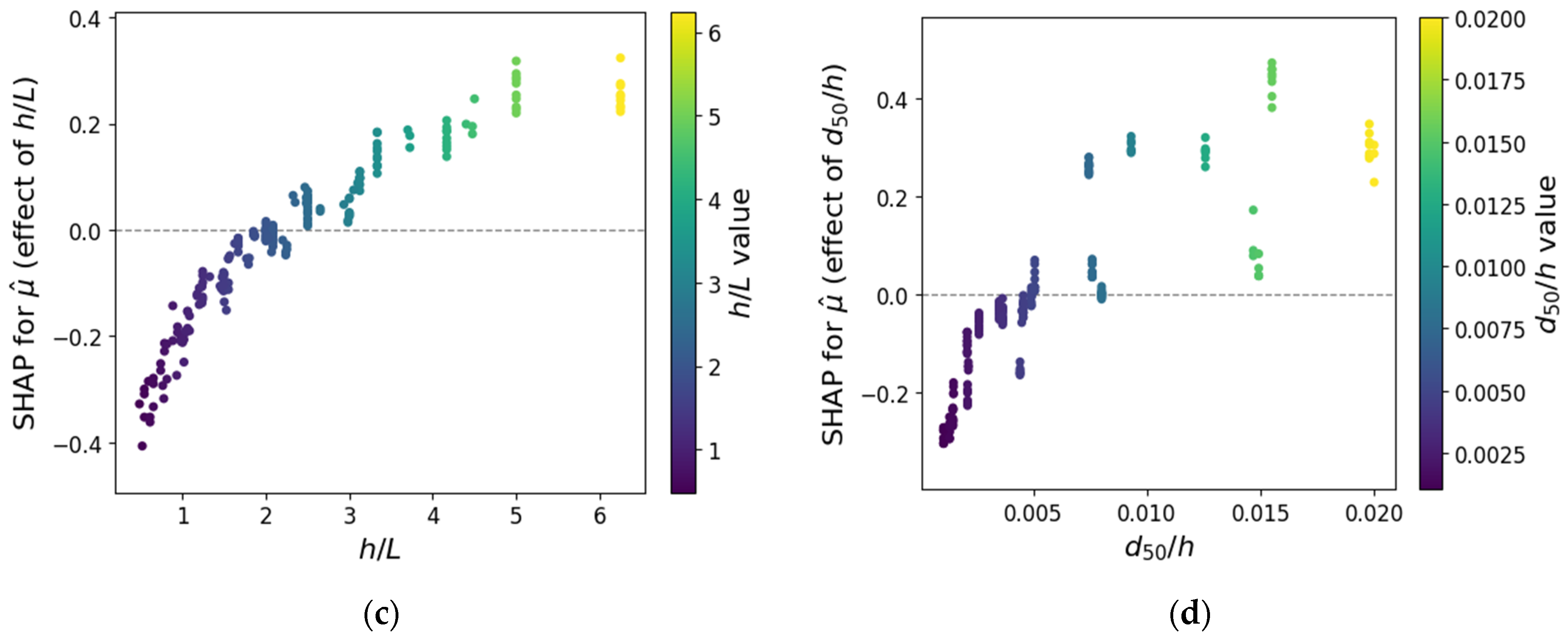
The relationships between the input variables and predictions were examined in detail using SHAP dependence plots (Figure 3). In the plot for Fe, the SHAP value increased markedly from −0.5 to +1.0 as Fe increased, confirming that Fe was the most influential continuous variable increasing predicted scour depth. In the plot for Type, SHAP values were clearly separated by abutment geometry (positive for vertical-wall abutments and negative for semicircular and 45° wing-wall abutments), demonstrating systematic geometry-dependent effects on the predictions. This pattern is consistent with both the largest performance loss caused by removing Type in the ablation analysis and the interpretation of Type as a regime variable. The plots for h/L and d₅₀/h showed generally increasing SHAP trends, although local variation was evident, particularly at the upper end of d₅₀/h. Their SHAP ranges were narrower than that of Fe, indicating smaller overall contributions.

Figure 3. SHAP dependence plots for each input variable: (a) Fe, (b) Type, (c) h/L and (d) d₅₀/h.

3.5. Derivation of Reliability-Based Design Correction Factors

The preceding sections established that the NGBoost predictive distributions were generally well calibrated. This section propagates those distributions through a Monte Carlo simulation to derive design correction factors corresponding to target reliability levels.

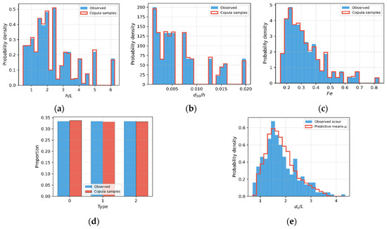
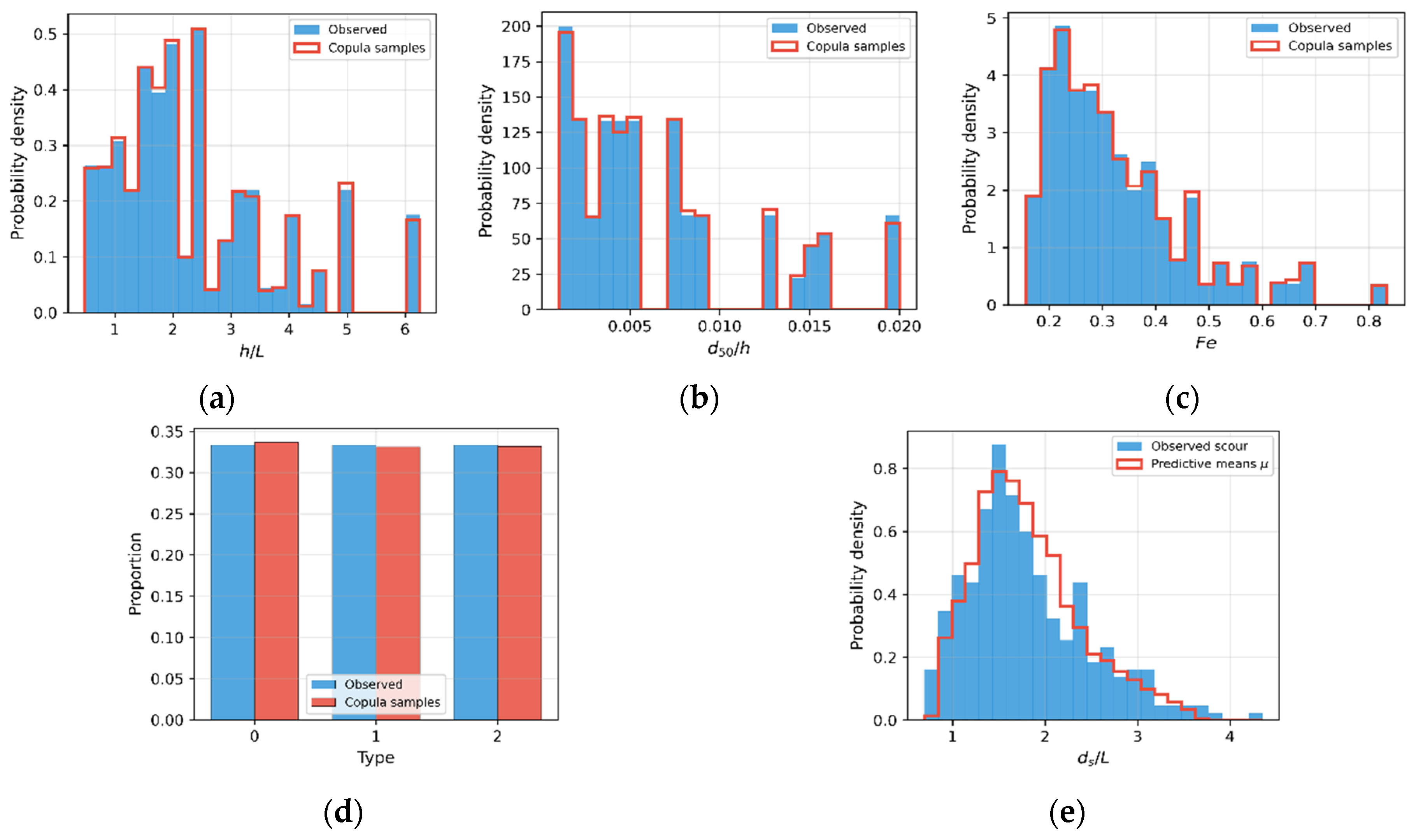
Figure 4a–d compare the marginal distributions of the observed data and the Copula-generated Monte Carlo inputs. The continuous inputs were generated using geometry-specific Gaussian copulas and empirical marginal distributions, while Type was sampled according to the observed geometry frequencies. The 20,000 generated scenarios broadly reproduced the observed marginal distributions and geometry proportions. As shown in Table 3, the generated Spearman correlations were 0.5930 for h/L–Fe, 0.5078 for d₅₀/h–Fe, and −0.3037 for h/L–d₅₀/h, approximately reproducing the observed dependence. Figure 4e compares the distribution of NGBoost predictive means μ across the generated scenarios with the measured scour-depth distribution.

Figure 4. Comparison of observed distributions and Copula-generated Monte Carlo distributions (n = 20,000): (a) h/L, (b) d₅₀/h, (c) Fe, (d) Type and (e) observed d_s/L and NGBoost predictive means μ_i.

For each generated scenario, the NGBoost model returned a predictive distribution, and the aggregate predictive statistics were obtained using the law of total variance. Under this law, the total predictive variance is the sum of the mean conditional predictive variance across scenarios, $E\left[{\sigma }_i^2\right]$, and the variance of the predictive means due to variation among input scenarios, Var(μ_i) [29]. The resulting overall predictive mean was 1.816, and the total predictive standard deviation, including the conditional predictive variance, was 0.582. These statistics characterize the conditional normal mixture before negative predictive samples were set to zero.

The aggregate predictive mean obtained using the Copula-generated inputs (1.816) was approximately 0.20% higher than the mean of the R_i samples drawn from the lognormal distribution fitted to the measured scour depths (1.813). The total predictive standard deviation (0.582) was approximately 86.60% of the standard deviation of the R_i samples (0.673). Thus, the two distributions had similar means, while the aggregate predictive distribution had a smaller spread as measured by standard deviation. This difference was considered when interpreting the exceedance probabilities and correction factors. Figure 4e shows the distribution of predictive means μ and should therefore be distinguished from the aggregate predictive distribution that also includes conditional predictive variance.

Using these input and predictive distributions, correction factors were derived for the target reliability levels following the procedures described in Section 2.3. Under the uncorrected condition (α = 1.0), the exceedance probability P(R > S) was 48.28%. This probability compares independently generated samples from the measured scour-depth distribution and the aggregate predictive distribution constructed using Copula-generated inputs. It should therefore be distinguished from the conditional probability of measured scour exceeding a prediction under identical input conditions.

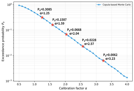
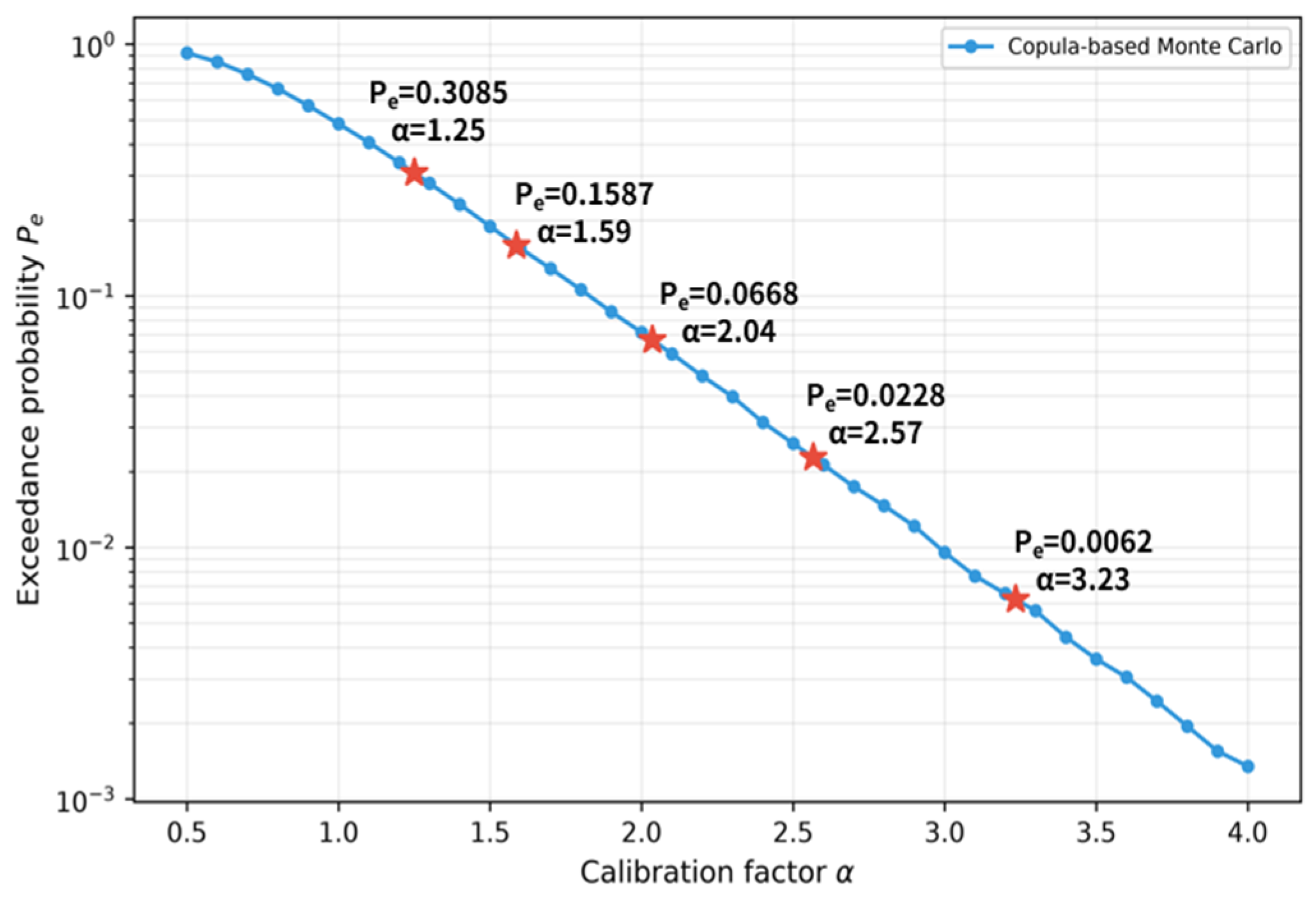
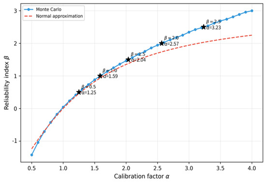
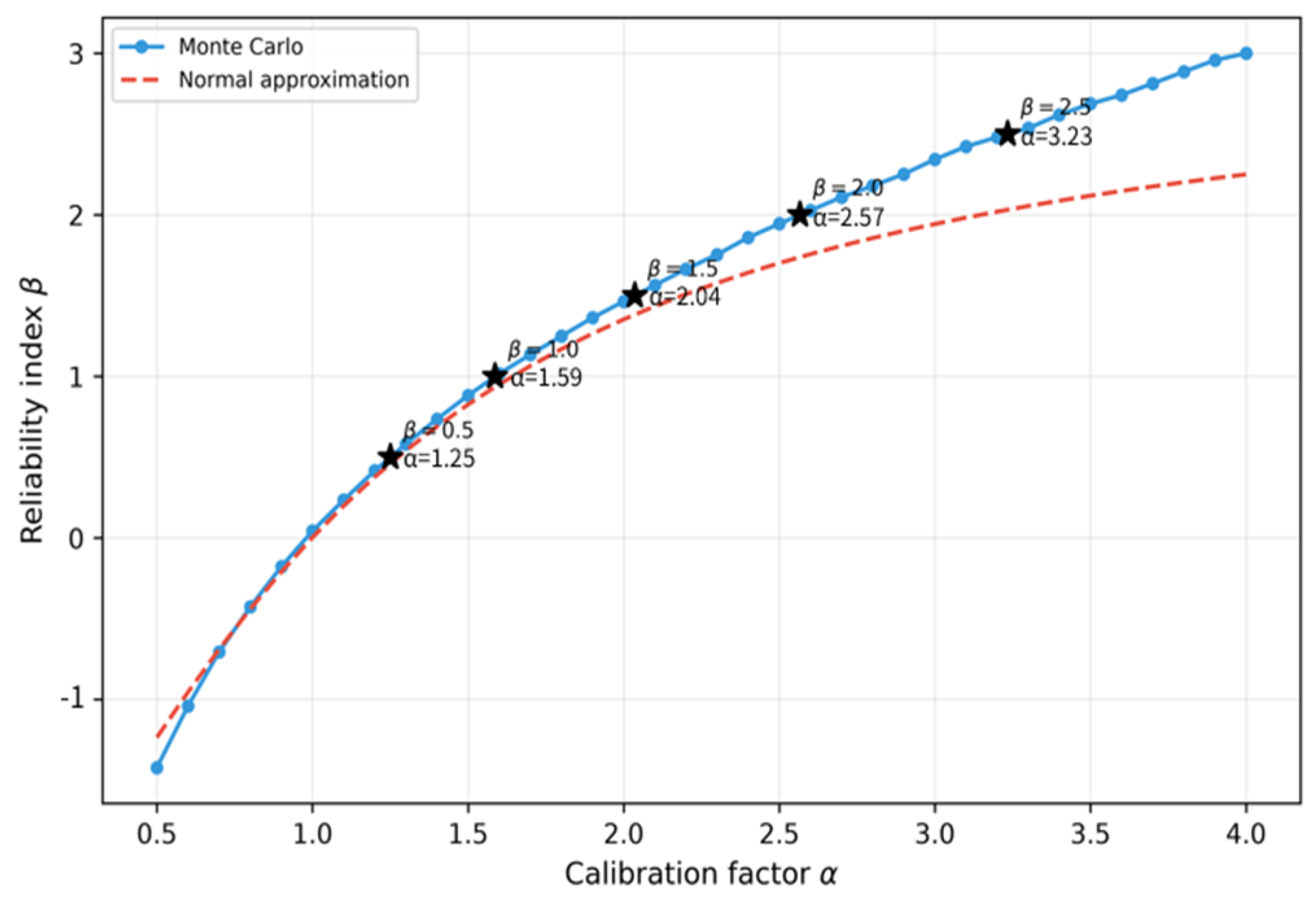
The correction factor α was varied from 0.5 to 4.0 in increments of 0.1. As α increased, the Monte Carlo-based reliability index increased monotonically, and the exceedance probability decreased monotonically (Figure 5 and Figure 6). The correction factors corresponding to target β values of 0.5, 1.0, 1.5, 2.0, and 2.5 were 1.25, 1.59, 2.04, 2.57, and 3.23, respectively.

Figure 5. Exceedance probability P_e = P(R_i > αS_i) as a function of the design correction factor α.

Figure 6. Reliability index β as a function of the design correction factor α.

Agreement between the normal approximation and direct Monte Carlo estimation was examined by comparing their reliability indices. Over the low correction-factor range of α = 0.50–1.20, the maximum absolute difference between the two reliability indices was 0.186 at α = 0.50, where the exceedance probabilities differed by 3.09 percentage points. At the interpolated target correction factors, the absolute differences were 0.040, 0.065, and 0.116 for target β values of 0.5, 1.0, and 1.5, respectively, but increased to 0.259 and 0.466 at target β values of 2.0 and 2.5. The normal approximation yielded lower reliability indices than direct Monte Carlo estimation at these target correction factors, with larger discrepancies at higher target β values. Correction factors were therefore determined using the directly estimated Monte Carlo exceedance probabilities.

3.6. Robustness Diagnostics

To determine whether the performance reported above was stable rather than restricted to a particular set of conditions, learning curves, observations with large prediction errors, uncertainty decomposition, and sensitivity to model configuration were examined.

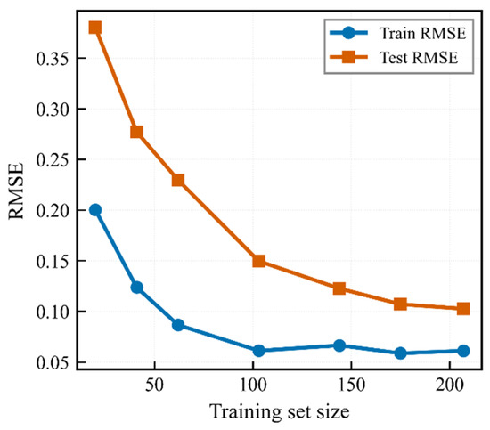
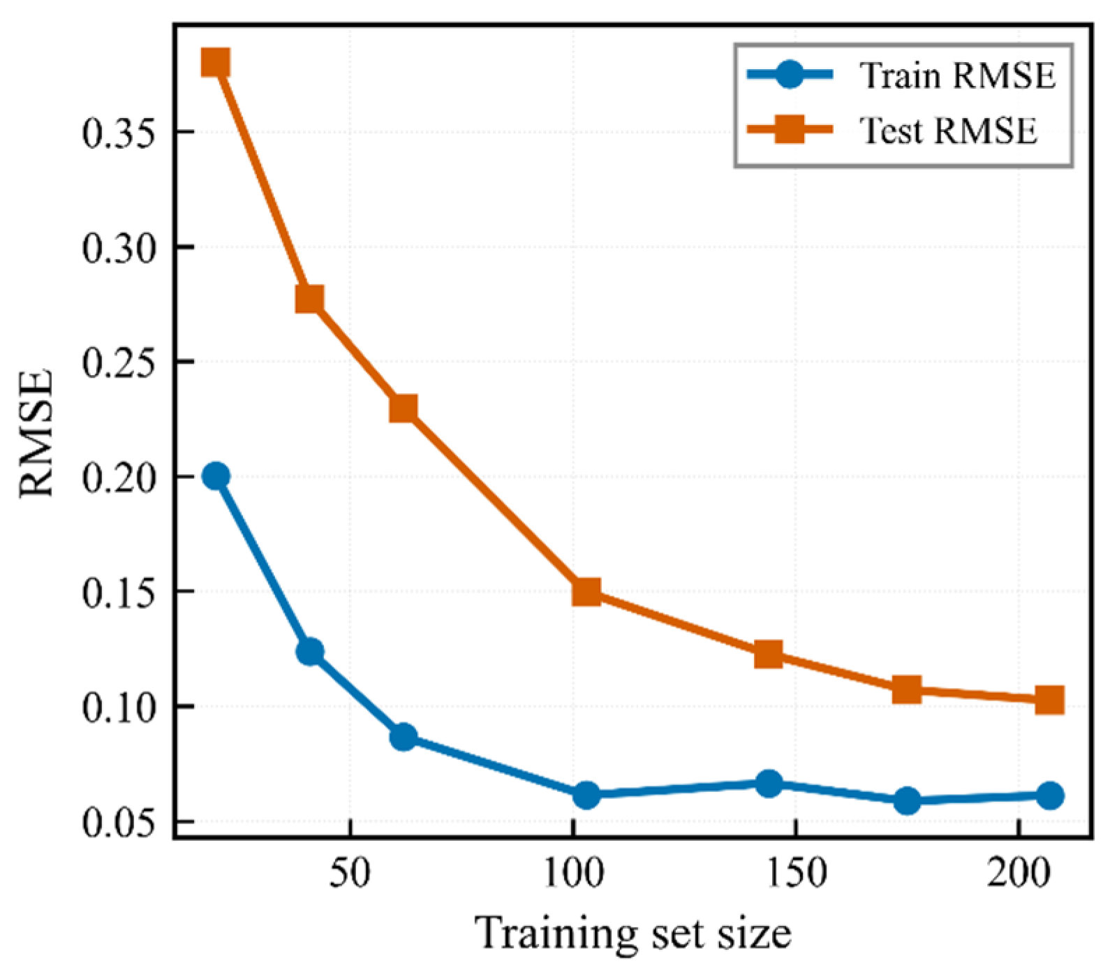
The learning-curve analysis showed that test-set RMSE decreased continuously as the training-set size increased (Figure 7). Test-set RMSE decreased from 0.380 at n_train = 20 to 0.150 at n_train = 103, 0.123 at n_train = 144, 0.107 at n_train = 175, and 0.103 at n_train = 207. The difference between the final two points was only 0.005, indicating that the curve had begun to plateau. Because a separate model was retrained at each dataset size, the RMSE at the final learning-curve point (0.103) differs slightly from the test RMSE of the final model (0.094). Overall predictive performance therefore appears to have largely stabilized at the current sample size. Nevertheless, additional observations in the sparsely sampled upper tail (d_s/L > 3) could improve predictive stability and uncertainty estimation under extreme-scour conditions.

Figure 7. Training and test RMSE as a function of training set size.

Examination of sample-wise prediction errors showed that sample 19 had the largest RMSE-normalized residual, 7.6, with a measured value of d_s/L = 4.35, a prediction of 3.72, and an absolute error of 0.626. Relatively large prediction errors were also observed for samples 118 (d_s/L = 3.78) and 237 (d_s/L = 3.08), both in the high-scour range. These samples were generally located at large values of Fe and d_s/L, within the sparsely populated upper tail of the dataset. They were therefore interpreted not as outliers that should be removed, but as diagnostics indicating that predictive stability may be limited under extreme-scour conditions.

Predictive uncertainty was decomposed using a bootstrap analysis (B = 100). The mean estimated epistemic, aleatoric, and combined standard deviations across the test samples were 0.067, 0.107, and 0.127, respectively. Based on the mean component variances across the test samples, epistemic uncertainty accounted for approximately 29.09% of the total predictive variance, whereas aleatoric uncertainty, represented by the conditional predictive distribution of NGBoost, accounted for approximately 70.91%. Epistemic uncertainty can be reduced by adding data, whereas aleatoric uncertainty reflects the inherent variability of the data. Additional observations would therefore be expected to reduce the epistemic component primarily.

Sensitivity to model-configuration choices was also examined. Integer and one-hot encoding of the Type variable produced test-set RMSE values of 0.094 and 0.099, respectively, a difference of only 0.005; thus, the post hoc sensitivity analysis indicated little difference in performance between the two encoding schemes. A nine-variable model formed by adding nonlinear transformations and interaction terms to the four original inputs produced a slightly higher test-set RMSE of 0.096, indicating no performance gain from the derived variables. This result suggests that NGBoost can learn the required nonlinear relationships from the original inputs alone and that additional derived variables, which could reduce interpretability, are unnecessary for the present model.

4. Discussion

On the test set, NGBoost achieved R² = 0.980 and an RMSE of 0.094, a level of point-prediction accuracy numerically comparable to that reported in previous studies using the same dataset from Dey and Barbhuiya [8]. The custom model of Kumar et al., trained jointly on all abutment geometries, achieved R² = 0.96 and an RMSE of 0.132, so the RMSE obtained here is 28% lower, and Khosravi et al., who trained separate models for each geometry, reported an RMSE of 0.084 for their WIHW-KStar model on vertical-wall abutments-a range the present model approached despite being trained jointly on all three geometries [13,14]. These comparisons indicate that a single model incorporating abutment geometry as a categorical variable can attain point-prediction performance comparable to that of geometry-specific models. NGBoost ranked second in test-set RMSE among the six machine-learning models after their final training-set sizes were matched at 207 observations. The DM test did not detect a significant loss difference relative to gradient boosting, the only higher-ranked model, whereas NGBoost had lower loss than extra trees at the nominal 5% level. The independent GPR comparison showed that performance depended on the evaluation criterion: GPR achieved lower RMSE, NLL, and CRPS, whereas NGBoost provided 95% prediction-interval coverage closer to the nominal level, although with wider intervals. This closer agreement with the nominal coverage, together with competitive point-prediction accuracy, supported retaining NGBoost for the subsequent uncertainty propagation and reliability analysis. However, this advantage was observed on a test set of only 30 observations and does not establish overall superiority to GPR.

Beyond point accuracy, the probabilistic predictions were generally well calibrated. Prediction intervals at the 90% nominal level and above were close to their nominal coverage, and the slight overcoverage at higher levels indicates modestly conservative intervals. In scour prediction, where underestimation can pose a direct risk to structural safety, such conservatism may be preferable from a design perspective. Comparison with conformal recalibration showed that the original NGBoost intervals were approximately 26.69% narrower at the 95% nominal level, with realized test coverage of 96.67% compared with 100.00% for the recalibrated intervals. Because both intervals used the same NGBoost predictions, this comparison evaluates alternative interval coefficients rather than independent probabilistic models. The width difference depends on the calibration sample, particularly the largest nonconformity scores among the 30 observations, and should therefore be interpreted as a result specific to this data partition. The test-set CRPS of 0.053 provides an additional measure of predictive distributional accuracy, but these results alone do not establish calibration in the extreme tails required for reliability assessment.

The differing raw-residual normality results across data splits motivated a quantitative sensitivity assessment of the output-distribution assumption. Because predictive standard deviations vary with the inputs, pooled raw residuals need not follow a single normal distribution even under a conditionally normal model. To assess the practical impact of the distributional choice, normal and lognormal NGBoost models were compared using the same hyperparameters, training random seed, and early-stopping rule. The models yielded test-set NLL values of −0.9394 and −0.9393 and CRPS values of 0.0529 and 0.0542, respectively. Both 95% prediction intervals covered 29 of the 30 test observations, giving identical coverage of 96.67%. Mean interval widths were 0.4354 and 0.4636, respectively, making the lognormal intervals approximately 6.5% wider.

Under identical Copula-generated inputs, changing the output distribution from normal to lognormal increased α at target β = 1.5 from 2.04 to 2.06, a relative change of approximately 1.03%. Across target β values of 0.5–2.5, relative changes in α ranged from −0.69% to +1.48%. Within this fixed-configuration comparison, the normal model provided the same realized 95% test coverage with narrower intervals, while the estimated correction factors showed limited sensitivity to the distributional change. These results support retaining the normal output distribution for the primary analysis.

The feature-importance results also lend themselves to a physical interpretation. The different roles of Type and Fe in scour prediction can be understood through the underlying flow mechanisms. Abutment geometry alters the vortex structures generated as the flow passes around the abutment [1]: vertical-wall abutments generate strong horseshoe vortices and downflow, producing greater scour, whereas the smoother redirection of flow around semicircular and 45° wing-wall abutments reduces vortex intensity and scour depth. Consequently, the baseline scour depth differs among abutment geometries even at the same Fe, and when Type is removed, a single function must describe observations generated under distinct vortex regimes, causing the prediction error to increase sharply. Type can thus be interpreted as a regime variable that distinguishes the mechanism under which scour develops, whereas Fe is an intensity variable that describes changes in scour depth with flow intensity within a given regime. This interpretation is consistent with Khosravi et al., who reported consistently high Pearson correlations of 0.957–0.978 between Fe and scour depth when models were trained separately for each geometry, and it also supports the ability of joint training with explicit geometry information to approach the performance of geometry-specific models [13].

The Copula-based reliability analysis showed that higher target β values required progressively larger increases in α. Raising the target β from 0.5 to 1.0 increased α from 1.25 to 1.59, whereas raising β from 2.0 to 2.5 increased α from 2.57 to 3.23. Thus, larger increases in the correction factor were needed to achieve the same increment in β at higher target levels. The estimated factor α = 2.04 at target β = 1.5 should be interpreted within hydraulic and geological conditions identical or similar to those represented in the training data. Specifically, the dataset covers clear-water equilibrium scour in uniform noncohesive sediment and three regular abutment geometries. Outside these conditions, the factor may underestimate the required correction if actual scour is greater relative to predictions, or overestimate it if predictions are more conservative. Without external validation, however, neither the direction nor the magnitude of this potential bias can be quantified. The discrepancy between the normal approximation and direct Monte Carlo estimation increased at higher target β values. Direct Monte Carlo estimates were therefore used to determine α in the present analysis.

Several limitations should nevertheless be borne in mind. First, the sample size (n = 297) is relatively small for a machine-learning study; although the learning curve had largely plateaued, the data remained sparse in the upper tail, and additional observations are needed to improve predictive stability under extreme-scour conditions, with domain-adaptation methods likely required if field and laboratory data are later combined. Second, because the analysis relied on a single laboratory dataset, further validation is required for field environments beyond the clear-water, uniform-sand, noncohesive conditions considered here, including mixed soils, debris effects, nonuniform flow, and cohesive sediments. External validation using an independent dataset was not performed in this study, and deviations in α across datasets remain to be evaluated. Third, raw-residual normality was rejected for the training and calibration sets, and relatively large errors occurred in the upper tail. Although a fixed-configuration lognormal comparison showed unchanged 95% test coverage and small changes in α, Student-t output and separate hyperparameter optimization for each distribution were not evaluated. The small test sample also limits conclusions about tail coverage. Further assessment of alternative output distributions is therefore needed. Fourth, input dependence was represented using geometry-specific Gaussian copulas and empirical marginal distributions. However, the selected copula structure may not reproduce all aspects of dependence, and empirical marginals do not support extrapolation beyond the observed range. Sensitivity to alternative copula structures and marginal representations therefore warrants further investigation. Fifth, the reliability analysis independently sampled the marginal distribution of measured scour depth and the NGBoost predictive distribution, so the resulting exceedance probabilities and correction factors represent a distribution-level comparison rather than a conditional reliability analysis under identical input conditions; extending the framework to a conditional analysis that accounts for the dependence between actual scour and its prediction at the same inputs is an important direction for future research. These limitations define the scope within which the present results should be interpreted and identify priorities for future work.

5. Conclusions

This study used NGBoost to estimate the conditional predictive distribution of abutment scour depth and linked it to a Monte Carlo-based reliability analysis to derive reliability-based design correction factors. The principal findings are as follows.

First, NGBoost achieved a test-set R² of 0.980 and an RMSE of 0.094, ranking second among the six machine-learning models fitted using 207 training observations. The DM test detected no significant loss difference relative to gradient boosting. At the nominal 5% level, NGBoost had lower loss than extra trees, KNN, linear regression, and the mean predictor. Given the limited test sample and unadjusted pairwise tests, these findings are exploratory and do not establish equivalent performance where differences were nonsignificant.

Second, the probabilistic predictions from NGBoost were generally well calibrated on the test set. At the 95% nominal level, the original NGBoost intervals were narrower than the conformally recalibrated intervals, with PICP values of 0.967 and 1.000, respectively. The test-set CRPS, which measures agreement between the complete predictive distribution and the observations, was 0.053. Compared with GPR, NGBoost achieved higher realized 95% coverage with wider intervals, whereas GPR yielded lower CRPS, demonstrating different strengths across the evaluated metrics.

Third, the feature-importance analysis identified Fe as an intensity variable describing continuous changes in scour depth and Type as a regime variable distinguishing the mechanisms under which scour develops. Taken together, the SHAP, permutation-importance, and single-variable ablation results indicated that these variables play complementary roles, consistent with the physical mechanisms of abutment scour.

Fourth, the distribution-level reliability analysis used Copula-generated inputs and independently sampled measured and predictive scour-depth distributions. The exceedance probability under the uncorrected condition was 48.28%, and the illustrative correction factors corresponding to target β values of 1.5 and 2.5 were 2.04 and 3.23, respectively. Differences between the normal approximation and Monte Carlo-based reliability indices increased at higher target β values; correction factors were determined using direct Monte Carlo estimates.

This study extends abutment-scour assessment from point estimates to predictive distributions and establishes a framework for determining correction factors corresponding to target distribution-level exceedance probabilities. By explicitly quantifying the relationship between predictive uncertainty and correction levels, the framework provides a quantitative basis for the future development of reliability-based scour-design methods. The estimated correction factors are illustrative results specific to the dataset and distribution-level comparison adopted in this study, rather than generally applicable design recommendations. Engineering application requires external validation using independent field scour data representative of the intended application conditions, together with reliability assessment based on comparisons under identical input conditions.

References

- Melville, B.W.; Coleman, S.E. Bridge Scour; Water Resources Publications: Highlands Ranch, CO, USA, 2000. [Google Scholar]
- Shirole, A.M.; Holt, R.C. Planning for a comprehensive bridge safety assurance program. Transp. Res. Rec. 1991, 1290, 39–50. [Google Scholar]
- Wardhana, K.; Hadipriono, F.C. Analysis of recent bridge failures in the United States. J. Perform. Constr. Facil. 2003, 17, 144–150. [Google Scholar] [CrossRef] [Scilit]
- Brandimarte, L.; Paron, P.; Di Baldassarre, G. Bridge pier scour: A review of processes, measurements and estimates. Environ. Eng. Manag. J. 2012, 11, 975–989. [Google Scholar] [CrossRef] [Scilit]
- Arneson, L.A.; Zevenbergen, L.W.; Lagasse, P.F.; Clopper, P.E. Evaluating Scour at Bridges, 5th ed.; Hydraulic Engineering Circular No. 18 (HEC-18), FHWA-HIF-12-003; Federal Highway Administration: Washington, DC, USA, 2012.
- Ettema, R.; Yoon, B.; Nakato, T.; Muste, M. A review of scour conditions and scour-estimation difficulties for bridge abutments. KSCE J. Civ. Eng. 2004, 8, 643–650. [Google Scholar] [CrossRef] [Scilit]
- Dey, S.; Raikar, R.V. Characteristics of horseshoe vortex in developing scour holes at piers. J. Hydraul. Eng. 2007, 133, 399–413. [Google Scholar] [CrossRef] [Scilit]
- Dey, S.; Barbhuiya, A.K. Time variation of scour at abutments. J. Hydraul. Eng. 2005, 131, 11–23. [Google Scholar] [CrossRef] [Scilit]
- Liu, S.; Yang, Y.; Wu, X. Simulations of local scour around a cylindrical bridge pier and a semicircular abutment using unsteady k–ε model combined with σ-grid. Open Civ. Eng. J. 2017, 11, 598–614. [Google Scholar] [CrossRef] [Scilit][Green Version]
- Olsen, N.R.B.; Kjellesvig, H.M. Three-dimensional numerical flow modeling for estimation of maximum local scour depth. J. Hydraul. Res. 1998, 36, 579–590. [Google Scholar] [CrossRef] [Scilit]
- Kumar, L.; Afzal, M.S. Computational fluid dynamics modeling of scour around abutment geometries under combined effects of waves and currents. Ocean Eng. 2024, 294, 116812. [Google Scholar] [CrossRef] [Scilit]
- Huang, W.; Yang, Q.; Xiao, H. CFD modeling of scale effects on turbulence flow and scour around bridge piers. Comput. Fluids 2009, 38, 1050–1058. [Google Scholar] [CrossRef] [Scilit]
- Khosravi, K.; Khozani, Z.S.; Mao, L. A comparison between advanced hybrid machine learning algorithms and empirical equations applied to abutment scour depth prediction. J. Hydrol. 2021, 596, 126100. [Google Scholar] [CrossRef] [Scilit]
- Kumar, L.; Afzal, M.S.; Ghosh, S. A novel-tuned custom ensemble machine learning model to predict abutment scour depth in clear water conditions. AQUA Water Infrastruct. Ecosyst. Soc. 2023, 72, 798–813. [Google Scholar] [CrossRef] [Scilit]
- Marulasiddappa, S.B.; Patil, A.P.; Kuntoji, G.; Praveen, K.M.; Naganna, S.R. Prediction of scour depth around bridge abutments using ensemble machine learning models. Neural Comput. Appl. 2024, 36, 1369–1380. [Google Scholar] [CrossRef] [Scilit]
- Cawley, G.C.; Talbot, N.L.C. On over-fitting in model selection and subsequent selection bias in performance evaluation. J. Mach. Learn. Res. 2010, 11, 2079–2107. [Google Scholar]
- Vovk, V.; Gammerman, A.; Shafer, G. Algorithmic Learning in a Random World; Springer: New York, NY, USA, 2005. [Google Scholar] [CrossRef] [Scilit]
- Lei, J.; G’Sell, M.; Rinaldo, A.; Tibshirani, R.J.; Wasserman, L. Distribution-free predictive inference for regression. J. Am. Stat. Assoc. 2018, 113, 1094–1111. [Google Scholar] [CrossRef] [Scilit]
- Angelopoulos, A.N.; Bates, S. Conformal prediction: A gentle introduction. Found. Trends Mach. Learn. 2023, 16, 494–591. [Google Scholar] [CrossRef] [Scilit]
- Duan, T.; Anand, A.; Ding, D.Y.; Thai, K.K.; Basu, S.; Ng, A.; Schuler, A. NGBoost: Natural gradient boosting for probabilistic prediction. In Proceedings of the 37th International Conference on Machine Learning (ICML), Virtual, 13–18 July 2020; PMLR: Cambridge, MA, USA, 2020; Volume 119, pp. 2690–2700. [Google Scholar]
- Amari, S. Natural gradient works efficiently in learning. Neural Comput. 1998, 10, 251–276. [Google Scholar] [CrossRef] [Scilit]
- Bergstra, J.S.; Bardenet, R.; Bengio, Y.; Kégl, B. Algorithms for hyper-parameter optimization. Adv. Neural Inf. Process. Syst. 2011, 24, 2546–2554. [Google Scholar]
- Akiba, T.; Sano, S.; Yanase, T.; Ohta, T.; Koyama, M. Optuna: A next-generation hyperparameter optimization framework. In Proceedings of the 25th ACM SIGKDD International Conference on Knowledge Discovery & Data Mining, Anchorage, AK, USA, 4–8 August 2019; ACM: New York, NY, USA, 2019; pp. 2623–2631. [Google Scholar] [CrossRef] [Scilit]
- Cornell, C.A. A probability-based structural code. ACI J. 1969, 66, 974–985. [Google Scholar] [CrossRef] [Scilit] [PubMed]
- Gneiting, T.; Raftery, A.E. Strictly proper scoring rules, prediction, and estimation. J. Am. Stat. Assoc. 2007, 102, 359–378. [Google Scholar] [CrossRef] [Scilit]
- Diebold, F.X.; Mariano, R.S. Comparing predictive accuracy. J. Bus. Econ. Stat. 1995, 13, 253–263. [Google Scholar] [CrossRef] [Scilit]
- Lundberg, S.M.; Lee, S.-I. A unified approach to interpreting model predictions. Adv. Neural Inf. Process. Syst. 2017, 30, 4765–4774. [Google Scholar]
- Breiman, L. Random forests. Mach. Learn. 2001, 45, 5–32. [Google Scholar] [CrossRef] [Scilit]
- Der Kiureghian, A.; Ditlevsen, O. Aleatory or epistemic? Does it matter? Struct. Saf. 2009, 31, 105–112. [Google Scholar] [CrossRef] [Scilit]
Disclaimer/Publisher’s Note: The statements, opinions and data contained in all publications are solely those of the individual author(s) and contributor(s) and not of MDPI and/or the editor(s). MDPI and/or the editor(s) disclaim responsibility for any injury to people or property resulting from any ideas, methods, instructions or products referred to in the content. |
© 2026 by the authors. Licensee MDPI, Basel, Switzerland. This article is an open access article distributed under the terms and conditions of the Creative Commons Attribution (CC BY) license.