Coastline Evolution of Large-Scale Artificial Beach Nourishment in the Vicinity of a Newly Built Breakwater: An Empirical Case Study from the South Baltic Coast

Abstract

Large-scale beach nourishment projects constructed adjacent to port breakwaters may produce spatially contrasting shoreline responses because wave transformation, sediment redistribution, and structural effects act simultaneously. This study presents an empirical analysis of short-term shoreline evolution at a large artificially nourished beach constructed next to the eastern breakwater of the Vistula Spit Channel in the South Baltic Sea. The analysis combines historical orthophotomaps, monthly Real-Time Kinematic Global Positioning System (RTK-GPS) shoreline surveys, drone-based elevation data, hourly wave records, and tide-gauge observations collected between February 2024 and March 2025. The objective was to quantify the spatial and temporal variability of shoreline change and to interpret the observed erosion and accretion in relation to wave conditions, sea-level variability, the presence of the breakwater, and post-nourishment sediment redistribution. Historical shoreline changes were assessed at fixed coastal mileage locations. Monthly shoreline changes were quantified using a polygon-based on Geographic Information System (GIS) procedure, with gross erosion, gross accretion, and net area change calculated for successive survey intervals. Two characteristic 250 m coastal sectors were also compared: the area adjacent to the breakwater and the eastern boundary of the monitored beach. Approximately 55,550 m² of erosion and 57,851 m² of accretion were identified during the monitoring period, resulting in a net positive balance of approximately 2301 m². The small net value masks substantially larger opposing changes in different parts of the study area. The sector adjacent to the breakwater showed a predominantly negative cumulative surface balance, whereas the eastern sector showed a predominantly positive balance. The May–June interval was not uniformly stable, despite generally moderate offshore wave conditions, because a net loss of approximately 9626 m² was recorded. The results indicate that shoreline evolution was controlled by the combined effects of offshore wave forcing, sea-level variability, wave transformation near the breakwater, initial nourishment geometry, and natural post-nourishment sediment redistribution. Offshore wave parameters were not treated as direct nearshore forcing because refraction, shoaling, diffraction, breaking, and energy dissipation may modify the wave field before it reaches the shoreline. The study provides an empirical description of short-term shoreline adjustment rather than a validated predictive model.

1. Introduction

The coastline is the outline of the average water-level position along the cross-shore profile. The position of this line is subject to continuous changes caused either by fluctuations in the water level of the sea (gravity and infragravity waves, tides, and storm surges), erosion or accumulation of the shore, or both factors simultaneously. The description of coastline variability depends on the adopted spatio-temporal scales and the simplifications applied. Spatial scales can range from hundreds of meters to many tens of kilometers, and temporal scales range from a few hours to many years. The scale of simplifications pertains to the method of applying mathematical description. On the one hand, there are approaches based on classical mechanics, which rely on the principles of conservation of mass, momentum, and energy; on the other hand, there are methods for assessing coastline variability based on long-term telemetric observations. The latter allow for the subjective identification of characteristic points of the coastline, and the obtained results are static, local, or at most regional in nature, as they do not stem from general functional relationships describing coastal variability but rather from a specific series of aerial photographs taken for a given coastal area and their interpretation. Examples of such approaches include the works of Short [1] with many subsequent modifications, Wright [2], Sunamura [3], Rudowski [4], and Furmańczyk [5].

From a physics perspective, the spatio-temporal evolution of the coastline is most often predicted using the theories and models of one or multiple lines, as presented by Kraus [6] and Larson and Kraus [7]. The underlying philosophy generally assumes that the topography of the coastal zone can be described by single lines representing key isobaths. The simplest description of coastline variability is provided by the one-line model. In this model, the characteristic line is the intersection of the mean sea level with cross-shore profiles (the zero isobath), and all other isolines are parallel to it. An additional assumption is that cross-shore profiles along the coast are constant and uniform in shape. Consequently, coastline variability in this description is equivalent to the onshore or offshore movement of the cross-shore profile while maintaining its shape.

Multi-line models are generally based on the same principles as the one-line model, with the key difference being that they incorporate n-characteristic lines (isobaths of the coastal zone) (Reeve and Fleming [8]). Besides the coastline, these may include other significant elements of the cross-shore profile, such as bars, longshore accretion-erosion deposits, or other seabed features that abruptly alter the profile’s morphology or character. Each such line represents a part of the profile (a region of the coastal zone) that may change independently of other areas. While one-line models typically account only for longshore sediment transport, multi-line theories also consider onshore and offshore sediment transport. The most common multi-line theories are two- or three-line models.

Process-based numerical modeling has undergone substantial advancements in recent decades, enabling the simulation of coastal morphological processes, the quantification of sediment transport rates, and the evaluation of bathymetric evolution across multiple temporal scales (Dastgheib [9]; Guo [10]; and Huang [11]). These models integrate the principal hydrodynamic drivers acting upon the seabed, including tidal currents, wave action, wave-induced circulation, and sediment fluxes. To address these complexities, a suite of specialized software packages such as Delft3D, XBeach, TELEMAC-2D, DHI Mike 21, and CMS has been developed, offering enhanced flexibility and computational capacity for coastal system analysis.

Traditionally, long-term simulations of coastal morphodynamics, extending over months to years, were computationally intensive and time-consuming. The introduction of the Morphological Acceleration Factor (MAF) scheme (Benedet et al. [12]; Karathanasi & Belibassakis [13]) has markedly improved computational efficiency. In this approach, wave climate data are first reduced to a set of representative conditions that serve as hydrodynamic boundary inputs. Subsequently, the bathymetric changes computed at each hydrodynamic time step are scaled by the MAF, and the adjusted bathymetry is applied in the ensuing hydrodynamic calculations.

The MAF methodology rests on the critical assumption that morphological responses to hydrodynamic forcing remain linear within each morphological time step. While this assumption facilitates accelerated computations, it may introduce systematic errors and biases, particularly in coastal environments characterized by highly variable wind and wave regimes (Knappen & Joustra [14]; Malliouri et al., [15]). Moreover, the optimal range of MAF values is region-specific and lacks universal applicability (Ranasinghe et al. [16]). Therefore, model outputs should be rigorously validated against observed bathymetric changes, with particular emphasis on sites exhibiting dynamic morphological behavior, to ensure reliability and accuracy.

These different research approaches have been used worldwide in numerical modeling of hydrodynamics, lithodynamics, and morphodynamics. In coastal zones, nonlinear, quasi-random processes of coastal mechanics are further characterized by a certain inertia in the shoreline’s response to hydrodynamic forces and are still incompletely understood; therefore, we lack a precise description of coastal evolution in both long- and short-term time scales. Existing models provide only an approximate representation, and in atypical situations, they fail to accurately reflect these processes. The situation becomes even more complicated when the analyzed coastline has undergone significant artificial nourishment and is located near large breakwaters. In such cases, the best approach remains analyzing local case studies as examples of coastal evolution under hydrodynamic influence, along with conducting long-term field measurements and drawing conclusions from ongoing observations.

This situation is presented in the material provided. On the stable, dissipative, multi-bar, sandy coast of the southern Baltic Sea, large port breakwaters were constructed over a two-year period. In the vicinity of the breakwaters, 2.2 million m³ of sediment were placed on the shore, creating the largest beach on the South Baltic and one of the largest in the world (with a beach width of approximately 450 m and a stretch length of about 1.5 km).

The present study addresses the short-term evolution of a large artificially nourished beach constructed adjacent to a newly built breakwater. The research is designed as an empirical, observation-based case study rather than as numerical modelling or formal predictive model development. The analysis combines historical shoreline information with monthly RTK-GPS surveys, drone-based LiDAR data, wave observations, and tide-gauge measurements.

The specific objectives are:

• To document the historical and short-term evolution of shoreline position within the study area;
• To quantify the gross areas of erosion and accretion between successive shoreline surveys using a polygon-based GIS procedure;
• To compare shoreline response in two characteristic coastal sectors: the approximately 250 m section adjacent to the eastern breakwater and the approximately 250 m section at the eastern boundary of the monitored area;
• To interpret the observed shoreline changes in relation to wave direction, wave magnitude, sea-level variability, storm occurrence, and the presence of the breakwater;
• To assess whether the observed patterns are consistent with post-nourishment sediment redistribution and local structural effects.

The study tests the following working hypothesis: shoreline changes are spatially heterogeneous, with different patterns of gross erosion and accretion occurring near the breakwater and in the eastern part of the nourished beach. The magnitude and direction of these changes are expected to vary with seasonal wave conditions, sea-level variability, and the post-nourishment redistribution of sediment.

The scientific contribution of the study is not the development of a universal shoreline-evolution model. Instead, it lies in documenting the short-term adjustment of a very large nourished beach adjacent to a breakwater and in demonstrating how historical shoreline mapping, monthly shoreline surveys, polygon-based area calculations, and hydrodynamic observations can be combined to identify spatially contrasting erosion and accretion patterns. This approach may support monitoring and interpretation of similar nourishment projects in other coastal settings.

2. Materials and Methods

2.1. Study Site

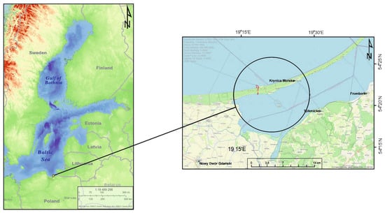
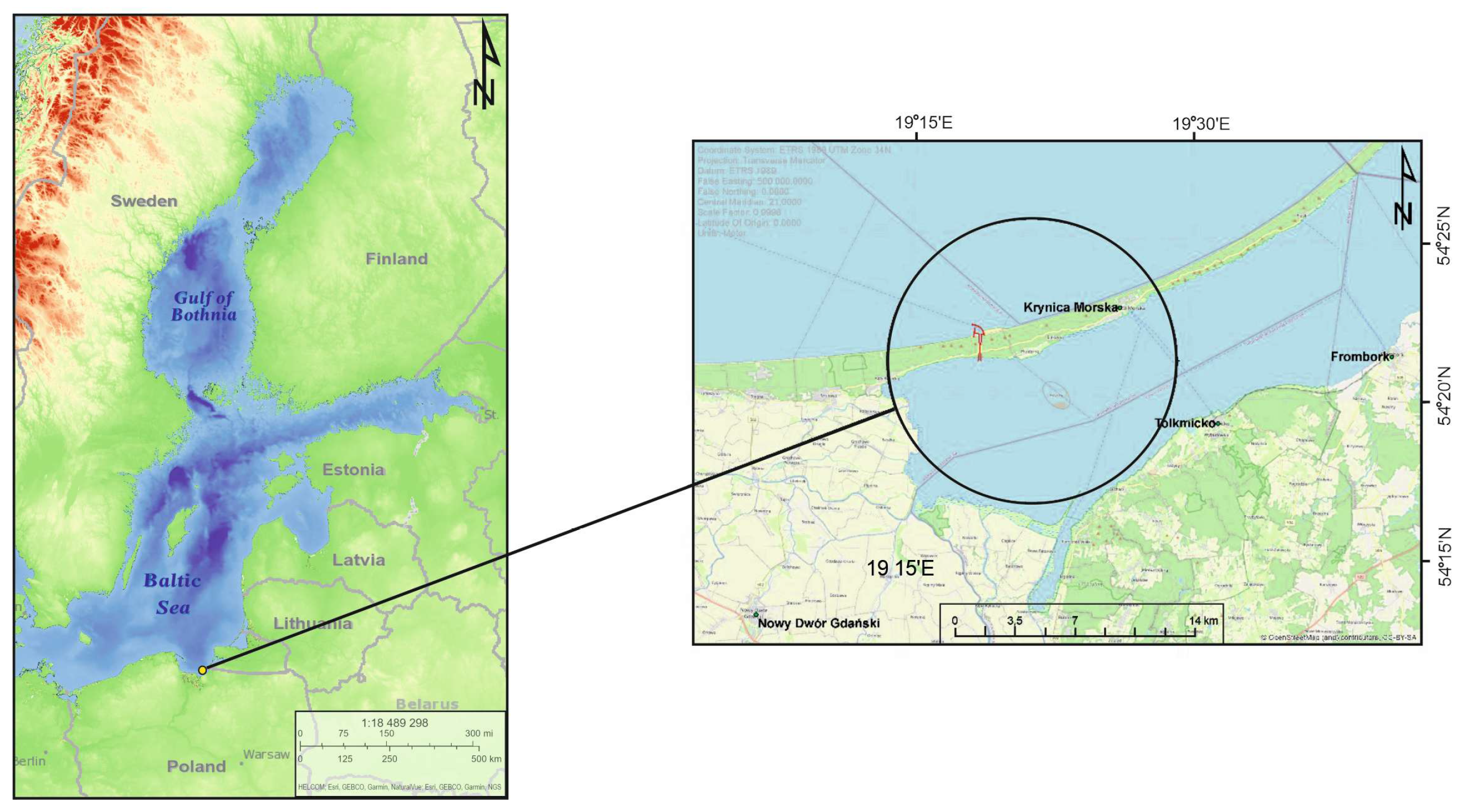
The research area covers a 1.5-km section of the coastline on the Vistula Spit in Poland, in the South Baltic Sea (Figure 1). The Vistula Spit is a naturally formed, sandy geomorphological feature approximately 90 km long and 1–2 km wide, extending from the Pilawa Strait in Russia to Sobieszewska Island in Poland. The Spit is characterized by well-developed coastal dunes, reaching heights of 7 to 12 m and widths of 50 to 100 m (Basiński [17]). The average beach width ranges from 30 to 40 m. Before the Channel was constructed, the section of the coast from the eastern border of Poland to the Vistula Spit Channel represented the longest entirely natural, unurbanized shoreline in the South Baltic Sea. Hydrodynamic processes and beach evolution in this area were undisturbed by engineering structures.

Figure 1. Location of the study site. Left panel: View of the Baltic Sea. Right panel: Close-up (zoom) of the area where breakwaters were constructed and where the large-scale artificial beach nourishment project was carried out using 2.2 million m³ of sediment, creating a beach approximately 450 m wide and 1.5 km long. This is the study area where shoreline position measurements were conducted over a one-year period, with subsequent analysis of their changes.

Below, the characteristics of the analysis area are presented with respect to key features impacting the assessment of coastal evolution. Specifically, the following factors were considered: geological structure, wave climate, characteristics of water levels, longshore sediment transport, breakwater characteristics, and artificial beach nourishment project.

2.1.1. Geology and Morphology of the Study Area

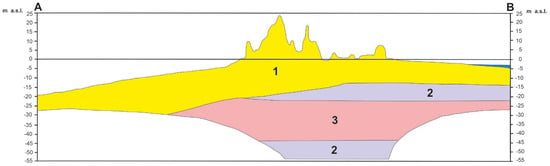
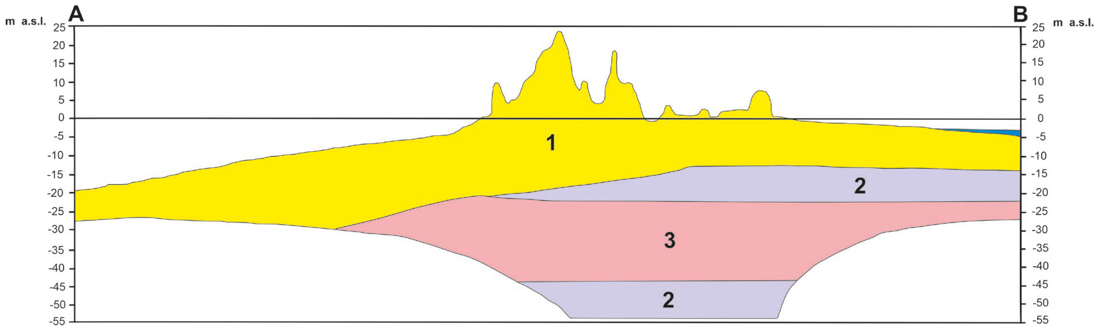
In the geological structure of the Vistula Spit (Figure 2), the mainland part features a layer of Holocene dunes composed of aeolian sands. They stretch along the entire Spit and reach an average height of 10–15 m above sea level and up to 25 m above sea level in the eastern part of the Spit. Below that, there are layers of Holocene sediments (sand, muddy marine sand, beach sand, spit sand, and lagoon sand) with a thickness of about 10–20 m, followed by a layer of clays, silts, and marsh sediments (peat, silt, gyttja, and lake chalk) with a thickness of about 5 m, and a layer of Pleistocene sands with glacial, river, and marine gravels.

Figure 2. Characteristic geological cross-section E–F through the Vistula Spit in the study area. Geological units: 1-aeolian sands forming dunes and sand covers; 3-marine, beach, spit and lagoon sands; 2-clays, silts, lacustrine and fluvial sands, and organic deposits, including peat, mud, gyttja and lacustrine chalk. The cross-section was adapted from the Geodynamic Map of the Polish Baltic Coastal Zone, Sheet 61-Przebrno, State Geological Institute.

2.1.2. Sea Levels

The Baltic is a non-tidal sea. Changes in sea level along the Polish coast above the average level are related to the occurrence of storm surges generated by the impact of wind and barometric pressure on the sea surface. In the analyzed area, storm surges over 50 cm above the average level occur 3–4 times a year, and water levels more than 100 cm above the average level occur at least once every two years. On average, storm surges of 50 cm last about 31–32 h, and those above 80 cm last about 9 h. The standard increase in water level during a storm is 10–16 cm/h, while the maximum is 22 cm/h.

2.1.3. Wave Climate

Szmytkiewicz et al. [18] shows that in the analyzed area, the total period in which waves are generated by winds from offshore directions is about 312 days. Most of the time, waves approach the shore from the north. The highest waves (Hs, max = 4.72 m) also approach from this direction, while the rest approach from the north–northwest (Hs, max = 4.70 m). Waves responsible for longshore sediment transport from west to east come from the northwestern (W–NNW) sector and last a total of 157.86 days per year. Waves from the northeastern sector (N–ENE), which cause longshore sediment transport from east to west, make up a total of 153.81 days. Waves from the W–NNW sector account for approximately 51% of the total time of wave action caused by offshore winds, while waves from the N–ENE sector account for 49%.

2.1.4. Longshore Sediment Transport

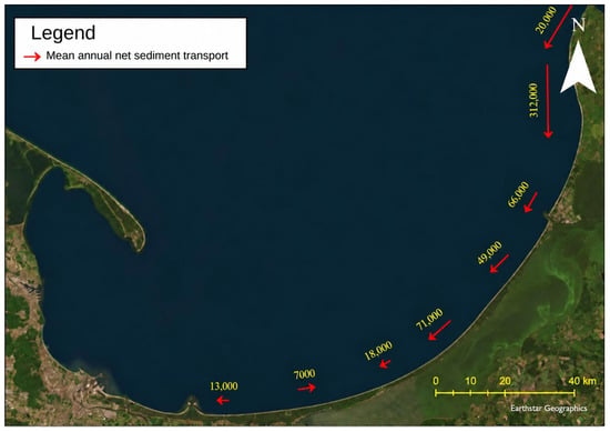
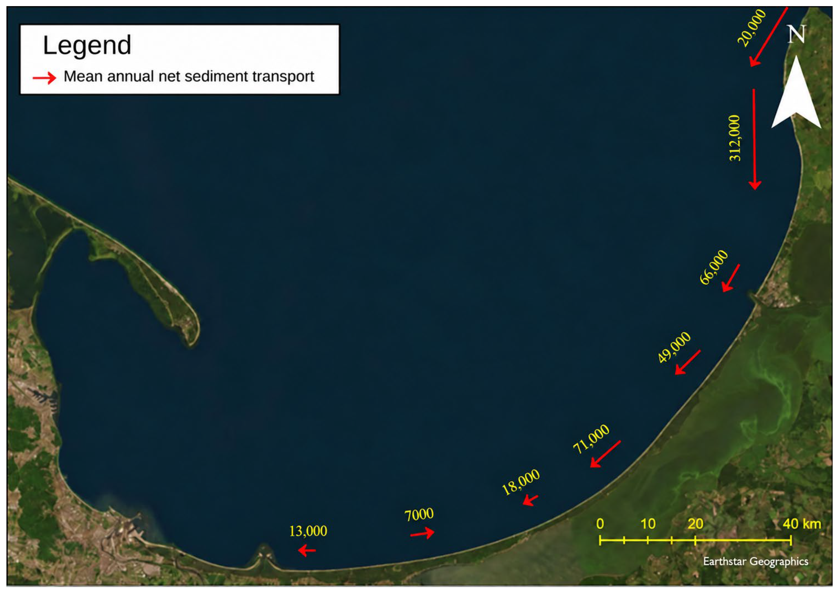
Ostrowski and Kaczmarek [19] presented the mean annual net longshore sediment transport budget across the entire study area. The analysis was based on the methodology described by van Rijn [20]. In this approach, the trigger for longshore sediment transport is the transformation of waves from deep water to the nearshore zone, where wave breaking generates longshore currents, which in turn drive longshore sediment transport. Calculations were performed using multi-year wave data for a single average year, resulting in a long-term (multi-year) mean net longshore sediment transport rate. Figure 2 summarizes the findings of Ostrowski and Kaczmarek [19].

A varied pattern of longshore sediment transport is observed in the study area. Near Yantarny (Russia), the net sediment transport is directed westward and exceeds 200,000 m³ per year. Farther west, toward Poland, the intensity of longshore sediment transport decreases. Near Baltiysk (Russia), it amounts to 70,000 m³/year, while it is only about 20,000 m³/year near Krynica Morska (Poland) (Figure 3). However, the net direction of sediment transport along the stretch between Kąty Rybackie and Krynica Morska is variable. In Kąty Rybackie, transport is directed eastward, whereas in Krynica Morska, it is directed westward. The net annual sediment transport volumes for these locations are 7000 m³/year and –18,000 m³/year, respectively. These directional differences result from the curved exposure of the coastline relative to the deep-water wave climate. In other words, due to processes of refraction and diffraction, the same wave climate in Russia induces westward sediment transport, while in Poland, near the Vistula Spit Channel, the direction is variable and may periodically shift eastward.

Figure 3. The mean annual longshore sediment transport, obtained using the van Rijn (1993) model based on 44 years of wave data, originally presented by Ostrowski and Kaczmarek [19].

2.1.5. Description of the Engineering Project Carried Out Between 2020 and 2022 in the Area of Investigation: Construction of the Vistula Spit Channel and Large-Scale Artificial Beach Nourishment Project

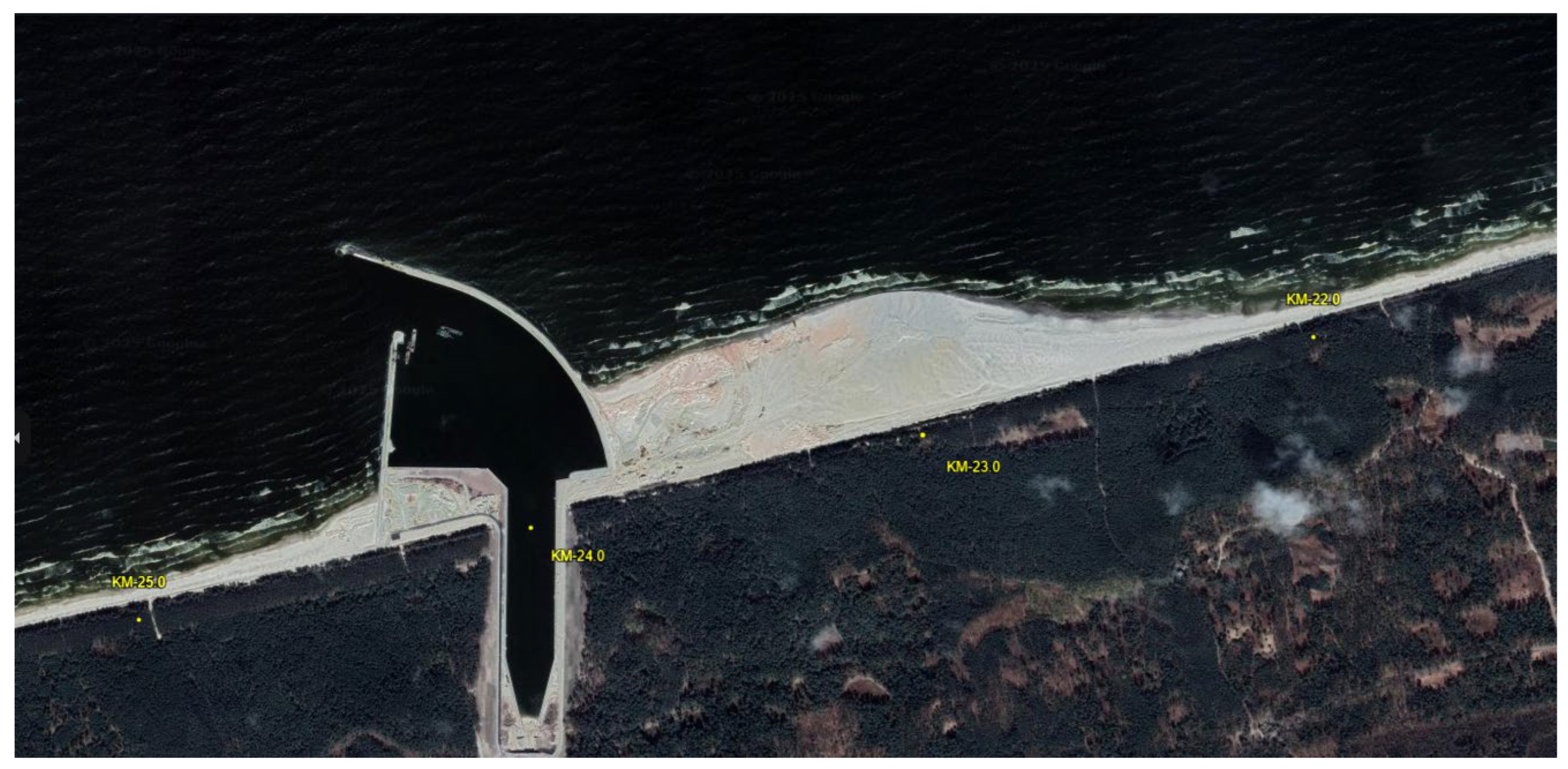
Between 2019 and 2022, the Vistula Spit Channel project was implemented. The channel is 1.5 km long and 5 m deep. On the Gdańsk Bay side, a protective port was constructed, which includes a western breakwater with a length of 568 m and an eastern breakwater with a length of 1014 m, among other structures (Figure 4).

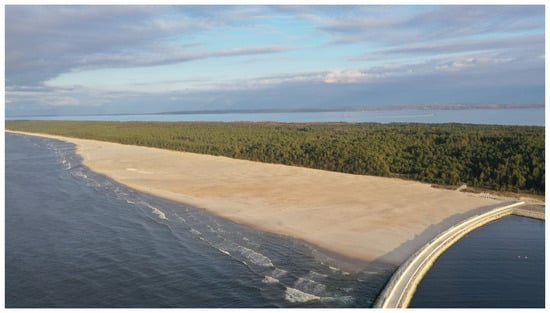
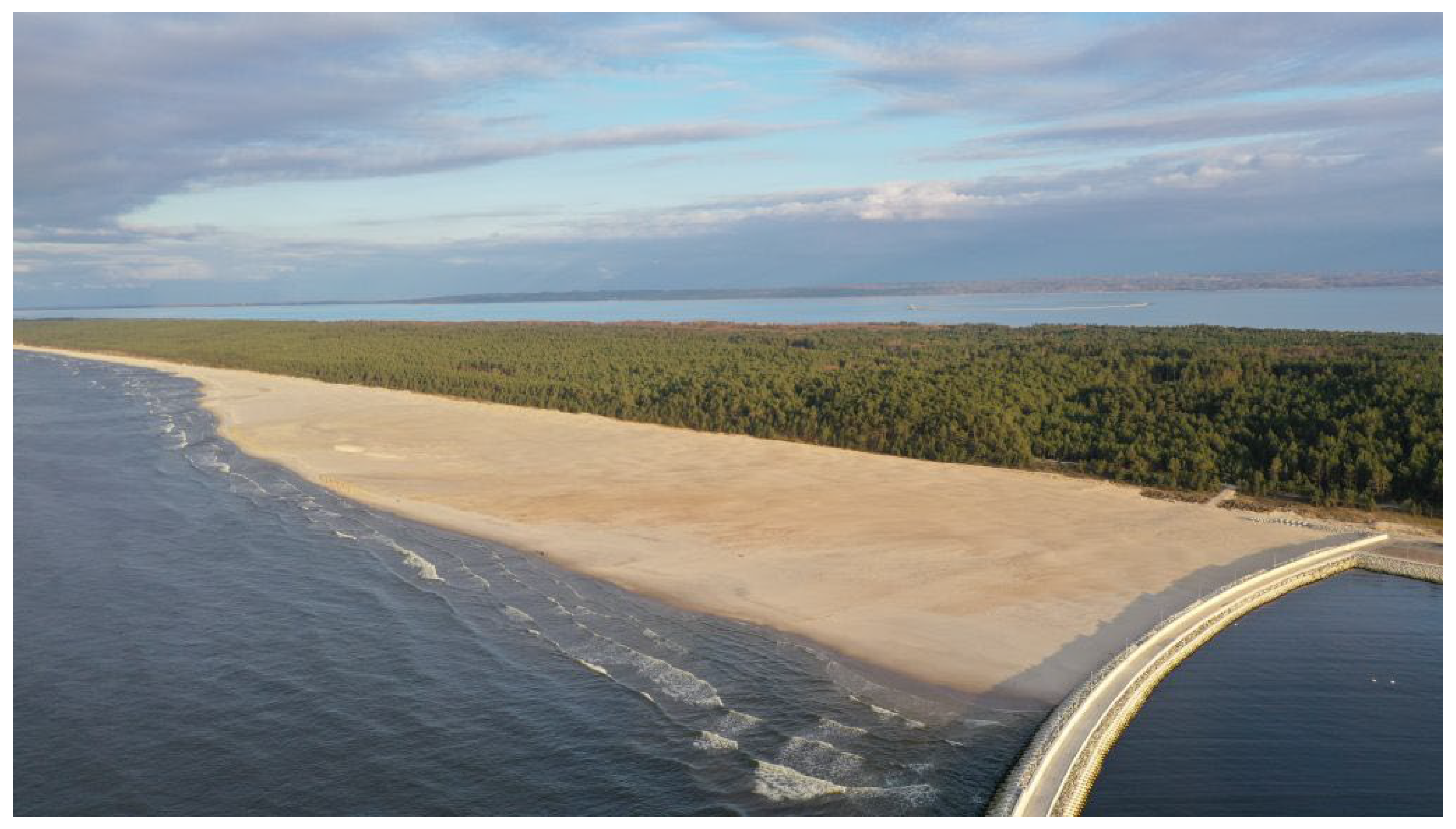
Figure 4. A view of the Vistula Spit Channel port, constructed in 2022. A western breakwater with a length of 568 m; an eastern breakwater extending to 1014 m. Both structures are impermeable breakwaters with a core, armored on the seaward side with Xbloc and XblocPlus units. Large-scale artificial beach nourishment project, 2.2 mln m³ deployed.

During the construction of the Vistula Spit Channel, it became necessary to manage approximately 2.2 million m³ of dredged material. Studies showed that the sand was chemically clean, and the grain size corresponded to sands found on the beaches of the Vistula Spit. During analyses [21], the following factors were taken into account: the resultant average annual sediment transport, the erosive nature of the coast east of the channel, and the possibility of creating a deposit of material for potential future artificial nourishment of the Vistula Spit. Ultimately, the material was deposited east of the eastern breakwater of the Port, as shown in Figure 4 and Figure 5.

Figure 5. View of the large-scale artificial beach nourishment project (2.2 mln m³ of sand) and part of the eastern breakwater. Picture taken in 2022.

2.1.6. Relation to the Sand Motor Concept

The nourished beach investigated in this study can be compared conceptually with the Sand Motor project in the Netherlands, but the two projects are not directly equivalent. Both projects involved the placement of a large volume of sand with the expectation that waves and currents would redistribute the material over time. In both cases, shoreline evolution is therefore controlled not only by the initial geometry of the nourished beach but also by the wave climate, sediment availability, storm events, and longshore transport.

The main difference is that the Sand Motor was intentionally designed as a regional-scale, mega-nourishment experiment aimed at allowing natural redistribution of sand along the adjacent coast. The project investigated here was associated with the construction of the Vistula Spit Channel and the management of approximately 2.2 million m³ of dredged sand. The nourished area is located directly next to an impermeable port breakwater, which creates a stronger local geometric control on wave propagation and sediment transport. The two sites also differ in shoreline orientation, wave climate, sediment characteristics, engineering objectives, monitoring duration, and spatial scale.

Consequently, the Sand Motor provides a useful conceptual reference for post-nourishment sediment redistribution, but it should not be treated as a direct analogue of the present site. The present study focuses on the combined influence of nourishment and a nearby breakwater over a short monitoring period, whereas the Sand Motor literature primarily describes long-term regional redistribution over several years.

2.2. Research Methodology

The data and measurements used in the preparation of this work include the following:

(a)

Analysis of orthophotomaps obtained from the SIPAM website by the Maritime Office in Gdynia and orthophotomaps from the drone survey commissioned by the Institute of Hydro-Engineering of the Polish Academy of Sciences (IBW PAN).

(b)

Hourly wave data from a deep-water point located in front of the Vistula Spit Channel, including wave height, period, and direction. The wave data correspond to the period during which shoreline monitoring was conducted, i.e., February 2024–March 2025.

(c)

Hourly sea-level measurements by tide gauge at the Vistula Spit Channel. The tide-gauge data correspond to the period during which shoreline monitoring was conducted, i.e., February 2024–March 2025.

(d)

Monthly measurements of shoreline position and selected beach-surface elevations used to document beach morphology. Measurements were conducted monthly at approximately 0 cm above average sea level, from February 2024 to March 2025.

Below the sources of individual data, methods for conducting specific field measurements and desk-based analyses are presented.

2.2.1. Analysis of Orthophotomaps

The first stage of this research involved acquiring orthophotomaps available on the SIPAM website, provided by the Maritime Office in Gdynia, as well as orthophotomaps from a drone survey commissioned by the Institute of Hydro-Engineering of the Polish Academy of Sciences (IBW PAN). Using GIS software (ver. 3.4), the coastline was delineated from each available orthophotomap. The shoreline positions were then compared at fixed coastal mileage locations established by the Maritime Office. These locations were used as reference points for describing historical changes in shoreline position between successive observations. The procedure provides information on the alongshore distribution of shoreline change but does not constitute a monthly cross-shore transect analysis.

2.2.2. Wave Data from February 2024 to March 2025

Wave data was obtained from the Copernicus Marine Environment Monitoring Service (CMEMS) and covers the period from February 2024 to March 2025. The selected forecast point is located at a depth of approximately 20 m. The data were processed and analyzed using the Python (3.14, 2025) programming language with libraries such as Pandas, NumPy, Matplotlib, and Seaborn, enabling a detailed analysis of wave directions and heights over time.

2.2.3. Sea Levels (Storm Surges) from February 2024 to March 2025

The data were sourced from the tide gauge operated by the Institute of Meteorology and Water Management (IMGW) installed at the Vistula Spit Channel (on the Gdańsk Bay side) and cover the period from February 2024 to March 2025. The collected measurements were imported into Microsoft Excel spreadsheets, where they were analyzed and visualized in the form of charts.

2.2.4. Monthly Measurements of the Shoreline Position from February 2024 to March 2025

Coastal line measurements were carried out using a satellite GPS RTK device (Real-Time Kinematic), which enables positioning with an accuracy of up to a few centimeters. The measurement began at the point closest to the eastern breakwater and was then conducted along the shoreline. The operator’s movement speed during measurement was approximately 33 m/min, and position registration occurred automatically every 2 s, ensuring high spatial density of points. The total length of the measured shoreline segment was approximately 2 km, extending eastward from the starting point near the eastern breakwater. Unlike the historical data, for which shoreline changes were assessed at fixed coastal mileage locations established by the Maritime Office, the monthly surveys provided continuous shoreline traces along the monitored section. Shoreline changes were analysed using a polygon-based approach for the entire monitored area and in greater detail within two characteristic 250 m sectors: (1) the sector adjacent to the eastern breakwater and (2) the sector located at the eastern boundary of the monitored area. This approach enabled the spatial distribution of erosion and accretion to be identified.

2.2.5. Methodology for Determining the Magnitude of Accumulation and Erosion

The differences in area between successive shoreline positions were calculated using ArcGIS Pro software (CA, USA). The Merge function was first applied to combine multiple shoreline polylines, and then the Feature to Polygon tool was used to generate polygons representing the areas of change between successive shorelines.

This process allows for obtaining the surface area of altered zones in square meters (m²). Based on the geometry and spatial position of the polygons relative to earlier and later shoreline positions, each polygon was manually classified as either representing erosion or accumulation.

The polygon-based method provides the gross area of erosion and the gross area of accretion between two successive shoreline positions. The net area change was calculated as the accreted area minus the eroded area:

Net change = accreted area − eroded area

The method does not resolve the cross-shore displacement of the shoreline at individual alongshore locations. Instead, it quantifies the surface-area balance enclosed between successive shoreline positions. Because erosion and accretion may occur simultaneously in different parts of the monitored section, gross erosion and accretion areas are reported separately from the net balance.

2.2.6. Sector-Based Comparison of Shoreline Change

The monthly shoreline changes were analyzed using two complementary approaches. First, successive shoreline positions were compared over the full monitored coastal section using a polygon-based GIS procedure. This method provided estimates of gross eroded area, gross accreted area, and net area change between consecutive surveys.

Second, the monitored coastline was divided into two characteristic sectors to assess the spatial contrast in shoreline response. The first sector covered approximately 250 m adjacent to the eastern breakwater. The second sector covered an approximately 250 m long section at the eastern boundary of the monitored area. These sectors were selected because the preliminary shoreline mapping indicated contrasting tendencies: a predominantly negative surface balance near the breakwater and a predominantly positive surface balance in the eastern part of the nourished beach.

The sector-based analysis was used to compare the temporal evolution of beach-surface change in the two locations. It does not provide a cross-shore displacement measurement at individual transects. Instead, it describes the net surface balance calculated from shoreline polygons within each predefined coastal sector.

2.2.7. Hydrodynamic

Wave observations were obtained at an offshore point located at an approximately 20–25 m water depth. The designation of this point as a deep-water location requires consideration of the ratio between water depth and wavelength. Because wavelength depends on wave period, water depth alone is insufficient to classify the wave regime. In the present study, the offshore record is therefore treated as a boundary condition representing offshore or relatively deep-water forcing, rather than as a direct measurement of the wave conditions at the shoreline.

During propagation toward the coast, waves may undergo refraction, shoaling, diffraction around the breakwater, partial reflection, breaking, and energy dissipation. These processes modify wave height, direction, period, and the angle of wave approach in the nearshore zone. The breakwater may additionally produce a sheltered zone and a spatial gradient in wave energy, while wave diffraction around the structure may contribute to sediment redistribution near its tip and along the adjacent shoreline.

The interpretation of shoreline change is consequently based on the relationship between offshore hydrodynamic conditions and the observed coastal response. It does not assume that offshore significant wave height is equal to the wave height acting directly at the shoreline.

2.2.8. Definition of Storm Events

For the purposes of this study, a storm event was identified when the significant wave height exceeded 3.0 m at the offshore data point. This threshold is an operational definition used to organize the observations and does not imply that all events produced the same nearshore impact. The duration, direction, associated water level, and antecedent beach condition may influence the morphological response. Water-level exceedance thresholds of 40, 70, and 100 cm above the mean level were analyzed separately and were not treated as interchangeable with the wave-based storm criterion.

2.2.9. Measurement Accuracy and Uncertainty

Shoreline positions were measured using RTK-GPS equipment with centimetre-level nominal positioning accuracy under fixed-RTK conditions. The practical uncertainty of the shoreline position may, however, exceed the nominal instrumental accuracy because of wet-sand conditions, wave run-up, the diffuse land–water boundary, operator movement, and the temporal variability of the beach face. The uncertainty of the GPS measurements was estimated at ±0.031 m.

The drone-based LiDAR data were used to generate digital elevation models and elevation-difference maps. Their interpretation is subject to the vertical and horizontal accuracy of the point cloud, georeferencing quality, point density, surface interpolation, and the presence of water, vegetation, or steep topographic transitions.

Orthophotomap-derived shorelines are affected by image resolution, georeferencing uncertainty, image acquisition date, illumination, water level, wet-sand contrast, and the visual interpretation of the shoreline boundary. Therefore, small changes in shoreline position or area should not be interpreted as geomorphologically meaningful unless they exceed the combined uncertainty of the measurement and shoreline-delineation procedures.

The results are consequently interpreted primarily in terms of persistent spatial patterns and changes substantially larger than the expected measurement uncertainty. The reported uncertainty refers to the measurement and shoreline-delineation procedures and does not represent a formal statistical confidence interval.

According to SIPAM metadata, the 2021–2023 LiDAR datasets had a mean point density of approximately 13 points m⁻², with reported mean horizontal and vertical positional errors of 0.20 m and 0.10 m, respectively. For the 2024 dataset, the mean point density was approximately 8 points m⁻², with reported mean horizontal and vertical errors of 0.50 m and 0.15 m, respectively. These values characterize the accuracy of the source LiDAR data and orthophoto maps from which the products used for shoreline delineation were derived.

For the September and November 2023 datasets from IBW PAN internal materials, we also verified data accuracy using field control points whose coordinates were determined by GNSS measurements. We compared elevation values from the remotely sensed data with corresponding GNSS-derived elevations. Differences ranged from a few millimeters to a few centimeters, with a mean vertical difference of 0.05 m and a maximum observed difference of 0.1 m. Horizontal positional accuracy was of the same order as that reported for the LiDAR datasets used in the study, i.e., approximately 0.20 m. These results indicate centimeter-level vertical agreement and horizontal positional accuracy comparable to the other geospatial datasets used in the analysis.

Shoreline positions derived from these datasets are subject not only to the positional accuracy of the underlying geospatial data but also to uncertainty associated with identifying the land–water boundary. The apparent shoreline position may be affected by water level at the time of data acquisition, wave run-up, wet-sand extent, image contrast, surface interpolation, and the diffuse character of the shoreline boundary. Consequently, the effective uncertainty of the interpreted shoreline position may exceed the nominal horizontal accuracy of the source data.

Therefore, small changes in shoreline position or area should not be interpreted as geomorphologically meaningful when they are comparable to the combined uncertainty of the source data and the shoreline-delineation procedure. Consequently, the results are interpreted primarily in terms of persistent spatial patterns and changes substantially larger than the expected measurement uncertainty. The reported uncertainty refers to measurement and shoreline-delineation accuracy and does not represent a formal statistical confidence interval.

3. Results

3.1. Historical Shoreline Evolution and Topographic Change

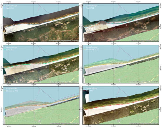
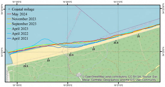
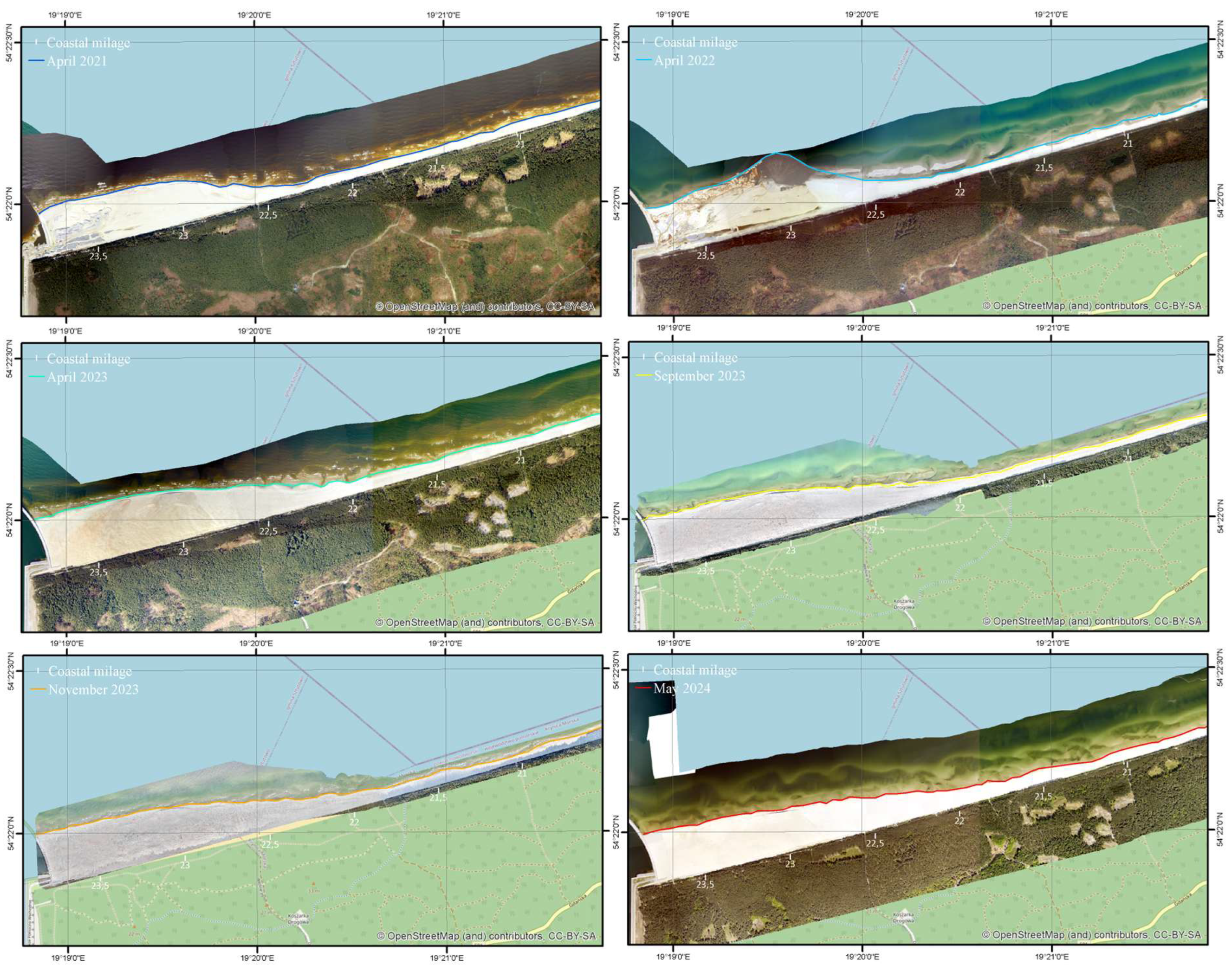
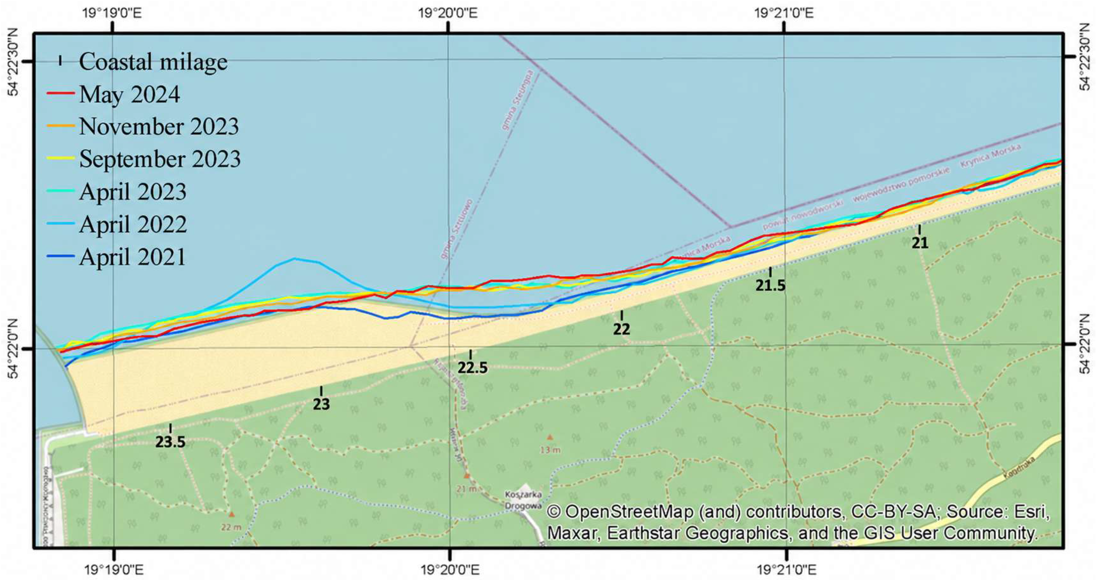
Figure 6 presents changes in the coastline positions obtained from the orthophotomaps in the period of 2021–2024. Upon visual inspection, attention should be drawn to the fact that well-developed dune toe remains unchanged with each subsequent measurement. The most significant changes along the studied section of the coast are observed in the area where beach nourishment was carried out, specifically from the eastern breakwater to approximately KM 22.7. In this region, the coastline is becoming progressively flatter, which has led to an overall widening in the eastern part of the beach. This process is particularly noticeable between KM 22.5 and KM 22, where the beach extension is most evident. The nourishment project substantially modified the shoreline geometry and increased beach width in the eastern part of the study area. The available observations demonstrate shoreline reconfiguration, but they do not by themselves prove that the beach had reached a stable morphological state.

Figure 6. Coastline positions between 2021 and 2024. Data for April 2021, April 2022, April 2023, and May 2024 were obtained from SIPAM (accessed in November 2024). Data for September and November 2023 were obtained from IBW PAN’s internal materials.

Table 1 shows that the most significant changes in the coastline position occurred in 2022, during which beach nourishment works were undertaken. The following period, from April 2022 to April 2023, exhibited the next largest amplitude of coastline changes after the completion of these works. In the subsequent years, the changes were comparatively smaller. From November 2023 to May 2024, a seaward shift in the coastline was observed along nearly the entire length of the studied area, except for the section where beach nourishment was implemented. The segment between KM 21.5 and KM 23 is notably dynamic, with the beach between KM 21.5 and KM 22.5 showing a significant increase in width in 2024 compared to 2021, ranging from 42 to 98 m.

Table 1. Change in shoreline position between 2021 and 2024 along KM 15.0 to 23.5.

KM	April 2021–April 2022 [m]	April 2022–April 2023 [m]	April 2023–September 2023 [m]	September 2023–November 2023 [m]	November 2023–May 2024 [m]	April 2021–May 2024 [m]
16	+2.7	+9.5	−5.8	−3.2	+7.8	+11
17	−1	+3.6	+5.8	−17.6	+9.2	0
18	−15.6	+23.5	−14	+5.8	+9	+8.7
19	+2	+4.5	−15	+4.7	+2.3	−1.5
20	+10	+2	−8.6	−5.4	+15	+13
21	+6	−8.3	−6.4	−8	+18	+1.3
21.5	+12	+3	+6.8	−0.4	+20.6	+42
22	−15.3	+33.8	+8.7	+2.8	+16	+46
22.5	+33	+71	−12.8	−2.7	+9.5	+98
23	+159	−119	−7.5	−12	−25	−4.5
23.5	+31.5	+12.6	−19.6	−2.5	−19	+3

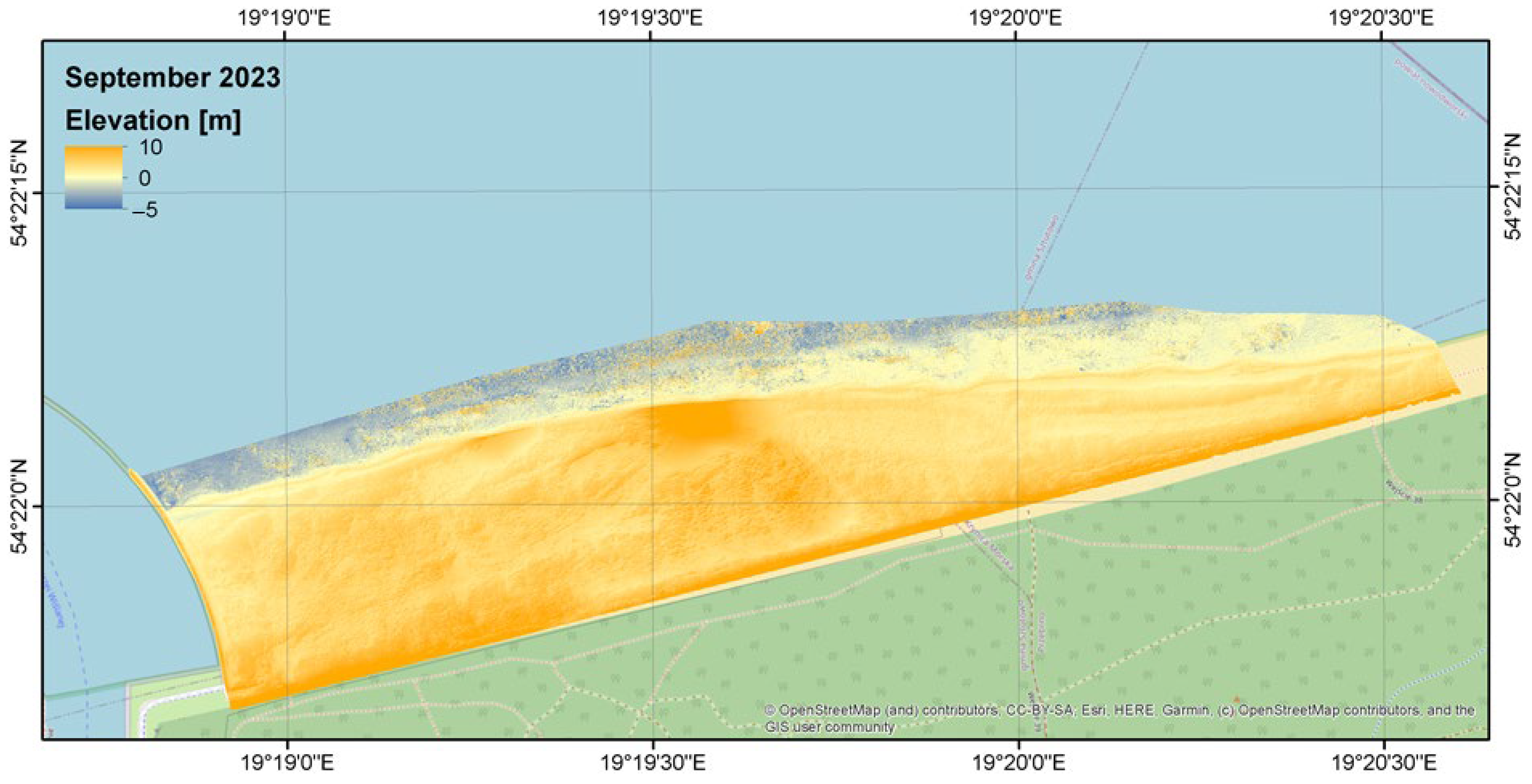
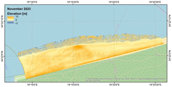
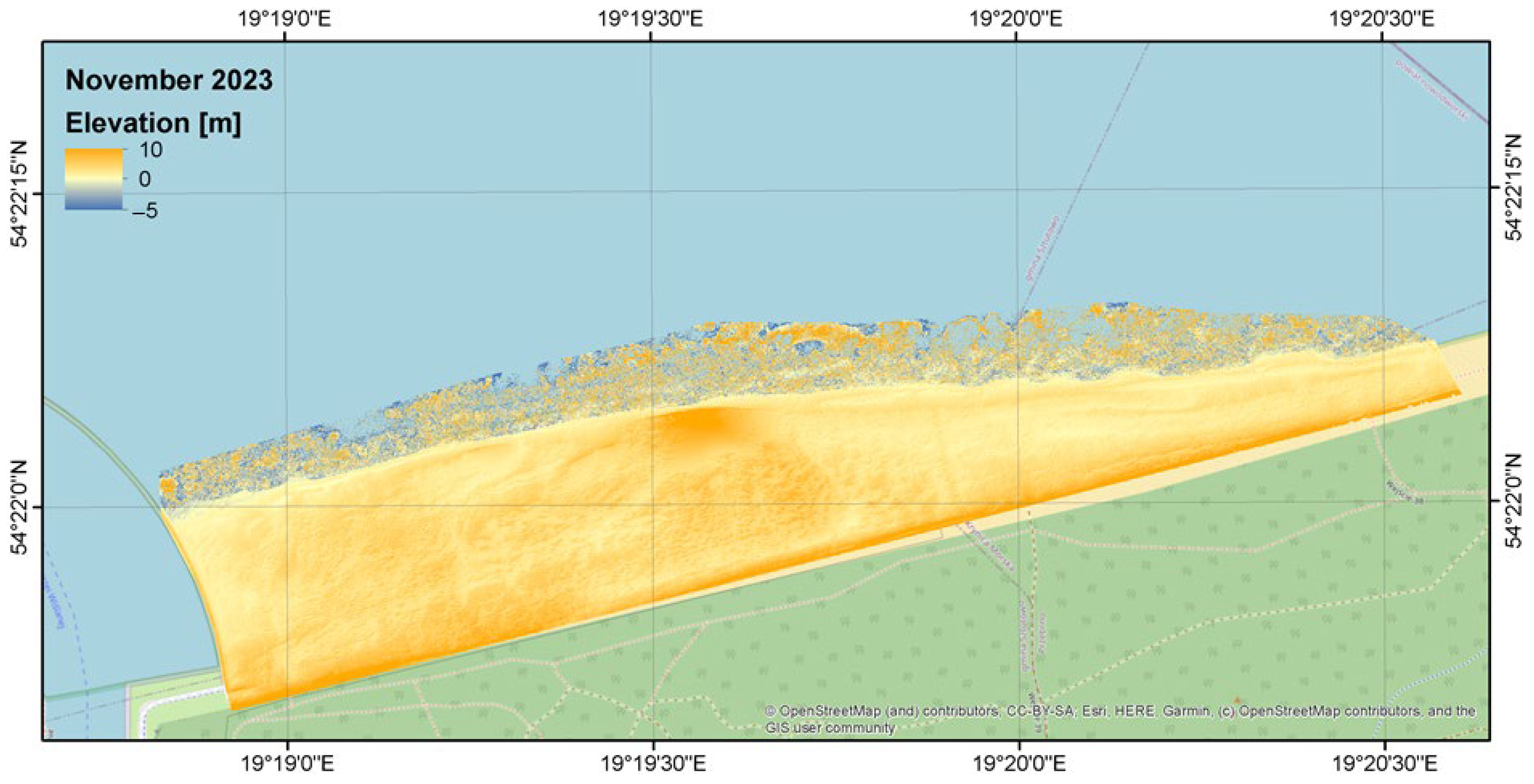
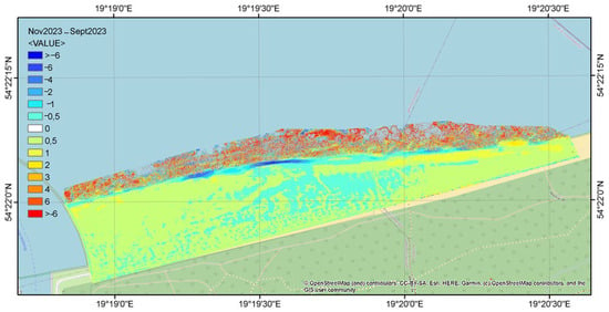
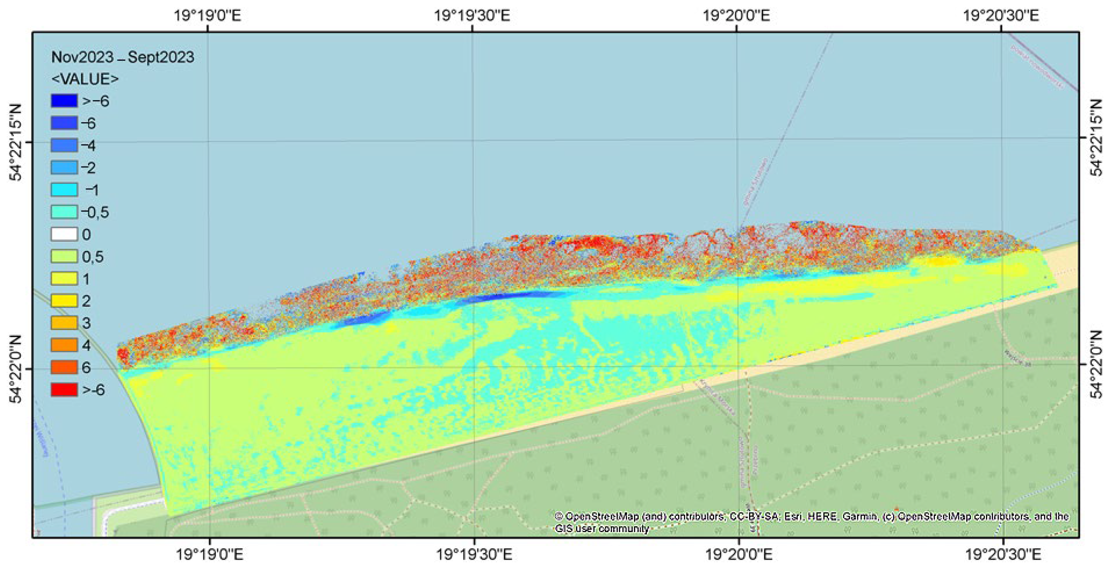
To obtain more precise topographic data, we used LIDAR data collected by the drone to create Digital Elevation Models (DEMs) (Figure 7 and Figure 8). A differential map representing changes in the elevation between these two periods is presented in Figure 9.

Figure 7. Digital Elevation Model of the artificially nourished beach in the vicinity of the Vistula Spit Channel. Measurements were conducted in September 2023.

Figure 8. Digital Elevation Model of the artificially nourished beach in the vicinity of the Vistula Spit Channel. Measurements were conducted in November 2023.

Figure 9. Differential map (November 2023–September 2023) showing changes in the Digital Elevation Model of the artificially nourished beach near the Vistula Spit Channel.

3.2. Offshore Wave Conditions

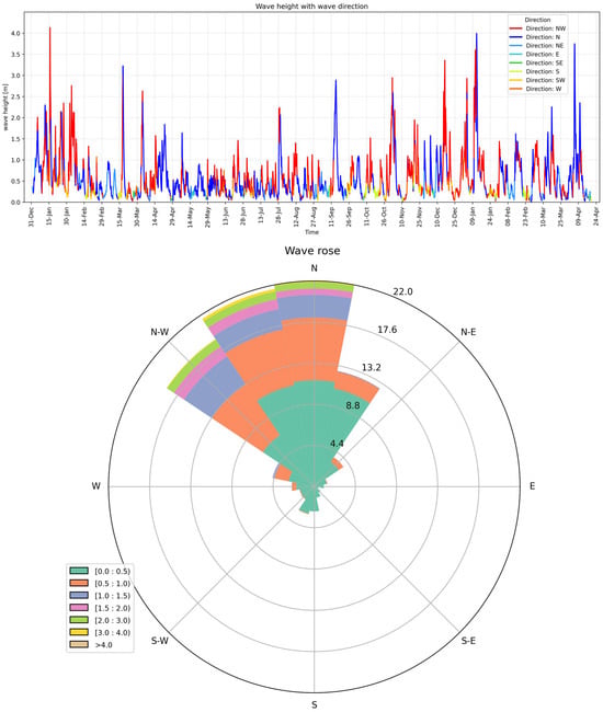
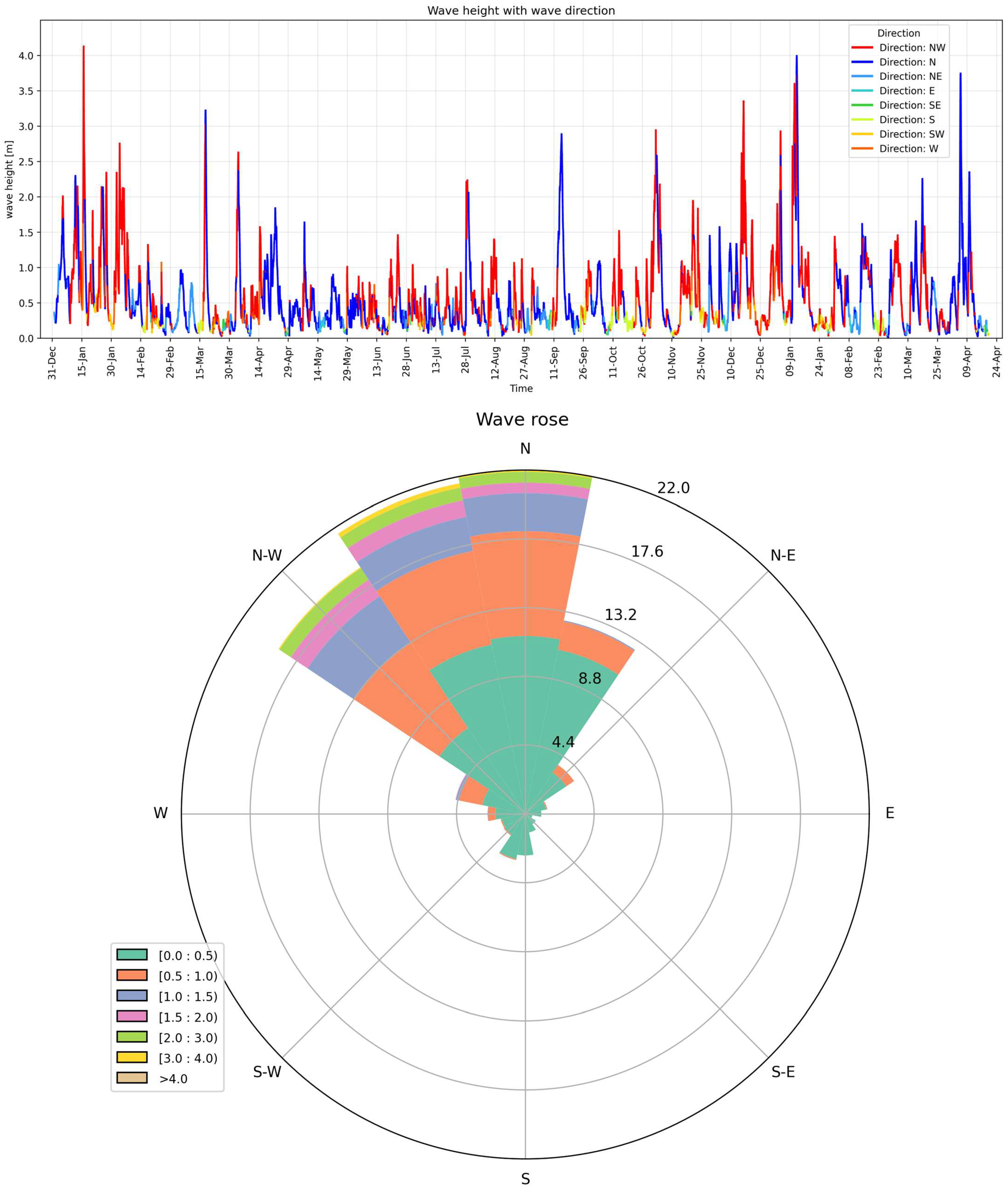
Figure 10 presents significant wave heights and a wave rose for a deep-water point located at a depth of approximately 25 m in front of the analyzed coastal section, covering the entire measurement period from February 2024 to March 2025.

Figure 10. Significant wave heights and wave directions at an offshore wave-data point located at an approximately 20–25 m water depth in front of the analyzed coastal section. The data cover February 2024–March 2025. The offshore record characterizes the general hydrodynamic forcing and does not represent direct nearshore wave conditions.

Based on the collected data, the following conclusions are drawn: Throughout the entire analyzed measurement period (February 2024–March 2025), wave activity was predominantly observed from the NW to N directions. The maximum significant wave height recorded was 4.02 m. During this period, six storm events occurred, with significant wave heights exceeding 3.0 m. During these events, offshore significant wave heights exceeded 3.0 m. Lower values reported for other periods describe the general background wave climate and should not be conflated with the storm maximum. The largest waves were observed between October and January, while the lowest wave activity occurred between April and September. In the period of February–March, waves from the northern sector prevailed, mostly up to 1 m, with maximum values reaching 3 m during inflows from northwestern and northern directions. The largest wave events lasted approximately three days. A noticeable variability in wave directions was observed in the second half of March. Between March and April, the northern direction dominated, with waves mostly reaching up to 1.5 m. The end of March and the period of 7–10 April were characterized by dynamic directional shifts, sometimes occurring multiple times per day. By the end of April, waves from the east prevailed. During these highly variable periods, wave heights did not exceed 0.5 m. In April and May, the northern wave direction was dominant. Waves generally reached up to 1 m, with occasional waves of up to 2 m. Between 14 and 18 May and toward the end of the month, directional variability was observed, shifting between northwestern and eastern. Most waves during these intervals did not exceed 0.5 m. The highest wave, approximately 1.7 m, originated from the northern direction. From May to June, waves from the north–northwestern direction prevailed, typically up to 1 m, and sporadically up to 1.5 m. Waves from outside the main sectors did not exceed 0.5 m. During the June–July period, the north–northwestern direction remained dominant. Waves usually reached up to 1 m, except for the period from 28 to 31 July, when wave heights exceeded 2 m. Increased variability emerged at the end of June, with a dominance of western waves. Waves from less representative directions did not exceed 0.5 m. In July and August, waves most frequently originated from the northern and northwestern directions, with heights of up to 1 m. The highest values were associated with waves from the northwest, while waves from other directions did not exceed 0.5 m. From August to September, the northern direction prevailed. Waves typically reached up to 1 m, with the highest wave recorded between 13 and 16 September, reaching approximately 3 m and originating from the north. Waves outside the dominant sectors had heights below 0.5 m. In September and October, the northern wave direction dominated, with waves generally not exceeding 1 m, except for occasional instances in which they reached up to 1.5 m. After 17 October, the direction stabilized to the south. Wave heights from less dominant directions did not exceed 0.5 m. Between October and December, winds from the north–northwestern and northwestern sectors prevailed. Significant wave heights typically did not exceed 2 m, though they occasionally surpassed this threshold. The highest values were associated with the dominant directions, while waves from other directions did not exceed 0.5 m. From December 2024 to March 2025, wave activity mainly originated from northwestern and north–northwestern directions. Most waves were within the range of up to 1.5 m, occasionally reaching 2–3 m. The maximum recorded significant wave height was nearly 4 m, originating from the northern direction. Waves from non-dominant directions had heights below 0.5 m.

The wave record indicates pronounced seasonal and directional variability. However, the offshore measurements cannot be used as a direct proxy for nearshore wave conditions without accounting for depth-induced transformation and the influence of the breakwater. In particular, wave refraction and shoaling may modify the angle and height of waves approaching the shoreline, while diffraction may redistribute wave energy near the breakwater. The wave record is therefore used here to characterize the timing and general direction of hydrodynamic forcing rather than to calculate the exact wave energy acting at each shoreline segment.

3.3. Sea-Level Variability and Storm-Related Conditions

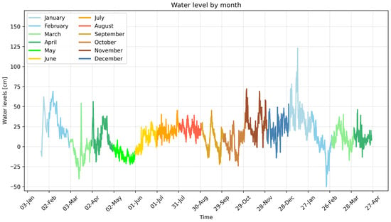
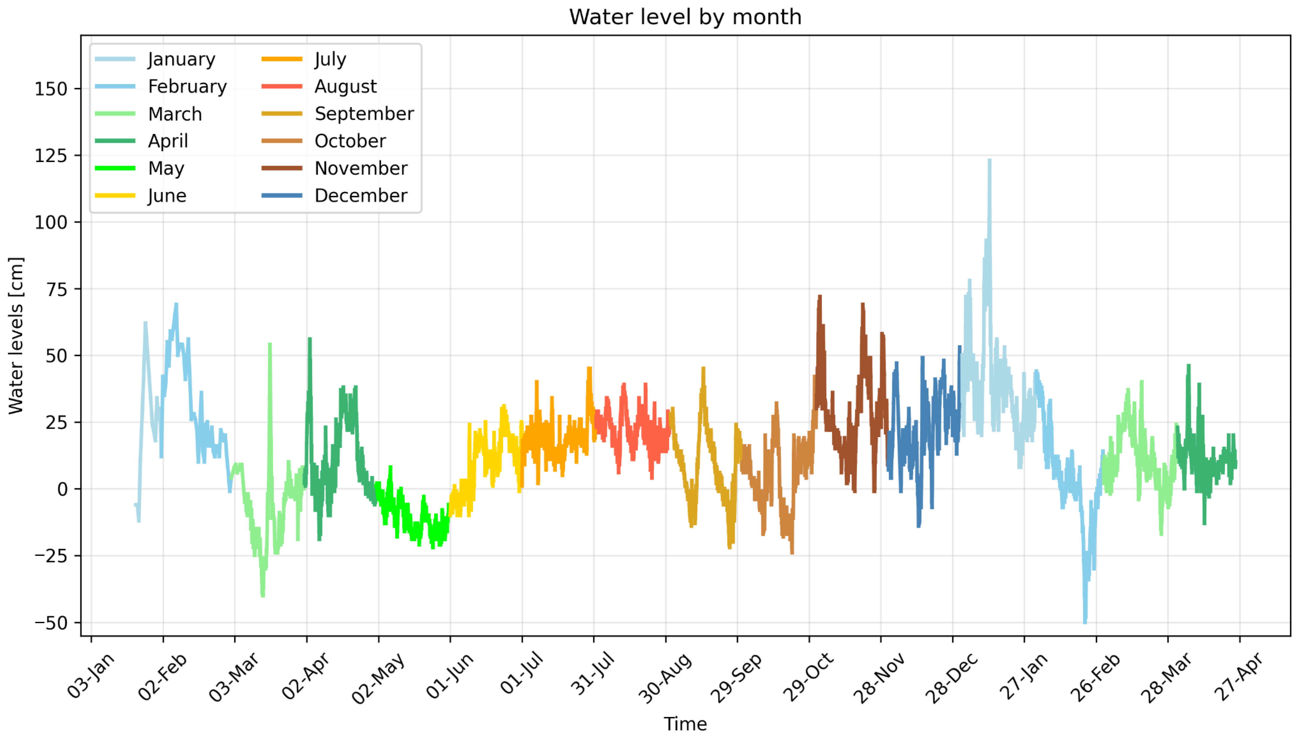
Figure 11 presents hourly sea levels from January 2024 to March 2025. The vertical axis displays sea levels in centimeters above mean sea level, while the horizontal axis indicates measurement dates. To facilitate data analysis, the graph is color-coded by month, denoted with Roman numerals. During the study period, sea levels ranged from −55 cm (55 cm below mean sea level) to 127 cm above sea level. In 2024, values fluctuated between −40 cm and +80 cm. In January and February, sea levels varied between −20 cm and +70 cm, with moderate fluctuations observed. In March, sea levels dropped to −42 cm, followed by a sharp rise to +54 cm. Subsequently, water levels decreased again and gradually increased. In early April, another spike to +63 cm occurred, after which values dropped sharply and then rose again.

Figure 11. Sea levels recorded using a tide gauge installed at the Przekop Mierzei (Vistula Spit Cut) from 21 January 2024 to 4 March 2025 (during the measurement campaign). The vertical axis displays sea levels in centimeters above mean sea level, while the horizontal axis indicates measurement dates. To facilitate data analysis, the graph is color-coded by month, denoted with Roman numerals.

In May, water levels progressively declined, reaching their lowest values in June before rising again. During July and August, sea levels remained relatively stable, oscillating between 0 cm and +50 cm. In September and October, a downward trend dominated, interrupted by three distinct spikes in water levels. In November and December, the trend shifted to an upward direction, culminating in the highest sea level recorded in January 2025 (127 cm). After this peak, water levels began to decline again, reaching the lowest value of −55 cm in late February, followed by another increase. Throughout the study period, daily fluctuations exceeding sea level by tens of centimeters were observed. The smallest variations occurred during summer months, while the largest fluctuations were recorded in the autumn–winter period, coinciding with the storm season. During measurements, the +40 cm threshold (Table 2) was exceeded 75 times, the +70 cm level was recorded 11 times, and the + 100 cm level was observed only twice.

Table 2. Number of events per month with water levels exceeding 40, 70, and 100 cm above the mean level due to storm surge.

Month of the Year	Number of Events Exceeding X cm Above the Mean Water Level
	X = 40 cm	X = 70 cm	X = 100 cm
February 2024	13	3	0
March 2024	1	0	0
April 2024	3	0	0
May 2024	0	0	0
Jun 2024	2	0	0
July 2024	5	0	0
August 2024	1	0	0
September 2024	2	0	0
October 2024	1	0	0
November 2024	12	2	0
December 2024	10	0	0
January 2025	23	6	2
February 2025	2	0	0
March 2025	0	0	0
Total	75	11	2

The sea-level record shows that the monitoring period included both relatively calm intervals and periods of pronounced storm-related water-level variability. The highest recorded level was +127 cm relative to the adopted mean sea level, whereas the lowest value was −55 cm. The occurrence of elevated water levels does not necessarily indicate a uniform shoreline response because the morphological effect depends on the concurrent wave height, wave direction, duration of the event, and local beach morphology.

3.4. Polygon-Based Analysis of Shoreline-Area Change

The monthly shoreline surveys were compared using a polygon-based GIS procedure. The analysis identified the areas enclosed between successive shoreline positions and classified them as erosion or accretion according to the direction of shoreline change. This approach provides a spatially integrated measure of beach-surface change over the monitored coastal section. During the monitoring period, approximately 55,550 m² of erosion and 57,851 m² of accretion were identified. The resulting net change was approximately +2301 m². The positive net balance should not be interpreted as evidence of uniform shoreline stability because the gross eroded and accreted areas were much larger than their difference. The results indicate that substantial erosion and accretion occurred simultaneously in different parts of the monitored area. The polygon-based method therefore provides more information when gross erosion, gross accretion, and net change are considered together.

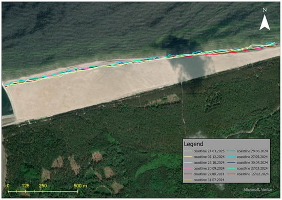
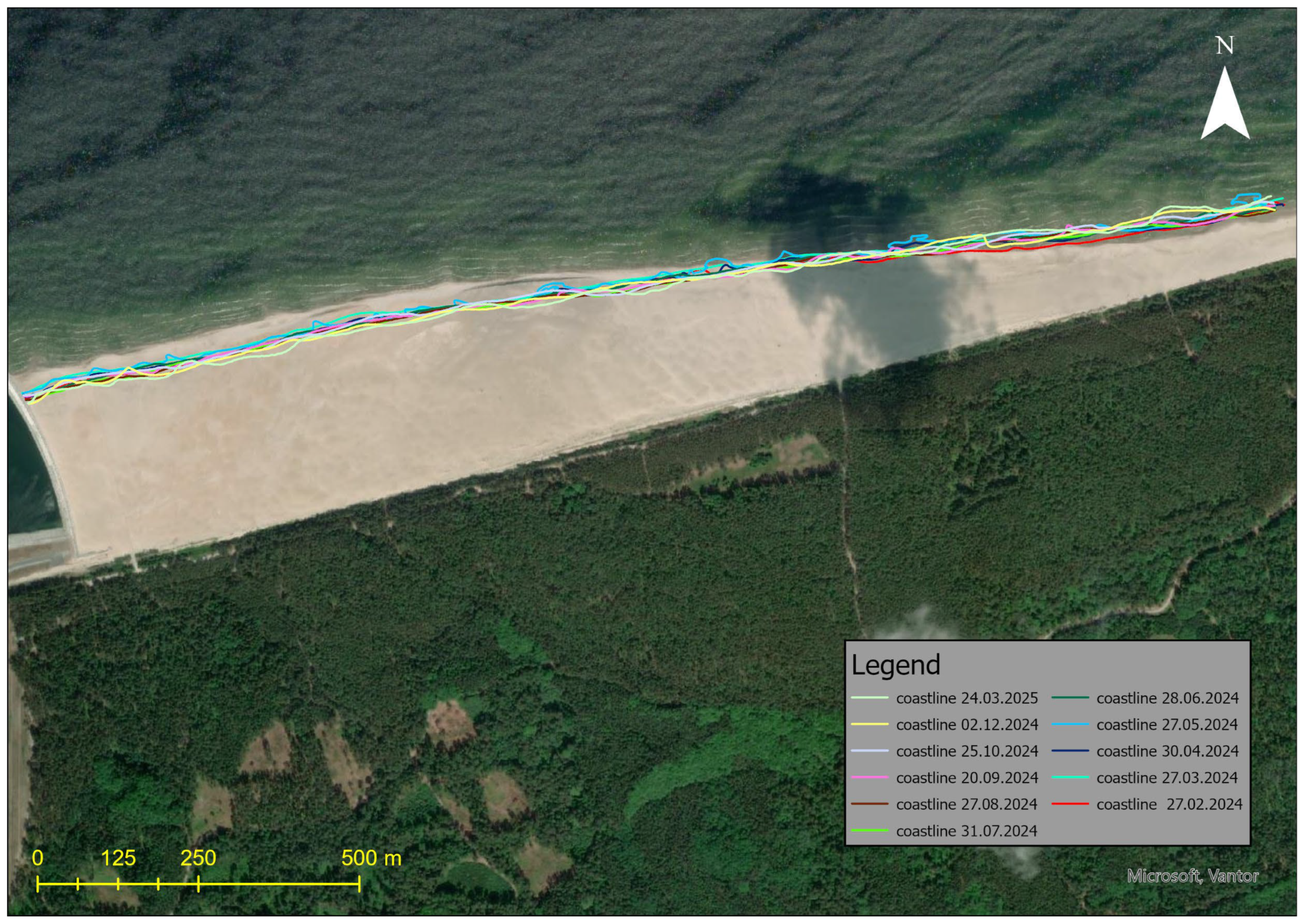
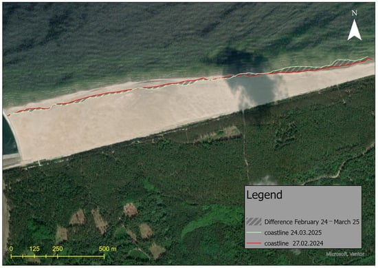
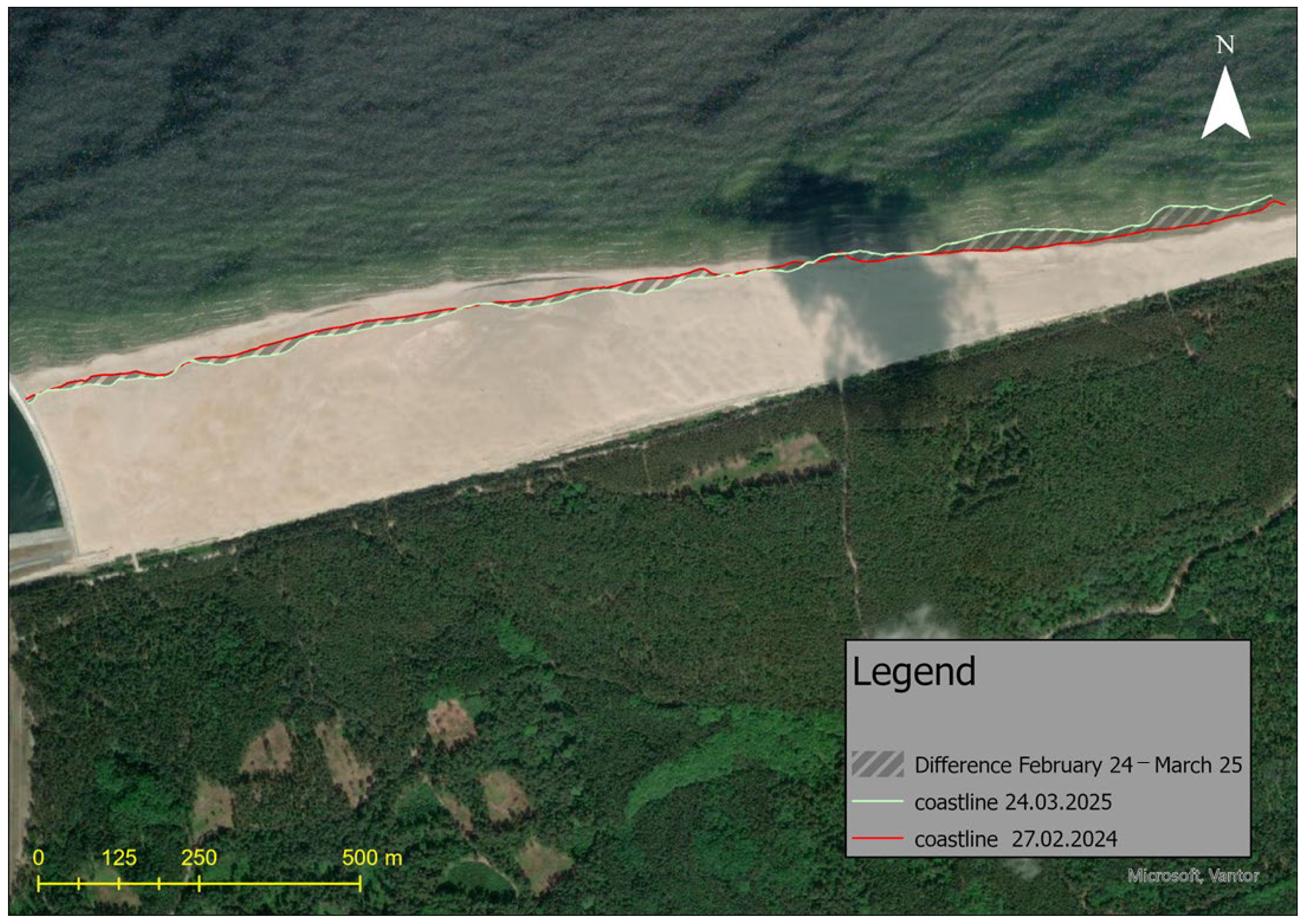
Table 3 presents a summary of changes in the beach area over the entire measurement period along the full length of the studied coastal section, while Figure 12 displays all measurements taken, and Figure 13 shows the shoreline position at the beginning and end of the measurement period (February 2024 and March 2025).

Table 3. Beach surface area difference between shorelines derived from consecutive monthly shoreline position measurements.

Period Between Consecutive Measurements	Eroded Surface of the Beach [m2]	Accreted Area of the Beach [m2]	Net Change [m2]
February 2024–March 2024	−6	20,008	20,002
March 2024–April 2024	−11,973	551	−11,422
April 2024–May 2024	−340	10,602	10,262
May 2024–Jun 2024	−10,962	1336	−9626
Jun 2024–July 2024	−9155	539	−8616
July 2024–August 2024	−1294	3091	1797
August 2024–September2024	−2196	5271	3075
September 2024–October 2024	−2099	7019	4919
October 2024–December 2024	−9415	3925	−5491
December 2024–March 2025	−8110	5509	−2601
Total	−55,550	57,851	2301

Figure 12. Comparison of all shoreline position measurements conducted from February 2024 to March 2025 under the same mean sea-level conditions.

Figure 13. Comparison of example shoreline position measurements taken in March 2025 and February 2024 under the same mean sea-level conditions, with beach accumulation and eroded areas highlighted.

The shoreline changed dynamically but did not shift by more than 35 m. Over the entire measurement period, approximately 55,000 m² of beach area was lost, while about 57,000 m² was gained. Ultimately, the net change is positive—the beach area increased by approximately 2300 m². Detailed analysis reveals that the shorelines from February and March show the largest difference in area between them, yet almost no beach loss occurred between these measurements. The March shoreline is more uniform compared to the February one. The most significant changes are observed in the eastern part of the measured coast and near the breakwater. Between the March and April measurements, a greater loss of beach area was recorded compared to gain. The April shoreline has a similar shape to the March one near the breakwater but is slightly shifted landward. In the eastern section, the shorelines no longer overlap—the March line has a more irregular course. Between April and May, an increase in beach area (which is 10,262) nearly balanced the previous loss from March and April (which is −11,422) (the difference is only 1160 m²). The shapes of the shorelines from these months do not coincide at any point. The May shoreline is highly irregular with numerous inlets compared to the more uniform April line. Between May and June, a loss of beach area occurred. The June measurement shows a more regular shoreline shape compared to May. The most noticeable landward shift was observed near the breakwater and in areas where inlets were present in May. Between June and July, another loss of beach area was recorded. The July shoreline follows a similar course to that of June, with a clear shift landward. In some places, the two lines overlap, while they intersect in the eastern section, resulting in only local gain in the beach area. Between July and August, a slight increase in beach area was recorded, amounting to approximately 1.8 m². The shorelines from these two measurements largely overlap. Near the breakwater, the lines almost perfectly coincide, while the eastern section shows greater differences—this is where the beach area increased. Between August and September, another increase in beach area occurred. The largest gain was recorded near the breakwater, where the shoreline has a more regular shape compared to more distant parts of the same line. The September shoreline is generally more irregular than the August one. Between September and October, another increase in beach area was recorded. The October shoreline is as irregular as the September one, with both lines overlapping only on a short section near the breakwater. Between October and December, a loss of beach area was observed. The December shoreline clearly retreats compared to the October one, except in places where bulges formed, intersecting the previous line. In some segments, these lines overlap. Both are characterized by an irregular course. Between December 2024 and March 2025, a loss of beach area occurred. Both shorelines are irregular and overlap only in a few places, but they do not follow an identical path.

3.5. Sector-Based Comparison of Erosion and Accretion

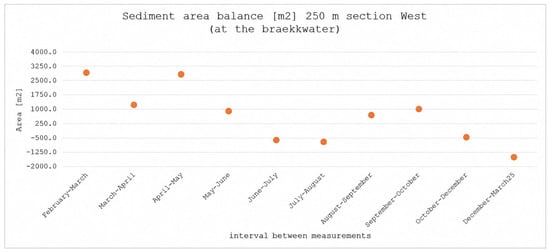
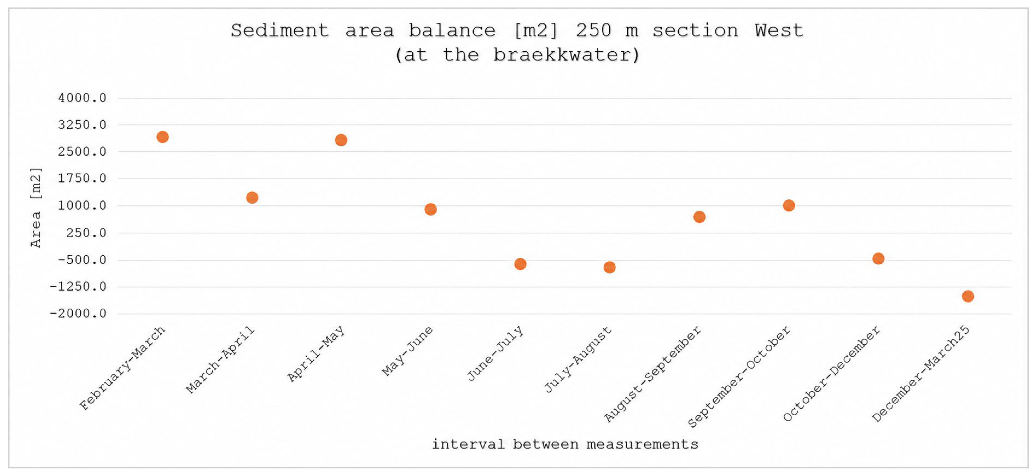
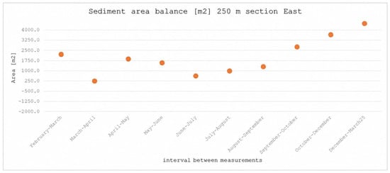
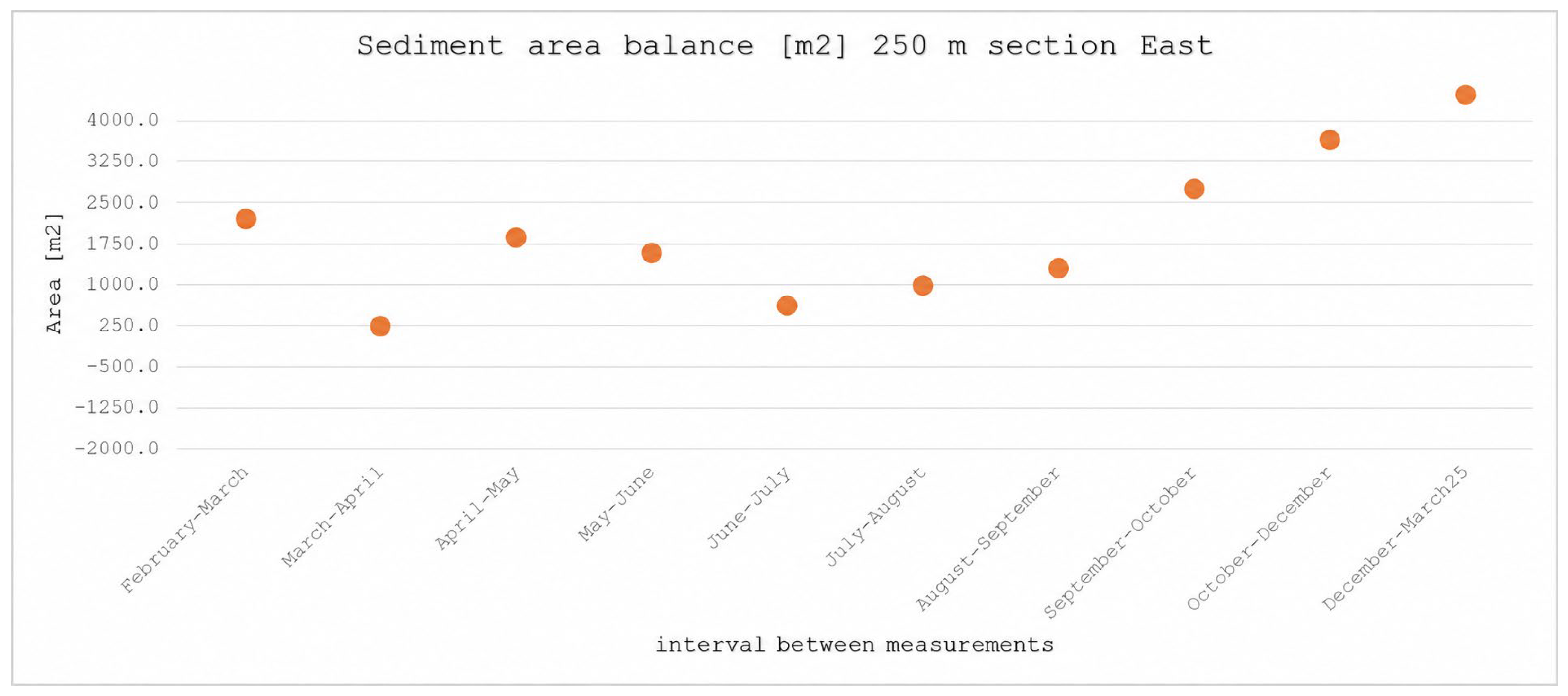
The spatial contrast in shoreline-area change was examined by comparing two predefined coastal sectors. The first sector covers approximately 250 m adjacent to the eastern breakwater, whereas the second sector covers approximately 250 m at the eastern boundary of the monitored area. Figure 14 and Figure 15 present the changes in beach-surface area calculated for these two sectors from successive shoreline polygons.

Figure 14. Changes in beach-surface area within the approximately 250 m sector adjacent to the eastern breakwater, calculated from successive shoreline polygons between February 2024 and March 2025. The points represent successive measurement intervals.

Figure 15. Changes in beach-surface area within the approximately 250 m sector at the eastern boundary of the monitored area, calculated from successive shoreline polygons between February 2024 and March 2025. The points represent successive measurement intervals.

Coastal erosion in the immediate vicinity of the breakwater and accumulation on the eastern side are the most characteristic areas in the discussed case. The first sector is located within 250 m of the eastern breakwater, while the second sub-area covers the eastern part of the studied zone and extends over a 250 m long section at the eastern border of the area. Figure 14 and Figure 15 present the characteristic values of eroded and accumulated beach surfaces in these two sub-areas: the 250 m section east of the Przekop eastern breakwater and the 250 m long coastal section on the eastern side of the analyzed area.

Changes in the shoreline surface in the 250-m section of the western part of the measurements (near the breakwater) are quite dynamic. In this area, there is an almost alternating increase and decrease in the shore. The largest surface increase was recorded between February and March, while the largest decrease occurred between May and June. The general trend of changes in this region indicates a predominant loss of shore surface throughout the entire measurement period, which is also confirmed by the surface balance, indicating a gradual decrease in shore surface in this section.

In the 250-m section of the eastern part of the measurement area, an increase in shore surface was observed throughout the entire measurement period. The largest increase was also recorded in this region between February and March, while the largest decrease occurred between March and April. The shore surface balance for this section shows a trend opposite to that near the breakwater, as the changes exhibit an overall upward trend.

The polygon-based analysis identified approximately 55,550 m² of erosion and 57,851 m² of accretion during the monitoring period, resulting in a net positive difference of approximately 2301 m². This net value is substantially smaller than the gross areas of erosion and accretion and therefore does not indicate that the beach was spatially stable.

The largest erosional response was concentrated near the eastern breakwater, particularly within the approximately 250 m section adjacent to the structure. In contrast, the eastern part of the monitored beach generally exhibited a positive surface balance. This pattern is consistent with the possibility of alongshore sediment redistribution, but it may also reflect the combined effects of the breakwater, wave transformation, initial nourishment geometry, and natural post-nourishment adjustment.

The period from May to June requires particular caution. Although the wave climate was generally less energetic than during the autumn–winter period, the polygon analysis indicates a net loss of approximately 9626 m². This observation demonstrates that low or moderate offshore wave conditions do not necessarily correspond to negligible shoreline change. The response may reflect delayed sediment adjustment, antecedent conditions, local morphological instability, or the effect of wave transformation near the structure.

The results therefore do not support the description of May–June as a uniformly stable period. Instead, the interval should be interpreted as a period of relatively moderate offshore forcing during which substantial local shoreline reorganization nevertheless occurred.

3.6. Interpretation of Shoreline Change in Relation to Hydrodynamic Conditions

The observed shoreline changes occurred during a period characterized by variable wave directions, significant wave heights, and sea levels. The erosion observed near the breakwater and the positive surface balance in the eastern sector indicate that shoreline response was spatially heterogeneous. The available observations do not allow a direct statistical relationship between individual wave parameters and shoreline-area changes to be established. Offshore wave data were used to describe the general timing and direction of hydrodynamic forcing, whereas the shoreline analysis was based on successive shoreline polygons and two predefined coastal sectors. The observed spatial pattern may reflect the combined influence of wave transformation near the breakwater, sea-level variability, the initial geometry of the nourished beach, alongshore sediment redistribution, and delayed post-nourishment adjustment. These processes are discussed as possible explanations of the observations rather than as independently quantified causal relationships.

4. Discussion

4.1. Spatially Variable Shoreline Response

The polygon-based and sector-based results demonstrate that the nourished beach did not evolve as a spatially uniform unit. Erosion was concentrated near the eastern breakwater, whereas accretion was more pronounced in the eastern part of the monitored beach. This pattern is important because the positive net surface balance of approximately 2301 m² could otherwise be interpreted incorrectly as evidence of general beach stability. In reality, the gross values indicate substantial simultaneous erosion and accretion.

The spatial contrast is consistent with the interaction between alongshore sediment transport and the local wave field modified by the breakwater. A breakwater may interrupt sediment pathways, create local gradients in wave energy, and produce zones of diffraction and partial shelter. Nevertheless, the observed pattern cannot be attributed exclusively to the structure because the beach was also undergoing natural adjustment after the placement of 2.2 million m³ of sand.

4.2. Hydrodynamic Forcing and Wave Transformation

The monitoring period included substantial variability in wave direction, significant wave height, and sea level. The predominance of northern and northwestern waves is relevant to the direction of longshore sediment transport, but offshore wave direction does not necessarily correspond to the direction of wave-induced sediment transport at the shoreline. Refraction over the seabed, shoaling, wave breaking, and diffraction around the breakwater may significantly modify the wave angle and energy distribution before waves reach the beach.

Elevated sea levels may increase the water depth over the beach and allow wave energy to act farther landward. However, the response depends on the simultaneous wave conditions and the morphology inherited from previous events. Consequently, a shoreline response observed during a period of moderate offshore waves may reflect the delayed effect of earlier storms or the redistribution of sediment deposited during the nourishment operation.

4.3. Breakwater Effect Versus Post-Nourishment Adjustment

The observed erosional tendency near the breakwater is compatible with a local structural influence, but the available observations do not allow the effect of the breakwater to be separated completely from the natural redistribution of the nourished sand body. The nourished beach was initially far from morphological equilibrium, and sediment could move both alongshore and cross-shore during the monitoring period.

The appropriate interpretation is therefore one of combined forcing. The breakwater likely modified the spatial distribution of wave energy and sediment transport, while the initial nourishment geometry and the natural adjustment of the beach controlled the amount and direction of sediment redistribution. A longer monitoring period, repeated bathymetric surveys, and nearshore wave measurements would be required to quantify the individual contributions of these processes.

4.4. Interpretation of the May–June Interval

The May–June interval should not be described as a period of minimal shoreline variability. Although offshore wave activity was generally lower than during the autumn–winter storm season, the shoreline dataset indicates a net loss of approximately 9626 m². This result shows that shoreline response was not controlled solely by contemporaneous offshore wave height.

Several mechanisms may explain this apparent discrepancy: delayed response to earlier forcing, redistribution of previously accumulated sand, local wave transformation near the breakwater, and the irregular shoreline geometry recorded in May. This observation also demonstrates the importance of comparing hydrodynamic forcing with the spatial distribution of shoreline change rather than relying only on seasonal averages.

4.5. Comparison with the Sand Motor

The present case and the Sand Motor share the general principle that a large placed sand volume is redistributed by natural coastal processes. In both cases, monitoring is required to determine whether sand is retained locally, transported alongshore, or moved offshore.

The two projects differ substantially in purpose and setting. The Sand Motor was designed as a mega-nourishment intended to promote regional sand redistribution over a long period (Huisman et al., [22]). The present project was associated with the construction of a port channel and placed a large volume of dredged sand directly adjacent to an impermeable breakwater. The local structure therefore introduces a stronger control on wave transformation and sediment pathways than in the open nourishment setting of the Sand Motor.

The Sand Motor comparison is thus useful for framing the concept of post-nourishment adjustment but does not demonstrate that the same transport rates, timescales, or shoreline responses should occur at the Vistula Spit site. The main transferable lesson is methodological: large nourishment projects should be monitored using spatially resolved shoreline and bathymetric data over several years, with simultaneous records of waves and water levels.

4.6. Scientific Contribution and Engineering Implications

The principal contribution of this study is the documentation of a short-term, spatially heterogeneous shoreline response following large-scale nourishment adjacent to a newly constructed breakwater. The results demonstrate that a small net shoreline-area change may conceal substantial local erosion and accretion. This finding is relevant to coastal engineering practice because design assessments based only on net sediment volume or total beach area may overlook local erosion hotspots.

The study also emphasizes that offshore wave records should not be interpreted as direct nearshore forcing without considering wave transformation. For engineering applications, monitoring should combine repeated shoreline mapping, polygon-based estimates of gross erosion and accretion, sector-based comparisons, topographic and bathymetric surveys, local or transformed wave data, and water-level observations. Although the one-year observation period does not permit conclusions about long-term equilibrium, the spatial patterns identified here may assist in designing monitoring programs and evaluating nourishment performance at other sites with nearby coastal structures.

4.7. Limitations

This study has several limitations. First, the monitoring period covers approximately one year and is therefore too short to characterize the complete morphological response of the nourished beach. Second, offshore wave data were used to describe the incident wave climate, but nearshore wave transformation was not calculated explicitly. Third, the analysis does not fully separate the effects of the breakwater from the natural adjustment of the nourished sand body. Fourth, the monthly shoreline data were analyzed using polygon-based area calculations and sector-based comparisons rather than a complete cross-shore transect framework. Consequently, the results quantify spatially integrated surface-area changes but do not provide local cross-shore displacement values for individual alongshore locations. Fifth, the study does not quantify a direct statistical relationship between individual hydrodynamic parameters and shoreline-area change. The interpretation is therefore observational and process-based rather than predictive. Finally, the uncertainty associated with shoreline delineation, RTK-GPS positioning, LiDAR-derived elevation models, and orthophotomap interpretation limits the significance of very small reported changes.

5. Conclusions

This study presented an empirical analysis of the short-term evolution of a large artificially nourished beach located adjacent to the eastern breakwater of the Vistula Spit Channel. The analysis combined historical orthophotomaps, monthly RTK-GPS shoreline surveys, drone-based LiDAR data, offshore wave observations, and tide-gauge measurements.

The main conclusions are as follows:

• Shoreline change was spatially heterogeneous. Erosion was concentrated near the eastern breakwater, whereas accretion was more pronounced in the eastern part of the monitored beach.
• The net surface balance does not describe the complete morphological response. Approximately 55,550 m² of erosion and 57,851 m² of accretion were identified, resulting in a net positive difference of approximately 2301 m². This small net value masks much larger opposing changes occurring in different coastal sectors.
• The polygon-based method provides complementary information through the separate reporting of gross erosion, gross accretion, and net change. The sector-based comparison further shows that the same monitoring interval may include erosion near the breakwater and accretion in the eastern part of the nourished beach.
• Hydrodynamic forcing and shoreline response were linked through several interacting mechanisms. Wave direction, wave magnitude, wave duration, sea-level variability, storm events, breakwater-induced wave transformation, and post-nourishment adjustment may all have contributed to the observed changes.
• Offshore wave parameters cannot be treated as direct nearshore forcing. Waves may undergo refraction, shoaling, diffraction, breaking, reflection, and energy dissipation between the offshore data point and the shoreline.
• The May–June interval was not uniformly stable. Although offshore wave activity was generally lower than during the autumn–winter period, a net loss of approximately 9626 m² was recorded. This result indicates that local morphology and delayed sediment redistribution influenced the shoreline response.
• The effect of the breakwater cannot be fully separated from natural post-nourishment adjustment using the present dataset. The observed erosion near the structure is consistent with a structural influence, but longer-term monitoring and nearshore hydrodynamic data are required to quantify its contribution.
• The main scientific contribution is observational and methodological. The study demonstrates how polygon-based shoreline mapping and sector-based comparison can identify simultaneous erosion and accretion on different parts of a large nourished beach adjacent to a breakwater. The results also show why a small net area change should not be interpreted as evidence of uniform beach stability.
• The one-year monitoring period limits interpretation of long-term morphological behavior. Continued monitoring should include repeated shoreline mapping, topographic and bathymetric surveys, water-level observations, and wave data transformed to the nearshore zone. Sector-based and polygon-based analyses should be repeated over several years to determine whether the observed spatial contrast persists.

References

- Short, A.D. Three dimensional beach-stage model. J. Geol. 1979, 87, 553–571. [Google Scholar] [CrossRef] [Scilit]
- Wright, L.D. Beach cut in relation to surf-zone morphodynamics. In Proceedings of the 17th International Conference on Coastal Engineering, Sydney, Australia, 23–28 March 1980; pp. 978–996. [Google Scholar]
- Sunamura, T. A laboratory study of offshore transport of sediment and a model for eroding beaches. In Proceedings of the 17th International Conference on Coastal Engineering, Sydney, Australia, 23–28 March 1980; pp. 1051–1070. [Google Scholar]
- Rudowski, S. Sedimentary environment at the barred coast of a tideless sea; Southern Baltic, Poland. Stud. Geol. Pol. 1986, 87, 1–76. [Google Scholar]
- Furmańczyk, K. Współczesny Rozwój Strefy Brzegowej Morza Bezpływowego w Świetle Badań Teledetekcyjnych Południowych Wybrzeży Bałtyku; Uniwersytet Szczeciński: Szczecin, Poland, 1994; p. 149. [Google Scholar]
- Kraus, N.C. Beach change modeling and the coastal planning process. In Coastal Zone ‘89: Proceedings of the Sixth Symposium on Coastal and Ocean Management; ASCE: Reston, VA, USA, 1989; pp. 553–567. [Google Scholar]
- Larson, M.; Kraus, N.C. SBEACH: Numerical Model for Simulating Storm-Induced Beach Change. Report 1: Empirical Foundation and Model Development; U.S. Army Engineer Waterways Experiment Station: Vicksburg, MS, USA, 1989. [Google Scholar]
- Reeve, D.E.; Fleming, C.A. A statistical-dynamical method for predicting long-term coastal evolution. Coast. Eng. 1997, 30, 259–280. [Google Scholar] [CrossRef] [Scilit]
- Dastgheib, A. Long-Term Process-Based Morphological Modeling of Large Tidal Basins; CRC Press/Balkema: Leiden, The Netherlands, 2012; p. 179. [Google Scholar]
- Guo, L. Modeling Estuarine Morphodynamics Under Combined River and Tidal Forcing (UNESCO-IHE Ph.D. Thesis); CRC Press/Balkema: Leiden, The Netherlands, 2014; p. 214. [Google Scholar]
- Huang, W.P. Modelling the effects of typhoons on morphological changes in the Estuary of Beinan, Taiwan. Cont. Shelf Res. 2017, 135, 1–13. [Google Scholar] [CrossRef] [Scilit]
- Benedet, L.; Dobrochinski, J.P.F.; Walstra, D.J.R.; Klein, A.H.F.; Ranasinghe, R. A morphological modeling study to compare different methods of wave climate schematization and evaluate strategies to reduce erosion losses from a beach nourishment project. Coast. Eng. 2016, 112, 69–86. [Google Scholar] [CrossRef] [Scilit]
- Karathanasi, F.E.; Belibassakis, K.A. A cost-effective method for estimating long-term effects of waves on beach erosion with application to Sitia Bay, Crete. Oceanologia 2019, 61, 276–290. [Google Scholar] [CrossRef] [Scilit]
- Knaapen, M.; Joustra, R. Morphological acceleration factor: Usability, accuracy and run time reductions. In Proceedings of the XIXth TELEMAC-MASCARET User Conference, Oxford, UK, 18–19 October 2012. [Google Scholar]
- Malliouri, D.I.; Petrakis, S.; Vandarakis, D.; Moraitis, V.; Goulas, T.; Hatiris, G.A.; Kapsimalis, V. A chronology-based wave input reduction technique for simulations of long-term coastal morphological changes: An application to the beach of Mastichari, Kos Island, Greece. Water 2023, 15, 389. [Google Scholar] [CrossRef] [Scilit]
- Ranasinghe, R.; Swinkels, C.; Luijendijk, A.; Roelvink, D.; Bosboom, J.; Stive, M.; Walstra, D. Morphodynamic upscaling with the MORFAC approach: Dependencies and sensitivities. Coast. Eng. 2011, 58, 806–811. [Google Scholar] [CrossRef] [Scilit]
- Basiński, T. Ocena Stanu Zabezpieczenia Brzegów Morza Bałtyckiego od Strony Otwartego Morza oraz Zatok Gdańskiej i Puckiej; Raport Made by Request of Maritime Office in Gdynia; Instytut Meteorologii i Gospodarki Wodnej–Państwowy Instytut Badawczy: Warsaw, Poland, 2007. [Google Scholar]
- Szmytkiewicz, M. Wpływ Sztormów na Zmiany Morfologii Brzegu Morskiego na Przykładzie Wybrzeża w Rejonie Władysławowa; Instytut Budownictwa Wodnego PAN: Gdańsk, Poland, 2003. [Google Scholar]
- Kaczmarek, L.M.; Ostrowski, R.; Szmytkiewicz, M. Sediment transport issues related to a planned cross-cut through the Vistula Spit, Poland. Arch. Hydro-Eng. Environ. Mech. 2010, 57, 119–137. [Google Scholar]
- Van Rijn, L.C. Principles of Sediment Transport in Rivers, Estuaries and Coastal Seas; Aqua Publications: Blokzijl, The Netherlands, 1993. [Google Scholar]
- Ostrowski, R.; Pruszak, Z.; Skaja, M.; Szmytkiewicz, M. Variability of hydrodynamic and lithodynamic coastal processes in the east part of the Gulf of Gdańsk. Arch. Hydro-Eng. Environ. Mech. 2010, 57, 139–153. [Google Scholar]
- Huisman, B.J.A.; de Schipper, M.A.; de Vries, S.; van Gelder-Maas, C.; van Thiel de Vries, J.S.M.; Stive, M.J.F. Ten years of Sand Motor: A critical review of its performance and impacts. Coast. Eng. J. 2021, 63, 91–109. [Google Scholar]
Disclaimer/Publisher’s Note: The statements, opinions and data contained in all publications are solely those of the individual author(s) and contributor(s) and not of MDPI and/or the editor(s). MDPI and/or the editor(s) disclaim responsibility for any injury to people or property resulting from any ideas, methods, instructions or products referred to in the content. |
© 2026 by the authors. Licensee MDPI, Basel, Switzerland. This article is an open access article distributed under the terms and conditions of the Creative Commons Attribution (CC BY) license.