


Abstract
Aquifer storage and recovery (ASR) wells along northern Lake Okeechobee, Florida, have been proposed as part of the Comprehensive Everglades Restoration Plan. However, researchers have linked elevated concentrations of As, Hg and transition metals in groundwater because of ASR in carbonate rocks. This study presents portable X-ray fluorescence (pXRF) analyses of four continuous cores (C38S, C59, L63N, and L63S) recovered from the Floridan Aquifer System north of Lake Okeechobee, Florida. A total of 5078 pXRF measurements were collected at approximately 30.5 cm along the four cores. Measurements along the cores included the Intermediate Confining Unit, Upper Floridan Aquifer (UFA), Avon Park Permeable Zones (APPZ), and portions of the Lower Floridan Aquifer (LFA). Emphasis was placed on the concentrations of mercury (Hg), arsenic (As), molybdenum (Mo), chromium (Cr), and nickel (Ni), which have been identified as elements of concern during ASR operations. Major-element trends in the cores often reflect lithologic changes in the Floridan Aquifer System. This includes decreases in Ca and Sr and increases in Mg associated with dolomitization in the Avon Park Formation. Trace-metal concentrations vary systematically within hydrostratigraphic units. Mercury commonly exhibits elevated concentrations near the base of the UFA, whereas Mo is often enriched near the top of the UFA. Elevated concentrations of Hg, As, Mo, Ni, and other trace metals frequently occur at hydrostratigraphic boundaries, formation contacts, clay-rich intervals, and especially within organic-rich layers. Organic layers contained metal concentrations several times greater than surrounding carbonate rocks and hosted the highest measured concentrations of Hg, As, and Mo in the cores. The paucity of organic layers and generally lower metal concentrations in the UFA suggest it may represent a favorable zone for ASR storage. In contrast, the APPZ and LFA contain numerous metal-enriched organic layers which may increase the potential for trace metal mobilization during ASR operations. These results suggest pXRF characterization provides an effective tool for geochemical characterization of storage zones and evaluating water-quality risks potentially associated with ASR development.
1. Introduction
1.1. Overview of Lake Okeechobee Watershed Restoration Project Aquifer Storage and Recovery Wells
The Comprehensive Everglades Restoration Plan (CERP) has included aquifer storage and recovery (ASR) since its conception [1,2]. Upon review by a committee from the National Academy of Sciences, a more comprehensive study was recommended, which included assessing aquifer hydraulic capacity, hydraulic fracturing, and potential water chemistry interactions between the aquifer matrix and the injected and stored water, a committee formed by the National Academy of Sciences reviewed the plan again and found flaws; however, some additional research, particularly regarding water quality, was recommended [3]. The National Research Council (NRC) also recommended a phased approach for developing the regional ASR facilities. The South Florida Water Management District (SFWMD) and U.S. Army Corps of Engineers (USACE) revised the ASR Science Plan based on recommendations from the NRC and a review by an Independent Peer Review Science Panel [4,5].
In the Science plan, the SFWMD provided an analysis to address any remaining ASR uncertainties. The first phase of the ASR well construction and testing was to be located north of Lake Okeechobee (Figure 1). Among the objectives of the project was to provide a comprehensive assessment of the geology and hydrogeology by collecting five continuous cores starting near the base of the intermediate confining unit (ICU), extending through the Upper Floridan Aquifer (UFA), and extending into the Lower Floridan Aquifer (LFA). The number of continuous cores was reduced from five to four during reevaluation of the site locations and budget optimization and to reduce the overall footprint of this ASR project. During the aquifer characterization, Rahman [6], Alvarez [7], Tipton et al. [8], and Dawsy [9] reported detailed chemical analyses of the rock matrix, emphasizing the trace-element chemistry issues (e.g., metal mobilization) which were previously addressed regarding naturally occurring metals such as arsenic, cadmium, lead, mercury, and molybdenum [10,11,12,13]. Carbonate rock geochemistry is a necessary part of the aquifer system characterization because trace metals can mobilize into the groundwater during ASR operation. A detailed analysis of the continuous core matrix geochemistry using a calibrated portable X-ray Fluorescence (pXRF) unit was completed in this research. This paper provides the findings of the pXRF analyses of the continuous cores collected from four ASR sites: C38S, C59, L63N, and L63S. These data were initially reported by MacDonald et al. [14] for L63N and MacDonald et al. [15] for C38S, C59, and L63S as reported to the South Florida Water Management District.
Figure 1.
North Lake Okeechobee ASR well cluster sites [5,6,7,8,9]. The locations of the cores studied for this report (C38S, C59, and L63S) are denoted by red circles on the figure above. MC = Mosquito Creek; NS = Nubbin Slough; TC = Taylor Creek.
1.2. ASR for Water Storage Including the Suwannee Limestone, Ocala Limestone, and the Avon Park Formation
In Florida, ASR technology has been successfully used since 1983 [16]. The principal aquifer used for ASR in south Florida is the UFA; however, there are multiple permeable zones within the Floridan Aquifer System (FAS). These permeable zones include the UFA, the Avon Park permeable zone (APPZ), and the flow zone within the LFA. The FAS in central South Florida is composed of, in ascending order, the Oldsmar Formation of early Eocene age, the Avon Park Formation of middle Eocene age, the Ocala Limestone of late Eocene age, and the Suwannee Limestone of early Oligocene age [17].
In 2020, the Lake Okeechobee Watershed Restoration Project (LOWRP) Report and Environmental Impact Statement (PIR/EIS) were released by the SFWMD and USACE. Stakeholders expressed concerns during the public review of the PIR/EIS regarding the remaining ASR uncertainties highlighted by the NRC. These concerns were discussed in the 2012 ASR Science Plan [5]. Additional localized analyses of the APPZ were suggested by the NRC. The APPZ is one of the permeable intervals that has been targeted for ASR water storage.
Currently, the only ASR system tested and completed in the APPZ within the SFWMD is the L63N ASR system (Figure 1), which was constructed by SFWMD in 1988 and tested in the early 1990s. L63N is located along the L63 Canal, between Taylor Creek to the west and Mosquito Creek to the east (Figure 1). Currently, the L63N ASR system is solely used for aquifer recharge but will be redesigned to serve as an ASR system. To address the National Academy of Sciences concerns, the CERP includes construction and testing of wells completed in the UFA and APPZ, and the collection of borehole geophysical data, continuous cores, and land-based seismic reflection profiles.
The C38S site is the westernmost core and is located near the mouth of the Kissimmee River (also referred to as the C-38 Canal) north of Florida State Road 78 (Figure 1). The C38S core extends from approximately 152 m bls to approximately 430 m below land surface (bls) [8]. The C59 core site is located along the northeastern shore of Lake Okeechobee (Figure 1), west of the Nubbin Slough and the Nubbin Slough Stormwater Treatment Area [9]. L63S is the easternmost site, located south of Lettuce Creek along Florida State Road 710 (Figure 1) [7]. The cores from C59 and L63S were recovered from approximately 152 m bls to approximately 610 m bls [7,9]. At L63N (Figure 1), a continuous core was collected from approximately 152 to 610 m 500 to 2000 m bls below land surface [6]. This core was analyzed at approximately ~30.5 cm depth intervals using the pXRF instrument.
1.3. Past Issues with Water Quality in ASR Systems
During ASR operations, surface water containing abundant dissolved oxygen (DO) and pH values that are lower than the native groundwater can mobilize trace metals when injected into the aquifer. The anoxic groundwater in the FAS protects mineral surfaces from oxidation. The introduction of DO into the storage zone can result in mobilization of metals into the stored water by reductive dissolution reactions. These reactions involve sulfide minerals such as pyrite [18]. Arsenic is the most studied trace metal in relation to ASR in Florida [12,18,19,20,21,22,23,24,25,26]. There has been a considerable amount of research conducted on the As concentrations in rock comprising the UFA in southern Florida with some studies also extending down into the LFA.
Arsenic mobilization has also been studied in detail and has been attributed to the oxidation of trace amounts of pyrite that occurs in portions of the FAS. Site-specific studies of As mobilization have concluded that As concentrations tend to decline with repeated ASR injection and recovery cycles [21,27]. Because the pyrite crystals in the FAS are generally small and found in trace amounts (e.g., [26]), they can be completely dissolved after the completion of several ASR operational cycles. The number of operational cycles needed to deplete the arsenic varies at each ASR site due to the bulk mass of the pyrite (Maliva and Missimer [18] and reference within). The magnitude of reductive dissolution—which is when pyrite dissolution is caused by sulfide reducing bacteria or abiotic reactions—is controlled by the redox potential of the injected water, the duration of injected water storage, and the size and mass of the pyrite crystals [25]. During ASR cycle testing, As concentrations in groundwater can be controlled by limiting the DO concentration and the concentrations of other chemical species responsible for controlling the oxidation reduction potential of the injected water. Detailed research at the Kissimmee River ASR test site revealed that the timing and frequency of the injection and recovery cycles had a significant impact on the concentration of As in the recovered water. After arsenic is mobilized from sulfides by oxidation, it can be sequestered during storage and recovery by precipitating as iron sulfide if sulfide-reducing conditions are reached [27]. Other metals, such as Mo can be mobilized from sulfides and organics during ASR operations and were also measured during ASR recovered water testing at the Kissimmee River ASR test site [28].
Although the chemical reactions controlling mobilization of metals into groundwater are understood, the current understanding of the geochemical composition of the various rock types comprising the FAS is limited to samples collected from cores for conventional chemical analyses, which is time-consuming and expensive. The use of a pXRF was demonstrated by MacDonald et al. [14] to be a more efficient and cost-effective tool capable of providing detailed geochemical data on the aquifer rock and various bed-scale features (e.g., organic layers). The pXRF data summarized in this report were collected at 30.5 cm depth intervals on the recovered cores and will improve the understanding of the underlying geochemical trends within the FAS and the effects that bedding-scale features impart on rock geochemistry as well as on water-rock interactions.
1.4. Statement of Study Purpose
The objective of this study is to assess which hydrostratigraphic flow zone in the Floridan Aquifer System (FAS) north of Lake Okeechobee may have low trace metal concentrations and be suitable for ASR water storage.
To achieve this objective, pXRF measurements were used to geochemically characterize naturally occurring mercury (Hg), arsenic (As), molybdenum (Mo), chromium (Cr), nickel (Ni), and associated major elements in continuous cores collected from the C38S, C59, L63N, and L63S sites (Figure 1; Table S1). This study helps address the following concerns:
- How do concentrations of Hg, As, Mo, Cr, and Ni vary among the major hydrostratigraphic units of the FAS?
- Are trace metals preferentially associated with specific lithologies, hydrostratigraphic boundaries, organic-rich intervals, or formation contacts?
- Which potential ASR storage intervals contain the lowest abundance of trace metal enrichment that could contribute to metal mobilization during ASR operations?
- Based on the distribution of trace metals and metal enrichment, which hydrostratigraphic units appear favorable for ASR storage from a geochemical perspective?
2. Background and Methodology
2.1. Overview of Geologic Units
Miller [29] and Scott [30] give an overview of the geologic units targeted for potential ASR, beginning with the Hawthorn Group, which provides confinement to the underlying FAS. The following overview provides descriptions of the targeted geologic units from youngest to oldest.
The Hawthorn Group is composed of the Peace River Formation and the underlying Arcadia Formation. The Hawthorn Group contains a variety of lithologies including limestone, mudstone, dolomite, dolosilt, shell, quartz sand, clay, locally abundant phosphate grains, and mixtures of all these materials (Reese and Richardson [31]). Missimer [32] and Reese [17] suggest the Hawthorn Group ranges in age from the late Oligocene to the Early Pliocene—which was updated from the Miocene age previously reported by Miller [29] and Scott [30]. The Peace River Formation is composed of complexly interbedded phosphate-bearing carbonate and siliciclastic sediments [29,30,33]. Phosphate-bearing, sandy dolostone or dolomitic limestone units occur within the Arcadia Formation in the lower portion of the Hawthorn Group [29,30].
The Early Oligocene Suwannee Limestone consists of micritic peloidal limestone, grainstone, and other varied limestone lithologies in south-central Florida [29,30,33]. The lack of mud in the formation tends to give it moderate hydraulic conductivity. Along the central axis of the South Florida Platform, the Suwannee Limestone is composed of rather pure calcium carbonate and tends not to be dolomitized [33,34]. Along the western margin of the platform, elongate quartz sand bodies occur in this unit [33].
The Late Eocene Ocala Limestone can be subdivided into lower and upper units based on lithology [29,30]. The lower subdivision is discontinuous and consists of granular limestone—which may be partly to completely dolomitized in northern Florida—but not to be replaced with dolomite in southern Florida [29,30]. The upper subdivision is a micritic to fine peloidal limestone, and contains numerous large foraminifera (e.g., Lepidocyclina ocalana; [29,30]). Chert is common in the Ocala Limestone in parts of central Florida [29,30].
The Middle Eocene Avon Park Formation consists of peloidal to micritic fossiliferous limestone and interbedded vuggy, sucrosic to argillaceous dolostone [29,30]. In places, the dolostone is fractured and contains evaporites in the form of gypsum [29,30]. One or more fracture zones are often found in the Avon Park Formation, and this secondary porosity is important in groundwater production zones. Although limestone and dolostone can be interbedded, Miller [29] suggested that the Avon Park Formation is primarily dolostone due to dolomitization. Chert is also reported as rarely occurring in the Avon Park Formation [29]. Benthic foraminifera are commonly found in the Avon Park Formation [17,29].
The Early Eocene Oldsmar Formation consists of fine-grained micritic to peloidal limestone interbedded with thickly to thinly bedded gray to light-brown vuggy dolostone [17,29,30]. The Oldsmar Formation dolostone formed as the result of limestone dolomitization and is more common lower in the formation [29,30]. Pore-filling evaporites and bedded or “chicken wire” gypsum and anhydrite occur sporadically in the lower portion of the Oldsmar Formation [29,30]. Thin beds of chert are rare and in places trace amounts of glauconite can occur [29]. Figure 2 shows the hydrostratigraphy of the units investigated.
Figure 2.
Hydrostratigraphy for core L63S modified from Alvarez [7] in the area of the North Lake Okeechobee Aquifer Storage and Recovery Project.
2.2. Hydrostratigraphic Units Penetrated by ASR Wells in the Lake Okeechobee Area
The Hydrostratigraphic names and terminology presented in this paper were determined by Rahman [6], Alvarez [7], Tipton et al. [8], and Dawsy [9] with the exception of the two FAS middle confining units which these authors refer to as MCU 1 and MCU 2. In this paper, those two middle confining units are referred to as MCU I and MCU II to more closely align with the terminology used by SFWMD in their hydrostratigraphic interpretations and the terminology used by the East-Central Florida Transient Expanded (ECFTX) Model [35].
The Hawthorn Group is referred to as the ICU [7,8,9,17]. Underlying the ICU is the UFA [17], which is the principal aquifer used for ASR in south Florida. The UFA consists of the Suwannee Limestone and Ocala Limestone, and locally, portions of the lower Hawthorn Group, where productive carbonate intervals are found [7,8,9,17]. The middle confining unit I (MCU I) is located between the UFA and the APPZ and provides semi-confinement between the two units.
The Avon Park permeable zone (APPZ) is a major flow zone usually located between the Upper and Lower Floridan aquifers within the upper to middle part of the Avon Park Formation [31]. The APPZ is composed of one or more intervals of fractured dolostone and can be up to 152.4 m thick, with the greatest thickness occurring in west-central Florida [31]. The APPZ characteristically contains thick dolostone beds with interbedded limestone and dolomitic limestone; only limestone is common in the upper part of the Avon Park Formation [31]. The dolostone in the APPZ varies from poorly to moderately consolidated and sucrosic to dense, hard, and massive, with a gradation from the former to the latter commonly occurring with increasing depth [31]. In most of southern Florida, however, the APPZ is usually composed entirely of limestone [31]. Permeability in the APPZ is primarily associated with fracturing, but cavernous or karstic, intergranular, and inter-crystalline permeability can also be present [31]. Locally, the APPZ is composed of upper and lower flow zones with relatively lower-permeability intervals between the flow zones [7,8,9,17]. The relatively lower-permeability interval between the two APPZ flow zones at the Lake Okeechobee ASR core is referred to here and in Rahman [6], Alvarez [7], Tipton et al. [8], and Dawsy [9] as the Middle Semi-confining Unit (MSCU).
Below the base of the APPZ is the middle confining unit II (MCU II), which extends down into the Oldsmar Formation at the ASR sites. The MCU II separates the APPZ from the uppermost flow zone of the LFA, referred to as the LFA-upper [7,8,9,17]. Finally, a confining unit sits below the LFA-upper, referred to as the glauconite marker low permeability unit, or GLAUClpu [7,8,9,17,36]. The continuous cores from C59, L63S and L63N contain all these hydrostratigraphic units, while C38S only extends down to the APPZ upper flow zone.
2.3. Method Used to Make pXRF Measurements
The pXRF instrument used for this study was an X-550 produced by SciAps, Andover, MA, USA. With assistance from SciAps, the internal calibration standards were modified to meet the needs of this study by extending several calibration curves to higher and lower elemental concentrations. Additionally, a calibration curve for uranium (U) was added with the assistance of SciAps, using internal calibration standards. The calibration routine for SciAps X-550 is proprietary. However, the calibrations for each element consist mainly of commercially available certified reference materials from the National Institute of Standards and Technology, Gaithersburg, MD, USA, OREAS, Bayswater North, VIC, Australia, African Mineral Standards, Modderfontein, South Africa, National Registry of Certified Chemists, West Grove, PA, USA, and Geostats, O'Connor, Western Australia, Australia. For instrument precision and accuracy, please see below.
The cores were analyzed using the pXRF at approximately ~30.5 cm depth intervals starting at the shallowest depth of each core (152 m bls) and working towards the bottom of each core (see Table S1). Decimal meters were used to identify the depth bls/location of each pXRF analysis (see Table S1). Young et al. [37] noted continuous instrument contact with a smooth, uniform sample surface is desired during pXRF data collection. Johnston et al. [38] suggested the pXRF contact should be as flush to the sample surface as possible, and at a consistent 90 degrees. To achieve continuous contact at a constant right angle, a 3D-printed adapter for the end of the X-550 pXRF was utilized. X-rays from the X-550 pXRF can penetrate about 1 inch (2.5 cm) into a sample during analysis. Johnston et al. [38] note that an adequate surface size for pXRF analysis is about 4 cm2, but slightly lower surface areas are also acceptable. Johnston et al. [38] and Laperche and Lemière [39] note wet samples will mute the intensity of the signal returned from a sample during pXRF analysis. Following Johnston et al. [38], as well as the pXRF procedures described above, we selected the sample intervals for analysis based on the following criteria: (1) the sample has a smooth surface free of voids, (2) the sample was relatively intact and was at least half the core width in thickness (greater than 30.5 cm) where the core was fractured, and (3) the sample was dry.
2.4. Elemental Analyses Using pXRF
The X-550 pXRF Soil mode and Mining mode were used for this study. The Soil mode is best used to measure elements with low concentrations—in the parts per million (ppm) range—while the Mining mode is better suited for measurement of elements that have higher concentrations (from hundreds to thousands of parts per million, or rather, concentrations reported in weight percentage [wt.%]). The Soil mode has three beams which operate at different voltages and amperages to minimize element overlaps during analysis. The first beam operates at 50 kilovolts (kV) and 60 microamps (μA); beam two operates at 40 kV and 30 μA; and beam three operates at 115 kV and 30 μA. Based on recommendations from SciAps, each SM beam operated for fifteen seconds (45 s total). The Mining mode has two beams—also with the intent of limiting overlap of elemental peaks during analysis. Beam one of Mining mode operates at 40 kV and 35.5 μA and beam two operates at 10 kV and 200 μA. Each Mining mode beam was operated for twenty-five seconds (50 s total). The detection limits for elements analyzed using Soil mode with the X-550 pXRF are 1 part per million (ppm = mg/kg) except for elements noted in Table 1. The detection limits for elements analyzed using Mining mode with the X-550 pXRF are between 0.02 and 0.0008 weight percentage (wt.%) except for Mg (see Table 1). Thirty-three elements were analyzed by the X-550 pXRF (Table S1).
Table 1.
Detection Limits for selected elements analyzed using the X-550 pXRF instrument.
A total of 5078 measurements with the X-550 pXRF (855 from C38S; 1339 from C59; 1448 from L63S; and 1436 from L63N) (Table S1). All 5078 measurements were reported in Table S1. See the loss on ignition (LOI) discussion below for an explanation of why 276 measurements were not included in our results and discussions. Because the ASR cores contain substantial variations in carbonate lithologies, including limestone, dolostone, clay-rich intervals, and visually identified dark and organic-rich layers, potential matrix effects were considered when interpreting the pXRF data. Matrix composition can influence x-ray excitation, absorption, and scattering and may therefore affect measured elemental concentrations. To evaluate the performance of the pXRF measurements under the range of matrices encountered in the cores, repeated analyses along the core and certified reference standards were analyzed (see below). The pXRF analyses characterize relative elemental variability throughout the cores. Therefore, pXRF results are interpreted primarily as indicators of relative enrichment and stratigraphic trends.
2.5. Quality Assurance
Due to the large number of analyses and use of the X-550 pXRF, LOI was not determined for the samples. LOI is typically performed on geochemical analyses of rocks (e.g., [40]). LOI analysis is used to determine the percentage of volatiles in rock—which cannot be measured by pXRF instrumentation. Volatile compounds typically released by carbonate rocks during LOI include CO2 and minor amounts of SO2 [41]. Published LOI values for 149 limestone and dolostone samples range from 53 wt.% to 70 wt.% (e.g., [42,43,44]). Consistent with the present study, other published pXRF investigations have not reported LOI values within their geochemical datasets, reflecting the inability of pXRF methods to generate LOI [37,38].
For this study, the totals for all measurements were calculated for each of the cores (Table S1). Following the 149 published expected elemental totals for carbonate rocks [42,43,44], we excluded analyses in our results which had an elemental total of less than 29.5 wt.% (Table S1). This considers the maximum rage of LOI values for limestones and dolostone from published data [42,43,44]. Additionally, samples with totals greater than 100% were excluded from our graphs and discussion (Table S1). This ensured that the geochemical analyses agree with expected published elemental totals from other studies and it provides oversight in data quality due to the lack of LOI for our samples. As discussed above, 276 of the 5078 analyses were not plotted on graphs or considered in our geochemical discussions due to their totals being too low or greater than 100% (Table S1).
Sections of all three cores were not analyzed because the rock was missing due to no recovery during coring, core being lost or possibly stolen prior to delivery to FGCU, or because the recovered samples were highly fragmented and/or highly porous. These intervals were not analyzed because the pXRF requires a relatively intact sample that is at least half the diameter of the core diameter, and a smooth surface free of obvious voids [38]. For example, the C38S core section from 201 to 204 m bls was missing. Therefore, only two analyses were made within this 3 m section of core at 204 and 213.4 m bls (Table S1). Missing sections of core cannot be displayed in the resultant geochemical plots due to the scale of these plots. Instead, please refer to MacDonald et al. [14,15] for information on missing sections. Because some core intervals were missing or too fragmented or porous for pXRF analysis, the elemental datasets are discontinuous in places. Due to this, apparent changes or trends across these missing core intervals should be interpreted with caution, as unmeasured sections may contain geochemical variability that is not represented in the results. Please Table S1 for more details on missing core intervals.
2.6. Standards for Data Assurance
The accuracy and precision of pXRF measurements were evaluated using eight certified geologic reference materials obtained from the International Association of Geoanalysts (IAG; Nottingham, United Kingdom), the United States Geological Survey (USGS; Reston, VA, United States), and the Geological Survey of Japan (Tsukuba, Ibaraki, Japan). The eight standards used were CGL 020 ML-3 limestone from IAG; COQ-1 carbonatite from USGS; OPC-1 ordinary Portland cement from IAG; DBC-1 ball clay from IAG; SdAR-M2 metal-rich sediment from IAG and USGS; CRM2 serpentinite from IAG; OU-5 Leaton dolerite from IAG; and JSd-2 stream sediment from the Geological Survey of Japan. Standards were selected to represent the elemental concentrations and lithologies relevant to this study, particularly carbonate-rich rocks. Each standard was analyzed under the same operating conditions as the core samples, with eight replicate measurements collected in both soil and mining modes. Instrument response was calibrated using standard-specific correction factors developed through k-means clustering, linear interpolation, or single-point estimation, depending on the number of available standards for each element (see Kassis [45]; MacDonald et al. [14,15]).
Three different approaches—Single-Point Estimation, Direct Method, and K-means—were used to determine the correction factors. While the direct method and K-means provide estimates that are statistical, the single point estimation method does not. Single Point Estimation (SPE) method is used when variations among standards cannot be calculated as either the sample size of measurements for an element is extremely small, or the element appears in only one standard, or both. In such cases, the correction factor for the element is simply estimated using the ratio between certified and measured values. The direct method is used if enough measurements are available for an element in the desired standard. The certified values and uncertainties are then used to compute the correction factor, assuming normally distributed noise. Estimators such as the average, lower and upper confidence limits, are computed using a least-squares model fitted with measurements for elements in a specific standard.
K-means is a machine learning algorithm used to cluster measurements into groups based on similarity statistics. It is an unsupervised clustering algorithm, i.e., the clusters are not found using a training dataset, and the number of clusters is often subjective. The number of clusters in this approach is two as the sample sizes are not large enough to form more clusters among standards. The method clusters measurements in multiple standards into two groups based on statistical similarities. For example, standards with similar measurement averages and certified values will be assigned to the same group. Once the group labels (one and two) are assigned, the least squares fit (linear regression) like the direct method is applied to estimate the correction factor. Since two correction factors are estimated (one for each group), the correction factor with the bigger correlation coefficient is chosen for the element. Estimating the correction factor using K-means requires that there are at least two standards in a group. If the number of standards in a group does not exceed one, then the direct method or SPE is used instead.
A correlation coefficient greater than 0.6 (at minimum) is desired [46] for geochemical analysis. Schober et al. [47] suggests a correlation coefficient less than 0.1 shows negligible correlation and greater than 0.9 to be strong correlation. Comparison of measured and certified values demonstrated excellent analytical accuracy. For example, calcium concentrations yielded a correlation coefficient of 0.9998 between measured and certified values. Correlation coefficients ≥0.8235 were obtained for the elements used in this study, indicating that the instrument produced accurate elemental concentrations across the range of analyzed materials.
Instrument precision was evaluated through repeated analyses of twenty (20) randomly selected depths from core C38S. Each depth was analyzed eight times, and the resulting data were assessed using standard statistical measures, including standard deviation and coverage probability. Of the 369 repeated measurements evaluated, all but three exceeded an 80% precision threshold, and all measurements fell within one standard deviation of the mean. These results demonstrate reproducibility and confirm that the X-550 pXRF generated accurate and precise elemental data suitable for geochemical interpretation. Please refer to MacDonald et al. [14,15] and Kassis [45] for more information.
3. Results
3.1. Major Element Trends for the C38S Core
Calcium concentrations generally increased from 152.4 to 183 m bls (Table S1). Calcium concentrations then decreased from 183 to 213.4 m bls followed by a sharp increase around 219.5 m bls (Table S1). Magnesium concentrations increased to a depth of 167.7 m bls and then decreased to 219.5 m bls (Table S1). After 219.5 m bls, Mg concentrations increased at 344.5 m bls and decreased again at 417.7 m bls (Table S1). Magnesium concentrations had spikes between 15.62 and 18.43 wt.% at the top of the UFA flow zones between 168.6 and 169.2 m bls (Table S1). From 417.7 to 429.3 m bls there was a significant spike in Mg concentrations coinciding with the APPZ upper flow zone (Table S1). Silica, Al, Fe, K, and P concentrations all increased between 152.4 and 173.8 m bls just above the top of the UFA flow zone in the ICU (Table S1). Below 173.8 m bls to the bottom of the C38S core, Si, Al, Fe, K, and P decreased except for spikes which are related to organic and other layers discussed below (Table S1). These spikes occur mostly below 274.4 m bls (Table S1). Sulfur concentrations increased between 213.4 to 243.9 m bls and from 335.4 and 381 m bls (Table S1). Manganese showed a minor increase between 152.4 to 182.9 m bls, and a large spike recorded between 335.4 and 365.9 m bls in MCUI (Table S1).
3.2. Major Element Trends for the L63N Core
Calcium increases between 152.4 and 161.2 m bls (Table S1). Ca then generally decreases between 152.4 and 210.4 m bls (Table S1). Ca then increased at approximately 210.7 m bls and the concentration remained relatively constant until a depth of about 396.2 m. bls (Table S1). Ca concentrations then decreased at depths below 396.3 m bls and continued to decrease until the bottom of the core (Table S1). There are two spikes in Ca concentrations between the depths of 426.8 and 521.3 m bls (Table S1). The Mg concentrations in the L63N core ranged between 4 and 18 wt.% from 152.4 m bls to about 207.3 m bls (Table S1). Below 207.3 m bls, Mg concentrations in the L63N core decreased and remained relatively low until about 396.3 m bls (Table S1). From about 396.3 m bls to the bottom of the core, the Mg concentrations remained relatively elevated (Table S1). Like core L63S, this increase in Mg concentrations coincides with the top of the APPZ upper flow zone and the disconformable contact between the Ocala Limestone and the dolomitic Avon Park Formation (Table S1).
Silica (Si), Al, Fe, K, and P in the L63N core all increased between 152.4 and about 164.3 m bls (Table S1). Silica (Si), Al, Fe, K, and P show a decreasing trend starting at approximately 193.9 m bls until the contact between the Hawthorn Group and the Suwannee Limestone was encountered at about 212.5 m bls (Table S1). There are spikes in Si, Al, Fe and K concentrations below a depth of 212.5 m bls which are primarily related to organic layers (Table S1) and a volcanic ash layer reported by MacDonald et al. [14]. Sulfur (S) concentrations are relatively low at shallow depths except for spikes between 152.4 and 170.7 m bls (Table S1).
Deeper in the core, S has several spikes in concentration primarily associated with organic layers and massive and nodular gypsum (Table S1). Gypsum primarily occurs between 532 and 569.8 m bls in the L63N core, and this is reflected by elevated S concentrations through this interval (Table S1). Minor increases in Manganese concentration were measured at depths between 152.4 and 170.7 m bls (Table S1). Manganese concentrations, when present above the detection limit, increase at 168.3 m bls and then sharply decrease below 171 m bls (Table S1).
3.3. Major Element Trends for the L63S Core
Ca generally decreased between 152.4 and 180.5 m bls (Table S1). Ca then increased at approximately 180.5 m bls and the concentration remained relatively constant until a depth of about 384.1 m bls (Table S1). Ca concentrations then decreased around 384.1 m bls and continued to decrease until the bottom of the core (Table S1). There are several spikes in Ca concentrations between the depths of 384.1 and 609.8 m bls (Table S1). The Mg concentrations in the L63S core ranged between 5 and 15 wt.% from 152.4 m bls to about 178.4 m bls (Table S1). Below 178.4 m bls, Mg concentrations in the L63S core decreased and remained relatively low until about 384.1 m bls (Table S1). From about 384.1 m bls to the bottom of the core, the Mg concentrations remained relatively elevated (Table S1). This increase in Mg concentrations coincides with the top of the APPZ upper flow zone (Table S1).
Silica (Si), Al, Fe, K, and P in the L63S core all increased between 152.4 m and about 173.8 m bls (Table S1). Silica (Si), Al, Fe, K, and P show a decreasing trend starting at approximately 173.8 m bls until the contact between the Hawthorn Group and the Suwannee Limestone was encountered at about 193 m bls (Table S1). These elements appear to spike at this disconformable contact (Table S1). There are spikes in Si, Al, Fe and K concentrations below a depth of 192.1 m bls, which are primarily related to organic layers (Table S1). Sulfur (S) concentrations are relatively low at shallow depths except for spikes between 152.4 and 182.9 m bls (Table S1).
Deeper in the core, S has several spikes in concentration primarily associated with organic layers and massive and nodular gypsum (Table S1). Gypsum primarily occurs between 533.5 and 554.9 m bls in the L63S core, and this is reflected by elevated S concentrations through this interval (Table S1). Minor increases in Manganese concentration were measured at depths between 152.4 and 170.7 m bls (Table S1). Manganese concentrations, when present above the detection limit, stayed relatively constant below 170.7 m bls until the concentrations began to decrease below 533.5 m bls (Table S1). This shift to lower concentrations was measured near the Avon Park Formation—Oldsmar Formation contact at about 533.5 m bls (Table S1).
3.4. Major Element Trends for the C59 Core
Calcium concentrations generally decreased from 152.4 to 174.1 m bls (Table S1) and then increased from 174.1 to 216.8 m bls (Table S1). Calcium then decreased sharply between 216.8 and 218 m bls (Table S1). The Ca concentrations then increased between 218 and 239.9 m bls and remained at relatively constant concentrations until about 420.7 m bls (Table S1). Calcium concentrations then decreased starting at approximately 420.7 m bls and continued to decrease until the bottom of the core (Table S1). This decrease in Ca concentrations was measured near the top of the APPZ upper flow zone (Table S1). There was also an increase in Ca concentrations between depths of 457.3 and 470.4 m (Table S1).
Magnesium concentrations ranged between 1 and 8 wt.% between 152.4 m bls and approximately 230.2 m bls (Table S1). Between 152.4 and 230.2 m bls the Mg concentrations steadily increased (Table S1). Below 230.2 m bls, Mg concentrations decreased until approximately 420.7 m bls when concentrations increased sharply (Table S1). This increase in Mg concentrations below 420.7 m bls occurred near the top of the APPZ upper flow zone (Table S1). From about 420.7 m bls to the bottom of the core, the Mg concentrations remained relatively high except for a decrease between 457.3 and 470.4 m bls (Table S1). This decrease in Mg concentrations between 457.3 and 470.4 m bls coincided with an increase in Ca concentrations through the same depth interval (Table S1).
Silicon, Al, Fe, K, and P concentrations in the C59 core increased between approximately 152.4 and 173.8 m bls (Table S1). Silica, Al, Fe, and K concentrations steadily increased from the top of the core to a depth of 175 m bls (Table S1). Silica, Al, Fe, and K concentrations then decreased below a depth of approximately 175 m bls but remained slightly elevated until the disconformity between the Hawthorn Group and the Suwannee Limestone (Table S1). Silica, Al, Fe, and K concentrations remained relatively low except for several spikes below 304.8 m bls. These spikes were associated with organic layers and dark layers in the core (Table S1). These dark layers were distinct, thin (6 cm-thick layers to less common laminations with thicknesses less than 0.5 cm), well-defined layers where the color of the rock in the core became darker than the surrounding rock; however, they were distinct from the organic layers due to their lack of obvious carbonaceous material.
Sulfur concentrations were relatively low at shallow depths in the C59 core (Table S1). There was an increase in S concentrations between depths of 173.8 and 234.8 m bls corresponding closely to the disconformable contact between the Hawthorn Group and the Suwannee Limestone (Table S1). Deeper in the C59 core, several spikes in S concentrations were measured. These spikes in S concentrations were mostly associated with organic layers, dark layers, and massive and nodular gypsum (Table S1). The gypsum mostly occurred between 557.9 and 588.4 m bls in the C59 core. This was reflected by elevated S concentrations through the interval between 557.9 and 588.4 m bls (Table S1). Manganese concentrations showed a minor increase in concentration at depths between approximately 182.9 and 193 m bls (Table S1). The Mn concentrations in the C59 core stayed relatively constant below a depth of 193 m bls (Table S1). There were spikes in the Mn concentrations below 365.9 m bls, but they did not seem to be related to organic layers or dark layers in the core (Table S1).
Phosphorus was elevated at shallow depths in the core within the Hawthorn Group and decreased in concentration near the disconformable contact between the Hawthorn Group and the underlying Suwannee Limestone (Table S1). Phosphorus concentrations were often below the detection limit of the X-550 pXRF at depths greater than 250 m bls in the C59 core (Table S1). When P concentrations were present at concentrations greater than the detection limit of the pXRF in the deeper portions of the C59 core, they were normally below 0.1 wt.% (Table S1). There were a few spikes in P concentrations between 393.3 and 411 m bls and 531.4 and 577.7 m bls which correlated with organic layers or dark layers (Table S1).
3.5. Trace Element Trends for the C38S Core
Most trace element concentrations remained relatively consistent throughout the entirety of the C38S core (Table S1). Many trace elements and some of the major element concentrations displayed spikes above their average concentrations below a depth of 213.4 m bls (Table S1). These spikes were associated with the following four features of the C38S core: interbedded organic layers; dark layers (many occurring as thin laminations < 0.5 cm in thickness); contacts between units (e.g., Hg and Mo both spiked at the contact between the Ocala Limestone and Avon Park Formation between 378.4 and 378.7 m bls); and trace clay layers found at depths of about 237.2 and 282 m bls (Table S1).
3.5.1. Arsenic in the C38S Core
Similar to Mo, As concentrations ranged from 5 to 38 ppm between depths of 152.4 to 179.9 m bls in the ICU at C38S (Table S1; Figure 3A). Arsenic was below its detection limit between about 179.9 and 250 m bls in the lower UFA flow zone and upper portion of MCU I (Table S1; Figure 3A). Arsenic showed a trend of increasing concentrations between 250 and 426.8 m bls, ranging from 5 to 3678 ppm, with spikes related to organic and other layers in the MCU I and APPZ upper flow zone (Table S1; Figure 3A).
Figure 3.
Arsenic measurements for each continuous core with emphasis on the potential ASR flow zone. Organic layers are displayed as gray symbols. Location of flow zones determined by Rahman [6], Alvarez [7], Tipton et al. [8], and Dawsy [9].
3.5.2. Molybdenum in the C38S Core
An increase in Mo concentrations occurred in the ICU at 158.5 m bls and remained within the range of 1.5 (what is the detection limit for Mo?) to 20 ppm until a depth of 176.8 m bls (Table S1; Figure 4A). Molybdenum in the UFA flow zone was below the pXRF detection limit between 179.9 and 207.3 m bls (Table S1; Figure 4A). There was an increase in Mo concentrations within MCU I at about 304.9 m bls (Table S1; Figure 4A). There were spikes correlated to organic layers until the bottom of the core at 429.9 m bls in MCU II and the APPZ upper flow zone (Table S1; Figure 4A).
Figure 4.
Molybdenum measurements for each continuous core with emphasis on the potential ASR flow zone. Organic layers are displayed as gray symbols. Location of flow zones determined by Rahman [6], Alvarez [7], Tipton et al. [8], and Dawsy [9].
3.5.3. Other Metals Including Mercury in the C38S Core
Mercury, Cu, Sr, Zn, V, and Ni had little to no spikes throughout the upper part of the C38S core in the ICU or UFA flow zone (Table S1; Figure 5A). However, these elements exhibited spikes in concentrations below 304.9 m bls that were related to organic layers and clay layers in MCU I (Table S1; Figure 5A). Vanadium, Ti, Cr, Ni, and Rb concentrations were all elevated from 152.4 m to about 179.9 m bls within the ICU and decreased from about 213.4 m bls until the bottom of the core at a depth of 429.9 m bls (Table S1).
Figure 5.
Mercury (Hg) measurements for each continuous core with emphasis on the potential ASR flow zone. Organic layers are displayed as gray symbols. Location of flow zones determined by Rahman [6], Alvarez [7], Tipton et al. [8], and Dawsy [9].
3.6. Trace Element Trends for the L63N Core
Several trace element concentrations remain relatively consistent throughout the length of the L63N core (Table S1). Just like L63S, Cu, Zn, V, Ti, Cr, and Rb were all elevated at shallow depths in the L63N core within the Hawthorn Group and above the disconformable contact with the Suwannee Limestone and the UFA flow zone (Table S1). Vanadium and Ti are elevated in the UFA flow zone within the Ocala Limestone between 222.6 and 223.8 m bls (Table S1). Copper, V, Ti, Cr, and Rb concentrations spiked in the L63N core at depths below 306.1 m bls (Table S1). These concentration spikes are associated with organic layers interbedded with the carbonate rock, contacts between Formations, contacts between hydrogeological units, or simply occur at elevated concentrations sporadically within units (Table S1; Figure 3).
3.6.1. Strontium in the L63N Core
Strontium concentrations were more variable than other trace elements and seem to exhibit concentration changes that are similar to the concentration changes shown by Ca (Table S1). Strontium was very elevated in the MSCU and MCU II in the L63N core (Table S1). In these two confining units, Sr was measured at concentrations of up to 384,018 ppm (34.8 wt.%; Table S1). The highest Sr measurement is in the volcanic ash layer identified by MacDonald et al. [14].
3.6.2. Mercury in the L63N Core
Mercury concentrations remained low in the shallow portions of the L63N core (Table S1; Figure 5B). There was an increase in Hg starting around 272 m bls in the MCUI (Table S1; Figure 5B). There were numerous spikes in Hg concentrations below a depth of 272 m bls extending to the bottom of the core (Table S1; Figure 5B). These Hg spikes occurred in MCU I, at the just above and below the APPZ upper flow zone, in the MSCU, throughout the APPZ lower flow zone, MCU II, and in the LFA flow zone (Table S1; Figure 5B).
3.6.3. Arsenic in the L63N Core
From 152.4 to 213.4 m bls, As concentrations ranged from 4 to 18 ppm (Table S1; Figure 3B). Arsenic was below its detection limit between 214.6 m to about 242.1 m bls (Table S1; Figure 3B) within the UFA flow zone (Table S1; Figure 3B). Below 242.1 m bls, As concentrations generally ranged between 4 and 104 ppm (Table S1; Figure 3B). Elevated As concentrations occur along the upper boundary of the APPZ upper flow zone, and near the base of the APPZ lower flow zone (Table S1; Figure 3B).
3.6.4. Molybdenum in the L63N Core
Between the top of the L63S core and just above the UFA flow zone at 213.4 m bls, Mo ranged from 4 to 18 ppm (Table S1; Figure 4B). Within the upper half of the UFA flow zone, Mo is elevated and ranges up to 746 ppm (Table S1; Figure 3B). Molybdenum then goes below the detection limit of the pXRF between 226.2 and 259.1 m bls (Figure 4B). Below 259.1 m bls, Mo ranged from 4 to 1608 ppm with concentration spikes occurring in organic layers, within confining/semi-confining units, or near hydrogeologic boundaries (Table S1; Figure 4B). Within the LFA flow zone, Mo is typically elevated above 100 ppm (Table S1; Figure 4B).
3.7. Trace Element Trends for the L63S Core
Several trace element concentrations remain relatively consistent throughout the length of the L63S core (Table S1). Copper, Zn, V, Ti, Cr, and Rb were all elevated at shallow depths in the L63S core within the Hawthorn Group and above the disconformable contact with the Suwannee Limestone and the UFA flow zone (Table S1). Copper, V, Ti, Cr, and Rb concentrations spiked in the L63S core at depths below 327.7 m bls (Table S1). These concertation spikes are associated with organic layers interbedded with the carbonate rock, contacts between Formations, contacts between hydrogeological units, or simply occur at elevated concentrations sporadically within units (Table S1).
3.7.1. Strontium in the L63S Core
Strontium concentrations were more variable than other trace elements and seem to exhibit concentration changes which are similar to the concentration changes shown by Ca (Table S1). Strontium was very elevated in MCU I, the MSCU, and MCU II in the L63S core (Table S1). In these three confining units, Sr was measured at concentrations of up to 280,000 ppm (28 wt.%; Table S1).
3.7.2. Mercury in the L63S Core
Mercury concentrations remained low in the shallow portions of the L63S core (Table S1; Figure 5C). There was an increase in Hg starting around 252.4 m bls near the bottom of the UFA flow zone (Table S1; Figure 5C). There were numerous spikes in Hg concentrations below a depth of 252.4 m bls extending to the bottom of the core (Table S1; Figure 5C). These Hg spikes occurred in MCU I, at the base of the APPZ upper flow zone, in the MSCU, throughout the APPZ lower flow zone, MCU II, and in the LFA flow zone (Table S1; Figure 5C).
3.7.3. Arsenic in the L63S Core
From 152.4 to 196 m bls, As concentrations ranged from 4 to 29 ppm (Table S1; Figure 3C). Arsenic was below its detection limit between 195.1 m to about 245.4 m bls (Table S1; Figure 3C) within the upper part of the UFA flow zone (Table S1; Figure 3C). Below 245.4 m bls, As concentrations ranged between 4 and 147 ppm (Table S1; Figure 3C). Below 445.1 m bls, the elevated As concentrations were usually associated with organic layers occurring in the MSCU, APPZ lower flow zone, at and just below the boundary between the MCU II and the LFA flow zone (Table S1; Figure 3C).
3.7.4. Molybdenum in the L63S Core
Between the top of the L63S core and a depth of 196 m bls, Mo ranged from 4 to 104 ppm (Table S1; Figure 4C). Molybdenum was below the detection limit of the pXRF between 196 and 243.6 m bls (Table S1; Figure 4C). Below 243.6 m bls, Mo ranged from 4 to 1303 ppm with concentration spikes occurring in organic layers, within confining/semi-confining units, or near hydrogeologic boundaries (Table S1; Figure 4C).
3.8. Trace Element Trends for the C59 Core
Several trace element concentrations remained relatively consistent throughout the length of the C59 core (Table S1). Similar to the L63N and L63S cores, Cu, Zn, V, Ti, Cr, and Rb were all present at elevated concentrations in the Hawthorn Group above the disconformable contact with the Suwannee Limestone (Table S1). Copper (Cu), V, Ti, Cr, and Rb concentrations showed spikes at depths below 365.9 m bls (Table S1). Similar to the L63N and L63S cores, the spikes in the C59 core were associated with organic layers interbedded with the carbonate rock, contacts between units, contacts between hydrogeologic units, portions of the core where the color was darker than the surrounding rock or simply occurred within units at elevated concentrations (Table S1).
3.8.1. Strontium in the C59 Core
Similar to the L63S core, Sr concentrations in the C59 core were more varied than the concentrations of other trace elements. Changes in Sr concertation changes appear to follow those exhibited by Ca (Table S1). For example, when Ca concentrations decreased below 420.7 m bls, Sr concentrations also decreased (Table S1). Sr was detected at very high concentrations between 393.3 and 457 m bls in MCU I, and again between 531.4 and 596.3 m bls in the MSCU (Table S1). These spikes were associated with organic layers, portions of the core where the color became darker than the surrounding rock, or contacts between units (Table S1).
3.8.2. Mercury in the C59 Core
Mercury concentrations were generally low in the upper portion of the C59 core and never exceeded 30 ppm at depths shallower than 232.6 m. bls in the ICU (Table S1; Figure 5D). At around 239.3 m bls, within the ICU, Hg concentrations decreased (mostly) to concentrations less than the Hg detection limit until a depth of approximately 256.4 m bls in the UFA flow zone, where Hg concentrations began to increase (Table S1; Figure 5D). Numerous spikes in Hg concentrations occurred between 289.6 m bls and the bottom of the core (Table S1; Figure 5D). These spikes mostly coincided with organic layers, parts of the core where the rock became darker in color, or hydrostratigraphic unit boundaries (Table S1; Figure 5D). For example, Hg concentrations were high in organic layers within MCU I, along the top of the APPZ upper flow zone, and near the base of the APPZ lower flow zone (Table S1; Figure 5D).
3.8.3. Arsenic in the C59 Core
Arsenic was below its detection limit within the ICU, between depths of 152.4 m and approximately 172 m bls in the C59 core (Table S1; Figure 3D). Arsenic then ranged between 5 and 37 ppm from 172 to 244.5 m bls (Table S1; Figure 3D). Between 244.5 and 283.5 m bls (within the UFA flow zone), As was again below its detection limit (Table S1; Figure 3D). Below 283.5 m bls, As concentrations ranged between 4 and 786 ppm (Table S1; Figure 5D). Below 393.3 m bls, the elevated As concentrations in the C59 core were usually associated with organic layers or portions of the core where the rock color became darker than the surrounding rock (e.g., 556.4 m bls) (Table S1; Figure 3D). The highest As concentration occurred in the APPZ lower flow zone (785.6 ppm at 495.07 m bls; Table S1; Figure 3D).
3.8.4. Molybdenum in the C59 Core
Between the top of the C59 core and 276.8 m bls, Mo concentrations ranged from 5 to 75 ppm (Table S1; Figure 4D). Unlike the other cores, Mo concentrations did not fall below the detection limit for a significant portion of the UFA flow zone (Figure 4). Below 276.8 m bls, Mo concentrations increased (Figure 4D). This increase occurred close to the contact between the UFA flow zone and the top of MCU I (Table S1; Figure 4D). Below 276.8 m bls, Mo ranged from 4 to 4567 ppm, with spikes occurring in organic layers, in layers where the core color was darker than the surrounding rock, or near hydrogeologic boundaries (Table S1; Figure 4D). The highest Mo concentration (4567 ppm) occurred in the APPZ lower flow zone at the same depth (495.07 m bls) as the highest As concentration (Table S1; Figure 4D).
3.9. Organic Layers
A number of organic-rich layers occur throughout all core holes. These organic layers were identified visually based on their distinct dark color and textural differences to the surrounding carbonate rocks. Total organic carbon was not measured in the organic layers. Therefore, visual identification of organic layers should be considered qualitative, and some dark intervals may not represent layers with elevated organic carbon. These organic layers occur as either 0.5 cm thick interbeds, or as very thin (mm scale) laminations over intervals of 4 to 5 cm lengths of the core. Many of the organic layers occurred in confining and semi-confining units and were not located in flow zones identified for potential ASR.
3.9.1. Organic Layers in the C38S Core
Twelve carbonaceous-rich organic layers were analyzed using the pXRF in the C38S core between 235.42 and 406.39 m bls (Table S1; Figure 5, Figure 3 and Figure 4). All the identified organic layers in the C38S core were noted below 304.9 m bls in MCU I within the Ocala Limestone (Table S1; Figure 5, Figure 3 and Figure 4). Several elements had elevated concentrations in the organic layers when compared to the average for the entire core (Table S1). For example, in the organic layers: Si was 3.4 times higher than the average concentration for the entire core; S was 4 times higher; Hg was 4.6 times higher (Figure 5A); As was 5.2 times higher (Figure 3A); Mo was 16.7 times higher (Figure 4A); Cu was 3.4 times higher; Sr was 7.0 times higher; V was 3.7 times higher; and Ni was 3.2 times higher (Table S1).
Mercury was detected in 11 of the 12 C38S organic layers (Table S1; Figure 5A). The highest Hg concentration in the C38S core (133 ppm) was measured in an organic layer at a depth of 345.4 m bls (Table S1; Figure 5A). The average Hg concentration in the organic layers was 45 ppm while in all other parts of the core Hg averaged 9 ppm.
Out of the 12 organic layers in the C38S core, As was identified in 7 of the layers (Figure 3A). The highest As concentration of 3673 ppm (Figure 3A; Table S1) measured in the C38S core was in an organic layer at 307.127 m bls. As was detected in only 5% of the C38S core but was detected in 50% of the organic layers within the core (Figure 3A; Table S1). The average As concentration for the portions of the C38S core that lacked organic layers was 68 ppm while the organic layers averaged 767 ppm (Table S1).
Molybdenum concentrations were also higher in the organic layers than in the remainder of the C38S core (Figure 4A). The average Mo concentration in the organic layers in the C38S core was 2138 ppm, while Mo averaged 81 ppm for the portions of the C38S core that lacked organic layers (Table S1; Figure 4A). The largest Mo concentration detected in the entire core was 20,263 ppm (~2.03 wt.%) from an organic layer at a depth of 307.13 m bls (Table S1; Figure 4A). Mo was found in 90% of the organic layers but in only 34% of the entire C38S core (Table S1; Figure 4A).
Chromium was detected in 75% of the C38S core’s organic layers but only 54% of the entire core (Table S1). The Cr concentration average for the non-organic parts of the C38S core was 16 ppm, while the organic layers averaged 27 ppm (Table S1).
Nickel was detected in 58% of the organic layers and 54% of the entire C38S core (Table S1). The average Ni concentration for the non-organic parts of the C38S core was 26 ppm, while the organic layers averaged 71 ppm (Table S1). The second highest Ni measured in the C38S core (161 ppm) was in an organic layer at a depth of 359.05 m bls (Table S1).
3.9.2. Organic Layers in the L63N Core
Twenty-six carbonaceous-rich organic layers were measured in the L63N core (Table S1; Figure 5, Figure 3 and Figure 4). Three organic layers occur between 291.5 and 314.9 m bls in the MCUI within the Ocala Limestone (Table S1; Figure 5, Figure 3 and Figure 4). Ten organic layers are located between 396.3 and 531.1 m bls in the Avon Park Formation (Table S1; Figure 5, Figure 3 and Figure 4). One of these organic units in the Avon Park Formation occurs in the APPZ upper flow zone, while four of them are in the APPZ lower flow zone (Table S1; Figure 5, Figure 3 and Figure 4). The remaining thirteen organic layers occurred below 547.3 m bls in the Oldsmar Formation (Table S1; Figure 5, Figure 3 and Figure 4). Seven of the organic layers within the Oldsmar Formation are located in the LFA flow zone (Table S1; Figure 5, Figure 3 and Figure 4). Several elements had elevated concentrations in the organic layers in core L63N when compared to their average concentrations for the entire core (Table S1). For example, based on comparisons of the concentrations in the organic layers to the average concentrations for the entire length of the core: S was 2.7 times higher (Table S1); Hg was 4.8 times higher (Table S1; Figure 5B); As was 10.8 times higher (Table S1; Figure 5B); Mo was 14.5 times higher (Table S1; Figure 4B); Cu was 3.1 times higher (Table S1); Sr was 7.6 times higher (Table S1); V was 2.6 times higher (Table S1); Ni was 3.6 times higher (Table S1); Sb was 3.0 times higher (Table S1); Se was 2.0 times higher (Table S1); and Ag was 1.5 times higher (Table S1).
Mercury was detected in all 26 organic layers analyzed in the L63N core (Table S1; Figure 5B). Three of the four highest Hg concentrations in the L63N core (157, 130, and 128 ppm) were measured in organic layers at 597.23, 579.34, and 523.95 m bls respectively (Table S1; Figure 5B). Nine of the fifteen highest measured Hg concentrations in core L63N occurred in organic layers (Table S1; Figure 5B). The average Hg concentration in the organic layers was 48 ppm while in all other parts of the L63S core it averaged 9 (9) ppm.
Arsenic was detected in 11 of the 26 organic layers identified in the L63N core (Table S1). The highest As concentration measured in the L63N core (4994 ppm) was located within organic layers at 490.09 m bls in the APPZ lower flow zone (Figure 3B; Table S1). As was detected in only 12% of the L63N measurements but was measured in 42% of the organic layers (Figure 3B; Table S1). The average As for the non-organic parts of the L63N core was 15.91 ppm while the organic layers averaged 607.27 ppm (Table S1).
The highest Mo concentration in the L63N core (26,508 ppm or 2.65 wt.%) was detected in an organic layer at 490.09 m bls in the APPZ lower flow zone (Figure 4B; Table S1). The second highest Mo measurement in core L63N, 9194 ppm at 579.50 m bls, is also in the APPZ lower flow zone (Figure 4B; Table S1). The average Mo concentration for the organic layers in the L63N core was 1666 ppm while Mo averaged 68.80 (69) ppm for the non-organic parts of the core (Table S1). Mo was detected in 96% of the organic layers but in only 63% of the entire L63N core (Table S1).
Chromium was detected in 38% of the organic layers but 31% of the entire core (Table S1). The highest measured Cr in core L63N of 227 ppm is in an organic layer at 597.23 m bls in the LFA lower flow zone (Table S1). The average Cr concentration for the non-organic parts of the L63N core was 48.40 ppm while the organic layers averaged 39.7 (40) ppm (Table S1). The elevated Cr concentrations, just like core L63S, were mostly located in the ICU (Table S1).
Nickel was detected in 69% of the organic layers in the L63N core but 43% of the entire core (Table S1). The highest measured Ni concentration in core L63N of 550 ppm is in an organic layer at 396.57 m bls in the APPZ upper flow zone (Table S1). The average Ni concentration for the non-organic parts of the L63N core was 27 ppm while the organic layers averaged 102 ppm (Table S1).
3.9.3. Organic Layers in the L63S Core
The geochemical makeup of seventy-two carbonaceous-rich organic layers was measured in the L63S core (Table S1; Figure 5, Figure 3 and Figure 4). One organic layer occurred at 192.24 m bls in the Suwannee Limestone, and the other organic layers occurred at or below 425.48 m bls in the Avon Park Formation (Table S1; Figure 5, Figure 3 and Figure 4). Several elements had elevated concentrations in the organic layers when compared to their average concentrations for the entire core (Table S1; Figure 5, Figure 3 and Figure 4). For example, based on comparisons of the concentrations in the organic layers to the average concentrations for the entire length of the core: S was 2.9 times higher (Table S1); Hg was 3.8 times higher (Table S1; Figure 5C); As was 1.6 times higher (Table S1; Figure 3C); Mo was 3.7 times higher (Table S1; Figure 4C); Cu was 1.5 times higher (Table S1); Sr was 2.6 times higher (Table S1); V was 3.0 times higher (Table S1); Ni was 2.0 times higher (Table S1); and Ag was 3.1 times higher (Table S1).
Mercury was detected in 66 of the 72 organic layers in the L63S core (Table S1; Figure 5C). The highest Hg concentration in the L63S core (284 ppm) was measured in an organic layer at a depth of 445.7 m bls (Table S1; Figure 5C). The average Hg concentration in the organic layers was 35 ppm while in all other parts of the L63S core it averaged 9.34 ppm (Table S1).
Arsenic was detected in 31 of the 72 organic layers identified in the L63S core (Table S1). The third highest As concentration measured in the L63S core (108 ppm) was located within organic layers at 579.19 m bls (Figure 3C; Table S1). As was detected in only 8% of the L63S measurements but was measured in 42% of the organic layers (Figure 3C; Table S1). The average As for the non-organic parts of the L63S core was 15 ppm while the organic layers averaged 23 ppm (Table S1).
The fourth highest Mo concentration in the L63S core (732 ppm) was detected in an organic layer at 425.48 m bls (Figure 4C; Table S1). The average Mo concentration for the organic layers in the L63S core was 94 ppm while Mo averaged 25.47 (25) ppm for the non-organic parts of the core (Table S1). Mo was detected in 98.6% of the organic layers but in only 55% of the entire L63S core (Table S1).
Chromium was detected in 49% of the organic layers but only 22% of the entire core (Table S1). The average Cr concentration for the non-organic parts of the L63S core was 29.61 (30) ppm while the organic layers averaged 20 ppm (Table S1). The elevated Cr concentrations were mostly located in the ICU (Table S1). However, deeper in the core, elevated Cr measurements were mostly recorded in organic layers (Table S1).
Nickel was detected in 63% of the organic layers in the L63S core but only 29% of the entire core (Table S1). The average Ni concentration for the non-organic parts of the L63S core was 28 ppm while the organic layers averaged 57 ppm (Table S1). The third highest Ni concentration measured in the L63S core (268 ppm) was in an organic layer at a depth of 459.45 m bls (Table S1). The highest were in carbonates.
3.9.4. Organic Layers in the C59 Core
Eighty-seven carbonaceous-rich organic layers were identified and analyzed in the C59 core (Table S1; Figure 5, Figure 3 and Figure 4). Six of the eighty-seven organic layers occurred in MCU I of the Ocala Limestone between 286.13 and 378.68 m bls (Table S1; Figure 5, Figure 3 and Figure 4). Forty-six of the organic layers occurred in the Avon Park Formation, and the rest were in the Oldsmar Formation (Table S1; Figure 5, Figure 3 and Figure 4). Within the Avon Park Formation, 12 of the organic layers occurred in the APPZ lower flow zone (Table S1; Figure 5, Figure 3 and Figure 4). Six of the organic layers located in the Oldsmar Formation occurred in the LFA flow zone (Table S1; Figure 5, Figure 3 and Figure 4). Just like the other cores, several elements had elevated concentrations in the organic layers when compared to the average concentrations for the entire core (Table S1; Figure 5, Figure 3 and Figure 4). For example, in the organic layers, based on comparisons to the average concentrations for the entire length of the core, K was 2.9 times higher (Table S1); Hg was 3.3 times higher (Table S1; Figure 5D); As was 5.3 times higher (Table S1; Figure 3D); Mo was 6.1 times higher (Table S1; Figure 4D); Cu was 4.0 times higher (Table S1); Sr was 8.0 times higher (Table S1; V was 2.3 times higher (Table S1); Ni was 2.9 times higher (Table S1); and Ag was 2.4 times higher (Table S1).
Mercury was detected in 81 of the 87 organic layers in the C59 core (Table S1; Figure 5D). The highest Hg concentration measured in the core (265 ppm) was in an organic layer at a depth of 417.55 m bls (Table S1; Figure 5D). The average Hg concentration in the organic layers in the C59 core was 32.87 ppm while in all other parts of the C59 core Hg averaged 9.82 (10) ppm (Table S1).
Arsenic was detected in 38 out of 87 organic layers in the C59 core (Table S1; Figure 5D). The highest As concentration measured in the C59 core was 786 ppm and was located within an organic layer at 495.07 m in the APPZ lower flow zone (Figure 5D; Table S1). As was detected in only 16% of the C59 measurements but was measured in 44% of the organic layers (Figure 3D; Table S1). The average As for the non-organic portions of the C59 core was 10 ppm while the organic layers in the C59 core averaged 53 ppm (Table S1).
The highest Mo concentration measured in the C59 core (4567 ppm) was in an organic layer within the APPZ lower flow zone at 495.07 m bls (Figure 4D; Table S1). The average Mo concentration in the organic layers in the C59 core was 180 ppm while Mo averaged 29 ppm for the non-organic layer-bearing portions of the C59 core (Table S1). Molybdenum was detected 1164 times in the C59 core, including all 87 organic layers (Table S1; Figure 4D).
Chromium was detected in 22% of the organic layers and 24% of the entire core (Table S1). The average Cr concentration for the non-organic parts of the C59 core was 34.4 ppm while the organic layers averaged 23.5 (24) ppm (Table S1). The high Cr concentrations detected in shallower in the core were mostly located in the ICU (Table S1). Deeper in the core, Cr was commonly present at concentrations below its detection limit; however, elevated Cr concentrations detected deeper in the C59 core were mostly recorded in organic layers (Table S1).
Nickel was detected in 72 of the 87 organic layers (83%) in the C59 core while it was detected in 87% of the entire core (Table S1). The average Ni concentration for the non-organic portions of the C59 core was 23 ppm while the organic layers averaged 67 ppm (Table S1). The highest Ni concentration measured in the C59 core (332 ppm) was in an organic layer within the APPZ lower flow zone at a depth of 528.33 m bls (Table S1).
3.10. Focus on Potential ASR Flow Zones
A comparison of the geochemistry of all four continuous cores in the potential ASR flow zones became possible after the conclusion of MacDonald et al. [14,15] (Figure 5, Figure 3 and Figure 4). This comparison allowed geochemical observations of the critical metals Hg, As, and Mo laterally from core to core across the hydrostratigraphic units (Figure 5, Figure 3 and Figure 4). The locations of the flow zones shown on Figure 5, Figure 3 and Figure 4 were determined by Rahman [6], Alvarez [7], Tipton et al. [8], and Dawsy [9]. The graphs in Figure 5, Figure 3 and Figure 4 were arranged from west to east, with the C38S core being the westernmost continuous core and C59 being the easternmost continuous core (Figure 1). The C38S core only extended down to 429.9 m bls and excluded flow zones below the APPZ upper flow zone (Figure 5, Figure 3 and Figure 4). The organic layers were plotted with gray filled symbols on each figure.
3.10.1. Mercury in Potential ASR Flow Zones
Mercury concentrations were generally low in the UFA flow zone in all four continuous cores (Figure 5). Most of the Hg concentrations in the UFA flow zone ranged from 4 to 12 ppm (Figure 5). One UFA flow zone in the L63N core at a depth of 240.2 m bls had a Hg concentration of 19 ppm (Figure 5B). Four measurements near the base of the UFA flow zone in the L63S core had elevated Hg concentrations of 44 ppm at 257.90 m bls, 97 ppm at 263.39 m bls, 33 ppm at 265.55 m bls, and 59 ppm at 267.66 m bls (Figure 5C). In the C59 core near the base of the UFA flow zone at a depth of 266.44 m bls, Hg was slightly elevated with a concentration of 13 ppm (Figure 5D).
Mercury was elevated at or just above the upper hydrostratigraphic contact of the APPZ upper flow zone in all cores except C38S (Figure 5A). Above the APPZ upper flow zone in the C38S core, Hg was detected at a concentration of 22 ppm at a depth of 413.47 m bls (Figure 5A). An organic layer identified at the APPZ upper flow zone boundary in the L63N core at a depth of 396.57 m bls contained Hg at a concentration of 91 ppm (Figure 5B). A Hg concentration of 70 ppm was measured at the upper APPZ upper flow zone contact in the L63S core at a depth of 385.80 m bls (Figure 5C). Finally, a Hg concentration of 112 ppm was measured at the upper contact of the APPZ flow zone in the C59 core at a depth of 410.05 m bls (Figure 5D).
Most of the Hg concentrations in the APPZ upper flow zone ranged between 4 and 16 ppm (Figure 5). However, there were several elevated Hg concentrations in the APPZ upper flow zone. At the bottom of the C38S core at a depth of 429.47 m bls, Hg was measured at a concentration of 31 ppm (Figure 5A). At the base of the APPZ upper flow zone in core L63N, Hg concentrations became elevated (Figure 5B). These elevated Hg concentrations at the base of or just below the APPZ upper flow zone in the L63N core were 37 ppm (444.51 m bls), 237 ppm (447.14 m bls), and 94 ppm (447.23 m bls; Figure 5B). Mercury was also elevated at the base of the APPZ upper flow zone in the L63S core (Figure 5C). The elevated Hg concentrations at the base of the APPZ upper flow zone in the L63S core were 27 ppm (413.13 m bls), 31 ppm (412.50 m bls), 81 ppm (418.62 m bls), 49 ppm (420.43 m bls), and 32 ppm (422.87 m bls; Figure 5C). Five organic layers occurred in the APPZ upper flow zone in the C59 core (Figure 5D). These organic layers, as well as three other non-organic measurements in the APPZ upper flow zone in the C59 core, all had elevated Hg concentrations (Figure 5D). The elevated Hg measurements in the C59 APPZ upper flow zone ranged from 19 to 265 ppm and occurred between depths of 417.55 m and 432.80 m bls (Figure 5D). The highest Hg concentrations measured in the C59 APPZ upper flow zone were all located in organic layers (Table S1; Figure 5D).
The Hg concentrations mostly ranged between 4 and 13 ppm in the APPZ lower flow zone in the L63N, L63S, and C59 cores (Figure 5B–D). Twenty-one organic layers were identified within the APPZ lower flow zone in the three cores (Figure 5B–D). These organic layers and other non-organic layers in the APPZ lower flow zones had elevated Hg concentrations (Figure 5B–D). The elevated Hg concentration in the APPZ lower flow zone in the L63N core ranged from 20 to 88 ppm at depths between 467.45 and 506 3.8 m bls (Figure 5B). Within the L63S core, the elevated Hg concentration in the APPZ lower flow zone ranged between 22 and 129 ppm and occurred between 475.71 and 501.83 m bls (Figure 5C). Finally, the elevated Hg concentration in the APPZ lower flow zone in the C59 core ranged between 20 and 148 ppm between the depths of 497.81 and 531.45 m bls (Figure 5D). Most of these elevated Hg concentrations in the APPZ lower flow zone occurred in organic layers (Figure 5B–D).
The Hg concentrations within the LFA flow zone ranged between 3 and 21 ppm (Figure 5B–D). The highest Hg concentrations in the LFA flow zone were from organic layers in the L63N and L63S cores (Figure 5B,C). These organic layers ranged between 157 ppm at a depth of 597.23 m bls in core L63N and 52 ppm at a depth of 573.12 m bls in the L63S core (Figure 5B,C). The highest Hg concentration in the C59 LFA flow zone (24 ppm) was also from an organic layer located at a depth of 575.38 m bls (Figure 5D).
3.10.2. Arsenic in Potential ASR Flow Zones
Arsenic in the UFA flow zone within the four continuous cores was generally detected at low concentrations, mostly below the detection limit of the X-550 pXRF (Figure 5). Most of the As concentrations that were above the As detection limit were either from the top or the bottom of the UFA flow zone (Figure 3). At the top of the cores, within the ICU, As ranged from 5 to 16 ppm (Figure 3). Arsenic only occurred at the bottom of two of the UFA flow zones (in the L63N and L63S cores; Figure 3B,C). At the bottom of the UFA in cores L63N and L63S, As concentrations ranged from 5 to 17 ppm (Figure 3B,C). There was one elevated As measurement at the base of the UFA flow zone in the L63S core (63 ppm at 272.3 m bls; Figure 3C). At the upper contact between the UFA flow zone and the ICU, As was elevated at concentrations of up to 34 ppm in the L63S and C59 cores (Figure 3C,D).
Arsenic in the APPZ upper flow zone ranged between 4 and 102 ppm (Figure 3). There was a spike in As concentrations near the bottom of the APPZ upper flow zone in the C38S core (Figure 3A). This As concentration of 1061 ppm was measured at a depth of 429.47 m bls (Figure 3A). In the L63N, L63S, and C59 cores, there was a noticeable increase in As concentrations at the contact between MCU I and the APPZ upper flow zone (Figure 3B–D). Arsenic concentrations along this hydrostratigraphic boundary were noticeably elevated in the L63N core, where an organic layer at 396.57 m bls had an As concentration of 1368 ppm (Figure 3B). The core from C59 contained six organic layers either within or near the APPZ upper flow zone (Figure 3D). Four of these organic layers contained As concentrations ranging between 27 and 41 ppm (Figure 3D).
The As concentrations mostly ranged between 4 and 44 ppm in the APPZ lower flow zone in the L63N, L63S, and C59 cores (Figure 3B–D). Thirteen organic layers containing As concentrations above the As detection limit occurred within the APPZ lower flow zone in the L63N, L63S, and C59 cores (Figure 3B–D). In the L63N core, an organic layer in the APPZ lower flow zone contained As at a concentration of 4994 ppm at a depth of 490.09 m bls (Figure 3B). There were three elevated As measurements in the APPZ lower flow zone in the L63S core (Figure 3C), including 115 ppm in a non-organic layer at 475.13 m bls, 101 ppm in an organic layer at 487.14 m bls, and 147 ppm in a non-organic layer at 490.47 m bls (Figure 3C). One organic layer in the APPZ lower flow zone in the C59 core had an elevated As concentration of 786 ppm at a depth of 495.07 m bls (Figure 5D).
The L63N core produced the most As measurements (n = 18) above the As detection limit in the LFA flow zone (Table S1; Figure 3B). The As concentrations in the L63N LFA flow zone ranged from 4 to 54 ppm—with the highest concentration measured in an organic layer at 587.64 m bls (Figure 3B). There were only five As concentrations above the As detection limit (ranging from 5 to 108 ppm) in the LFA flow zone in the L63S core (Figure 3C). Again, the highest measurement was from an organic layer at a depth of 579.19 m bls (Figure 3C). There were only three As measurements in the LFA flow zone above detection limit in the C59 core (Figure 3D). These As measurements ranged between 5 and 7 ppm (Figure 3D).
3.10.3. Molybdenum in Potential ASR Flow Zones
Similar to As, Mo was below the detection limits of the X-550 pXRF in parts of the UFA flow zones in the C38S, L63N, and L63S cores (Figure 4A–C). In the C38S core, Mo was detected at the top of the UFA flow zone—from 163.41 to 173.20 m bls—with concentrations ranging from 4 to 30 ppm (Figure 4A). In the L63N core, Mo was present from the top to approximately the middle (233.33 m bls) of the UFA flow zone, with concentrations ranging from 4 to 534 ppm (Figure 4B). In contrast, Mo was only detected at low concentrations (6.6 to 9 ppm; Figure 4C) at the very top of the UFA flow zone in the L63S core between depths of 193.9 and 196 m bls. The Mo concentrations in the L63S core were below detection limits between 196 and 243.6 m bls in the UFA flow zone (Figure 4C). From 243.6 m bls to the bottom of the UFA flow zone in the L63S core (274.4 m bls), the Mo concentrations ranged from 4 to 96 ppm (Figure 4C). Mo was more consistently detected in the C59 core UFA flow zone, where concentrations ranged from 4 to 52 ppm, with the highest concentrations measured near the top of the UFA flow zone (Figure 4D).
Similar to Hg and As, Mo concentrations were elevated along the hydrostratigraphic boundary between MCU I and the APPZ upper flow zone (Figure 4). Within the APPZ upper flow zone in all the cores, Mo concentrations ranged from 4 to 550 ppm (Figure 4). In the C38S core, a high Mo concentration of 3310 ppm was measured at a depth of 429.47 m bls (Figure 4A). The L63N core contained two elevated Mo measurements near the top of the APPZ upper flow zone: one from an organic layer with 9194 ppm at 396.57 m bls, and another (7544 ppm) from an interbedded non-organic layer at the same depth (396.57 m bls; Figure 3B). In the L63S core, an elevated Mo concentration of 649 ppm was recorded near the base of the APPZ upper flow zone at 419.54 m bls (Figure 4C). The C59 core contained seven organic layers with Mo concentrations ranging from 16 to 345 ppm (Figure 4D). This was the largest number of organic layers located within the APPZ upper flow zone in any of the cores (Figure 4).
In the APPZ lower flow zone, Mo concentrations generally ranged between 4 and 368 ppm in the L63N, L63S, and C59 cores (Figure 4B–D). A total of 22 organic layers with detectable Mo were present within the APPZ lower flow zone in these three cores (Figure 4B–D). The L63N core contained two Mo spikes in the APPZ lower flow zone: a non-organic layer at 490.09 m bls with 21,750 ppm of Mo, and an interbedded organic layer at a similar depth with a Mo concentration of 26,508 ppm (Figure 4B). In the L63S core, there were three Mo spikes ranging from 370 to 677 ppm between depths 475 and 490.5 m bls (Figure 4C). The highest Mo concentration in the L63S core (697 ppm) was measured in an organic layer at 487.14 m bls (Figure 4C). The C59 core exhibited five Mo spikes in the APPZ lower flow zone: 258 ppm at 475.3 m bls; 4567 ppm measured in an organic layer at 495.07 m bls; 235 ppm at 503.05 m bls; 278 ppm at 526.6 m bls, and 318 ppm at 526.26 m bls (Figure 4D).
In the LFA flow zone of the L63S and C59 cores, Mo concentrations ranged from 4 to 90 ppm (Figure 4C,D). Two organic layers near the top of the LFA flow zone in the L63S core (577.39 and 579.22 m bls) had Mo spikes of 175 and 345 ppm (Figure 4C). The LFA flow zone in the L63N core had the highest range of Mo measurements (4 to 671 ppm), with the Mo concentrations decreasing below 594.2 m bls (4 to 9 ppm) (Figure 4B). Similar to what was measured at other hydrostratigraphic boundaries, Mo was elevated just above the top of the LFA flow zone in the L63S and L63N cores (Figure 4B,C). For example, Mo was 582 ppm just above the LFA flow zone in the L63N core (Figure 4B).
4. Discussion of pXRF Data
The Hawthorn Group of the ICU contained abundant clay and locally abundant phosphate grains and nodules [17,48]. The numerous metals with elevated concentrations (e.g., Zn, V, Cr, and Ti), and the elevated concentrations of Si, Al, and Mg in all cores above the UFA flow zone in the ICU were most likely associated with the clay minerals which made up most of the Hawthorn Group (Table S1) [48].
Similarly elevated concentrations of these elements were also detected in the two clay layers in the core from C38S at depths of 237.32 and 282.09 m bls in MCU I in the Ocala Limestone (Table S1). Sethi and Schieber [49] noted that transitional metals, including Mg, Zn, V, Ti, and Cr, could be found within clays.
Many chemical shifts or spikes in concentrations of analyzed elements coincide with lithologic changes or hydrostratigraphic boundaries. For example, Ca and Sr shifted to lower concentrations, while Mg shifted to higher concentrations in all cores where there was a transition from limestone to dolostone (Table S1). This shift coincided with the top of the APPZ upper flow zone (Table S1). The concentrations of some metals (e.g., Cr, V, Ni, and Ti) were elevated at hydrostratigraphic boundaries (Table S1). For example, Cr and Ni were often elevated at the contact between all flow zones in each core (Table S1).
Another example of elemental concentration changes at hydrostratigraphic boundaries was the decrease in Si, Al, P, and K from the ICU to the UFA flow zone (Table S1). For example, Si concentrations in the ICU averaged 6.52 wt.% in the C38S core, 4.39 wt.% in the C59 core, and 9.82 wt.% in the L63S core (Table S1). In the underlying UFA flow zone, these concentrations decreased to 1.13 wt.%, 0.18 wt.%, and 0.42 wt.%, respectively (Table S1).
Phosphorus and U concentrations were elevated at the top of the UFA flow zone in the C38S and C59 cores (Table S1). Except for within organic layers, these elements were normally detected at low concentrations or below the detection limit of the X-550 pXRF deeper in the cores (Table S1). The Suwannee Limestone, located in the upper part of the UFA flow zone where P and U concentrations were elevated, does not normally contain phosphate [17,29,30]. The Hawthorn Group, which comprises the ICU and was deposited on top of the Suwannee Limestone, contains phosphate [17,29,30]. The Hawthorn Group also had elevated P and U concentrations in the C38S and C59 cores (Table S1).
The elevated P concentrations in the organic and non-organic limestone from the Suwannee Limestone (Table S1) near the Suwannee Limestone-Hawthorn Group contact may have been the result of bioturbation that moved phosphates down from the overlying Hawthorn Formation into the Suwannee Limestone. The bioturbation could have been the result of bioerosion from marine organisms (e.g., mollusks, sponges, crustaceans, etc.) boring into the Suwannee Limestone from above (see Neumann [50], or Scott et al. [51] for more information on bioerosion). However, some high phosphate concentrations may have been the result of isolated occurrences of small phosphorite nodules, and discontinuity crusts associated with organic layers. Discontinuity crusts could have formed during subaerial exposure of the top of a parasequence during a depositional hiatus. This could also have been the result of the higher P and U concentrations at the top of the UFA flow zone in the cores from C38S and C59 (Table S1). The elevated P and U concentrations from the Suwannee Limestone organic and non-organic samples at the top of the UFA flow zone could have been correlative. This was because the phosphate in rocks had high U due to uranium substituting for calcium in the phosphate atomic structure [52].
Iron was also detected at elevated concentrations in the upper Hawthorn Group in cores C38S, L63S, and C59 (Table S1). Deeper in the cores, Fe commonly was detected at elevated concentrations in organic layers or dark layers (Table S1). The elevated Fe concentrations in the cores were also associated with Si and Al concentrations elevated above the average values deeper in the cores (Table S1). Fe and Si are commonly associated with atmospheric dust [53] and atmospheric dust deposition [54]. The elevated concentrations of Fe, Si, Al, Ti, and Mg in the organic layers are consistent with an input of terrestrially derived material to the carbonate depositional environment. Elmagd et al. [43] and Yarbrough et al. [55] similarly suggested that enrichment of Al, Si, Fe, Ti, Mg, and Mo in carbonate rocks can be associated with terrestrial sources. However, the pXRF data collected in this study does not include rare earth element concentrations or other diagnostic elemental ratios that would allow a terrestrial source to be distinguished specifically as atmospheric dust. Therefore, atmospheric dust deposition should be considered a plausible hypothesis for the source of the terrestrially enriched material rather than a demonstrated source. The organic layers have enrichment in these elements (Table S1).
Iron and Si are not the only elements which can be transported by atmospheric deposition. Huang et al. [56] provides a study of Hg from atmospheric dust. Lindström et al. [57] reported volcanic Hg deposits preserved in Triassic sedimentary rocks and suggested that the Hg originated from volcanic gases. Similarly, Bia et al. [58] identified As-bearing volcanic ash deposits in Patagonia and attributed the As to volcanic gases. Wong et al. [59] also described atmospheric deposition of Mo from volcanic sources and sea-salt aerosols. These studies demonstrate that Hg, As, and Mo can be transported and deposited from the atmosphere primarily through atmospheric dust and volcanic emissions [57,58,59]. Therefore, atmospheric deposition represents a possible source of the elevated Hg, As, and Mo observed in the organic-rich and dark layers in the cores examined in this study.
Changes in Ca and Mg concentrations represented interbeds of limestone and dolostone in the Avon Park Formation and Oldsmar Formation in the L63S and C59 cores. For example, in the C59 core between the depths of 457.3 and 470.4 m bls the core changed to a lighter color. This depth interval with a lighter color corresponded to a zone containing higher Ca and lower Mg concentrations than the darker portion of the core (Table S1). A transition from dolostone to limestone and back to dolostone occurred through the depth interval from 457.3 and 470.4 m bls. This was of note because the bottom of this interbedded limestone in the Avon Park Formation occurred at the upper boundary of the APPZ lower flow zone (Table S1). A similar transition of dolostone to limestone and back to dolostone could also be geochemically seen in the L63S core between 418.3 and 433.8 m bls near the base of the APPZ upper flow zone (Table S1).
Arsenic and Mo concentrations were elevated at the top of the UFA flow zone in the L63S and C59 cores (Figure 5C,D and Figure 3C,D; Table S1). Vanadium, Ti, Cr, and Ni were also elevated at the top of the UFA flow zone in the cores from C38S, L63S, and C59 (Table S1). The concentrations of these elements decreased or fell below their detection limits with increased depth in the UFA flow zone (Figure 5C,D and Figure 3C,D; Table S1). Hg concentrations were either consistent through the UFA flow zone or increased at the base of the UFA flow zone (Figure 2; Table S1).
The highest concentrations of metals in the L63S and C59 cores—specifically Hg, As, and Mo—were normally found below the UFA flow zone and within organic layers or dark colored layers (Figure 2, Figure 5 and Figure 3). For example, the average As concentration for the carbonate rock of the C38S core which lacked organic layers was 68 ppm, while the organic layers in the C38S core averaged 767 ppm (Table S1). Houben et al. [60] and Koopman et al. [13] suggested that organic-rich sediments can enrich carbonates in As, Mo, and other chalcophile elements. Sarkar et al. [61] suggested high concentrations of As, Mo, Ni, and V in carbonate rocks can result from oxygen-deficient conditions during deposition of the sediments. Organic layers in the APPZ flow zones and LFA flow zones typically had the highest Hg, As, and Mo concentrations (Figure 5, Figure 3 and Figure 4). The APPZ lower flow zone and the LFA flow zone tended to have higher metals concentrations than the shallower flow zones (Figure 5, Figure 3 and Figure 4).
A comparison of visually identified organic and dark laminations indicates they both contain elevated trace-element concentrations (Table S1). Across the four cores, 197 measurements were identified as organic layers and 21 as dark laminations (Table 1). For Hg, the median concentration was 19.2 ppm in organic layers and 25.0 ppm in dark laminations (Table S1). The maximum concentrations of Hg in organic and dark laminations were 284 and 165 ppm, respectively (Table S1). Molybdenum was detected in 194 of 197 organic-layers and 20 of 21 dark laminations (Table S1). Median Mo concentrations were 49.1 for organic layers and 151.4 ppm for dark laminations (Table S1). Although As concentrations were elevated in several dark laminations, As was detected in only 4 of 21 dark laminations compared with 85 of 197 organic layer measurements (Table S1). The apparent difference in As concentrations between organic layers and dark laminations should be interpreted with caution.
A least squares regression mode correlation (r; Table S1) was used to statically evaluate the association between visually identified organic layers and elevated Hg, As, and Mo concentrations. The measured value for an element is the response and the type of layer (organic/non-organic) as the predictor. Model assumes large sample normality. Locations in the core below detection limit for these elements (ND; Table S1) were not assigned a value of zero and were instead excluded. In the four cores, Hg showed a positive correlation with organic-layer occurrence (r = 0.3719), while As (r = 0.1731) and Mo (r = 0.1472) showed weaker positive correlations (Table S1). The positive correlations suggest elevated concentrations of these elements tend to occur more frequently in identified organic layers. Similar positive relationships were observed within each individual core, with Hg correlations ranging from r = 0.3553 to 0.4334, As from r = 0.1656 to 0.3825, and Mo from r = 0.1842 to 0.3170 (Table S1). However, As measurements were commonly below detection limits of the pXRF. The As statical correlation should be interpreted with caution when compared to Hg and Mo. These statical results support the observation visually identified organic layers have elevated Hg, As, and Mo concentrations. Confidence limits across all cores, and for each core were also determined (Table S1). These support the least squares regression mode correlation (Table S1).
The statistical analysis supports the observed association between organic-rich layers and elevated Hg, As, and Mo concentrations. Box-and-whisker plots show that the distributions of all three elements are generally shifted toward higher concentrations in organic layers compared with other carbonate layers (Figures S1–S3). Wilcoxon Rank-Sum tests, which do not require normally distributed data and retain the observed outliers, indicate statistically significant differences between organic and other layers for As in all four cores (p = 0.002–<0.0001), Hg in all four cores (p < 0.0001), and Mo in all four cores (p = 0.0001–<0.0001) (Tables S2–S5). When the four cores are considered together, the median concentrations of As, Hg, and Mo are also consistently higher in organic layers, with the 95% confidence intervals for the organic-minus-other median differences remaining positive even when outliers are removed (Table S9). These results suggest statistical support for the observed enrichment of Hg, As, and Mo within organic rich layers and indicate this enrichment of Ha, As, and Mo in organic layers is present across the four cores.
Arthur et al. [23], Price and Pichler [26], Pichler and Mozaffari [62], and Houben et al. [60] all noted that chalcophile elements (e.g., Hg, As, Mo, Ni, and Zn) can be mobilized in groundwater despite low bulk-rock compositions. This suggested that the UFA flow zone and the APPZ upper flow zone, despite their low concentrations of metals, have the potential to release transition metals and As from the rock into the stored water. Additionally, elements such as Mo can enter into solution from non-sulfate origins, such as from oxides (e.g., powellite) and organics [13,62]. Organics may be a contributor of As, Hg, and Mo in our samples due to a lack of graphical or statical correlation between Fe, S, As, and Mo. For example, Fe has very low Pearson correlation coefficients (r) with As and Mo in the dataset (Fe–As: r = 0.011; Fe–Mo: r = 0.009). Additionally, S shows allow Pearson correlation coefficients (r) to As and Mo (S–As: r = 0.093; S–Mo: r = 0.096). Koopmann and Pichler [63] and Koopmann et al. [13] reported powellite (CaMoO4) associated with organic matter in the Avon Park Formation from the Seminole County ASR well located in the Saint Johns River Water Management District (well W-18494). The elevated metal concentrations detected in organic layers, especially Hg, As, and Mo, supported the interpretation that organic layers in carbonates were potential sources of these elements during ASR operations. Since the matrix of the APPZ flow zones was dominated by dolomite rather than calcite (note Mg:Ca ratios), the overall potential for matrix dissolution may have been lower and the release of trace metals may not have been as high as it would be in the limestone units of the UFA flow zone.
Few studies have investigated the whole-rock geochemistry of carbonate rocks which make up the Floridan Aquifer (e.g., Price and Pichler [26], Gordon et al. [64]). Price and Pichler [27] reported As concentrations ranging from 0.01 to 54.1 ppm in Suwannee Limestone samples collected from wells southeast of Tampa Bay. Gordon et al. [64] analyzed ten Ocala Limestone samples from Newberry, Florida, using a SciAps X-550 pXRF. In those studies, Hg and Mo were below detection limits, while As was detected in only one sample at a concentration of 6 ppm [64]. Although the available whole-rock geochemical dataset for Florida Aquifer carbonates is limited, these previous results provide a comparison which suggests the As, Mo, and Hg concentrations reported in this study are elevated relative to concentrations in carbonate rocks of the Florida Aquifer System.
A limitation of this study was our inability to analyze pore wall deposits in the cores without crushing and homogenizing the samples. However, this is procedurally common in geochemical studies of rocks using pXRF (e.g., [37,38]). The instrument integrated the bulk chemistry of the rock within a narrow solid volume and could not measure deposits in large cavities. Rahman [6] reported framboidal pyrite in pore spaces from the L63N core. However, due to the pXRF instrument requiring a dry, solid surface, we could not measure within pores. Further study similar to Rahman [6] should be undertaken to investigate if framboidal pyrite or other minerals of concern are in the pore spaces.
5. Conclusions
Metals and other elements of concern are detected at elevated concentrations along hydrostratigraphic unit boundaries in the analyzed cores. The metals concentrations vary through the different flow zones. For example, Mo typically occurs in higher concentrations at the top of the UFA flow zone while Hg is generally found at elevated concentrations at the base of the UFA flow zone. Additionally, there is a transition from dolostone to limestone and back to dolostone at the base of the APPZ upper flow zone in the L63S core and the top of the APPZ lower flow zone in the C59 core. These results suggest both lithologic transitions and hydrostratigraphic boundaries exert strong controls on elemental distributions within the Floridan Aquifer System. Due to the elevated metals concentrations at hydrostratigraphic unit boundaries and unit contacts, and high metal concentrations in the upper and lower portions of flow zones, these areas could potentially release harmful elements into the stored ASR water. Consequently, avoiding these geochemically enriched intervals where possible may reduce the potential for trace-metal mobilization during storage and recovery cycles. Increasing casing depth at the top of the aquifer and partial penetration of the open hole in the ASR storage zones could reduce this potential release of elements into the stored water.
Due to their very high concentration in Hg, As, Mo, and other elements which may contaminate ASR stored water, organic layers and dark laminations should be avoided in potential ASR storage zones. These metals may be able to mobilize into the stored water from the organic layers and dark laminations. The statistically significant association of Hg, As, Mo, and other chalcophile elements indicate organic layers and dark laminations represent a significant potential source of trace-metal release identified in this study. The APPZ upper flow zone, APPZ lower flow zone, and LFA flow zone all contained numerous organic layers containing elevated metals concentrations. Only one dark lamination occurs in a flow zone (APPZ lower flow zone in core C59; Table S1). The only organic layer within the UFA flow zone in all four cores was identified in the L63S core at 192.19 m bls. This suggests the UFA may be preferable for ASR water storage over the APPZ upper and lower flow zones and the LFA flow zone due to the UFA only containing one observed organic layer. A solubility study of the UFA and AAPZ are needed for final determination of which flow zone would be best for ASR.
The elevated concentrations of Hg, As, and Mo in organic rich layers are supported by statistical analysis of the four continuous cores. Wilcoxon Rank-Sum tests demonstrate significantly higher concentrations in organic layers than in other carbonate layers for all three elements (Table S1), and the positive 95% confidence intervals for the differences in medians across the combined dataset further support this relationship (Tables S5 and S9). These results suggest organic rich layers represent an important geochemical control on the distribution of Hg, As, and Mo within the cores and should be carefully identified during characterization of potential ASR storage intervals.
Although organic layers were not found in all flow zones in every core, they were identified in the Suwannee Limestone, Ocala Limestone, and the Avon Park Formation. Most of the organic layers identified were in flow zones outside of potential ASR storage zones. The organic layers most likely formed by atmospheric dust deposited into the sedimentary basins during deposition of the Suwannee Limestone, Ocala Limestone, and Avon Park Formation. The enrichment of Fe, Al, Si, Ti, and other terrestrially derived elements within these organic layers further support an origin involving episodic influxes of continentally derived material into the carbonate depositional settings, likely via atmospheric dust deposition [53,54].
It is not known why As and Mo are below the detection limit of the X-550 pXRF in the UFA flow zone. Vanadium and Ni are also below their respective detection limits at deeper depths in the UFA flow zone in the C59 core. This suggests these elements are present at low concentrations in this portion of the UFA flow zone. As mentioned above, there is also only one organic layer identified in the UFA flow zone while the other flow zones have numerous organic layers. The lower concentrations of metals—especially with increased depth within the UFA flow zone—and the paucity of organic layers suggested the middle portion of the UFA flow zone might be more favorable for ASR water storage than the APPZ upper and lower flow zones.
However, the dolostone of the APPZ upper and lower flow zones may be less soluble than the limestone of the UFA flow zone—and therefore may be less prone to releasing elements into the ASR stored water. This may indicate that the APPZ flow zones could be more favorable for ASR water storage than the UFA flow zone even though there were numerous organic layers within the APPZ upper and lower flow zones and the metals concentrations in the APPZ upper and lower flow zones were higher than in the UFA. While the APPZ contains more organic-rich layers, which have elevated enrichment in problematic elements during ASR, the greater chemical stability of dolomite relative to calcite may mitigate the potential for metal release outside of the organic layers. The greater number of organic layers and elevated metals concentrations in the APPZ lower flow zone suggest that it is not as favorable for ASR water storage as the APPZ upper flow zone. Due to the depth and the large number of organic layers within the LFA flow zone, this zone would not make a preferable zone for ASR storage. The APPZ may also provide a low recovery percentage due to the high transmissivity of this zone. Due to this, the UFA flow zone may be best for ASR.
Organic-rich layers, hydrostratigraphic boundaries, and formation contacts may represent the greatest potential sources of trace-metal mobilization and should be carefully identified during site characterization. Geochemical heterogeneity within carbonate aquifers can exert a significant influence on the potential mobilization of trace metals during ASR operations. Although hydrogeologic properties are critical for determining storage performance, the distribution of organic-rich intervals, lithologic contacts, and hydrostratigraphic boundaries should also be considered during site characterization. This is because these features may act as sources of trace metals to the ASR stored water. The results suggest that integrating high-resolution geochemical screening with traditional hydrogeologic assessments may improve the identification of suitable storage intervals and reduce water-quality risks.
Supplementary Materials
The following supporting information can be downloaded at: https://www.mdpi.com/article/10.3390/w18202553/s1. Figure S1: Distribution of measured values for As in all four cores without outliers; Table S1: pXRF major and trace element geochemistry of the continuous cores and organic layer correlations; Table S2: Mean and standard deviations of measured values for As, and p-values from a Wilcoxon Rank Sum test (with outliers); Figure S2: Distribution of measured values for Hg in all four cores without outliers; Table S3: Mean and standard deviations of measured values for Hg, and p-values from a Wilcoxon Rank Sum test (with outliers); Figure S3: Distribution of measured values for Mo in all four cores without outliers; Table S4: Mean and standard deviations of measured values for Mo, and p-values from a Wilcoxon Rank Sum test (with outliers); Table S5: Mean and standard deviations of measured values for all trace elements including all cores, and p-values from a Wilcoxon Rank Sum test (with and without outliers); Table S6: Non-parametric confidence limits (95%) for the median of measured values (As) in the organic layer, and the difference in medians of organic and other layers respectively; Table S7: Non-parametric confidence limits (95%) for the median of measured values (Hg) in the organic layer, and the difference in medians of organic and other layers respectively; Table S8: Non-parametric confidence limits (95%) for the median of measured values (Mo) in the organic layer, and the difference in medians of organic and other layers respectively; Table S9: Non-parametric confidence limits (95%) for the median of measured values (As, Hg, Mo) in the organic layer, and the difference in medians of organic and other layers respectively from all cores; Table S10: Confidence limits (95%) for the mean of measured values (As, Hg, Mo) in the organic layer, and the other lay-ers. Both the correlation coefficient (r) and the confidence limits were obtained using a least squares regression model; Table S11: Confidence limits (95%) for the mean difference of measured values in As between organic layer and the other layers. The p-value is also obtained from a two-sample t-test. Large sample normality is assumed; Table S12: Confidence limits (95%) for the mean difference of measured values in Hg between organic layer and the other layers. The p-value is also obtained from a two-sample t-test. Large sample normality is assumed; Table S13: Confidence limits (95%) for the mean difference of measured values in Mo between organic layer and the other layers. The p-value is also obtained from a two-sample t-test. Large sample normality is assumed.
Author Contributions
J.H.M.J. wrote and curated the grant, set up measurement protocols, wrote the first draft of the paper, and made measurements, T.M.M. worked on obtaining the grant funds, made measurements, added various data interpretations, and reviewed the final draft, Z.R.K. made measurements, worked on data curation and graphics, researched data interpretations, and made measurements, S.B.G. worked on the statistical protocols and developed the statistical approach to data verification, J.C. worked on the chemistry of the standards and application to interpretation of the analytical results, and made measurements, R.R.R. managed student involvement in the analytical measurements, and made measurements, and I.W. made measurements. All authors have read and agreed to the published version of the manuscript.
Funding
This research was funded by the South Florida Water Management District under grant numbers 4600004018-WO03R1 and 4600004018-WO05.
Data Availability Statement
All data collected are shown in the paper or in the Supplemental Materials.
Acknowledgments
We thank three anonymous reviewers for their hard work and comments which improved the paper. As well as the Water editorial staff for their assistance. The Whitaker College of Engineering at FGCU provided support through space and equipment to complete this project. Huan Luong provided excellent lab support at ETI during this project. South Florida Water Management District staff members Liz Geddes, Bob Verrastro, and Justin Zumbro are all thanked for their oversight during this project.
Conflicts of Interest
The authors declare no conflicts of interest.
References
- Pyne, R.D.G.; on behalf of Technical Advisory Committee to the Governor’s Commission for a Sustainable South Florida. Aquifer Storage Recovery: Potential Water Storage Alternatives for South Florida; Report of the Technical Advisory Committee to the Governor’s Commission for a Sustainable South Florida; Governor’s Commission for a Sustainable South Florida: Coral Gables, FL, USA, 1996; 29p.
- United State Army Corps of Engineers (USACE); the South Florida Water Management District (SFWMD). Central and Southern Florida Project Comprehensive Review Study. Final Integrated Feasibility Report and Programmatic Environmental Impact Statement. U.S. Army Corps of Engineers and South Florida Water Management District. 1999. Available online: https://usace.contentdm.oclc.org/digital/collection/p16021coll7/id/11296 (accessed on 1 June 2025).
- National Research Council. Review of the Everglades Aquifer Storage and Recovery Regional Study; The National Academies Press: Washington, DC, USA, 2015; 68p. [Google Scholar] [CrossRef] [Scilit] [PubMed]
- United State Army Corps of Engineers (USACE); the South Florida Water Management District (SFWMD). Interim Aquifer Storage and Recovery Interim Report 2008; Comprehensive Storage Restoration Plan; USACE: Jacksonville, FL, USA; SFWMD: West Palm Beach, FL, USA, 2008.
- South Florida Water Management District; the U.S. Army Corps of Engineers. Lake Okeechobee Watershed Restoration Plan: 2021 Aquifer Storage and Recovery Science Plan. 2021. Available online: https://www.sfwmd.gov/our-work/alternative-water-supply/asr (accessed on 6 October 2026).
- Rahman, H. Lake Okeechobee Watershed Restoration Project (LOWRP) Aquifer Storage and Recovery Wells Continuous Coring Program at L-63N; Consultant’s Report to the South Florida Water Management District; Stantec: West Palm Beach, FL, USA, 2021; 49p. [Google Scholar]
- Alvarez, A. Lake Okeechobee Watershed Restoration Project (LOWRP) Aquifer Storage and Recovery Wells Continuous Coring Program at L-63S; Consultant’s Report to the South Florida Water Management District; Stantec: West Palm Beach, FL, USA, 2023; 50p. [Google Scholar]
- Tipton, D.; Mikell, G.; Sharma, N. Lake Okeechobee Watershed Restoration Project (LOWRP) Aquifer Storage and Recovery Wells Continuous Coring Program at C-38S: Coring and Testing Report; Consultant’s report prepared for the South Florida Water Management District; Stantec: West Palm Beach, FL, USA; RESPEC: Rapid City, SD, USA, 2023; 48p. [Google Scholar]
- Dawsy, K. Lake Okeechobee Watershed Restoration Project (LOWRP) Aquifer Storage and Recovery Wells Continuous Coring Program at C-59: Coring and Testing Report; Consultant’s Report prepared by Stantec for the South Florida Water Management District; Stantec: West Palm Beach, FL, USA, 2025; 51p. [Google Scholar]
- Fischler, C.; Arthur, J.A. Geochemical, Mineralogical and Petrographic Characterization of Rocks Comprising the Upper Floridan Aquifer System in South Florida; Florida Geological Survey Report of Investigations 113; Florida Geological Survey: Tallahassee, FL, USA, 2014.
- Fischler, C.; Hansard, P.; Ladle, M.; Burdette, C. A Review of Selected Florida Aquifer Storage and Recovery (ASR) Sites and Their Geochemical Characteristics; Florida geological Survey Report of Investigation 112, 216; Florida Geological Survey: Tallahassee, FL, USA, 2015. Available online: https://www.sfwmd.gov/sites/default/files/documents/National_Academies_Of_Science_Review_2015.pdf (accessed on 6 October 2026).
- Fischler, C.F. A Petrographic, Mineralogical and Geochemical Study of Core Samples from Paradies Run Aquifer Storage and Recovery Well HIF-42) and Brighton Reservation Aquifer Storage and Recovery Exploratory Well (BREX-1); Florida Geological Survey: Tallahassee, FL, USA, 2015; 220p. Available online: https://www.sfwmd.gov/sites/default/files/documents/DRAFT_2024_ASR_Science_Plan_V2.0_30DayReview_10302024.pdf (accessed on 6 October 2026).
- Koopmann, S.; Prommer, H.; Pichler, T. Molybdenum release triggered by dolomite dissolution: Experimental evidence and conceptual model. Environ. Sci. Technol. 2022, 56, 12325–12335. [Google Scholar] [CrossRef] [Scilit] [PubMed]
- MacDonald, J.H., Jr.; Missimer, T.M.; Rotz, R.R.; Chou, J.; Molina, R.; Kassis, Z.R.; Morejon, S.; Waldrop, R. Report on the Geochemical Analysis of a Continuous Core, Lake Okeechobee Watershed Restoration Project Aquifer Storage and Recovery Wells: Phase 1: Analysis of L-63N Core and Refinement Of Methodology; Report for the South Florida Water Management District; South Florida Water Management District: West Palm Beach, FL, USA, 2022; 54p.
- MacDonald, J.H., Jr.; Missimer, T.M.; Kassis, Z.R.; Girimurugan, S.B.; Chou, J.; Rotz, R.R.; Wollney, I.; Mattes, K.; Grimm, H.M.; Wagner, A.; et al. Report on the pXRF Geochemical Analysis of Continuous Cores from C38S, C59, and L63S: Lake Okeechobee Watershed Restoration Project Aquifer Storage and Recovery Project—Phase 2; Report for the South Florida Water Management District; South Florida Water Management District: West Palm Beach, FL, USA, 2025; 85p.
- Pyne, R.D.G. Aquifer Storage Recovery: A Guide to Groundwater Recharge Through Wells, 2nd ed.; ASR Press: Gainesville, FL, USA, 2005; Available online: www.asrsystems.ws (accessed on 6 October 2026).
- Reese, R.S. Hydrogeologic Framework and Geologic Structure of the Floridan Aquifer System and Intermediate Confining Unit in the Lake Okeechobee Area, Florida; U.S. Geological Survey Scientific Investigations Map 3288; U.S. Geological Survey: Davie, Fl, USA, 2014.
- Maliva, R.G.; Missimer, T.M. Aquifer Storage and Recovery and Managed Aquifer Recharge Using Wells: Planning, Hydrogeology, Design, and Operation; Methods in Water Resources Evaluation Series No. 2; Schlumberger: Sugar Land, TX, USA, 2010; 578p. [Google Scholar]
- Arthur, J.D.; Cowart, J.B.; Dabous, A.A. Florida Aquifer Storage and Recovery Study: Three Year Progress Report; Florida Geological Survey Open-File Report No. 83; Florida Geological Survey: Tallahassee, FL, USA, 2001.
- Arthur, J.D.; Dabous, J.B.; Cowart, J.B. Mobilization of arsenic and other trace elements during aquifer storage and recovery in southwest Florida. In Proceedings of the U.S. Geological Survey Artificial Recharge Workshop, Sacramento, CA, USA, 2–4 April 2002; Aiken, G.R., Kuniansky, E.K., Eds.; U.S. Geological Survey Open-File Report 02-89; U.S. Geological Survey: Reston, VA, USA, 2002; pp. 47–50. [Google Scholar]
- Arthur, J.D.; Dabous, J.B.; Cowart, J.B. Water-Rock Geochemical Considerations for Aquifer Storage And Recovery: Florida Case Studies. In Underground Injection Science and Technology; Tsang, C.-F., Apps, J.A., Eds.; Developments in Water Science; Elsevier: Amsterdam, The Netherland, 2005; Volume 52, pp. 65–77. [Google Scholar]
- Arthur, J.D.; Dabous, J.B.; Fischler, C. Bench-Scale Geochemical Assessment of Water-Rock Interactions: Sanford Aquifer Storage and Recovery Facility; Draft report submitted to Camp; Dresser and McKee, Inc.: Boston, MA, USA, 2005; 69p. [Google Scholar]
- Arthur, J.D.; Dabous, J.B.; Fischler, C. Bench-Scale Geochemical Assessment of Water-Rock Interactions: Seminole County Aquifer Storage And Recovery Facility; Draft report submitted to Camp; Dresser and McKee, Inc.: Boston, MA, USA, 2005; 92p. [Google Scholar]
- Arthur, J.D.; Dabous, J.B.; Fischler, C. Aquifer storage and recovery in Florida: Geochemical assessment of potential storage zones. In Management of Aquifer Recharge for Sustainability: Proceedings, 6th International Symposium on Managed Aquifer Recharge of Groundwater; Fox, P., Ed.; Pheonix Acacia Publishing: Phoenix, AZ, USA, 2007; pp. 185–197. [Google Scholar]
- Arthur, J.D.; Fischler, C.; Dabous, A.A.; Budd, D.A.; Katz, B.G. Geochemical and Mineralogical Characterization of Potential Aquifer Storage and Recovery Storage Zones in the Floridan Aquifer System, Comprehensive Everglades Restoration Plan; Draft final report prepared for the SFWMD; SFWMD: West Palm Beach, FL, USA, 2007; 150p.
- Price, R.E.; Pichler, T. Abundance and mineralogical association of arsenic in the Suwannee Limestone (Florida): Implications for arsenic release during water-rock interaction. Chem. Geol. 2006, 228, 44–56. [Google Scholar] [CrossRef] [Scilit]
- Mirecki, J.E.; Bennett, M.W.; Lopez-Balaez, M.C. Arsenic control during aquifer storage and recovery cycle tests in the Floridan Aquifer. Groundwater 2013, 51, 539–549. [Google Scholar] [CrossRef] [Scilit] [PubMed]
- United State Army Corps of Engineers (USACE); the South Florida Water Management District (SFWMD). Central and Southern Florida Project Comprehensive Everglades Restoration Plan; Final Technical Data Report ASR Regional Study; SFWMD: West Palm Beach, FL, USA, 2015; 269p. Available online: https://www.saj.usace.army.mil/Portals/44/docs/Environmental/ASR%20Regional%20Study/Final_Report/ASR_RegionalStudy_Final_2015.pdf.pdf (accessed on 6 October 2026).
- Miller, J.A. Hydrogeologic Framework of the Floridan Aquifer System in Florida and in Parts of Georgia, Alabama, and South Carolina; U.S. Geological Survey Professional Paper 1403-B; United States Government Printing Office: Washington, DC, USA, 1986; 91p.
- Scott, T. A geological overview of Florida. In Florida’s Ground Water Quality Monitoring Program—Hydrogeologic Framework; Scott, T., Lloyd, J.G., Maddox, G., Eds.; Florida Geological Survey Special Publication 32; Florida Geological Survey: Tallahassee, FL, USA, 1991; 97p. [Google Scholar]
- Reese, R.S.; Richardson, E. Synthesis of the Hydrogeologic Framework of the Floridan Aquifer System and Delineation of a Major Avon Park Permeable Zone in Central and Southern Florida; U.S. Geological Survey, Scientific Investigations Report 2007-5207; U.S. Geological Survey: Tallahassee, FL, USA, 2008; 60p.
- Missimer, T.M. Late Paleogene and Neogene chronostratigraphy of Lee County, Florida. In Geology and Hydrogeology of Lee County, Florida. Durward H. Boggess Memorial Symposium; Missimer, T.M., Scott, T.M., Eds.; Florida Geological Survey Special Publication No. 49; Florida Geological Survey: Tallahassee, FL, USA, 2001; pp. 67–90. [Google Scholar]
- Missimer, T.M. Late Oligocene to Pliocene Evolution of the Central Portion of the South Florida Platform: Mixing of Siliciclastic and Carbonate Sediments; Florida Geological Survey Bulletin No. 65; Florida Geological Survey: Tallahassee, FL, USA, 2002; 184p.
- Hammes, U. Sedimentation Patterns, Sequence Stratigraphy, Cyclicity, and Diagenesis of Early Oligocene Carbonate Ramp Deposits, Suwannee Formation, Southwest Florida, U.S.A. Doctoral Dissertation, University of Colorado, Boulder, CO, USA, 1992. [Google Scholar]
- CFWI Hydrologic Analysis Team. Model Documentation Report East-Central Florida Transient Expanded (ECFTX) Model. Central Florida Water Initiative. 2020. Available online: https://cfwiwater.com/pdfs/ECFTX_Model_Final_Report_Feb_2020.pdf (accessed on 6 October 2026).
- Gordu, F.; Sisco, L.; Basso, R.; Zhang, H.; Patterson, J.; Kwiatkowski, P.; Obeysekera, A. East-Central Florida Transient Expanded (ECFTX) V2.0 Model Report. Central Florida Water Initiative Model Report. 2022. 214p. Available online: https://aws.sjrwmd.com/CFWI/pdfs/ECFTX_2.0_Report_040522_final.pdf (accessed on 6 October 2026).
- Young, K.E.; Evans, C.A.; Hodges, K.V.; Bleacher, J.E.; Graff, T.G. A review of the handheld X-ray fluorescence spectrometer as a tool for field geologic investigations on Earth and in planetary surface exploration. Appl. Geochem. 2016, 72, 77–87. [Google Scholar] [CrossRef] [Scilit]
- Johnston, R.M.; Ryan, J.G.; the Expedition 366 Scientists. pXRF and ICP-AES characterization of shipboard rocks and sediments: Protocols and strategies. In Mariana Convergent Margin and South Chamorro Seamount; Fryer, P., Wheat, C.G., Williams, T., the Expedition 366 Scientists, Eds.; Proceedings of the International Ocean Discovery Program; International Ocean Discovery Program: College Station, TX, USA, 2018; Volume 366. [Google Scholar] [CrossRef] [Scilit]
- Laperche, V.; Lemière, B. Possible pitfalls in the analysis of minerals and loose materials by portable XRF, and how to overcome them. Minerals 2021, 11, 33. [Google Scholar] [CrossRef] [Scilit]
- Lechler, P.J.; Desilets, M.O. A review of the use of loss on ignition as a measurement of total volatiles in whole-rock analysis. Chem. Geol. 1987, 63, 341–344. [Google Scholar] [CrossRef] [Scilit]
- Galle, O.K.; Runnels, R.T. Determination of CO2 in carbonate rocks by controlled loss on ignition. J. Sediment. Res. 1960, 30, 613–618. [Google Scholar] [CrossRef] [Scilit]
- Franchi, F. Petrographic and geochemical characterization of the Lower Transvaal Supergroup stromatolitic dolostones (Kanye Basin, Botswana). Precambrian Res. 2018, 310, 93–113. [Google Scholar] [CrossRef] [Scilit]
- Elmagd, K.A.; Emam, A.; Wahbi Ali-Bik, M.; Hazem, M. Geochemical assessment of Paleocene limestones of Sinn El-Kaddab Plateau, South Western Desert of Egypt, for industrial uses. Arab. J. Geosci. 2018, 11, 355. [Google Scholar] [CrossRef] [Scilit]
- Savko, K.A.; Kuznetsov, A.B.; Ovchinnikova, M.Y. Carbonate deposits of Eastern Sarmatia (Early Precambrian Ignateevo Formation, Kursk Block). Sedimentation conditions and paleocontinental correlations. Stratigr. Geol. Correl. 2020, 28, 3–26. [Google Scholar] [CrossRef] [Scilit]
- Kassis, Z. Assessing Metal Concentrations in Continuous Cores L63N and C38S from the Lake Okeechobee Watershed Restoration Project Aquifer Storage and Recovery Wells. Implications for Optimal Flow Zones. Master’s Thesis, Florida Gulf Coast University, Fort Myers, FL, USA, 2024. [Google Scholar]
- Rollinson, H.; Pease, V. Using Geochemical Data to Understand Geological Processes, 2nd ed.; Cambridge University Press: Cambridge, UK, 2021; 346p. [Google Scholar]
- Schober, P.; Boer, C.; Schwarte, L.A. Correlation coefficients: Appropriate use and interpretation. Anesth. Analg. 2018, 126, 1763–1768. [Google Scholar] [CrossRef] [Scilit] [PubMed]
- McMillan, C.B.; Verrastro, R.T. Construction and Testing of an Upper Floridan Aquifer Monitor Well: L63N Canal ASR Site, Okeechobee, Florida; South Florida Water Management District Technical Publication WS-27; SFWMD: West Palm Beach, FL, USA, 2008.
- Sethi, P.; Schieber, J. Economic aspects of shales, an overview. In Shales and Mudstones; Schieber, J., Zimmerle, W., Sethi, P.S., Eds.; Volume 2: Petrography, petrophysics, geochemistry, and economic geology; Schweizerbart’sche Verlagsbuchhandlung: Stuttgart, Germany, 1998; pp. 237–253. [Google Scholar]
- Neumann, A.C. Observations on coastal erosion in Bermuda and measurements of the boring rate of the sponge, Cliona lampa. Limnol. Oceanogr. 1966, 11, 92–108. [Google Scholar] [CrossRef] [Scilit]
- Scott, P.J.B.; Moser, K.A.; Risk, M.J. Bioerosion of concrete and limestone by marine organisms: A 13 year experiment from Jamica. Mar. Pollut. Bull. 1988, 19, 219–222. [Google Scholar] [CrossRef] [Scilit]
- Gabriel, S.; Baschwitz, A.; Mathonniere, G.; Eleouet, T.; Fizaine, F. A critical assessment of global uranium resources, including uranium in phosphate rocks, and the possible impact of uranium shortages on nuclear power fleets. Ann. Nucl. Energy 2013, 58, 213–220. [Google Scholar] [CrossRef] [Scilit]
- Shi, Z.; Krom, M.D.; Jickells, T.D.; Bonneville, S.; Carslaw, K.S.; Mihalopoulos, N.; Baker, A.R.; Benning, L.G. Impacts on iron solubility in the mineral dust by processes in the source region and the atmosphere: A review. Aeolian Res. 2012, 5, 21–42. [Google Scholar] [CrossRef] [Scilit]
- Barcan, R.; Kassis, Z.R.; Teaf, C.M.; Danley-Thompson, A.; Covert, D.J.; Missimer, T.M. Dry and wet atmospheric deposition composition in Southwest Florida: Environmental and health implications. Atmosphere 2023, 14, 102. [Google Scholar] [CrossRef] [Scilit]
- Yarbrough, L.D.; Engle, R.A.; Easson, G. Chemostratigraphy of the Upper Jurassic (Oxfordian) Smackover Formation for Little Cedar Creek and Brooklyn Fields, Alabama. Geosciences 2019, 9, 269. [Google Scholar] [CrossRef] [Scilit]
- Huang, J.; Kang, S.; Yin, R.; Ram, K.; Liu, X.; Lu, H.; Guo, J.; Chen, S.; Tripathee, L. Desert dust as a significant carrier of atmospheric mercury. Environ. Pollut. 2020, 267, 115442. [Google Scholar] [CrossRef] [Scilit] [PubMed]
- Lindström, S.; Callegaro, S.; Davies, J.; Tegner, C.; van de Schootbrugge, B.; Pedersen, G.K.; Youbi, N.; Sanei, H.; Marzoli, A. Tracing volcanic emissions from the Central Atlantic Magmatic Province in the sedimentary record. Earth-Sci. Rev. 2021, 212, 103444. [Google Scholar] [CrossRef] [Scilit]
- Bia, G.; García, M.G.; Cosentino, N.J.; Borgnino, L. Dispersion of arsenic species from highly explosive historical volcanic eruptions in Patagonia. Sci. Total Environ. 2022, 853, 158389. [Google Scholar] [CrossRef] [Scilit] [PubMed]
- Wong, M.Y.; Mahowald, N.M.; Marino, R.; Williams, E.R.; Chellam, S.; Howarth, R.W. Natural atmospheric deposition of molybdenum: A global model and implications for tropical forests. Biogeochemistry 2020, 149, 159–174. [Google Scholar] [CrossRef] [Scilit]
- Houben, G.J.; Sitnikov, M.A.; Post, V.E.A. Terrestrial sedimentary pyrites as a potential source of trace metal release to groundwater: A case study from the Emsland, Germany. Appl. Geochem. 2017, 76, 99–111. [Google Scholar] [CrossRef] [Scilit]
- Sarkar, A.; Sarangi, S.; Ebihara, M.; Bhattacharya, S.K.; Ray, A.K. Carbonate geochemistry across the Eocene/Oligocene boundary of Kutch, western India: Implications to oceanic O2-poor condition and foraminiferal extinction. Chem. Geol. 2003, 201, 281–293. [Google Scholar] [CrossRef] [Scilit]
- Pichler, T.; Mozaffari, A. Distribution and mobility of geogenic molybdenum and arsenic in a limestone aquifer matrix. Appl. Geochem. 2015, 63, 623–633. [Google Scholar] [CrossRef] [Scilit]
- Koopmann, S.; Pichler, T. Celestine and powellite as redox indicators during diagenesis of molybdenum-bearing carbonate aquifers. Appl. Geochem. 2022, 144, 105399. [Google Scholar] [CrossRef] [Scilit]
- Gordon, E.; MacDonald, J.H., Jr.; Wollney, I. X-ray Analysis of Eocene Ocala Limestone Samples Collected from Haile Quarry in Newberry, Florida. Geol. Soc. Am. Abstr. Programs 2026, 58, 58. [Google Scholar]
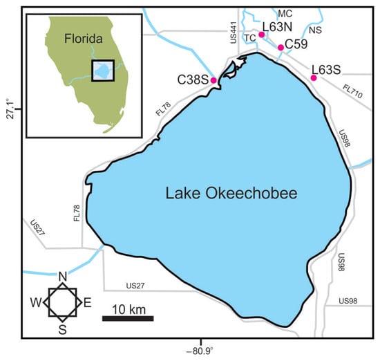
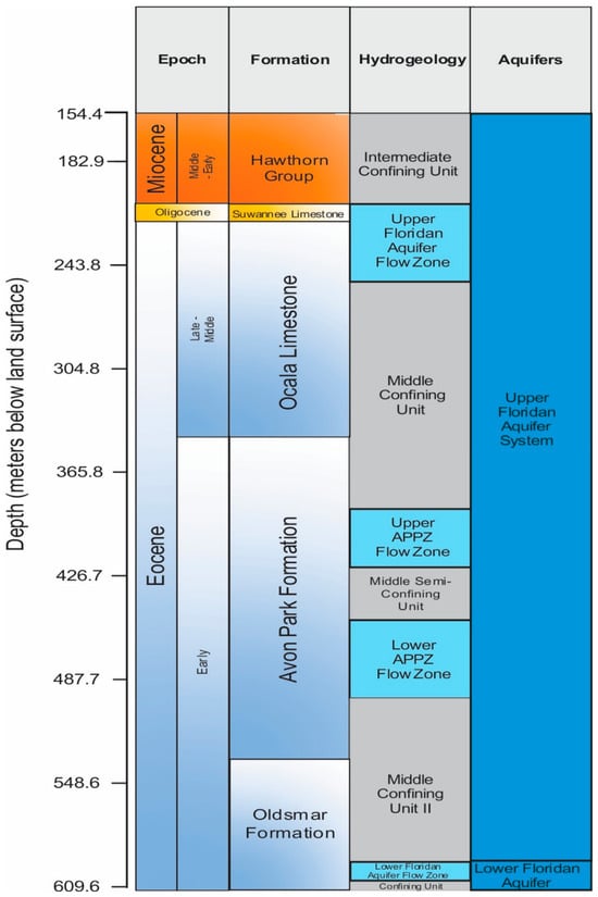
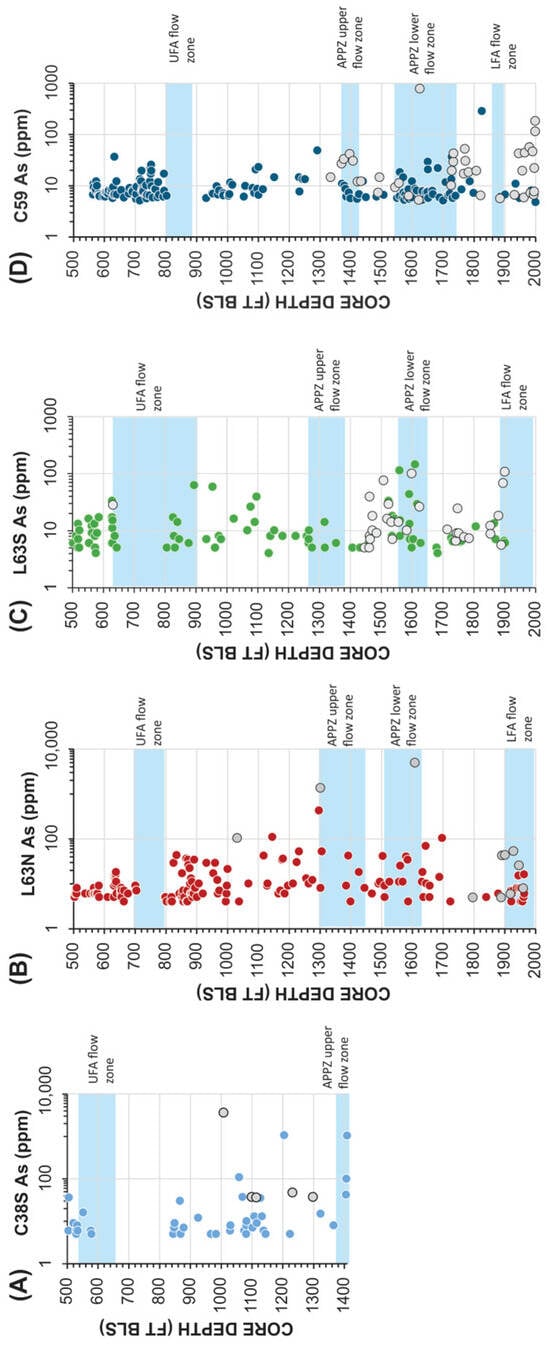
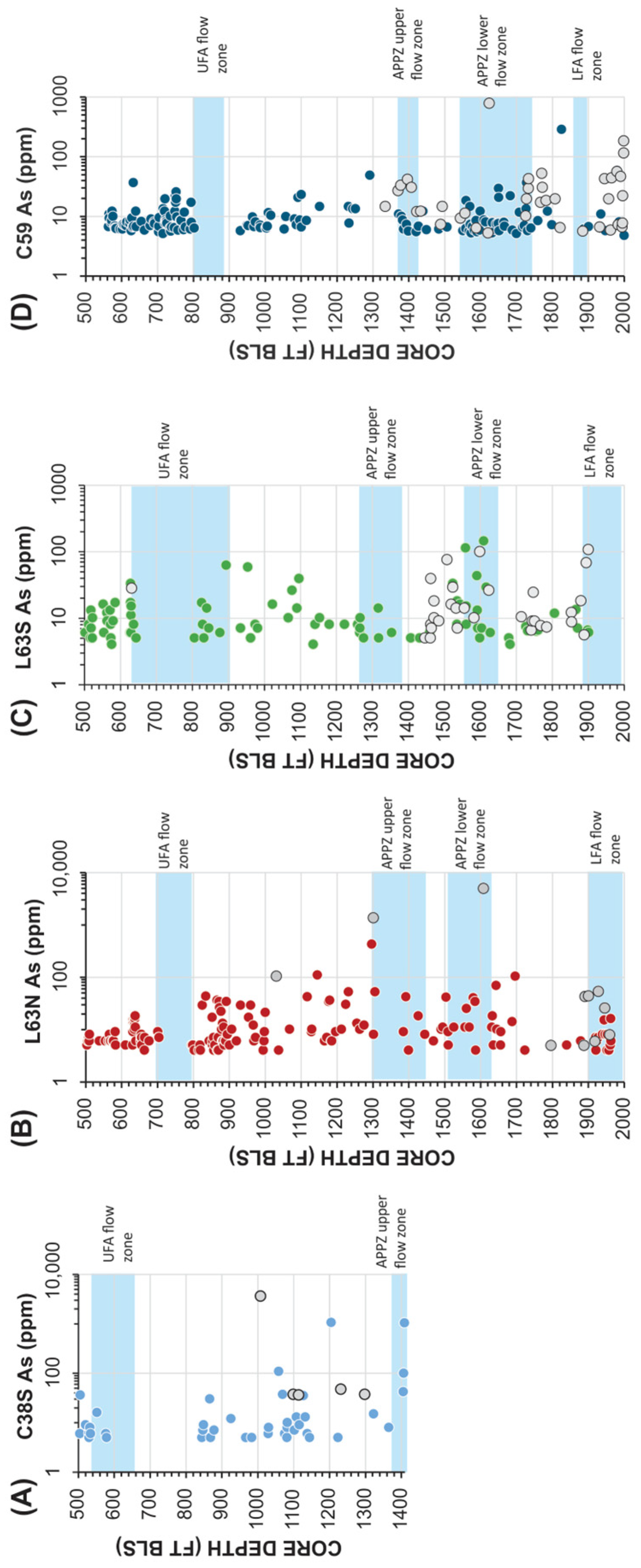
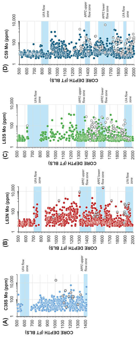
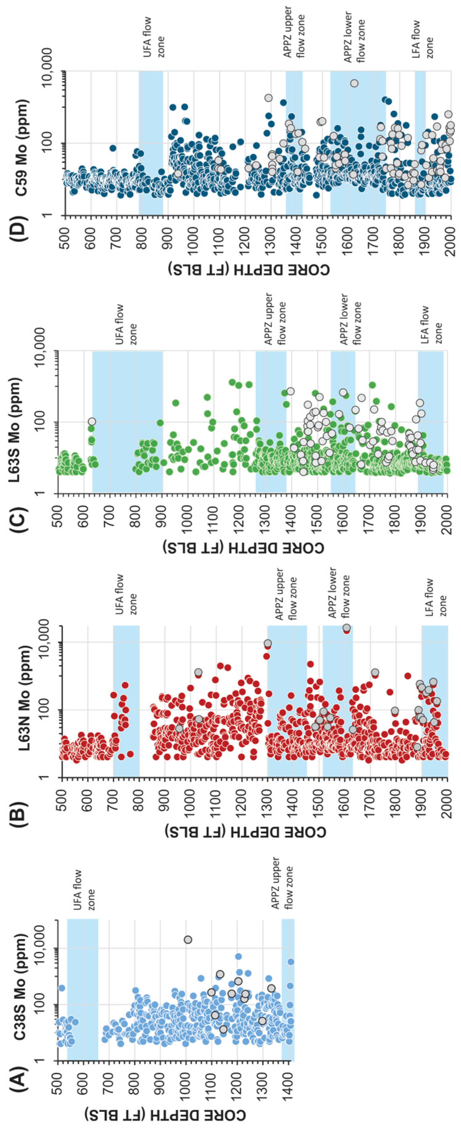
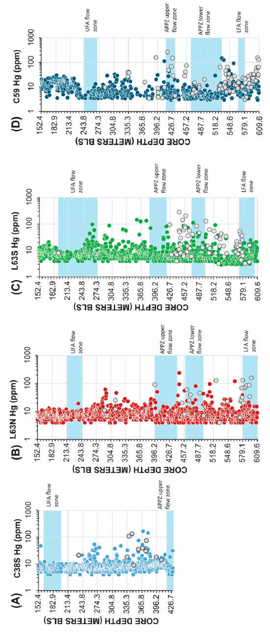
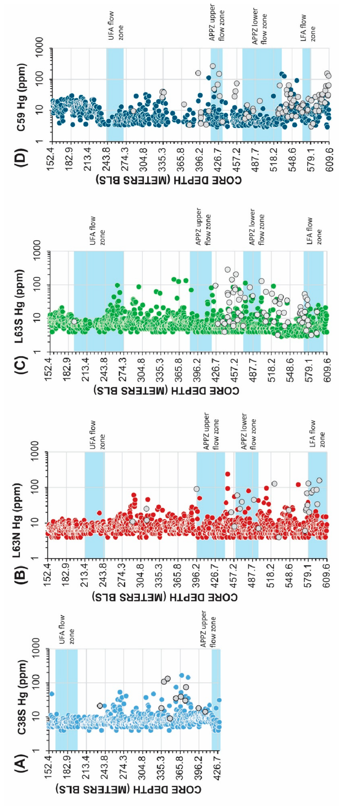

Disclaimer/Publisher’s Note: The statements, opinions and data contained in all publications are solely those of the individual author(s) and contributor(s) and not of MDPI and/or the editor(s). MDPI and/or the editor(s) disclaim responsibility for any injury to people or property resulting from any ideas, methods, instructions or products referred to in the content. |
© 2026 by the authors. Licensee MDPI, Basel, Switzerland. This article is an open access article distributed under the terms and conditions of the Creative Commons Attribution (CC BY) license.