Increasing Computational Efficiency of a River Ice Model to Help Investigate the Impact of Ice Booms on Ice Covers Formed in a Regulated River

Abstract

The formation and stability of river ice covers in regulated waterways are critical for uninterrupted hydro-electric operations. This study investigates the modelling of ice cover development in the Beauharnois Canal along the St. Lawrence River with the presence and absence of ice booms. Ice booms are deployed in this canal to promote the rapid formation of a stable ice cover during freezing events, minimizing disruptions to dam operations. Remote sensing data were used to assess the spatial extent and temporal evolution of an ice cover and to calibrate the river ice model RIVICE. The model was applied to simulate ice formation for the 2019–2020 ice season, first for the canal with a series of three ice booms and then rerun under a scenario without booms. Comparative analysis reveals that the presence of ice booms facilitates the development of a relatively thinner and more uniform ice cover. In contrast, the absence of booms leads to thicker ice accumulations and increased risk of ice jamming, which could impact water management and hydroelectric generation operations. Computational efficiencies of the RIVICE model were also sought. RIVICE was originally compiled with a Fortran 77 compiler, which restricted modern optimization techniques. Recompiling with NVFortran significantly improved performance through advanced instruction scheduling, cache management, and automatic loop analysis, even without explicit optimization flags. Enabling optimization further accelerated execution, albeit marginally, reducing redundant operations and memory traffic while preserving numerical integrity. Tests across varying ice cross-sectional spacings confirmed that NVFortran reduced runtimes by roughly an order of magnitude compared to the original model. A test GPU (Graphics Processing Unit) version was able to run the data interpolation routines on the GPU, but frequent data transfers between the CPU (Central Processing Unit) and GPU caused by shared memory blocks and fixed-size arrays made it slower than the original CPU version. Achieving efficient GPU execution would require substantial code restructuring to eliminate global states, adopt persistent data regions, and parallelize at higher level loops, or alternatively, rewriting in a GPU-friendly language to fully exploit modern architectures.

1. Introduction

The characteristics and extent of ice covers in regulated waterways can be influenced and controlled by structural interventions such as ice booms. These floating barriers are strategically placed to promote the formation of stable ice covers, reducing frazil transport and mitigating the risk of uncontrolled ice jamming near dams and other infrastructure. To evaluate the effectiveness of ice booms and understand their benefits in establishing a continuous cover without excessive thickening or severe ice jamming, river ice modelling is employed. Modelling allows practitioners to simulate freeze-up under current conditions with booms in place and compare these results to scenarios where booms are removed. Such analyses reveal that without booms, ice jams can become more pronounced [1,2], leading to significant backwater effects and posing operational threats to hydroelectric facilities. By integrating remote sensing observations with modelling, operators can better predict freeze-up behavior, optimize flow regulation, and maintain system reliability throughout the winter season.

An important objective of this technical note is to model the presence of ice booms during the formation of an ice cover during river freezing in the Beauharnois Canal using the river ice model RIVICE [3]. The modelling is to show the benefit of ice booms in establishing a stable ice cover by simulating a scenario without booms, showing how their absence can potentially lead to more extensive ice thickening, pronounced ice jamming, and increased backwater staging.

Another objective of the study is to explore means of increasing the efficiency of the RIVICE model, RIVICE is a legacy hydrodynamic river ice simulation program originally written in Fortran 77, an archaic language first published in 1977. As a Fortran 77 application, RIVICE relies heavily on fixed-form syntax and COMMON blocks (a Fortran feature that allows variables to be shared globally across multiple subroutines or functions by grouping them into a named memory block), all of which were standard practices in older Fortran codes but are problematic for contemporary high-performance computing. COMMON blocks provide “global” shared memory across subroutines hindering parallelization because modern GPU (Graphics Processing Unit which is a specialized processor designed to handle parallel computations, originally for rendering graphics but now widely used for accelerating scientific and data-intensive tasks) frameworks like OpenACC (Open Accelerators, a programming standard that uses compiler directives to enable parts of a program to run on accelerators like GPUs without requiring major code rewrites) require well-defined “local” memory scopes. The model also uses oversized static arrays declared in COMMON blocks, even though only a fraction is used. Such a design wastes memory and creates constraints when porting to GPUs, which require optimized data allocation. Attempts to copy COMMON-block variables into local scope or pass them as arguments revealed further structural weaknesses, including inconsistencies in type and dimensionality, leading to memory corruption and crashes.

Despite these limitations, RIVICE demonstrates the strengths of the Fortran language for numerical computation, particularly in solving the Saint-Venant equations and related hydraulic and thermodynamic formulations [3]. Modern compilers like NVFortran can optimize the legacy code without altering its structure, achieving increased speedup through loop unrolling, vectorization, and register optimization. Furthermore, proof-of-concept GPU acceleration using OpenACC confirmed that RIVICE can execute on modern architectures, although initial implementations suffered from excessive host–device data transfers and memory allocation issues caused by its legacy design.

2. Site Description

The Beauharnois Canal, a 25-km regulated section of the St. Lawrence Seaway, is characterized by relatively uniform geometry and controlled water levels maintained between approximately 44 and 46 metres above sea level (geodetic elevation). During winter, freeze-up processes in the canal are influenced by both thermal and hydraulic conditions, with frazil ice forming under sustained sub-zero air temperatures and gradually consolidating into an intact cover. High flow velocities near the dam may inhibit deposition and cause frazil submergence, delaying cover formation and increasing the risk of unstable ice movement upstream. To manage these dynamics and help maintain hydropower operations (along with a number of other river system considerations), flow is regulated during the ice season according to guidelines set by the International Joint Commission [4]. Ice booms are also strategically installed across the canal to initiate and stabilize an ice cover during freezing periods. These floating structures act as physical barriers that trap frazil ice and promote juxtaposition and consolidation upstream, reducing uncontrolled ice drift and mitigating the potential for ice jams near critical infrastructure. Ice booms are typically placed at key locations along the canal [5] to improve freeze-up stability and are designed with openings to maintain navigation, allowing some ice to bypass and accumulate downstream.

Understanding and predicting these freeze-up processes requires accurate spatial and temporal data, and remote sensing technologies can play a vital role in this effort. Space-borne sensors provide wide coverage of the canal and Lac Saint-François upstream of the canal, enabling the detection of large-scale ice patterns and freeze-up timing under varying thermal conditions. Airborne platforms offer higher-resolution imagery for monitoring localized features such as ice bridging at ice booms, open leads, and partial covers, while near-ground remote sensing delivers details on ice type, ice cover extent and degree of ice consolidation. Integrating these multi-scale observations with numerical models enhances the ability to simulate ice formation and progression, calibrate parameters such as ice thickness and roughness, and validate freeze-up scenarios under different flow and temperature regimes. This information is useful for managing the regulation of flow in the system, as accurate forecasts of ice cover development allow operators to adjust discharge and maintain ice stability, while minimizing the risk of ice jams and their resulting backwater effects. By combining remote sensing data with physical and numerical modelling, the Beauharnois Canal could potentially be managed more effectively during freeze-up, ensuring operational reliability and reducing the risk of ice-related issues.

3. Method

3.1. RIVICE Model Description

RIVICE is a one-dimensional implicit finite difference hydrodynamic river ice model that simulates major ice processes such as ice cover formation, frazil and border ice development, ice transport, juxtapositioning, shoving, ice jamming and hanging dam progression. The model provides a physically based framework for many applications such as forecasting ice jam flooding, ice jam flood hazard and risk assessments and climate-change scenarios. A control file provides the parameter and boundary-condition settings to steer ice deposition and ice cover erosion thresholds, leading edge stability, porosity and thickness of ice pans and accumulations in ice covers, in transit ice transport scaling, barrier effects (including ice jam lodgement locations and frictional shed factors), border ice growth methods, frazil ice production settings, hydraulic roughness formulations for both ice and bed, and meteorological forcing required for thermodynamic ice generation. The model requires upstream discharge of water and ice and downstream water level elevations as boundary conditions. Its outputs consist of longitudinal profile files and hydrograph files that report, for each time step and cross section, variables such as water surface elevation, depth, discharge, velocity, roughness, hydraulic radius, and ice cover thickness, enabling users to assess ice cover progression, ice jam formation, and resulting backwater staging along the modelled river reach.

3.2. Modelling Freeze-Up Ice Cover Formation

The modelling of freeze-up river ice processes in the Beauharnois Canal was conducted using the one-dimensional river ice model RIVICE, which simulates ice formation, progression, and stability under varying hydraulic and thermal conditions. A test case for the freeze-up of the Canal in the 2019–2020 ice season was investigated. The first step involved constructing a detailed geometric representation of the canal using surveyed cross-sections spaced approximately one kilometre apart and interpolated sections at finer intervals of 50 metres to capture localized hydraulic variations essential for ice dynamics. Bathymetric data from the Canadian Hydrographic Service [6] were adjusted to geodetic elevations using chart datums, and bank elevations were defined from Lidar data to ensure accurate computation of channel width and flow area at different stages.

The hydraulic component of the model was calibrated under open-water conditions before introducing ice processes. This calibration required generating rating tables that relate discharge to water surface elevation at each cross-section, using historical flow and water level data (Hydro Québec, personal communication) to establish initial conditions. Once the hydraulic setup was validated, ice processes were activated to simulate freeze-up. Frazil ice generation was modelled using two approaches: ice production based on air temperature and heat transfer coefficients, and volumetric ice input representing frazil ice inflow from upstream sources. The model accounts for key physical parameters such as ice thickness, porosity, bridging characteristics, and erosion and deposition thresholds, which govern the consolidation and stability of ice covers.

Surveyed cross-sections and ice cross-sections differ primarily in their purpose, spacing, and impact on model performance. Surveyed cross-sections are the original profiles obtained from field measurements or GIS data and are spaced relatively far apart, around one kilometer in this case. They provide the foundational geometry for the channel and are used to set up the hydraulic model and generate hydraulic rating curves. Because they represent actual surveyed data, they ensure that the model reflects real-world conditions, but their coarse spacing limits numerical solutions.

Ice cross-sections, on the other hand, are not directly surveyed but are interpolated between the surveyed cross-sections to create a finer spatial resolution of the model geometry. These interpolated sections are spaced much closer together, often at intervals of 5 m (for very steep river reaches) to 100 m (for very mildly sloped reaches) and are essential for simulating ice processes accurately. The finer spacing improves numerical stability and allows the model to capture gradual longitudinal changes in hydraulic and ice dynamics, such as jam formation and backwater effects. However, this increased resolution comes at a computational cost since smaller spacings, although yielding more stable and accurate simulations, require longer runtimes and more resource requirements (memory). Conversely, using coarser spacing speeds up the simulations but reduces stability and accuracy, sometimes leading to unrealistic results or model crashes.

To represent structural interventions, ice booms were incorporated into the model as lodgement points that promote juxtaposition and stabilize the ice cover. Scenarios were run with ice booms in place to replicate current operational practices and then repeated without booms to evaluate their influence on freeze-up dynamics. A basic scenario analysis focused on differences in ice extent, thickness, and backwater effects, highlighting the potential for severe ice jamming and elevated water levels when booms are absent. Remote sensing data, space-borne imagery for large-scale ice distribution, airborne observations for localized features, and near-ground surveys for more detailed ice characteristics, were integrated to calibrate the simulations, ensuring that modelled ice conditions aligned with observed freeze-up patterns. This combined approach provides a robust framework for future assessments of the effectiveness of ice booms.

3.3. Incorporating Remote Sensing in Model Calibration

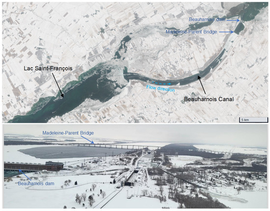
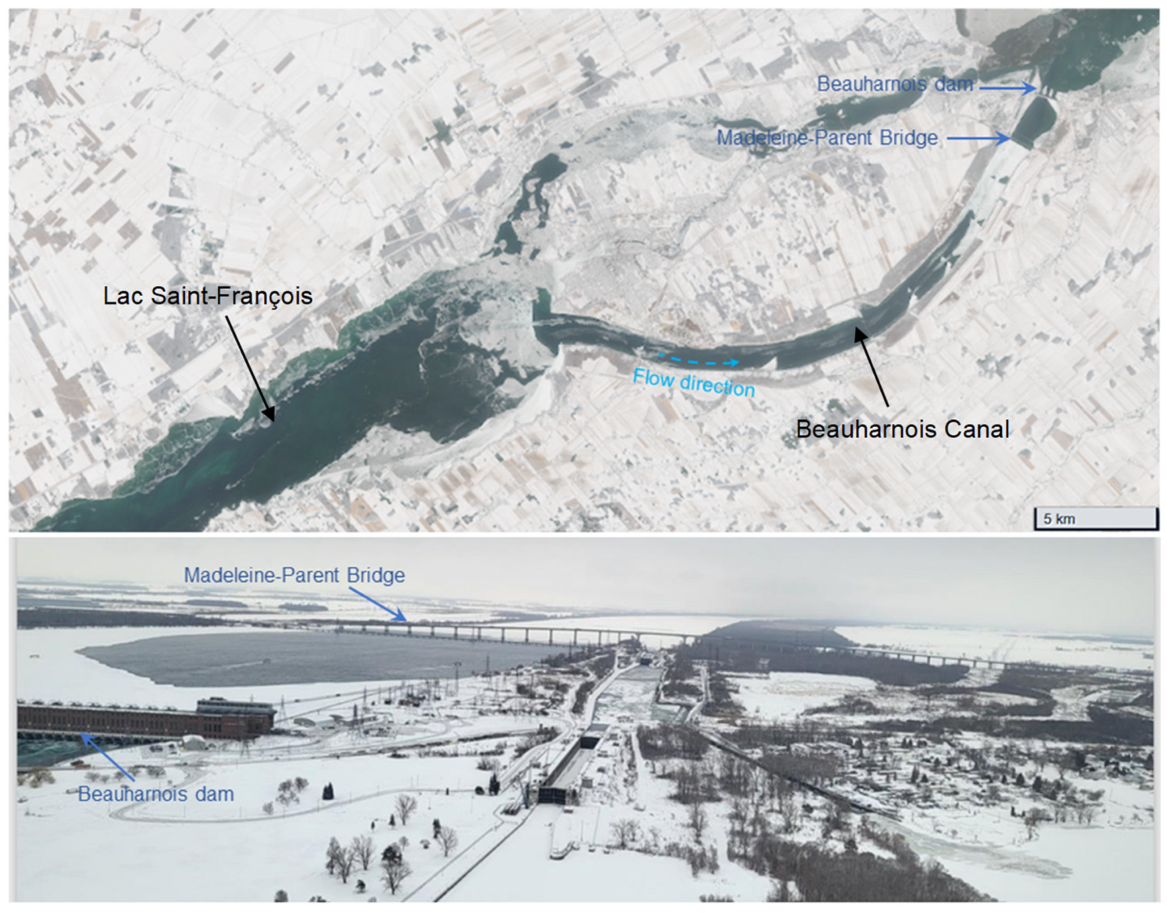
Remote sensing data were essential for calibrating the river ice model RIVICE because they provided spatial and temporal observations of ice conditions that could not be captured through ground measurements alone. Space-borne imagery (see top panel of Figure 1 for an example) offer synoptic views of the Beauharnois Canal and its upstream reaches, allowing identification of freeze-up timing, ice extent, and the progression of an ice cover under varying meteorological and hydraulic conditions. For example, images and an assessment of the seasonal progression of ice cover in the canal over 10 years, see Sudom et al. [7]. In the images for winter season 2021–2022, it was determined that much of the frazil ice does not stem from the canal itself but from the large surface area of Lac Saint-François upstream (west) of the canal. Airborne surveys (see bottom panel of Figure 1 for an example) can complement this by delivering high-resolution observations of localized features such as bridging at ice booms, open leads, and partial ice covers, which are critical for validating the model’s representation of ice formation and consolidation.

Figure 1. Sentinel-2 image taken 22 December 2021 (top panel); aerial photograph taken 10 March 2025 (bottom panel) of the Beauharnois Canal (from Canadian Coast Guard: https://e-navigation.canada.ca/topics/ice/daily-briefings (accessed on 11 January 2026).

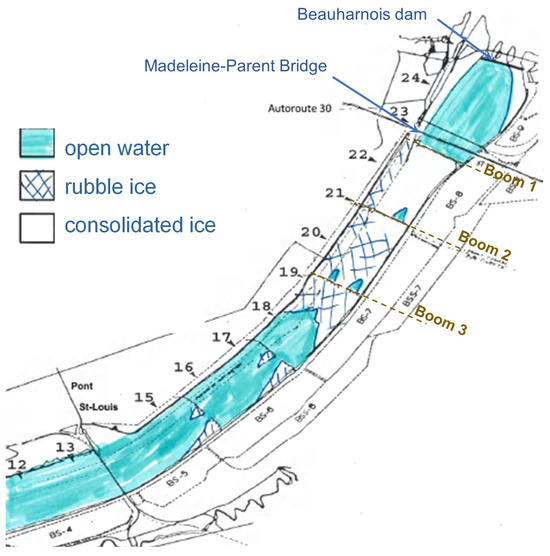
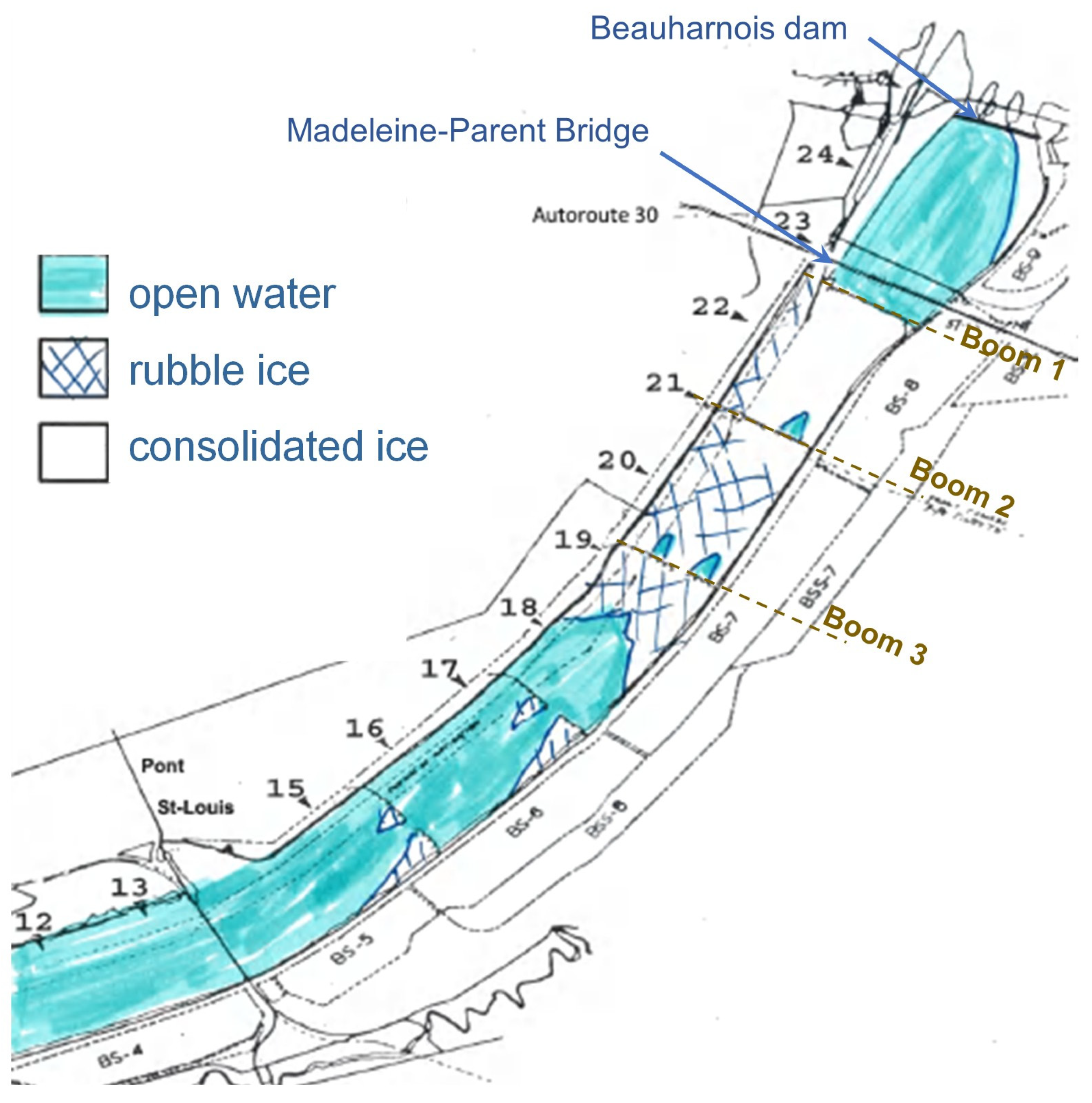
Near-ground remote sensing (human observations from bridges and canal banks) provided details (see Figure 2) of ice type and degree of consolidation, enabling fine-scale model calibration of ice cover extent and lodgement characteristics.

Figure 2. Example sketch of ice types from near-ground observations along the Beauharnois Canal for one date in the 2019–2020 ice season. Sketch courtesy of Hydro Quebec, with annotations (dam, bridge and ice boom locations) by authors.

These multi-scale datasets were integrated into the modelling workflow to adjust input parameters and validate simulation outputs. Observed ice cover extent and type from remote sensing were compared against modelled profiles to ensure that the simulated freeze-up dynamics reflect real-world conditions. For example, satellite imagery confirmed the timing and spatial distribution of intact ice covers, while human observations helped refine the calibration of lodgement points at ice booms by verifying where ice accumulation occurred and how quickly it progressed. By combining these observations with hydraulic and meteorological data, the model was tuned to reproduce observed freeze-up behavior accurately, thereby improving confidence in scenario testing, in particular simulations without ice booms. This integration of remote sensing data was critical for understanding the effects of ice booms and for ensuring that the model could reliably predict ice cover formation under different regulatory and environmental conditions.

3.4. Calibration Procedure

The modelling was calibrated by prescribing an upstream ice volume input that was allowed to accumulate naturally along the model domain, first forming a lodgement at the most downstream location corresponding to the first ice boom, where the inflowing ice began to juxtaposition and consolidate into an ice cover. As more ice entered the system and the thickness and extent of the cover increased, a second lodgement point representing the second ice boom was inserted, allowing the upstream portion of the cover to continue accumulating until the progressing ice reached the third and most upstream boom, at which point its lodgement allowed the extension of the ice cover further upstream in accordance with the observed freeze up sequence. The spatial extents of each successively formed ice cover were compared against satellite imagery, airborne observations, and near ground survey records to ensure that the simulated freeze up patterns matched the real-world ice cover and lodgement characteristics. Model performance was quantified by comparing simulated ice cover lengths, lodgement positions, and freeze up timing with remotely sensed extents and control observations, ensuring that the numerical results reproduced the documented progression of the ice cover under the influence of the three booms.

3.5. Analytical Solution for Ice Production

Frazil ice production in the simulations was first generated by modelling the transfer of heat from the canal water into the freezing air, but this approach quickly demonstrated that the surface area of the Beauharnois Canal is too small to produce the large volume of frazil ice required to form a continuous ice cover at the locations of the booms for the meteorological conditions of the simulation timeframe. Consequently, ice production was instead mimicked by introducing an upstream inflow of frazil ice representing ice formed on Lac Saint-François, whose much greater surface area provides a larger open-water region for supercooling and frazil ice generation. Satellite imagery confirmed that ice formation occurred on the lake upstream of the canal, validating the conceptual basis for applying an upstream frazil ice inflow rather than relying solely on in-canal production.

To further justify this modification, a simple analytical estimate was carried out to approximate the potential frazil ice volume generated over the lake compared to that from the canal’s smaller water surface. Using the analytical expression for ice production [8]:

$$V_i={\int }_{t_0}^t{\displaystyle \frac{H_{wi}A(T_w-T_a)\hspace{0.17em}dt}{{\rho }_i\lambda }}$$

applying its discrete form,

$$V_i={\displaystyle \frac{H_{wi}A(T_w-T_a)∆t}{{\rho }_i\lambda }}$$

and simplifying the expression by setting $T_w=0$ °C yields

$$V_i={\displaystyle \frac{-T_a\hspace{0.17em}{H}_{wi}\hspace{0.17em}A\hspace{0.17em}∆t}{{\rho }_i\lambda }}$$

where $T_a$ is the freezing air temperature (ranging between −20.7 °C and −11.9 °C from 20 to 21 December 2019), $H_{wi}$ is the heat transfer coefficient (18–25 W/m²/°C), $A$ is the open-water supercooling area (equal to supercooling length times average width), ${\rho }_i=920\hspace{0.17em}{\mathrm{kg}/\mathrm{m}}^3$ is the ice density, $\lambda =\mathrm{334,944}\hspace{0.17em}\mathrm{J}/\mathrm{kg}$ is the heat of fusion, and $∆t$ is the time over which freezing occurs (24 h).

The analytical ice production equation was incorporated into a Monte-Carlo framework so that it could be solved hundreds of times using randomly sampled values of the variables, each drawn from prescribed minimum-to-maximum ranges rather than fixed values. This approach ensured that, instead of producing a single deterministic estimate of the total frazil ice volume generated, the model yielded full probability distributions of possible ice production outcomes, reflecting the inherent uncertainty in parameters such as air temperature, heat transfer coefficient, open-water area, and freezing duration. Following the methodology outlined by Lindenschmidt [9], the Monte-Carlo procedure was implemented in a spreadsheet environment (provided in the Supplementary Materials), allowing the last analytical expression above to be repeatedly evaluated under randomized input conditions. As a result, the exercise produced distributions rather than point estimates, enabling an assessment of the likelihood of different ice production volumes and providing insight into the calculations uncertainty.

By calibrating the ranges of all variables involved in the analytical estimation of ice volume, the length of the ice cover L_i formed by the three-boom configuration was determined by dividing the calculated ice volume V_i by the product of the representative ice thickness h_i and the width of the formed ice cover w_i:

$$L_i={\displaystyle \frac{V_i}{h_i{ w}_i}}$$

with the variable ranges fine-tuned until L_i matched the actual ice cover length determined from remote-sensing data. The ice thicknesses were extracted from the RIVICE simulations, which followed a gamma distribution. The widths were drawn from a uniform distribution ranging between the minimum and maximum width of the canal.

3.6. Improving Computational Efficiency

RIVICE was originally compiled using a Fortran 77 compiler, which limits the use of modern optimization techniques. Recompiling the code with NVFortran immediately improves performance because the compiler provides more efficient instruction scheduling, enhanced cache management, and better exploitation of CPU resources. Even without explicit optimization flags, NVFortran reduces runtime due to its ability to automatically analyze loop structures and generate more effective machine code for array-based numerical operations.

When optimization is enabled, NVFortran further accelerates RIVICE by applying techniques such as loop unrolling, vectorization (SIMD = single instruction, multiple data), loop-invariant code motion, and subroutine inlining. These transformations reduce redundant operations, increase instruction-level parallelism, and minimize memory traffic, which are critical for models like RIVICE that depend on deeply nested loops and large array computations. As a result, the compiler achieves substantially faster execution while preserving the numerical behaviour of the legacy Fortran 77 implementation.

To enhance computation speeds even further, an attempt was made to dock RIVICE to a GPU using a directive-based approach (to avoid extensive re-writes of the original code) with OpenACC inside the NVFortran compiler to allow selected loops to be offloaded to the GPU while keeping most of the legacy Fortran 77 structure intact. First, computationally intensive routines were identified in RIVICE, such as the inner loop of the PARAM(K) subroutine and the outer loop in SOLVE, as these sections repeatedly perform independent calculations across cross-sections. To make these loops GPU-compatible, all data dependencies were made explicit by removing COMMON blocks and passing arrays as arguments, since OpenACC requires clear data scope for device memory allocation. Next, data movement directives were introduced to copy necessary arrays from host memory to the GPU using COPYIN and CREATE clauses, and to return updated values with COPY after kernel execution. Inside the PARAM(K) loop, OpenACC directives are applied to distribute iterations across GPU thread blocks and threads. Commands were implemented to retain large arrays on the GPU for the entire computation instead of repeatedly transferring them between CPU and GPU.

4. Results and Discussion

4.1. River Ice Simulations

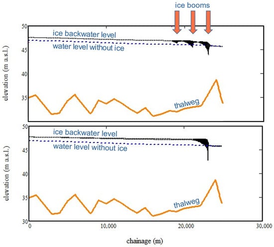
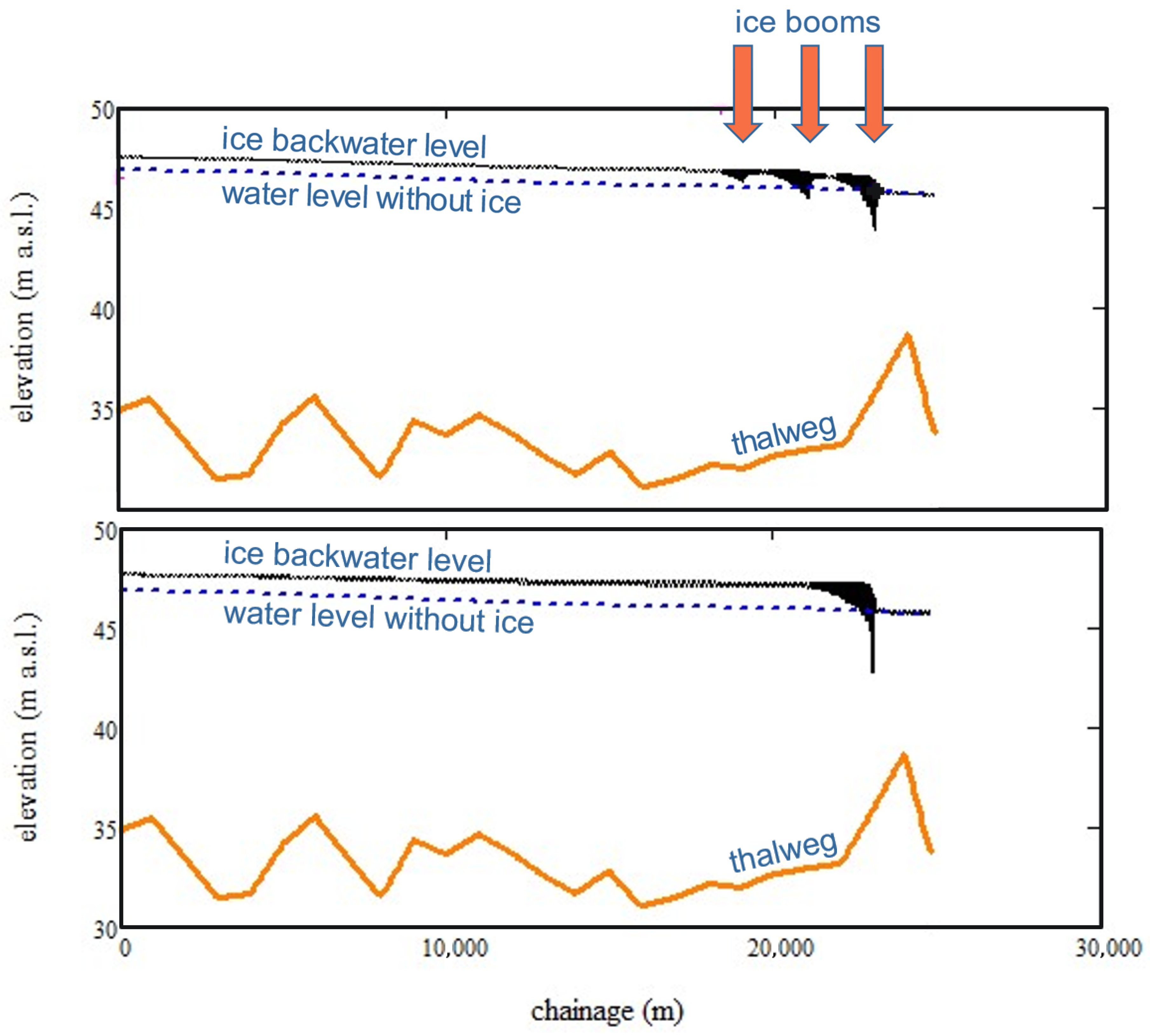
As detailed in Abdelnour et al. [5], seven ice booms are typically deployed in the Beauharnois Canal. For the purposes of the present study, only three of these were modelled. Figure 2 identifies the locations of those three booms (Booms 1, 2, 3). Modelling of an ice cover with ice booms showed that booms significantly influence ice accumulation and backwater effects by distributing the ice cover further upstream with a thinner cover, thereby spreading the ice more uniformly and thinner along the channel. Figure 3 shows simulated longitudinal profiles of the ice cover, with ice booms (top panel) and without booms (bottom panel). The ice cover with backwater level profile is shown in black and the dashed blue line indicates the water surface profile without ice. Together, the two profiles provide an indication of the amount of backwater caused by the ice cover. At km 20, the backwater staging is 60 cm higher for the no-boom scenario than with the simulation with ice booms.

Figure 3. Simulated ice covers with three ice booms (top panel) and without booms (bottom panel).

Remote sensing data were critical for calibration. Satellite imagery and near-ground surveys provided accurate observations of ice cover extent, lodgement locations, and freeze-up timing, ensuring that the simulated ice cover matched actual conditions. Importantly, in addition to the modelling, remote sensing imagery verified that most of the ice forming the canal’s cover does not originate within the canal itself. Instead, the ice comes from the much larger surface area of Lac Saint-François further upstream in the St. Lawrence River. An attempt was made to model the ice cover using only frazil ice generated within the model domain, i.e., only the extent of the canal. Not enough ice could be generated in the simulation to form the vast volume of ice necessary for the formation of the ice cover. This suggests that the canal’s limited surface area cannot generate enough frazil ice to form a continuous cover. Field observations would be required to validate this finding. Hence, the modelling was extended to augment the ice volume by inserting ice in the upstream boundary (canal inlet), representing ice originating from Lac Saint-François. This insight of complementing the volume of ice with an additional source from upstream of the canal was essential for defining correctly ice inflow to the model. Without remote sensing, calibration would rely solely on assumptions, limiting accuracy and confidence in the results. By integrating these observations, the model achieved a higher degree of reliability, supporting scenario analysis of structural interventions such as ice booms.

Comparing the simulations with and without ice booms also indicates that booms help to distribute the ice in a thinner and more uniform manner along a longer stretch of the canal, preventing excessive ice cover thickening due to ice jamming and less staging of the backwater effect.

4.2. Analytical Solution of Ice Production Within Monte-Carlo Framework

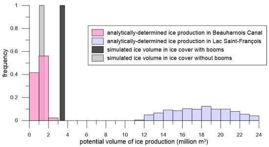
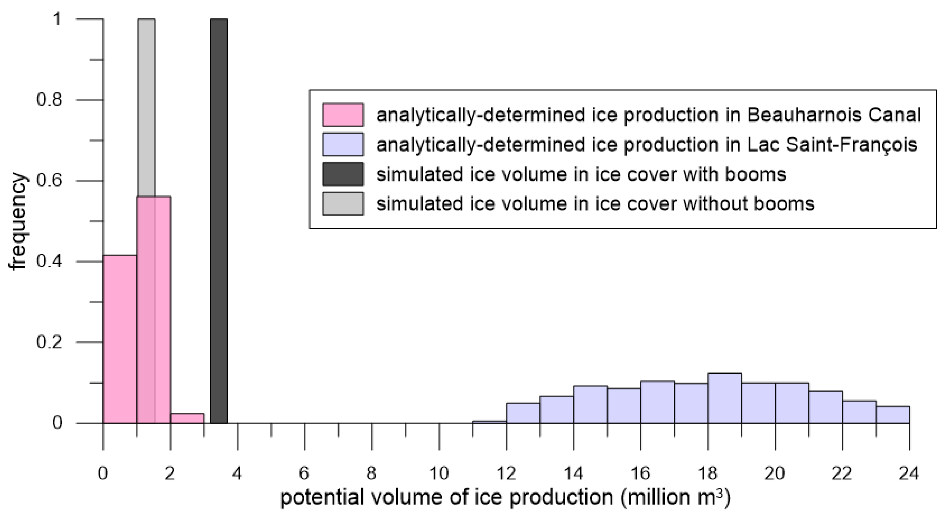
Referring to Figure 4, the analytical exercise for calculating ice production shows clearly that, under the meteorological conditions of the period being modelled, the Beauharnois Canal lacks the surface area to produce enough frazil ice to form and sustain a stable ice cover at the boom locations. However, the surface area of Lac Saint-François is sufficiently large to produce the ice volume required for an ice cover to form in the canal. Using the Monte-Carlo implementation of the analytical ice production equation, the simulations showed that the canal could generate only an average of approximately 1 million m³ of frazil ice, whereas the lake could produce, on average, roughly eight million m³ over the same time frame. These results reinforce the conclusion that the lake can be a dominant source of ice input to the canal.

Figure 4. Analytically derived histograms of the potential ice that could be produced in the Beauharnois Canal and Lac Saint-Francois; volume of ice simulated in the ice cover, with and without booms.

For the same total inflow of ice into the RIVICE model domain (3.9 million m³) the simulations showed a pronounced difference in how much ice ultimately accumulated in the stable ice cover, depending on whether ice booms were present. Again, referring to Figure 4, in the scenario with three ice booms, approximately 3.7 million m³ of ice (0.2 million m³ less than the 3.9 million m³ due to ice in-transit between the upstream boundary and the ice cover front) became incorporated into the ice cover, indicating that nearly all of the inflowing ice was retained upstream through early deposition and controlled lodgement at the boom locations. In contrast, the no-boom scenario accumulated only 1.5 million m³ of ice in the cover, revealing that a substantial portion of the inflowing ice was eroded from the underside of the forming cover, transported further downstream, and unable to consolidate. This result reflects the much less stable freeze-up conditions without booms, where the ice cover thickens abruptly, could lead to higher underside shear and more frequent erosion events.

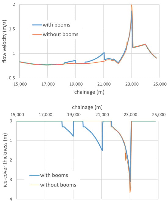
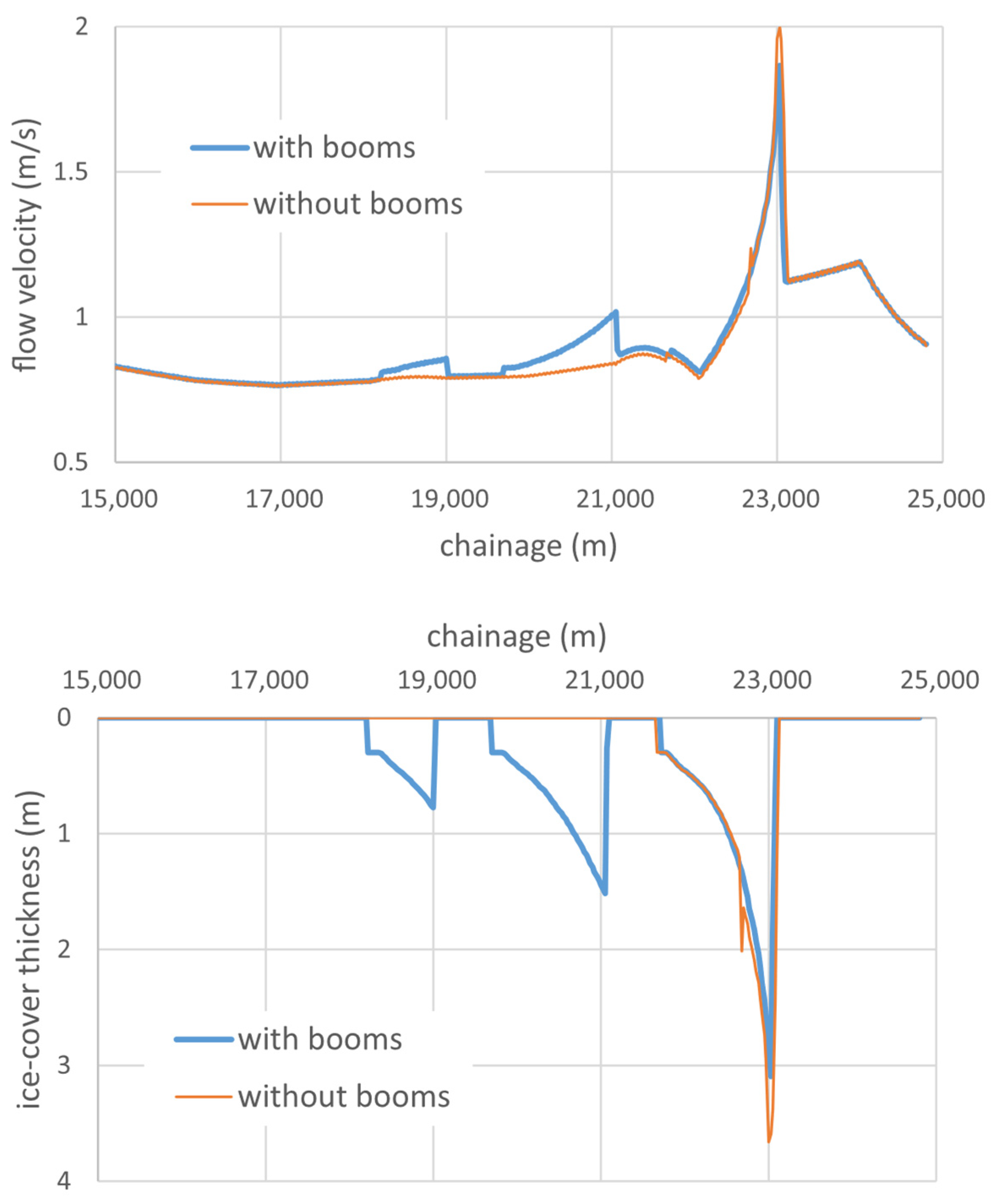
Figure 5 emphasizes the results of there being considerably more erosion in the no-boom scenario than in the boom scenario, as demonstrated by both the flow-velocity and ice-thickness profiles. In the boom scenario, flow velocities reach a maximum of only about 1.87 m/s near the downstream-most boom, remaining below the 2 m/s threshold at which the underside erosion threshold was set in the model. In contrast, the no-boom scenario exhibits flow velocities that exceed 2 m/s, activating sustained erosion and preventing stable consolidation of the forming ice cover. This difference in hydraulic forcing explains why the area under the ice-thickness profile is much larger for the boom scenario in which substantially less ice is eroded. This allows more of the inflowing ice to accumulate and form a more continuous cover compared to the no-boom case.

Figure 5. Longitudinal profiles of flow velocities (top panel) and ice cover thicknesses (bottom panel) along the Beauharnois Canal for the with-boom and no-boom scenarios.

Because the eroded ice in the no-boom simulations travels further downstream before consolidating, it carries an operational risk due to the potential of drifting ice reaching the dam forebay, where it could interfere with hydropower generation or trigger undesirable ice accumulations to jeopardize flow regulation. In contrast, when ice booms are installed, deposition initiates earlier and at multiple controlled lodgement points, which stabilizes the leading edge of the cover, reduces the frequency and severity of underside erosion, and prevents large volumes of ice from being transported toward the dam. This stabilization effect smooths the upstream progression of the ice cover, reduces intense thickening events, and ensures that most of the inflowing ice becomes incorporated into a continuous and uniform cover well before reaching the hydropower facilities.

The freezing event simulated for this case study was relatively short in duration, hence only three ice booms of the seven were required to be incorporated into the modelling. However, even with three booms, the dominant controls on ice cover formation could be evaluated. These three booms exert the greatest hydraulic and ice-retention influence during the early stages of freeze-up, when the formation and stabilization of the ice cover are most sensitive to structural controls. The downstream booms are positioned closest to the dam and serve as the first and most critical barriers for initiating stable lodgement, trapping frazil ice, and preventing uncontrolled ice transport toward the hydropower facility. Their role therefore dominates the system’s response relative to the more upstream booms, which influence a region where the ice cover is typically already consolidated by the time it reaches them.

4.3. Enhanced Computational Efficiency Using NVFortran Compiler

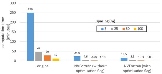
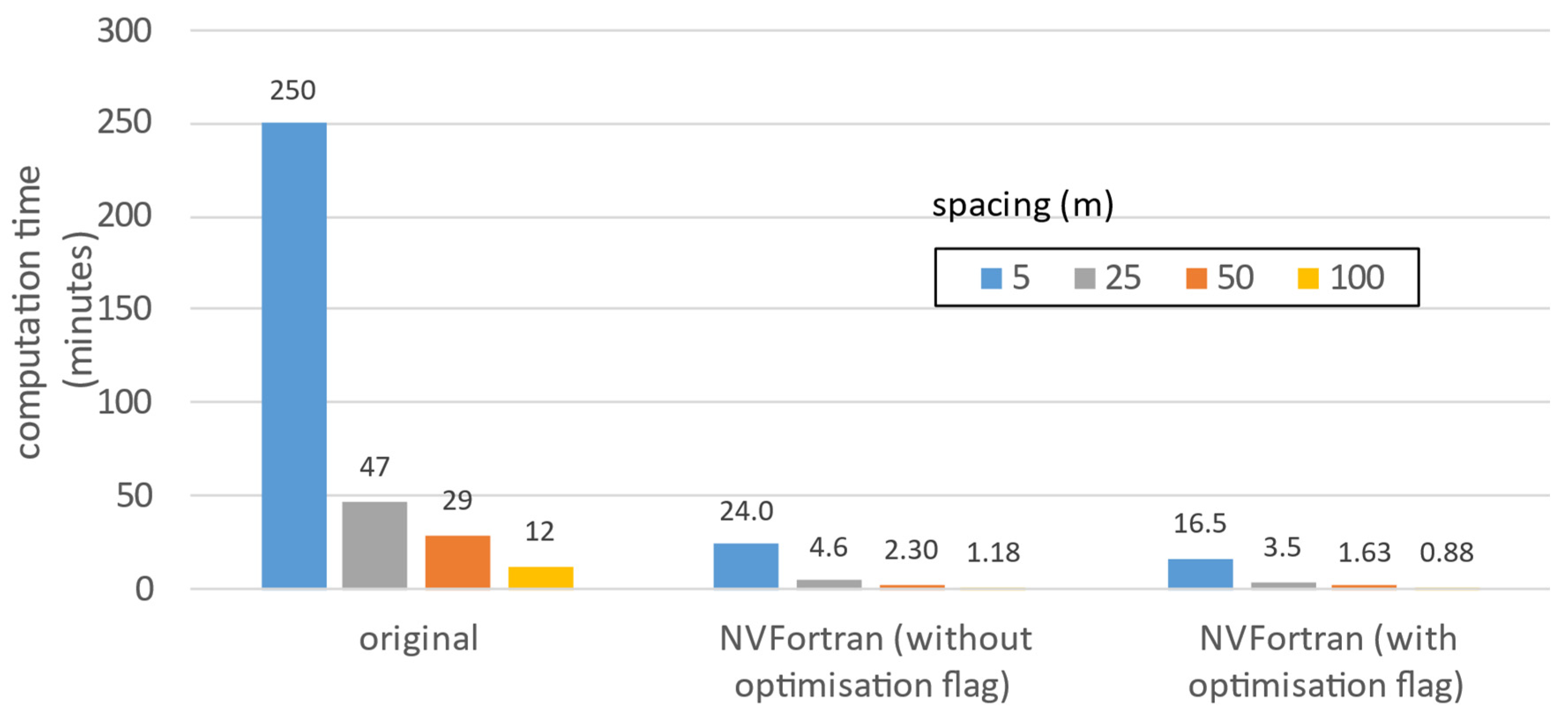
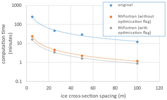
The model was tested using different spacings between ice cross-sections, 5, 25, 50, and 100 m, to evaluate the impact of geometric resolution on computational performance. These runs were first executed with the original Fortran 77 compiler and then with the NVFortran compiler, the latter in both non-optimized and optimized modes. As expected, simulations with the finest spacing of 5 m required the longest computational times because the increased number of cross-sections significantly raises the numerical load (see Figure 6). Conversely, the coarsest spacing of 100 m produced the fastest runtimes, reflecting the reduced computational demand.

Figure 6. Computational times of the Beauharnois Canal model stemming from different compilations and ice cross-sectional spacings.

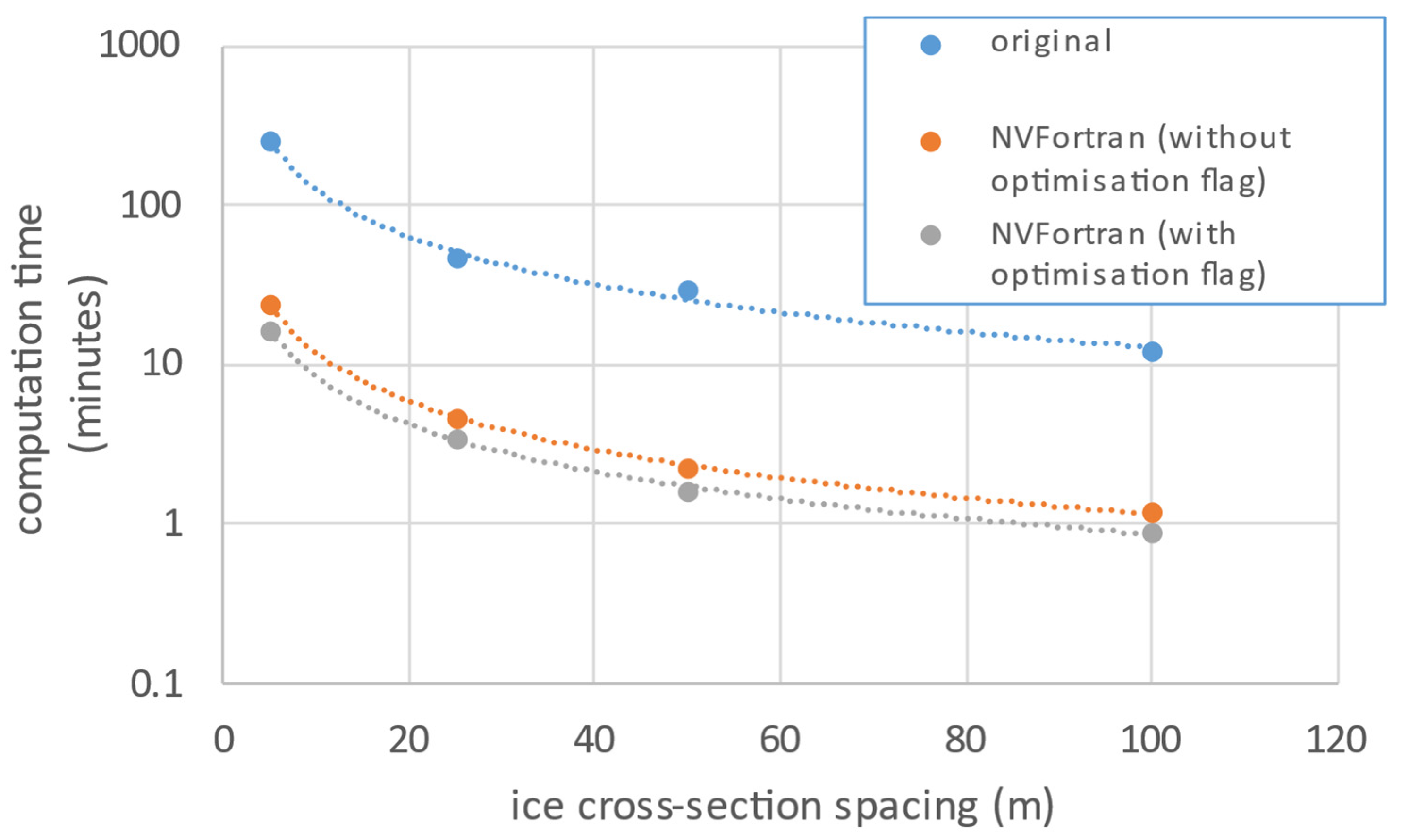
When comparing compilers, the original Fortran 77 implementation was markedly slower, highlighting the limitations of legacy toolchains for modern high-performance computing. Switching to NVFortran resulted in a dramatic improvement in execution speed, reducing runtimes by approximately an order of magnitude (Figure 7) thanks to its advanced optimization implementations. Applying the compiler’s optimization level (e.g., –O₂) provided only a fractional additional gain beyond the baseline NVFortran performance. This may be due to RIVICE’s archaic code structure which limits optimization potential. The legacy Fortran 77 code relies heavily on COMMON blocks and implicit typing, which restrict the compiler’s ability to fully exploit advanced optimizations.

Figure 7. Reorganizing the data from the previous figure to emphasise the order of magnitude differences in computational times between compilation types and ice-cross-sectional spacings in the model geometry.

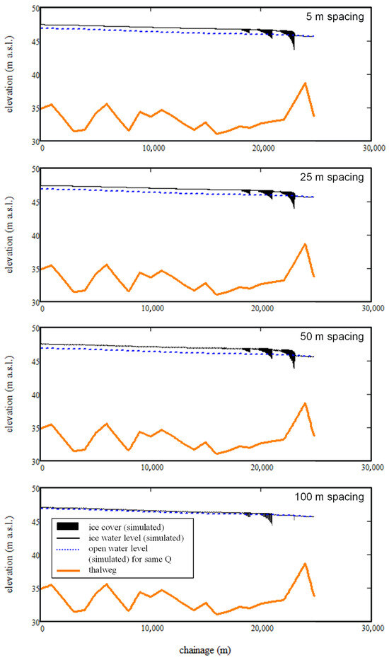
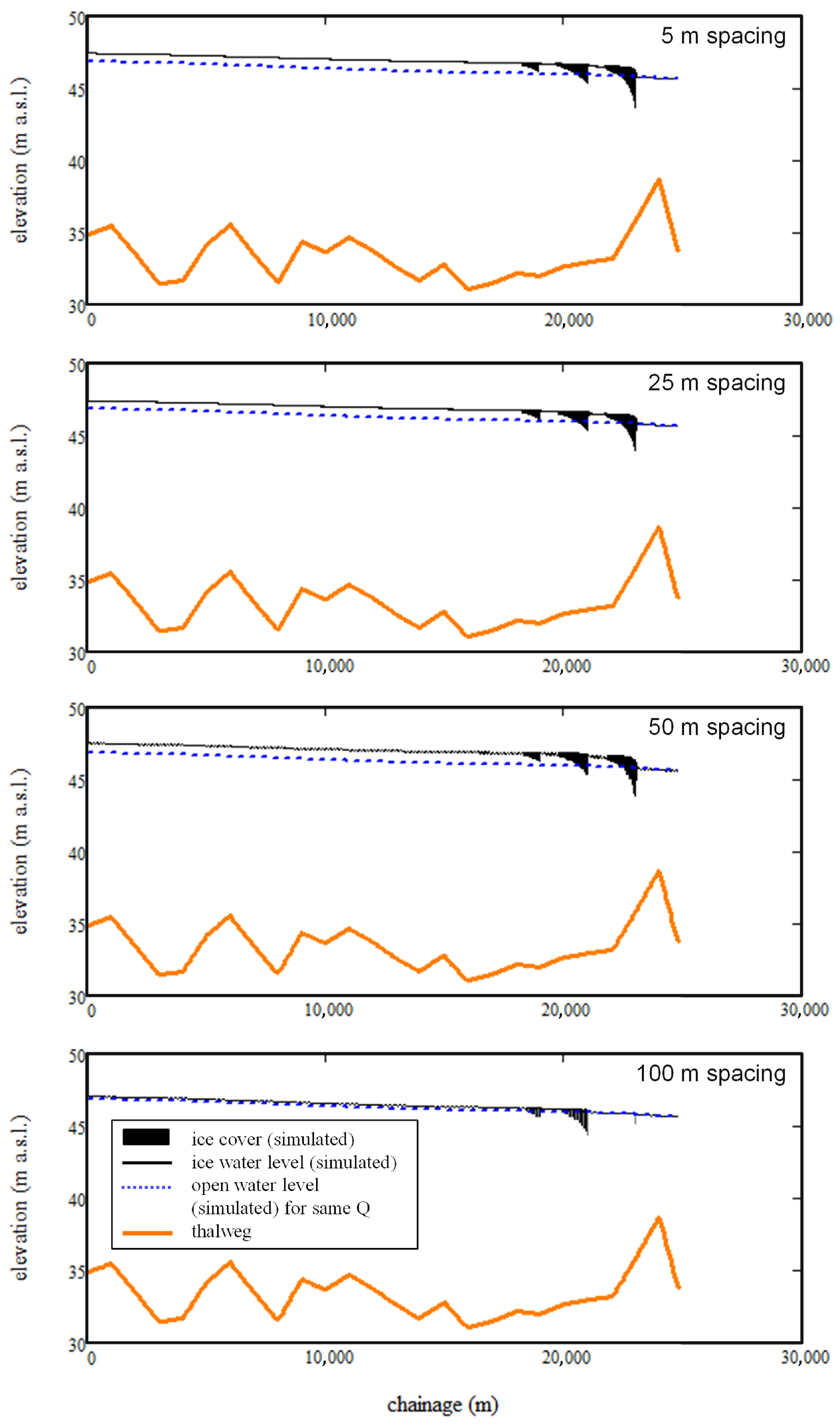
A comparison of the simulated backwater profiles for the 5-, 25-, 50- and 100-m spacings of the ice cross-sections is provided in Figure 8. The model simulations are stable for the first three spacing intervals; however, with the 100 m spacing, the resolution becomes too coarse for all the ice to accumulate in the downstream ice boom causing a drop in the backwater staging due to numerical instabilities. This demonstrates that high spatial resolution is essential for maintaining the numerical stability and accuracy of the simulations, emphasizing the need to adopt high-performance computing techniques.

Figure 8. Simulated profiles for the, from top to bottom, 5-, 25-, 50- and 100-m ice cross-sectional spacing model geometries.

4.4. RIVICE-GPU Docking

The GPU implementation of RIVICE confirmed that OpenACC directives correctly offloaded the subroutines of the PARAM(K) function to the device. The internal computations were mapped to gangs and vectors as expected, and diagnostic logs verified proper arithmetic operations on device memory. However, the performance was constrained by frequent host–device data transfers. Because the model relies on COMMON blocks and oversized static arrays, the compiler was forced to repeatedly copy large memory regions between the CPU and GPU. These transfers dominated the runtime and eliminated the potential benefits of parallel execution, resulting in slower performance than the CPU baseline. The experiment demonstrated that a legacy Fortran 77 model can run on modern GPU hardware, providing a foundation for future improvements such as reducing global state, restructuring arrays, and creating persistent data regions to minimize transfer costs.

For RIVICE-GPU docking to work most efficiently, the RIVICE code would need significant restructuring to eliminate COMMON blocks, make all data dependencies explicit, and use persistent OpenACC data regions so arrays remain on the GPU across multiple solver stages. Loops should be parallelized at a higher level, such as the outer PARAM and SOLVE loops, to increase computational intensity and reduce host-device transfers. Oversized arrays should be resized or replaced with dynamic allocation to facilitate GPU implementations, and subroutines should be refactored to pass arguments explicitly rather than relying on global states.

A feasible option would be to rewrite the RIVICE code in a different language that is better suited for GPU programming. The most appropriate choice would be either C or C++, as these languages integrate seamlessly with parallel computing platforms allowing developers to use GPUs for general purpose computing. This would allow full exploitation of GPU architecture and enable more advanced optimization strategies than those possible with legacy Fortran.

In the current implementation, host–device data transfers scale directly with domain size. Under the existing COMMON-block architecture, this linear increase in data movement outweighs the compute-bound portions of the solver, causing data transfer overhead to dominate runtime and limiting the effectiveness of GPU acceleration. Not until the code can be refactored (improving coding structure, data layout and program logic) to minimize transfers, create persistent device resident data regions (keeping memory allocations on the GPU intact), and pass only the minimal arrays required for each kernel will performance gains be noticeable.

Similar improvements in computational efficiency could be achieved for other river ice models and hydraulic solvers if an architecture-aware redesign is adopted, going beyond compiler-level optimization. From a GPU perspective, using a structure-of-arrays approach and fusing kernels for sequential physical processes would improve memory access and computational intensity. For models with spatially varying resolution, hybrid CPU–GPU strategies could be employed, with high-level control on the CPU while computationally intensive hydraulic and ice-process solvers are offloaded to the GPU. Additional performance gains could be achieved through advanced parallelization strategies, such as multi-GPU domain decomposition for scenario-based simulations. In the longer term, rewriting key solver components in GPU-native frameworks (e.g., CUDA, C++) would allow these models to fully leverage modern accelerators, improving scalability and performance while maintaining the same physical equations.

5. Conclusions

The modelling study demonstrated that ice booms can significantly influence ice cover formation and hydraulic conditions in the canal, creating localized ice retention and reduced backwater effects compared to scenarios without structural intervention. Accurate simulations required detailed calibration of parameters such as ice inflow, roughness coefficients, and lodgement characteristics, and this process highlighted the importance of incorporating remote sensing data into the modelling workflow. Satellite imagery, aerial photographs and near-ground surveys (human observations from bridges and canal banks) provide essential information on the spatial extent of ice cover and lodgement locations, enabling the model to replicate observed freeze-up dynamics. Remote sensing imagery also suggested that the ice forming the canal’s cover originates primarily from Lac Saint-François, as the canal’s limited surface area might not generate sufficient frazil ice to result in a continuous cover. This was substantiated with an unsuccessful attempt to generate enough frazil ice through the heat transfer from the canal water to the atmosphere alone. This insight was fundamental for including inflowing ice to the upstream boundary to ensure a realistic ice supply in the simulations.

The differences in simulated ice cover thicknesses and extent may be driven primarily by hydraulics. The stabilizing effects of ice booms, while ice supply acts as a necessary component, is due to the lessening of the under-ice cover erosion induced by the flow. Future work could entail numerical experiments in which flow would be incrementally increased to determine at what threshold flow the ice cover “washes out” for different ice supply conditions. This would help determine to what extent hydraulics, compared to ice supply, influences ice cover thickness and stability.

This work demonstrated the importance of integrating remote sensing data in the calibration and validation of a numerical river ice model. The hybrid approach of combining numerical simulations with remotely sensed observations could support planning and risk assessment for dam and hydropower generation operations. Future work using this approach could investigate operational strategies that consider the influence of upstream ice sources, optimizing discharge schedules and flow management to minimize movement of lodged ice and maintain stability during freeze-up and break-up periods. Further analyses on ice formation patterns and the influence of upstream ice sources could also optimize the timing of boom deployment. Additionally, the methodology presented in this paper provides a framework for assessments of the effectiveness of potential boom configurations, allowing for the testing of various arrangements prior to boom deployment. Overall, the integration of remotely sensed data in water and ice management operations could help enhance operational efficiency, improve energy production reliability, and reduce the potential for ice-related disruptions.

Surveyed cross-sections provide the initial structure for model setup, while ice cross-sections enhance detail for numerical operations. The choice of spacing involves a trade-off between computational efficiency and model reliability. Finer resolution yields better stability and accuracy, whereas coarser resolution accelerates simulations but compromises precision. The jump from older compilers to NVFortran for computational efficiency is substantial, but the incremental benefit of enabling –O₂ is modest because the compiler already performs many optimizations by default and structural limitations in the RIVICE code prevent deeper transformations. This provides an argument for re-writing the code in a more modern language such as C or C++.

The RIVICE-GPU docking experiment showed that, while GPU implementations executed correctly and OpenACC successfully offloaded targeted computations, the overall performance was hindered by structural limitations in RIVICE’s legacy Fortran code. Frequent host-to-device transfers caused by COMMON blocks and oversized arrays dominated runtime, making the GPU implementation slower than the CPU baseline. Despite these inefficiencies, the experiment proved that a Fortran 77 river ice model can run on modern GPU hardware, establishing a proof of concept for future optimization. Achieving meaningful speedups will require eliminating global variable states, restructuring loops for higher computational intensity, and maintaining data on the GPU across solver stages. This work provided an initial starting point for modernizing the model and demonstrates that GPU acceleration is feasible with further code refactoring. A code re-write using other programming languages such as C and C++ is strongly recommended.

References

- Morse, B. Dynamics of ice forces on booms. Cold Reg. Sci. Technol. 2001, 33, 29–43. [Google Scholar] [CrossRef] [Scilit]
- Barrette, P.; Ghobrial, T.; Kolerski, T. On Floods Caused by River Ice: An Overview of Mitigation Measures; Technical Report; National Research Council Canada. Ocean, Coastal and River Engineering Research Centre: Ottawa, ON, Canada, 2025. [Google Scholar] [CrossRef]
- EC. RIVICE Model—User’s Manual; Environment Canada’s RIVICE Steering Committee: Gatineau, QC, Canada, 2013; Available online: https://giws1.usask.ca/rivice/Manual/RIVICE_Manual_2013-01-11.pdf (accessed on 11 January 2026).
- International Joint Commission. Lake Ontario St. Lawrence River Plan 2014: Protecting Against Extreme Water Levels, Restoring Wetlands and Preparing for Climate Change. 2014. Available online: https://ijc.org/sites/default/files/IJC_LOSR_EN_Web.pdf (accessed on 11 January 2026).
- Abdelnour, E.; Abdelnour, R.; Pelletier, L. Ice Management of the Beauharnois Canal with Redesigned Ice Booms. In Proceedings of the CGU HS CRIPE 20th Workshop on the Hydraulics of Ice Covered Rivers, Ottawa, QC, Canada, 14–16 May 2019; Available online: https://cripe.ca/docs/abdelnour-et-al-2019-pdf?ind=0&filename=Abdelnour-et-al-2019.pdf&wpdmdl=1464&refresh=6914fc76b302d1762983030 (accessed on 11 January 2026).
- Canadian Hydrographic Service. CHS NON-NAvigational (CHS NONNA) Data Portal. 2025. Available online: https://charts.gc.ca/data-gestion/nonna/index-eng.html (accessed on 11 January 2026).
- Sudom, D.; MacMillan, C.; Soleymani, A.; Qu, Y.; Scott, K.A. Characterization of ice coverage in the St. Lawrence River using satellite imagery and an operational ice status index. In Proceedings of the CGU HS CRIPE 23rd Workshop on the Hydraulics of Ice Covered Rivers, St. John’s, NL, Canada, 9–12 June 2025; Available online: https://nrc-publications.canada.ca/eng/view/object/?id=b00ea7e2-d0a3-46d8-b242-bfc5b3c57fdd (accessed on 11 January 2026).
- Calkins, D.J.; Gooch, G. Ottauquechee River analysis of freeze-up processes. In Proceedings of the 2nd Workshop on the Hydraulics of Ice Covered Rivers, Edmonton, AB, Canada, 1–2 June 1982; pp. 2–37. Available online: https://cripe.ca/docs/calkins_gooch_1982-pdf (accessed on 11 January 2026).
- Lindenschmidt, K.-E. River Ice Processes and Ice Flood Forecasting—A Guide for Practitioners and Students, 2nd ed.; Springer Nature: Cham, Switzerland, 2024. [Google Scholar] [CrossRef] [Scilit]
Disclaimer/Publisher’s Note: The statements, opinions and data contained in all publications are solely those of the individual author(s) and contributor(s) and not of MDPI and/or the editor(s). MDPI and/or the editor(s) disclaim responsibility for any injury to people or property resulting from any ideas, methods, instructions or products referred to in the content. |
© 2026 by the authors. Licensee MDPI, Basel, Switzerland. This article is an open access article distributed under the terms and conditions of the Creative Commons Attribution (CC BY) license.