


Abstract
Continuous river water-quality monitoring increasingly captures short-term fluctuations that are poorly represented by conventional static assessments, yet frameworks for translating high-frequency observations into interpretable dynamic water-quality states remain limited. In this study, we developed a state-based framework for dynamic water-quality characterization using continuous river monitoring data. Ecological water quality departure (EWQD) was first used to quantify deviations from background conditions, after which two complementary descriptors, exposure level (EWQDL) and exposure variability (EWQDV), were introduced to characterize the magnitude and temporal instability of water-quality departures. Their joint distribution was then used to construct a two-dimensional dynamic state space, from which four representative departure states were identified to describe distinct combinations of departure intensity and temporal variability. Machine-learning models were further employed to identify the environmental controls associated with transitions among these dynamic states. The results showed that 34.7% of monitoring days exhibited within-day transitions in water-quality states, demonstrating substantial short-term variability. Simulated conventional grab sampling failed to identify 18.8% of unfavorable water-quality states revealed by continuous monitoring, illustrating the information loss that can arise from discrete observations. The EWQDL–EWQDV state space distinguished persistent, transient, stable, and highly unstable departure regimes that could not be differentiated from departure magnitude alone. Hydrometeorological conditions, particularly antecedent rainfall and temperature, were the dominant controls on dynamic state transitions, whereas land use primarily regulated the background susceptibility of river systems to water-quality departures. These findings demonstrate that river water quality is better represented as a time-varying state process than as a static condition. The proposed framework provides a systematic approach for translating continuous monitoring records into interpretable dynamic states and offers a basis for more representative water-quality characterization and adaptive monitoring strategies.
1. Introduction
River water quality is a fundamental component of freshwater ecosystem integrity and is closely linked to aquatic ecological functioning, water-resource security, and the sustainability of human activities. Rather than representing a static environmental attribute, river water quality continuously responds to interacting hydrological, biogeochemical, and anthropogenic processes. Rainfall–runoff events, droughts and floods, flow regulation, wastewater discharge, agricultural inputs, and in-stream biogeochemical transformations can alter pollutant concentrations and physicochemical conditions over timescales ranging from hours to seasons [1,2]. These processes can modify the sources, transport, and transformation of water-quality constituents and generate substantial temporal variability in river conditions [2]. Consequently, understanding river water quality requires consideration not only of its overall condition but also of how that condition evolves through time.
The increasing availability of high-frequency observations has progressively extended river water-quality research from long-term status characterization toward short-term dynamics and disturbance responses. Continuous measurements at sub-daily to event scales have provided new insights into pollutant sources, transport pathways, biogeochemical transformations, and catchment–stream responses to hydrological disturbances [3]. For example, hourly phosphorus and nitrate measurements combined with concentration–discharge relationships and hysteresis analysis have been used to distinguish contributions from sewage effluent, groundwater, and diffuse agricultural sources and to reveal changes in nutrient mobilization during individual storm events [4]. Beyond examining individual event responses, multivariate event time-series approaches have also been developed to identify and classify characteristic event trajectories from high-frequency hydrological and water-quality-related observations [5]. In parallel, conventional statistical and multivariate analyses have increasingly been complemented by artificial-intelligence and machine-learning approaches for river water-quality prediction, classification, and environmental interpretation [6,7]. Collectively, these developments have substantially improved our ability to detect, interpret, and predict temporal changes in river water quality.
Water-quality assessment is currently undergoing a transition from predominantly status-based evaluation toward increasingly time-resolved characterization. Periodic observations and temporally aggregated indicators remain important components of regulatory assessment and long-term water-quality evaluation, whereas high-frequency monitoring is increasingly used to resolve event-driven processes and short-term variability [8]. These approaches are complementary rather than mutually exclusive, particularly because continuous in situ measurement remains feasible for only a subset of water-quality variables [8]. The increasing temporal resolution of monitoring, however, raises a further question: how can this additional temporal information be incorporated into an integrated representation of water-quality condition? Existing high-frequency studies have extensively characterized fluctuations in individual variables, event responses, concentration–discharge trajectories, event types, and time-varying or predicted water-quality conditions [7]. Comparatively less attention has been given to the temporal behavior of the overall multivariate water-quality condition relative to a reference state, particularly whether a given magnitude of departure represents a persistent condition or a temporally unstable regime. This distinction is environmentally relevant because the effects of water-quality stressors on aquatic ecosystems depend not only on their magnitude but also on temporal characteristics such as duration and frequency [9,10]. Conditions with similar overall pollution levels may therefore represent different environmental regimes when one reflects a sustained departure whereas another is characterized by recurrent excursions between background and strongly altered conditions. Jointly representing the magnitude of multivariate departure and the temporal variability of that departure may therefore provide a complementary means of distinguishing dynamic water-quality states that are not explicitly differentiated when overall condition and temporal variability are considered separately.
To address this gap, this study develops a state-based framework for dynamic water-quality characterization using continuous river monitoring data. Rather than proposing another water-quality index, the framework translates continuous observations into a dynamic state space through EWQD, departure level (L), departure variability (V), and their associated dynamic states. Specifically, this study aims to: (1) quantify temporal departures in river water quality using continuous monitoring data; (2) establish a dynamic state space by integrating departure level and temporal variability; (3) identify the environmental drivers associated with transitions among dynamic water-quality states; and (4) evaluate the implications of dynamic state characterization for representative water-quality interpretation and monitoring. The proposed framework provides a systematic approach for extracting interpretable dynamic information from continuous river monitoring records and for distinguishing water-quality regimes that cannot be resolved from static assessments alone.
2. Materials and Methods
2.1. Study Area and Data Collection
The Hangjiahu Plain, located in the northern part of Zhejiang Province, eastern China, was selected as the study area (Figure A1). As one of the most important agricultural production regions in the Yangtze River Delta, the basin is characterized by a dense river network, intensive paddy cultivation, and extensive use of surface water for irrigation. The region experiences a typical subtropical monsoon climate with abundant precipitation and pronounced seasonal variability, resulting in highly dynamic river water quality influenced by hydrological processes, agricultural activities, urbanization, and river regulation. River water quality data were collected from 18 national automatic monitoring stations distributed throughout the river network of the Hangjiahu Plain (Figure A1). Daily observations from January 2022 to December 2024 were obtained for five routinely monitored water quality variables, including dissolved oxygen (DO), permanganate index (CODMn), ammonia nitrogen (NH4+-N), total nitrogen (TN), and total phosphorus (TP). The common analytical space comprised DO, CODMn, NH4+-N, TP and TN, all derived from China’s routine surface-water automatic monitoring network. Water-quality observations were recorded automatically at 4-h intervals, corresponding to six scheduled measurements per day at 00:00, 04:00, 08:00, 12:00, 16:00, and 20:00. CODMn was determined by automatic analyzers based on permanganate oxidation followed by photometric or electrochemical detection. NH4+-N was measured using colorimetric or ion-selective electrode methods, whereas TN and TP were determined by automatic analyzers involving UV digestion followed by colorimetric detection. Because the water-quality data were obtained from 18 stations of the national automatic monitoring network, station-specific information on instrument manufacturer/model, measurement range, and detection limit was not consistently available. The monitoring instruments provided an analytical precision of approximately ±5–10%, and instrument operation and quality control followed the technical specifications for automatic surface-water quality monitoring (HJ 915–2017) [11].
Meteorological variables were obtained from the National Tibetan Plateau Data Center, including daily precipitation, air temperature, antecedent precipitation, soil moisture, and consecutive dry days. The National Tibetan Plateau Data Center provides quality-controlled gridded meteorological datasets that have been widely applied in hydrological and environmental studies. Landscape information was derived from the Resources and Environmental Science Data Center of the Chinese Academy of Sciences. Land use type and soil type were extracted for each monitoring station using geographic overlay analysis and subsequently incorporated as relatively stable environmental descriptors in the environmental driver analysis. These variables represent the long-term watershed characteristics that potentially regulate the susceptibility of river systems to water quality departures.
2.2. Dynamic Water Quality Assessment
To characterize the dynamic behavior of water quality, an ecological water quality departure index, EWQD(t), was developed from continuous river monitoring data to quantify the instantaneous multivariate departure at each observation time. The within-day EWQD(t) series was then summarized into two derived daily descriptors: exposure level (EWQDL) and exposure variability (EWQDV), representing the overall departure magnitude and within-day variability, respectively. EWQD quantifies the instantaneous deviation of water quality from background conditions, while EWQDL and EWQDV respectively describe the overall magnitude and temporal variability of water quality departures within a moving time window. The joint distribution of L and V was subsequently classified into four dynamic departure states using a Gaussian mixture model.
Five routinely monitored river water quality variables were used to construct EWQD. Seasonal reference states for each indicator are presented in Figure A2. For each water-quality indicator , an indicator-specific departure score was calculated as in Formula (1).
where represents the departure score of indicators at time , is the observed value, is the median of indicator i, and is the median absolute deviation. The scaling factor 1.4826 converts the into a robust estimate of the standard deviation under the assumption of normality, allowing departure scores to be interpreted as the magnitude of deviation from the median state in units of robust standard deviations.
To prevent a small number of extreme observations from dominating the multivariate departure metric, departure scores were truncated at a maximum value of 8. Values exceeding this threshold represent exceptionally rare departures that are already far outside the normal ecological variability range. The truncation therefore reduces the influence of extreme outliers while preserving the distinction between typical and highly abnormal ecosystem states. The overall ecological departure index was then calculated as in Formula (2).
where n represents the number of valid indicators available for a given observation. This formulation characterizes the multivariate departure of the water-quality state from its normal operating domain while minimizing the influence of individual extreme values.
Exposure level (EWQDL) represents the cumulative magnitude of ecological water quality departures during the assessment period. For each moving assessment window, L was calculated as in Formula (3).
where n denotes the number of observations within the moving window. Higher EWQDL values indicate that water quality remained at relatively elevated departure levels throughout the assessment period, reflecting greater cumulative ecological exposure.
Exposure variability (EWQDV) was used to quantify the within-window variability of water-quality departure. EWQDV was defined as the range of EWQD values within the same assessment window, calculated as Formula (4).
where n denotes the number of observations within the moving window. Higher EWQDv values indicate stronger temporal fluctuations in water quality, whereas lower values represent relatively stable water quality conditions.
Because water quality is jointly determined by the magnitude and temporal variability of ecological departures, the two-dimensional EWQD vector (EWQDL, EWQDV) was classified using a Gaussian mixture model (GMM). GMM was used because no predefined thresholds were available for separating dynamic water-quality regimes in the EWQDL–EWQDV space, and the states could exhibit partially overlapping distributions. Its probabilistic formulation therefore enabled the identification of representative regimes without imposing arbitrary classification boundaries. The optimal number of clusters was determined according to the Bayesian Information Criterion (BIC). balancing model fit against model complexity. Each station-day was assigned to the component with the highest posterior probability. The four resulting states were interpreted according to their positions in the EWQDL–EWQDV space: C1, stable background (low L–low V); C2, persistent departure (high L–low V); C3, unstable background (low L–high V); and C4, unstable departure (high L–high V).
2.3. Environmental Driver Analysis
To identify the environmental factors regulating dynamic water quality states, meteorological variables together with landscape characteristics were incorporated into the environmental driver analysis. Meteorological variables included daily mean air temperature (T7), cumulative precipitation (P7), antecedent precipitation over the previous 15 days (API15), soil moisture (SM7), and consecutive dry days (CDD). Landscape variables included land use and soil type extracted for each monitoring station.
Meteorological data were obtained from the National Tibetan Plateau Data Center. Daily meteorological variables were extracted according to the geographic coordinates of each monitoring station. Antecedent precipitation (API15), cumulative precipitation over the previous seven days (P7), seven-day mean soil moisture (SM7), and consecutive dry days (CDD) were subsequently calculated to characterize short-term hydrometeorological conditions relevant to river water dynamics. Land use and soil type were obtained from the Resources and Environmental Science Data Center, Chinese Academy of Sciences. A circular buffer with a radius of 1 km was established around each monitoring station, and the dominant land use and soil type within the buffer were extracted through spatial overlay analysis. These variables were treated as relatively stable watershed characteristics during the study period.
2.4. XGBoost Model
XGBoost was used to examine the environmental conditions associated with the four dynamic departure states identified independently by GMM. The response variable was the categorical EWQD state (C1–C4). The predictor variables consisted of five hydrometeorological variables—7-day cumulative precipitation (P7), 15-day antecedent precipitation index (API15), 7-day mean air temperature (T7), 7-day mean soil moisture (SM7), and consecutive dry days (CDD)—together with two landscape variables, land use and soil type. EWQD(t), EWQDL, and EWQDV were not used as predictors in the XGBoost model because they were used upstream to construct the state space and identify C1–C4.
Land use and soil type were treated as categorical variables and one-hot encoded, whereas missing values in numerical predictors were replaced by the median of the corresponding variable. XGBoost was formulated as a four-class classification model. For each station-day, the model produced the predicted probabilities of belonging to C1–C4, and the class with the highest probability was taken as the predicted state. Feature importance and probability-response relationships were subsequently used to evaluate the relative associations of hydrometeorological and landscape predictors with the four dynamic states.
The dataset was randomly divided into training (75%) and testing (25%) subsets using stratified sampling to preserve the class distribution. An Extreme Gradient Boosting (XGBoost) classifier was then trained using the training dataset with predefined hyperparameters (n_estimators = 350, max_depth = 3, learning_rate = 0.05, subsample = 0.85, colsample_bytree = 0.85, min_child_weight = 5, reg_alpha = 0.1, and reg_lambda = 1.0). These parameter values were determined through preliminary model development to provide a balance between predictive performance and model complexity while minimizing overfitting.
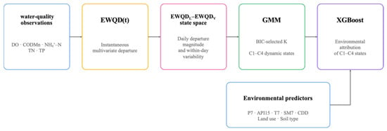
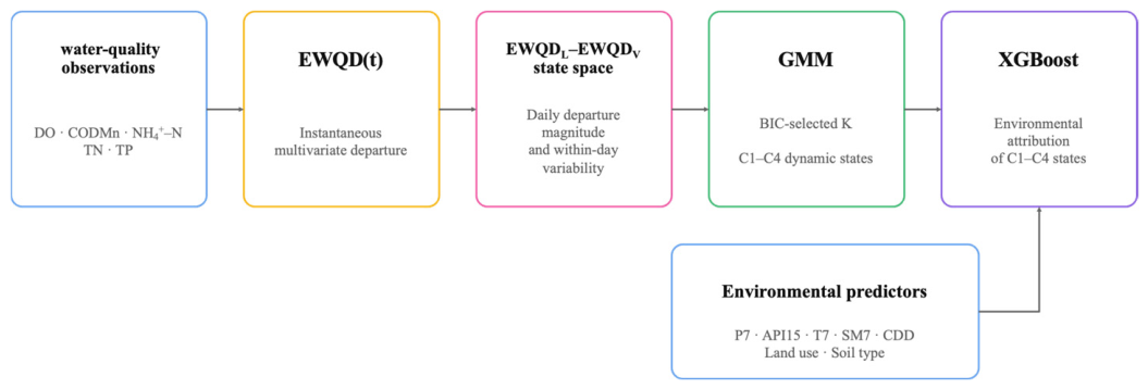
Model performance was evaluated on the independent testing dataset using the overall classification accuracy and macro-averaged F1-score. To further assess model robustness, stratified five-fold cross-validation was performed across the entire dataset while preserving the class distribution in each fold. The reported cross-validation results correspond to the mean and standard deviation of the macro-averaged F1-score across the five validation folds. The overall analytical workflow, from the original 4-h water-quality observations to dynamic-state identification and environmental attribution, is summarized in Figure 1.
Figure 1.
Overview of the analytical workflow for dynamic water quality characterization and environmental attribution.
2.5. Statistical Analysis
All statistical analyses were performed using Python 3.11. Data processing was conducted using NumPy (2.2.6) and Pandas (2.3.3); statistical analyses were performed using SciPy (1.15.3) and scikit-learn (1.7.2); machine learning analyses were implemented using the XGBoost library (3.1.2); and all figures were generated using Matplotlib (3.10.7). The departure states (C1–C4) used in the XGBoost analysis were independently identified by GMM in the two-dimensional EWQDL–EWQDV state space. XGBoost was subsequently used only to relate these predefined states to hydrometeorological and landscape predictors and was not involved in the calculation of EWQD(t), EWQDL, EWQDV, or the identification of the GMM states.
Differences in the daily amplitudes of individual water quality indicators between stable and dynamic station-days were evaluated using the nonparametric Mann–Whitney U test because the variables did not satisfy the assumption of normality. Associations between categorical environmental variables (land use and soil type) and departure states were evaluated using chi-square tests of independence, and Cramér’s V was calculated to quantify the strength of association. Statistical significance was determined at p < 0.05. A station day was classified as dynamic when at least one change in water quality class occurred between consecutive observations. The dynamic day frequency was calculated as the proportion of dynamic station days among all valid station days. Hourly switching frequency was calculated as the proportion of adjacent observation pairs exhibiting a change in water quality class within each hour of the day, and the hour with the highest switching frequency was identified as the peak switching hour. For comparison with EWQDV, an auxiliary daily amplitude metric was calculated. At each 4-h observation, the standardized departure scores of the available water quality variables were first averaged to obtain a mean multivariate departure. The daily amplitude was then calculated as the difference between the maximum and minimum values of this mean departure series within each day.
3. Results
3.1. Characteristics of River Water Temporal Dynamics
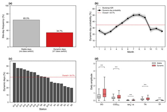
During the study period, 13,088 monitored site-days generated 58,859 adjacent observations, among which 14.0% involved changes in integrated water-quality class (Table 1). Approximately 34.7% of monitored site-days experienced at least one within-day water-quality class transition, whereas the remaining 65.3% remained within a single water-quality class during the day (Figure 2a). Dynamic conditions typically included two within-day class transitions, while the maximum observed frequency reached five transitions within a single day, indicating substantial temporal variability captured by continuous monitoring (Table 1).
Table 1.
Temporal characteristics of river-water dynamics.
Figure 2.
(a) Frequency of stable and dynamic site-days, where dynamic days were defined as days with at least one within-day integrated water-quality class transition. (b) Monthly probability of dynamic conditions. The black line represents the median probability, the grey band indicates the interquartile range (IQR), grey lines represent bootstrap realizations, and the red dashed line denotes the overall mean dynamic-day frequency. (c) Spatial variation in the occurrence of dynamic conditions across the 18 monitoring stations; the red dashed line indicates the overall mean. (d) Comparison of within-day amplitudes of DO, CODMn, NH4+-N, TN, and TP between stable and dynamic days. Boxplots show the median, interquartile range, and whiskers extending to 1.5 × IQR; differences between stable and dynamic days were assessed using the Mann–Whitney U test, with *** indicating p < 0.001.
The occurrence of dynamic conditions exhibited pronounced seasonal variation (Figure 2b). Monthly probabilities remained generally below 25% during winter (December–February), increased progressively during spring, and reached the highest levels during July and August, when approximately 50% of monitored site-days experienced at least one within-day class transition. The occurrence probability subsequently declined during autumn and returned to relatively low levels in winter. Continuous temporal dynamics also varied markedly among monitoring stations (Figure 2c). Across the 18 monitoring stations, the proportion of dynamic site-days ranged from approximately 20% to more than 50%, demonstrating considerable spatial heterogeneity in the temporal stability of river-water quality within the river network. Dynamic conditions were consistently associated with larger within-day fluctuations in water quality (Figure 2d). Daily amplitudes of DO, CODMn, NH4+-N, TN, and TP were all significantly greater during dynamic days than during stable days (p < 0.001). The distributions of daily amplitudes for all five indicators shifted toward higher values under dynamic conditions, confirming that within-day class transitions were accompanied by concurrent increases in the magnitude of water-quality fluctuations across multiple indicators. Collectively, these results demonstrate that high-frequency monitoring captured continuous temporal information describing the occurrence, timing, frequency, spatial distribution, and magnitude of river-water dynamics.
3.2. Water Exposure Patterns
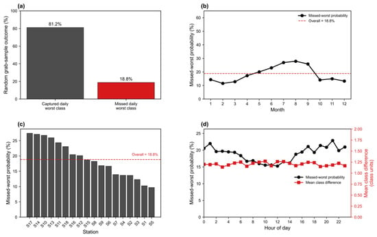
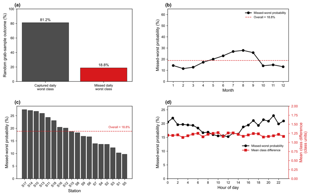
Using the continuous monitoring record as the daily reference, 81.2% of random grab samples successfully captured the daily worst water quality class, whereas 18.8% failed to detect the daily worst condition (Figure 3a). Across all valid observations (71,947 grab samples from 13,088 site-days), the mean class difference among missed observations was 1.2 class units, indicating that missed observations typically underestimated the daily worst water quality condition by approximately one water-quality class. The probability of missing the daily worst water quality class exhibited a pronounced seasonal pattern (Figure 3b). Monthly probabilities ranged from approximately 11–13% during winter to 26–28% during July–August, with the highest values occurring in midsummer. Bootstrap resampling showed consistent seasonal differences, with the interquartile range remaining relatively narrow throughout the year.
Figure 3.
(a) Overall probability that a single grab sample captured or missed the daily worst water quality class. (b) Monthly variation in the probability of missing the daily worst water quality class. (c) Spatial variation in the probability of missing the daily worst water-quality class among the 18 monitoring stations. (d) Hourly variation in the probability of missing the daily worst water-quality class. Mean class difference was calculated only for observations that underestimated the daily worst water-quality class.
Spatial variability was also evident among the 18 monitoring stations (Figure 3c). Station-specific probabilities of missing the daily worst water quality class ranged from approximately 10% to 28%, while the overall mean probability remained 18.8%. Most stations clustered around the overall mean, although several stations consistently exhibited substantially higher or lower probabilities. Hourly analyses revealed clear diurnal variation in the probability of missing the daily worst water quality class (Figure 3d). Although the probability declined to approximately 15–16% around midday, it remained consistently above 15% throughout the entire day and increased again during the late afternoon and evening to more than 20%. In contrast, the mean class difference among missed observations remained relatively stable at approximately 1.1–1.3 class units, indicating that once the daily worst water-quality class was missed, grab sampling typically underestimated the actual daily worst condition by about one water quality class, regardless of sampling time.
3.3. Dynamic Water Quality Indicators
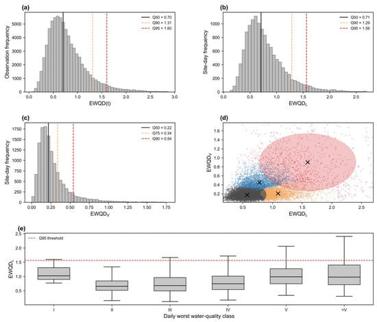
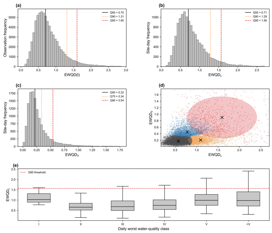
To characterize ecological water quality departure across temporal scales, a three-level EWQD framework was established. At the observation scale, EWQD(t) quantified the instantaneous ecological departure of each 4-h water-quality observation relative to its long-term background (Figure 4a). The distribution of EWQD(t) was strongly right-skewed, with a median value of 0.70, while the Q90 and Q95 thresholds reached 1.31 and 1.60, respectively, indicating that large ecological departures occurred infrequently but contributed disproportionately to extreme events.
Figure 4.
(a) Distribution of the 4-h ecological water-quality departure index. EWQD(t), representing instantaneous ecological departure at the observation scale. (b) Distribution of the daily ecological departure level (EWQDL). (c) Distribution of the daily ecological departure variability (EWQDV). (d) Ecological state space constructed from EWQDL and EWQDV. Four representative ecological states were objectively identified using Gaussian mixture clustering. Crosses indicate cluster centroids, and ellipses denote the robust core region (Q25–Q75) of each ecological state. Colors distinguish the four ecological states: C1 (gray), C2 (orange), C3 (blue), and C4 (red). (e) Distribution of EWQDL across conventional daily worst water-quality classes. The dashed red line denotes the Q95 threshold of EWQDL. Water-quality classes follow GB 3838–2002 [12], where Class I represents the highest quality and <V represents Inferior Class V.
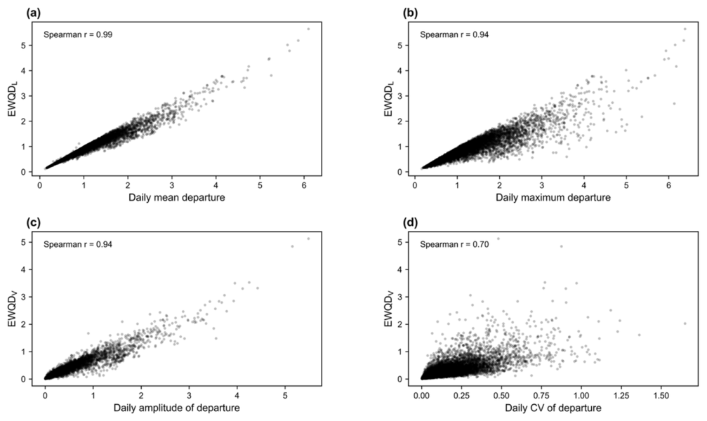
Daily ecological departure was subsequently summarized into two complementary descriptors. EWQDL represented the mean departure level throughout the day, reflecting the overall intensity of ecological stress (Figure A3a,b). EWQDL also exhibited a right-skewed distribution, with a median of 0.71, whereas only 5% of site-days exceeded the Q95 threshold (1.56) (Figure 4b). In contrast, EWQDV described the within-day variability of ecological departure(Figure A3c,d), calculated as the daily amplitude of EWQD(t). EWQDV was concentrated at relatively low values (median = 0.22) but displayed a pronounced long tail, indicating that although most days were characterized by relatively stable ecological conditions, occasional days experienced substantial intraday fluctuations (Figure 4c). EWQDL was highly correlated with both daily mean departure (Spearman r = 0.99) and daily maximum departure (r = 0.94), indicating that it preserved both background and extreme departure information. Likewise, EWQDV showed strong relationships with daily amplitude (r = 0.94) and moderate agreement with the coefficient of variation (r = 0.70), suggesting that it effectively characterized within-day ecological variability while avoiding complete dependence on conventional statistical descriptors.
Combining EWQDL and EWQDV generated a two-dimensional ecological state space (Figure 4d). Gaussian mixture clustering objectively identified four representative ecological water quality states without predefined thresholds. These states represented distinct combinations of ecological departure intensity and temporal variability, ranging from stable background conditions to persistent or highly unstable ecological departures. The resulting state space demonstrated that ecological status cannot be adequately represented by departure intensity alone. Days with comparable EWQDL values frequently exhibited markedly different levels of temporal variability, suggesting that both the magnitude and stability of ecological departure contribute to the characterization of short-term ecological water quality dynamics. EWQDL varied substantially among daily worst water quality classes, with considerable overlap between adjacent classes (Figure 4e). This indicates that the daily worst class alone cannot fully characterize the overall ecological departure during a day, whereas EWQDL provides a continuous measure integrating all intra-day observations.
3.4. Environmental Controls on Dynamic Water Quality
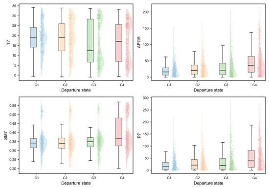
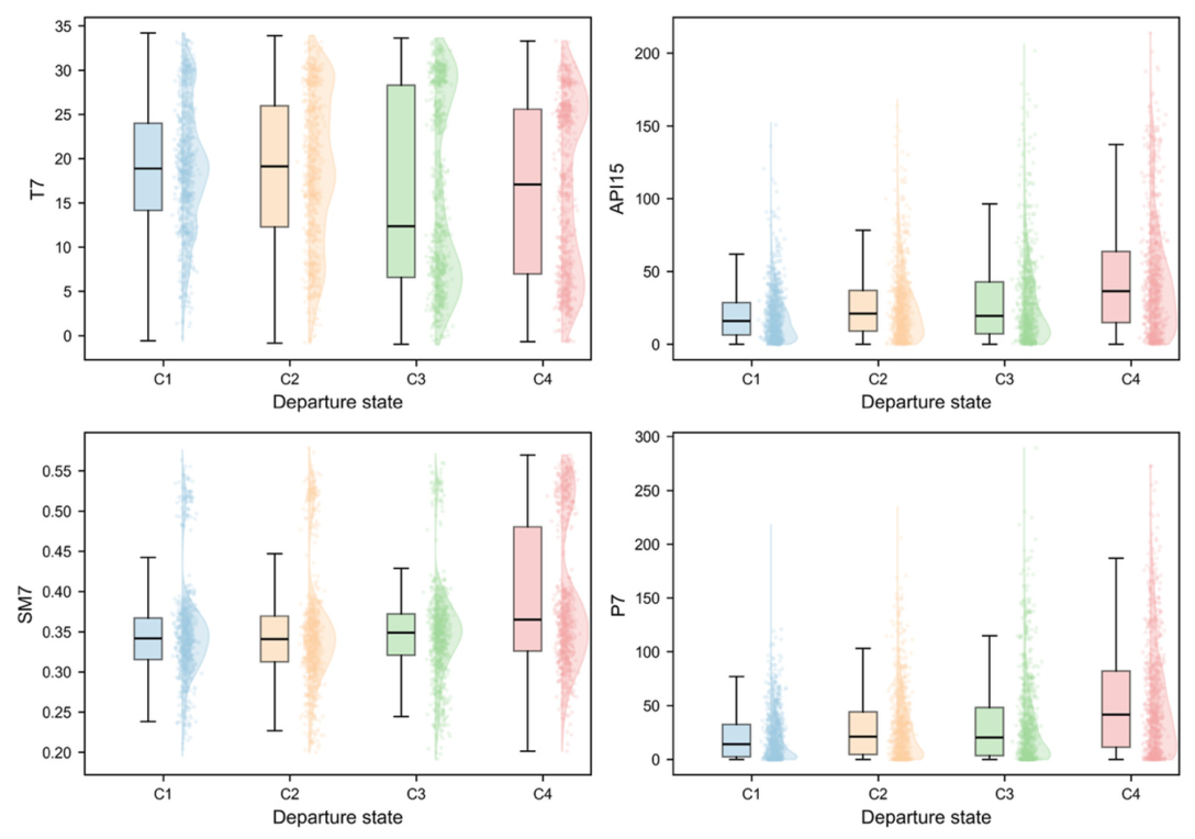
To characterize the environmental settings associated with different departure states, the distributions of major hydro-meteorological variables were compared among the four departure states (C1–C4) (Figure 5). Overall, distinct environmental patterns were observed across the four states. Among the examined variables, antecedent precipitation (API15 and P7) and soil moisture (SM7) exhibited clear differences among departure states, whereas T7 showed substantial overlap, indicating only limited separation when considered individually. Compared with the other states, C4 generally occurred under higher antecedent precipitation and higher soil moisture conditions, whereas C1 was associated with relatively drier environmental conditions characterized by lower API15, P7, and SM7. C2 and C3 exhibited intermediate environmental characteristics, representing transitional conditions between the stable and highly departed states. Although the distributions of individual variables partially overlapped, systematic shifts in their medians and interquartile ranges indicate that the four departure states correspond to distinct hydro-meteorological regimes rather than random partitions of the observations.
Figure 5.
Environmental characteristics of different departure states. Departure states (C1–C4) were identified by Gaussian mixture modelling based on the two-dimensional state vector (L, V), where L represents the departure level, and V represents the temporal variability of EWQD. Specifically, C1 denotes a stable background state (low L–low V), C2 a persistent departure state (high L–low V), C3 an unstable background state (low L–high V), and C4 an unstable departure state (high L–high V).
Landscape background also differed significantly among departure states (Table 2). The composition of departure states varied significantly across land-use types (χ2 = 461.34, p < 0.001, Cramér’s V = 0.11). Paddy fields, urban land, and rural settlements were dominated by the stable state (C1), accounting for 55.3–59.2% of observations. In contrast, other woodland and watercourses exhibited substantially higher proportions of C4, reaching 18.0% and 15.8%, respectively, approximately three times higher than those observed in paddy fields and urban land. These results suggest that landscape background not only influences the occurrence of EWQDs but also alters the composition of different dynamic departure states.
Table 2.
Distribution of departure states across major land use types.
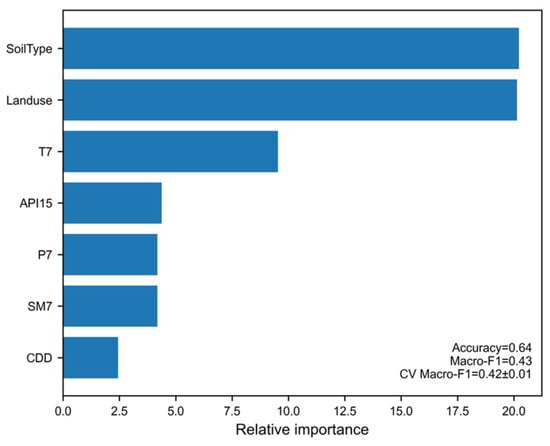
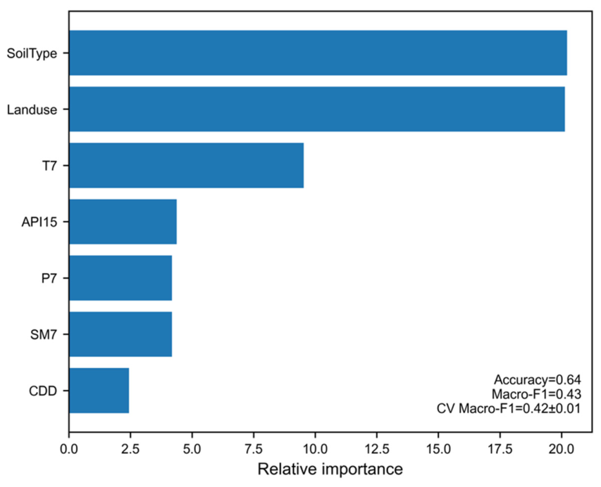
An XGBoost classifier was used to identify the relative importance of environmental controls governing departure-state transitions (Figure 6). Background environmental characteristics (soil type and land use) showed the highest contributions, indicating that spatial heterogeneity establishes the fundamental susceptibility of river systems to different departure states. Although soil type was also retained by the XGBoost model as a background predictor, it was not further summarized because the study area was overwhelmingly dominated by paddy soils (>95%), providing limited discriminatory information. Among the meteorological variables, T7 was the dominant dynamic driver, followed by API15, P7, and SM7, whereas CDD exhibited the weakest contribution.
Figure 6.
Relative importance of environmental drivers.
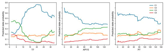
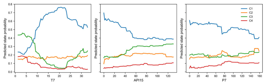
Partial dependence analysis further illustrated how continuous meteorological variables altered the probabilities of different departure states (Figure 7). Increasing antecedent precipitation generally increased the probability of unstable departure states while reducing the occurrence of stable conditions. Temperature exerted a nonlinear influence on state transitions, indicating that moderate thermal conditions favored state persistence whereas higher temperatures promoted shifts toward alternative departure regimes. Overall, the probability responses demonstrate that environmental forcing influences EWQD primarily by altering the likelihood of transitions among L–V departure states rather than through simple linear changes in exposure intensity.
Figure 7.
Effects of environmental drivers on departure state probabilities. Departure states (C1–C4) were identified by Gaussian mixture modelling based on the two-dimensional state vector (L, V), where L represents the departure level, and V represents the temporal variability of EWQD. Specifically, C1 denotes a stable background state (low L–low V), C2 a persistent departure state (high L–low V), C3 an unstable background state (low L–high V), and C4 an unstable departure state (high L–high V).
4. Discussion
4.1. State-Based Characterization of Dynamic Water Quality
The present study demonstrates that river water quality is not adequately represented by departure magnitude alone, but is jointly characterized by the intensity and temporal variability of water-quality departures. Nearly one-third of monitored site-days experienced within-day transitions in water-quality classes, confirming that short-term variability is an intrinsic feature of river water-quality dynamics rather than merely a source of monitoring uncertainty. More importantly, the joint EWQDL–EWQDV state space distinguished water-quality regimes with similar overall departure levels but substantially different temporal behavior. This distinction is important because persistent departure and rapidly fluctuating departure may have similar mean water-quality conditions while representing fundamentally different dynamic regimes.
The dynamic behavior observed in this study is consistent with an increasing body of research based on high-frequency monitoring. River water quality can respond rapidly to rainfall events, hydrological regulation, wastewater discharge, agricultural runoff, and diel biogeochemical processes [13,14], producing substantial fluctuations over hourly to daily time scales [15]. High-frequency monitoring has therefore been widely recognized as an effective approach for detecting transient pollution events, nutrient transport processes, and ecological disturbances that may be overlooked by conventional monitoring programs [16,17]. However, the contribution of the present framework extends beyond detecting these fluctuations. By translating continuous observations into a two-dimensional state space defined by departure level and temporal variability, the framework provides an explicit representation of how water quality evolves between relatively stable and highly dynamic regimes.
This state-based representation complements conventional static assessments. Simulated single-time grab sampling failed to identify a substantial proportion of unfavorable conditions observed within continuous records, illustrating the information loss that can occur when temporally variable systems are represented by isolated observations. More generally, the results indicate that two periods with comparable conventional water-quality classes or average departure levels may differ markedly in their temporal stability. Incorporating temporal variability into water-quality characterization therefore provides information that cannot be recovered from magnitude-based assessment alone and offers a more complete description of short-term river water-quality dynamics.
Several limitations should nevertheless be acknowledged. The proposed framework was developed using routinely monitored physicochemical indicators currently available from continuous monitoring systems. Other water-quality variables that still depend on laboratory analyses were not included and could be incorporated as continuous sensing technologies become more widely available. In addition, the framework was evaluated in a representative plain river-network system in eastern China. Further validation across different climatic regions, hydrological settings, and monitoring networks is required to assess its broader transferability. Future studies could also combine dynamic state characterization with hydrological forecasting and environmental decision-support systems to improve the anticipation and interpretation of rapid water-quality transitions.
4.2. Environmental Controls on Dynamic Water-Quality States
The identification of environmental drivers provides important insights into the mechanisms governing dynamic water-quality states. Our results indicate that hydrometeorological variables, particularly antecedent rainfall, temperature, precipitation, soil moisture, and dry period duration, collectively regulated transitions among dynamic departure states. Similar environmental controls have been widely reported in studies of river water quality [18,19]. Rather than influencing individual water quality variables independently, these environmental factors interact to alter dilution, runoff generation, pollutant transport, biological activity, and in-stream transformation processes, ultimately driving rapid changes in overall water quality conditions [20,21]. Among the identified drivers, antecedent rainfall and temperature exerted the strongest influence on departure state transitions. Previous studies have shown that rainfall affects river water quality through both dilution and the mobilization of accumulated pollutants, whereas antecedent rainfall additionally reflects catchment wetness, groundwater connectivity, and hydrological memory that determine subsequent transport processes [22,23]. Temperature further regulates microbial metabolism, algal activity, dissolved oxygen dynamics, and nutrient transformation, thereby modifying the sensitivity of river water quality to hydrological disturbances [24]. Together, these hydrological and biogeochemical processes generate pronounced antecedent dependence in river water-quality dynamics, consistent with the influence of catchment hydrological memory, explaining why departure state transitions are governed not only by instantaneous meteorological conditions but also by antecedent environmental conditions accumulated over several days. The importance of antecedent rainfall identified in this study therefore suggests that water quality cannot be adequately interpreted from individual rainfall events alone but should instead be considered within the broader context of catchment hydrological memory.
Landscape characteristics further modulated the occurrence of dynamic departure states. Consistent with numerous watershed studies, land use influenced the composition of departure states by altering background pollutant sources and transport pathways [18,25]. Agricultural land generally provides diffuse nutrient inputs, urban areas contribute intermittent point source discharges, while natural landscapes tend to buffer runoff and reduce pollutant delivery to rivers [26,27]. Consequently, land use determines the background susceptibility of river systems to dynamic water quality departures, whereas hydrometeorological forcing primarily determines when state transitions occur. This distinction indicates that environmental drivers operate at different temporal scales, with relatively stable landscape characteristics controlling long-term vulnerability and short-term meteorological conditions triggering rapid transitions among departure states. The environmental dependence of dynamic state transitions also has important implications for water-quality interpretation and monitoring. The probability of rapid transitions increased under combinations of antecedent rainfall, temperature, soil moisture, and rainfall conditions, indicating that the representativeness of individual water-quality observations depends partly on the hydrometeorological context in which they are collected. Fixed-interval monitoring may therefore provide uneven information across environmental conditions, with a greater likelihood of overlooking short-lived departures during periods of high transition probability. Dynamic-state information could support adaptive monitoring by identifying environmental conditions under which additional observations are most informative, rather than simply increasing sampling frequency uniformly throughout the year. More broadly, incorporating environmental controls into dynamic water-quality characterization may help distinguish persistent background departures from transient disturbance-driven states.
Several limitations should also be acknowledged. The environmental drivers analyzed in this study primarily represent climatic and watershed controls and do not explicitly incorporate upstream water management, pollutant discharge schedules, or hydraulic regulation, all of which may further influence short-term river water dynamics. Future studies should integrate hydrological models, continuous environmental monitoring, and environmental forecasting to further improve dynamic water quality characterization and support adaptive water quality management under increasingly variable environmental conditions.
5. Conclusions
This study integrated EWQDL and EWQDV to establish water-quality departure states for characterizing temporal dynamics from continuous river monitoring data. In the Hangjiahu Plain, water-quality dynamics varied considerably across months, with the most frequent fluctuations occurring in July and August. Overall, 34.7% of monitored site-days experienced within-day water-quality class transitions. A grab-sampling analysis based on the continuous monitoring records showed that single-time observations failed to capture the daily worst water-quality class in 18.8% of cases, underestimating the worst condition by an average of 1.2 classes. The probability of missing the daily worst condition varied across seasons and hours of the day, with the highest risk occurring in summer. Short-term shifts in water-quality states were primarily associated with hydrometeorological factors, particularly antecedent rainfall and temperature, while land use regulated the background susceptibility of river systems to water-quality departures.
The framework established in this study provides a practical approach for interpreting continuous river water-quality observations. By integrating continuous monitoring with environmental drivers, it enables dynamic characterization of water-quality states and facilitates the identification of periods with an elevated likelihood of short-term deterioration. Rather than relying solely on fixed-interval observations, this framework supports more representative interpretation of water-quality dynamics by accounting for temporal variability and environmental memory. As continuous monitoring technologies become increasingly widespread, such dynamic characterization frameworks may complement existing regulatory assessment approaches and provide additional information for water-quality assessment, environmental management, and early warning of transient deterioration events.
Author Contributions
Writing—original draft preparation, Y.C. (Yike Chen); Writing—review and editing and Conceptualization, Y.C. (Yanbing Chi); funding acquisition, P.L. All authors have read and agreed to the published version of the manuscript.
Funding
This research was supported by Huzhou Science and Technology Program Project (No. 2023GZ70) and Zhejiang Provincial Ecological Environment Research and Achievement Promotion Project (2025HT0024).
Data Availability Statement
The data presented in this study are available on request from the corresponding author due to privacy.
Conflicts of Interest
The authors declare no conflicts of interest.
Appendix A
Figure A1.
Location of the study area.
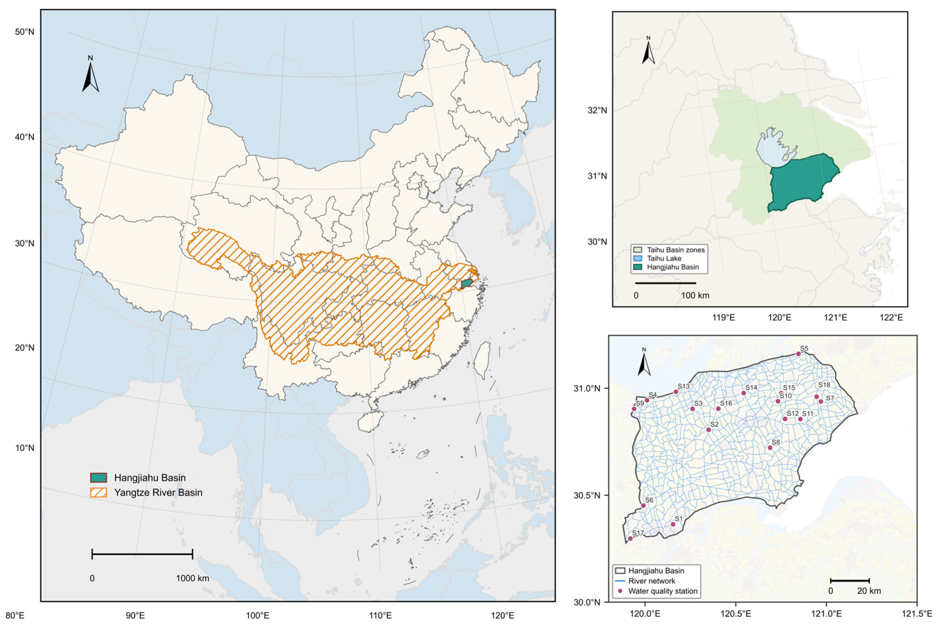
Figure A2.
Seasonal reference states of water quality indicators. Vertical lines indicate the seasonal median concentrations used as the corresponding reference states.
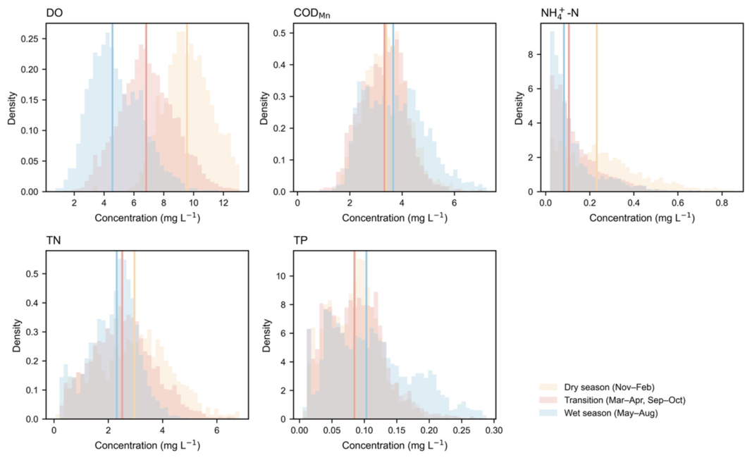
Figure A3.
(a) Relationship between daily mean departure and EWQDL. (b) Relationship between daily maximum departure and EWQDL. (c) Relationship between daily departure amplitude and EWQDV. (d) Relationship between the daily coefficient of variation (CV) of departure and EWQDV. Spearman correlation coefficients are shown in each panel.
References
- Dudgeon, D.; Arthington, A.H.; Gessner, M.O.; Kawabata, Z.-I.; Knowler, D.J.; Lévêque, C.; Naiman, R.J.; Prieur-Richard, A.-H.; Soto, D.; Stiassny, M.L.J.; et al. Freshwater biodiversity: Importance, threats, status and conservation challenges. Biol. Rev. 2006, 81, 163–182. [Google Scholar] [CrossRef] [Scilit] [PubMed]
- Rode, M.; Wade, A.J.; Cohen, M.J.; Hensley, R.T.; Bowes, M.J.; Kirchner, J.W.; Arhonditsis, G.B.; Jordan, P.; Kronvang, B.; Halliday, S.J.; et al. Sensors in the Stream: The High-Frequency Wave of the Present. Environ. Sci. Technol. 2016, 50, 10297–10307. [Google Scholar] [CrossRef] [Scilit] [PubMed]
- Kirchner, J.W.; Feng, X.; Neal, C.; Robson, A.J. The Fine Structure of Water-quality Dynamics: The (High-frequency) Wave of the Future. Hydrol. Process. 2004, 18, 1353–1359. [Google Scholar] [CrossRef] [Scilit]
- Bowes, M.J.; Jarvie, H.P.; Halliday, S.J.; Skeffington, R.A.; Wade, A.J.; Loewenthal, M.; Gozzard, E.; Newman, J.R.; Palmer-Felgate, E.J. Characterising Phosphorus and Nitrate Inputs to a Rural River Using High-Frequency Concentration–Flow Relationships. Sci. Total Environ. 2015, 511, 608–620. [Google Scholar] [CrossRef] [Scilit] [PubMed]
- Javed, A.; Hamshaw, S.D.; Lee, B.S.; Rizzo, D.M. Multivariate Event Time Series Analysis Using Hydrological and Suspended Sediment Data. J. Hydrol. 2021, 593, 125802. [Google Scholar] [CrossRef] [Scilit]
- Tiyasha; Tung, T.M.; Yaseen, Z.M. A Survey on River Water Quality Modelling Using Artificial Intelligence Models: 2000–2020. J. Hydrol. 2020, 585, 124670. [Google Scholar] [CrossRef] [Scilit]
- Varadharajan, C.; Appling, A.P.; Arora, B.; Christianson, D.; Hendrix, V.; Kumar, V.; Lima, A.R.; Mueller, J.; Oliver, S.K.; Ombadi, M.; et al. Can Machine Learning Accelerate Process Understanding and Decision-Relevant Predictions of River Water Quality? Hydrol. Process. 2022, 36, e14565. [Google Scholar] [CrossRef] [Scilit]
- Rozemeijer, J.; Jordan, P.; Hooijboer, A.; Kronvang, B.; Glendell, M.; Hensley, R.; Rinke, K.; Stutter, M.; Bieroza, M.; Turner, R.; et al. Best Practice in High-Frequency Water Quality Monitoring for Improved Management and Assessment; a Novel Decision Workflow. Environ. Monit. Assess. 2025, 197, 353. [Google Scholar] [CrossRef] [Scilit] [PubMed]
- Lawson, L.; Jackson, D.A. Water Quality Patterns in At-Risk Fish Habitat: Assessing Frequency and Cumulative Duration of Chloride Guideline Exceedance during Early Life Stages of an Endangered Fish. Ecol. Indic. 2024, 168, 112707. [Google Scholar] [CrossRef] [Scilit]
- Mebane, C.A. The Capacity of Freshwater Ecosystems to Recover from Exceedences of Aquatic Life Criteria. Environ. Toxicol. Chem. 2022, 41, 2887–2910. [Google Scholar] [CrossRef] [Scilit] [PubMed]
- Wang, Z.; Shi, B.; Osmond, P.; Zhang, K. Multimodal Deep-Learning–Driven Water-Quality Forecasting and Scenario Assessment: Shifting from Reactive Monitoring to Proactive Basin Management. J. Hydrol. 2026, 675, 135554. [Google Scholar] [CrossRef] [Scilit]
- GB 3838—2002; Environmental Quality Standards for Surface Water. Standardization Administration of the People’s Republic of China: Beijing, China, 2002.
- van Vliet, M.T.H.; Thorslund, J.; Strokal, M.; Hofstra, N.; Flörke, M.; Macedo, H.E.; Nkwasa, A.; Tang, T.; Kaushal, S.S.; Kumar, R.; et al. Global River Water Quality under Climate Change and Hydroclimatic Extremes. Nat. Rev. Earth Environ. 2023, 4, 687–702. [Google Scholar] [CrossRef] [Scilit]
- Li, X.; Yang, Y.; Zhou, X.; Liu, L.; Yang, Y.; Han, S.; Zhang, Y. Impact of Water Productivity and Irrigated Area Expansion on Irrigation Water Consumption and Food Production in China in Last Four Decades. Agric. Water Manag. 2024, 304, 109100. [Google Scholar] [CrossRef] [Scilit]
- Heathwaite, A.L.; Bieroza, M. Fingerprinting Hydrological and Biogeochemical Drivers of Freshwater Quality. Hydrol. Process. 2021, 35, e13973. [Google Scholar] [CrossRef] [Scilit]
- Bieroza, M.; Acharya, S.; Benisch, J.; Ter Borg, R.N.; Hallberg, L.; Negri, C.; Pruitt, A.; Pucher, M.; Saavedra, F.; Staniszewska, K.; et al. Advances in Catchment Science, Hydrochemistry, and Aquatic Ecology Enabled by High-Frequency Water Quality Measurements. Environ. Sci. Technol. 2023, 57, 4701–4719. [Google Scholar] [CrossRef] [Scilit] [PubMed]
- Burns, D.A.; Pellerin, B.A.; Miller, M.P.; Capel, P.D.; Tesoriero, A.J.; Duncan, J.M. Monitoring the Riverine Pulse: Applying High-Frequency Nitrate Data to Advance Integrative Understanding of Biogeochemical and Hydrological Processes. WIREs Water 2019, 6, e1348. [Google Scholar] [CrossRef] [Scilit]
- Qiu, M.; Wei, X.; Hou, Y.; Spencer, S.A.; Hui, J. Forest Cover, Landscape Patterns, and Water Quality: A Meta-Analysis. Landsc. Ecol. 2023, 38, 877–901. [Google Scholar] [CrossRef] [Scilit]
- Noriega Giménez, J.; Saavedra Cifuentes, E.; Vincent, A.E.S.; Packman, A.I. Subsurface Conditions and Hydrologic Accumulation Drive Stream Connectivity and Flow Intermittency in Urban River Networks. Commun. Earth Environ. 2026, 7, 511. [Google Scholar] [CrossRef] [Scilit]
- Li, Z.; Fang, K.; Wu, H.; Gao, X.; Wu, F. Disentangling Multi-Scale Impacts on Surface Water Quality: A Hierarchical Modeling Approach. Ecol. Indic. 2025, 178, 114061. [Google Scholar] [CrossRef] [Scilit]
- Zhang, H.; Sun, H.; Li, J.; Li, Y.; Zhang, L.; Zhao, R.; Hu, X.; Ren, N. Natural and Anthropogenic Imprints on Seasonal River Water Quality Trends across China. npj Clean. Water 2025, 8, 49. [Google Scholar] [CrossRef] [Scilit]
- Gorgij, A.D.; Moayeri, M.M. Proposing a Novel Method for the Irrigation Water Quality Assessment, Using Entropy Weighted Method, Entitled: “EIWQI”. Environ. Earth Sci. 2023, 82, 462. [Google Scholar] [CrossRef] [Scilit]
- Pourfallah Koushali, H.; Mastouri, R.; Khaledian, M.R. Impact of Precipitation and Flow Rate Changes on the Water Quality of a Coastal River. Shock. Vib. 2021, 2021, 6557689. [Google Scholar] [CrossRef] [Scilit]
- Zhi, W.; Ouyang, W.; Shen, C.; Li, L. Temperature Outweighs Light and Flow as the Predominant Driver of Dissolved Oxygen in US Rivers. Nat. Water 2023, 1, 249–260. [Google Scholar] [CrossRef] [Scilit]
- Xu, Q.; Wang, P.; Shu, W.; Ding, M.; Zhang, H. Influence of Landscape Structures on River Water Quality at Multiple Spatial Scales: A Case Study of the Yuan River Watershed, China. Ecol. Indic. 2021, 121, 107226. [Google Scholar] [CrossRef] [Scilit]
- Chen, G.; Liu, L.; Wang, W.; Wang, R.; Li, Y.; Tang, X.; Li, X. Effectiveness of Best Management Practices for Non-Point Source Pollution in Intensively Managed Agricultural Watersheds. J. Clean. Prod. 2025, 495, 145076. [Google Scholar] [CrossRef] [Scilit]
- Liu, L.; Ouyang, W.; Liu, H.; Zhu, J.; Fan, X.; Zhang, F.; Ma, Y.; Chen, J.; Hao, F.; Lian, Z. Drainage Optimization of Paddy Field Watershed for Diffuse Phosphorus Pollution Control and Sustainable Agricultural Development. Agric. Ecosyst. Environ. 2021, 308, 107238. [Google Scholar] [CrossRef] [Scilit]

Disclaimer/Publisher’s Note: The statements, opinions and data contained in all publications are solely those of the individual author(s) and contributor(s) and not of MDPI and/or the editor(s). MDPI and/or the editor(s) disclaim responsibility for any injury to people or property resulting from any ideas, methods, instructions or products referred to in the content. |
© 2026 by the authors. Licensee MDPI, Basel, Switzerland. This article is an open access article distributed under the terms and conditions of the Creative Commons Attribution (CC BY) license.