Root-Zone Moisture Realized During a Compound Dry–Hot Event, Not Irrigation Persistence, Determines the Resilience of Cropland Carbon–Water Productivity in the Guanzhong Plain, China

Ju, Mengchen; Sun, Jun; Yang, Yuanyuan; Huo, Haixia

doi:10.3390/w18172149

Abstract

Warming is making drought and heat co-occur more often, intensifying compound stress on cropland in northern China’s drylands, where water scarcity makes further irrigation expansion untenable. On the Guanzhong Plain, a major grain-producing region, it remains unclear which irrigation conditions buffer cropland carbon–water productivity—the carbon assimilated per unit of water consumed—against such events. Using growing-season (March–October) remote sensing for 2016–2024, we identified the 2022 compound drought–heat event pixel by pixel and classified cropland as stable rainfed, transitional/mixed, or stable high-coverage irrigation from the pre-event (2016–2020) irrigated-area fraction and its persistence. In 2022, 88.9% of cropland experienced at least one compound dry–hot day, with dry–hot overlap 2.4 times the independence expectation. After balancing climate, terrain, soil, spatial position, and subpixel cropland fraction, stable high-coverage irrigation held no advantage in event-year resistance, post-event recovery, or overall resilience. Carbon assimilation remained above its pre-event level while carbon–water productivity fell, so the event cost water-use efficiency rather than carbon. Event-period root-zone soil-moisture change ranked first, and irrigated-area fraction last, among twelve random-forest predictors of resistance. We flagged 6722.3 km² of cropland for water-use audits and 2418.1 km² for supplemental irrigation; limited water should be allocated by realized moisture status, exposure, and resilience, not by irrigability.

Keywords:

compound drought–heat event; irrigation persistence; carbon–water productivity; resistance; recovery; precision irrigation

1. Introduction

Climate warming is altering the way drought and high temperature occur together, and compound events have consequently become a central topic in agricultural climate-risk research [1,2]. Their joint impact exceeds the linear sum of either driver acting alone: warming raises atmospheric evaporative demand, whereas soil-water deficit suppresses stomatal conductance and carbon assimilation, so crops lose their water supply precisely when transpirational cooling is most needed and losses are amplified [3,4]. Across the agricultural regions of northern China, both the number of days and the spatial extent of concurrent hot and dry conditions during the growing season have continued to increase [5,6]. In 2022, many parts of the country experienced record-breaking compound heatwave and drought conditions, with significant negative anomalies over more than half of the vegetated area, and the Guanzhong Plain endured a persistently hot and dry summer in the same year [7,8]. The recurrence of such events is no longer a matter of probability; how to sustain the productive capacity of cropland when they occur has become the most pressing question for regional agricultural adaptation.

Irrigation is the most direct means of attenuating this risk. It lowers the sensitivity of crop yield to temperature and precipitation anomalies, moderates heat exposure by increasing latent heat flux, and in drylands raises evapotranspiration, canopy greenness, and yield, simultaneously [9,10,11]. Its adaptive capacity is nevertheless bounded by the water available, so expanding irrigated area is not a viable way to resolve the risk where water is scarce [12]. The more useful question is which irrigation conditions sustain higher carbon assimilation for a given amount of water consumed—that is, which conditions sustain cropland carbon–water productivity [13,14]. No consistent answer has yet emerged, for four reasons. First, most studies delineate compound events using climate indices aggregated to the season or the month; heat and water deficit occurring at different times can still yield a high index value, so whether drought and heat truly coincided cannot be confirmed [15]. Second, existing remote-sensing irrigation products report either the areal fraction of irrigated land within a pixel or a binary irrigated/non-irrigated label. They carry no information on the amount, frequency, or timing of water applied, and agreement among products over the Yellow River Basin is limited [16,17,18].

Most regional comparisons still assign treatment groups from binary labels and ignore the interannual persistence of irrigation coverage, so cropland that is reliably irrigable and cropland that is irrigated only intermittently fall into the same group, which dilutes the true contrast. Third, many studies equate the change in output during the event year with resilience and do not separate event-year resistance, post-event recovery, and overall resilience across a complete event cycle. These three components can point in opposite directions, and recovery is systematically inflated by a depressed event-year denominator [19,20,21]. Fourth, carbon–water productivity is obtained by dividing one remotely sensed productivity product by an independent evapotranspiration product, so a between-group difference derived from a single product pair cannot be checked for reproducibility of sign [22,23]. Even where a difference is real, irrigated and rainfed cropland differ systematically in terrain and background climate, and their joint spatial distribution is a source of confounding. It also remains unresolved whether irrigation acts as a state in its own right or through the moisture conditions that crops actually experience [24].

These constraints are particularly acute in Guanzhong. Water resources there are scarce; agricultural water use has long depended on the limited surface runoff and groundwater of the Wei River Basin, and climate change is expected to intensify streamflow depletion and the imbalance between supply and demand [25]. The volume available for reallocation is already close to its ceiling, yet compound drought–heat events continue to become more frequent. Because the region cannot resolve the risk by expanding the scale of irrigation, the remaining room lies in using the existing water more precisely. Guanzhong also offers the conditions needed to address the gaps identified above. The five municipalities of Xi’an, Xianyang, Baoji, Weinan, and Tongchuan share a broadly uniform regional climate, yet they contain contiguous long-established irrigation districts along the Wei River corridor, rainfed dryland farming on the loess tablelands and the piedmont transition belt, and, between the two, zones in which irrigation coverage fluctuates from year to year. Together these form a continuous gradient of irrigation persistence and provide an uncommon opportunity for between-class comparison within a single event.

Here we examine cropland across the five Guanzhong municipalities during the 2022 compound drought–heat event. We ask which irrigation conditions effectively weaken the impact of a compound event on cropland carbon–water productivity, and we use the answer to set a regional order of priority for allocating limited water. The analysis proceeds in four steps. We first determine, pixel by pixel and at a daily time step, whether drought and heat co-occurred, then we delimit the event period, and quantify exposure intensity. We then classify comparable cropland types using only the pre-event irrigated-area fraction and its interannual persistence. Next, we decompose and compare resistance, recovery, and overall resilience, and test whether the between-class differences should be attributed to irrigability or to the root-zone moisture status actually realized during the event. Finally, we combine resilience with water-use response to derive a regional order of priority for water-use audits and supplemental irrigation.

2. Materials and Methods

2.1. Study Area, Analysis Grid, and Multi-Source Observations

The study area comprises the administrative territories of the five municipalities of Xi’an, Xianyang, Baoji, Weinan, and Tongchuan in the Guanzhong region of Shaanxi Province, China. It extends from 106.31° to 110.61° E and from 33.58° to 35.85° N, covering 55,444.6 km². The analysis grid consists of 957 × 507 cells of 500 m with a cell spacing of 0.004491576° in EPSG:4326. The cropland mask retains every cell whose modal land cover from the Moderate Resolution Imaging Spectroradiometer (MODIS) on board the Terra and Aqua satellites (National Aeronautics and Space Administration, Washington, DC, USA) for 2016–2020 is cropland or the cropland/natural-vegetation mosaic, giving 145,948 cells [26,27]. Because the mosaic class contains only 40–60% cropland by product definition, the cropland class of ESA WorldCover was aggregated to the analysis grid to give a subpixel cropland fraction for every cell [28]. That fraction was derived from the 2021 v200 map, and its correlation with the 2020 v100 map is 0.955.

The analysis period is 2016–2024, and the growing season is defined as 1 March to 31 October. The primary carbon and water fluxes are the gross primary productivity, total evapotranspiration, and vegetation transpiration of PML-V2.2a, hereafter GPP, ET, and Ec, respectively [22,29]. An independent series was assembled from MOD17A2HGF and MOD16A2GF to evaluate product dependence [23,30,31]. Pixel-level response and state variables were aggregated over the growing season, whereas the irrigation, soil, and terrain attributes are pre-event multi-year or static quantities. Processing details for every product are given in Table 1, and no downscaling was applied at any stage [32,33,34].

Table 1. Version, source, quality control, temporal processing, resampling, and use of each dataset.

2.2. Pre-Event Irrigation Classes and Definition of the Treatment Variable

The irrigation classes were determined entirely from pre-event information. The primary criterion was the annual irrigated-area fraction reported by CIrrMap250 for 2016–2020, a product that gives the share of irrigated land within each 250 m pixel and has been checked against irrigation statistics and water-withdrawal records [16]. For every cropland pixel we computed the five-year mean irrigated-area fraction together with the proportion of years in which irrigation coverage reached 50% or more, hereafter persistence, and used these two quantities to define three cropland classes (Table 2). The treatment variable is therefore the pre-event coverage of irrigated area and its interannual persistence, and not the amount, frequency, timing, method, or source of applied water. The irrigated-area estimates of this product explain roughly 50–60% of the variance in national irrigation withdrawals [16], so what they characterize is the spatial pattern of pre-event irrigability.

Table 2. Definition, independent verification criterion, agreement, and mapped area of the pre-event irrigation classes.

Three independent procedures were used to verify the classification. First, the annual binary irrigation maps of IrriMap_CN, which play no part in constructing the classes, served as an independent criterion [17]; agreement with the two stable classes was 88.6% and 73.8%. Second, because the suitability of irrigation products differs across the Yellow River Basin [18,39], the two thresholds were varied jointly between 10% and 25% and between 50% and 70%, giving six combinations. Third, we constructed a core sample of 45,779 pixels for which the two products agree and the subpixel cropland fraction is at least 0.6. The main results are based on the full sample, the outcome of each procedure is reported for every dimension of the analysis, and the matched results specific to the core sample are reported separately in Table S12.

The agricultural water supply of the five Guanzhong municipalities in 2022, as recorded in the Shaanxi Water Resources Bulletin, shows no interruption of regional irrigation supply in that year [40]. The between-class comparison is therefore defined as a contrast between pre-event irrigable conditions and not between volumes of water actually received. Stable rainfed and stable high-coverage irrigation are the two most clearly defined end members, and the binary comparison and covariate balancing are restricted to them. Transitional/mixed irrigation is the residual class; it arises both from interannual fluctuation in coverage and from subpixel mixing, and it enters only the continuous exposure–response estimation and the regional screening zonation.

2.3. Pixel-Wise Identification of the Compound Drought–Heat Event and Quantification of Exposure

Drought was identified at a daily time step for every grid cell using the Meteorological Drought Composite Index (MCI). This index is prescribed by the Chinese national standard Grades of Meteorological Drought and underpins the operational drought monitoring of the China Meteorological Administration; its weights, parameters, and grade thresholds are listed in Table S6 [41]. MCI was preferred over purely precipitation-based indices for two reasons: its most heavily weighted term, the relative moisture index, already incorporates evaporative demand, and the growing-season precipitation anomaly over Guanzhong in 2022 was close to zero, so the water deficit was driven mainly by evaporative demand. Detection was carried out on the native 0.05° CHIRPS grid, which contains more than 4000 cells over the study area and thus permits gamma parameters to be fitted for every cell and every calendar day; the results were then replicated from the parent cell onto the 500-m analysis grid.

Heat was identified independently on the same grid and at the same time step. A hot day is a day on which the daily maximum air temperature exceeds the 90th percentile for that calendar day over 1991–2020, with the climatology estimated within a centered window of ±7 days [42]. Because such a window admits the seasonal cycle of neighboring calendar days, we ran a parallel check using thresholds derived from the same calendar day alone [43]. The intersection of the two criteria defines a compound dry–hot day. Isolated compound days carry no process meaning, so only runs of three or more consecutive days were retained, and multiple runs within one season were combined as a union [6,15,44]. At the event level we additionally applied a heatwave-conditioned definition of drought: a run of at least three consecutive hot days embedded within a drought period of at least five days at moderate grade or worse, with episodes separated by no more than three days merged (Table S6) [15]. The 2022 event period identified in this way agrees with a regional study of the same episode [8].

Exposure intensity was quantified at two temporal scales. Event-period exposure was obtained by summing, over all compound dry–hot days, the daily product of drought intensity and normalized heat intensity [45]; heat intensity was normalized by the interquartile range of the daily maximum temperature during the reference-period growing seasons:

S = \sum_{d \in D} (- {MCI}_{d}) \cdot \frac{T_{\max, d} - T_{25}}{T_{75} - T_{25}}

(1)

where S is the event-period cumulative severity, D is the set of all compound dry–hot days at that grid cell in the given year, MCI_d is the value of the Meteorological Drought Composite Index on day d, so that −MCI_d is the drought intensity, T_max,d is the daily maximum air temperature on day d, and T₂₅ and T₇₅ are the quartiles of the daily maximum temperature during the reference-period growing seasons, equal to 18.94 and 29.25 °C, respectively. Because normalization is scaled to the heat intensity of a typical growing season, hot days in early spring contribute little, and no truncation at zero is applied. Equation (1) automatically merges separate episodes within a season and returns zero, rather than an undefined value, at cells with no compound dry–hot day in that year.

Exposure at the growing-season scale is described by the compound drought–heat exposure intensity index (CDHEI). Relative to the 1991–2020 climatology, this index combines with equal weights the standardized anomalies of growing-season total precipitation, mean daily maximum temperature, vapor pressure deficit (VPD), and total potential evapotranspiration (PET):

C D H E I = z_{Tmax} + z_{PET} + z_{VPD} - z_{P}

(2)

where z_Tmax, z_PET, z_VPD, and z_P are the standardized anomalies of the growing-season mean daily maximum temperature, total potential evapotranspiration, vapor pressure deficit, and total precipitation, respectively, each expressed relative to the 1991–2020 climatology. Its three heat- and evaporative-demand terms are mutually correlated rather than independent sources of information, so the CDHEI of Equation (2) is used only as a monotonic ranking of exposure intensity and not as a probabilistic measure of severity.

The two definitions were applied in parallel at three points in the analysis—covariate balancing, estimation of the exposure–response relationship, and the random forest—and agreement or disagreement between them is reported as found. Event-period cumulative severity was adopted as the main setting for two reasons: it is summed over all compound dry–hot days of the growing season and therefore matches the temporal support of the growing-season response variables, and by construction it guarantees that water deficit and heat stress occurred on the same day. An event year must satisfy the daily and the growing-season criteria simultaneously; the latter requires a negative standardized anomaly of growing-season precipitation, a positive standardized anomaly of maximum temperature, and a positive standardized anomaly of either VPD or PET.

2.4. Carbon–Water Productivity and the Three-Component Resilience Framework

Water productivity in this study refers specifically to remotely sensed carbon–water productivity (CWP), that is, the carbon assimilated per unit of water consumed. It is not the same quantity as yield-based water productivity, which divides grain yield by irrigation supply, and the two are never used interchangeably here. Two definitions were carried in parallel in Equation (3): the transpiration-based definition, CWP_Ec, describes the coupling between carbon assimilation and physiological water use, whereas the definition based on total evapotranspiration, CWP_ET, describes total water-use efficiency at the ecosystem scale:

{CWP}_{Ec} = \frac{GPP}{E_{c}}, {CWP}_{ET} = \frac{GPP}{ET}

(3)

where CWP_Ec and CWP_ET are the transpiration-based and evapotranspiration-based carbon–water productivity, GPP is gross primary productivity, Ec is vegetation transpiration, and ET is total evapotranspiration, which comprises vegetation transpiration, soil evaporation, and interception evaporation. A lower bound of 0.01 mm was imposed on both denominators before division to prevent division by zero. The three fluxes of PML-V2.2a originate in a single model framework, whereas the independent metric is the ratio of MOD17 gross primary productivity to MOD16 total evapotranspiration [22,23,29]. All three metrics were computed in parallel at each of the steps above, whereas the estimation of the exposure–response relationship, the random forest, and the regional screening zonation use transpiration-based resistance as their sole response variable.

Following the resistance–recovery decomposition framework [19,20], we took the 2016–2021 mean as the pre-event baseline, 2022 as the event state, and the 2023–2024 mean as the post-event state, and used Equation (4) to define three resilience components for any strictly positive metric X:

R_{t} = \frac{X_{event}}{X_{pre}}, R_{c} = \frac{X_{post}}{X_{event}}, R_{s} = \frac{X_{post}}{X_{pre}}

(4)

where R_t, R_c, and R_s denote resistance, recovery, and overall resilience, and X_pre, X_event, and X_post are the values of the metric averaged over the pre-event baseline, the event year, and the post-event window, respectively. A resistance of 1 indicates that the event-year state was maintained at the baseline level, an overall resilience of 1 indicates that the post-event state returned to the baseline, and a recovery greater than 1 indicates that the post-event state exceeded the event-year state. The three components are used strictly separately and are never referred to collectively as resilience [21]. Because recovery takes the event-year state as its denominator, a larger event-year decline inflates its value.

The two windows are deliberately of unequal length. The baseline spans six years so that the normal state is estimated with adequate precision, since a shorter baseline would allow a single anomalous year to dominate it. The two-year post-event window is set by the data record: the primary response product ends in late 2024, and a further compound event of moderate grade occurred in 2025, which therefore does not provide a clean recovery year. Neither 2023 nor 2024 satisfied the event-year criteria; localized compound events affected 27.3% and 37.6% of cropland in the two years, and their seasonal climate backgrounds were opposite in sign. The two-year mean was therefore adopted as the main setting, and results using each single year as the recovery state are reported separately.

2.5. Statistical Inference, Mechanistic Evaluation, and Regional Screening Zonation

The approximately 146,000 pixels are not independent observations. All between-class differences were therefore obtained by block bootstrap, with the class-area-weighted mean within 20 km spatial blocks in an Albers equal-area projection as the unit of inference; this block size exceeds the native grid of the main reanalysis inputs and thereby weakens local dependence [46,47]. Aside from the difference in its original units, every balanced difference is also reported as a standardized difference in units of the full-sample standard deviation and as a paired effect size. A guard interval of 0.2–3.0 was imposed jointly on the nine ratio metrics to exclude artifacts produced by denominators approaching zero; three alternative intervals and the associated removal audit are given in Table S7.

Irrigation class and site conditions are jointly distributed in space, so the between-class differences were additionally re-estimated after covariate balancing [48,49,50]. The temporal attribution of the covariates was kept strict. Precipitation, maximum temperature, and root-zone soil moisture are growing-season means for the pre-event years 2016–2021; soil properties, terrain, and planar coordinates are time-invariant; and exposure intensity is the only variable taken from the event year. Pre-event rather than event-year soil moisture was used because the latter is influenced by irrigation and lies on the causal pathway through which irrigation acts on resilience; balancing on it is a textbook case of bad control and would remove part of the very association to be estimated [51]. Exposure intensity, by contrast, is derived from climate data that do not represent irrigation and is exogenous with respect to irrigation status, so balancing on it amounts to equalizing meteorological exposure.

An eleventh covariate, the subpixel cropland fraction aggregated from 10 m land cover, was added on this basis. This variable reflects the geomorphic contrast between the dissected loess tablelands and the contiguous alluvial plain; it lies upstream of irrigability and belongs with elevation and slope as a source of confounding rather than as a mediator. All between-class differences were therefore estimated in parallel under the ten-covariate and the eleven-covariate specifications and repeated on three subsamples with cropland fractions of at least 0.5, 0.6, and 0.8 and on the core sample, forming a 5 × 2 factorial design. Matching parameters, sensitivity settings, and the treatment of multiple comparisons are listed together in Table S7.

The exposure–response relationship was estimated with linear regression and with single-breakpoint segmented regression, taking block-level class means as the unit of analysis [52,53]. The three classes were fitted separately, and the difference in slope between the two stable classes was tested over their common exposure support. Because only one compound-stress year occurred within the study period, this analysis characterizes the spatial variation in exposure and response within a single event [54]. Random forests were used to assess the incremental spatial predictive information that candidate variables carry about resistance, not to redefine the irrigation classes [55], and generalization was assessed by five-fold grouped cross-validation over 30 km spatial blocks [46]. Matching was 1:1 Mahalanobis-distance nearest-neighbor matching without replacement within a caliper of 0.1 standard deviations. The complete parameter set—sampling scheme, number of bootstrap replicates, software environment, and random seed—is given in Table S7. Data were exported with Google Earth Engine (Google LLC, Mountain View, CA, USA; https://earthengine.google.com), the local analysis was carried out in Python 3.12 and the Earth Engine interface in Python 3.7 (Python Software Foundation, Wilmington, DE, USA; https://www.python.org), and the figures were produced in R 4.3.1 (R Foundation for Statistical Computing, Vienna, Austria; https://www.r-project.org).

Regional screening zones were delineated separately within two groups of cropland. Within transitional/mixed and stable high-coverage irrigation cropland, four zones were defined by crossing the median transpiration-based resistance with the median 2022 evapotranspiration response, where the evapotranspiration response is the relative change in growing-season evapotranspiration in 2022 with respect to the 2016–2021 mean and is not a measured water withdrawal. Within stable rainfed cropland, a high-exposure, low-resistance zone was identified from the upper quartile of event-period cumulative severity together with the median resistance. Both sets of thresholds are within-sample relative quantiles (Table S7).

3. Results

3.1. The Three Cropland Classes Cover 29,904.0 km², and 88.9% of That Area Experienced Concurrent Drought and Heat in 2022

Under the classification based on the pre-event irrigated-area fraction and its persistence, stable rainfed, transitional/mixed irrigation, and stable high-coverage irrigation cropland cover 16,340.6, 5384.0, and 8179.4 km², respectively. The total mapped cropland area is 29,904.0 km², corresponding to 145,948 pixels of 500 m, of which the three classes account for 54.6%, 18.0%, and 27.4% (Figure 1B, Table 2). Independent evaluation against IrriMap_CN shows that 88.6% of stable rainfed pixels retain a low irrigation frequency and that 73.8% of stable high-coverage irrigation pixels retain a high irrigation frequency (Figure 1C). Stable rainfed cropland is concentrated on the loess tablelands of the north and on the piedmont transition belt; stable high-coverage irrigation forms contiguous tracts on the Wei River plain and in the main river valleys; and transitional/mixed irrigation occurs along the boundaries between classes (Figure 1A). The separation of the three classes in the plane of irrigated-area fraction and persistence is shown in Figure S1. Across the whole mask the subpixel cropland fraction has a mean of 0.553 and a median of 0.599, and 57.7% of pixels reach at least 0.5; the class means are 0.378, 0.620, and 0.861 (Figure S2).

Figure 1. Delineation of the pre-event irrigation classes and cross-product diagnostics. (A) Distribution of the three cropland classes on the 500 m analysis grid; the inset shows the location of the study area, shaded red, within Shaanxi Province. (B) Share of the mapped cropland area occupied by each class. (C) Agreement between the two stable classes and the independent product IrriMap_CN. The classification is fixed on the pre-event years 2016–2020.

Event identification was carried out cell by cell at the 4089 cells of the 0.05° detection grid, of which 1700 overlie cropland; the results are summarized in Table 3. During the 2022 growing season, 88.9% of the cropland area experienced at least one compound dry–hot day (Figure 2E). Drought and heat did not occur independently of each other: their observed overlap was 8.5 days, whereas the expectation derived from their marginal frequencies under independence is only 3.5 days, the median ratio of observed to expected overlap is 2.53, and the ratio exceeds 1 at 98.8% of cropland cells (Figure 2B, Figure S5). The regional core event window is 4–10 July (Figure 2A).

Table 3. Pixel-wise identification of the 2022 compound drought–heat event.

Figure 2. Pixel-wise identification of the 2022 compound drought–heat event. (A) Daily maximum air temperature and its 90th-percentile calendar-day threshold, drawn as a dashed line, with hot days marked by points; the right axis shows the Meteorological Drought Composite Index together with its mild- and moderate-drought thresholds, both drawn as dotted lines. The light band is the cropland-weighted median compound dry–hot window and the dark band is the regional core event window. (B) Share of cropland cells in drought, in heat, and in both, together with the overlap expected from the marginal frequencies under independence. (C) Annual cropland-mean number of compound dry–hot days for 1991–2025, shown as bars, with red bars marking the years that satisfy both event criteria and vertical lines giving the cropland-area-weighted spatial interquartile range; the line and points give the growing-season CDHEI on the right axis. (D) Annual ratio of PML-V2.2a GPP to Ec by irrigation class, with 95% spatial-block bootstrap confidence intervals; the shaded band marks the 2022 event year. (E) Number of compound dry–hot days per pixel. (F) Event-period cumulative severity per pixel.

Between 2016 and 2024, only 2022 satisfied both the daily and the growing-season event criteria (Figure 2C). In that year the cropland-average precipitation anomaly for the region was −0.085 and the anomaly of daily maximum temperature was 1.072, while the anomalies of VPD and PET were 0.207 and 0.438. The daily criterion was also met over more than half of the cropland in 2019 and 2020, at 65.8% and 100%, respectively. The growing-season precipitation anomaly was nevertheless positive in both years, at +0.73 and +0.62, and the maximum-temperature anomaly in 2020 was −0.67, so neither year passed the growing-season criterion; both therefore represent localized short-duration dry–hot episodes rather than regional compound-stress years. Event-period cumulative severity computed from Equation (1) has a mean of 10.34 over cropland pixels, and 11.1% of pixels take the value zero (Figure 2F); the class means are 9.61, 11.54, and 11.04. The pixel-level correlation between this metric and the growing-season exposure intensity index is 0.333, with a 95% confidence interval of 0.206 to 0.435, so the two are not alternative expressions of the same information (Figure S4).

3.2. Irrigation Persistence Confers No Carbon–Water Productivity Advantage Either During or After the Event

For the transpiration-based carbon–water productivity of PML-V2.2a, mean resistance in the three classes is 0.984, 0.964, and 0.966; recovery is 1.084, 1.121, and 1.135; and overall resilience is 1.065, 1.077, and 1.092 (Figure 3). The annual ratios of the three classes, with their 95% spatial-block bootstrap confidence intervals, are shown in Figure 2D. Taking stable high-coverage irrigation minus stable rainfed, the unadjusted differences in the three components are −0.018, +0.051, and +0.028, and none of the confidence intervals contain zero (Table 4). The metric based on total evapotranspiration shows the same stage-dependent pattern, whereas all three confidence intervals of the independent MODIS metric contain zero (Table 4). These contrasts are unadjusted and do not yet remove the systematic differences in site conditions and in pixel composition between the classes.

Figure 3. Resistance, recovery, and overall resilience by irrigation class and carbon–water productivity product. The three panels correspond, from left to right, to PML-V2.2a GPP/Ec, PML-V2.2a GPP/ET, and the independent MODIS GPP/ET. Points are area-weighted means within 20 km spatial blocks, and error bars are 95% confidence intervals from 2000 block bootstrap replicates. The dashed line marks a resilience ratio of one.

The choice of recovery period changes the magnitude of recovery and overall resilience but not their sign. In the unadjusted comparison, the between-class differences are 0.051 and 0.028 in the main setting, 0.067 and 0.042 when only 2023 is used, and 0.035 and 0.013 when only 2024 is used. When 2020, 2021, or both are removed from the baseline, the unadjusted difference in overall resilience becomes 0.027, 0.036, and 0.038, respectively (Table S3). Relaxing, tightening, or removing the ratio guard interval leaves the sign of every component difference unchanged, and the strictest setting removes fewer than two pixels in every ten thousand of the two classes combined (Table S4).

Irrigation coverage did not alter the response of resistance to exposure. Using the combination of irrigation class and 20 km block as the unit of analysis, transpiration-based resistance declines with increasing event-period cumulative severity in all three classes (Figure 4). Per standard deviation of exposure, the standardized slopes are −0.0135, −0.0198, and −0.0143, with corresponding p values of 3.3 × 10⁻⁵, 9.5 × 10⁻⁷, and 3.8 × 10⁻³. The common support of the two stable classes covers 206 blocks with severity between 0.25 and 18.37; within it the slope interaction term is −0.0019, with a block-clustered standard error of 0.0010 and a p value of 0.054, which is not sufficient to establish a difference between classes. In the segmented regression, the Davies test gives p values of 0.0015 and 0.0214 for the two stable classes, with estimated breakpoints of 7.83 and 18.58 and bootstrap intervals of 6.50–8.86 and 16.83–18.90, respectively; for transitional/mixed irrigation the p value is 0.247 and no breakpoint is detected. The breakpoint for stable high-coverage irrigation lies at the right-hand end of its exposure distribution and already exceeds the upper bound of the common support, 18.37. For comparison, the standardized slopes under the growing-season exposure intensity index are −0.0280, −0.0344, and −0.0371, whereas under an anomaly-composite index computed over a fixed 30-day calendar window none of the three slopes is significant. The event-period definition yields slopes of smaller absolute magnitude but identifies breakpoints more clearly (Figure S7).

Figure 4. Spatial response of resistance to event-period cumulative severity. Each point is the mean of one irrigation class within one 20-km block, giving 354 combinations; lines and bands are class-specific linear fits with their 95% confidence intervals, and the annotation box gives the standardized slope per standard deviation of exposure for each class, with ** denoting p < 0.01 and *** denoting p < 0.001. The breakpoints must not be read as early-warning thresholds in time; see Figure S7 for the comparison between exposure definitions.

Among the 1223 matched pairs balanced on climate, terrain, soil, spatial position, exposure intensity, and subpixel cropland fraction, the largest absolute standardized mean difference across covariates is 0.058; the residual standardized mean difference of the subpixel cropland fraction is 0.038, and its means on the two sides converge to 0.720 and 0.714. The differences in transpiration-based resistance, recovery, and overall resilience are +0.0028, −0.0074, and −0.0037, with 95% confidence intervals of −0.0020 to +0.0077, −0.0134 to −0.0017, and −0.0076 to +0.0001, so neither event-year resistance nor either post-event component shows an advantage distinguishable from zero. The difference in overall resilience for the metric based on total evapotranspiration is −0.0235, with an interval of −0.0364 to −0.0110, and the corresponding difference for the independent MODIS metric is −0.0004, with an interval of −0.0048 to +0.0036; the three products are therefore consistent in direction (Figure 5B, Table 4). If the cropland fraction is not balanced, its means on the irrigated and rainfed sides of the matched pairs are 0.836 and 0.420, and apparent advantages of +0.0070 in recovery and +0.0080 in overall resilience emerge. These apparent advantages decay monotonically as cropland purity increases, and once the covariate is included every interval contains zero in all five samples (Figure S8, Tables S8–S10).

Figure 5. Covariate balance and the matched observational contrast. (A) Standardized mean differences of the matching covariates before and after 1:1 Mahalanobis-distance matching; the dashed lines mark the balance criterion of ±0.1. Gray points are values before matching, red points the 2848 pairs after ten-covariate matching, and cyan points the 1223 pairs after eleven-covariate matching. The horizontal axis is clipped at ±0.6; covariates whose standardized mean difference falls within this range are drawn as circles, whereas those beyond it are drawn as triangles of the same color against the axis and annotated with their true values: the subpixel cropland fraction is 3.09 before matching and remains 2.67 after ten-covariate matching. In the covariate labels, Tmax denotes the daily maximum air temperature, SOC soil organic carbon, and S the event-period cumulative severity. (B) Matched differences and 95% block bootstrap confidence intervals for the nine outcomes formed by three metrics and three resilience components under the two covariate sets, with the paired Cohen’s d annotated beside each estimate and the dashed line marking a difference of zero; the three panels correspond, from left to right, to PML-V2.2a GPP/Ec, PML-V2.2a GPP/ET, and the independent MODIS GPP/ET, and “Resilience” on the vertical axis denotes overall resilience.

Table 4. Differences and effect sizes for stable high-coverage irrigation relative to stable rainfed cropland, before and after covariate balancing.

Product	Component	Unadjusted Δ [95% CI]	Matched Δ [95% CI]	Δ/SD
PML-V2.2a GPP/Ec	Resistance	−0.0182 [−0.0322, −0.0039]	+0.0028 [−0.0020, +0.0077]	+0.053
PML-V2.2a GPP/Ec	Recovery	+0.0508 [+0.0335, +0.0674]	−0.0074 [−0.0134, −0.0017]	−0.112
PML-V2.2a GPP/Ec	Overall resilience	+0.0278 [+0.0181, +0.0370]	−0.0037 [−0.0076, +0.0001]	−0.081
PML-V2.2a GPP/ET	Resistance	−0.0481 [−0.0701, −0.0255]	−0.0080 [−0.0204, +0.0045]	−0.073
PML-V2.2a GPP/ET	Recovery	+0.0845 [+0.0590, +0.1096]	−0.0174 [−0.0267, −0.0081]	−0.149
PML-V2.2a GPP/ET	Overall resilience	+0.0290 [+0.0112, +0.0460]	−0.0235 [−0.0364, −0.0110]	−0.225
Independent MODIS GPP/ET	Resistance	+0.0064 [−0.0046, +0.0186]	−0.0007 [−0.0051, +0.0040]	−0.016
Independent MODIS GPP/ET	Recovery	−0.0066 [−0.0144, +0.0015]	+0.0001 [−0.0036, +0.0034]	+0.001
Independent MODIS GPP/ET	Overall resilience	−0.0010 [−0.0111, +0.0097]	−0.0004 [−0.0048, +0.0036]	−0.011

Notes: The unadjusted estimates are differences between area-weighted means within 20-km blocks. The matched estimates use the eleven-covariate specification that includes the subpixel cropland fraction, are based on 1223 one-to-one pairs, and are bootstrapped by block over the treatment group. The eleventh covariate is the subpixel cropland fraction from ESA WorldCover 2021, whose residual standardized mean difference under this specification is 0.038. Δ/SD is expressed in units of the full-sample standard deviation of the metric concerned, and positive values indicate a higher ratio in stable high-coverage irrigation cropland; the paired Cohen’s d is annotated in Figure 5B. The ten-covariate specification that omits this covariate and its nine outcomes are given in Table S13, and the results for 15 matching settings and the balance diagnostics for the cropland fraction are given in Tables S8 and S9, respectively.

This pattern is insensitive to the identification and aggregation parameters. We varied one dimension at a time around a reference configuration that uses the full sample and a recovery period of 2023–2024. Across all 49 settings of 15 dimensions, the unadjusted difference in resistance remains negative and those in recovery and overall resilience remain positive, and the signs after balancing on the same covariate set are likewise unchanged. Varying the classification thresholds does not change the sign of any component difference either (Tables S1 and S5).

3.3. The Cost of the Event Was a Decline in Water-Use Efficiency Rather than a Loss of Carbon Assimilation

Carbon assimilation in the event year did not fall below its pre-event level: the GPP ratio exceeds one in both stable classes, yet the carbon–water productivity resistance of all three classes lies below one (Figure 3). Carbon assimilation was maintained while the carbon assimilated per unit of water consumed declined, which places the cost of this event on the water-use-efficiency side rather than on carbon assimilation itself. Taking stable high-coverage irrigation minus stable rainfed, the event-year GPP ratio is lower by 0.087, and the event-year ratios for transpiration, total evapotranspiration, the normalized difference vegetation index (NDVI), and root-zone soil moisture are likewise lower, by 0.069, 0.033, 0.034, and 0.063, respectively. The between-class difference in resistance therefore also arises not from a decline in productivity but from a relative increase in GPP that is smaller than the increase in the water fluxes.

The treatment variable characterizes pre-event irrigability, and neither of the two time scales used here can resolve whether that irrigability was realized in the event year. Expressed as growing-season means, evapotranspiration in stable high-coverage irrigation cropland rose by 0.085 relative to the pre-event baseline, less than the 0.118 in stable rainfed cropland; the difference is −0.033, with a 95% confidence interval of −0.043 to −0.023. The corresponding difference for transpiration is −0.069, with an interval of −0.094 to −0.045, in the same direction, and the absolute transpiration levels of the two classes had converged in the event year (Figure S6). Repeating the same contrast on the native 8-day composites of the product, within the composite that spans the regional core event window (4–11 July), leaves the direction unchanged and increases the magnitude: the difference in relative transpiration change is −0.129, with an interval of −0.193 to −0.063. This contrast has no diagnostic power, because the two classes differ in phenological phase. Stable high-coverage irrigation cropland is bimodal; after a spring peak in mid-April, it falls to a trough in early June and does not enter its summer peak until late July. Stable rainfed cropland is unimodal and is at its seasonal maximum from June to early July. During the compound dry–hot period the baseline productivity of the former is only 51–71% of its full-season peak, against 77–90% for the latter (Figure S3). The same calendar window therefore falls on different phenological stages in the two classes, and the evapotranspiration contrast reflects that difference in phase rather than a difference in water application.

3.4. The Spatial Pattern of Resistance Is Explained Mainly by the Root-Zone Moisture Status Realized During the Event

The random forest was trained on 17,156 samples distributed across 73 spatial blocks of 30 km. With event-period cumulative severity as the exposure variable, the pooled held-out R² is 0.514, and held-out predictions are compared with observations in Figure 6D. In the permutation importance, event-period root-zone soil-moisture change ranks first at 0.675, followed by pre-event maximum temperature, elevation, pre-event root-zone soil moisture, and pre-event precipitation at 0.095, 0.080, 0.069, and 0.047. Event-period cumulative severity reaches 0.039, subpixel cropland fraction and the number of compound dry–hot days reach 0.005 and 0.002, and pre-event irrigated-area fraction reaches only 0.001 (Figure 6A). Replacing the exposure variable with the growing-season exposure intensity index raises the held-out R² to 0.569 and places that index first at 0.348, with root-zone soil-moisture change second at 0.263; including both definitions gives an R² of 0.558 (Table S2). At the 20-km block scale the event-period definition therefore yields a clearer exposure–response relationship, whereas at the 500 m pixel scale the growing-season definition carries more predictive information. Event-period severity is replicated from a 0.05° parent cell and takes the value zero at about one ninth of the pixels, so its within-block noise is smoothed out by aggregation; the divergence therefore stems from the scale of aggregation rather than from any difference in the direction of the conclusion. In the marginal responses, predicted resistance falls as exposure increases and rises as root-zone soil-moisture change turns from negative to positive, and the curves have similar shapes under all three scenarios of irrigated-area fraction (Figure 6B,C).

Figure 6. Spatially cross-validated random-forest analysis of resistance. (A) Held-out permutation importance of the twelve predictors, with error bars showing the between-fold standard deviation; the pooled held-out R² is 0.514. (B,C) Marginal responses to exposure intensity and to root-zone soil-moisture change under three scenarios of pre-event irrigated-area fraction. (D) Held-out predictions against observations; the dashed line is the 1:1 line. Permutation importance describes spatial predictive association, not causal mechanism.

3.5. Water-Use Audit Zones Cover 6722.3 km² of Irrigation-Related Cropland, and 2418.1 km² of Rainfed Cropland Forms a High-Exposure, Low-Resistance Priority Zone

Within irrigation-related cropland the median transpiration-based resistance is 0.966 and the median event-year evapotranspiration response is 0.090. Crossing these two relative thresholds defines four zones whose areas, shares, and mean resistance are listed in Table 5, and which together cover 13,447.7 km². The zone with low resistance and high evapotranspiration response is concentrated in the central–western and southern Guanzhong Plain, the zone with high values of both is more frequent in parts of the west and in the eastern croplands, and the zone with low values of both forms a relatively continuous belt from the center to the east of the plain. The four zones together form an interdigitated mosaic (Figure 7A). Within transitional/mixed irrigation cropland the two high-response zones account for 31.9% and 23.2%, and within stable high-coverage irrigation cropland for 28.2% and 18.4% (Figure 7B); together they cover 6722.3 km² and, within this relative zonation, constitute the priority targets for water-use audits.

Table 5. Relative management zones within irrigation-related cropland.

Figure 7. Relative management zones within irrigation-related cropland. (A) Four zones defined by crossing the median transpiration-based resistance, denoted R_t, with the median event-year evapotranspiration response; both thresholds are within-sample quantiles and express relative ranking rather than absolute categories, so the zonation is suitable only for regional-scale screening. (B) Composition of the four zones within each irrigation class.

Within stable rainfed cropland the upper quartile of event-period cumulative severity is 13.54 and the median transpiration-based resistance is 0.985. Their intersection identifies a high-exposure, low-resistance priority zone of 2418.1 km², or 14.9% of stable rainfed cropland (Figure 8). Using the growing-season exposure intensity index instead gives a priority zone of 3204.6 km², or 19.7% of that class, and the two definitions overlap over 1505.7 km², which is 47.0% of the growing-season version. The priority zone is concentrated in the tableland belt along the southern margin of the study area between 34.0° and 34.5° N, where 74.8% of stable rainfed pixels are selected. Under the growing-season definition the priority zone spreads toward the north-central part and the western end, and the spatial difference between the two definitions is larger than the difference in area. The boundaries of the priority zone show the blocky form of the 0.05° detection grid.

Figure 8. High-exposure, low-resistance priority zone within stable rainfed cropland. Priority pixels fall simultaneously in the upper quartile of event-period cumulative severity and below the median transpiration-based resistance; the annotation box gives the corresponding area under the growing-season definition. This figure is a regional-scale screening tool and must not be interpreted at the field scale.

4. Discussion

4.1. Irrigation Persistence Did Not Raise Event-Year Resistance, and the Apparent Post-Event Recovery Advantage Originates in Subpixel Cropland Composition

Simultaneity of drought and heat is the premise of the between-class comparison, and the pixel-wise identification provides direct evidence for it: almost nine tenths of the cropland experienced at least one compound dry–hot day, the mean dry–hot overlap per cell was more than twice the independence expectation, and the core window identified in early July agrees with a regional synoptic analysis of the same episode [8]. Taking the daily intersection is standard practice for defining compound dry–hot conditions [44,45], whereas seasonal aggregation masks the coupling between the two drivers [15]; on the exposure side we therefore adopted event-period cumulative severity as the primary definition. On the response side we retained growing-season aggregation, because a common calendar event window would introduce a phenological phase bias. Under the winter-wheat–summer-maize rotation, stable high-coverage irrigation cropland is bimodal, and the event period falls exactly in the trough between its two peaks, whereas rainfed cropland is unimodal and at its seasonal maximum [56]. Growing-season aggregation sacrifices resolution of the within-event response dynamics in exchange for comparability across classes.

On that basis, stable high-coverage irrigation cropland gained no advantage in event-year resistance. This does not contradict the established finding that irrigation buffers yield loss; the difference lies in how the response variable is constructed. Both gross primary productivity and total evapotranspiration in this class exceeded the pre-event baseline in 2022, but the relative increase in the former was smaller than that in the water fluxes, so a ratio-type metric fell rather than rose. Earlier studies that measured yield, temperature extremes, or greenness all report a positive effect of irrigation [9,10,11]. Because the numerator and the denominator of the present metric rise together, our results show directly, at the regional scale, that the cooling, greening, and yield benefits of irrigation need not be accompanied by higher water productivity [57]; remotely sensed carbon–water productivity and yield-based water productivity are therefore not interchangeable. The unadjusted contrast also contains a component of pixel composition whose magnitude can be quantified directly. The mean subpixel cropland fraction is 0.378 in one class and 0.861 in the other, and its standardized mean difference remains 2.668 even after matching on the specification that omits it (Table S9). In 34.1% of pairs the value is at least 0.8 on one side and no more than 0.4 on the other. Such extreme pairings are not hypothetical; they are common in this sample.

The positive differences that emerge after the event once appeared more informative. Without balancing this component, transpiration-based recovery and overall resilience were higher by 0.0070 and 0.0080; the corresponding values were 0.0086 and 0.0093 when only 2023 was used and 0.0060 and 0.0069 when only 2024 was used. None of the six confidence intervals across these three settings contained zero (Table S3). Further analysis attributes this difference to subpixel composition rather than to irrigation persistence. Measuring the two routes separately—balancing the component and restricting the population—shows that across the four samples from the full mask to a cropland fraction of at least 0.8 the apparent advantage under ten covariates decays monotonically as purity rises, whereas once the covariate is included every interval contains zero in all five samples. In a within-pair regression that discards no pair, the apparent difference increases linearly with the within-pair gap in cropland fraction, and its intercept extrapolated to zero gap corroborates the result obtained by rematching. Matching with replacement, which retains almost all treated units, leaves the direction unchanged, although its covariate balance fails the criterion and it can serve only as supporting evidence (Figure S8, Tables S8 and S10). Recovery is additionally subject to a denominator effect—the larger the event-year decline, the higher its value—and must therefore always be reported alongside overall resilience [19,21]. The two-year mean was adopted as the main setting because the seasonal climate backgrounds of the two years were opposite in sign and both contained localized compound events; the window closes in 2024 because of the data record and because a further compound event occurred in 2025. Recovery from drought commonly takes months to years [20], which supports a multi-year post-event window.

The methodological implication of this result extends beyond the present study. The unadjusted difference in overall resilience of 0.028 contracts to 0.0080 after balancing ten site and exposure covariates. That contraction is the expected consequence of removing spatial confounding, since the standardized mean differences in slope, elevation, and pre-event maximum temperature before matching were as large as 2.43, 1.84, and 1.03. The contraction is nevertheless incomplete: the residual 0.0080 is still essentially a reading of one channel that has not been balanced, not an effect size for irrigation persistence. At the 500 m scale the subpixel cropland fraction and irrigation persistence are nearly collinear, and leaving that variable unbalanced is by itself sufficient to generate an apparent advantage in overall resilience of about 0.008—a magnitude that coincides with the small effects commonly reported in the literature. Effect sizes should be read together with their confidence intervals and their scope of application rather than against benchmarks imported from other fields [58]. Studies of irrigation effects whose observational unit is a mixed pixel, including the subpixel cropland composition in the covariate set, should therefore become the default rather than an optional robustness check.

Product dependence bounds the generality of this conclusion. Once the subpixel cropland composition is balanced, the three carbon–water productivity metrics no longer conflict: the post-event advantage disappears for both PML metrics, and the difference in overall resilience for the independent MODIS metric also converges to −0.0004. This convergence can be explained by algorithm structure. PML-V2.2a couples the three fluxes within one framework, so the numerator and the denominator share the same meteorological forcing and parameters; ratio noise is suppressed, but common-source bias cannot be separated. MOD17 and MOD16 use mutually independent algorithms, which lowers common-source error but introduces differences in quality control and scale [22,23,29]. Under the main setting on the full sample, therefore, only one conclusion is consistent across products: neither during the event year nor afterwards can any carbon–water productivity advantage of irrigation persistence be distinguished from zero.

4.2. Event-Period Moisture Status, Rather than Irrigation Status Itself, Explains the Spatial Variation in Resistance

Irrigation coverage did not exempt cropland from regional-scale dry–hot exposure. Resistance declined significantly with event-period cumulative severity in all three classes, and within the common support the p value of the slope interaction term was 0.054, which is not sufficient to establish a difference between classes. The estimated breakpoints of the two stable classes are inconsistent in position and do not jointly indicate an acceleration of loss at high intensity; that for stable high-coverage irrigation lies beyond the upper bound of the common support, where the available sample is limited, and it should not be interpreted on its own. These results agree with the mechanism by which compound heat and water deficit jointly limit carbon assimilation through rising evaporative demand and soil-moisture depletion [2,3], and with the understanding that irrigation can relieve soil-water deficit but cannot offset a regional-scale rise in atmospheric evaporative demand [57]. Extrapolating a spatial breakpoint obtained from a single event into an early-warning threshold in time therefore has no basis [54].

The spatial random forest points the mechanism toward the root-zone moisture status actually realized during the event: its held-out permutation importance ranks first at 0.675, whereas pre-event irrigated-area fraction reaches only 0.001, and the marginal-response curves under the three irrigated-fraction scenarios almost coincide. This does not deny the role of irrigation. Rather, it indicates that irrigation acts first by changing the moisture conditions that crops actually experience, and that its information has already been absorbed by that state variable. Retraining after removing the subpixel cropland fraction, or on the core sample, leaves the first three variables identical and keeps pre-event irrigated-area fraction in the last two positions (Table S11), so the ranking of mechanisms is not driven by pixel composition; it is also consistent with independent evidence that soil moisture dominated the 2022 decline in forest productivity [24]. The focus of management assessment should therefore shift from whether cropland is equipped for irrigation to the root-zone moisture status realized during the event.

4.3. Allocating Limited Water Around the Moisture Status Realized During the Event

The four zones within irrigation-related cropland express a relative order of priority within this region rather than an assessment of absolute irrigation efficiency, and their management implications should be treated as insights from this study rather than as causal conclusions. The two zones with a high evapotranspiration response together cover 6722.3 km². Within them, the zone with high values of both resistance and evapotranspiration response has a higher mean resistance than the zone with high resistance and low response, which shows that a high water-use response is not equivalent to poor maintenance of productivity and that resistance and water use must be read together. The evapotranspiration axis measures the change in remotely sensed water consumption relative to the baseline and has not been converted into a withdrawal or a field irrigation quota, so the target of an audit should be non-productive water consumption rather than an indiscriminate reduction in crop transpiration. Irrigation modernization aimed at improving efficiency often reduces recoverable return flow rather than basin-scale consumption and frequently rebounds through expansion of irrigated area [59]; audits should therefore be framed in terms of water consumption rather than withdrawal efficiency. A composition check on the zones further supports their use: the mean subpixel cropland fraction of the four zones ranges from 0.730 to 0.783, within 0.036 of the parent mean of 0.766, so no zone is biased toward pixels sparse in cropland.

Identification of the priority zone within stable rainfed cropland is sensitive to the exposure definition, and that sensitivity is itself management information. The event-period definition identifies 2418.1 km² concentrated in the tableland belt along the southern margin of the study area, whereas the growing-season definition gives 3204.6 km² that extend toward the north–central part and the western end, with an overlap of only 1505.7 km². The overlapping area is the robust priority identified by both definitions; the non-overlapping area shows that the ranking depends on whether acute stress or whole-season cumulative deficit is of concern. Supplemental irrigation at critical growth stages can raise both yield and yield-based water productivity substantially relative to purely rainfed management [60], which supports directing limited water to the event window rather than spreading it evenly across the season, while regional water availability and streamflow depletion remain hard constraints [12,25]. Two scale limitations apply to implementation: the boundaries of the priority zone display the blocky form of the 0.05° detection grid, and the cropland share and irrigation conditions within a 500 m cell may themselves be heterogeneous, so the label of any cell represents an area-weighted state rather than any individual field. On the second point, the pixels flagged as priority are in fact the purer side: their mean subpixel cropland fraction is 0.446, against 0.366 for the remaining stable rainfed pixels, a difference of +0.0798 with an interval of +0.0180 to +0.1415; under the growing-season definition the difference is +0.0765, with an interval of +0.0196 to +0.1305. The priority zone is therefore not a collection of fragmented parcels. Field-scale verification within the candidate cells is nevertheless required before measures are deployed.

4.4. Limitations and Directions for Further Verification

The observational unit and the way the treatment variable is represented jointly bound the scope of the conclusions. The subpixel cropland fraction of the three classes is 0.378, 0.620, and 0.861, so their fluxes contain different amounts of natural vegetation, and the influence of pixel heterogeneity on remotely sensed evapotranspiration retrieval increases systematically as resolution coarsens [61]. In parallel, CIrrMap250 reports an irrigated-area share and carries no information on the amount, frequency, timing, method, or source of applied water, so two pixels both classified as 50% irrigated may receive very different volumes. The balancing analysis quantifies the first of these limitations directly, and its influence is not confined to magnitude. Including the subpixel cropland fraction among the covariates changes the sign of the differences in recovery and overall resilience, so it is a source of confounding that operates on sign rather than a source of noise that operates only on magnitude. Its held-out permutation importance in the random forest is only 0.005, which shows that low predictive importance is not the same as low confounding power and that the two must be assessed separately. The second limitation remains bounded by two lines of evidence: irrigated-area estimates explain roughly 50–60% of the variance in national irrigation withdrawals [16], and the Shaanxi Water Resources Bulletin records no regional interruption of agricultural water supply in the five municipalities in 2022 [40]. The regional screening zonation rests on within-class relative quantiles rather than on between-class differences and is therefore unaffected by the change of sign, but it should still be used only for regional screening [39].

The inferential boundary of this study is set jointly by its single-event design, its observational contrast, and the resolution of the data. Only one compound-stress year, 2022, was identified within the study period, so a spatial exposure gradient cannot substitute for temporal replication across events, and the estimated breakpoints must not be interpreted as climate thresholds under future warming [54]. Covariate balancing corrects only observable confounding and remains sensitive to unobserved factors such as irrigation scheduling, cultivar, and tillage practice, so the between-class differences should be described as an observational contrast rather than a causal effect [49,50]. Even at the observable level, moreover, the separability of subpixel cropland fraction and irrigation persistence at the 500 m scale is itself limited: that variable alone discriminates the two classes with an area under the curve of 0.912, the overlap coefficient of the two distributions is only 0.291, and the common support is correspondingly narrow. With the observational support available, the contributions of the two to the between-class difference cannot be fully separated; this is both a hard boundary on the conclusions of this study and the reason that balancing the subpixel cropland composition is necessary. These conclusions refer to the full sample; the small positive difference in event-year resistance found within the higher-purity core sample, together with its magnitude, its cross-product reproducibility, and the treatment of multiple comparisons, is reported in Table S12 and awaits confirmation by a purpose-designed test. The native resolution of ERA5-Land root-zone soil moisture is about 9 km, so it represents regional moisture status rather than field measurements [32], and static soil layers cannot capture local differences in plow-pan compaction or in moisture-conservation structures. The response variables are aggregated over the growing season, so the within-event response dynamics and the separate contributions of irrigation method, timing, and water source lie beyond the resolving power of this study. Future work should combine withdrawal records from irrigation districts, high-frequency remote sensing during the event period, temporal replication across events, and measured yield data, and it should calibrate the two kinds of water productivity in parallel at the same sites.

5. Conclusions

During the 2022 compound drought–heat event across cropland in the five Guanzhong municipalities, almost nine tenths of the cropland experienced at least one day on which drought and heat co-occurred. Carbon assimilation in that year did not fall below its pre-event level, yet carbon–water productivity declined markedly, so the cost of the event was a decline in water-use efficiency rather than a loss of carbon assimilation. After balancing climate, terrain, soil, spatial position, and subpixel cropland fraction, stable high-coverage irrigation cropland showed no higher event-year resistance than stable rainfed cropland in the full sample, and no advantage in post-event recovery or overall resilience. The recovery advantage seen when the composition is left unbalanced arises mainly from systematic differences in cropland content within the 500 m pixel rather than from irrigation persistence itself. The spatial pattern of resistance is governed by the root-zone moisture status actually realized during the event, which ranks first among the twelve predictors while pre-event irrigated-area fraction ranks last. Irrigation therefore acts through the moisture conditions that crops actually experience, and pre-event irrigability is not sufficient to predict those conditions. Regional allocation should accordingly be ranked by realized moisture status, exposure intensity, and level of resilience rather than by irrigability, and the two zonations presented here can serve as a starting point for regional-scale screening. Given the single-event design, the observational nature of the contrast, and the limited separability of subpixel cropland composition from irrigation persistence at this scale, these associations are not yet sufficient to support a causal judgment and still require verification against measured withdrawals, field soil moisture, and yield.

Supplementary Materials

The following supporting information can be downloaded at: https://www.mdpi.com/article/10.3390/w18172149/s1, Figure S1: Decision space of the pre-event irrigation classification. All mapped pixels are shown in the plane defined by the 2016–2020 mean irrigated-area fraction and persistence, and four threshold lines divide that plane into the three cropland classes. Persis-tence is the proportion of the five years of CIrrMap250 [16] in which irrigation coverage reached 50% or more; it takes only six discrete values, so the point cloud falls on six rows, and the lines at 0.20 and 0.80 correspond to one and to four of the five years, respectively. No vertical jitter was applied, in order not to distort the quantity on which the thresholds are defined. The figure shows 25,000 pixels drawn from the 145,948 pixels within the mask using the random seed of the project. The values of the classification criteria are given in Table 2 of the main text, and their sensitivity is examined in Table S1; Figure S2: Subpixel cropland fraction. (A) Distribution of the ESA WorldCover v200 [28] cropland fraction within each 500 m analysis pixel, grouped by irrigation class. (B) Mean and interquartile range for each class, together with the three purity thresholds that are varied in the robustness matrix. The mean over the whole mask is 0.553 and the median is 0.599; 84,183 pixels have a cropland fraction of at least 0.5, which is 57.7% of the mask and covers 17,262.1 km². The contrast between classes is the point of this figure: stable rainfed pixels average 0.378 and stable high-coverage irrigation pixels average 0.861, so any dif-ference between the two classes contains a component due to differences in cropland content within the pixel. That component has been quantified directly rather than only bounded indirectly by dimension R1 of Table S5: the standardized mean difference of this variable is 3.089 before matching and remains 2.668 after ten-covariate matching, but falls to 0.038 once it is included as an eleventh covariate, and the corresponding difference in overall resilience shifts from +0.0080 to −0.0037 (Tables S8, S9, and S13). The correlation between WorldCover v100 and v200 is 0.955, and the mean difference is +0.034; Figure S3: Eight-day carbon and water series during the 2022 event. (A) Gross primary productivity, (B) vegetation transpiration, and (C) their ratio, plotted by irrigation class at the temporal resolution of the source product. The light band is the cropland-weighted median compound dry–hot window (15 June to 10 July 2022) and the dark band is the regional core event window (4–10 July 2022); the latter is a regionally aggregated core window, whereas Equation (1) of the main text is in fact summed over the set of compound dry–hot days at each individual grid cell rather than over any fixed calendar window. Composites flagged as unreliable by the source product are shown in gray. This figure shows the price paid for growing-season aggregation: at the eight-day scale the compound dry–hot window depresses gross primary productivity and transpiration more strongly than the seasonal anomaly indicates. It also shows that the two classes differ in phenological phase, stable high-coverage irrigation being bimodal with the event period falling between its two peaks and stable rainfed being unimodal and at its seasonal maximum. This is the basis on which the last paragraph of Section 3.3 of the main text declines to use a common calendar window for the evapotranspiration contrast; Figure S4: Comparison of the three exposure definitions. (A) Spatial field of the 2022 event-period cumulative severity S. (B) Pixel-scale growing-season CDHEI against S, with r = 0.333 [0.206, 0.435] and ρ = 0.315. (C) The same variable against the fixed-window index CDHEI_ev, with r = 0.472 [0.374, 0.571]. Both intervals are given by 20 km block bootstrap rather than at the pixel level, because the unit of independent information is the spatial block. (D–F) Exposure–response relationships under the three definitions. The three panels do not share a horizontal axis, because the three indices have different dimensions and a common axis would flatten two of them; their vertical axes are identical, and each panel is annotated with three standardized slopes so that the panels remain comparable. For stable rainfed cropland the standardized slope is −0.0135 under S, −0.0280 under CDHEI, and −0.0059 under CDHEI_ev. The three definitions are specified in Table S6; Figure S5: Simultaneity of drought and heat in 2022. This figure directly addresses the concern that heat and drought might occur in different periods and still yield a high seasonal index. (A) Number of compound dry–hot days in each cell of the detection grid. (B) Number of drought days against number of hot days within the 245 day growing season for each cell; the dashed lines are contours of the overlap that the two marginal frequencies would produce under an assumption of independence. (C) Observed overlap divided by that independence expectation. The median ratio is 2.53 and it exceeds 1 at 98.8% of cropland cells; the observed overlap averages 8.5 days against an independence expectation of only 3.5 days, which shows that the two stresses cluster in time rather than occurring independently. The horizontal axis of panel (C) is truncated at the 99th percentile, and 14 cells fall beyond the axis limit; Figure S6: Extent to which irrigation was realized in the event year. (A) Relative change in five remotely sensed response variables in 2022 with respect to the 2016–2021 baseline, plotted by irrigation class and annotated with the between-class differences; asterisks mark differences whose 95% confidence interval excludes zero. (B) Absolute levels underlying those relative changes. Total evapotranspiration in stable high-coverage irrigation cropland rose by +0.0850 relative to the baseline and in stable rainfed cropland by +0.1175, a difference of −0.0325 [−0.0425, −0.0226]; transpiration behaves in the same direction, with a difference of −0.0692 [−0.0936, −0.0447]. Panel (B) shows that, in absolute terms, the transpiration levels of the two classes had converged in the event year. This contrast has no diagnostic power, because the two classes differ in phenological phase (Figure S3): the same calendar window falls on different growth stages, so the difference in evapotranspiration reflects the difference in phase rather than a difference in water application. On this basis the last paragraph of Section 3.3 of the main text states that the treatment variable characterizes pre-event irrigability and that neither of the two time scales used here can resolve whether that irrigability was realized in the event year; Figure S7: Exposure–response relationships under the two exposure definitions. (A) Event-period cumulative severity S from Equation (1) of the main text. (B) Growing-season exposure intensity index CDHEI from Equation (2). The two panels do not share a horizontal axis, because the two indices have different dimensions; their vertical axes are identical, and each panel is annotated with three standardized slopes. Under S the slopes of all three classes are negative and distinguishable from zero, with P values of 3.3 × 10⁻⁵, 9.5 × 10⁻⁷, and 3.8 × 10⁻³. Under CDHEI the slopes are larger in absolute value—−0.0280 for stable rainfed against −0.0135 under S—but breakpoints are identified less clearly, the Davies test for stable rainfed giving a P value of 0.036 under CDHEI against 0.0015 under S. The main text adopts the event-period definition as its main setting, trading a smaller absolute slope for clearer breakpoint identification. The breakpoints must not be read as early-warning thresholds in time; Figure S8: Factorial design of sample restriction and covariate set, and the within-pair composition gradient. (A) Differences in transpiration-based overall resilience of PML-V2.2a under the 5 × 2 factorial design: the horizontal axis gives the sample restriction (full sample, cropland fraction ≥ 0.5, ≥ 0.6, ≥ 0.8, and the core sample), the gray line gives ten-covariate matching, and the cyan line gives elev-en-covariate matching that includes the subpixel cropland fraction; error bars are 95% confidence intervals from 2000 block bootstrap replicates over 20 km blocks, and the number of matched pairs is annotated below each estimate. Reading along a row (gray to cyan) isolates the effect of balancing the composition, and reading along a column (left to right) isolates the effect of restricting the population: across the four samples from the full mask to a cropland fraction of at least 0.8, the apparent advantage on the gray line decays monotonically as purity rises, whereas every interval on the cyan line contains zero in all five samples. (B) Regression of the within-pair difference in overall resilience on the within-pair gap in cropland fraction across the 2848 pairs of the ten-covariate matching; the line and band are the fit and its 95% confidence interval, and the annotation at the top gives a slope of β = +0.0183 [+0.0084, +0.0286] and an intercept at zero gap of ɑ = +0.0004 [−0.0054, +0.0057]. This test discards no pair, and its conclusion corroborates the value of −0.0037 obtained by rematching on eleven covariates; Table S1: Sensitivity of the irrigation classification thresholds; Table S2: Spatial cross-validation and permutation importance of the random forest; Table S3: Single-year recovery and baseline-length variants; Table S4: Audit of the ratio guard interval; Table S5: Robustness matrix comprising one reference configuration and 15 varied dimensions across 49 settings, with two supplementary settings listed separately; Table S6: Criteria and parameters for identifying the compound drought–heat event and quantifying exposure; Table S7: Sampling, parameters, and mode of inference for the statistical and model settings; Table S8: Factorial 5 × 2 design of sample restriction × covariate set, with five additional settings; Table S9: Balance diagnostics for the subpixel cropland fraction under each matching setting; Table S10: Regression of within-pair outcome differences on the within-pair composition gap; Table S11: Stability of the random-forest importance ranking; Table S12: Dedicated report of the matched results for the core sample; Table S13: Matched differences and effect sizes for the nine outcomes when the subpixel cropland fraction is not included. References [15,16,17,22,23,28,32,33,34,41,42,43,44,45] are cited in the Supplementary Materials.

Author Contributions

Conceptualization, M.J. and J.S.; methodology, M.J. and J.S.; software, M.J.; validation, J.S., Y.Y. and H.H.; formal analysis, M.J.; writing—original draft preparation, M.J. and J.S.; writing—review and editing, J.S., Y.Y. and H.H.; supervision, J.S.; project administration, M.J. and J.S.; funding acquisition, M.J., J.S. and Y.Y. All authors have read and agreed to the published version of the manuscript.

Funding

This research was funded by the General Special Program of the Scientific Research Plan of the Education Department of Shaanxi Province in 2024, grant number 24JK0737, and by the Internal Fund Projects of Yangling Vocational and Technical College, grant numbers ZKZ24-03, ZKZ24-04 and GZ2025-02. The article processing charge was also funded by these projects.

Data Availability Statement

The processed datasets and the analysis scripts that support the conclusions of this study are available from the corresponding author upon reasonable request. The version, original source, and digital object identifier of every public dataset used are listed in Table 1 and in the references cited therein.

Conflicts of Interest

The authors declare no conflicts of interest. The funders had no role in the design of the study; in the collection, analyses, or interpretation of data; in the writing of the manuscript; or in the decision to publish the results.

Abbreviations

The following abbreviations are used in this manuscript:

CDHEI	Compound drought–heat exposure intensity index
CHIRPS	Climate hazards group infrared precipitation with station data
CIrrMap250	Annual 250 m irrigated-cropland mapping product for China
CWP	Carbon–water productivity
Ec	Vegetation transpiration
ERA5-Land	Fifth-generation land reanalysis of the European Centre for Medium-Range Weather Forecasts
ET	Total evapotranspiration
GPP	Gross primary productivity
IrriMap_CN	Annual irrigation mapping product for China
MCD12Q1	MODIS annual land cover type product
MCI	Meteorological drought composite index
MOD13A1	MODIS 16-day vegetation index composite product
MOD16A2GF	MODIS 8-day gap-filled evapotranspiration product
MOD17A2HGF	MODIS 8-day gap-filled gross primary productivity product
MODIS	Moderate resolution imaging spectroradiometer
NDVI	Normalized difference vegetation index
PET	Potential evapotranspiration
PML-V2.2a	Penman–Monteith–Leuning evapotranspiration and gross primary productivity model, version 2.2a
S	Event-period cumulative severity
SOC	Soil organic carbon
SRTM	Shuttle radar topography mission digital elevation model
VPD	Vapor pressure deficit
z with a subscript	Standardized anomaly of the subscripted variable relative to the 1991–2020 climatology

References

Zscheischler, J.; Westra, S.; van den Hurk, B.J.J.M.; Seneviratne, S.I.; Ward, P.J.; Pitman, A.; AghaKouchak, A.; Bresch, D.N.; Leonard, M.; Wahl, T.; et al. Future climate risk from compound events. Nat. Clim. Change 2018, 8, 469–477. [Google Scholar] [CrossRef] [Scilit]
Zscheischler, J.; Martius, O.; Westra, S.; Bevacqua, E.; Raymond, C.; Horton, R.M.; van den Hurk, B.; AghaKouchak, A.; Jézéquel, A.; Mahecha, M.D.; et al. A typology of compound weather and climate events. Nat. Rev. Earth Environ. 2020, 1, 333–347. [Google Scholar] [CrossRef] [Scilit]
Lesk, C.; Anderson, W.; Rigden, A.; Coast, O.; Jägermeyr, J.; McDermid, S.; Davis, K.F.; Konar, M. Compound heat and moisture extreme impacts on global crop yields under climate change. Nat. Rev. Earth Environ. 2022, 3, 872–889. [Google Scholar] [CrossRef] [Scilit]
Zhao, C.; Liu, B.; Piao, S.; Wang, X.; Lobell, D.B.; Huang, Y.; Huang, M.; Yao, Y.; Bassu, S.; Ciais, P.; et al. Temperature increase reduces global yields of major crops in four independent estimates. Proc. Natl. Acad. Sci. USA 2017, 114, 9326–9331. [Google Scholar] [CrossRef] [Scilit] [PubMed]
Lu, Y.; Hu, H.; Li, C.; Tian, F. Increasing compound events of extreme hot and dry days during growing seasons of wheat and maize in China. Sci. Rep. 2018, 8, 16700. [Google Scholar] [CrossRef] [Scilit] [PubMed]
Yu, R.; Zhai, P. More frequent and widespread persistent compound drought and heat event observed in China. Sci. Rep. 2020, 10, 14576. [Google Scholar] [CrossRef] [Scilit] [PubMed]
Xu, W.; Yuan, W.; Wu, D.; Zhang, Y.; Shen, R.; Xia, X.; Ciais, P.; Liu, J. Impacts of record-breaking compound heatwave and drought events in 2022 China on vegetation growth. Agric. For. Meteorol. 2024, 344, 109799. [Google Scholar] [CrossRef] [Scilit]
Qiao, D.; Gao, M.; Lu, Y.; Wang, J.; Wang, J.; Liu, F. Causes of the persistent high temperature and drought in Guanzhong, Shaanxi in summer 2022 and its impact on crops. Chin. Agric. Sci. Bull. 2023, 39, 96–103. (In Chinese) [Google Scholar] [CrossRef]
Troy, T.J.; Kipgen, C.; Pal, I. The impact of climate extremes and irrigation on US crop yields. Environ. Res. Lett. 2015, 10, 054013. [Google Scholar] [CrossRef] [Scilit]
Thiery, W.; Davin, E.L.; Lawrence, D.M.; Hirsch, A.L.; Hauser, M.; Seneviratne, S.I. Present-day irrigation mitigates heat extremes. J. Geophys. Res. Atmos. 2017, 122, 1403–1422. [Google Scholar] [CrossRef] [Scilit]
Zi, S.; Li, Y.; Zhang, J.; Hou, C.; Lin, H.; Xu, Z.; Sang, S.; Dong, J.; Fu, B. The biophysical and crop yield effects of irrigation and their changes in China’s drylands. Agric. Water Manag. 2025, 313, 109471. [Google Scholar] [CrossRef] [Scilit]
Elliott, J.; Deryng, D.; Müller, C.; Frieler, K.; Konzmann, M.; Gerten, D.; Glotter, M.; Flörke, M.; Wada, Y.; Best, N.; et al. Constraints and potentials of future irrigation water availability on agricultural production under climate change. Proc. Natl. Acad. Sci. USA 2014, 111, 3239–3244. [Google Scholar] [CrossRef] [Scilit] [PubMed]
Jägermeyr, J.; Gerten, D.; Schaphoff, S.; Heinke, J.; Lucht, W.; Rockström, J. Integrated crop water management might sustainably halve the global food gap. Environ. Res. Lett. 2016, 11, 025002. [Google Scholar] [CrossRef] [Scilit]
Molden, D.; Oweis, T.; Steduto, P.; Bindraban, P.; Hanjra, M.A.; Kijne, J. Improving agricultural water productivity: Between optimism and caution. Agric. Water Manag. 2010, 97, 528–535. [Google Scholar] [CrossRef] [Scilit]
Shan, B.; Verhoest, N.E.C.; De Baets, B. Identification of compound drought and heatwave events on a daily scale and across four seasons. Hydrol. Earth Syst. Sci. 2024, 28, 2065–2080. [Google Scholar] [CrossRef] [Scilit]
Zhang, L.; Xie, Y.; Zhu, X.; Ma, Q.; Brocca, L. CIrrMap250: Annual maps of China’s irrigated cropland from 2000 to 2020 developed through multisource data integration. Earth Syst. Sci. Data 2024, 16, 5207–5226. [Google Scholar] [CrossRef] [Scilit]
Zhang, C.; Dong, J.; Ge, Q. IrriMap_CN: Annual irrigation maps across China in 2000–2019 based on satellite observations, environmental variables, and machine learning. Remote Sens. Environ. 2022, 280, 113184. [Google Scholar] [CrossRef] [Scilit]
Wang, R.; Duan, H.; Zhang, C.; Hao, Z.; Wang, W.; Wang, J.; Xiao, Y.; Hua, W.; He, J. Comparison and evaluation of the suitability of existing irrigation area products in the Yellow River Basin. Agric. Water Manag. 2025, 316, 109590. [Google Scholar] [CrossRef] [Scilit]
Lloret, F.; Keeling, E.G.; Sala, A. Components of tree resilience: Effects of successive low-growth episodes in old ponderosa pine forests. Oikos 2011, 120, 1909–1920. [Google Scholar] [CrossRef] [Scilit]
Schwalm, C.R.; Anderegg, W.R.L.; Michalak, A.M.; Fisher, J.B.; Biondi, F.; Koch, G.; Litvak, M.; Ogle, K.; Shaw, J.D.; Wolf, A.; et al. Global patterns of drought recovery. Nature 2017, 548, 202–205. [Google Scholar] [CrossRef] [Scilit] [PubMed]
Schwarz, J.; Skiadaresis, G.; Kohler, M.; Kunz, J.; Schnabel, F.; Vitali, V.; Bauhus, J. Quantifying growth responses of trees to drought: A critique of commonly used resilience indices and recommendations for future studies. Curr. For. Rep. 2020, 6, 185–200. [Google Scholar] [CrossRef] [Scilit]
Zhang, Y.; Kong, D.; Gan, R.; Chiew, F.H.S.; McVicar, T.R.; Zhang, Q.; Yang, Y. Coupled estimation of 500 m and 8-day resolution global evapotranspiration and gross primary production in 2002–2017. Remote Sens. Environ. 2019, 222, 165–182. [Google Scholar] [CrossRef] [Scilit]
Mu, Q.; Zhao, M.; Running, S.W. Improvements to a MODIS global terrestrial evapotranspiration algorithm. Remote Sens. Environ. 2011, 115, 1781–1800. [Google Scholar] [CrossRef] [Scilit]
Zhao, D.; Zhang, Z.; Zhang, Y. Soil moisture dominates the forest productivity decline during the 2022 China compound drought-heatwave event. Geophys. Res. Lett. 2023, 50, e2023GL104539. [Google Scholar] [CrossRef] [Scilit]
Chen, H.; Fan, L.; Li, Q.; Wang, Y.; Liu, D.; Zhao, F. Future climate change exacerbates streamflow depletion in the Wei River Basin, China. J. Hydrol. 2025, 663, 134146. [Google Scholar] [CrossRef] [Scilit]
Friedl, M.A.; Sulla-Menashe, D.; Tan, B.; Schneider, A.; Ramankutty, N.; Sibley, A.; Huang, X. MODIS Collection 5 global land cover: Algorithm refinements and characterization of new datasets. Remote Sens. Environ. 2010, 114, 168–182. [Google Scholar] [CrossRef] [Scilit]
Friedl, M.; Sulla-Menashe, D. MODIS/Terra+Aqua Land Cover Type Yearly L3 Global 500 m SIN Grid V061; NASA EOSDIS Land Processes Distributed Active Archive Center: Sioux Falls, SD, USA, 2022. [Google Scholar] [CrossRef]
Zanaga, D.; Van De Kerchove, R.; Daems, D.; De Keersmaecker, W.; Brockmann, C.; Kirches, G.; Wevers, J.; Cartus, O.; Santoro, M.; Fritz, S.; et al. ESA WorldCover 10 m 2021 v200; Zenodo: Geneva, Switzerland, 2022. [Google Scholar] [CrossRef]
Xu, Z.; Zhang, Y.; Kong, D.; Ma, N.; Zhang, X. Extended global terrestrial evapotranspiration and gross primary production dataset from 1982 to near present. Earth Syst. Sci. Data 2026, 18, 5663–5695. [Google Scholar] [CrossRef] [Scilit]
Running, S.; Zhao, M. MODIS/Terra Gross Primary Productivity Gap-Filled 8-Day L4 Global 500 m SIN Grid V061; NASA EOSDIS Land Processes Distributed Active Archive Center: Sioux Falls, SD, USA, 2021. [Google Scholar] [CrossRef]
Running, S.; Mu, Q.; Zhao, M.; Moreno, A. MODIS/Terra Net Evapotranspiration Gap-Filled 8-Day L4 Global 500 m SIN Grid V061; NASA EOSDIS Land Processes Distributed Active Archive Center: Sioux Falls, SD, USA, 2021. [Google Scholar] [CrossRef]
Muñoz-Sabater, J.; Dutra, E.; Agustí-Panareda, A.; Albergel, C.; Arduini, G.; Balsamo, G.; Boussetta, S.; Choulga, M.; Harrigan, S.; Hersbach, H.; et al. ERA5-Land: A state-of-the-art global reanalysis dataset for land applications. Earth Syst. Sci. Data 2021, 13, 4349–4383. [Google Scholar] [CrossRef] [Scilit]
Funk, C.; Peterson, P.; Landsfeld, M.; Pedreros, D.; Verdin, J.; Shukla, S.; Husak, G.; Rowland, J.; Harrison, L.; Hoell, A.; et al. The climate hazards infrared precipitation with stations: A new environmental record for monitoring extremes. Sci. Data 2015, 2, 150066. [Google Scholar] [CrossRef] [Scilit] [PubMed]
Abatzoglou, J.T.; Dobrowski, S.Z.; Parks, S.A.; Hegewisch, K.C. TerraClimate, a high-resolution global dataset of monthly climate and climatic water balance from 1958–2015. Sci. Data 2018, 5, 170191. [Google Scholar] [CrossRef] [Scilit] [PubMed]
Huete, A.; Didan, K.; Miura, T.; Rodriguez, E.P.; Gao, X.; Ferreira, L.G. Overview of the radiometric and biophysical performance of the MODIS vegetation indices. Remote Sens. Environ. 2002, 83, 195–213. [Google Scholar] [CrossRef] [Scilit]
Hengl, T.; Gupta, S. Soil Water Content (Volumetric %) for 33 kPa and 1500 kPa Suctions Predicted at 6 Standard Depths (0, 10, 30, 60, 100 and 200 cm) at 250 m Resolution, v01; Zenodo: Geneva, Switzerland, 2019. [Google Scholar] [CrossRef]
Hengl, T. Soil Organic Carbon Content in x 5 g/kg at 6 Standard Depths (0, 10, 30, 60, 100 and 200 cm) at 250 m Resolution, v02; Zenodo: Geneva, Switzerland, 2018. [Google Scholar] [CrossRef]
Farr, T.G.; Rosen, P.A.; Caro, E.; Crippen, R.; Duren, R.; Hensley, S.; Kobrick, M.; Paller, M.; Rodriguez, E.; Roth, L.; et al. The Shuttle Radar Topography Mission. Rev. Geophys. 2007, 45, RG2004. [Google Scholar] [CrossRef] [Scilit]
Olofsson, P.; Foody, G.M.; Herold, M.; Stehman, S.V.; Woodcock, C.E.; Wulder, M.A. Good practices for estimating area and assessing accuracy of land change. Remote Sens. Environ. 2014, 148, 42–57. [Google Scholar] [CrossRef] [Scilit]
Shaanxi Provincial Department of Water Resources. Shaanxi Water Resources Bulletin 2022; Shaanxi Provincial Department of Water Resources: Xi’an, China, 2023. (In Chinese)
GB/T 20481-2017; Grades of Meteorological Drought. Standardization Administration of China: Beijing, China, 2017. (In Chinese)
Perkins, S.E.; Alexander, L.V. On the measurement of heat waves. J. Clim. 2013, 26, 4500–4517. [Google Scholar] [CrossRef] [Scilit]
Brunner, L.; Voigt, A. Pitfalls in diagnosing temperature extremes. Nat. Commun. 2024, 15, 2087. [Google Scholar] [CrossRef] [Scilit] [PubMed]
Mazdiyasni, O.; AghaKouchak, A. Substantial increase in concurrent droughts and heatwaves in the United States. Proc. Natl. Acad. Sci. USA 2015, 112, 11484–11489. [Google Scholar] [CrossRef] [Scilit] [PubMed]
Mukherjee, S.; Mishra, A.K. Increase in compound drought and heatwaves in a warming world. Geophys. Res. Lett. 2021, 48, e2020GL090617. [Google Scholar] [CrossRef] [Scilit]
Roberts, D.R.; Bahn, V.; Ciuti, S.; Boyce, M.S.; Elith, J.; Guillera-Arroita, G.; Hauenstein, S.; Lahoz-Monfort, J.J.; Schröder, B.; Thuiller, W.; et al. Cross-validation strategies for data with temporal, spatial, hierarchical, or phylogenetic structure. Ecography 2017, 40, 913–929. [Google Scholar] [CrossRef] [Scilit]
Dormann, C.F.; McPherson, J.M.; Araújo, M.B.; Bivand, R.; Bolliger, J.; Carl, G.; Davies, R.G.; Hirzel, A.; Jetz, W.; Kissling, W.D.; et al. Methods to account for spatial autocorrelation in the analysis of species distributional data: A review. Ecography 2007, 30, 609–628. [Google Scholar] [CrossRef] [Scilit]
Rosenbaum, P.R.; Rubin, D.B. The central role of the propensity score in observational studies for causal effects. Biometrika 1983, 70, 41–55. [Google Scholar] [CrossRef]
Stuart, E.A. Matching methods for causal inference: A review and a look forward. Stat. Sci. 2010, 25, 1–21. [Google Scholar] [CrossRef] [Scilit] [PubMed]
Austin, P.C. Balance diagnostics for comparing the distribution of baseline covariates between treatment groups in propensity-score matched samples. Stat. Med. 2009, 28, 3083–3107. [Google Scholar] [CrossRef] [Scilit] [PubMed]
Cinelli, C.; Forney, A.; Pearl, J. A crash course in good and bad controls. Sociol. Methods Res. 2024, 53, 1071–1104. [Google Scholar] [CrossRef] [Scilit]
Muggeo, V.M.R. Estimating regression models with unknown break-points. Stat. Med. 2003, 22, 3055–3071. [Google Scholar] [CrossRef] [Scilit] [PubMed]
Davies, R.B. Hypothesis testing when a nuisance parameter is present only under the alternative. Biometrika 1987, 74, 33–43. [Google Scholar] [CrossRef] [Scilit]
Blois, J.L.; Williams, J.W.; Fitzpatrick, M.C.; Jackson, S.T.; Ferrier, S. Space can substitute for time in predicting climate-change effects on biodiversity. Proc. Natl. Acad. Sci. USA 2013, 110, 9374–9379. [Google Scholar] [CrossRef] [Scilit] [PubMed]
Breiman, L. Random forests. Mach. Learn. 2001, 45, 5–32. [Google Scholar] [CrossRef] [Scilit]
Luo, Y.; Zhang, Z.; Chen, Y.; Li, Z.; Tao, F. ChinaCropPhen1km: A high-resolution crop phenological dataset for three staple crops in China during 2000–2015 based on leaf area index (LAI) products. Earth Syst. Sci. Data 2020, 12, 197–214. [Google Scholar] [CrossRef] [Scilit]
McDermid, S.; Nocco, M.; Lawston-Parker, P.; Keune, J.; Pokhrel, Y.; Jain, M.; Jägermeyr, J.; Brocca, L.; Massari, C.; Jones, A.D.; et al. Irrigation in the Earth system. Nat. Rev. Earth Environ. 2023, 4, 435–453. [Google Scholar] [CrossRef] [Scilit]
Nakagawa, S.; Cuthill, I.C. Effect size, confidence interval and statistical significance: A practical guide for biologists. Biol. Rev. 2007, 82, 591–605. [Google Scholar] [CrossRef] [Scilit] [PubMed]
Grafton, R.Q.; Williams, J.; Perry, C.J.; Molle, F.; Ringler, C.; Steduto, P.; Udall, B.; Wheeler, S.A.; Wang, Y.; Garrick, D.; et al. The paradox of irrigation efficiency. Science 2018, 361, 748–750. [Google Scholar] [CrossRef] [Scilit] [PubMed]
Zeng, R.; Lin, X.; Welch, S.M.; Yang, S.; Huang, N.; Sassenrath, G.F.; Yao, F. Impact of water deficit and irrigation management on winter wheat yield in China. Agric. Water Manag. 2023, 287, 108431. [Google Scholar] [CrossRef] [Scilit]
Burchard-Levine, V.; Nieto, H.; Riaño, D.; Migliavacca, M.; El-Madany, T.S.; Martín, M.P. The effect of pixel heterogeneity for remote sensing based retrievals of evapotranspiration in a semi-arid tree-grass ecosystem. Remote Sens. Environ. 2021, 260, 112440. [Google Scholar] [CrossRef] [Scilit]

Figure 1. Delineation of the pre-event irrigation classes and cross-product diagnostics. (A) Distribution of the three cropland classes on the 500 m analysis grid; the inset shows the location of the study area, shaded red, within Shaanxi Province. (B) Share of the mapped cropland area occupied by each class. (C) Agreement between the two stable classes and the independent product IrriMap_CN. The classification is fixed on the pre-event years 2016–2020.

Figure 2. Pixel-wise identification of the 2022 compound drought–heat event. (A) Daily maximum air temperature and its 90th-percentile calendar-day threshold, drawn as a dashed line, with hot days marked by points; the right axis shows the Meteorological Drought Composite Index together with its mild- and moderate-drought thresholds, both drawn as dotted lines. The light band is the cropland-weighted median compound dry–hot window and the dark band is the regional core event window. (B) Share of cropland cells in drought, in heat, and in both, together with the overlap expected from the marginal frequencies under independence. (C) Annual cropland-mean number of compound dry–hot days for 1991–2025, shown as bars, with red bars marking the years that satisfy both event criteria and vertical lines giving the cropland-area-weighted spatial interquartile range; the line and points give the growing-season CDHEI on the right axis. (D) Annual ratio of PML-V2.2a GPP to Ec by irrigation class, with 95% spatial-block bootstrap confidence intervals; the shaded band marks the 2022 event year. (E) Number of compound dry–hot days per pixel. (F) Event-period cumulative severity per pixel.

Figure 3. Resistance, recovery, and overall resilience by irrigation class and carbon–water productivity product. The three panels correspond, from left to right, to PML-V2.2a GPP/Ec, PML-V2.2a GPP/ET, and the independent MODIS GPP/ET. Points are area-weighted means within 20 km spatial blocks, and error bars are 95% confidence intervals from 2000 block bootstrap replicates. The dashed line marks a resilience ratio of one.

Figure 4. Spatial response of resistance to event-period cumulative severity. Each point is the mean of one irrigation class within one 20-km block, giving 354 combinations; lines and bands are class-specific linear fits with their 95% confidence intervals, and the annotation box gives the standardized slope per standard deviation of exposure for each class, with ** denoting p < 0.01 and *** denoting p < 0.001. The breakpoints must not be read as early-warning thresholds in time; see Figure S7 for the comparison between exposure definitions.

Figure 5. Covariate balance and the matched observational contrast. (A) Standardized mean differences of the matching covariates before and after 1:1 Mahalanobis-distance matching; the dashed lines mark the balance criterion of ±0.1. Gray points are values before matching, red points the 2848 pairs after ten-covariate matching, and cyan points the 1223 pairs after eleven-covariate matching. The horizontal axis is clipped at ±0.6; covariates whose standardized mean difference falls within this range are drawn as circles, whereas those beyond it are drawn as triangles of the same color against the axis and annotated with their true values: the subpixel cropland fraction is 3.09 before matching and remains 2.67 after ten-covariate matching. In the covariate labels, Tmax denotes the daily maximum air temperature, SOC soil organic carbon, and S the event-period cumulative severity. (B) Matched differences and 95% block bootstrap confidence intervals for the nine outcomes formed by three metrics and three resilience components under the two covariate sets, with the paired Cohen’s d annotated beside each estimate and the dashed line marking a difference of zero; the three panels correspond, from left to right, to PML-V2.2a GPP/Ec, PML-V2.2a GPP/ET, and the independent MODIS GPP/ET, and “Resilience” on the vertical axis denotes overall resilience.

Figure 6. Spatially cross-validated random-forest analysis of resistance. (A) Held-out permutation importance of the twelve predictors, with error bars showing the between-fold standard deviation; the pooled held-out R² is 0.514. (B,C) Marginal responses to exposure intensity and to root-zone soil-moisture change under three scenarios of pre-event irrigated-area fraction. (D) Held-out predictions against observations; the dashed line is the 1:1 line. Permutation importance describes spatial predictive association, not causal mechanism.

Figure 7. Relative management zones within irrigation-related cropland. (A) Four zones defined by crossing the median transpiration-based resistance, denoted R_t, with the median event-year evapotranspiration response; both thresholds are within-sample quantiles and express relative ranking rather than absolute categories, so the zonation is suitable only for regional-scale screening. (B) Composition of the four zones within each irrigation class.

Figure 8. High-exposure, low-resistance priority zone within stable rainfed cropland. Priority pixels fall simultaneously in the upper quartile of event-period cumulative severity and below the median transpiration-based resistance; the annotation box gives the corresponding area under the growing-season definition. This figure is a regional-scale screening tool and must not be interpreted at the field scale.

Table 1. Version, source, quality control, temporal processing, resampling, and use of each dataset.

Table 2. Definition, independent verification criterion, agreement, and mapped area of the pre-event irrigation classes.

Table 3. Pixel-wise identification of the 2022 compound drought–heat event.

Table 5. Relative management zones within irrigation-related cropland.

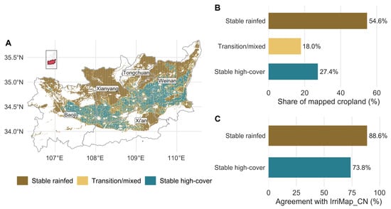
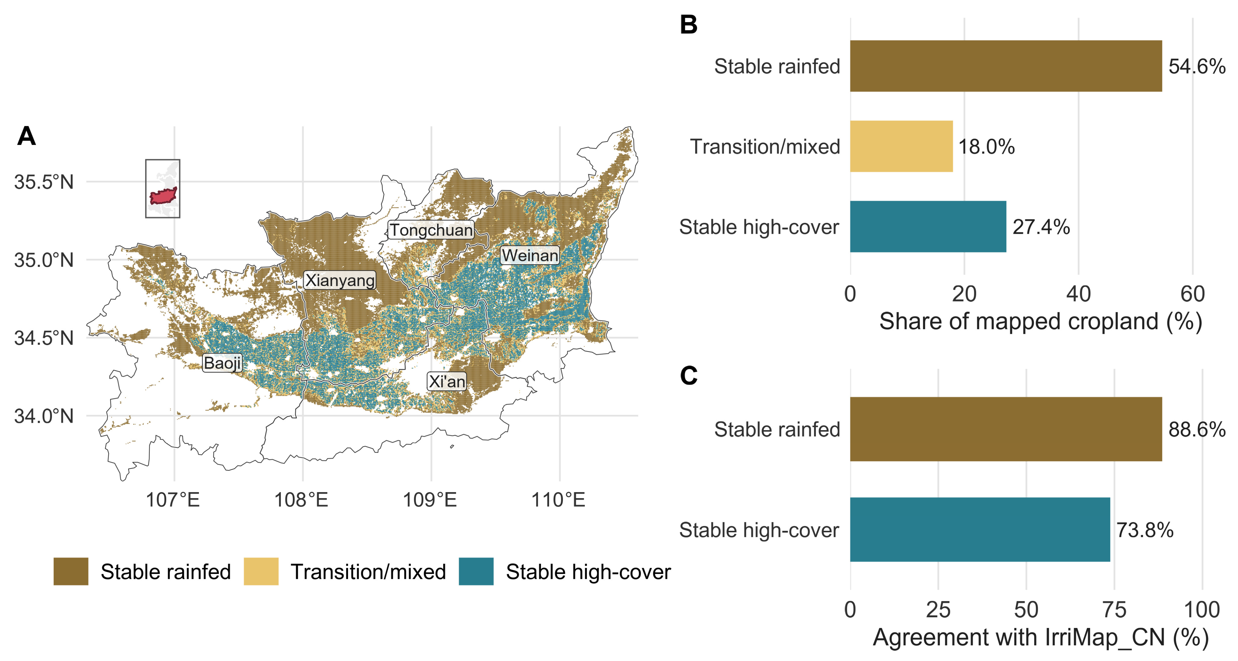
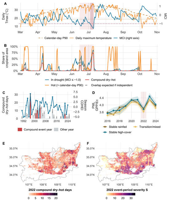
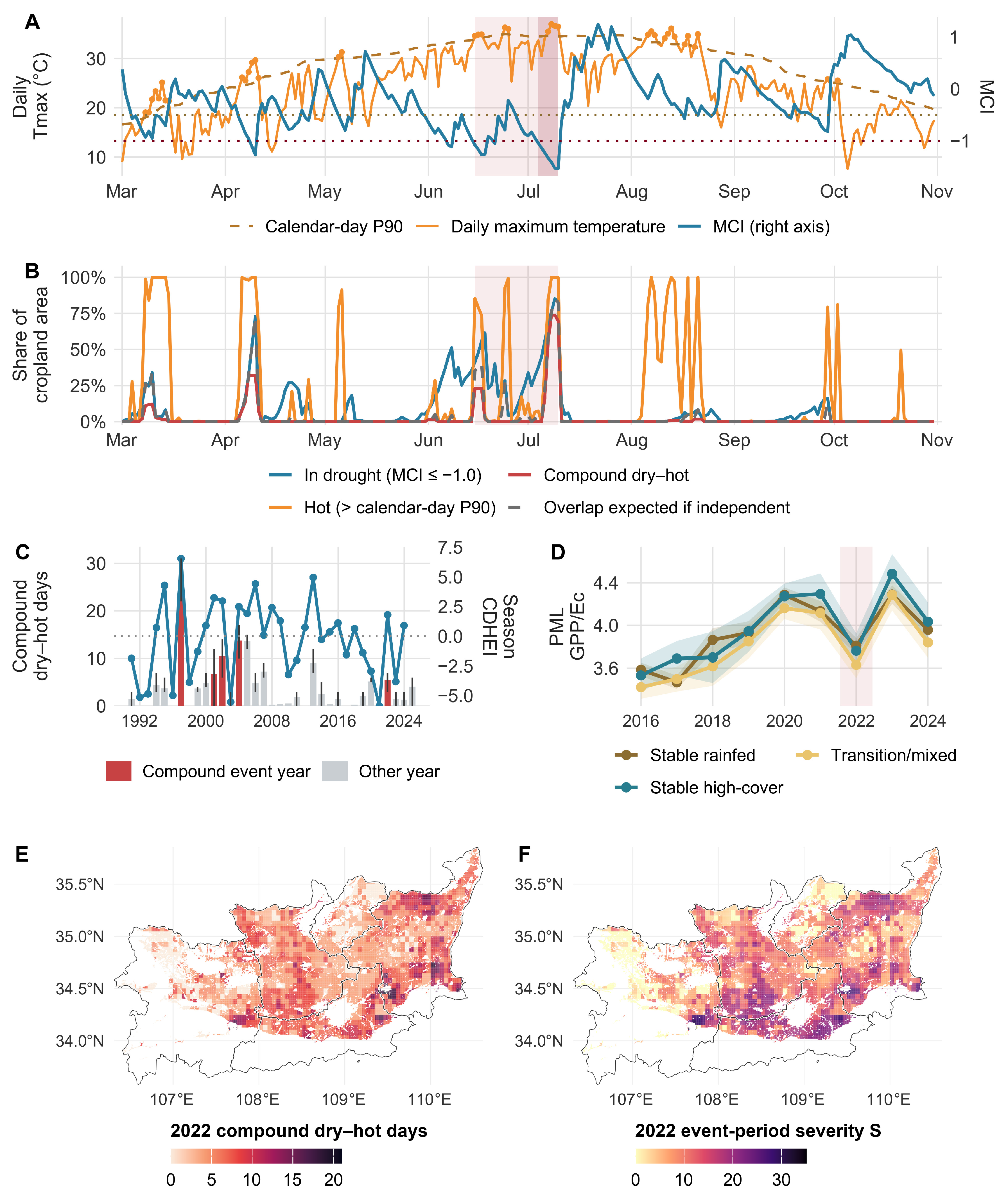
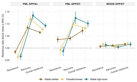
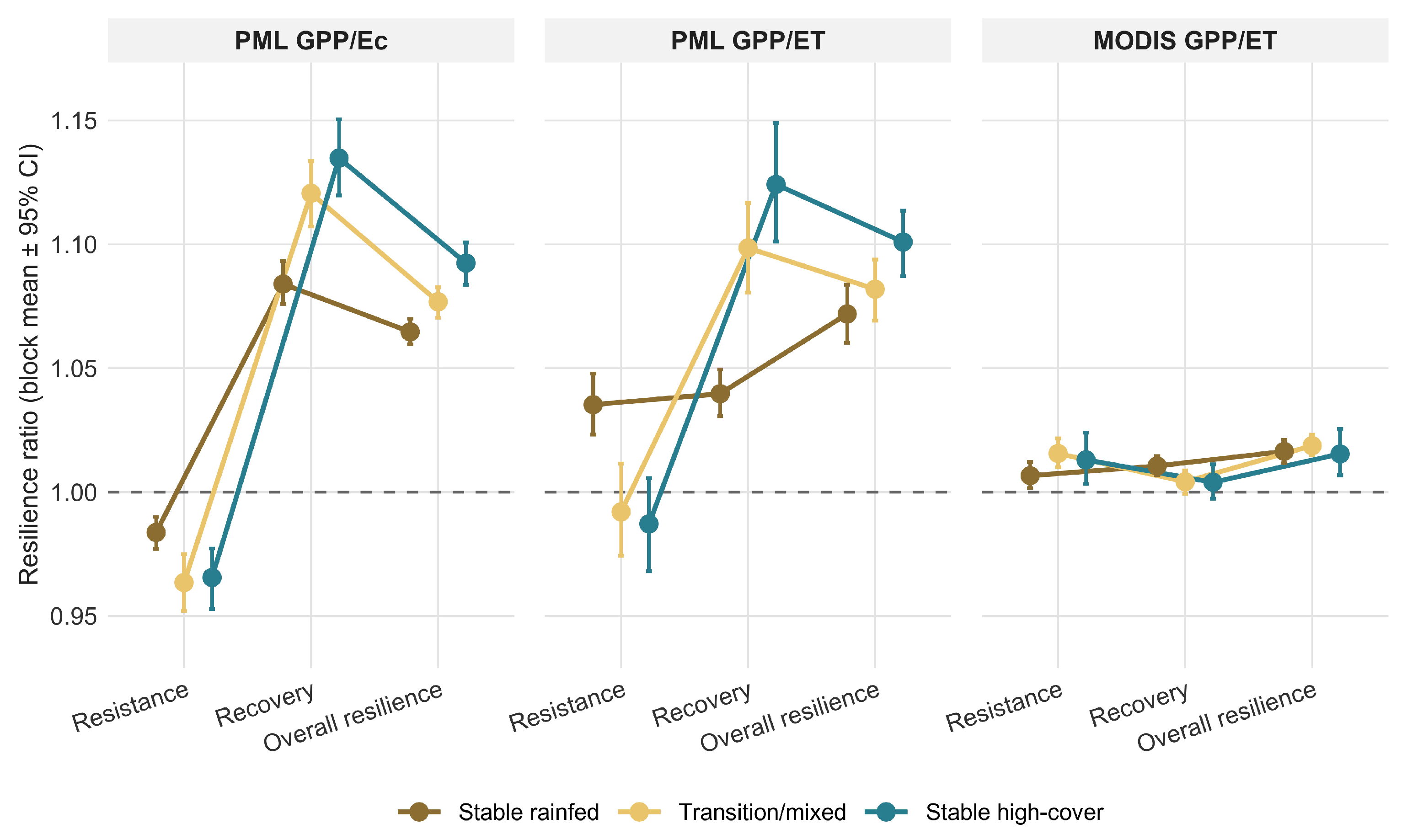
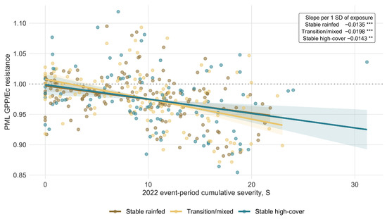
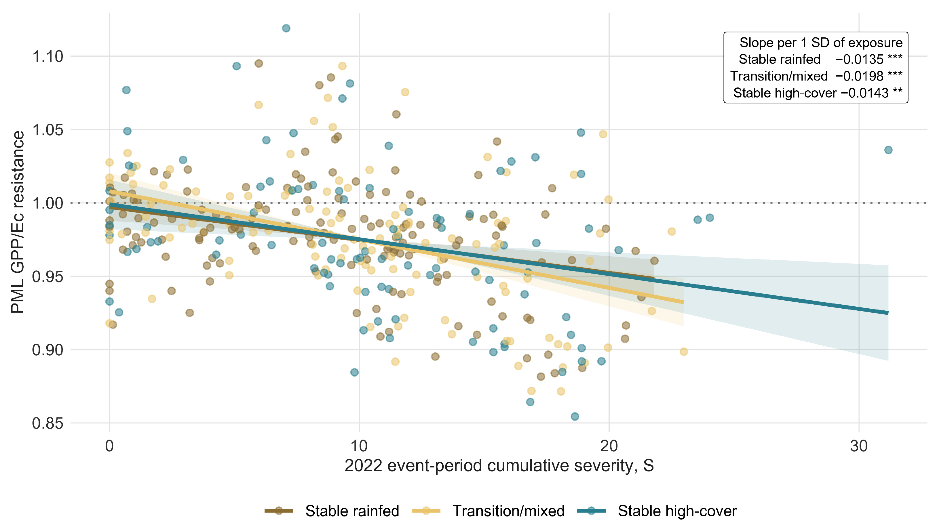
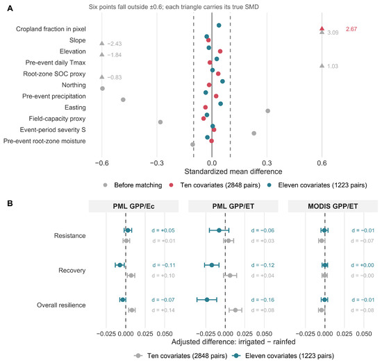
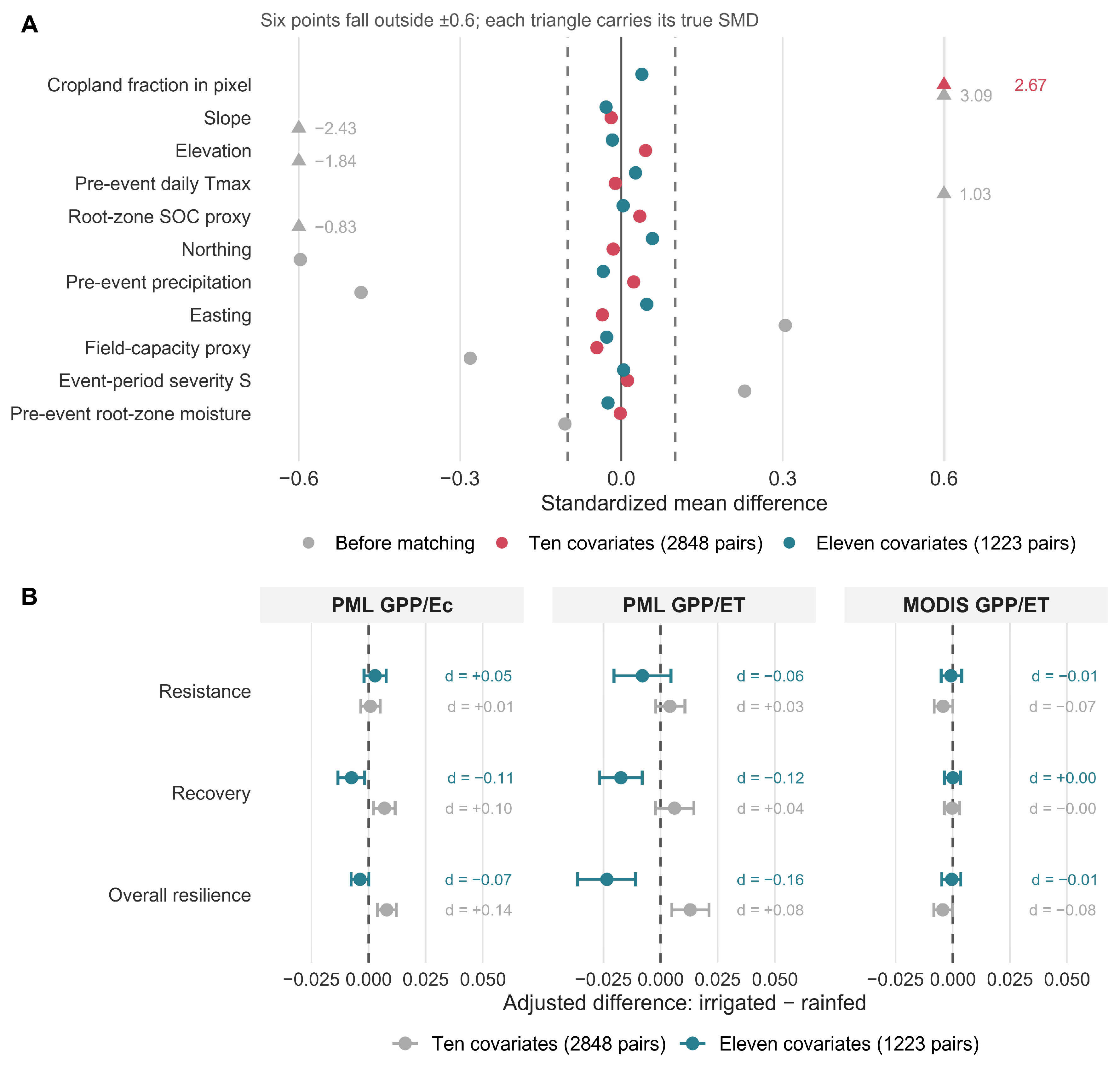
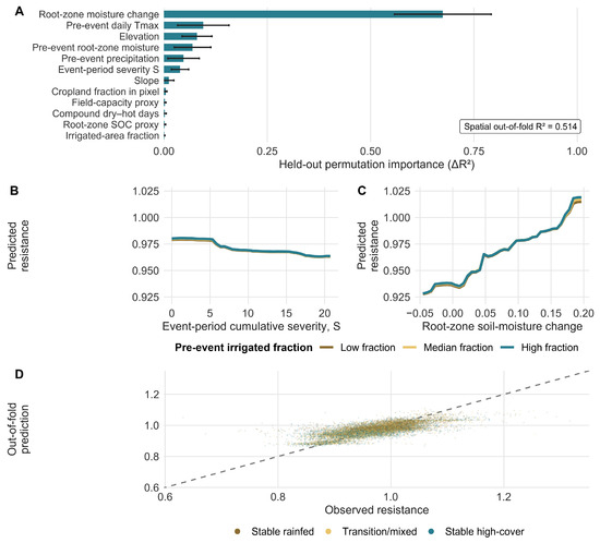
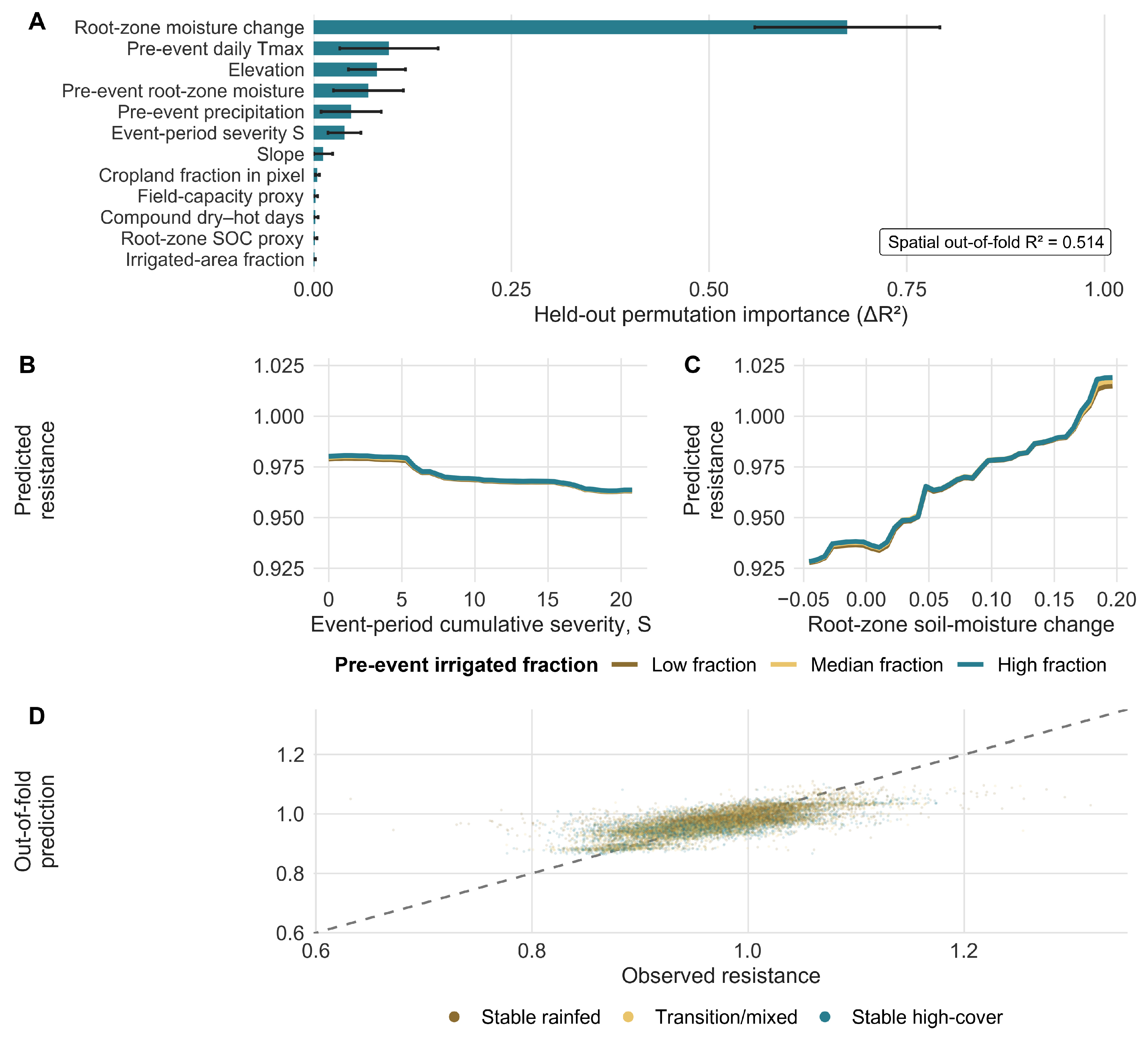
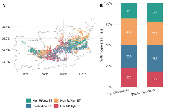
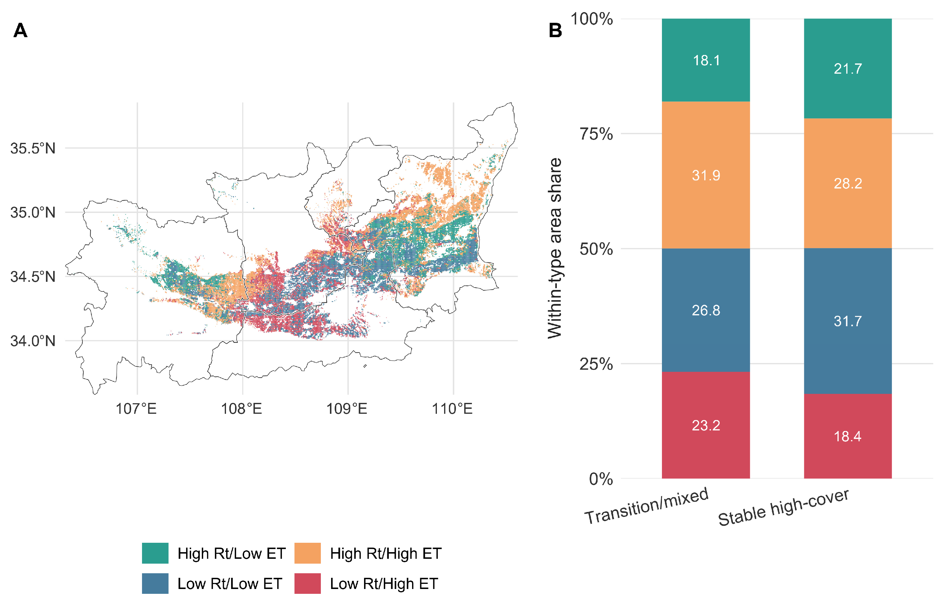
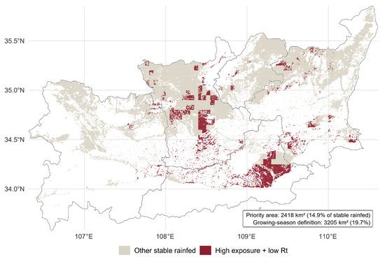
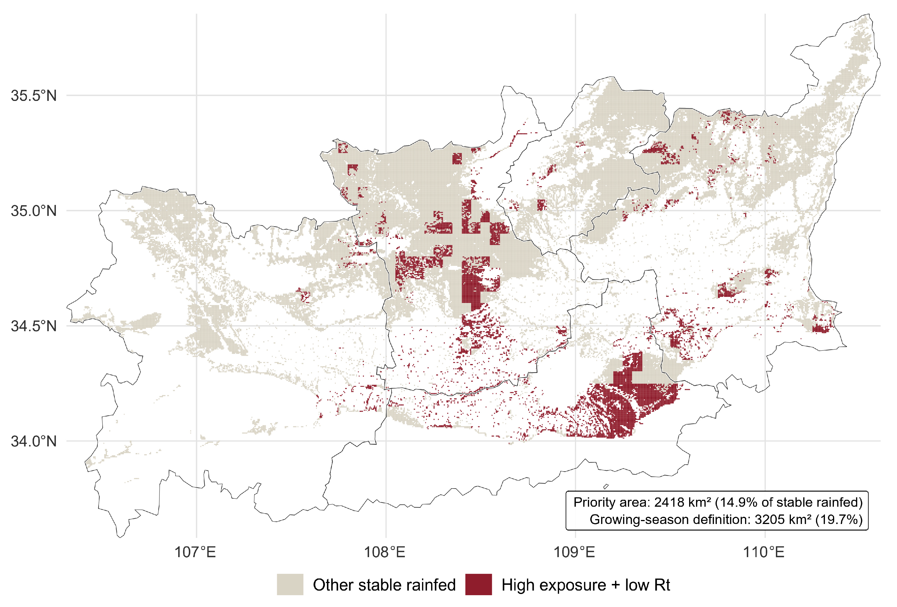
Disclaimer/Publisher’s Note: The statements, opinions and data contained in all publications are solely those of the individual author(s) and contributor(s) and not of MDPI and/or the editor(s). MDPI and/or the editor(s) disclaim responsibility for any injury to people or property resulting from any ideas, methods, instructions or products referred to in the content.

Article Metrics

Citations

Article Access Statistics

Journal Statistics

Multiple requests from the same IP address are counted as one view.

Dataset and Collection Identifier	Native Resolution and Frequency	Period Used	Variables	Quality Control	Temporal Processing	Resampling to 500 m	Use
MODIS land cover MCD12Q1, MODIS/061/MCD12Q1, C6.1 [26,27]	500 m, annual	2016–2020	LC_Type1	No quality-control band; five-year mode; only classes 12 and 14 retained	Pre-event multi-year mode	Native 500 m, nearest neighbor	Cropland mask
CIrrMap250 annual irrigated-cropland maps of China, v1.0 [16]	250 m, annual	2016–2020	Annual irrigated-area fraction	Product no-data values retained	Pre-event five-year mean and persistence	Area-weighted mean	Primary criterion for the irrigation classification
IrriMap_CN annual irrigation maps of China, v1.0 [17]	500 m, annual	2016–2019	Binary irrigation class	Zero values treated as a valid class	Pre-event multi-year irrigation frequency	Area-weighted mean	Independent verification of the classification; core sample
PML-V2.2a evapotranspiration and gross primary productivity, PML/OUTPUT/PML_V22a [22,29]	500 m, 8-day	2016–2024 growing seasons	GPP, ET, Ec	No quality-control band	Growing-season mean of the 8-day composites, then the multi-year mean for each of the three periods	Native 500 m	Primary carbon and water fluxes; both definitions of carbon–water productivity
MODIS gross primary productivity MOD17A2HGF, MODIS/061/MOD17A2HGF, C6.1 [30]	500 m, 8-day, gap-filled	2016–2024 growing seasons	Gpp, Psn_QC	Gpp < 32,760 and the lowest bit of Psn_QC equal to 0	Growing-season sum of the composites	Native 500 m	Independent GPP
MODIS evapotranspiration MOD16A2GF, MODIS/061/MOD16A2GF, C6.1 [23,31]	500 m, 8-day, gap-filled	2016–2024 growing seasons	ET, ET_QC	ET < 32,760 and the lowest bit of ET_QC equal to 0	Growing-season sum of the composites	Native 500 m	Independent ET
MODIS vegetation indices MOD13A1, MODIS/061/MOD13A1, C6.1 [35]	500 m, 16-day	2016–2024 growing seasons	NDVI, SummaryQA	SummaryQA ≤ 1 and NDVI within [−2000, 10,000]	Growing-season mean of the composites	Native 500 m	Vegetation-state reference
ERA5-Land daily aggregates, ECMWF/ERA5_LAND/DAILY_AGGR, v1.0.0 [32]	0.1° (≈9 km), daily	June 1990 to 2025; climatology 1991–2020	Maximum and mean air temperature, dewpoint temperature, three soil-moisture layers	Reanalysis product, no QC band; temperature converted from kelvin by subtracting 273.15	Daily values used for the drought index, the heat threshold, and event-period exposure; growing-season means used for the pixel-level variables; soil moisture weighted by depths of 0.07, 0.21, and 0.72 m	Detection completed on the 0.05° grid and then replicated from the parent cell; root-zone soil moisture and air temperature replicated from the native 0.1° parent cell to 500 m; no downscaling at any stage	Heat criterion, vapor pressure deficit, root-zone soil moisture
CHIRPS daily precipitation, UCSB-CHG/CHIRPS/DAILY, v2.0 [33]	0.05° (≈5.6 km), daily	June 1990 to 2025	Precipitation	No QC band	Accumulated over 30-day, 90-day, and 150-day windows; recent precipitation weighted within a 60-day window using a daily decay coefficient of 0.85; also accumulated over the growing season	Detection on the native 0.05° grid, then parent-cell replication	Drought-index components and precipitation anomaly
TerraClimate monthly climate and water balance, IDAHO_EPSCOR/TERRACLIMATE [34]	1/24° (≈4.6 km), monthly	1991–2024 growing seasons	Reference evapotranspiration, ASCE Penman–Monteith method	No quality-control band	Monthly values summed over the growing season	Upsampled by parent-cell replication	PET term of the growing-season exposure index
OpenLandMap water content at 33 kPa, SOL_WATERCONTENT-33KPA_USDA-4B1C_M, v01 [36]	250 m, static	Static	Volumetric water content, bands b0–b100	No quality-control band	Depth-weighted over 0–100 cm with weights of 0.05, 0.15, 0.25, 0.35, and 0.20	Pyramid mean	Field-capacity proxy
OpenLandMap soil organic carbon, SOL_ORGANIC-CARBON_USDA-6A1C_M, v02 [37]	250 m, static	Static	Bands b0–b100, values expressed in multiples of 5 g kg⁻¹	No quality-control band	Depth weighting as above; used as a relative covariate	Pyramid mean	Root-zone soil organic carbon proxy
SRTM digital elevation model, USGS/SRTMGL1_003 [38]	30 m, static	Static	Elevation, slope	No quality-control band	Slope derived on the native grid before aggregation	Area-weighted aggregation	Terrain covariates
ESA WorldCover, ESA/WorldCover/v200 for 2021, with v100 for 2020 used for cross-checking [28]	10 m, single epoch	2021 and 2020	Map; class 40 is cropland	Binary mask aggregated and then restricted to the cropland mask	Single epoch, converted to an areal fraction	Areal fraction on the analysis grid	Subpixel cropland fraction

Class	CIrrMap250 Criterion, 2016–2020	IrriMap_CN Independent Verification Criterion, 2016–2019	Agreement (%)	Mapped Area (km²)	Share of Mapped Cropland (%)	Role in the Analysis
Stable rainfed	Five-year mean irrigated-area fraction ≤ 20% and persistence ≤ 0.2	Irrigation frequency ≤ 0.25 counted as agreement	88.6	16,340.6	54.6	Control group in the binary comparison; exposure–response relationship; regional screening zonation
Transitional/mixed irrigation	All remaining cropland that reaches neither stable end member	No hard criterion	—	5384.0	18.0	Exposure–response relationship; regional screening zonation
Stable high-coverage irrigation	Five-year mean irrigated-area fraction ≥ 60% and persistence ≥ 0.8	Irrigation frequency ≥ 0.75 counted as agreement	73.8	8179.4	27.4	Treatment group in the binary comparison; exposure–response relationship; regional screening zonation

Identification Step	Value
Number of detection cells, and the number of those overlying cropland	4089 and 1700
Share of the cropland area with at least one compound dry–hot day	88.9%
Mean, median, and maximum number of compound dry–hot days over cropland	5.47, 5, and 21 days
Mean number of days at moderate drought grade or worse per cell	21.6 days
Mean number of hot days per cell	40.2 days
Observed and independence-expected dry–hot overlap	8.5 and 3.5 days
Median ratio of observed to expected overlap, and share of cells with a ratio above one	2.53 and 98.8%
Peak share of compound cells, and the date on which it occurred	73.8% on 8 July
Cropland-area-weighted median compound dry–hot window	15 June to 10 July
Regional core event window	4 July to 10 July
Mean, median, and maximum event-period cumulative severity S over cropland	10.34, 10.11, and 35.14
Share of pixels with no compound dry–hot day, for which S is zero	11.1%

Zone	Relative Decision Rule	Area (km²)	Share	Mean Resistance	Diagnostic Label
High resistance, low ET response	Resistance ≥ median; response < median	2727.0	20.3%	1.003	Relative benchmark
High resistance, high ET response	Resistance ≥ median; response ≥ median	3986.1	29.6%	1.017	Water-use audit
Low resistance, low ET response	Resistance < median; response < median	3998.4	29.7%	0.915	Resilience improvement
Low resistance, high ET response	Resistance < median; response ≥ median	2736.2	20.3%	0.924	Joint audit

Root-Zone Moisture Realized During a Compound Dry–Hot Event, Not Irrigation Persistence, Determines the Resilience of Cropland Carbon–Water Productivity in the Guanzhong Plain, China

Abstract

1. Introduction

2. Materials and Methods

2.1. Study Area, Analysis Grid, and Multi-Source Observations

2.2. Pre-Event Irrigation Classes and Definition of the Treatment Variable

2.3. Pixel-Wise Identification of the Compound Drought–Heat Event and Quantification of Exposure

2.4. Carbon–Water Productivity and the Three-Component Resilience Framework

2.5. Statistical Inference, Mechanistic Evaluation, and Regional Screening Zonation

3. Results

3.1. The Three Cropland Classes Cover 29,904.0 km2, and 88.9% of That Area Experienced Concurrent Drought and Heat in 2022

3.2. Irrigation Persistence Confers No Carbon–Water Productivity Advantage Either During or After the Event

3.3. The Cost of the Event Was a Decline in Water-Use Efficiency Rather than a Loss of Carbon Assimilation

3.4. The Spatial Pattern of Resistance Is Explained Mainly by the Root-Zone Moisture Status Realized During the Event

3.5. Water-Use Audit Zones Cover 6722.3 km2 of Irrigation-Related Cropland, and 2418.1 km2 of Rainfed Cropland Forms a High-Exposure, Low-Resistance Priority Zone

4. Discussion

4.1. Irrigation Persistence Did Not Raise Event-Year Resistance, and the Apparent Post-Event Recovery Advantage Originates in Subpixel Cropland Composition

4.2. Event-Period Moisture Status, Rather than Irrigation Status Itself, Explains the Spatial Variation in Resistance

4.3. Allocating Limited Water Around the Moisture Status Realized During the Event

4.4. Limitations and Directions for Further Verification

5. Conclusions

Supplementary Materials

Author Contributions

Funding

Data Availability Statement

Conflicts of Interest

Abbreviations

References

Article Metrics

Article Access Statistics

3.1. The Three Cropland Classes Cover 29,904.0 km², and 88.9% of That Area Experienced Concurrent Drought and Heat in 2022

3.5. Water-Use Audit Zones Cover 6722.3 km² of Irrigation-Related Cropland, and 2418.1 km² of Rainfed Cropland Forms a High-Exposure, Low-Resistance Priority Zone