


Abstract
In mountainous river basins, groundwater systems are sustained by complex recharge processes and geological heterogeneity, making groundwater flow simulation challenging in data-scarce regions where hydrological inputs are often assumed to be spatially uniform. This study developed a heterogeneous geological model of the Kofu Basin, Japan, using multiple boreholes and simulated the groundwater flow by integrating MODFLOW with climate-driven recharge outputs from SWAT+. Simulated groundwater flow was evaluated against findings from previous stable isotope studies to assess the plausibility of the simulated recharge system. After calibration, the model performance improved substantially: RMSE decreased by 91.28%, MAE decreased by 84.38%, and NSE increased from 0.9530 to 0.9996. Independent validation showed good regional agreement between observed and simulated groundwater heads (R2 = 0.9307; NSE = 0.9254), although RMSE and MAE remained relatively high at 32.70 m and 19.76 m, respectively, suggesting remaining uncertainty in local-scale groundwater head simulation. Simulated velocity vectors indicated localized shallow flow and more coherent regional basinward flow in the deeper aquifer. This pattern is consistent with the interpretation that mountain-derived recharge contributes to the deeper regional groundwater system. The results highlight the value of combining hydrogeological models and geochemical evidence to support recharge-process interpretation in complex mountainous basins.
1. Introduction
1.1. Background
Mountainous river basins are vital hydrological systems that play a critical role in global water distribution [1,2]. They provide substantial water resources to downstream regions through precipitation and snowmelt, which are subsequently transferred through surface runoff and groundwater flow. This distribution supports agriculture, hydropower, and domestic water supply far beyond the mountain boundaries.
Groundwater is an integral component of the hydrologic cycle [3,4,5]; however, increasing water demand and climate variability threaten its sustainability [6]. Consequently, computer models have become indispensable tools for predicting groundwater dynamics. Many studies have simulated independent groundwater flow [7,8] and the interaction between surface water and groundwater [9,10,11].
Groundwater modeling has been widely recognized in the fields of hydrology and water resource management for its ability to describe aquifer characteristics and forecast the status of groundwater storage and use [12,13,14,15]. Such models provide insights into the operation of hydrological systems under the influence of climate conditions, precipitation, groundwater recharge, and groundwater use [12,16,17]. The MODFLOW model enables three-dimensional (3D) groundwater modeling using the finite-difference method. This model can be applied to mountainous terrains, heterogeneous aquifer formations, and localized recharge zones [18,19]. This study employs MODFLOW-NWT, a Newton formulation for MODFLOW-2005 with upstream weighting to improve the numerical treatment of nonlinearities associated with unconfined flow and cell drying/rewetting, thereby enhancing convergence stability compared with the standard MODFLOW formulation [20].
In data-scarce regions, some initial input data for groundwater modeling are commonly estimated from local conditions, and some parameters, such as evapotranspiration (ET) or recharge rate, are considered homogeneous [21,22]. However, the groundwater system in a mountain area is highly heterogeneous and controlled by elevation, soil properties, and geological structure. As a consequence, the groundwater flow model using spatially uniform input may misrepresent recharge zones and lead to uncertainty in simulated hydraulic heads and flow paths. The Kofu Basin in Yamanashi Prefecture is a distinctive mountainous catchment in Japan. The area is characterized by steep mountainous topography and extensive forest cover. In some remote areas, particularly headwater areas, monitoring networks are unavailable or discontinuous. Additionally, the monitoring system in the Kofu Basin is not very dense; most of the observations are located in residential areas and along the main river.
According to previous integrated SWAT–groundwater studies, distributed recharge estimates can improve groundwater conceptualization [23,24,25]. Groundwater flow models are commonly evaluated mainly through hydraulic head calibration, while independent geological and geochemical evidence is less frequently integrated into model validation. This creates uncertainty in interpreting recharge processes, especially in the basins where mountain block recharge (MBR), mountain front recharge (MFR), and local precipitation recharge may interact. To reduce modeling uncertainty, the groundwater flow model uses hydrological simulation outputs driven by climatic data as initial conditions. In addition, the simulated mountain recharge zones are evaluated based on evidence from earlier isotope-based investigations in the Kofu Basin [26], which identified the contribution of mountain recharge and demonstrated its spatial variability. An approach that integrates hydrological modeling, geological knowledge, and spatially distributed recharge was developed to improve the accuracy of groundwater flow simulation. This method provides a realistic representation of groundwater dynamics in the Kofu Basin and provides a more constrained basis for interpreting recharge processes and regional groundwater flow patterns in a complex mountainous basin. This approach supports informed decision-making for groundwater allocation, forest management, and climate adaptation, ensuring that ecological and human water demands are met.
1.2. Study Area
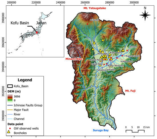
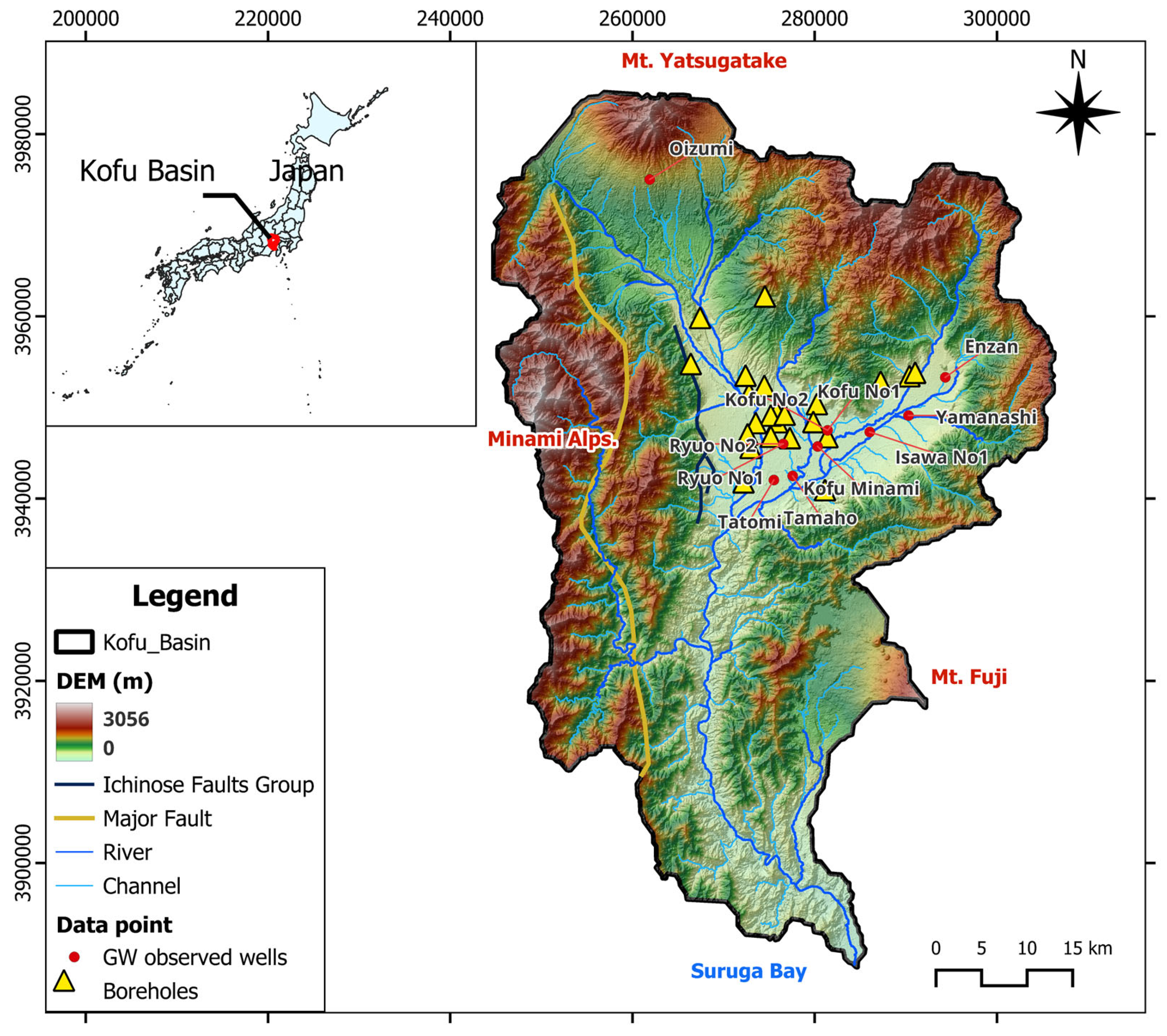
The Kofu Basin, situated in Yamanashi, Japan, is surrounded by steep mountains that reach approximately 2000 m above sea level, including Yatsugatake Mountain, Mount Fuji, Kinpu Mountain, and the Minami Alps (Figure 1). The Kofu Basin is formed by two large alluvial fans, the Kamanashi and Fuefuki Rivers, where the river beds are elevated due to sediment deposition. These alluvial fans create highly permeable aquifers that serve as critical groundwater reservoirs, providing a stable water supply that complements surface streamflow. These aquifers provide groundwater that is extensively used for domestic consumption, agriculture, and industry, highlighting the strong link between the basin hydrogeology and regional socioeconomic activities.
Figure 1.
Study area of the Kofu Basin showing topography, basin boundary, river network (light blue lines), fault distribution (dark blue and yellow lines), groundwater observation wells (red dots), and borehole locations (yellow triangles).
The basin displays a mixed land cover, with dense forests in the uplands and intensive agriculture and urban development in the lowlands. This heterogeneous land cover influences basin hydrology in terms of infiltration, ET, and groundwater recharge. Beyond its natural characteristics, the Kofu Basin is one of Japan’s primary agricultural and residential regions. Vineyards, orchards, and rice paddies throughout the basin rely on a combination of river water and groundwater, and urban centers rely on stable aquifer recharge to meet their domestic water demands.
The Kofu Basin lies within the South Fossa Magna, where volcanic arcs and crustal blocks have collided and been uplifted [27]. The mountainous blocks around the basin comprise granitoids, volcanic rocks, and metamorphic complexes. The basin floor is filled with thick Quaternary alluvial and fluvial deposits [28]. The flat area of the basin comprises alluvial fans formed by several rivers, most of which are tributaries of the Kamanashi, Fuefuki, and Midai Rivers. The typical stratigraphy beneath the flat lowland area comprises coarse gravel and fine sand, which are locally interbedded with volcanic ash and clay. The top layer acts as an unconfined aquifer with high hydraulic conductivity and connects to the rivers, whereas local finer and impermeable units form aquitards that separate shallow groundwater systems from deeper groundwater systems.
2. Materials and Methods
2.1. 3D Geological Model
2.1.1. Borehole Data
As fundamental input for geological models, borehole data provide direct and reliable information on the vertical distribution of subsurface materials. These data enable delineation of lithostratigraphic boundaries and identification of aquifer and aquitard layers.
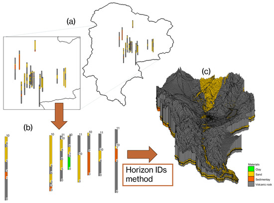
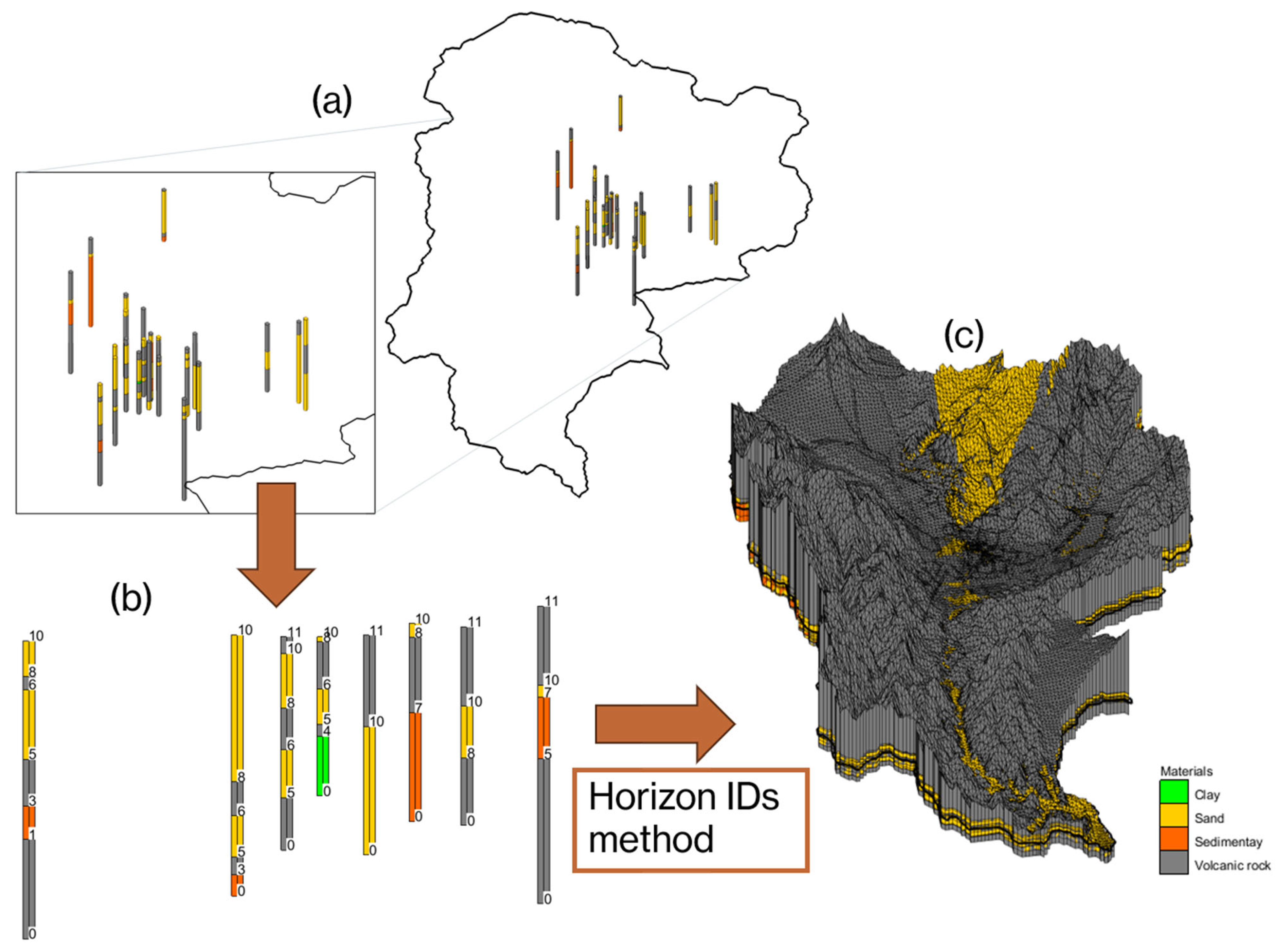
Figure 2a shows the spatial distribution of 22 borehole geological profiles used to construct the 3D geological model of the Kofu Basin developed using the groundwater modeling system (GMS v10.8). Each vertical column represents an individual borehole log, with color segments denoting the identified lithological units: clay (green), sand (yellow), sedimentary rock (orange), and volcanic rock (gray). Most of the borehole logs are located in the central basin area.
Figure 2.
Procedure for 3D geological model development in the Kofu Basin. Spatial distribution of geological boreholes within the basin. (a) Spatial distribution of borehole lithological logs within the basin. (b) Horizontal view of geological boreholes with horizon IDs. (c) Reconstructed 3D geological model generated using the horizon ID method, showing the spatial distribution of major subsurface materials, including clay, sand, sedimentary deposits, and volcanic rock.
The horizontal view of geological boreholes reveals that the subsurface is dominated by alternating layers of sand, gravel, and volcanic rock, interbedded with minor silt and clay (Figure 2b). The stratigraphic configuration indicates the presence of shallow unconfined aquifers, whereas finer-grained layers may restrict vertical groundwater movement and create semi-confined conditions at depth. Sand and gravel layers serve as primary water-bearing formations with high permeability, thereby facilitating lateral groundwater flow and rapid recharge.
2.1.2. Horizon IDs to Solid Material
The Horizon ID method, introduced by Wang et al. [15] was applied to define and correlate the subsurface stratigraphic boundaries among the boreholes. This method has proven effective for reconstructing geological systems when sufficient borehole data are available. The horizon IDs method consists of four main steps. In the first step, the “Auto-Create Blank Cross-Section” tool was used to automatically generate blank cross-sections between neighboring boreholes. In the second step, the “Auto-Assign Horizons” tool was used to assign horizon IDs to borehole contacts based on material ordering and adjacent boreholes. In the third step, the previously generated blank cross sections were filled by connecting the contacts on one borehole to those on the other using the “Auto-Fill Blank Cross-Section” tool. Finally, in the fourth step, the completed cross sections were converted into solids using the “Horizons → Solids” function to construct the 3D geological model. The 3D model is able to show the distribution of the subsurface formations. Volcanic rock predominates in the deeper sections and along the basin borders, whereas sand and gravel dominate the central and lower basin, corresponding to the Kamanashi and Fuefuki alluvial fans.
From the geological solids, the GMS can be converted to a grid-based model, thus enabling the execution of the MODFLOW model (Figure 2c). This conversion assigns each cell of the MODFLOW grid the lithological and hydraulic properties defined in the geological model. The model uses a 3D grid covering a cell size of 500 × 500 m and 15 layers, which is suitable for the study area and the available hardware capacity.
2.2. Groundwater Flow Model
2.2.1. Model Structure and Domain
A 3D steady-state groundwater flow model was developed to represent the basin-scale hydrological system in the Kofu Basin using MODFLOW-NWT within the GMS v10.8. The steady-state assumption was selected because the main objective was to evaluate regional hydraulic gradients and potential recharge pathways rather than seasonal groundwater level fluctuations. In addition, available observations were not sufficient to calibrate a transient model, and spatially distributed continuous monitoring data were limited.
The model domain was defined to include the alluvial basin and adjacent mountainous recharge areas, allowing the representation of local and regional groundwater flows. The model’s spatial extent (mostly mountainous area) and vertical layering were based on the 3D geological framework, based on the borehole lithology, geological knowledge, and topographic information.
The hydrogeological system is vertically discretized into two main aquifers: (1) the shallow unconfined aquifer, composed mainly of coarse sand and gravel alluvial fan deposits, and (2) the deep semi-confined aquifer, composed of compacted sand, tuff, and fractured volcanic formations.
2.2.2. Governing Equation
The groundwater flow in the model is governed by the 3D Darcy’s steady-state condition implemented in MODFLOW [29]:
where represents the hydraulic head (L), , , and denote the hydraulic conductivity in , , and directions (LT−1), respectively, and represents the volumetric flux per unit volume representing sources and sinks, such as recharge, ET, river leakage, or pumping (T−1).
2.2.3. Boundary Conditions
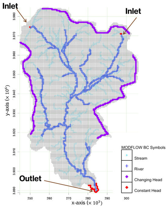
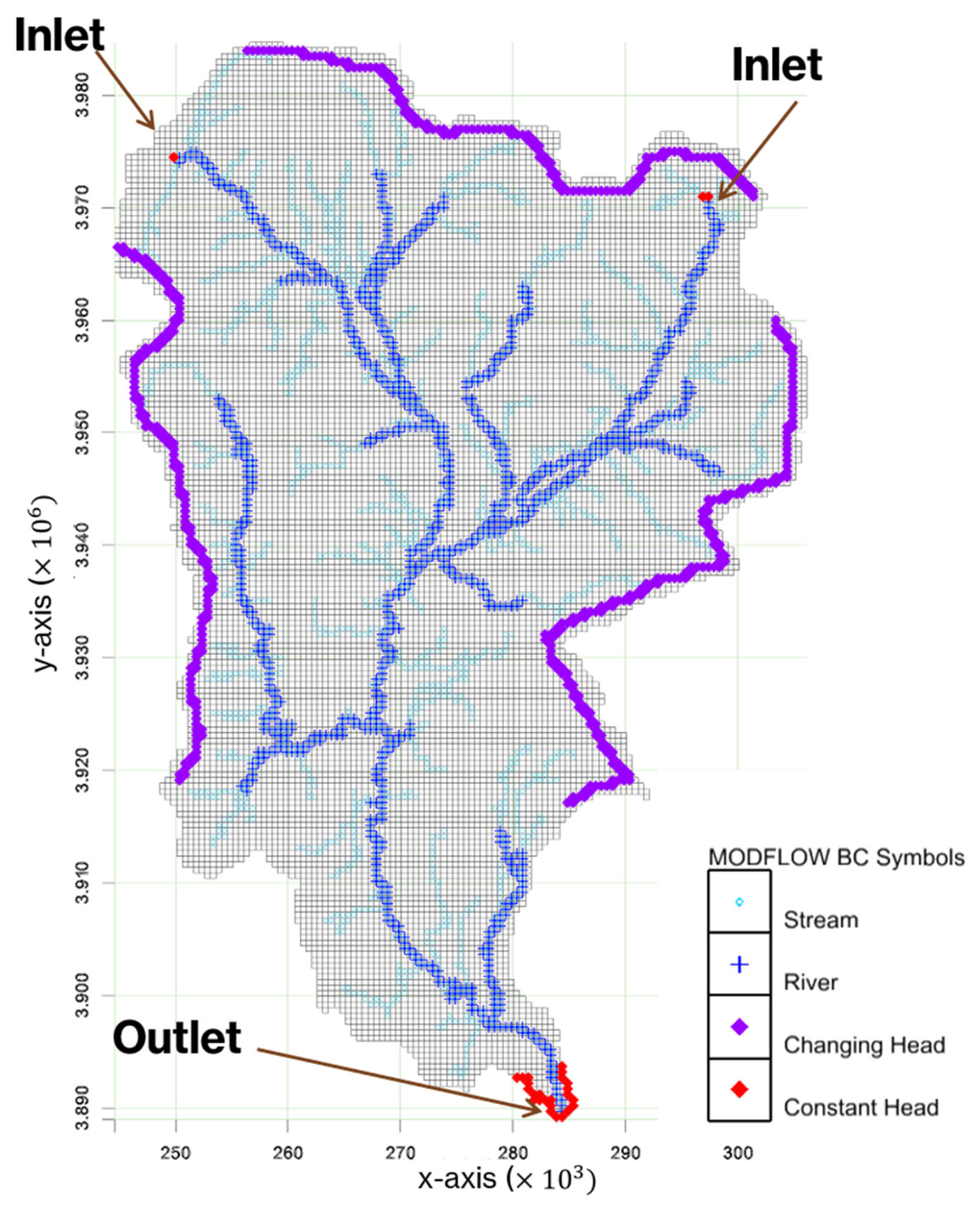
The boundary conditions of the 3D model were assigned based on the regional hydrogeological setting of the Kofu Basin. These conditions are shown in Figure 3, which presents the spatial configuration of the hydrological boundary conditions used in the MODFLOW groundwater flow model. Specified head boundaries were used only where external hydraulic control was necessary to reproduce the regional flow conditions.
Figure 3.
Boundary condition of the 3D model. Two inlets and one outlet area are represented by red diamonds; the changing head boundary is represented by violet diamonds; streams are represented by light blue dots, and rivers are represented by blue crosses.
The two inlet boundaries (north and northwest) represent the groundwater inflow zones corresponding to the river upstream. These boundaries are set as constant head cells using the Specified Head package (CHD) to maintain stable hydraulic heads in the basin. The outlet boundary is located in the southern part of the basin and was treated as a downgradient groundwater outflow boundary. These cells were assigned constant-head boundary conditions to simulate regional groundwater discharge.
The packages used in the model are listed in Table 1. The Upstream Weighting package, which is suitable for heterogeneous catchment materials, was used to compute cell-by-cell hydraulic conductance. The Newton solver can handle nonlinearities in unconfined groundwater flow equations, ensuring convergence even under dry or rewetting conditions. The Evapotranspiration and Recharge packages help input the climate value, which has been simulated in previous works. The river network is represented using the River and Stream packages. These packages simulate surface–groundwater interactions, allowing groundwater to discharge into rivers and receive recharge from local head gradients.
Table 1.
Details of MODFLOW packages used in the 3D groundwater flow model.
2.2.4. Hydraulic Properties
Hydraulic properties were assigned according to the interpreted geological units, and Table 2 summarizes them for each material in the 3D model. The parameters include horizontal hydraulic conductivity (Kh), vertical anisotropy ratio (Kh/Kv), specific storage, specific yield, and porosity. Because of a lack of field experiments and resources, these values were selected based on the studies by Khan et al. [30], and Earle [31]. Sand and gravel exhibit high hydraulic conductivities and specific yields, reflecting the primary groundwater aquifer layers. Volcanic rock exhibits intermediate hydraulic conductivity due to its fractures. In contrast, fine-grained materials, such as clay and silt, exhibit extremely low conductivities and act as a barrier, restricting groundwater flow in the model. Sedimentary rocks exhibit the lowest conductivity due to their compacted characteristics. Initially, spatially uniform recharge and ET rates were assigned for the steady-state simulation, with the recharge and ET rates set to 0.0005 and 0.001 m/d, respectively. Subsequently, the model used the recharge and ET values from the QSWAT+ model to assess the potential of the adaptation data for the groundwater model.
Table 2.
Initial condition of the 3D groundwater flow model [30,31].
2.2.5. Adaptation Data from SWAT+ Model
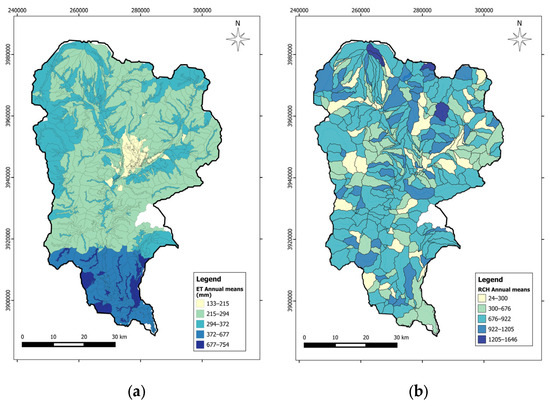
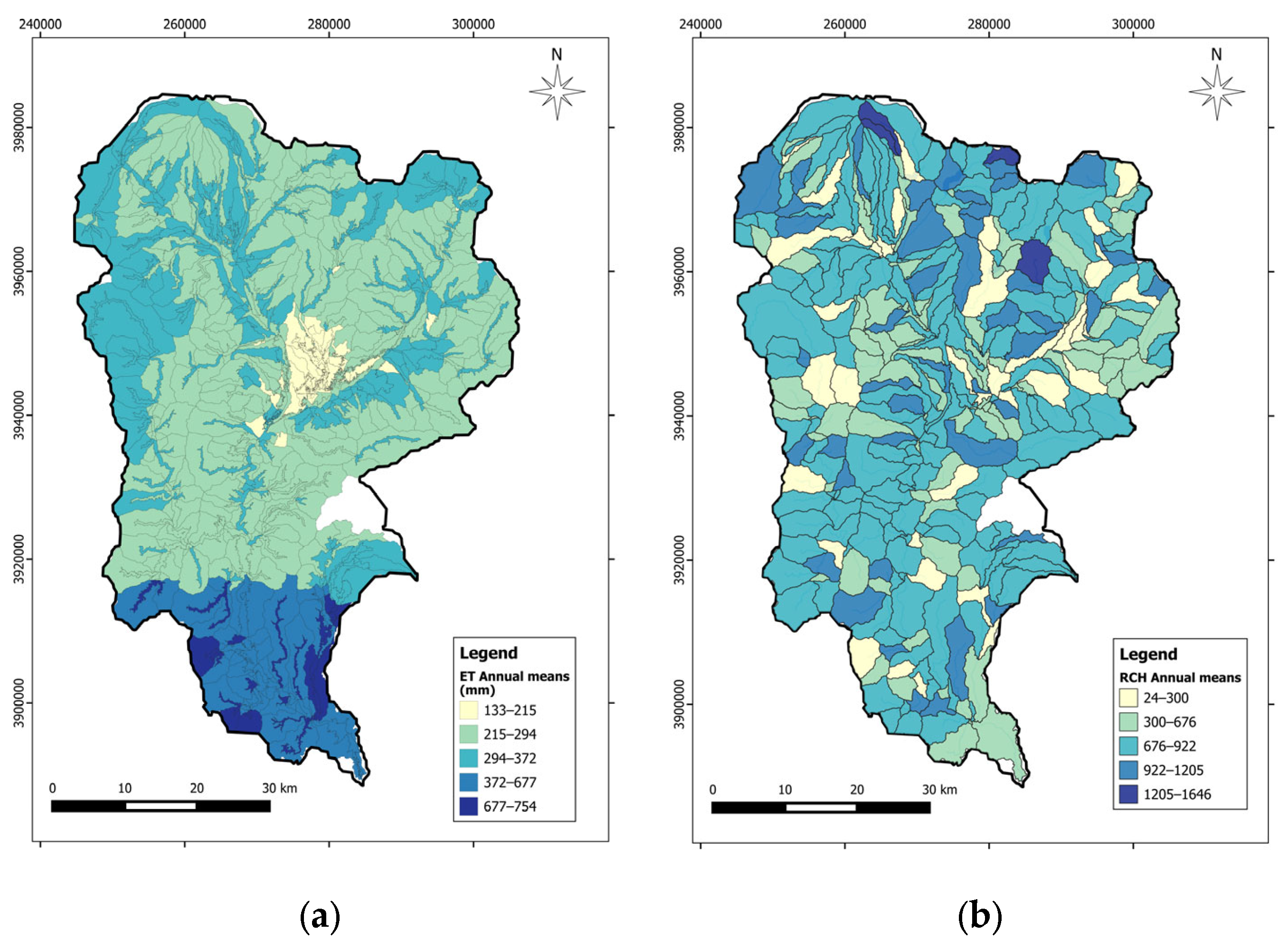
Figure 4a,b present the spatial distribution of ET and groundwater recharge, which serve as input data for the MODFLOW model. The ET and recharge fields were derived from a previously developed SWAT+ watershed model for the Kofu Basin, whereas the groundwater table elevations were interpolated from local domestic groundwater well measurements. Typically, groundwater studies conducted in data-scarce regions assume recharge to be spatially uniform or indirectly estimated from limited field observations. However, recharge and evapotranspiration may vary across the basin because of differences in precipitation, elevation, slope, land cover, soil properties, and alluvial-fan characteristics. Groundwater modeling with assigned uniform recharge may oversimplify recharge zones and distort simulated groundwater head and flow pathways. Therefore, climate-driven recharge estimates from hydrological models can provide a more physically meaningful input for basin-scale MODFLOW simulations, especially in regions where direct recharge observations are limited.
Figure 4.
Spatial distribution of (a) annual evapotranspiration (ET), and (b) recharge (RCH) rate.
Figure 4a shows the spatial variation in ET (133–754 mm), which is lower in high elevation areas and higher in the southern lowlands. Figure 4b shows the recharge (24–1646 mm). Spatially distributed recharge from the SWAT+ model was used to assign through the RCH package as diffuse recharge from rainfall infiltration.
The SWAT–MODFLOW often relies on simplified aquifer representation, which is simulated by using land use and soil properties [32,33], and commonly focus on the shallow aquifer. By incorporating borehole-derived geological profiles into an independent groundwater flow model, this approach enables a more realistic representation of deeper aquifer systems.
2.2.6. Model Calibration, Evaluation, and Validation
The groundwater flow model was calibrated against observed groundwater head obtained from monitoring wells distributed across the basin. Twelve observed wells were used for model calibration (Figure 1). Most of the wells are located in the central lowland area of the catchment, with only the Oizumi well located on the foothill of Mt. Yatsugatake. Groundwater heads were monitored daily at the observation wells, and the long-term mean groundwater head at each well was used for model calibration. The details of these wells are presented in Table 3.
Table 3.
Observed wells.
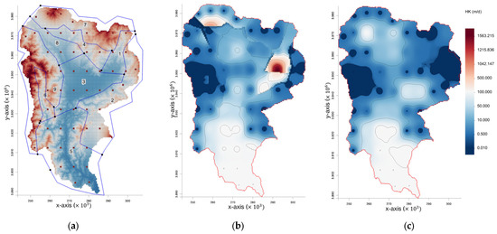
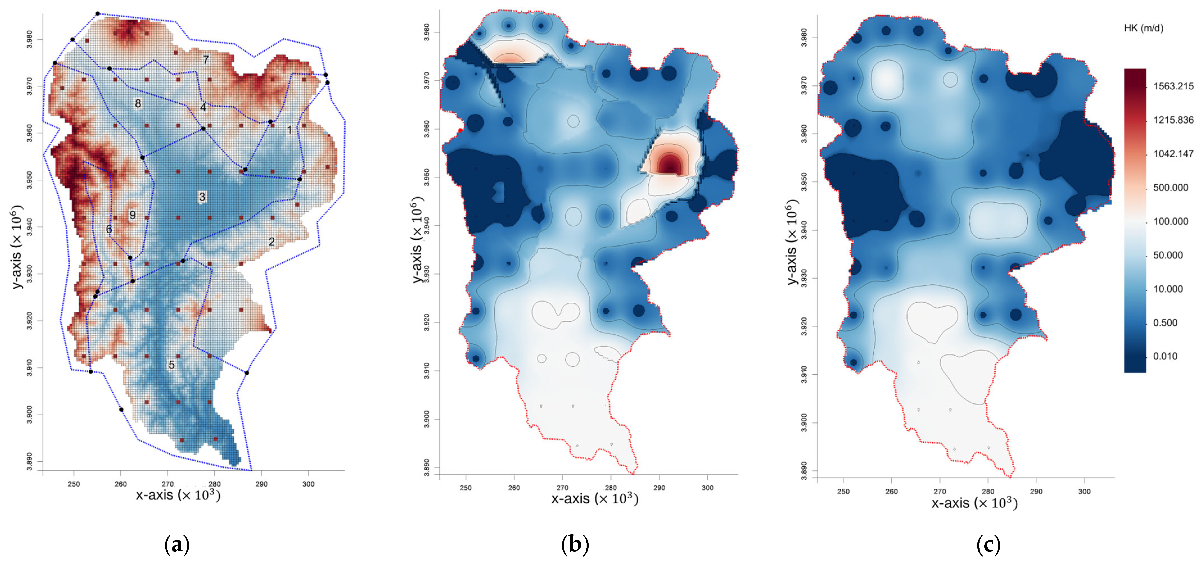
Calibration was performed by adjusting sensitive hydraulic parameters and boundary-condition-related inputs within physically plausible ranges to improve the agreement between simulated and observed groundwater levels. In this case, attention was given to recharge distribution, constant head at the boundary, and hydraulic conductivity contrasts among geological units, since these factors strongly influence groundwater flow in the basin. The hydraulic conductivities in the 3D model are delineated based on geological characteristics. Each zone defines a permissible range of hydraulic conductivity values for pilot points calibration (Figure 6a). The hydraulic conductivities are divided as follows:
- Zones 1, 3, 5, and 8 correspond to the large river alluvial fans, dominated by coarse sand and gravel with high permeability;
- Zones 6 and 9 correspond to the Minami Alps area, which is characterized by a complex sediment–volcanic transition;
- Zones 2, 4, and 7 correspond to the northern and northeastern mountainous areas, primarily composed of rock and granite, and are characterized by low permeability;
The parameter estimation (PEST) algorithm was used for calibration. The following objective function was used in the calibration process:
where and denote the observed and simulated heads at location denotes the weight assigned to each observation, and represents the number of observation points.
The calibrated model was further evaluated using a larger dataset of 298 domestic and geological wells with measured groundwater levels. These wells were not used to adjust model parameters and can serve as independent validation. This additional dataset improves confidence in the basin-scale applicability of the groundwater model.
In addition, the groundwater flow and velocities are simulated and evaluated by comparison with a previous study on mountain recharge in the Kofu Basin. Earlier isotope and hydrochemistry-related results obtained in the Kofu Basin have shown that mountain water considerably contributes to groundwater, especially in the deep groundwater region. These values could be interpreted as source-apportioned recharge contributions rather than direct volumetric fluxes for the MODFLOW simulation. The spatial distribution of MBR and MFR was further compared with the simulated groundwater flow vectors and calibrated hydraulic conductivity zoning to evaluate whether the inferred recharge source patterns are hydraulically consistent with the modeled groundwater flow simulation.
This integrated framework provides a basin-scale understanding of complex mountain-basin groundwater systems, not only in groundwater recharge but also in the groundwater flow system in both shallow and deep aquifers.
3. Results and Discussion
3.1. Sensitivity Analysis
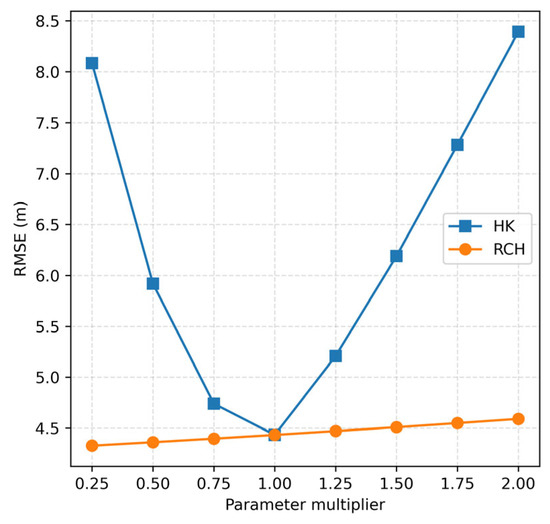
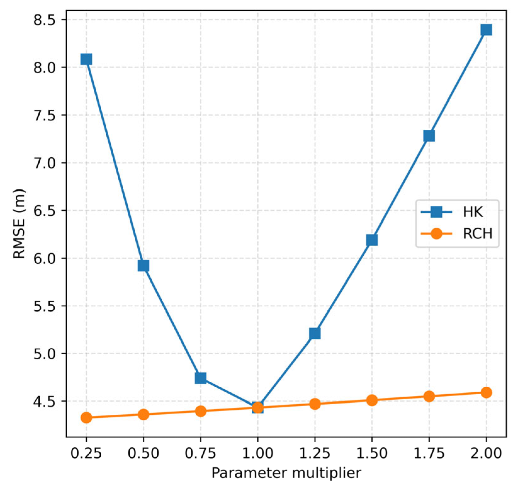
To assess parameter uncertainty, a sensitivity analysis was performed for recharge rate and HK values (Figure 5). Each parameter was varied using multipliers of 0.25, 0.50, 0.75, 1.00, 1.25, 1.50, 1.75, and 2.00, where 1.00 represents the calibrated baseline model. The sensitivity analysis showed that HK was more sensitive than the recharge rate. The RMSE response to HK showed a clear U-shaped pattern, with the lowest error occurring near the calibrated baseline value. The recharge rate exhibited a relatively small influence on RMSE response under the steady-state calibration conditions, suggesting that recharge uncertainty has a smaller influence on calibration error.
Figure 5.
Sensitivity of simulated groundwater head to horizontal hydraulic conductivity (HK) and recharge (RCH). The model response was evaluated using RMSE between the observed and simulated groundwater head.
The findings highlight the importance of the borehole-derived geological model and HK zoning. On the other hand, the geological system is constrained by a limited number of boreholes, and uncertainty in HK value is an important limitation of the study, which should be reduced in future work using additional boreholes, hydraulic tests, and field experiments.
3.2. Model Calibration
Figure 6b,c show the hydraulic conductivities of the shallow and deep aquifers after calibration. The calibrated results reveal a heterogeneous distribution of hydraulic conductivities across the basin. The distribution is consistent with the geological complexity of the basin, where an alluvial fan is filled with deposited sediment and surrounded by mountain-derived materials at the edge of the basin.
Figure 6.
Hydraulic conductivity zonation for parameter estimation (PEST) calibration and calibrated hydraulic conductivity distribution for the Kofu Basin groundwater model. (a) Hydraulic conductivity zones (blue polygons; zones 1–9) and the pilot points (red dots) used for PEST calibration. (b) Calibrated hydraulic conductivity distribution for the shallow aquifer. (c) Calibrated hydraulic conductivity distribution for the deep aquifer.
The calibrated shallow aquifer conductivity in Figure 6b shows relatively high conductivity over the lowland area, consistent with the Kamanashi and Fuefuki River alluvial fans, where coarse and sandy material dominate and groundwater flow is rapid. This condition facilitates groundwater recharge in the shallow aquifer through surface runoff infiltration and mountain-derived recharge. Conversely, lower conductivity zones occur locally around the basin margins. Therefore, the shallow aquifer is characterized by strong local-scale variability.
Composed primarily of compact sand, tuff, and fractured volcanic rocks, the deep aquifer (Figure 6c) exhibits lower hydraulic conductivities and a more regionally coherent conductivity pattern than the shallow aquifer. High conductivity remains prominent in the southern basin and parts of the central area, whereas lower conductivity is distributed toward the western and eastern margins due to granite. This pattern indicates that the deeper groundwater system is less controlled by local-scale surface depositional variability and more controlled by the broader basin structure. In general, shallow aquifers reflect more localized heterogeneity, whereas deep aquifers reflect the larger-scale stratigraphic structure of the basin.
The contrast and distribution of the calibrated hydraulic conductivity values appear to be hydrogeologically plausible and provide an important basis for interpreting the simulated groundwater flow system. These values reflect the potential to transfer water from precipitation to the shallow aquifer, indicating local precipitation recharge, short flow paths, and partial MFR rather than a fully integrated regional flow system. Therefore, the mountain recharge signal in the shallow aquifer may be spatially diffuse and less clearly expressed. In contrast, the deep aquifer exhibits a smoother and more regionally coherent conductivity pattern, which is favorable for regional groundwater flow paths and mountain groundwater transmission over long distances. This suggests that mountain recharge is more effectively incorporated into the deeper groundwater system than into the shallow system.
3.3. Simulated Groundwater Head
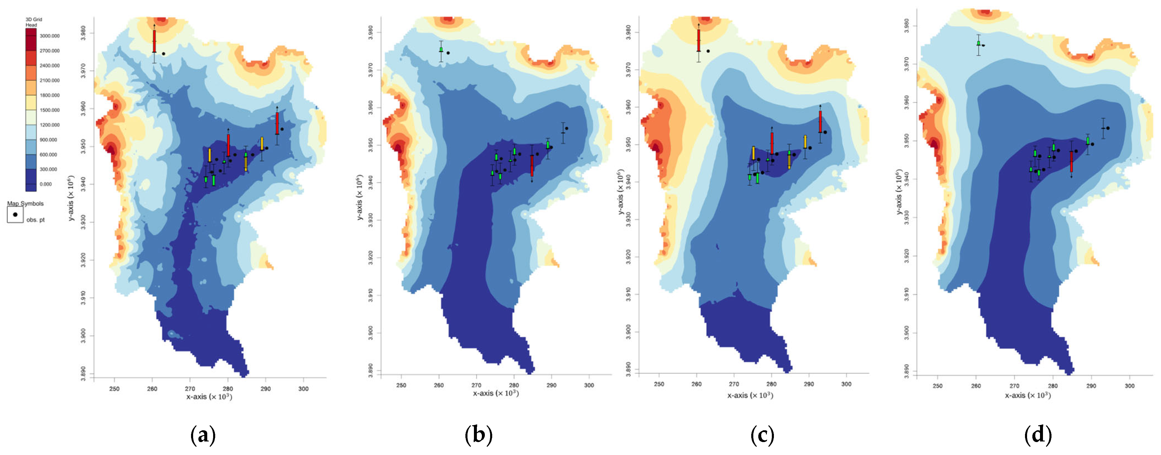
The simulated groundwater head distribution is shown in Figure 7, providing important insights into the groundwater flow dynamics of the Kofu Basin and how calibration and climate data improved the groundwater model. The water budgets of both the initial models and the calibrated model are shown in Table A1 and Table A2, which were used to quantify the groundwater inflow and outflow components.
Figure 7.
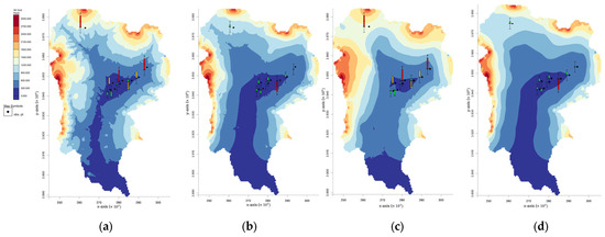
Simulated groundwater head distribution of shallow and deep aquifers before and after model calibration using QSWAT+ recharge. (a–d) show the simulated heads for the shallow and deep aquifers, respectively. Black dots denote observation wells. Colored vertical bars show the observed groundwater head and associated uncertainty interval (±3 m standard deviation) used in model calibration.
In the initial model (Figure 7a,c), the shallow and deep aquifers exhibited inaccurate flow patterns and notable differences from the observed heads, particularly in the region near the mountain foothills. The differences resulted from uniform recharge and hydraulic conductivity, which did not reflect the strong spatial heterogeneity of the river catchment. The shallow and deep aquifers of the initial model illustrated excessive head, especially in the adjacent mountain area. This phenomenon suggests that the limitation of subsurface outflow results in groundwater buildup beneath mountain blocks but cannot be distributed to lowland areas.
In contrast, the simulated model based on QSWAT+ climate data exhibited considerable improvement, yielding a spatial pattern consistent with the field observations (Figure 7b,d). The shallow groundwater head is highly consistent with the interpolated head from domestic groundwater wells, confirming the accuracy of the simulation. In the deep aquifer, the head gradient is smoother and more stable, along with the results of Nguyen et al. [26] in deep groundwater, suggesting that the deep groundwater is more influenced by regional flow. The calibrated simulation reproduced more realistic groundwater flow patterns, demonstrating that the calibrated model based on QSWAT+ data better captured the infiltration processes and groundwater flow dynamics occurring along the fan.
3.4. Model Performance
The performance of the initial and calibrated models was evaluated and presented in two scatter plots (Figure 8). The dashed line represents the 1:1 line, and the solid blue line represents the regression fit between the simulated and observed heads. The initial model showed a high coefficient of determination (R2) of 0.99. However, the relatively large root mean square error (RMSE) of 50.8631 m, mean absolute error (MAE) of 21.0932 m, and Nash–Sutcliffe efficiency (NSE) of 0.9530 indicate substantial errors in the simulated head. The normalized root mean square error (NRMSE) was calculated to evaluate the magnitude of RMSE relative to the observed groundwater level range. The initial model produced NRMSE = 5.91%, showing large normalized errors, although these remained still small relative to the basin-scale groundwater head variation. The regression slope of 1.2 and the intercept of −52.08 indicate a marked bias, with the model tending to overestimate groundwater head. Therefore, the initial model was unable to fully reproduce the observed groundwater system.
Figure 8.
Comparison of observed and simulated groundwater head for initial (a) and calibrated (b) models using climate data from the QSWAT+ simulation.
After applying PEST calibration and climate data input from QSWAT+, the model performance markedly improved. The regression equation, y = 1.00x + 0.12, indicates that the fitted relationship nearly matches the observed data. The RMSE decreased from 50.8631 to 4.4331 m, representing a 91.28% reduction in the total error, with an NRMSE of 0.52%, whereas the MAE improved by 84.38% (from 21.0932 to 3.2955 m). The NSE increased from 0.9530 to 0.9996, indicating substantially improved model performance and the correspondence between the observed and simulated groundwater head. The results demonstrate that integrating hydrological input data from QSWAT+ with the MODFLOW model can enhance the reliability of the groundwater flow simulation.
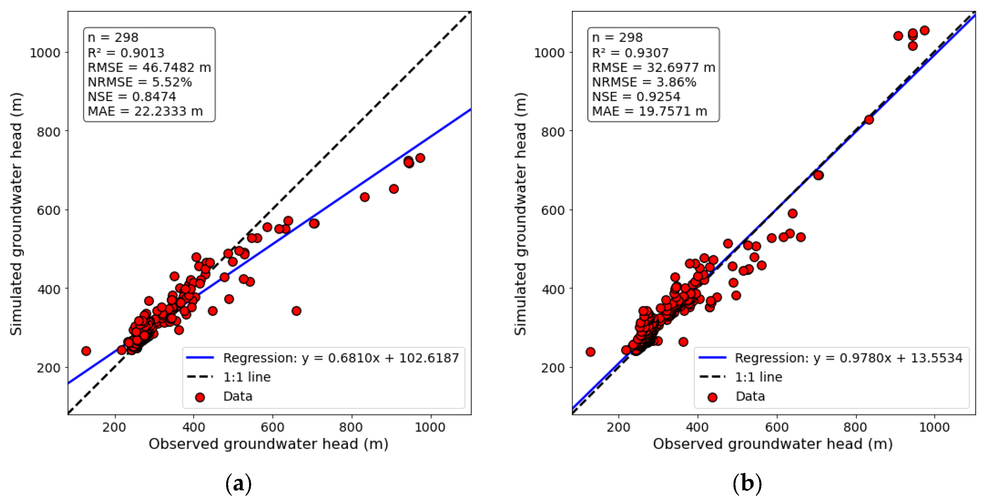
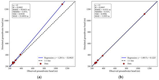
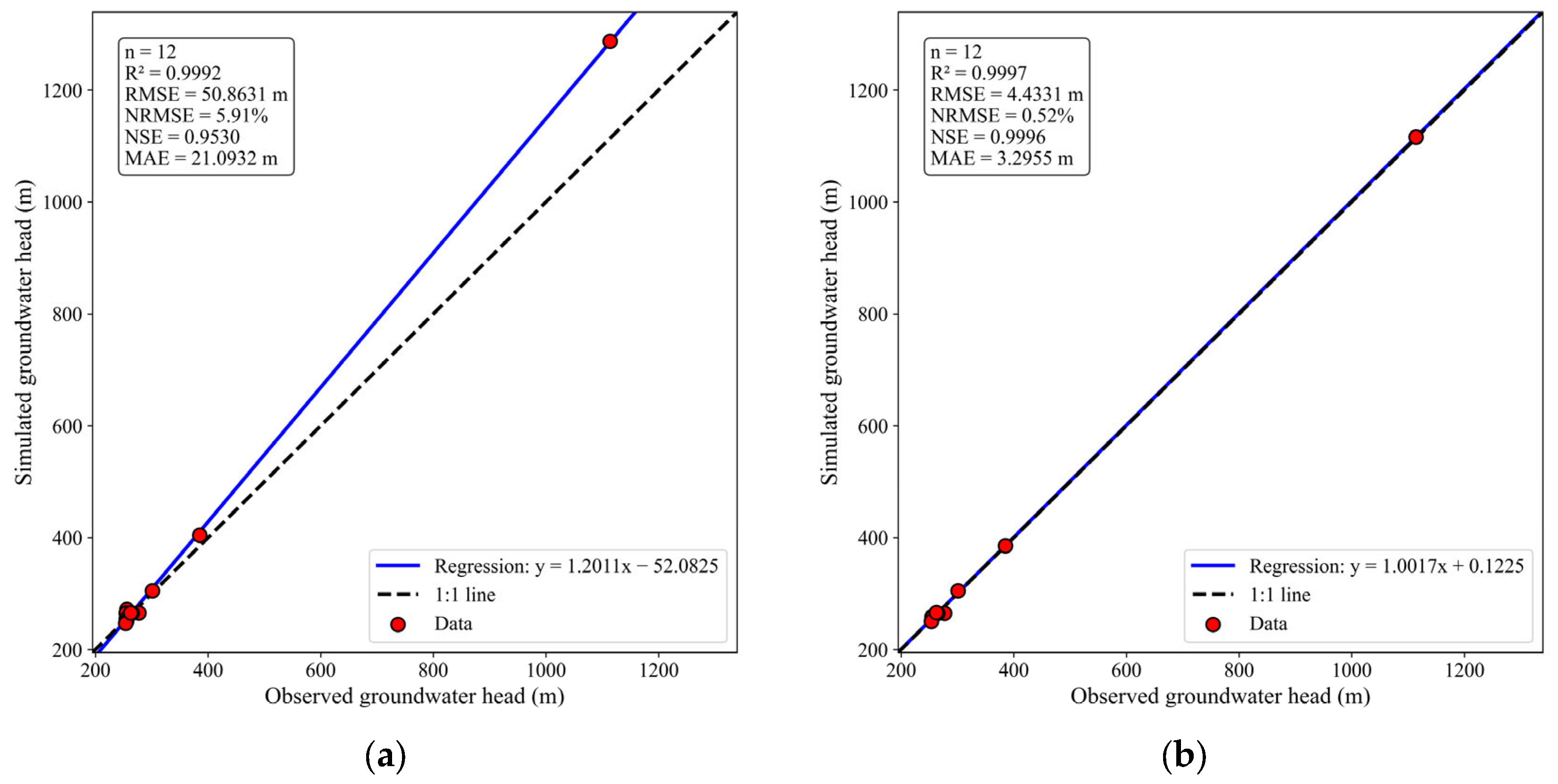
The calibrated model was further evaluated using an independent dataset of 298 domestic and geological wells with measured groundwater levels (Figure A1). Compared with the initial model, the MODFLOW simulation using QSWAT+-derived data shows stronger agreement between observed and simulated groundwater head. The R2 and NSE values were 0.9307 and 0.9254, respectively, indicating that the model reasonably captured the general groundwater head trend across the study area. However, RMSE and MAE remained relatively high at 32.70 m and 19.76 m, respectively, particularly for wells located at higher elevations. This indicates that local-scale discrepancies persist. These errors are likely related to limited geological borehole and observation-well data in remote and high-elevation areas. In addition, the absence of detailed pumping and irrigation data increases uncertainty in the simulation.
Compared with recent studies on the groundwater flow model using SWAT–MODFLOW [34], MODFLOW model using uniform recharge [35], and semi-uniform recharge [36] (Table A3), the model performance was stronger at the calibrated model. The validation showed better results in capturing the basin-scale groundwater level. Despite remaining relatively large errors in value, NRMSE is still accepted for basin-scale model performance. The statistics have confirmed that the model should be interpreted as a basin-scale representation of regional groundwater flow patterns. The local groundwater head predictive accuracy across the basin needs more attention on the availability of climate and hydrogeological data.
From a hydrogeological perspective, this improvement suggests that recharge distribution has a notable influence on groundwater levels in the Kofu Basin. The initial model relied on uniform recharge assumptions and could not represent the spatial recharge distribution in the mountainous area. In contrast, the calibrated simulation incorporated climate-driven recharge patterns, which better reflect differences in topography, land surface conditions, and hydrological inputs. Consequently, the model could represent the groundwater system more realistically, thereby remarkably improving the simulation accuracy.
3.5. Velocity Vector and Comparison with Groundwater Recharge Sources from Stable Isotope Studies
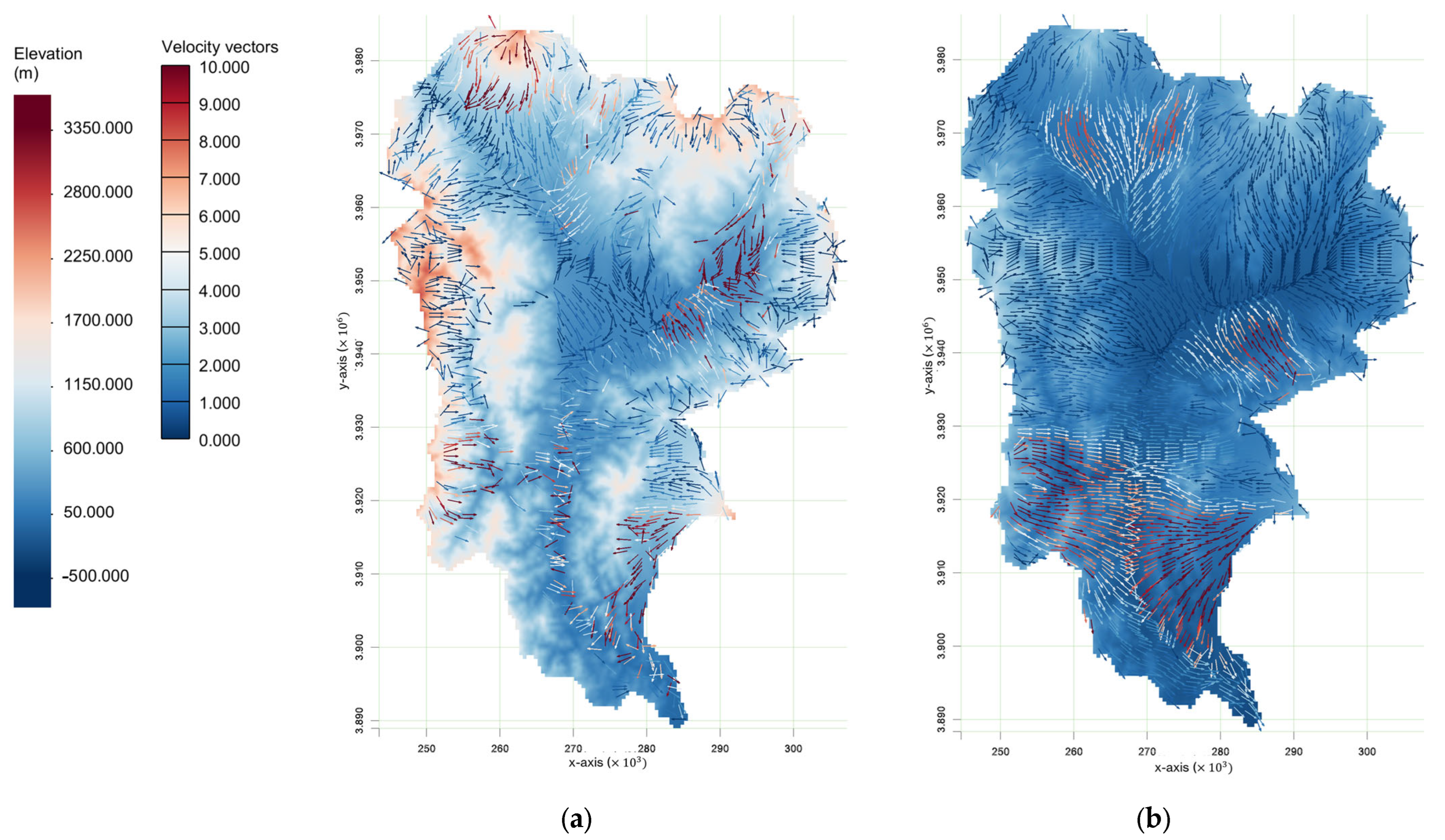
Figure 9 shows the simulated groundwater flow directions and magnitudes represented by velocity vectors and elevation contours. In the shallow aquifer (Figure 9a), the vectors are relatively scattered and spatially heterogeneous, with stronger velocities concentrated primarily along the main rivers and near the mountain edge. The groundwater flows downslope and toward the basin center, indicating a rapid subsurface flow through highly permeable sand and gravel deposits. This demonstrates a strong connection between surface recharge and the unconfined groundwater system in the mountain areas of the north and east. This behavior is typical of a shallow groundwater system that responds rapidly to local precipitation, river interaction, and MFR in the upper basin-fill deposits.
Figure 9.
Groundwater velocity vectors in the Kofu Basin overlaid on elevation for shallow (a) and deep (b) aquifers. Arrow orientation shows the direction of groundwater movement, and arrow color corresponds to flow velocity magnitude.
In contrast, the deep aquifer (Figure 9b) exhibits a coherent and regionally integrated flow pattern. The velocity vectors are smoother and are continuously directed from the surrounding mountain areas toward the basin interior. The pattern is consistent with the possible contribution of mountain-derived recharge. The convergence of the vectors at the basin center suggests regional groundwater transmission. Therefore, the deep aquifer preserves the regional recharge signal more clearly than the shallow aquifer.
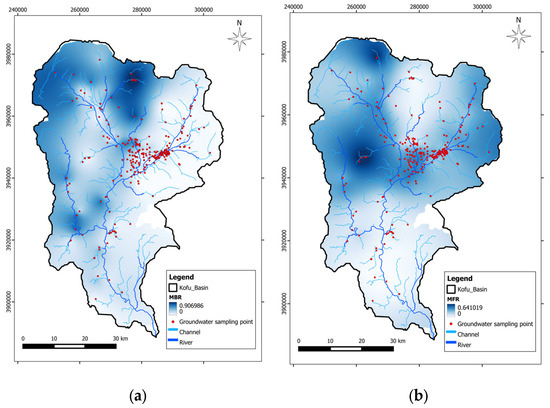
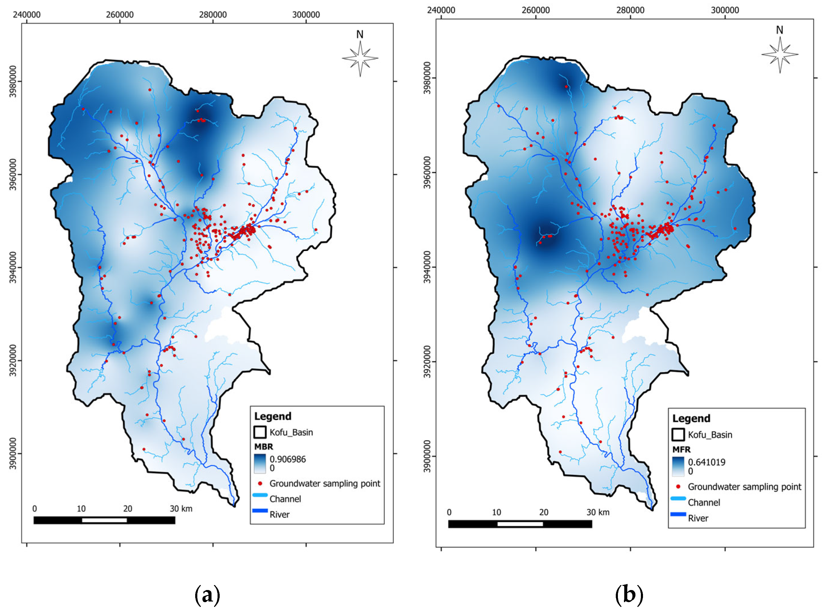
The contrast and distribution between shallow and deep flow fields are particularly important when interpreted together with the mountain recharge results of the Kofu Basin discussed in a previous study by Nguyen et al. (2025) [26]. The previous analysis identified distinct groundwater recharge contributions associated with the Yatsugatake, Chichibu, and Minimi Alps mountain areas (Figure 10). In particular, areas of higher MBR contribution are distributed mainly toward the western and northwestern parts of the basin (Figure 10a). The simulated deep groundwater flow vectors are broadly consistent with this spatial pattern because they indicate regional basinward flow from the surrounding mountain margins toward the basin interior.
Figure 10.
Spatial distribution of the main recharge source in the Kofu Basin after the mountain recharge study by Nguyen et al. (2025) [26]. (a) mountain-block recharge (MBR), and (b) mountain-front recharge (MFR). The red dots indicate groundwater sampling points.
MFR is more likely associated with the transition zone between mountains and basin alluvial fans, where runoff and subsurface flow emerging from the uplands infiltrate into coarse alluvial fan and piedmont deposits (Figure 10b). This behavior corresponds well to the simulated velocities from the groundwater flow model and reflects the concentration of recharge along the mountain–plain transition. In addition, the MBR and MFR ratio was used as soft information during the SWAT+ calibration stage to guide the representation of spatial recharge processes. Therefore, these values were not treated as independent quantitative recharge source estimates in the MODFLOW analysis.
These results suggest that mountain recharge and groundwater dynamics in the Kofu Basin are spatially heterogeneous and depth-dependent. The deeper aquifer served as the primary regional flow domain through which mountain groundwater was transmitted. The velocity structure emphasizes the characteristics of recharge processes in the basin. This interpretation strengthens the concept of mountain groundwater recharge by multiple groundwater sources in the mountainous river catchment. These flow directions and magnitudes improve understanding of the groundwater flow regime and support decision-making.
The stable isotope evidence provides an additional line of interpretation beyond the hydraulic head simulation. Flow vectors and head gradients can indicate possible groundwater flow directions, but they cannot by themselves prove recharge origin. By combining simulated regional flow patterns with isotope-based recharge source interpretation, the study provides a more constrained basis for identifying potential mountain-derived recharge contributions.
4. Conclusions
The results of the proposed framework suggest that the geological system in the Kofu Basin is spatially heterogeneous, implying that the groundwater model cannot be adequately represented using spatially uniform recharge and climate-related inputs. The incorporation of recharge and ET rates derived from QSWAT+ outputs improved the simulation of groundwater head and dynamics, supporting the applicability of the coupled modeling approach for representing basin-scale groundwater processes.
The calibrated results of the groundwater flow model reveal a distinction between the shallow and deep aquifers. The shallow aquifer exhibits localized and heterogeneous flow, reflecting the strong influence of local precipitation recharge and near-surface lithological variability. In contrast, the deep aquifer exhibits a regional flow pattern, which is directed from surrounding mountainous areas toward the alluvial fans of the basin, indicating that mountain recharge is clearly expressed in the deep groundwater system.
Analysis of the simulated groundwater flow directions and velocity vectors provides key insights into the dynamic recharge processes of the basin, suggesting that the surrounding uplands act as important recharge source areas, particularly along the northern, eastern, and southwestern margins of the basin. These results are consistent with the recharge distribution inferred from the end-member mixing analysis results, which identified contributions from local precipitation, MBR, and MFR. Thus, the numerical model provides a groundwater dynamics explanation for the source apportionment identified by the geochemical analysis.
This result supports the findings that mountain water plays a major role in sustaining groundwater in the Kofu Basin. The consistency among groundwater head calibration, modeled flow directions, recharge zoning, and independent hydrochemical evidence strengthens confidence in the conceptual model and reduces uncertainty in recharge area identification. However, independent validation showed remaining local-scale errors; the model should be interpreted as a basin-scale tool for evaluating regional groundwater flow and recharge processes, rather than as a precise predictor of groundwater head at individual wells.
Overall, this study demonstrates the potential of integrating QSWAT+ climate outputs, groundwater flow modeling, and independent geochemical evidence to provide a practical framework for identifying recharge processes in the Kofu Basin. The output could be used as a basin-scale hydrological interpretation, providing critical insights into the groundwater system, which can support future groundwater management scenario analysis, planning, and policy-making. Model uncertainty remains due to limited observation wells coverage, hydrostratigraphic heterogeneity, and the lack of sufficient field-based hydraulic measurements.
Author Contributions
Conceptualization, C.Q.N. and T.N.; methodology, C.Q.N. and T.N.; software, C.Q.N.; validation, C.Q.N.; formal analysis, C.Q.N.; resources, C.Q.N. and T.N.; data curation, C.Q.N. and T.N.; writing—original draft preparation, C.Q.N.; writing—review and editing, C.Q.N. and T.N.; visualization, C.Q.N.; supervision, T.N.; funding acquisition, T.N. All authors have read and agreed to the published version of the manuscript.
Funding
This research received no external funding.
Data Availability Statement
The data that support the findings of this study—including stable isotope ratios, climate, and geological borehole data—are available from the corresponding author upon reasonable request.
Acknowledgments
The author would like to extend special gratitude to the Interdisciplinary Center for River Basin Environment (ICRE) and the research team for their valuable support, guidance, and resources.
Conflicts of Interest
The authors declare no conflicts of interest.
Abbreviations
The following abbreviations are used in this manuscript:
| CHD | Constant head package |
| ET | Evapotranspiration |
| EVT | Evapotranspiration package |
| GMS | Groundwater Modeling System |
| MAE | Mean absolute error |
| MBR | Mountain block recharge |
| MFR | Mountain front recharge |
| MODFLOW | Modular finite-difference groundwater flow model |
| MODFLOW-NWT | MODFLOW with Newton formulation/Newton solver |
| NSE | Nash–Sutcliffe efficiency |
| PEST | Parameter Estimation algorithm |
| RCH | Recharge package/Recharge |
| RIV | River package |
| RMSE | Root mean square error |
| STR | Stream package |
| UPW | Upstream Weighting package |
Appendix A
Table A1.
The quantitative flux balance of the initial model.
Table A2.
The quantitative flux balance of the calibrated model.
Table A3.
Comparison of groundwater head simulation performance with recent groundwater flow model studies.
Figure A1.
Independent validation of simulated groundwater head using 298 domestic wells: (a) initial model and (b) models using climate data from the QSWAT+ simulation. The dashed line represents the 1:1 line, and the blue line represents the linear regression between observed and simulated groundwater head.
References
- Markovich, K.H.; Manning, A.H.; Condon, L.E.; McIntosh, J.C. Mountain-block recharge: A review of current understanding. Water Resour. Res. 2019, 55, 8278–8304. [Google Scholar] [CrossRef] [Scilit]
- Viviroli, D.; Weingartner, R. The hydrological significance of mountains: From regional to global scale. Hydrol. Earth Syst. Sci. 2004, 8, 1017–1030. [Google Scholar] [CrossRef] [Scilit]
- Zektser, I.; Loaiciga, H.A. Groundwater fluxes in the global hydrologic cycle: Past, present and future. J. Hydrol. 1993, 144, 405–427. [Google Scholar] [CrossRef] [Scilit]
- Pinder, G.F. Groundwater Hydrology. Groundwater Quantity and Quality Management, 3rd ed.; John Wiley and Sons, Inc.: Hoboken, NJ, USA, 2011; pp. 10–35. [Google Scholar]
- Kuang, X.; Liu, J.; Scanlon, B.R.; Jiao, J.J.; Jasechko, S.; Lancia, M.; Biskaborn, B.K.; Wada, Y.; Li, H.; Zeng, Z. The changing nature of groundwater in the global water cycle. Science 2024, 383, eadf0630. [Google Scholar] [CrossRef] [Scilit] [PubMed]
- Shaikh, M.; Birajdar, F. Groundwater and ecosystems: Understanding the critical interplay for sustainability and conservation. EPRA Int. J. Multidiscip. Res. 2024, 10, 181–186. [Google Scholar] [CrossRef] [Scilit]
- Jwan, S.M.; Mawlood, D.K. Developing three-dimensional groundwater flow modeling for the Erbil Basin using Groundwater Modeling System (GMS). J. Groundw. Sci. Eng. 2024, 12, 178. [Google Scholar] [CrossRef] [Scilit]
- Pande, C.B.; Moharir, K.N.; Singh, S.K.; Elbeltagi, A.; Pham, Q.B.; Panneerselvam, B.; Varade, A.M.; Kouadri, S. Groundwater flow modeling in the basaltic hard rock area of Maharashtra, India. Appl. Water Sci. 2022, 12, 12. [Google Scholar]
- Cho, J.; Mostaghimi, S.; Kang, M. Development and application of a modeling approach for surface water and groundwater interaction. Agric. Water Manag. 2010, 97, 123–130. [Google Scholar] [CrossRef] [Scilit]
- Yuan, L.R.; Xin, P.; Kong, J.; Li, L.; Lockington, D. A coupled model for simulating surface water and groundwater interactions in coastal wetlands. Hydrol. Process. 2011, 25, 3533–3546. [Google Scholar] [CrossRef] [Scilit]
- Xu, S.; Frey, S.; Erler, A.; Khader, O.; Berg, S.; Hwang, H.; Callaghan, M.; Davison, J.; Sudicky, E. Investigating groundwater-lake interactions in the Laurentian Great Lakes with a fully-integrated surface water-groundwater model. J. Hydrol. 2021, 594, 125911. [Google Scholar] [CrossRef] [Scilit]
- Davamani, V.; John, J.E.; Poornachandhra, C.; Gopalakrishnan, B.; Arulmani, S.; Parameswari, E.; Santhosh, A.; Srinivasulu, A.; Lal, A.; Naidu, R. A Critical Review of Climate Change Impacts on Groundwater Resources: A Focus on the Current Status, Future Possibilities, and Role of Simulation Models. Atmosphere 2024, 15, 122. [Google Scholar] [CrossRef] [Scilit]
- Ojha, R.; Ramadas, M.; Govindaraju, R.S. Current and future challenges in groundwater. I: Modeling and management of resources. J. Hydrol. Eng. 2015, 20, A4014007. [Google Scholar] [CrossRef] [Scilit]
- Refsgaard, J.C.; Højberg, A.L.; Møller, I.; Hansen, M.; Søndergaard, V. Groundwater modeling in integrated water resources management—Visions for 2020. Groundwater 2010, 48, 633–648. [Google Scholar] [CrossRef] [Scilit]
- Wang, S.-J.; Nguyen, Q.C.; Lu, Y.-C.; Doyoro, Y.G.; Tran, D.-H. Evaluation of geological model uncertainty caused by data sufficiency using groundwater flow and land subsidence modeling as example. Bull. Eng. Geol. Environ. 2022, 81, 331. [Google Scholar] [CrossRef] [Scilit]
- Mohan, C.; Western, A.W.; Wei, Y.; Saft, M. Predicting groundwater recharge for varying land cover and climate conditions–a global meta-study. Hydrol. Earth Syst. Sci. 2018, 22, 2689–2703. [Google Scholar] [CrossRef] [Scilit]
- Moeck, C.; Brunner, P.; Hunkeler, D. The influence of model structure on groundwater recharge rates in climate-change impact studies. Hydrogeol. J. 2016, 24, 1171–1184. [Google Scholar] [CrossRef] [Scilit]
- Kumar, C. Groundwater Flow Models; Scientist ‘E1’ National Institute of Hydrology Roorkee–247667 (Uttaranchal) Publication: Roorkee, India, 2002. [Google Scholar]
- Panagopoulos, G. Application of MODFLOW for simulating groundwater flow in the Trifilia karst aquifer, Greece. Environ. Earth Sci. 2012, 67, 1877–1889. [Google Scholar] [CrossRef] [Scilit]
- Niswonger, R.G.; Panday, S.; Ibaraki, M. MODFLOW-NWT, a Newton formulation for MODFLOW-2005. US Geol. Surv. Tech. Methods 2011, 6, 44. [Google Scholar]
- Borzì, I. Modeling Groundwater Resources in Data-Scarce Regions for Sustainable Management: Methodologies and Limits. Hydrology 2025, 12, 11. [Google Scholar] [CrossRef] [Scilit]
- Van Camp, M.; Mjemah, I.C.; Al Farrah, N.; Walraevens, K. Modeling approaches and strategies for data-scarce aquifers: Example of the Dar es Salaam aquifer in Tanzania. Hydrogeol. J. 2013, 21, 341–356. [Google Scholar]
- Bailey, R.T.; Bieger, K.; Flores, L.; Tomer, M. Evaluating the contribution of subsurface drainage to watershed water yield using SWAT+ with groundwater modeling. Sci. Total Environ. 2022, 802, 149962. [Google Scholar] [CrossRef] [Scilit] [PubMed]
- Bailey, R.T.; Park, S.; Bieger, K.; Arnold, J.G.; Allen, P.M. Enhancing SWAT+ simulation of groundwater flow and groundwater-surface water interactions using MODFLOW routines. Environ. Model. Softw. 2020, 126, 104660. [Google Scholar] [CrossRef] [Scilit]
- Izady, A.; Davary, K.; Alizadeh, A.; Ziaei, A.; Akhavan, S.; Alipoor, A.; Joodavi, A.; Brusseau, M. Groundwater conceptualization and modeling using distributed SWAT-based recharge for the semi-arid agricultural Neishaboor plain, Iran. Hydrogeol. J. 2015, 23, 47–68. [Google Scholar]
- Nguyen, Q.C.; Kimura, T.; Nakamura, T. Evaluating mountain recharge in Yamanashi, Japan, using stable isotopes and a hydrogeological groundwater flow model. Hydrol. Res. 2025, 56, 951–966. [Google Scholar] [CrossRef] [Scilit]
- Sawaki, Y.; Asanuma, H.; Abe, M.; Hirata, T. U–Pb ages of granitoids around the Kofu basin: Implications for the Neogene geotectonic evolution of the South Fossa Magna region, central Japan. Isl. Arc 2020, 29, e12361. [Google Scholar] [CrossRef] [Scilit]
- Matsuda, T. Collision of the Izu-Bonin arc with central Honshu: Cenozoic tectonics of the Fossa Magna, Japan. J. Phys. Earth 1978, 26, S409–S420. [Google Scholar] [CrossRef] [Scilit]
- McDonald, M.G.; Harbaugh, A.W. A Modular Three-Dimensional Finite-Difference Ground-Water Flow Model; US Geological Survey: Reston, VA, USA, 1988. [Google Scholar]
- Khan, S.; Rana, T.; Gabriel, H.; Ullah, M.K. Hydrogeologic assessment of escalating groundwater exploitation in the Indus Basin, Pakistan. Hydrogeol. J. 2008, 16, 1635–1654. [Google Scholar] [CrossRef] [Scilit]
- Earle, S. Physical Geology; BC Campus: Chestnut Hill, MA, USA, 2015. [Google Scholar]
- Kim, N.W.; Chung, I.M.; Won, Y.S.; Arnold, J.G. Development and application of the integrated SWAT–MODFLOW model. J. Hydrol. 2008, 356, 1–16. [Google Scholar] [CrossRef] [Scilit]
- Aslam, R.A.; Shrestha, S.; Usman, M.N.; Khan, S.N.; Ali, S.; Sharif, M.S.; Sarwar, M.W.; Saddique, N.; Sarwar, A.; Ali, M.U. Integrated SWAT-MODFLOW modeling-based groundwater adaptation policy guidelines for Lahore, Pakistan under projected climate change, and human development scenarios. Atmosphere 2022, 13, 2001. [Google Scholar] [CrossRef] [Scilit]
- Sisay, B.M.; Nedaw, D.; Birhanu, B.; Gigar, A.G. Application of SWAT and MODFLOW models for characterization of surface–groundwater interaction in the Modjo River catchment, central Ethiopia. Environ. Earth Sci. 2023, 82, 341. [Google Scholar] [CrossRef] [Scilit]
- Belay, A.S.; Yenehun, A.; Nigate, F.; Nigussie, W.; Tilahun, S.A.; Dessie, M.; Moges, M.M.; Chen, M.; Adgo, E.; Fentie, D. Investigation of interbasin groundwater flow using multiple approaches: The case of the Tana and Beles basins, Ethiopia. Hydrogeol. J. 2023, 31, 2251–2270. [Google Scholar] [CrossRef] [Scilit]
- Raazia, S.; Dar, A.Q. A numerical model of groundwater flow in Karewa-Alluvium aquifers of NW Indian Himalayan Region. Model. Earth Syst. Environ. 2022, 8, 871–882. [Google Scholar]
- Gebru, H.; Gebreyohannes, T.; Hagos, E.; Perilli, N. Hydrogeological Assessment and Steady-State Groundwater Flow Modeling for Groundwater Management in the Golina River Sub-Basin, Northern Ethiopia, Using MODFLOW 6. Water 2025, 17, 949. [Google Scholar] [CrossRef] [Scilit]

Disclaimer/Publisher’s Note: The statements, opinions and data contained in all publications are solely those of the individual author(s) and contributor(s) and not of MDPI and/or the editor(s). MDPI and/or the editor(s) disclaim responsibility for any injury to people or property resulting from any ideas, methods, instructions or products referred to in the content. |
© 2026 by the authors. Licensee MDPI, Basel, Switzerland. This article is an open access article distributed under the terms and conditions of the Creative Commons Attribution (CC BY) license.