Decoupling Geometric and Area Effects on Denil Fishway Hydrodynamics at Equivalent Openness Ratios

Abstract

Denil fishways exhibit limited passage efficiency for weak-swimming and benthic species, partly due to severe near-bed hydrodynamics generated by the sharp V-notch apex of conventional baffles. Modifying bottom geometry is a promising optimization pathway, but previous studies often lack rigorous comparison under constrained baffle openness ratios. This study employed CFD with the RNG $k-\epsilon$ turbulence model to evaluate conventional V-shaped (TDF), equivalent U-shaped (SCDF), and rectangular (RDF) baffles under a unified openness ratio. A layered hydrodynamic evaluation framework demarcated by the effective blocking height was developed to distinguish flow responses in the upper jet-dominated and lower baffle-controlled layers. Results show that the upper-layer conveyance indicators remain broadly comparable across configurations, whereas the lower-layer indicators show configuration-related differences within the tested discharge range. The RDF and SCDF reduce lower-layer mean velocity and TKE relative to the TDF baseline across the tested discharge range, with the RDF achieving the larger velocity reduction and the SCDF the larger TKE reduction. The maximum relative reduction in lower-layer TKE, approximately 22%, occurs under intermediate discharge. These results suggest that bottom baffle geometry can provide a potential means of adjusting near-bed hydraulic conditions in Denil fishways, although the ecological consequences require further verification.

1. Introduction

Longitudinal connectivity of river networks is a fundamental ecological prerequisite for maintaining the population integrity of migratory fish and freshwater biodiversity [1,2]. However, the global proliferation of dams and sluices has fragmented more than two-thirds of major river systems [3,4], causing unprecedented habitat degradation for migratory species [5,6,7]. While fishways have been deployed for over three centuries as the primary engineering mitigation strategy [8,9], extensive field evaluations reveal that average upstream passage efficiency remains alarmingly low at approximately 41.7%. This persistent shortfall is largely attributed to conventional designs being tailored to strong-swimming salmonids, generating hydraulic conditions (e.g., high velocities and steep gradients) that exceed the capacities of many weak-swimming and benthic species [10]. To overcome this efficiency bottleneck, fishway design must shift from broad matching of macroscopic hydrological parameters toward refined optimization of near-field hydrodynamic conditions [11].

While various technical fishways have been developed, their selection depends on the swimming capabilities of target species, local hydrological regimes, and site-specific spatial constraints [10,12]. Vertical-slot fishways (VSFs), for instance, are widely favored for their adaptability to full-depth flow passage and large water level fluctuations [13,14]. Nevertheless, their substantial spatial footprint renders them economically or physically impractical in high-head or space-constrained projects. In such cases, the Denil fishway, characterized by its compact structure and adaptability to steep gradients [15,16], represents a practical alternative. This configuration has been extensively implemented and validated for anadromous species, particularly salmonids, across high-gradient river reaches [16,17,18].

The internal geometry of a Denil fishway, featuring a series of 45° inclined baffles, inherently induces a characteristic vertical dual-flow regime [19]. The upper jet-dominated layer features high-velocity longitudinal flow serving as the primary swimming corridor for upstream migration, whereas the lower baffle-controlled layer forms a large-scale recirculation zone essential for fish recovery. Nevertheless, the sharp V-notch apex of conventional baffles generates intense local turbulence, driving high-velocity flow toward the channel bed and compressing the low-velocity, low-turbulence resting space near the bed [19,20]. Such reduction in near-bed refuge space is widely recognized as a primary hydrodynamic barrier limiting passage efficiency for weak-swimming and benthic species, including small-bodied cyprinids and bottom-dwelling fish such as loaches and gobies [21,22]. Consequently, modifying the bottom cross-sectional geometry of baffles to suppress this shear generation at its origin is considered a highly promising approach to optimize near-bed microhabitats for these target species groups.

Recent engineering efforts have attempted to optimize internal flow fields by modifying baffle bottom topologies (e.g., triangular, semicircular, and rectangular) [23]. However, previous studies typically optimized baffle shapes while only keeping the bottom elevation constant, without matching the openness ratio. This likely stems from an implicit assumption that holding bottom elevation constant is sufficient to ensure comparable openings across configurations; while approximately valid for the triangular V-notch, this assumption does not hold for shaped baffles, whose flow-through area varies with the bottom geometry even at an identical bottom elevation. As a result, the openness ratio has rarely been treated as a variable that must be held constant, even though geometric alterations under an uncontrolled openness ratio inevitably cause systematic shifts in bulk discharge distribution and backwater profiles. The shape effect thus becomes inseparable from the area effect, making it impossible to isolate how local geometric features alone regulate flow topology. A second limitation concerns evaluation methodology: conventional studies quantify low-velocity or turbulence zones using cross-sectional averages [24,25]. In Denil fishways, high-magnitude data from the upper main jet systematically dominate bulk averages, masking localized hydrodynamic improvements in the lower resting zone. Consequently, such bulk metrics mask the localized hydrodynamic improvements in the lower resting zone, rendering them hydraulically invisible.

To bridge these critical knowledge gaps, this study employs 3D computational fluid dynamics (CFD) to elucidate the effects of local baffle geometry on the topological structure and energy redistribution within Denil fishways. By enforcing a unified baffle openness ratio to eliminate area-effect interference, three bottom configurations (traditional V-shaped, equivalent U-shaped, and equivalent rectangular) are systematically evaluated. Additionally, a layered hydrodynamic evaluation framework demarcated by the effective blocking height is proposed to distinguish flow responses within the upper jet-dominated and lower baffle-controlled layers. The remainder of this paper is organized as follows. Section 2 describes the geometric equivalence derivation, the numerical modeling framework, and the layered evaluation system. Section 3 presents the flow field analysis across longitudinal and cross-sectional views, the streamwise evolution of hydrodynamic characteristics, and a layered quantitative assessment of baffle configuration effects. Section 4 summarizes the main findings and their practical engineering implications.

2. Methodology

2.1. Baffle Configuration Design

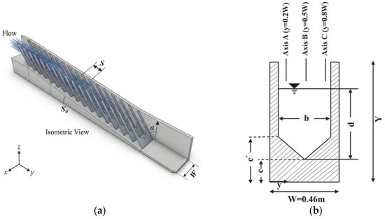
In this study, the standard Denil fishway defined by Odeh [16] was selected as the benchmark geometric model. This dimensioning system not only serves as the normative basis for current fishway engineering designs but also acts as a widely adopted reference configuration for numerous physical experiments and numerical simulations. To eliminate interference from the main channel’s geometric parameters, the longitudinal spacing of the baffles was fixed at $S=0.30 \mathrm{m}$ (equivalent to a relative spacing $S/W=0.65$). Daneshfaraz et al. [26] systematically compared multiple baffle spacings and confirmed that $S=0.30 \mathrm{m}$ maximizes the volume of the near-bed energy dissipation zone while yielding the most favorable overall hydrodynamic performance. Figure 1a illustrates the isometric view of the fishway, reflecting its three-dimensional spatial structure, and Figure 1b presents the cross-sectional dimensions of the V-shaped baffle with measurement axes A ($y=0.2W$), B ($y=0.5W$), and C ($y=0.8W$).

Figure 1. Definition sketch of geometric parameters for the Denil fishway: (a) isometric view, where $S$ is the longitudinal baffle spacing and $S_{\mathrm{o}}$ is the fishway slope; (b) cross-sectional dimensions of V-shaped baffle, where $Y$ is total baffle height, $W$ is fishway channel width, $b$ is baffle notch width, $c$ is vertical elevation of the baffle bottom edge, and $c\prime$ is upper inflection elevation of the baffle. Measurement axes A ($y=0.2W$), B ($y=0.5W$), and C ($y=0.8W$) are indicated.

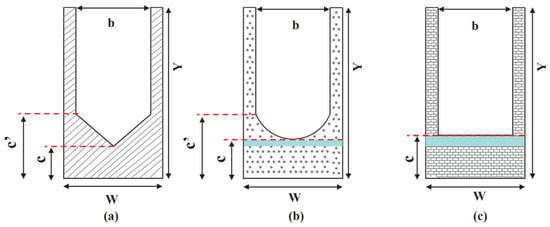
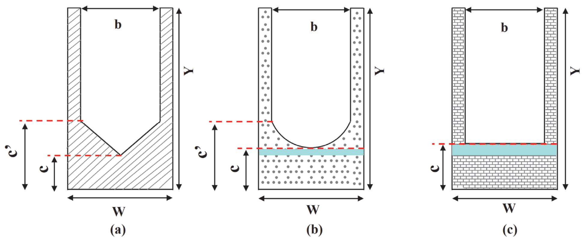
For the parallel comparison of different bottom cross-sectional shapes (V-shaped, U-shaped, and Rectangular), existing studies [23] typically maintain identical notch width b and base elevation c across configurations while varying only in bottom profile geometry. In the present study, these three configurations are referred to as the Traditional Denil Fishway (TDF) for the V-shaped, the Semicircular-bottom Denil Fishway (SCDF) for the U-shaped, and the Rectangular-bottom Denil Fishway (RDF) for the rectangular profile, respectively. As demonstrated in Table 1, geometric alterations inevitably introduce systematic deviations in baffle openness ratio among the three configurations, subsequently biasing their macro-discharge capacities. The openness ratio $P$ is defined as $P=A_{open}/A_{total}$, where $A_{open}$ is the water-crossing area through the baffle opening and $A_{total}$ is the total cross-sectional area of the baffle profile. To isolate the precise regulatory mechanism of baffle geometry on the Denil fishway flow field, this study proposes a geometric equivalence constraint design scheme, as illustrated in Figure 2. Specifically, using the openness ratio of the TDF reference model ($P=54.69\%$) as the fixed constraint target, the bottom elevation parameters of the SCDF and RDF baffles were recalibrated through area integral back-calculations. This approach achieves strict consistency in baffle openness ratio across all three configurations while preserving their respective curvature characteristics and geometric features.

Table 1. Design parameters for the three baffle configurations. (Note: Geometric variables are defined in Figure 1; P denotes the openness ratio, and the Error column represents its relative deviation from the TDF reference model.).

Models	Y (m)	W (m)	b (m)	c (m)	c’ (m)	P	Error
TDF (Reference Model)	0.8	0.46	0.35	0.15	0.3	54.69%	Standard
SCDF (Daneshfaraz et al. [23])	0.8	0.46	0.35	0.15	0.3	58.26%	+3.57%
RDF (Daneshfaraz et al. [23])	0.8	0.46	0.35	0.15	--	61.82%	+7.13%
SCDF (Present study)	0.8	0.46	0.35	0.189	0.3	54.69%	0%
RDF (Present study)	0.8	0.46	0.35	0.225	--	54.69%	0%

Figure 2. Comparison of the three baffle cross-sectional designs: (a) TDF; (b) SCDF; (c) RDF. The blue-shaded regions in (b,c) indicate the geometric modifications relative to Daneshfaraz et al. [23], introduced to enforce a consistent openness ratio.

2.2. Numerical Setup and Model Validation

2.2.1. Governing Equations

Numerical simulations were performed using the STAR-CCM+ platform, employing the three-dimensional incompressible Reynolds-Averaged Navier–Stokes (RANS) equations as the governing framework. Turbulence closure was achieved via the RNG k-ε model. Compared with the standard $k-\epsilon$ formulation, the RNG variant introduces an additional strain-rate term in the $\epsilon$ equation, providing improved accuracy for flows involving rapid deformation and strongly curved shear layers, conditions characteristic of the baffle notch region in Denil fishways. The combined RNG $k-\epsilon$ and VOF framework has been validated against experimental data in vertical-slot and pool-type fishways, demonstrating good performance in free-surface tracking and turbulence prediction [27,28]. The governing equations are expressed as follows:

$${\displaystyle \frac{\partial u_i}{\partial x_i}}=0$$

(1)

$${\displaystyle \frac{\partial {\rho u}_i}{\partial t}}+{\displaystyle \frac{\partial }{\partial x_j}}\left(\rho u_i{u}_j\right)=-{\displaystyle \frac{\partial p}{\partial x_i}}+{\displaystyle \frac{\partial }{\partial x_j}}\left[\mu \left({\displaystyle \frac{\partial u_i}{\partial x_j}}+{\displaystyle \frac{\partial u_j}{\partial x_i}}\right)-\rho \overline{u_i^{\prime }{u}_j^{\prime }}\right]+\rho g_i$$

(2)

where $i=\mathrm{1,2},3$ represents the spatial coordinate components in the Cartesian coordinate system; $u_i$ denotes the time-averaged velocity component in the i-direction; $\rho$ is the fluid density; $p$ is the pressure; $g_i$ is the gravitational acceleration in the $i$-direction; $\mu$ is the dynamic viscosity.

2.2.2. Boundary Conditions and Computational Cases

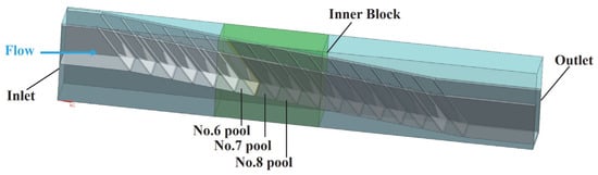
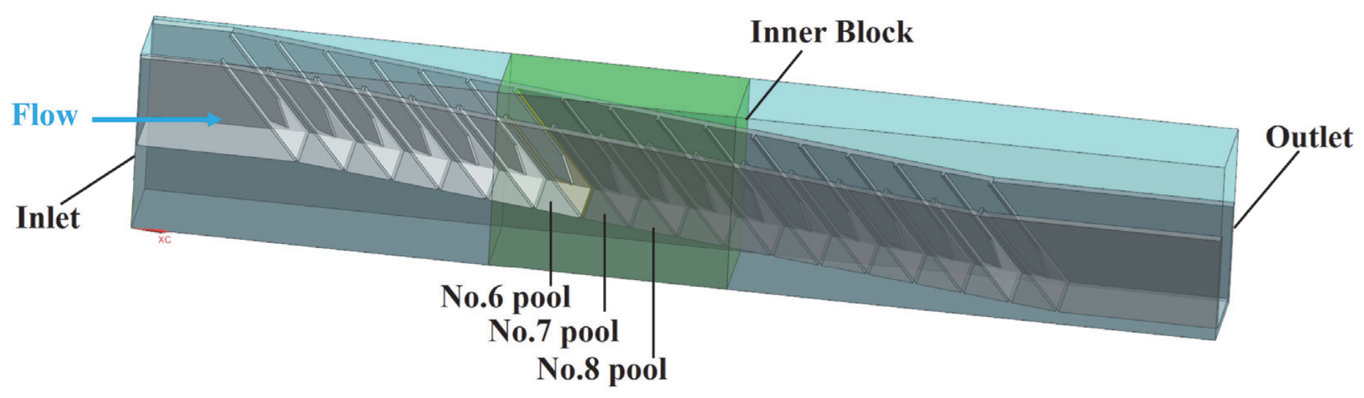
To optimize the balance between computational efficiency and the resolution of complex turbulent structures, a nested grid refinement strategy was implemented within the STAR-CCM+ environment. The Trimmed Cell Mesher was employed to generate a high-quality, hexahedral-dominant mesh, which is essential for capturing the sharp geometric gradients of the Denil baffles. As illustrated in Figure 3, a localized high-density refinement zone, the “Inner Block” (green), was established using Volumetric Controls, specifically encompassing the baffle notches where velocity gradients are most intense. This region utilized a characteristic cell size of $\mathsf{\Delta }x=2.0 \mathrm{c}\mathrm{m}$. To ensure numerical stability and minimize artificial dissipation at the refinement interfaces, a controlled surface growth rate was applied to facilitate a gradual mesh transition.

Figure 3. Schematic of computational domain mesh setup and boundary condition. The labeled No. 6–8 pools, within the fully developed flow region, serve as the representative pools for the subsequent hydrodynamic analyses.

Boundary conditions were configured to strictly adhere to hydraulic physical model specifications. The inlet was defined as a mass flow inlet, delivering a uniform mass flux corresponding to the designated discharge Q for each scenario, while the outlet was set as a pressure outlet with a hydrostatic pressure profile to facilitate stabilized free-surface discharge. Standard atmospheric pressure was applied to the top of the air phase, and the channel bed, side walls, and baffles were modeled as no-slip walls, consistent with common practice in fishway CFD studies [27,28]. It should be noted that real fishway surfaces (e.g., concrete or timber) are rougher than the modeled smooth walls, and this simplification may slightly overestimate near-bed velocity magnitudes. However, since an identical wall condition is applied to all three baffle configurations, the relative inter-configuration differences that underpin our conclusions are expected to remain robust. Under these numerical constraints, a cross-test matrix involving three baffle configurations and three representative flow rates ($Q_1=0.014 {\mathrm{m}}^3/\mathrm{s}$, $Q_2=0.058 {\mathrm{m}}^3/\mathrm{s}$, $Q_3=0.127 {\mathrm{m}}^3/\mathrm{s}$) was designed. This resulting set of nine core test cases (as detailed in Table 2) covers the typical operating window of Denil fishways, ranging from low-flow bottlenecks to high-flow hydraulic capacity limits. The two additional discharge cases (Q = 0.034 and 0.089 m³/s) were simulated only for the TDF configuration to extend the validation envelope against Odeh’s experimental head–discharge data [16].

Table 2. Simulation cases for the three baffle configurations. (Note: S and S₀ are defined in Figure 1, and Q denotes the discharge.).

Models	S (m)	S0	Q (m3/s)	Additional Cases
TDF	0.3	0.1	0.014, 0.058, 0.127	0.034, 0.089
SCDF	0.3	0.1	0.014, 0.058, 0.127	--
RDF	0.3	0.1	0.014, 0.058, 0.127	--

2.2.3. Model Validation

Grid independence was verified using three hydrodynamic indicators. The outlet velocity, computed as the area-averaged streamwise velocity over the downstream outlet cross-section, characterizes the overall flow through the domain. The near-bed streamwise velocity and near-bed TKE are extracted at a near-bed monitoring point within the 7th pool (in the fully developed region) at $z/d=0.10$ (i.e., 10% of the local flow depth above the bed) and at $x/S=0.5$ along the channel centerline, characterizing the near-bed flow that is central to the present study. As shown in Table 3, all three indicators converge monotonically with mesh refinement. The near-bed TKE is the most mesh-sensitive, decreasing markedly on coarse meshes (from 0.091 to 0.048 J/kg between Scheme 1 and Scheme 3) before stabilizing from Scheme 4 onward. The relative differences between Scheme 4 (≈2.47 × 10⁶ cells) and the finest Scheme 5 are 0.32%, <0.1%, and 2.4% for the three indicators, respectively, indicating that the solution is grid-independent at the resolution of Scheme 4. Scheme 4 was therefore adopted as the final mesh, providing grid-independent solutions at substantially reduced computational cost compared with Scheme 5.

Table 3. Mesh convergence study for five mesh schemes (TDF, Q₂ = 0.058 m³/s).

Mesh	Cell Counts	Main Block Size (cm)	Inner Block Size (cm)	Outlet Velocity (m/s)	Near-Bed Velocity (m/s)	Near-Bed TKE (J/kg)
Scheme 1	435,580	25	2	0.667	0.189	0.091
Scheme 2	707,807	20	2	0.644	0.184	0.057
Scheme 3	1,394,322	15	2	0.631	0.179	0.048
Scheme 4	2,471,862	10	2	0.620	0.178	0.042
Scheme 5	4,532,456	5	2	0.618	0.178	0.041

The numerical model was validated against the experimental data reported by Odeh [16]. Two parameters were selected to characterize the TDF’s hydrodynamic performance: the head–discharge relationship ($h_u$-$Q$) and the dimensionless discharge coefficient ($C_d$-$h_u/b$). The $h_u$-$Q$ relationship serves as a macroscopic hydraulic signature, reflecting the equilibrium between discharge input and structural flow resistance. Meanwhile, the dimensionless coefficient $C_d$ (normalized by $h_u$-$Q$) provides a robust measure of energy dissipation and hydraulic efficiency, isolating hydrodynamic characteristics from scale-dependent effects. As shown in Table 4, numerical results align well with experimental data, with relative errors within ±5% for all tested conditions, confirming the model’s fidelity in capturing the complex flow dynamics of Denil fishways.

Table 4. Comparison between numerical and experimental results for upstream flow depth and discharge coefficient across five discharge conditions.

Item	Q (m3/s)	Experimental Results	Present Study Results	Relative Error
$h_u$-$Q$	0.014	0.141	0.139	−1.42%
	0.034	0.222	0.214	−3.60%
	0.058	0.291	0.287	−1.37%
	0.089	0.372	0.354	−4.84%
	0.127	0.460	0.453	−1.52%
$C_d$-$h_u/b$	0.014	0.995	1.021	2.61%
	0.034	1.043	1.091	4.60%
	0.058	1.091	1.110	1.74%
	0.089	1.118	1.165	4.20%
	0.127	1.084	1.115	2.86%

Although the TDF, SCDF, and RDF exhibit distinct baffle profiles, they share an identical fundamental fluid–structure coupling mechanism for open-channel flow past rigid vertical baffles, with consistent governing equations and near-wall turbulence physics. The RNG $k-\epsilon$ model, verified to accurately capture boundary-layer separation and high-curvature shear layers in this flow regime, ensures consistent numerical accuracy across all three geometric configurations. This study only provides independent experimental validation for the benchmark TDF configuration, while the SCDF and RDF lack dedicated experimental or high-fidelity Large Eddy Simulation (LES) validation. This limitation may introduce minor uncertainties in the absolute values of near-bed hydrodynamic predictions. However, all key conclusions are derived from relative differences between the three baffle configurations, rather than absolute numerical values, so the core findings regarding geometric effects and layered hydrodynamic regulation remain reasonably supported within the tested conditions.

2.3. Layered Hydrodynamic Evaluation Framework

Previous studies have extensively demonstrated that a characteristic vertical dual-flow regime is inherently induced within Denil fishways: the upper layer is dominated by a forward high-speed jet, while the lower layer is occupied by large-scale reverse recirculation [18,20]. To accurately capture the distinct hydrodynamic responses of these two functional regions to bottom geometry variations, this study adopts a layered evaluation framework rather than a bulk cross-sectional analysis. Similar layered flow topologies, in which a jet-dominated layer coexists with large-scale recirculation zones, have been systematically characterized in vertical-slot and pool-weir fishways using both Acoustic Doppler Velocimeter (ADV) measurements and CFD analyses [29,30].

Theoretically, the geometric area-equivalent height ($h_{geo}=A/W$) could serve as the stratification boundary. However, using $h_{geo}$ directly tends to place the partition too high because the downward momentum transfer of the main jet extends the effective baffle-controlled zone above the purely geometric level [16,23]. Furthermore, under low-discharge conditions $h_{geo}$ approaches the free surface, rendering a purely geometric partition physically unrepresentative. To account for these hydrodynamic realities, an effective area-equivalent blocking height ($h_{eq}$) is defined as an empirically corrected layered reference:

$$h_{eq}=\eta {\displaystyle \frac{A}{W}}$$

(3)

where $A$ denotes the actual wetted baffle area, $W$ is the channel width, and $\eta$ is introduced as a dimensionless empirical correction coefficient ($0 < \eta \le 1$).

Based on this empirically calibrated layered reference, the spatial mean velocity and mean TKE were extracted separately for each layer to quantitatively assess macroscopic energy redistribution. TKE is selected as the primary turbulence indicator in this study due to its well-established ecological relevance and widespread adoption in fishway hydrodynamic assessments [29,31]. Unlike local shear or instantaneous dissipation rate, TKE provides a spatially integrated measure of turbulent fluctuation intensity, which directly reflects the flow disturbance level encountered by fish during migration. For weak-swimming and benthic species, elevated TKE increases swimming energy consumption, reduces postural stability, and narrows the usable low-turbulence resting zone. In the present layered evaluation framework, TKE enables clear discrimination between the high-turbulence upper jet layer and the near-bed low-energy layer, making it an appropriate metric to quantify habitat suitability improvements induced by baffle geometry modifications. It should be noted that TKE characterizes the overall intensity of turbulent fluctuations but not the coherence of turbulent structures, which some fish can exploit for efficient swimming (e.g., the Kármán gait) [32,33]. The corresponding integral expressions are defined as follows:

$${\overline{u}}_i={\displaystyle \frac{1}{A_i}}{{\displaystyle \iint }}_{z\in {\mathsf{\Omega }}_i}udA \left(i=lower,upper\right)$$

(4)

$${\overline{TKE}}_i={\displaystyle \frac{1}{A_i}}{{\displaystyle \iint }}_{z\in {\mathsf{\Omega }}_i}kdA (i=lower,upper)$$

(5)

where $u$ denotes the streamwise velocity component (positive downstream), $A_i$ represents the wetted cross-sectional area of the respective layer, and $k$ denotes the turbulent kinetic energy. The integration domains ${\mathsf{\Omega }}_{lower}$ ($z\le h_{eq}$) and ${\mathsf{\Omega }}_{upper}$ ($z>h_{eq}$) correspond to the physically calibrated lower and upper layers, respectively. Here, the streamwise velocity is adopted as the primary kinematic indicator, as it directly governs the drag encountered by fish during upstream migration and is the standard velocity metric in fishway hydrodynamic assessments [19,20]. In the analysis sections that follow, ‘near-bed’ indicators refer to area-weighted averages over the lower flow layer ($z\le h_{eq}$) defined by this layered framework, distinct from the single near-bed monitoring point ($z/d=0.10$) used for mesh-independence verification in Section 2.2.3.

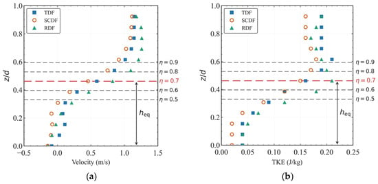
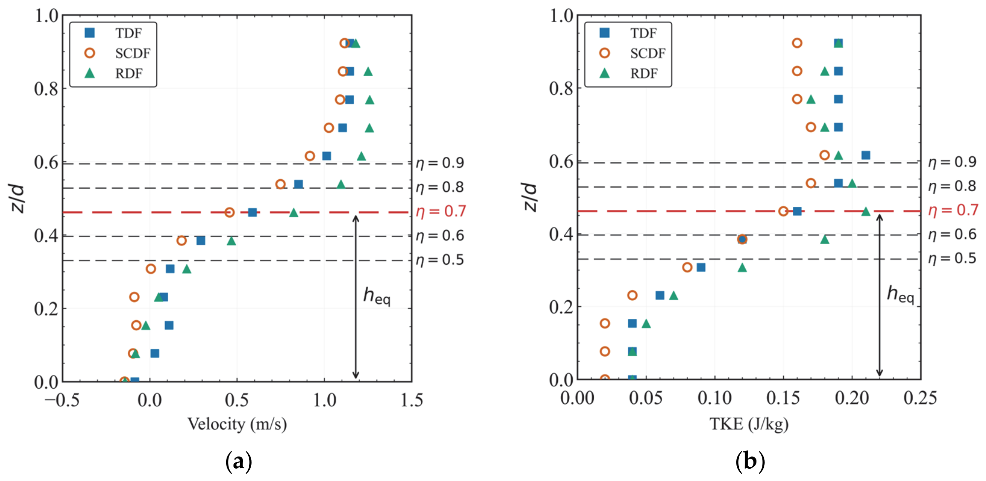
The boundary parameter $\eta$, which separates the upper and lower layers in this framework, is not prescribed arbitrarily but calibrated from the flow-field characteristics of the present simulations. As shown in Figure 4, the vertical profiles of velocity and TKE along Axis B under intermediate discharge (Q₂) are examined for five candidate boundaries ($\eta$ = 0.5, 0.6, 0.7, 0.8, 0.9). The velocity profiles show a clear vertical variation, with higher velocities in the upper region and lower velocities in the lower region. The $\eta =0.7$ line consistently coincides with the transition between these two regions across all three configurations. This selection is further corroborated by the TKE profiles, in which $\eta =0.7$ corresponds to the boundary between the lower low-TKE region and the upper high-TKE region. Boundaries with $\eta \le 0.6$ fall within the low-velocity lower region, while $\eta \ge 0.8$ falls within the high-velocity upper region, both of which would obscure the distinct hydrodynamic characteristics of each layer. The value $\eta =0.7$ is therefore adopted for the present study. A sensitivity analysis of the four layered indicators at $\eta$ = 0.6, 0.7, and 0.8 is reported in the Supplementary Material (Table S1). The results show that the main qualitative trends are generally retained around the adopted value of η = 0.7, although minor reordering occurs for some lower-layer indicators at the bounds of the tested η range. It should be noted that this parameter is determined based on the local flow-field characteristics and may vary with baffle spacing, bed slope, and discharge conditions. Thus, its value should be calibrated accordingly in applications involving different geometric or hydraulic parameters.

Figure 4. Vertical profiles of (a) velocity and (b) TKE along Axis B ($y=0.5W$) under intermediate discharge (Q₂) for the three baffle configurations, with horizontal lines indicating five candidate boundaries (η = 0.5, 0.6, 0.7, 0.8, 0.9). The red dashed line denotes the adopted effective blocking height ($\eta =0.7$).

3. Results and Discussion

The presentation of results is organized as follows. Section 3.1 and Section 3.2 compare the velocity and TKE fields among the three configurations at the intermediate design discharge $Q_2$. Section 3.3 then extends the comparison across three discharges ($Q_1$, $Q_2$, $Q_3$) using layer-averaged indicators. Section 3.4 synthesizes the findings and discusses their implications for fishway design.

3.1. Flow Field Structure in Longitudinal and Cross-Sections

To examine the flow field characteristics, the central longitudinal section and a representative cross-section within the fully developed flow region were extracted for analysis. The following subsections evaluate how the cross-sectional geometry of the bottom baffle affects the distribution of the velocity field and TKE in the longitudinal and transverse directions.

3.1.1. Velocity and TKE Distribution in the Longitudinal Section

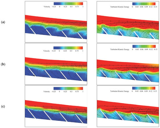
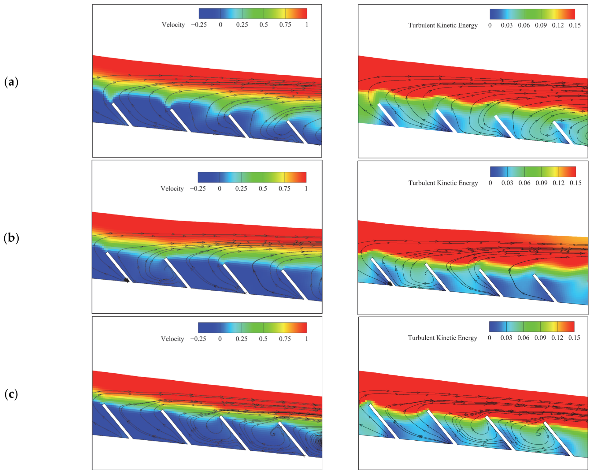
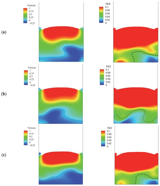
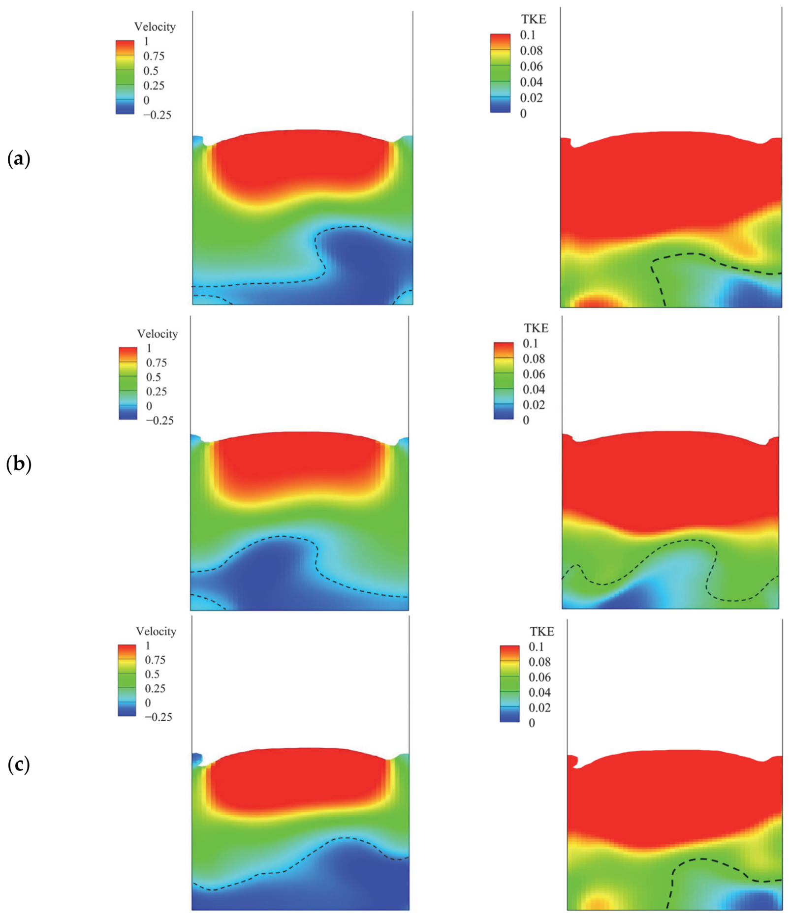
Figure 5 presents the streamwise velocity component and TKE contours at the central longitudinal section within the fully developed region. The inter-configuration comparisons in this section are based on the 7th pool, which is taken as the representative pool within this region. The flow field shows a clear vertical layering pattern, with different characteristics in the upper and lower layers. In the upper jet-dominated layer, the three configurations show comparable patterns in both velocity and TKE distributions. In the lower baffle-controlled layer, the flow fields of the three configurations exhibit observable inter-configuration differences. In the TDF, positive streamwise velocity extends to a lower vertical position within the lower layer, and the high-TKE region similarly extends closer to the channel bed, leaving a relatively narrow reverse-flow zone near the bed. In the SCDF, the reverse-flow zone in the lower layer is larger than in the TDF, with the high-TKE region more confined to the upper portion of the lower layer. In the RDF, the lower layer is dominated by reverse flow across most of its vertical extent, with the high-TKE region extending closest to the channel bed and the baffle among the three configurations. These contour maps indicate that the inter-configuration differences in the spatial flow structure are primarily concentrated in the lower layer, with the upper layer showing comparable patterns across all configurations. Some variation between successive pools is also observable in Figure 5; the magnitude of this variation, as well as its relation to the inter-configuration differences identified above, is examined in Section 3.3.

Figure 5. Contour maps of streamwise velocity component (left, m/s) and turbulent kinetic energy (right, J/kg) at the central longitudinal section within the fully developed region (pools 6–8) under the intermediate discharge ($Q_2=0.058 {\mathrm{m}}^3/\mathrm{s}$, for the three baffle configurations: (a) TDF; (b) SCDF; (c) RDF.

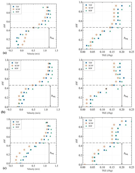
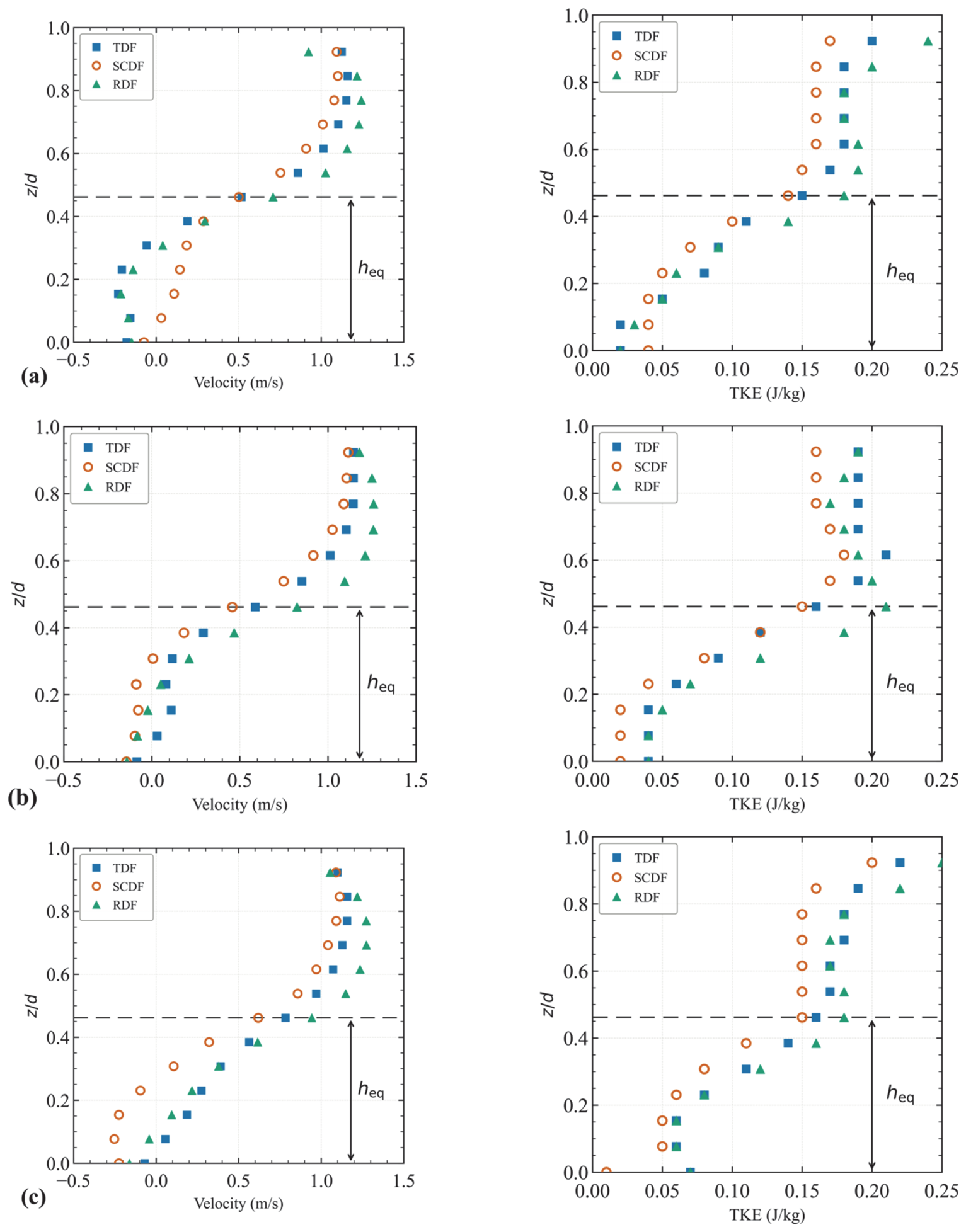
Figure 6 presents the velocity and TKE profiles along three vertical measurement axes (A, B, C) at the central cross-section of the 7th pool, providing a more detailed view of the vertical flow distribution. In the upper layer (${z/d>h}_{eq}$), the velocity and TKE profiles of the three configurations overlap closely, consistent with the small inter-configuration differences observed in the upper-layer indicators. In the lower layer (${z/d<h}_{eq}$), inter-configuration differences are observed across all three axes, though the specific patterns differ among axes. At axis A, the SCDF maintains positive near-bed velocity while the TDF and RDF show comparable reverse flow; near-bed TKE values are similar across the three configurations. At axis B, the TDF maintains positive near-bed velocity while the SCDF and RDF show comparable reverse flow, and the SCDF shows the lowest near-bed TKE. At axis C, the SCDF shows the strongest reverse flow while the TDF and RDF show comparable and notably weaker reverse flow; the near-bed TKE values of the TDF and RDF are comparable and both exceed those of the SCDF. Notably, the near-bed velocity of the SCDF shifts from positive flow at axis A to the strongest reverse flow at axis C, indicating a pronounced lateral variation in the near-bed flow characteristics of the SCDF across the channel width. These profile observations are in general agreement with the contour map results in Figure 5, further indicating that the influence of baffle base geometry is mainly concentrated in the lower layer.

Figure 6. Vertical profiles of velocity (left, m/s) and TKE (right, J/kg) along axes A, B, and C at the central cross-section of the 7th pool for Q₂: (a) y = 0.2W; (b) y = 0.5W; (c) y = 0.8W. The dashed line denotes $h_{eq}$.

3.1.2. Velocity and TKE Distribution in the Cross Section

Figure 7 presents the cross-sectional contour maps of streamwise velocity and TKE for the three baffle configurations at the central cross-section of the 7th pool under $Q_2$. The upper layer shows high streamwise velocity and high TKE across the three configurations, while the lower layer exhibits visible inter-configuration variation in both velocity and TKE distributions. To quantify these features, the proportion of the lower-layer cross-sectional area occupied by reverse flow (streamwise velocity < 0 m/s) and the proportion with TKE below 0.05 J/kg (the value reported by Silva et al. [31] for cyprinid near-bed habitat preference) were computed for each configuration. The maximum inter-configuration difference in the reverse-flow proportion is approximately 8 percentage points (between the TDF and the RDF). For the low-TKE proportion, the TDF and the RDF differ by less than 2 percentage points, while the SCDF exceeds the TDF and the RDF by approximately 10 and 12 percentage points, respectively. Furthermore, lateral non-uniformity in the near-bed flow is observed in all three configurations, with the lateral variation in the reverse-flow pattern most pronounced in the SCDF.

Figure 7. Cross-sectional contour maps of streamwise velocity (left, m/s) and TKE (right, J/kg) at the central cross-section of the 7th pool under $Q_2$ for the three baffle configurations: (a) TDF; (b) SCDF; (c) RDF. The black dashed lines mark the boundaries of the reverse-flow region (streamwise velocity = 0) and the low-TKE region (TKE = 0.05 J/kg).

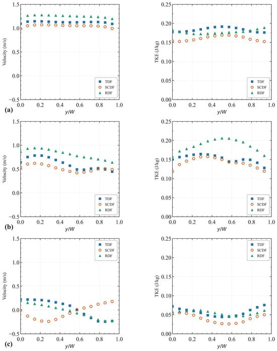
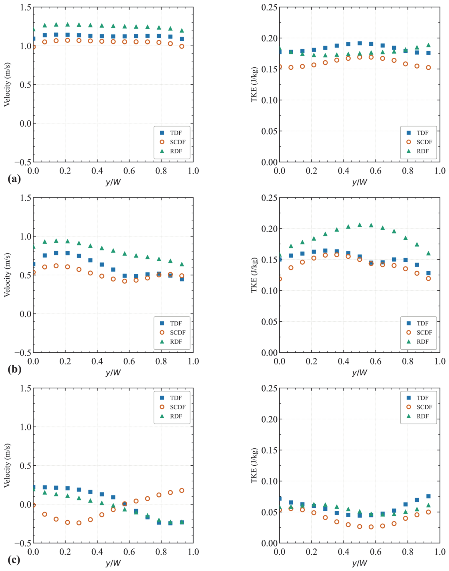
Figure 8 presents the transverse profiles of streamwise velocity and TKE at three representative depths (z/d = 0.75, 0.50, 0.25) within the 7th pool. At z/d = 0.75 (upper layer), the profiles of the three configurations overlap closely in both streamwise velocity and TKE. At z/d = 0.50, the SCDF shows slightly lower velocity and TKE than the TDF and the RDF, while the TDF and RDF profiles remain comparable. At z/d = 0.25 (near-bed layer), two features are observed. First, the TKE profile of the SCDF lies below those of the TDF and the RDF across the channel width, indicating that the lower near-bed TKE of the SCDF extends across the entire channel section. Second, the near-bed streamwise velocity profiles show lateral asymmetry in all three configurations, with the lateral pattern of the SCDF differing from that of the TDF and the RDF. These observations indicate that the inter-configuration differences are concentrated in the near-bed layer.

Figure 8. Transverse profiles of streamwise velocity (left) and TKE (right) at three relative depths (Q₂): (a) z/d = 0.75; (b) z/d = 0.50; (c) z/d = 0.25.

3.2. Streamwise Evolution of Hydrodynamic Characteristics Within the Pool

3.2.1. Spatial Evolution of Velocity and TKE

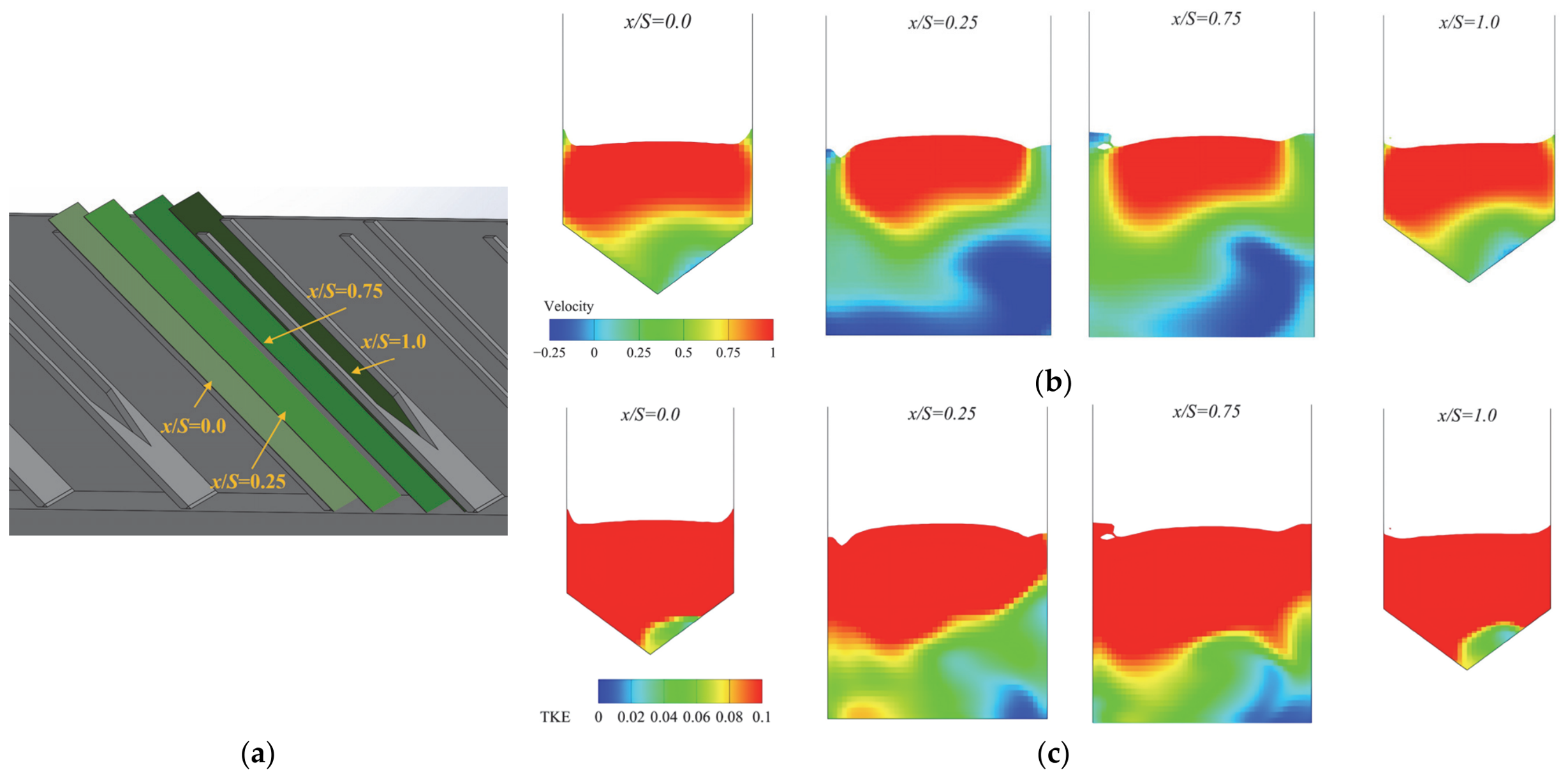
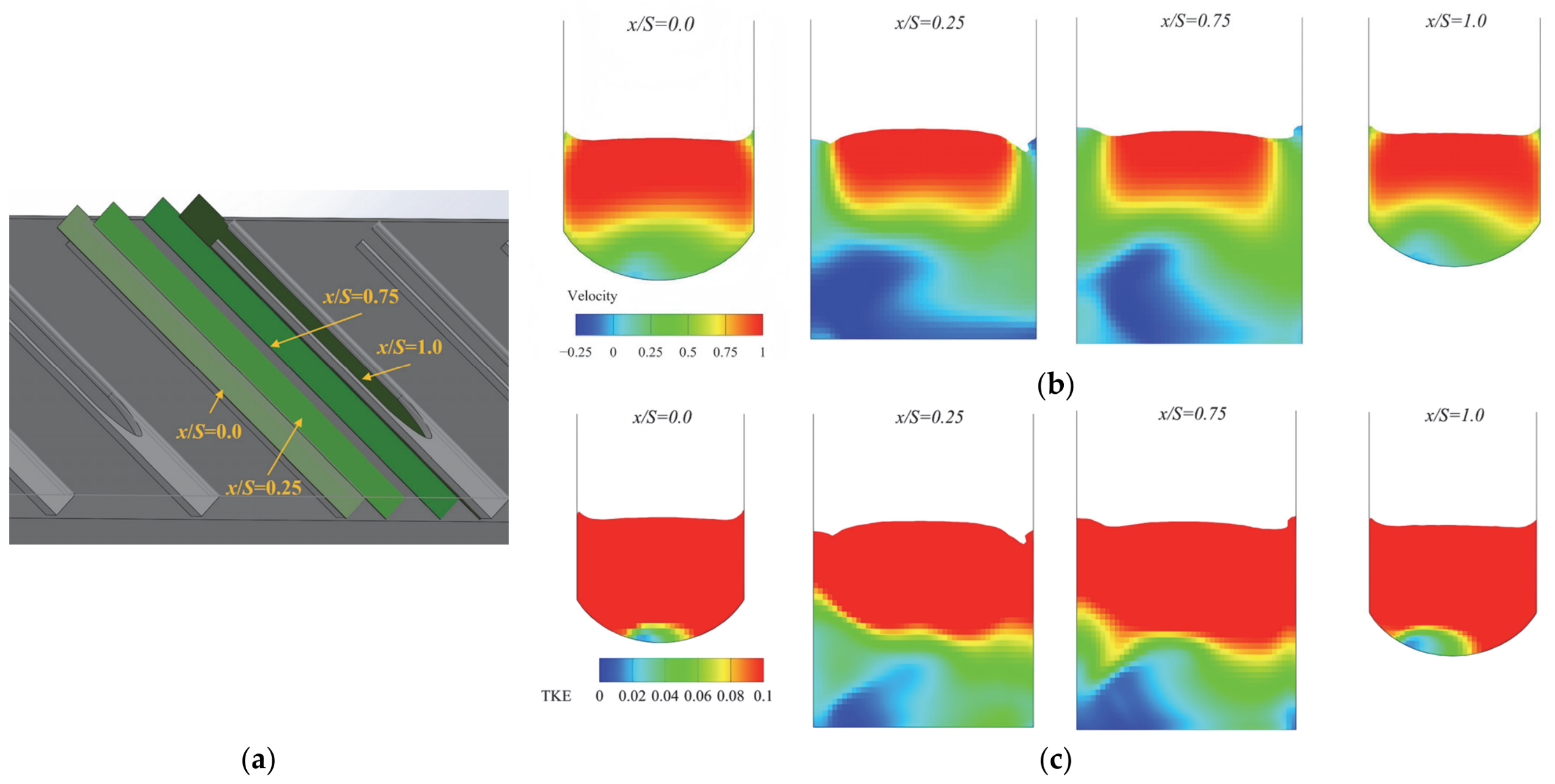
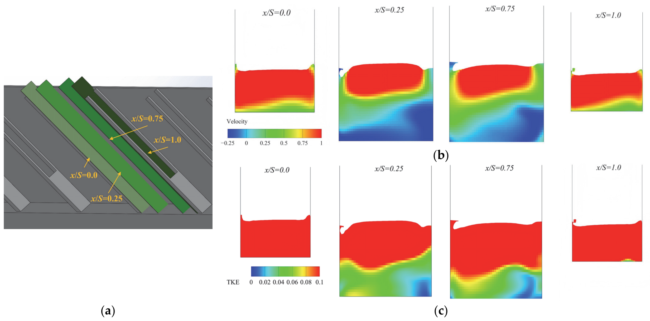
While Section 3.1 examined the time-averaged flow topology at characteristic cross-sections within the fully developed region, this section traces the streamwise spatial evolution of hydrodynamics within a single pool, spanning from the upstream baffle face ($x/S=0$) to the downstream baffle face ($x/S=1.0$). Figure 9, Figure 10 and Figure 11 present sequential velocity and TKE contour maps at four representative dimensionless positions ($x/S=0,0.25,0.75,1.0$) for the three configurations.

Figure 9. The flow field within a single pool for the TDF configuration. (a) Isometric view with cross-section locations (x/S = 0, 0.25, 0.75, 1.0); (b) Sequential contour maps of streamwise velocity component; (c) Sequential contour maps of TKE.

Figure 10. The flow field within a single pool for the SCDF configuration. (a) Isometric view with cross-section locations (x/S = 0, 0.25, 0.75, 1.0); (b) Sequential contour maps of streamwise velocity component; (c) Sequential contour maps of TKE.

Figure 11. The flow field within a single pool for the RDF configuration. (a) Isometric view with cross-section locations (x/S = 0, 0.25, 0.75, 1.0); (b) Sequential contour maps of streamwise velocity component; (c) Sequential contour maps of TKE.

The flow field within the pool shows a consistent streamwise evolution pattern across all three configurations. At $x/S=0$, the lower layer shows a limited reverse-flow zone, with the shape of the near-bed low-velocity region determined by the baffle base geometry: a V-shaped distribution in the TDF, an arc-shaped distribution in the SCDF, and a horizontal band in the RDF. At $x/S=0.25$, the reverse-flow zone expands substantially, reaching its largest areal extent within the pool, while the high-TKE region remains largely confined to the upper layer. At $x/S=0.75$, positive-velocity fluid from the upper layer extends to its lowest vertical position, reducing the areal extent of the reverse-flow zone; correspondingly, the near-bed low-TKE region reaches its smallest extent at this location. At $x/S=1.0$, the lower layer recovers a limited reverse-flow zone with high TKE values comparable to those at $x/S=0$, consistent with the periodic nature of the fully developed flow in successive pool units.

Although the three configurations share the above general streamwise pattern, the bottom baffle geometry produces observable differences in the vertical extent of the positive-velocity region and the size of the near-bed low-TKE zone. In the TDF, positive-velocity fluid extends to a lower vertical position at $x/S=0.25$ and $x/S=0.75$ than in the SCDF and RDF, and the lower layer shows pronounced lateral non-uniformity at all four streamwise positions. In the SCDF, the positive-velocity region is more vertically confined and the near-bed low-TKE zone is the largest among the three configurations, with more laterally uniform flow distributions. In the RDF, the positive-velocity region shows the least vertical extension into the lower layer, and the flow distributions are the most laterally uniform. These observations suggest that bottom baffle geometry can affect the vertical extent to which positive-velocity fluid extends into the lower layer under the intermediate discharge.

3.2.2. Streamwise Evolution of Layer-Averaged Velocity and TKE

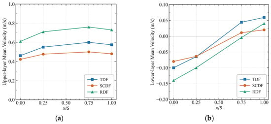
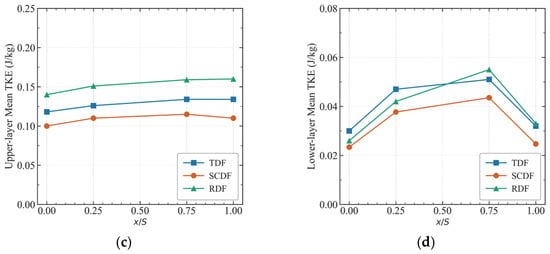
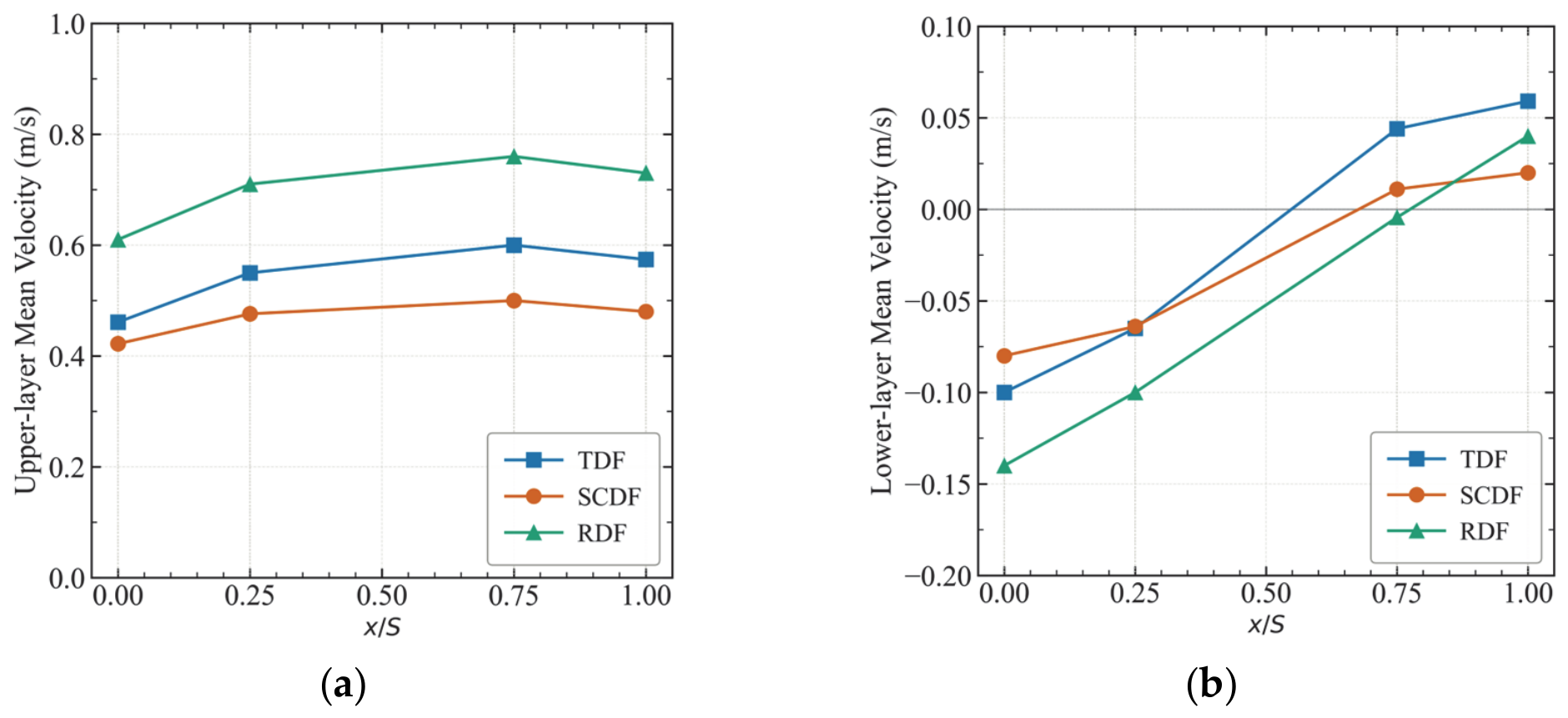
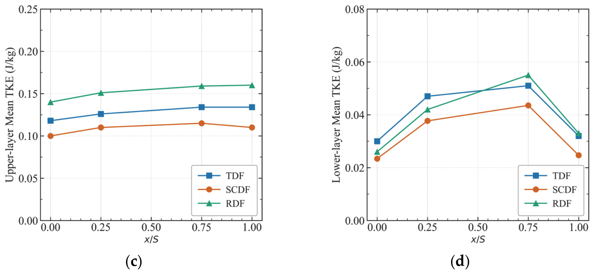
To quantitatively characterize the streamwise evolution of the layered flow field, Figure 12 presents the cross-sectional mean velocity and mean TKE profiles for both the upper and lower layers across the three configurations. The profiles are plotted against the dimensionless streamwise distance $x/S$.

Figure 12. The cross-sectionally averaged hydrodynamic metrics along longitudinal distance ($x/S$) for the three baffle configurations. (a) Upper-layer mean velocity; (b) Lower-layer mean velocity; (c) Upper-layer mean TKE; (d) Lower-layer mean TKE.

The flow field within the pool shows a broadly similar streamwise evolution across all three configurations. In the upper layer, both velocity and TKE increase with $x/S$, reaching their highest values at approximately $x/S=0.75$. In the lower layer, the streamwise velocity transitions from negative values near $x/S=0$ to positive values near $x/S=1.0$, with the zero-crossing occurring in the $x/S=0.5-0.75$ range. The lower-layer TKE reaches its peak at approximately $x/S=0.75$ and declines sharply at $x/S=1.0$, returning to levels comparable to those at $x/S=0$. This general streamwise pattern is observed in all three baffle configurations, reflecting the periodic nature of the fully developed flow within successive pool units.

The three configurations differ in both layers, but inter-configuration differences are more evident in the lower layer. In the upper layer, the RDF shows the highest velocity and TKE values at all streamwise positions, followed by the TDF and then the SCDF. In the lower layer, the RDF shows the largest reverse-flow magnitude at $x/S=0$, followed by the TDF and then the SCDF. Notably, by $x/S=0.75$, the TDF shows the highest positive velocity in the lower layer while the RDF remains close to zero, indicating that the streamwise position of the velocity reversal differs among configurations. The lower-layer TKE shows clear inter-configuration differences: the SCDF maintains the lowest values at all streamwise positions, while the TDF and RDF show comparable and higher peak values at $x/S\approx 0.75$. These results suggest that bottom baffle geometry affects the streamwise evolution of the layered flow field, with more pronounced differences occurring in the lower layer, particularly in TKE.

Note that the metrics reported here are streamwise-local layer averages under the intermediate discharge Q2; the pool-averaged indicators in Section 3.3 integrate over all streamwise positions and across the full discharge range.

3.3. Layered Assessment of Baffle Configuration Effects

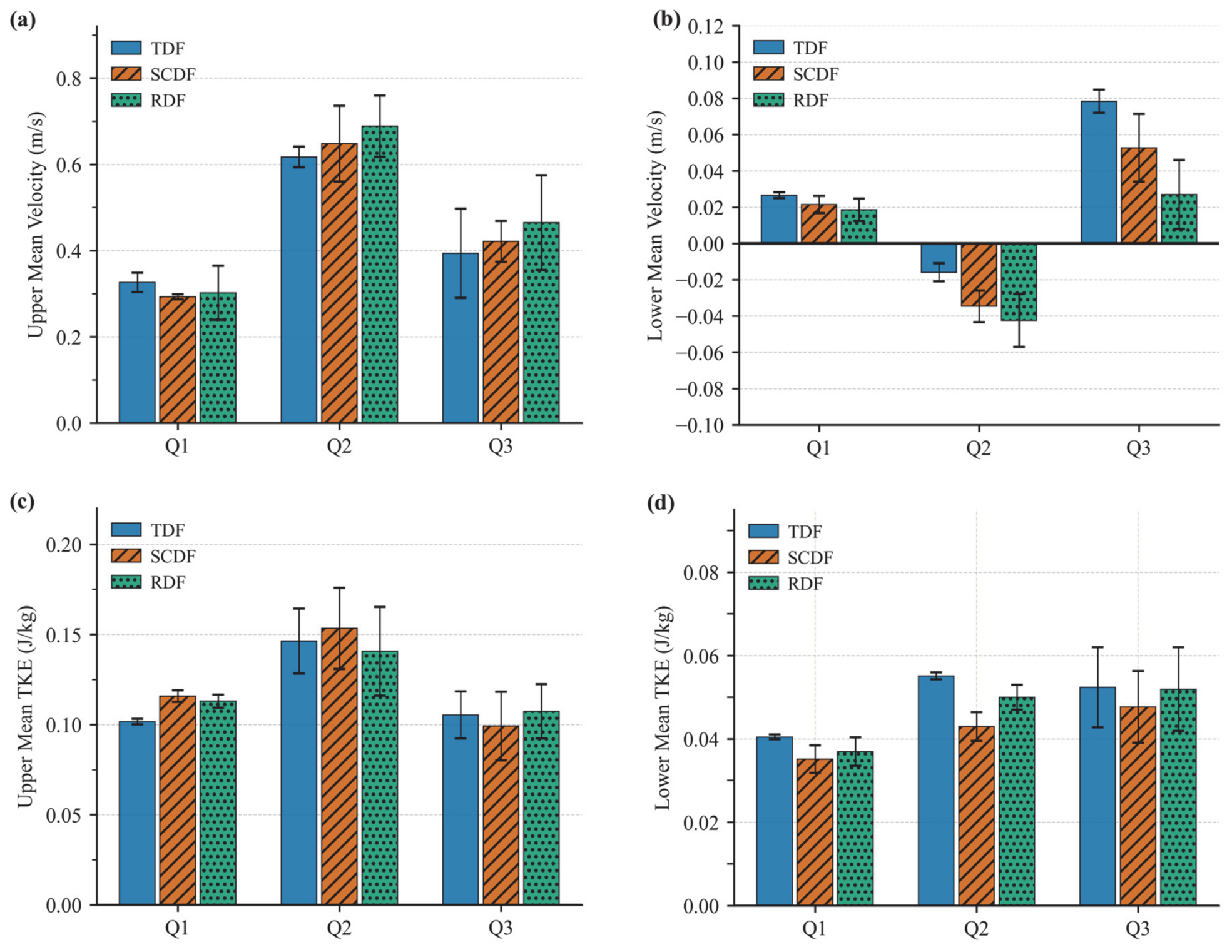
This section extends the configuration comparison from $Q_2$ to the full discharge range ($Q_1$, $Q_2$, $Q_3$) to examine whether the configuration-related trends observed under $Q_2$ are retained across the tested discharge range. Figure 13 presents the four layered hydrodynamic indicators (upper and lower mean velocity and TKE) across the three discharges for all three configurations; each data point represents the mean over three successive pools in the fully developed region (the 6th, 7th, and 8th), with error bars representing the pool-to-pool standard deviation.

Figure 13. Layered hydrodynamic indicators across three discharge conditions for three baffle configurations. (a) Upper-layer cross-sectional mean velocity; (b) Lower-layer cross-sectional mean velocity; (c) Upper-layer cross-sectional mean turbulent kinetic energy; (d) Lower-layer cross-sectional mean turbulent kinetic energy. Each data point represents the mean over three successive pools in the fully developed region (the 6th, 7th, and 8th pools), and the error bars represent the pool-to-pool standard deviation.

The upper-layer indicators in Figure 13a,c show small inter-configuration differences in both velocity and TKE across all three discharges, of magnitudes comparable to or within the pool-to-pool variability. The macroscopic conveyance capacity of the upper layer therefore remains functionally consistent across configurations and discharges. This consistency confirms that the equivalent openness ratio constraint effectively prevents area-effect interference, in contrast to the substantial variation in macroscopic discharge capacity reported when the openness ratio is not constrained [23], and supports a more controlled comparison in which the observed lower-layer differences can be interpreted primarily in relation to baffle geometry, rather than to differences in openness ratio.

Figure 13b shows that the lower-layer mean velocity follows a consistent inter-configuration pattern across the discharge range. Under low discharge ($Q_1$), all three configurations yield small positive values, with the TDF the highest and the RDF the lowest. Under intermediate discharge ($Q_2$), the values become negative as the macro-scale recirculation in the lower layer fully develops; the reverse-flow magnitude follows the inverse order, with the RDF showing the strongest reverse flow and the TDF the weakest. Under high discharge ($Q_3$), the values return to positive but again rank in the same order, with the TDF the highest and the RDF the lowest. The SCDF and RDF therefore consistently reduce the lower-layer mean velocity relative to the TDF baseline under $Q_1$ and $Q_3$, and produce more pronounced reverse flow under $Q_2$, indicating a configuration-related modification of the near-bed flow field within the tested discharge range. The RDF exhibits a more pronounced effect than the SCDF on the lower-layer mean velocity across the three discharges.

A similar inter-configuration pattern, though of smaller magnitude, is observed for the lower-layer mean TKE in Figure 13d. Under $Q_2$, the TDF shows the highest value and the SCDF the lowest, with the RDF being intermediate; the difference between the TDF and the SCDF, approximately 22%, exceeds the pool-to-pool variability of either configuration, while the difference between the TDF and the RDF is comparable to the pool-to-pool variability. Under $Q_1$, the inter-configuration differences are small and barely exceed the variability, with the SCDF showing a slightly larger reduction than the RDF. Under $Q_3$, the three configurations yield comparable values, and the inter-configuration differences fall within the pool-to-pool variability. The SCDF and RDF therefore both reduce the lower-layer TKE relative to the TDF baseline across the tested discharge range, with the SCDF achieving the larger reduction at all three discharges.

The above results allow the inter-configuration differences to be assessed against the pool-to-pool variability of the flow. The pool-to-pool variability, reflected in the error bars of Figure 13, is observed to increase with discharge across all three configurations. This trend is consistent with the general physical expectation that the spatial variability of the flow between successive pools increases with the mean flow magnitude. However, the specific physical mechanisms, which may involve enhanced non-stationary characteristics at higher discharges, are beyond the scope of the present steady-state analysis. For the lower-layer mean velocity, the inter-configuration ranking remains consistent across the three discharges, and the magnitude of the inter-configuration differences exceeds the pool-to-pool variability under $Q_1$ and is of comparable magnitude under $Q_2$ and $Q_3$. For the lower-layer TKE, the inter-configuration differences exceed the pool-to-pool variability under $Q_1$ and $Q_2$ for the TDF-SCDF comparison, while all inter-configuration differences under $Q_3$ lie within the variability range.

3.4. Discussion

Based on the layered assessment in Section 3.3, the inter-configuration differences in the lower baffle-controlled layer may inform design considerations for Denil fishways targeting weak-swimming and benthic species. The maximum relative difference in pool-averaged lower-layer TKE between the TDF and the SCDF, approximately 22%, occurs under intermediate discharge, with lower-layer TKE values of approximately 0.055, 0.043, and 0.050 J/kg for the TDF, SCDF, and RDF, respectively. These values are directly comparable to the thresholds reported for cyprinid fishes: in an experimental pool-type fishway, Silva et al. [31] found that Iberian barbel (a cyprinid) preferentially occupied near-bed regions with TKE below approximately 0.05 J/kg, spending significantly less time in higher-TKE zones. Consistently, Lupandin [34] reported that the critical swimming speed of perch declined once turbulence exceeded a body-length-dependent threshold, with smaller individuals affected at lower turbulence levels. As the configurations examined here differ in lower-layer TKE around this ecologically relevant range, baffle geometry may modulate the suitability of the near-bed resting zone for small-bodied, weak-swimming fish, although the precise behavioral response remains to be confirmed through species-specific studies.

These findings provide preliminary hydraulic references for site-specific baffle selection, with the overarching goal of improving near-bed hydraulic conditions for weak-swimming and benthic species. The RDF may be preferable for sites where expanding the near-bed reverse-flow refuge zone is the primary objective, given its largest reverse-flow area under these conditions. The SCDF may be preferable for sites where minimizing near-bed turbulence is the primary objective, given its lowest lower-layer TKE across the tested discharge range. The TDF remains a relevant baseline for sites targeting strong-swimming species. The above recommendations are based on the tested discharge range; the inter-configuration ranking outside this range remains to be confirmed by further investigation.

It should be noted that the present analysis has several limitations. The detailed three-dimensional comparisons of velocity and TKE fields are based on the intermediate discharge $Q_2$, while the cross-discharge comparison is summarized through four layer-averaged indicators in Figure 13; detailed three-dimensional comparisons across all tested discharges, as well as under operating conditions beyond the tested range, are beyond the scope of the present study. Furthermore, the hydraulic improvements demonstrated here do not translate directly into proportional gains in passage efficiency, and the present CFD analysis cannot resolve whether the observed inter-configuration differences are sufficient to produce measurable biological outcomes. Passage success is governed by multiple interacting factors beyond hydrodynamics, including fish behavior, motivation, and individual variation in swimming capacity, and turbulence is not uniformly detrimental, as some fish exploit coherent turbulent structures (e.g., the Kármán gait) to reduce swimming costs [32,33], so that lower near-bed TKE does not invariably equate to improved passage conditions. Field or flume-based passage trials with representative weak-swimming and benthic species are identified as a necessary next step to establish the linkage between hydraulic conditions and biological outcomes.

4. Conclusions

This study indicates that, under a unified openness ratio constraint, the cross-sectional geometry of baffles exerts its primary hydrodynamic regulation effect on the lower baffle-controlled layer of Denil fishways, while the macroscopic conveyance capacity of the upper layer remains functionally consistent across configurations. By enforcing a unified openness ratio for three bottom configurations, the area effect was decoupled from the shape effect, enabling systematic isolation of the geometric regulation mechanism. The main findings are summarized as follows:

• The geometric variations primarily regulate the lower baffle-controlled layer, with only small differences observed in the upper jet-dominated zone. The macroscopic conveyance capacity and the core function of the upper fast-swimming passage are preserved across the tested discharge range.
• The conventional V-shaped baffle (TDF) generally shows higher lower-layer TKE than the modified configurations, although the inter-configuration TKE differences fall within the pool-to-pool variability under high discharge.
• The rectangular baffle (RDF) produces the largest near-bed reverse-flow zone under intermediate discharge, with the lowest lower-layer mean velocity at low and high discharges among the three configurations.
• The U-shaped baffle (SCDF) generally shows lower lower-layer TKE, particularly under low and intermediate discharges, but this trend becomes less distinguishable under high discharge.

Building upon these mechanistic findings, future research will extend to more complex practical engineering conditions, including variable bed slopes, fluctuating water levels, and multi-flow regimes. The pool-to-pool variability of the near-bed flow indicators is observed to increase with discharge, and the underlying mechanism warrants further investigation using non-stationary methods such as URANS or LES. A systematic assessment of how the choice of representative pool affects spatially detailed inter-configuration comparisons would further strengthen the methodological basis. In addition, coupling hydraulic performance metrics with species-specific ecological suitability indicators through optimization algorithms may provide a pathway toward globally optimized baffle geometries.

References

- Nilsson, C.; Reidy, C.A.; Dynesius, M.; Revenga, C. Fragmentation and Flow Regulation of the World’s Large River Systems. Science 2005, 308, 405–408. [Google Scholar] [CrossRef] [Scilit]
- Belletti, B.; Garcia de Leaniz, C.; Jones, J.; Bizzi, S.; Börger, L.; Segura, G.; Castelletti, A.; van de Bund, W.; Aarestrup, K.; Barry, J.; et al. More than One Million Barriers Fragment Europe’s Rivers. Nature 2020, 588, 436–441. [Google Scholar] [CrossRef] [Scilit] [PubMed]
- Grill, G.; Lehner, B.; Thieme, M.; Geenen, B.; Tickner, D.; Antonelli, F.; Babu, S.; Borrelli, P.; Cheng, L.; Crochetiere, H.; et al. Mapping the World’s Free-Flowing Rivers. Nature 2019, 569, 215–221. [Google Scholar] [CrossRef] [Scilit] [PubMed]
- Chen, Q.; Li, Q.; Lin, Y.; Zhang, J.; Xia, J.; Ni, J.; Cooke, S.J.; Best, J.; He, S.; Feng, T.; et al. River Damming Impacts on Fish Habitat and Associated Conservation Measures. Rev. Geophys. 2023, 61, e2023RG000819. [Google Scholar] [CrossRef] [Scilit]
- Lucas, M.; Baras, E. Migration of Freshwater Fishes; Wiley-Blackwell: Oxford, UK, 2001. [Google Scholar]
- Poff, N.L.; Olden, J.D.; Merritt, D.M.; Pepin, D.M. Homogenization of Regional River Dynamics by Dams and Global Biodiversity Implications. Proc. Natl. Acad. Sci. USA 2007, 104, 5732–5737. [Google Scholar] [CrossRef] [Scilit]
- Barbarossa, V.; Schmitt, R.J.P.; Huijbregts, M.A.J.; Zarfl, C.; King, H.; Schipper, A.M. Impacts of Current and Future Large Dams on the Geographic Range Connectivity of Freshwater Fish Worldwide. Proc. Natl. Acad. Sci. USA 2020, 117, 3648–3655. [Google Scholar] [CrossRef] [Scilit]
- Katopodis, C.; Williams, J.G. The Development of Fish Passage Research in a Historical Context. Ecol. Eng. 2012, 48, 8–18. [Google Scholar] [CrossRef] [Scilit]
- Clay, C.H. Design of Fishways and Other Fish Facilities, 2nd ed.; CRC Press: Boca Raton, FL, USA, 2017. [Google Scholar]
- Noonan, M.J.; Grant, J.W.A.; Jackson, C.D. A Quantitative Assessment of Fish Passage Efficiency. Fish Fish. 2012, 13, 450–464. [Google Scholar] [CrossRef] [Scilit]
- Silva, A.T.; Lucas, M.C.; Castro-Santos, T.; Katopodis, C.; Baumgartner, L.J.; Thiem, J.D.; Aarestrup, K.; Pompeu, P.S.; O’Brien, G.C.; Braun, D.C.; et al. The Future of Fish Passage Science, Engineering, and Practice. Fish Fish. 2018, 19, 340–362. [Google Scholar] [CrossRef] [Scilit]
- Li, G.; Sun, S.; Zhang, C.; Liu, H.; Zheng, T. Evaluation of Flow Patterns in Vertical Slot Fishways with Different Slot Positions Based on a Comparison Passage Experiment for Juvenile Grass Carp. Ecol. Eng. 2019, 133, 148–159. [Google Scholar] [CrossRef] [Scilit]
- Fuentes-Pérez, J.F.; Silva, A.T.; Tuhtan, J.A.; García-Vega, A.; Carbonell-Baeza, R.; Musall, M.; Kruusmaa, M. 3D Modelling of Non-Uniform and Turbulent Flow in Vertical Slot Fishways. Environ. Model. Softw. 2018, 99, 156–169. [Google Scholar] [CrossRef] [Scilit]
- Zheng, T.; Niu, Z.; Sun, S.; Huang, W.; Tu, C.; Liu, H.; Li, G.; Wang, H. Optimizing Fish-Friendly Flow Pattern in Vertical Slot Fishway Based on Fish Swimming Capability Validation. Ecol. Eng. 2022, 185, 106796. [Google Scholar] [CrossRef] [Scilit]
- Haro, A.; Odeh, M.; Castro-Santos, T.; Noreika, J. Effect of Slope and Headpond on Passage of American Shad and Blueback Herring through Simple Denil and Deepened Alaska Steeppass Fishways. N. Am. J. Fish. Manag. 1999, 19, 51–58. [Google Scholar] [CrossRef] [Scilit]
- Odeh, M. Discharge Rating Equation and Hydraulic Characteristics of Standard Denil Fishways. J. Hydraul. Eng. 2003, 129, 341–348. [Google Scholar] [CrossRef] [Scilit]
- Katopodis, C.; Kells, J.; Acharya, M. Nature-like and Conventional Fishways: Alternative Concepts? Can. Water Resour. J. 2001, 26, 211–232. [Google Scholar] [CrossRef] [Scilit]
- Plymesser, K.; Blank, M.; Conley, M.; Kappenman, K.; Cahoon, J.; Dockery, D.; Zale, A.V. A Scaled Denil Fishway for Upstream Passage of Arctic Grayling. J. Ecohydraulics 2024, 9, 96–106. [Google Scholar] [CrossRef] [Scilit]
- Rajaratnam, N.; Katopodis, C. Hydraulics of Denil Fishways. J. Hydraul. Eng. 1984, 110, 1219–1233. [Google Scholar] [CrossRef] [Scilit]
- Katopodis, C.; Rajaratnam, N.; Wu, S.; Tovell, D. Denil Fishways of Varying Geometry. J. Hydraul. Eng. 1997, 123, 624–631. [Google Scholar] [CrossRef] [Scilit]
- Enders, E.C.; Boisclair, D.; Roy, A.G. The Effect of Turbulence on the Cost of Swimming for Juvenile Atlantic Salmon (Salmo Salar). Can. J. Fish. Aquat. Sci. 2003, 60, 1149–1160. [Google Scholar] [CrossRef] [Scilit]
- Ahmadi, M.; Kuriqi, A.; Nezhad, H.M.; Ghaderi, A.; Mohammadi, M. Innovative Configuration of Vertical Slot Fishway to Enhance Fish Swimming Conditions. J. Hydrodyn. 2022, 34, 917–933. [Google Scholar] [CrossRef] [Scilit]
- Daneshfaraz, R.; Ghaderi, A.; Azali, A.; Kuriqi, A. Enhancing Hydraulic Efficiency in Denil Fishway: Impact of Baffle Configurations on Flow Characteristics. ACS EST Water 2025, 5, 1295–1309. [Google Scholar] [CrossRef] [Scilit]
- Li, S.; Yang, J.; Ma, X.; Li, X. Flow Features in a Pooled Fishway with V-Shaped Weir Formation. Eng. Appl. Comput. Fluid Mech. 2020, 14, 1337–1350. [Google Scholar] [CrossRef] [Scilit]
- Ahmadi, M.; Ghaderi, A.; MohammadNezhad, H.; Kuriqi, A.; Di Francesco, S. Numerical Investigation of Hydraulics in a Vertical Slot Fishway with Upgraded Configurations. Water 2021, 13, 2711. [Google Scholar] [CrossRef] [Scilit]
- Daneshfaraz, R.; Ghaderi, A.; Shahini, H.; Azali, A. Hydraulic Performance Assessment of Denil Fishway with Modified Bed Slope and Baffle Spacing. Results Eng. 2025, 26, 105072. [Google Scholar] [CrossRef] [Scilit]
- Duguay, J.M.; Lacey, R.W.J.; Gaucher, J. A Case Study of a Pool and Weir Fishway Modeled with OpenFOAM and FLOW-3D. Ecol. Eng. 2017, 103, 31–42. [Google Scholar] [CrossRef] [Scilit]
- Stamou, A.I.; Mitsopoulos, G.; Rutschmann, P.; Bui, M.D. Verification of a 3D CFD Model for Vertical Slot Fish-Passes. Environ. Fluid Mech. 2018, 18, 1435–1461. [Google Scholar] [CrossRef] [Scilit]
- Tarrade, L.; Texier, A.; David, L.; Larinier, M. Topologies and Measurements of Turbulent Flow in Vertical Slot Fishways. Hydrobiologia 2008, 609, 177–188. [Google Scholar] [CrossRef] [Scilit]
- Liu, M.; Rajaratnam, N.; Zhu, D.Z. Mean Flow and Turbulence Structure in Vertical Slot Fishways. J. Hydraul. Eng. 2006, 132, 765–777. [Google Scholar] [CrossRef] [Scilit]
- Silva, A.T.; Santos, J.M.; Ferreira, M.T.; Pinheiro, A.N.; Katopodis, C. Effects of Water Velocity and Turbulence on the Behaviour of Iberian Barbel (Luciobarbus Bocagei, Steindachner 1864) in an Experimental Pool-Type Fishway. River Res. Appl. 2011, 27, 360–373. [Google Scholar] [CrossRef] [Scilit]
- Liao, J.C. A Review of Fish Swimming Mechanics and Behaviour in Altered Flows. Philos. Trans. R. Soc. Lond. B Biol. Sci. 2007, 362, 1973–1993. [Google Scholar] [CrossRef] [Scilit]
- Webb, P.W.; Cotel, A.J. Turbulence: Does Vorticity Affect the Structure and Shape of Body and Fin Propulsors? Integr. Comp. Biol. 2010, 50, 1155–1166. [Google Scholar] [CrossRef] [Scilit] [PubMed]
- Lupandin, A.I. Effect of Flow Turbulence on Swimming Speed of Fish. Biol. Bull. Russ. Acad. Sci. 2005, 32, 461–466. [Google Scholar] [CrossRef] [Scilit]
Disclaimer/Publisher’s Note: The statements, opinions and data contained in all publications are solely those of the individual author(s) and contributor(s) and not of MDPI and/or the editor(s). MDPI and/or the editor(s) disclaim responsibility for any injury to people or property resulting from any ideas, methods, instructions or products referred to in the content. |
© 2026 by the authors. Licensee MDPI, Basel, Switzerland. This article is an open access article distributed under the terms and conditions of the Creative Commons Attribution (CC BY) license.