A New Water Temperature Simulation Method Based on Air Temperature–Surface Solar Radiation–Recurrent Neural Network Coupling

Abstract

Water temperature (WT) is a vital parameter influencing river ecosystems. Air temperature (AT) is usually regarded as a major input in WT simulation, but surface solar radiation (SSR) is often overlooked in current statistical methods. In this study, a new WT simulation method is proposed based on a Recurrent Neural Network (RNN) that integrates AT and SSR. The AT-SSR-RNN coupling model is applied in the lower reaches of the Yangtze River. The results show the following: (i) The annual mean WT in the lower reaches of the Yangtze River is 18.8 °C, and the peak WT usually occurs in August. (ii) The proposed model demonstrates robust simulation performance, yielding a Nash–Sutcliffe Efficiency (NSE) of 0.9100, Root Mean Square Error (RMSE) of 2.08 °C, Mean Absolute Error (MAE) of 1.65 °C, and Symmetric Mean Absolute Percentage Error (SMAPE) of 9.61%. (iii) Incorporation of SSR substantially enhances simulation accuracy, with NSE increasing by 8.2% and RMSE decreasing by 24.6%, MAE by 30.4%, and SMAPE by 33.1% compared to the AT-only model. (iv) Compared with the Back-Propagation Neural Network (BPNN) and Random Forest (RF), the RNN achieves superior performance with the highest NSE (0.9100) and lowest error indicators (RMSE: 2.08 °C, SMAPE: 9.61%).

1. Introduction

Water temperature (WT) plays a crucial role in river ecosystems, directly and indirectly influencing aquatic organisms. Maintaining WT within a suitable range is essential for aquatic organisms to thrive and for the preservation of ecological balance. Conversely, abnormal deviations from this range can destabilize ecological balance, resulting in reduced biodiversity, deterioration of water quality, and weakening of the ecosystem function. Therefore, simulating WT is vital for protecting river ecosystems.

Early WT simulations primarily relied on hydrodynamic models. These models employ fundamental hydrodynamic principles to describe fluid motion, heat transfer, and material interchange using geographic, meteorological, and hydrological datasets. Lu et al. used MIKE to model the hydrodynamic, thermal, and water quality dynamics of Canada’s Lake Simcoe and simulated its WT [1]. Similarly, Lee et al. demonstrated the applicability of a 3D hydrodynamic model (ELCOM) in forecasting WT in Daecheong Reservoir, achieving high accuracy [2]. More recently, Arifin et al. utilized the Environmental Fluid Dynamics Code (EFDC) to simulate the stratification of WT in Lake Ontario [3].

The WT simulation method based on the water environment dynamics model presents certain advantages and limitations. Its advantages are its clear physical meaning and strong interpretability. Rooted in fundamental fluid mechanics principles, this model can accurately represent the physical processes occurring within water bodies and provide a reference for water environment management. Its limitations primarily arise from the stringent data requirements, with model construction necessitating substantial precise input data, including terrain, velocity field, flow, and other hydrological and geographic data. Among these, terrain data are critical yet challenging to acquire, as they often involve national security and strategic interests, thereby restricting the model’s broader applicability.

WT simulation methods based on mathematical statistics emerged as early as 1971. These methods mainly establish the relationship between WT and air temperature (AT). Johnson utilized sine curves to characterize the linkage between AT and WT in alpine environments [4]. Subsequently, Smith proposed two simple prediction tools: linear regression for estimating WT at ungauged sites and sine curve fitting to capture temporal cyclical patterns in AT fluctuations [5]. With new statistical methods, such as machine learning and deep learning, the accuracy of WT simulation methods has improved. Notably, these statistical approaches now rival the precision of methods based on water environment dynamics. Cheng et al. applied an enhanced neural network model to predict WT in the Middle Route of the South-to-North Water Transfer Project (MR-StNWTP) in China, achieving simulation results that were highly consistent with prototype measurements [6].

Current WT simulation approaches rooted in mathematical statistics emphasize the AT-WT relationship. However, recent studies underscore the critical role of solar radiation in water bodies with wide water surfaces. Solar radiation is a heat source for the water body, and when the water body absorbs it, the WT rises. Notably, Yang et al. showed that even under snow/ice-covered conditions, solar radiation affects WT through its effects on ground temperature [7]. However, statistical WT simulations that concurrently incorporate both AT and solar radiation remain relatively rare.

In recent years, machine learning has been widely applied to WT modeling. For example, Random Forest and XGBoost achieved high accuracy in reservoir WT prediction [8], while similar ensemble methods were used for lake surface WT forecasting [9] and energy pile outlet WT estimation [10]. However, these models typically treat each time step independently, failing to capture the sequential dependencies inherent in WT dynamics. In contrast, Recurrent Neural Networks (RNNs) maintain a hidden state that retains information across time steps, enabling them to learn temporal patterns without manual feature engineering. This advantage has been demonstrated in other domains, such as load forecasting [11] and general time-series tasks [12], in which RNNs effectively model long-term dependencies.

The purpose of this study was to construct an RNN model based on AT and surface solar radiation (SSR) to simulate WT. Unlike conventional multi-input machine learning models that treat each time step independently, the proposed AT-SSR-RNN coupling method accounts for temporal dependencies. The AT-SSR-RNN coupling method was applied to the lower reaches of the Yangtze River to analyze the relationships and trends among AT, SSR, and WT. The constructed model was used to simulate WT with AT and SSR as input parameters, thereby evaluating the model’s capability and the advantages of considering SSR. The results can provide a reference for WT modeling in the lower reaches of the Yangtze River and other rivers.

2. Methods and Materials

2.1. Study Area

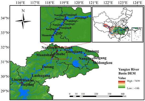
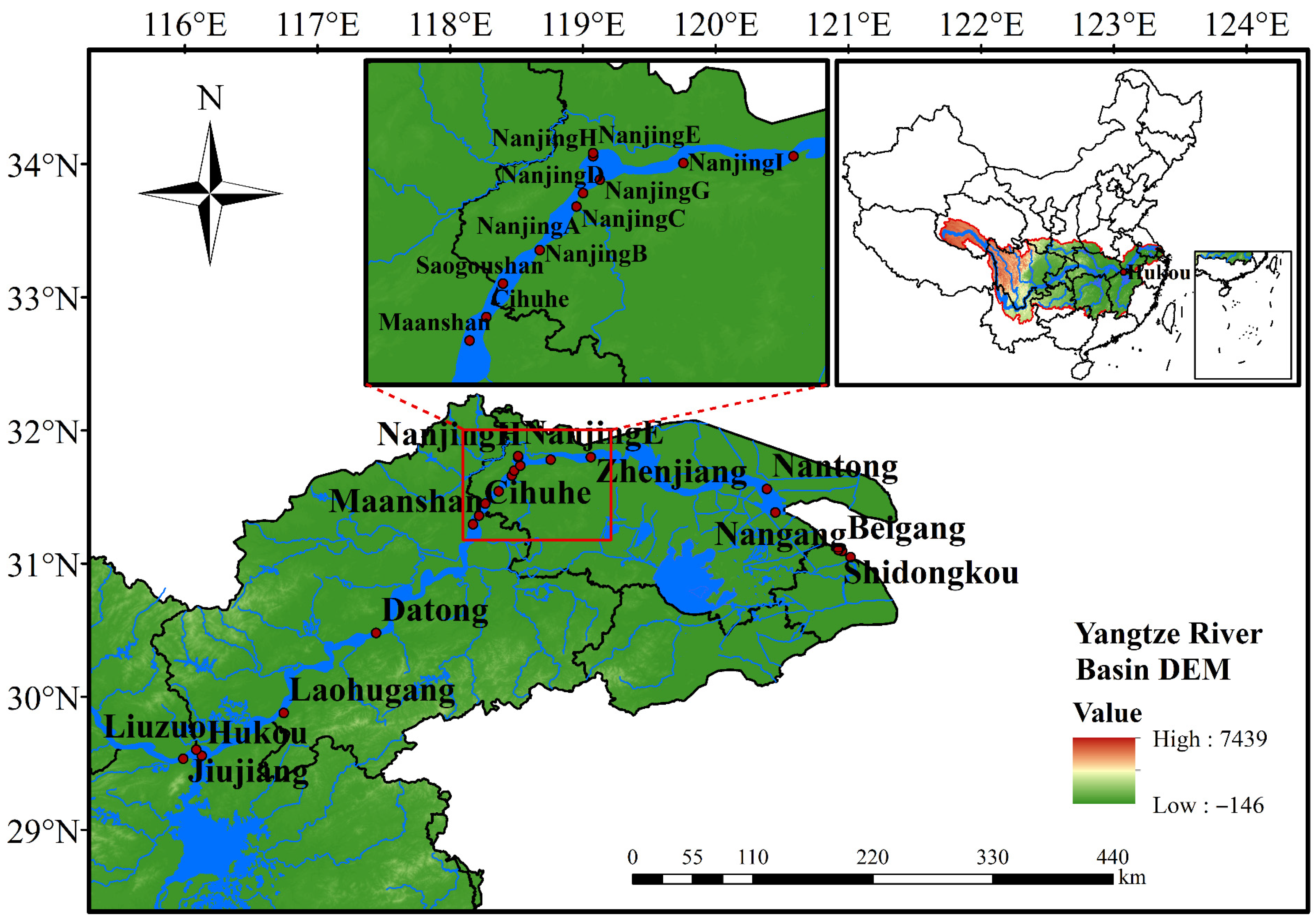
The lower reaches of the Yangtze River are about 938 km, with a catchment area of about 120,000 km², flowing through Jiangxi, Anhui, Jiangsu, Zhejiang, and Shanghai provinces, as shown in Figure 1. This watershed contains several national protected areas, such as the Poyang Lake Nature Reserve in Jiangxi Province, which is the world’s largest wintering habitat for whooping cranes and has important ecological value. Given the region’s ecological significance, the water temperature (WT) simulation is paramount.

Figure 1. Study area.

The primary tributaries of the lower reaches of the Yangtze River, such as the Qingyi River, Shuiyang River, and Huangpu River, are not large. This river segment is distinguished by the absence of a large-scale water conservancy project. The variation in the water level is small, with a depth of about 5~9 m [13], while the water surface width is about 2000 m [14]. Collectively, these hydromorphic properties, especially the wide water surface, require consideration of surface solar radiation (SSR) in WT simulation, as radiative heat exchange processes are important in such environments.

This study incorporates three hydro-meteorological parameters—air temperature (AT), SSR, and WT—derived from 22 stations distributed across the lower reaches of the Yangtze River, with measurements spanning the period 2008–2018. SSR is chosen among various heat flux components because it exhibits the strongest direct correlation with WT in this region. As shown in Table 1, the AT and SSR datasets are extracted from ECMWF Reanalysis v5 (ERA5), utilizing daily mean values at the 1000 hPa pressure level with a spatial resolution of 0.25° × 0.25°. The WT measurements come from monthly monitoring data obtained by the Changjiang Water Resources Commission of the Ministry of Water Resources of China.

Table 1. Data sources.

Data Type	Sources
Air temperature (AT)	ERA5 (https://cds.climate.copernicus.eu/datasets (accessed on 11 October 2024))
Surface solar radiation (SSR)	ERA5 (https://cds.climate.copernicus.eu/datasets (accessed on 11 October 2024))
Water temperature (WT)	Changjiang Water Resources Commission of the Ministry of Water Resources of China

2.2. Machine Learning Models

Three machine learning models were employed: a Back-Propagation Neural Network (BPNN), Random Forest (RF), and a Recurrent Neural Network (RNN). The BPNN and RF were selected as representative benchmarks (feedforward neural network and ensemble learning, respectively), while the RNN was chosen as the core model due to its ability to capture temporal dependencies inherent in water temperature series.

Each model has limitations: the BPNN is prone to overfitting and local optima; RF cannot model sequential structures without hand-crafted lag features; and the vanilla RNN suffers from vanishing/exploding gradients for long-term dependencies. The lag between AT/SSR and WT is only about one month (1–2 time steps), a length that is well within the capacity of a simple RNN.

More advanced recurrent architectures such as Long Short-Term Memory (LSTM) and Gated Recurrent Unit (GRU) are highly capable, especially when very long-term dependencies exist. With sufficiently long-term and detailed data, these models can achieve better simulation results for water temperature driven by AT and SSR. However, given the moderate length of our monthly data (2008–2018, about 132 time steps), LSTM or GRU would introduce many additional parameters and increase the risk of overfitting without providing meaningful performance gains in the current setting. Therefore, the simpler RNN is more appropriate for this study.

2.2.1. Back-Propagation Neural Network (BPNN)

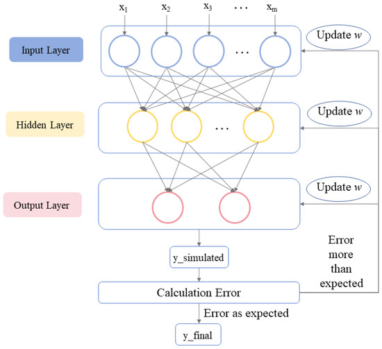
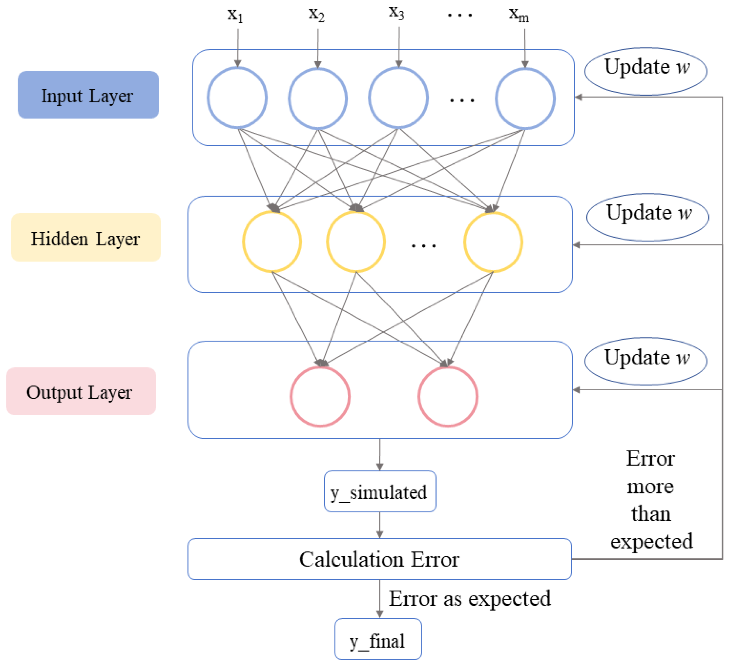
The Back-Propagation Neural Network (BPNN) is an artificial neural network trained using the error back-propagation algorithm. Its primary strengths lie in its robust self-learning capabilities and parallel computation. As shown in Figure 2, the BPNN architecture comprises three layers: the input layer, the hidden layer, and the output layer. The training process is bifurcated into two phases: forward propagation and backward propagation. During forward propagation, input data traverses sequentially through the network layers, generating outputs. Backward propagation involves calculating the error by comparing outputs with the actual values. Then, this error is retrogradely propagated, facilitating iterative adjustments to neuron weights and bias parameters to minimize simulation discrepancies.

Figure 2. Back-Propagation Neural Network flowchart.

The nodes of each layer are calculated as follows:

$$y=f\left({\displaystyle \sum w_i{x}_i+b}\right)$$

(1)

where x_i is the input data of the node, w is the weight of the node, b is the bias of the node, f is the activation function, and y is the output of the node.

2.2.2. Random Forest (RF)

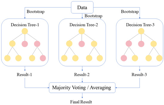
Random Forest (RF), a quintessential algorithm among bagging methods of ensemble learning, is distinguished by its high accuracy, user-friendly implementation, and inherent support for parallel processing. RF integrates multiple base models; i.e., multiple decision trees. Multiple decision trees with randomized samples and features are generated by bootstrapping, and then the final result is obtained by voting or averaging. The RF flowchart is shown in Figure 3.

Figure 3. Random Forest flowchart.

2.2.3. Recurrent Neural Network (RNN)

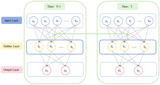
A Recurrent Neural Network (RNN) is a neural network that can process sequential data and remember historical information. Its strength lies in its capacity to process time-series information through cyclic connections that maintain an internal memory of historical states. As shown in Figure 4, the RNN framework comprises three layers: the input layer, which receives sequential data; the hidden layer, which contains recurrent units that propagate the temporal context; and the output layer, which generates simulations based on accumulated historical information. The output of the hidden layer is affected not only by the input at the current moment T, but also by the hidden layer at moment T − 1. The output layer obtains the final result based on the output of the hidden layer.

Figure 4. Recurrent Neural Network flowchart.

The S of the hidden layer is calculated as follows:

$$S_T=f\left(U\cdot X_T+W\cdot S_{T-1}\right)$$

(2)

The O of the output layer is calculated as follows:

$$O_T=g\left(V\cdot S_T\right)$$

(3)

where U is the weight from the input layer to the hidden layer, X_T is the input data at time T, W is the weight from the hidden layer at time T − 1 to the hidden layer at time T, S_T−1 is the value of the hidden layer at time T − 1, S_T is the value of the hidden layer at time T, f is the activation function, V is the weight from the hidden layer to the output layer, O_T is the value of the output layer, and g is a function.

2.3. Evaluation of Model Validity

To evaluate the simulation performance of the model, multiple indicators are selected: Nash–Sutcliffe Efficiency (NSE), Root Mean Square Error (RMSE), Mean Absolute Error (MAE), and Symmetric Mean Absolute Percentage Error (SMAPE).

NSE is commonly used to quantify the accuracy of simulation models (e.g., hydrological models) and takes values in the range (−∞, 1]. The closer the NSE is to 1, the better the model’s simulation ability. However, NSE has limitations: it is sensitive to extreme values and can be misleading when the observed data have low variance. Therefore, additional error metrics are necessary. The NSE formula is as follows:

$$NSE=1-{\displaystyle \frac{{\displaystyle \sum _{i=1}^n{\left(y_i-y_i^{simulated}\right)}^2}}{{\displaystyle \sum _{i=1}^n{\left(y_i-\stackrel{-}{y}\right)}^2}}}$$

(4)

RMSE is commonly used to measure the difference between the simulated and actual values; it takes values in the range [0, +∞). The smaller the RMSE, the smaller the model simulation error and the better the model. The formula is as follows:

$$RMSE=\sqrt{{\displaystyle \frac{1}{n}}{\displaystyle \sum _{i=1}^n{\left(y_i-y_i^{simulated}\right)}^2}}$$

(5)

MAE measures the average absolute difference between simulated and observed values; it takes values in the range [0, +∞). Compared to RMSE, MAE is less sensitive to outliers and provides a more robust error estimate. The formula is as follows:

$$MAE={\displaystyle \frac{1}{n}}{\displaystyle \sum _{i=1}^n\left|y_i-y_i^{simulated}\right|}$$

(6)

SMAPE, with a range of [0, 200%], is commonly used to measure the difference between the simulated and actual values when the data error is small. The smaller the SMAPE, the better. The formula is as follows [15]:

$$SMAPE={\displaystyle \frac{1}{n}}{\displaystyle \sum _{i=1}^n\frac{\left|y_i-y_i^{simulated}\right|}{\left(\left|y_i\right|+\left|y_i^{simulated}\right|\right)/2}}\times 100\%$$

(7)

where y_i^simulated is the simulated value, y_i is the actual value, $\stackrel{-}{y}$ is the mean of the actual values, and n is the number of data points.

2.4. Water Temperature Simulation Method Based on AT-SSR-RNN Coupling

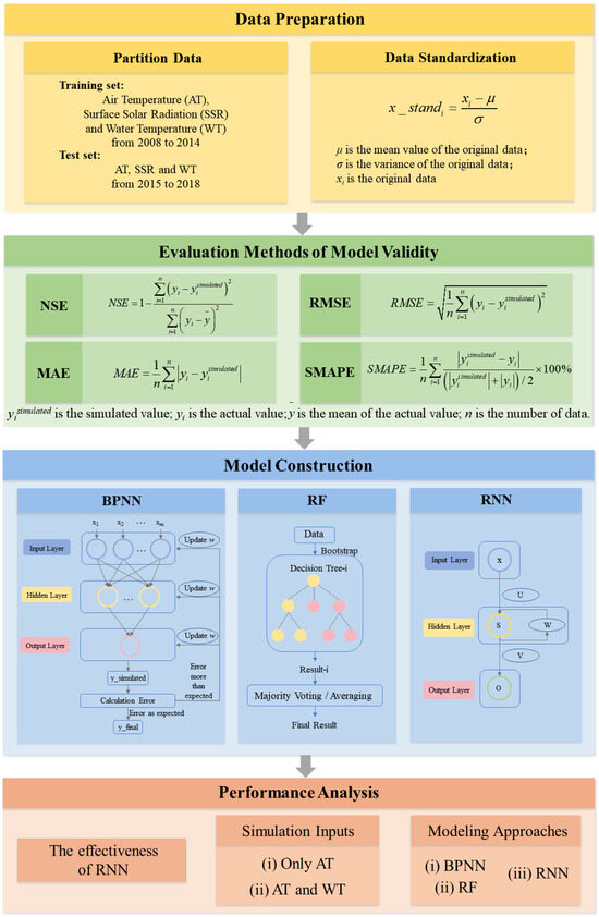
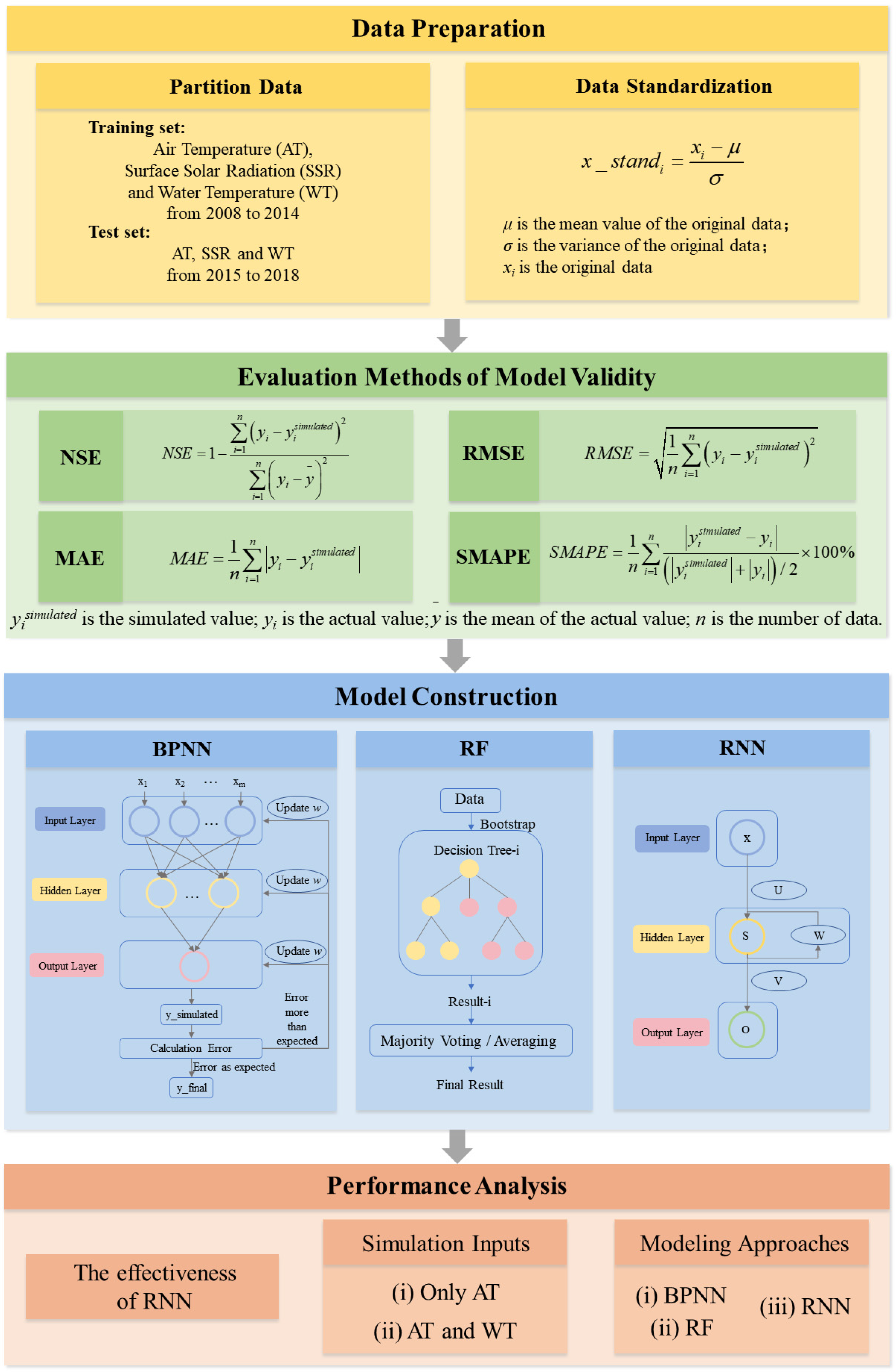
In this study, WT was simulated using AT and SSR data based on an RNN. The simulation flowchart is shown in Figure 5.

Figure 5. Flowchart of WT simulation based on AT-SSR-RNN coupling.

As shown in Figure 5, the WT simulation model is constructed from the collected data, and the results are analyzed through the following steps. (i) Data Preparation: AT, SSR, and WT data from 2008 to 2014 are used as the training set, and data from 2015 to 2018 are used as the test set. The data in the training and test sets are standardized. (ii) Evaluation Methods of Model Validity: The validity of the model is evaluated using four performance indicators: NSE, RMSE, MAE, and SMAPE. (iii) Model Construction: The model is trained using the standardized training dataset. The RNN architecture and training parameters are summarized in Table 2. Hyperparameter optimization is implemented via grid search with 5-fold cross-validation on the training set (2008–2014) to identify the optimal configuration. After obtaining the optimal parameters, the model is retrained on the full training set and evaluated on the independent test set (2015–2018). (iv) Performance Analysis: First, the effectiveness of the RNN model in WT simulation is evaluated by comparing simulated and actual WT. Second, improvements in model performance obtained by incorporating SSR as an additional input variable are quantitatively assessed relative to AT-only scenarios. Finally, the superiority of the RNN is demonstrated through comparative analysis against alternative modeling approaches.

Table 2. RNN model parameters.

Category	Specification
Hidden layers	1 SimpleRNN layer
Hidden layer activation	tanh
Number of RNN units	96
Output layer	1 Dense layer
Input sequence length	2 months
Loss function	Mean Squared Error (MSE)
Optimizer	Adam
Learning rate	0.0046
Batch size	36
Epochs	48

3. Results

3.1. AT and SSR Analysis of the Lower Reaches of the Yangtze River

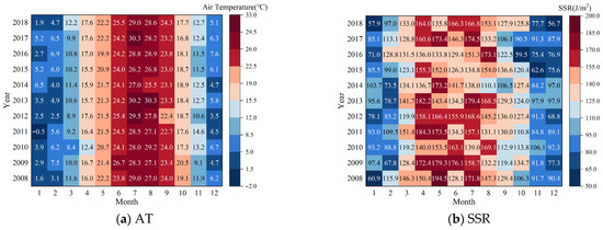
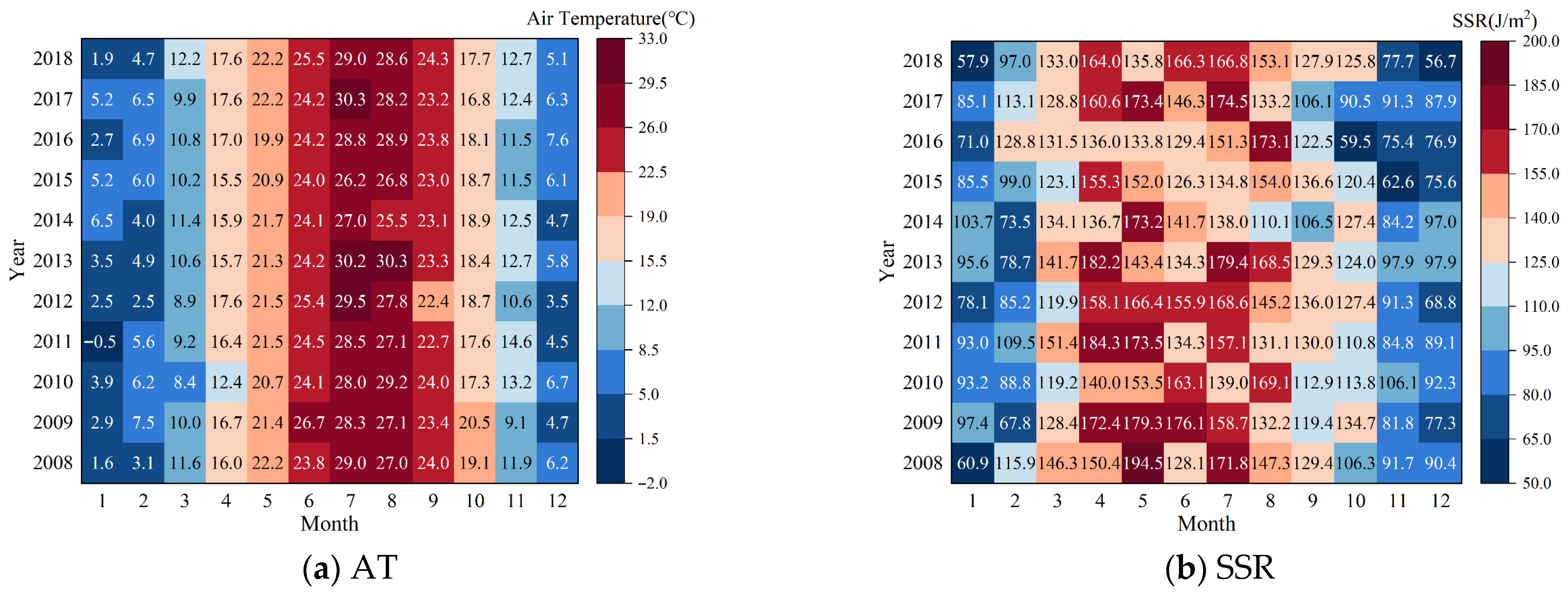
To characterize the variability in air temperature (AT) and surface solar radiation (SSR) in the lower reaches of the Yangtze River, monthly averages were computed. The results are shown in Figure 6.

Figure 6. Heat maps of AT and SSR from 2008 to 2018.

As shown in Figure 6a, analysis of the monthly AT distribution revealed a pronounced seasonal cycle. Commencing in March, AT progressively increased, reaching a peak exceeding 26.0 °C in July or August. Subsequently, AT markedly declined, reaching its annual nadir—typically below 5.0 °C—in January of the subsequent year. Notably, 2014 deviated from this pattern, with its minimum AT recorded in February rather than January. The mean annual AT across all study years was around 16.5 °C.

As shown in Figure 6b, the monthly SSR distribution followed a bimodal pattern with seasonal variability: an initial maximum occurring in April or May, followed by a secondary peak in July or August. After August, SSR progressively declined, reaching a minimum, typically below 80.0 J/m², in February of the subsequent year. Notably, SSR showed complex behavior between December and January in certain years. While it generally maintained its downward trend in December, occasional January rebounds were observed before the February nadir. The highest SSR exceeded 155.0 J/m² in each study year, with mean annual values of around 124.0 J/m².

The comparative analysis revealed a distinct temporal lag in AT relative to SSR. The annual SSR variation exhibited a bimodal distribution, with primary peaks occurring in April/May and secondary peaks in July/August, interspersed by a marked decline in June. This decline was particularly pronounced in certain years, such as 2008 and 2017. In contrast, AT followed a unimodal trajectory, featuring a gradual ascent followed by a descent. Notably, the AT maximum consistently lagged behind the secondary SSR peak by approximately one month. This phase-delay phenomenon is described in detail by Wu et al. [16].

3.2. WT Analysis of the Lower Reaches of the Yangtze River

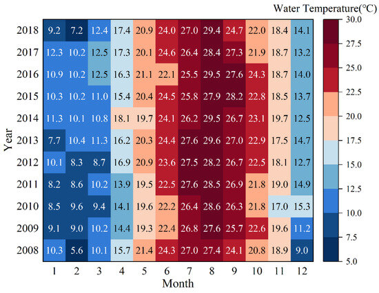
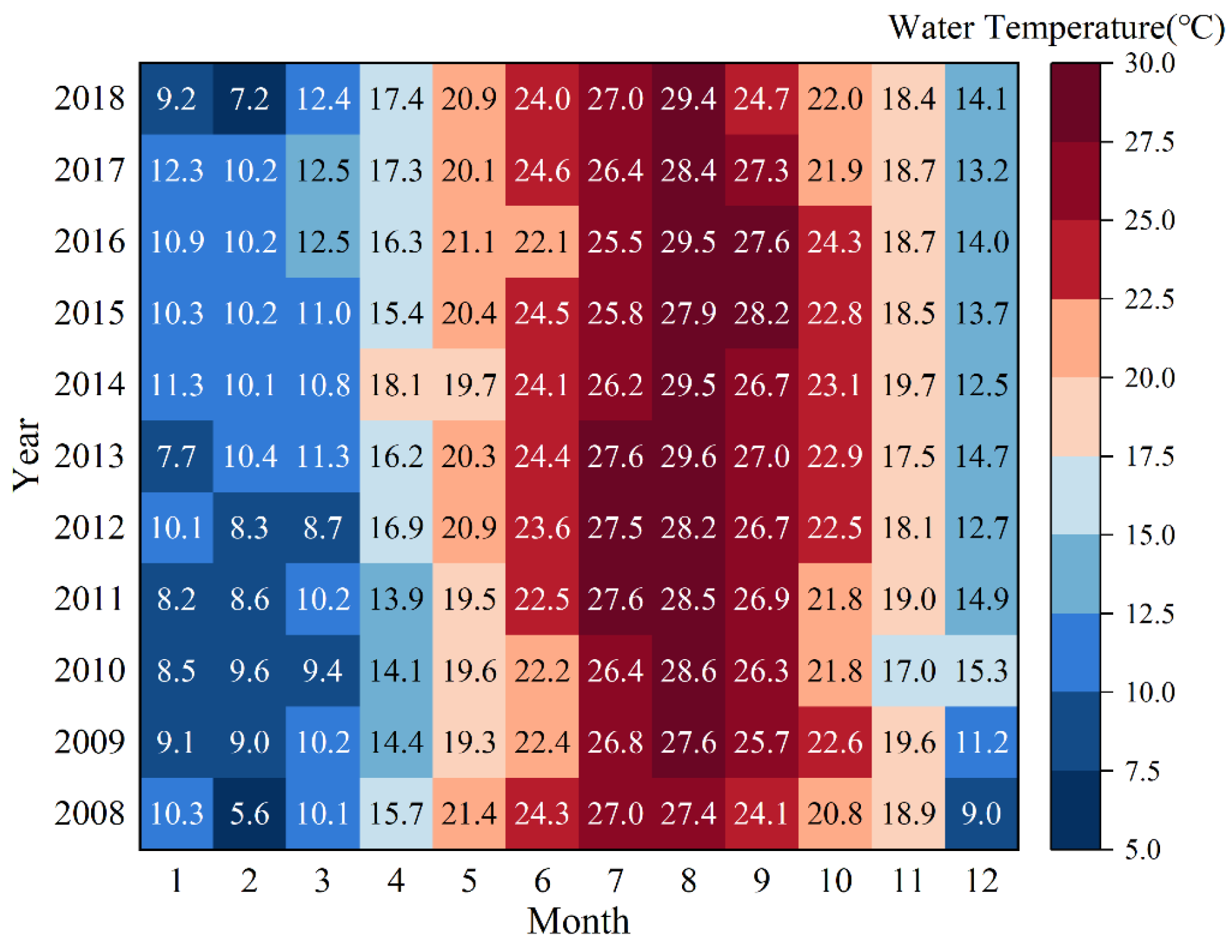
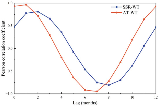
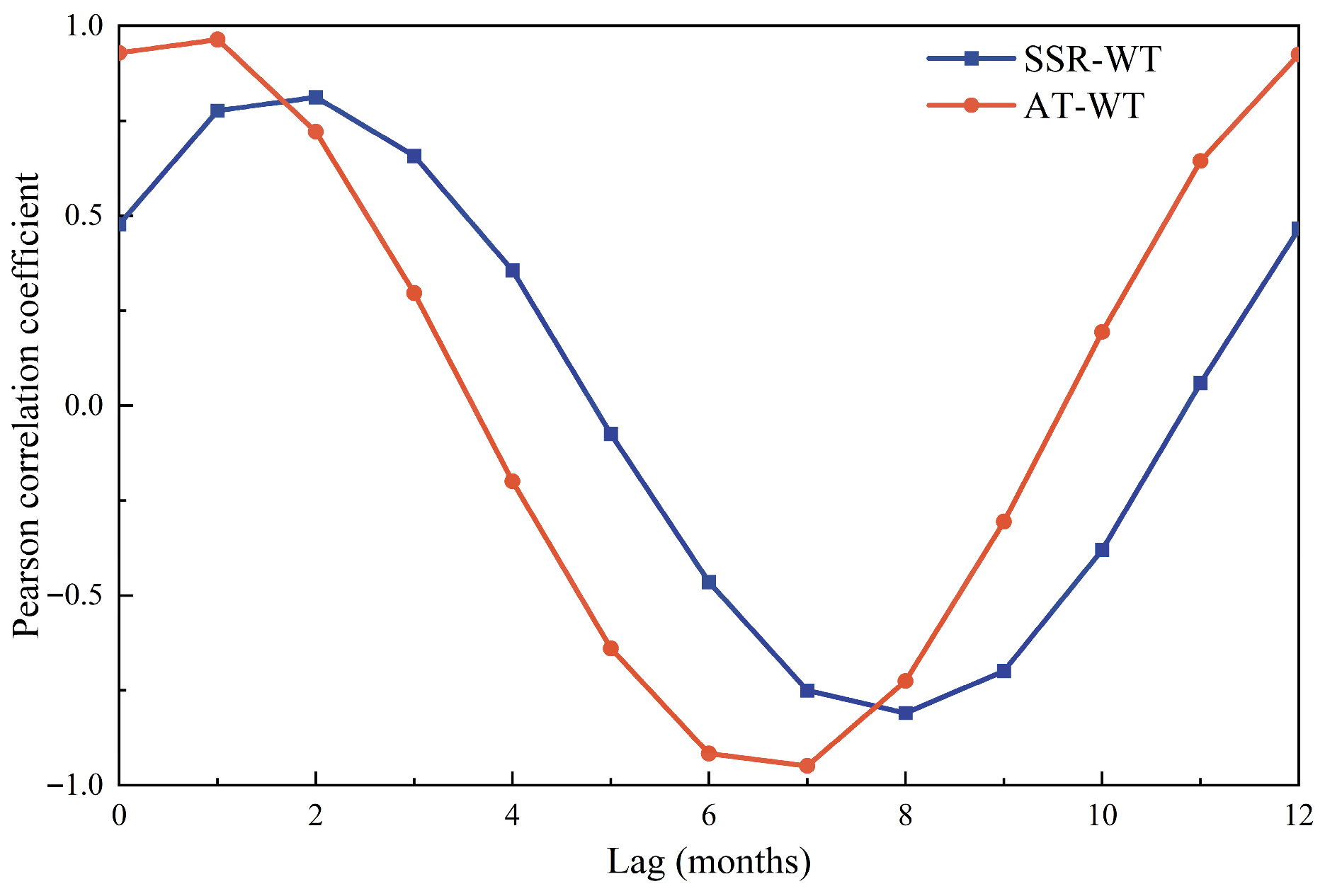
To investigate the variability in WT in the lower reaches of the Yangtze River, monthly mean water temperature (WT) values were computed. The results are shown in Figure 7 and Figure 8.

Figure 7. Heat map of WT from 2008 to 2018.

Figure 8. Lag correlation analysis.

As shown in Figure 7, the temporal evolution of WT reveals a distinct seasonal pattern. WT rises starting in March, peaks in August (>27.5 °C, except in 2015 when it peaked in September), and then declines to its minimum in January or February (<10.2 °C). The mean annual WT is approximately 18.8 °C.

WT lags behind AT and SSR. WT peaks in August, while AT peaks in July; the WT minimum occurs in February, about one month after the AT minimum (January). This lag is attributable to the higher heat capacity of water compared to that of air [17]. WT also lags behind SSR, with its annual maximum following the secondary SSR peak (in July) by approximately one month.

As shown in Figure 8, these lags were quantified through cross-correlation analysis of the monthly time series (2008–2018). The maximum correlation between AT and WT is 0.9644 at a lag of +1 month, confirming that WT lags AT by one month. For SSR and WT, the peak correlation is 0.8125 at a lag of +2 months, indicating that WT is slower to respond to solar radiation due to the bimodal annual SSR distribution and the cumulative heating effect.

3.3. Results of WT Simulation Based on AT-SSR-RNN Coupling

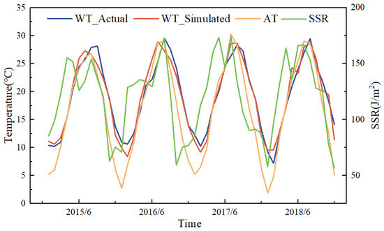
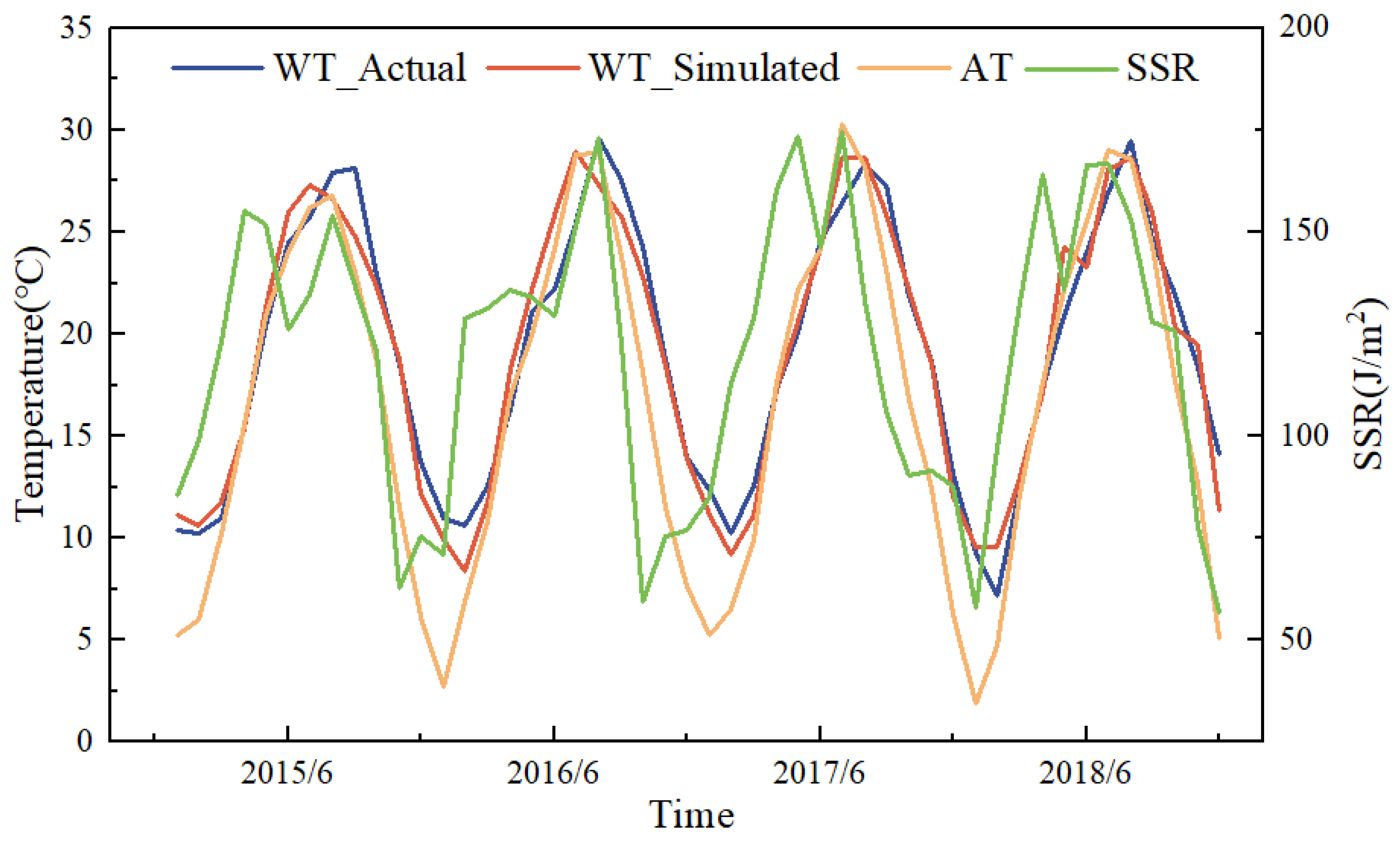
To evaluate the performance of the AT-SSR-RNN coupling model in simulating WT, the monthly averages of four variables were analyzed: AT, SSR, actual WT, and simulated WT. The results are shown in Figure 9 and Table 3.

Figure 9. Results for the test period.

Table 3. Extreme values in the test period and their times of occurrence.

Year		WT_Actual (°C)	WT_Simulated (°C)	AT (°C)	SSR (J/m2)
2015	Max	28.13 (September)	27.28 (July)	26.80 (August)	155.30 (April)
	Min	10.22 (February)	10.59 (February)	5.20 (January)	62.60 (November)
2016	Max	29.59 (August)	28.93 (July)	28.90 (August)	173.10 (August)
	Min	10.61 (February)	8.35 (February)	2.70 (January)	59.50 (October)
2017	Max	28.38 (August)	28.66 (August)	30.30 (July)	174.50 (July)
	Min	10.27 (February)	9.17 (February)	5.20 (January)	85.10 (February)
2018	Max	29.44 (August)	28.68 (August)	29.00 (July)	166.80 (July)
	Min	7.20 (February)	9.56 (January)	1.90 (January)	56.70 (December)

As shown in Figure 9, the AT-SSR-RNN model simulates WT in the lower Yangtze River reasonably well, with simulated values generally following observed fluctuations. However, certain systematic deviations exist. First, the model produces a narrower temperature range: observed WT spans 7.20–29.59 °C, while simulated WT spans 8.35 –28.93 °C. Second, during 2015–2016, the simulated maximum WT occurs one month earlier than the observed peak; the simulated minimum in 2018 also appears one month early.

A narrower simulated temperature range suggests that the model tends to produce values closer to the mean, a common behavior in data-driven models when extreme events are underrepresented in the training set [18]. The early simulated peaks in 2015–2016 imply that the model responds to atmospheric forcing more quickly than the real water body. In contrast, observed WT changes are delayed by the high thermal inertia of water and by vertical mixing (wind-induced and convective), which redistributes surface heat input and buffers rapid temperature variations. The vanilla RNN architecture also has a limited ability to distinguish subtle temporal dependencies under irregular forcing [19].

Compared to AT, simulated WT generally follows the same trend but differs at extremes; for example, in 2015–2016, the simulated peak occurs in July, one month ahead of the August AT peak. The simulated WT also deviates from the typical one-month lag behind SSR, with the model placing the July peak two months earlier than the observed August peak. These mismatches indicate that the current statistical model does not fully reproduce the thermal inertia of the water body, suggesting that incorporating additional physical constraints could improve future simulations.

4. Discussion

4.1. The Validity of WT Simulation Based on AT-SSR-RNN Coupling

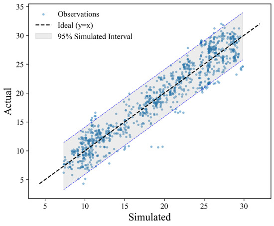
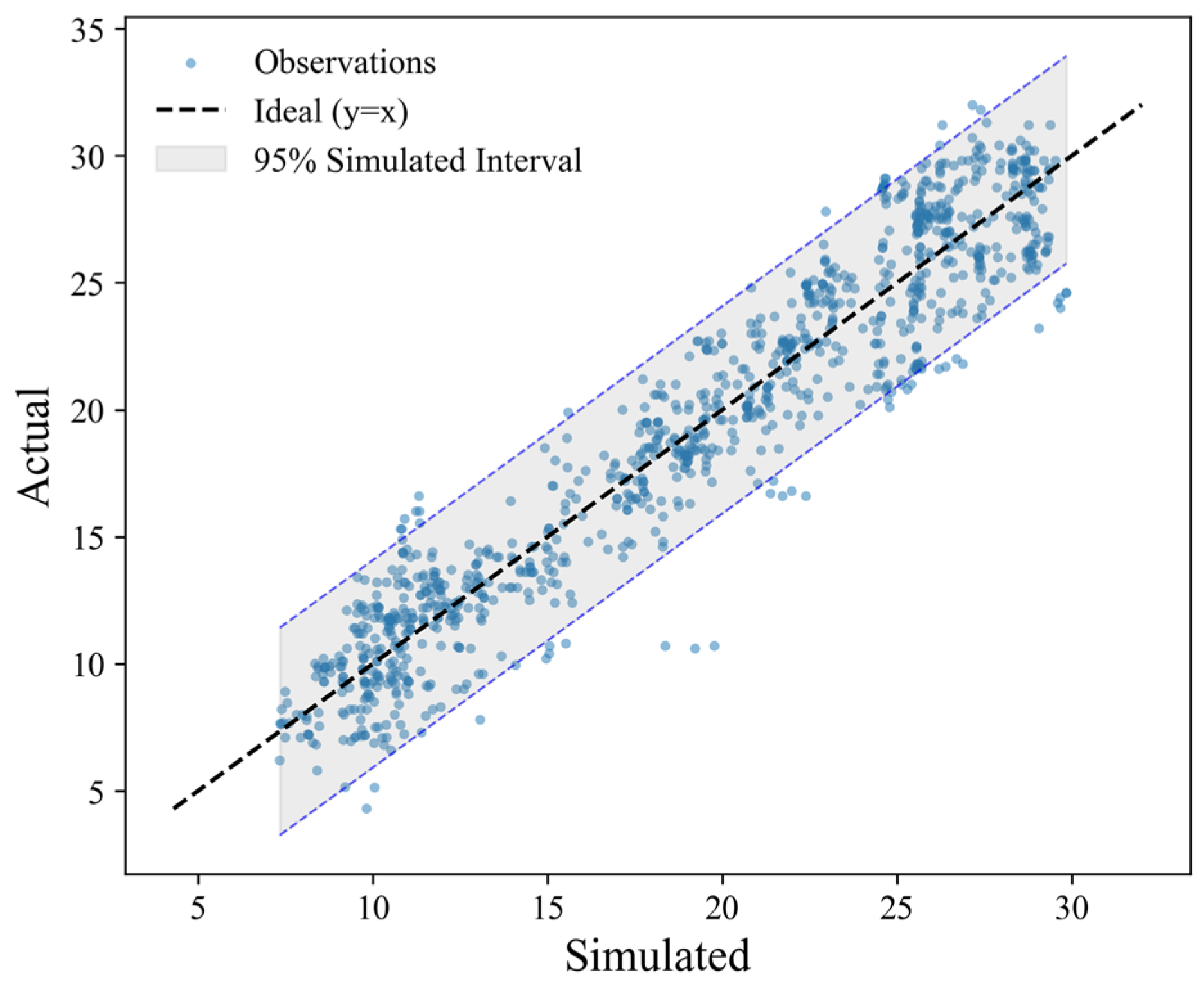
The residuals and evaluation indicators of the constructed model on the test set were calculated, with the 95% confidence intervals plotted accordingly. The results of these calculations are compared and presented in Figure 10 and Table 4 and Table 5.

Figure 10. Confidence interval for WT simulation (test).

Table 4. The results for the residuals (test).

Statistic	Value
Mean of residuals (°C)	−0.0106
Standard deviation of residuals (°C)	2.08
95% CI for mean of residuals (°C)	[−0.1362, 0.1150]

Table 5. Evaluation indicator results.

Dataset	NSE	RMSE (°C)	MAE (°C)	SMAPE
Training set	0.9260	2.00	1.54	10.18%
Test set	0.9100	2.08	1.65	9.61%

As demonstrated in Figure 10 and Table 4, the model shows no significant systematic bias. Residual analysis on the test set yields a mean residual (observed minus simulated) of −0.0106 °C, very close to zero, with a standard deviation of 2.08 °C. The 95% confidence interval for the mean residual is [−0.1362 °C, 0.1150 °C], which includes zero. Based on the residual standard deviation, the approximate 95% prediction interval for a new observation is ±4.08 °C. These results demonstrate that the model produces unbiased estimates with quantified uncertainty.

As shown in Table 5, the AT-SSR-RNN model exhibits strong performance in simulating water temperature. On the training set, NSE = 0.9260, RMSE = 2.00 °C, MAE = 1.54 °C, and SMAPE = 10.18%. On the test set, NSE = 0.9100, RMSE = 2.08 °C, MAE = 1.65 °C, and SMAPE = 9.61%. These metrics indicate a very good model, according to Chicco et al. [15]. The high NSE values further confirm the model’s reliability [20]. The lower SMAPE on the test set (9.61% vs. 10.18%) suggests a slight overestimation, as SMAPE penalizes underestimation more heavily [21,22,23].

4.2. The Advantages of Considering SSR in WT Simulation

Two WT simulation models were constructed based on the RNN: one that solely considers AT and one that comprehensively integrates both AT and SSR. The results of these WT simulations were subsequently compared against actual values, with the results presented in Table 6.

Table 6. Evaluation indicator results with and without consideration of SSR.

Inputs (Test Set)	NSE	RMSE (°C)	MAE (°C)	SMAPE
AT	0.8411	2.76	2.37	14.37%
AT and SSR	0.9100	2.08	1.65	9.61%

As shown in Table 6, the model that takes into account both SSR and AT exhibits superior performance to the model that considers only AT. NSE increases by 8.2%, RMSE drops by 24.6%, MAE decreases by 30.4%, and SMAPE falls by 33.1%.

The improved performance can be explained by the physical role of SSR in the lower Yangtze River (width ~2000 m, depth 5–9 m). Solar radiation first warms the surface layer; turbulent mixing (wind-induced and convective) then redistributes heat downward, delaying the bulk water temperature response. In contrast, AT affects the surface through sensible and latent heat exchange, producing a shorter lag of one month. A purely AT-driven model cannot fully represent this cumulative radiative heating effect.

The importance of SSR as a primary heat flux driver has been widely recognized. Benyahya et al. identified SSR as the key determinant of heat flux in streams [24]. Yang et al. found that among Arctic rivers, the river with the highest heat flux also had the warmest water temperature [25]. Studies on lakes [26] and streams [27] further confirm that solar radiation is a major factor driving surface water temperature. Similar physical controls have been reported in large river systems [28]. These findings support the inclusion of SSR as an explicit input in water temperature modeling.

4.3. The Advantages of the RNN over Traditional Methods

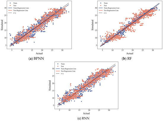
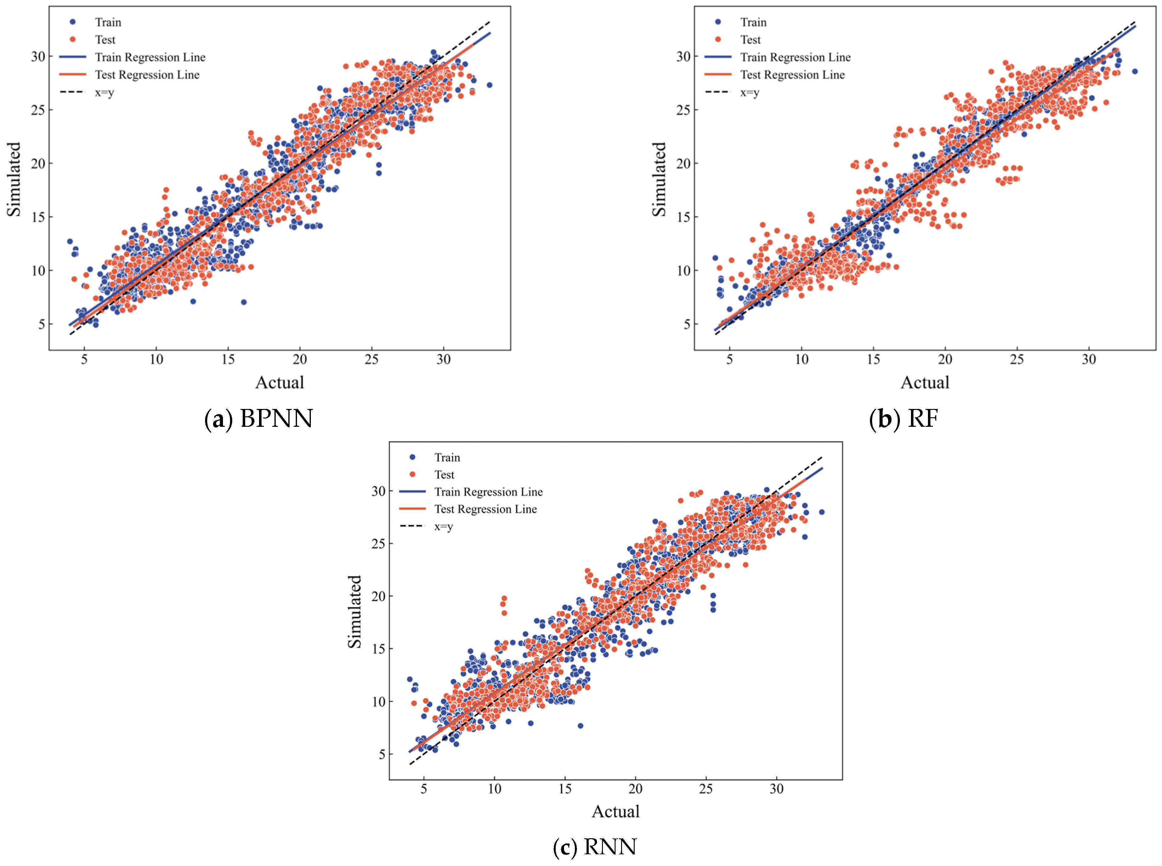
In this study, three algorithms—Back-Propagation Neural Network (BPNN), Random Forest (RF), and Recurrent Neural Network (RNN)—were employed to simulate WT based on AT and SSR. The simulated and actual values are compared in Figure 11 and Table 7.

Figure 11. WT simulation results of different models considering AT and SSR.

Table 7. Comparison of simulation effects of different models.

Model	NSE	RMSE (°C)	MAE (°C)	SMAPE
RNN	0.9100	2.08	1.65	9.61%
BP	0.9030	2.16	1.70	10.23%
RF	0.8751	2.45	1.92	11.95%

The RNN model’s simulation performance is superior to that of the BPNN and RF. As shown in Figure 11, the regression line corresponding to the RNN model aligns most closely with the x = y line, suggesting that the simulated values generated by the RNN model are the closest to the actual values. On the test set, the RNN model achieves the highest NSE (0.9100) and the lowest RMSE (2.08 °C), MAE (1.65 °C), and SMAPE (9.61%), followed by the BPNN (NSE: 0.9030, RMSE: 2.16 °C, MAE: 1.70 °C, SMAPE: 10.23%) and RF (NSE: 0.8751, RMSE: 2.45 °C, MAE: 1.92 °C, SMAPE: 11.95%).

The inferior performance of RF and the BPNN can be explained by their structural limitations. RF’s worst performance can potentially be attributed to overfitting [29], as it achieved the highest NSE on the training set (0.9839), but it dropped sharply on the test set. The BPNN model does not perform as well as the RNN model, likely due to its inability to directly model time dependencies. In contrast, the RNN model is adept at capturing long-term dependencies when processing sequential data [30], a characteristic that makes it a frequent choice for time-series simulations [31,32].

As shown in Table 7, the RNN’s improvement over the BPNN appears modest (RMSE reduction: 0.08 °C, 3.7%), but the difference carries practical ecological significance. Feigl et al. reported that the median difference in Root Mean Square Error (RMSE) among six machine learning models used for river temperature forecasting was only 0.08 °C and noted that Recurrent Neural Networks (RNNs) performed best when long-term dependencies were present [33], consistent with the findings of this study. Furthermore, WT is an ecological “master factor” in controlling aquatic organism growth and survival. Small changes in water temperature can have large effects on salmonid growth and survival [34]. Similarly, the early growth stages of Coreius guichenoti, an endemic fish in the Yangtze River, are highly sensitive to WT fluctuations [35].

5. Conclusions

The Recurrent Neural Network (RNN) model based on the coupling of air temperature (AT) and surface solar radiation (SSR) achieves highly applicable simulation results. Specifically, the model achieved a Nash–Sutcliffe Efficiency (NSE) exceeding 0.900, Root Mean Square Error (RMSE) of 2.08 °C, Mean Absolute Error (MAE) of 1.65 °C, and Symmetric Mean Absolute Percentage Error (SMAPE) of merely 9.61%. Residual analysis confirmed no significant systematic bias (mean residual = −0.0106 °C), and the 95% prediction interval for a new observation was approximately ±4.08 °C. The simulated WT trends align with the actual WT data, with only slight deviations noted at the extreme points.

The WT trend lags slightly behind those of AT and SSR and is flatter. AT starts to rise in March, peaks above 26 °C in July or August, and then declines to a minimum below 5 °C in January. SSR begins to increase in March, reaching a first high in April or May and a second high in July or August (>155.0 J/m²), and then decreases to a minimum below 80 J/m² in February. WT typically peaks in August (>27.5 °C) and reaches its minimum in January or February (<10.2 °C). Cross-correlation analysis confirmed that WT lags AT by one month and SSR by two months.

The results demonstrate the importance of considering SSR as a simulation input. Compared to the AT-only model, the AT-SSR-RNN model improved NSE by 8.2% (from 0.8411 to 0.9100), reduced RMSE by 24.6% (from 2.76 °C to 2.08 °C), lowered MAE by 30.4% (from 2.37 °C to 1.65 °C), and decreased SMAPE by 33.1% (from 14.37% to 9.61%). These improvements show that the performance of the model is improved when SSR is considered.

Among the modeling approaches, the RNN demonstrated superior performance in capturing temporal dependencies within the dataset. The RNN achieved the highest NSE value of 0.9100, followed by the BPNN (0.9030) and RF (0.8751). Consistent with this pattern, the RNN achieved the lowest simulation errors (RMSE: 2.08 °C, SMAPE: 9.61%), outperforming both the BPNN (RMSE: 2.16 °C, SMAPE: 10.23%) and Random Forest (RF) models (RMSE: 2.45 °C, SMAPE: 11.95%). These results collectively underscore that the proposed AT-SSR-RNN coupling method is most suitable for simulating WT in this study.

References

- Lu, Q.; Duckett, F.; Nairn, R.; Brunton, A. 3-D eutrophication modeling for Lake Simcoe, Canada. In Proceedings of the AGU Fall Meeting Abstracts, the AGU Fall Meeting, San Francisco, CA, USA, 11–15 December 2006. Abstract H23B-1496. [Google Scholar]
- Lee, H.; Chung, S.; Ryu, I.; Choi, J. Three-dimensional modeling of thermal stratification of a deep and dendritic reservoir using ELCOM model. J. Hydro-Environ. Res. 2013, 7, 124–133. [Google Scholar] [CrossRef] [Scilit]
- Arifin, R.R.; James, S.C.; de Alwis Pitts, D.A.; Hamlet, A.F.; Sharma, A.; Fernando, H.J. Simulating the thermal behavior in Lake Ontario using EFDC. J. Great Lakes Res. 2016, 42, 511–523. [Google Scholar] [CrossRef] [Scilit]
- Johnson, F.A. Stream temperatures in an alpine area. J. Hydrol. 1971, 14, 322–336. [Google Scholar] [CrossRef] [Scilit]
- Smith, K. The prediction of river water temperatures/prédiction des températures des eaux de rivière. Hydrol. Sci. J. 1981, 26, 19–32. [Google Scholar] [CrossRef] [Scilit]
- Cheng, T.; Wang, J.; Sui, J.; Song, F.; Fu, H.; Wang, T.; Guo, X. Simulation and prediction of water temperature in a water transfer channel during winter periods using a new approach based on the wavelet noise reduction-deep learning method. J. Hydrol. Hydromech. 2024, 72, 49–63. [Google Scholar] [CrossRef] [Scilit]
- Yang, K.; Guo, X.; Wang, T.; Fu, H.; Pan, J. Effects of solar radiation and ground temperature on water temperature under ice cover. J. Hydraul. Eng. 2022, 53, 530–538. [Google Scholar]
- Suaza-Sierra, I.; Moreno, H.A.; De la Fuente, L.A.; Neeson, T.M. Interpretable machine learning for reservoir water temperatures in the US Red River Basin of the South. arXiv 2025, arXiv:2511.01837. [Google Scholar] [CrossRef] [Scilit]
- Li, Z.; Zhang, Z.; Xiong, S.; Zhang, W.; Li, R. Lake surface temperature predictions under different climate scenarios with machine learning methods: A case study of Qinghai lake and Hulun lake, China. Remote Sens. 2024, 16, 3220. [Google Scholar] [CrossRef] [Scilit]
- Wang, C.; Dong, S.; Bouazza, A.; Ding, X. Explainable machine learning models to predict outlet water temperature of pipe-type energy pile. Renew. Energy 2025, 246, 122972. [Google Scholar] [CrossRef] [Scilit]
- Sehovac, L.; Grolinger, K. Deep learning for load forecasting: Sequence to sequence recurrent neural networks with attention. IEEE Access 2020, 8, 36411–36426. [Google Scholar] [CrossRef] [Scilit]
- Mienye, I.D.; Swart, T.G.; Obaido, G. Recurrent neural networks: A comprehensive review of architectures, variants, and applications. Information 2024, 15, 517. [Google Scholar] [CrossRef] [Scilit]
- Li, X.; Zhou, Z.Y.; Zuo, L.Q.; Sun, M.; Wang, H.Y.; Huang, T.J. Study on the maximum stable navigation depth of the bifurcated reach from Hukou to Nanjing in the lower reaches of the Yangtze River. Port. Waterw. Eng. 2022, 11, 116–121. [Google Scholar]
- Yang, J.; Huang, X.; Tang, Q. Satellite-derived river width and its spatiotemporal patterns in China during 1990–2015. Remote Sens. Environ. 2020, 247, 111918. [Google Scholar] [CrossRef] [Scilit]
- Chicco, D.; Warrens, M.J.; Jurman, G. The coefficient of determination R-squared is more informative than SMAPE, MAE, MAPE, MSE and RMSE in regression analysis evaluation. PeerJ Comput. Sci. 2021, 7, e623. [Google Scholar] [CrossRef] [Scilit]
- Wu, G.; Zhang, C.; Zhao, R.; Qin, P.; Qin, Y. Asymmetries of the lag between air temperature and insolation in gauge observations and reanalyses over China. Atmos. Res. 2023, 288, 106729. [Google Scholar] [CrossRef] [Scilit]
- Feng, J.W.; Liu, H.Z.; Sun, J.H.; Wang, L. The surface energy budget and interannual variation of the annual total evaporation over a highland lake in Southwest China. Theor. Appl. Climatol. 2016, 126, 303–312. [Google Scholar] [CrossRef] [Scilit]
- Corona, C.R.; Hogue, T.S. Machine Learning in Stream/River Water Temperature Modelling: A review and metrics for evaluation. Hydrol. Earth Syst. Sci. Discuss. 2024, 2024, 1–38. [Google Scholar]
- Waqas, M.; Humphries, U.W. A critical review of RNN and LSTM variants in hydrological time series predictions. MethodsX 2024, 13, 102946. [Google Scholar] [CrossRef] [Scilit] [PubMed]
- Legates, D.R.; McCabe, G.J., Jr. Evaluating the use of “goodness-of-fit” measures in hydrologic and hydroclimatic model validation. Water Resour. Res. 1999, 35, 233–241. [Google Scholar] [CrossRef] [Scilit]
- Chen, C.; Twycross, J.; Garibaldi, J.M. A new accuracy measure based on bounded relative error for time series forecasting. PLoS ONE 2017, 12, e0174202. [Google Scholar] [CrossRef] [Scilit]
- Makridakis, S.; Spiliotis, E.; Assimakopoulos, V. The M4 Competition: Results, findings, conclusion and way forward. Int. J. Forecast. 2018, 34, 802–808. [Google Scholar] [CrossRef] [Scilit]
- Bandara, K.; Bergmeir, C.; Smyl, S. Forecasting across time series databases using recurrent neural networks on groups of similar series: A clustering approach. Expert. Syst. Appl. 2020, 140, 112896. [Google Scholar] [CrossRef] [Scilit]
- Benyahya, L.; Caissie, D.; Satish, M.G.; El-Jabi, N. Long-wave radiation and heat flux estimates within a small tributary in Catamaran Brook (New Brunswick, Canada). Hydrol. Process. 2012, 26, 475–484. [Google Scholar] [CrossRef] [Scilit]
- Yang, D.; Shrestha, R.R.; Lung, J.L.Y.; Tank, S.; Park, H. Heat flux, water temperature and discharge from 15 northern Canadian rivers draining to Arctic Ocean and Hudson Bay. Global Planet. Change 2021, 204, 103577. [Google Scholar] [CrossRef] [Scilit]
- Shinohara, R.; Tanaka, Y.; Kanno, A.; Matsushige, K. Relative impacts of increases of solar radiation and air temperature on the temperature of surface water in a shallow, eutrophic lake. Hydrol. Res. 2021, 52, 916–926. [Google Scholar] [CrossRef] [Scilit]
- Maheu, A.; Caissie, D. Spatial and temporal variability of the solar radiation heat flux in streams of a forested catchment. Can. Water Resour. J. 2023, 48, 206–221. [Google Scholar] [CrossRef] [Scilit]
- Bray, E.N.; Modar, N.; Dozier, J. Atmospheric controls on river temperature: Sensitivity of river temperature downstream of a dam to changes in a Mediterranean climate. J. Hydrol. Reg. Stud. 2025, 60, 102500. [Google Scholar] [CrossRef] [Scilit]
- Murphy, K.P. Probabilistic Machine Learning: An Introduction; MIT Press: Cambridge, MA, USA, 2022. [Google Scholar]
- Feng, J.; Yang, L.T.; Ren, B.; Zou, D.; Dong, M.; Zhang, S. Tensor recurrent neural network with differential privacy. IEEE Trans. Comput. 2023, 73, 683–693. [Google Scholar] [CrossRef] [Scilit]
- Xia, M.; Shao, H.; Ma, X.; De Silva, C.W. A stacked GRU-RNN-based approach for predicting renewable energy and electricity load for smart grid operation. IEEE Trans. Ind. Inform. 2021, 17, 7050–7059. [Google Scholar] [CrossRef] [Scilit]
- Zaheer, S.; Anjum, N.; Hussain, S.; Algarni, A.D.; Iqbal, J.; Bourouis, S.; Ullah, S.S. A multi parameter forecasting for stock time series data using LSTM and deep learning model. Mathematics 2023, 11, 590. [Google Scholar] [CrossRef] [Scilit]
- Feigl, M.; Lebiedzinski, K.; Herrnegger, M.; Schulz, K. Machine-learning methods for stream water temperature prediction. Hydrol. Earth Syst. Sci. 2021, 25, 2951–2977. [Google Scholar] [CrossRef] [Scilit]
- Brewitt, K.S.; Danner, E.M. Spatio-temporal temperature variation influences juvenile steelhead (Oncorhynchus mykiss) use of thermal refuges. Ecosphere 2014, 5, 1–26. [Google Scholar] [CrossRef] [Scilit]
- Li, X.; Wu, X.; Li, X.; Zhu, T.; Zhu, Y.; Chen, Y.; Wu, X.; Yang, D. Effects of water temperature on growth performance, digestive enzymes activities, and serum indices of juvenile Coreius guichenoti. J. Therm. Biol. 2023, 115, 103595. [Google Scholar] [CrossRef] [Scilit]
Disclaimer/Publisher’s Note: The statements, opinions and data contained in all publications are solely those of the individual author(s) and contributor(s) and not of MDPI and/or the editor(s). MDPI and/or the editor(s) disclaim responsibility for any injury to people or property resulting from any ideas, methods, instructions or products referred to in the content. |
© 2026 by the authors. Licensee MDPI, Basel, Switzerland. This article is an open access article distributed under the terms and conditions of the Creative Commons Attribution (CC BY) license.