


Abstract
In the domain of river engineering, estimating the total sediment load in rivers is a crucial challenge. For tens to hundreds of kilometers downstream, the additional sand and gravel in the sediment can raise the elevation of channel beds. For highly braided rivers like the Brahmaputra-Jamuna, the accurate prediction of the total sediment load depends on the complex relationships among different hydro-meteorological variables. As a result, manual selection of the lagged features from only antecedent sediment records can produce suboptimal predictions, which can be considered a significant research gap. In addition, the predictive accuracy can be further enhanced through the application of advanced decomposition techniques. To address these deficiencies, we implemented three sophisticated feature selection methodologies: SelectKBest, Mutual Information, and Random Forest utilizing the Boruta Algorithm as an alternative to manual feature selection. Furthermore, we investigated complete ensemble empirical mode decomposition with adaptive noise (CEEMDAN), variational mode decomposition (VMD), and the Hodrick–Prescott Filter (HPF) to improve data mining efficiency. Four distinct artificial neural network (ANN) training algorithms were considered: back propagation (BP), cascade correlation (CC), conjugate gradient (CG), and Levenberg–Marquardt (LM), as alternatives to the conventional BP-based training approach. The effectiveness of the variants of the ANN was assessed in comparison to a powerful ensemble learning model, specifically the decision tree (DT). Results indicate that the HPF-enhanced ANN-LM model exhibited the strongest performance metrics when compared to alternative techniques, with values of NRMSE = 0.004, MAE = 455.242 kg/s, NSE = 0.998, and KGE = 0.990. The outcomes from Sobol’s sensitivity analysis suggest that the sediment dynamics in this region can be better predicted through the inclusion of rainfall-based features.
1. Introduction
The Brahmaputra-Jamuna is classified as a sand-bed river, exhibiting a median bed-material size () that ranges from 0.22 mm in the upstream portion to 0.16 mm in the downstream part [1]. Coleman (1969) [2] reported that the sediment load of the Brahmaputra-Jamuna was 555 Mt y−1 in the beginning of the 1960s. River sediment has the ability to raise channel beds with an accumulation of gravel and sand, propagating this effect for several kilometers downstream. This aggradation facilitates the lateral movement of channels, eventually resulting in significant flooding during extreme rainfall events, as it reduces the capacity of the channel required to transport the excessive flow during flooding [3]. Therefore, accurate prediction of sediment transport levels in alluvial rivers, such as the Brahmaputra-Jamuna River system, is crucial for understanding the localized pattern of sedimentation, erosion, flood control, and long-term morphological analysis.
Over the past several decades, comprehensive research has resulted in an extensive variety of sediment transport models. Li and Yang (2022) [4] utilized three predictive models: support vector machine (SVM), ensemble learning (EL), and long short-term memory (LSTM). They incorporated seasonal adjustment (SA) and Bayesian optimization to model the suspended sediment load (SSL). The analysis was constructed exclusively on the lagged features obtained from the antecedent SSL records. Huang et al. (2021) [5] designed their input structure through the incorporation of suspended sediment concentration (SSC) records from nearby measuring stations, which worked well in their study but can be found difficult in data-scarce regions.
Hanoon et al. (2022) [6] conducted a comparative analysis of multiple machine learning (ML) models, including gradient boost regression (GBT), support vector machine (SVM), random forest (RF), and artificial neural network (ANN), for predicting SSL at the Rantau Panjang station on the Johor River basin (JRB), Malaysia, utilizing lag features derived from historical SSL and discharge records. A comparable input structure was chosen by Band et al. (2026) [7] for SSL prediction of the Mississippi River in the United States, where they explored RF, LSTM, and recurrent neural networks (RNN), along with their hybrid RNN-LSTM optimized by the Immune System Algorithm (ISA).
Gharehbaghi et al. (2026) [8] predicted the SSL of the Mississippi River in the United States through RNN, BiRNN, hybrid RNN-CNN, hybrid BiRNN-CNN, adaptive boosting (AdaBoost), natural gradient boosting (NGBoost), and GBT. This study also applied the antecedent discharge and SSL values as their model input. Kumar et al. (2025) [9] employed three input variables, i.e., friction slope, bed shear stress, and discharge, for sediment load prediction in an alluvial channel. They studied several ML models, i.e., Bagging (BA), Random Committee (RC), Multi-Layer Perceptron Regression (MLPR), Reduced Error Pruning Tree (REPT), and the hybrid Bagging-REPT (BA-REPT) model. In all cases, the hybrid models outperformed the standalone models with better accuracy and lower error rates. However, hybridization of multiple ML models and use of metaheuristic algorithms for optimization can enhance the computational complexities and hinder the fast execution of the models.
By definition, sediment load consists of both suspended load and bed load components. The suspended load is impacted by the sedimentation capacity of the upstream basin, while the bed load is determined by the force of the water current within a particular channel [9]. This complex system includes both the wash load and bed material load, which are affected by different hydro-meteorological variables. The sediment load in an alluvial channel significantly influences the channel morphology through various processes, such as erosion, transport, and deposition. Previous studies solely employed the lagged features from river discharge and sediment records, and hence, the influence of local rainfall on sediment dynamics has not been explored yet.
The sediment dynamics in the Brahmaputra-Jamuna River basin is largely influenced by local rainfall and monsoon-driven river discharge, as evidenced by BWDB (2020) [10]. Moreover, previous studies performed the lag selection based on manual setting, which can result in suboptimal predictions in different regions. In addition, previous studies did not apply any advanced decomposition approach, which has been found to be beneficial for different recent water-related studies, such as rainfall forecasting [11], runoff prediction [12,13,14], river water level prediction [15,16,17,18], and so on. Therefore, an improved prediction of the total sediment load in this basin can be challenging under the current state of the art. Accurate prediction of river sediment load can facilitate the water specialists in this region to more reliably model changing river morphology, manage bank erosion, plan and design hydraulic structures, and enhance the accuracy of flood risk evaluation and early warning systems.
In the current study, we have explored six different input combinations, which adds a new dimension to the existing knowledge of feature selection for an improved prediction of the total sediment load. The Brahmaputra-Jamuna River system has been selected as the study area, which is regarded as one of the highest sediment-carrying rivers in the world. Firstly, we have applied three advanced feature selection techniques instead of manual selection, i.e., SelectKBest, Mutual Information, and Random Forest, using the Boruta Algorithm to extract the best lagged features from the antecedent sediment load, rainfall, and river discharge database (2003–2021). This approach will account for explaining the effects of hydro-meteorological variables (i.e., river discharge and rainfall) on sediment load prediction. Additionally, we have explored three advanced preprocessing techniques: complete ensemble empirical mode decomposition with adaptive noise (CEEMDAN), variational mode decomposition (VMD), and Hodrick–Prescott Filter (HPF) for efficient data mining. This approach will fill a significant gap in the existing literature by explaining the impacts of data decomposition and filtering on the prediction of the total sediment load. Four different ANN training algorithms, i.e., back propagation (BP), cascade correlation (CC), conjugate gradient (CG), and Levenberg–Marquardt (LM), are also evaluated instead of conventional BP-based training. The outcomes of the ANN variants are also evaluated against a robust ensemble learning model, i.e., decision tree (DT). This integrated approach will, therefore, present novel insights on the impacts of hydro-meteorological variables and data decomposition on total sediment load prediction.
2. The Study Area and Data Acquisition
The Brahmaputra-Jamuna River serves as an iconic instance of an actively braided transboundary river and ranks among the largest rivers throughout the world. The route originates and extends through China for 1625 km and India for 918 km, subsequently going through Bangladesh for 337 km. The combined drainage area is approximately 573,394 square kilometers [19]. With a geological perspective, this basin is located in a tectonically active zone [20]. The portion of this river located in Bangladesh is widely referred to as the Jamuna River.
Figure 1 presents the exact location of the river in Bangladesh. The river flows from the northern to the southern direction within the country and is acknowledged as the largest sand-bed braided river in Bangladesh [21]. The construction of the Jamuna Multipurpose Bridge, the 11th largest in the world at 4.8 km, was started in 1996 across the river. Therefore, this area is designated as an economic buffer zone for the northern and central regions of Bangladesh. However, this river encounters substantial erosion, resulting in the loss of approximately one thousand hectares of mainland floodplain throughout the year. This erosion leads to individuals being landless along the river’s course and on its islands [22].
Figure 1.
Map of the lower Brahmaputra-Jamuna River system showing (a) its location in Bangladesh, (b) a digital elevation model, and (c) local river connectivity identifying the selected rain gauge and hydrologic stations.
This drainage basin in Bangladesh comprises freshly formed, unweathered sediments, with minimal clay readily available for transport. The bed load is predominantly composed of medium to fine sand and silt. The sediments exhibit a high moisture content and a loose compaction state. The unique properties of sediments and the significant volume of materials introduced into the channels by the flow network drive rivers to continually alter their bed structures [2]. In fact, the sediments of the Brahmaputra River are deposited in millions of tons and demonstrate a high vulnerability to erosion when flow conditions vary. As a result, an enhanced prediction of the river sediment load is necessary due to the extreme mobility of sediments in this river basin, which responds to the variations in flow regime. Moreover, accurate prediction of river sediment load can help to interpret channel instability, alterations in bed configurations, and massive-scale morphological shifts that can affect the flood conveyance capabilities in the surrounding areas.
We collected long-term meteorological and hydrological datasets, including rainfall (mm), discharge (m3/s), and total sediment load (kg/s) for 19 years (2003–2021) from the Bangladesh Water Development Board (BWDB). The BWDB is a government-managed organization that collects and stores meteorological, hydrological, and water quality datasets across different gauging stations in Bangladesh. However, they provided biweekly datasets in terms of total sediment load (abbreviated as TS). Therefore, the other variables (rainfall and discharge) were also considered for biweekly series in this study. More explicitly, the discharge (abbreviated as Q) and total sediment load data were collected from the Bahadurabad Transit station (ID: SW 46.9L). In addition, observed rainfall data in the study area were initially collected from ten rain gauge stations: Bhurangamari (CL159), Chilmari (CL163), Dewanganj (CL62), Gaibandha (CL156), Gobindaganj (CL171), Jamalpur (CL67), Kurigram (CL182), Sarishabari (CL32), Sundarganj (CL218), and Ulipur (CL222). However, several of these stations contain substantial missing records and discontinuities in their rainfall records during the study period, which may adversely affect model performance and reliability. Therefore, three stations with relatively continuous and consistent observations, i.e., Bhurangamari (ID: CL159, abbreviated as R159), Chilmari (ID: CL163, abbreviated as R163), and Gobindaganj (ID: CL171, abbreviated as R171), were selected in the current study. The R159 and R163 stations were selected to account for the effects of upstream rainfall, while the R171 station was chosen to understand the effect of downstream rainfall on the total sediment load. The exact locations of the above-mentioned stations were marked accordingly in Figure 1.
3. Methodology
Figure 2 presents the schematic workflow of the current study. The study area and data description can be found in Section 2 and Section 3.1. Afterwards, the missing data reconstruction, stationarity check, input selection strategy, and decomposition techniques are described in Section 3.1.2 and Section 3.2. The model architectures are discussed in Section 3.3. The proposed approach, along with the model evaluation strategy, has been detailed in Section 3.4 and Section 3.5. Ultimately, the adopted hyperparameters are tabulated in Section 3.4.
Figure 2.
Schematic workflow of the current study.
3.1. Data Preprocessing
3.1.1. Exploratory Data Analysis (EDA)
The obtained datasets were analyzed on a biweekly basis, as mentioned earlier. Figure 3 indicates the visual representation of the statistical summary of the obtained datasets, including R159, R163, R171, Q, and TS. The results indicate that all the variables exhibit strong positive skewness, suggesting the existence of multiple extreme events in the study period. It was observed that the R159 station experienced the highest mean biweekly rainfall of 104.368 mm, compared to that of the R163 (75.486 mm) and R171 (60.641 mm) stations. The Q value was observed with a minimum of 3491.680 and a maximum of 96,105.520 , indicating a wide variability of the flow regime. The TS values were found with the highest variability due to the heavy rainfall in the upstream and flooding events during the monsoon, with a minimum value of 2.340 kg/s and a maximum of 515,783.280 kg/s. This observation indicates the presence of several flooding events throughout the period (2003–2021).
Figure 3.
Box normal plot showing the statistical summary of the variables.
One essential presumed fact in time series data is stationarity, which states that the mean and variance of the data will remain constant over the entire duration of the time series. In contrast, non-stationary time series exhibit trends, seasonal patterns, or additional features associated with time. Thereby, in order to evaluate the stationarity of the variables from the chosen stations, we conducted two sophisticated statistical tests: the Augmented Dickey–Fuller (ADF) test and the Phillips–Perron (PP) test. The PP test is distinct from the ADF test in that it does not require the establishment of the number of lags during the evaluation, thereby enhancing the test’s reliability in specific scenarios. I (0) indicates that the time series exhibits stationarity, whereas I (1) signifies non-stationarity. Table 1 presents the outcomes from the ADF and PP tests for the five variables adopted in this study. It was reported that all the variables demonstrated stationarity throughout the study period, indicating that conventional differencing procedures are not required for achieving stationarity in the obtained variables. This validation of our obtained datasets significantly supports our attempts at TS prediction.
Table 1.
ADF and PP test results.
3.1.2. Data Scaling and Normalization
In the current study, data normalization was performed for ensuring model stability and efficiency, as the input and output variables were measured in different units. Based on the characteristics of the acquired datasets and model architecture, both the predictor variables and the target variable underwent Min–Max normalization, which was executed through Scikit-learn’s MinMaxScaler. This strategy enables linear transformation of each variable to the range [0, 1]. After the completion of the model training, the predictions were inverse-transformed to their original unit to ensure physically interpretable performance assessment. In the case of dealing with missing entries, the linear interpolation method was employed in this study. This method was selected based on its successful application in several recent hydrology-related studies, i.e., research on flood early warning systems [23], estimation of missing streamflow data [24], water demand prediction [25], electrical conductivity prediction [26], and so on. In fact, the BWDB supplied long-term rainfall records on a biweekly basis without any missing entries. Therefore, a reconstruction of missing records with linear interpolation was performed on the discharge and total sediment datasets.
3.2. Feature Engineering
3.2.1. Identification of the Best Lagged Features
Feature engineering is critical for enhancing the performance of data-driven models by selecting the most significant features from a dataset. Accordingly, multiple techniques were implemented in this study for the selection of the best lagged features to decrease computational costs and enhance predictive accuracy. The techniques selected include SelectKBest, Mutual Information-based selection [27], and Random Forest using the Boruta algorithm [28]. SelectKBest, Mutual Information, and RF were chosen due to their unique advantages. SelectKBest provides efficient univariate filtering, Mutual Information identifies both linear and non-linear correlations, and RF delivers model-based ratings of input features. Their implementation ensures a balance between understanding, computational speed, and stability when managing complex hydrological data. However, we considered 30 lagged features from each variable at first (a total of 30 × 5 = 150 lagged features). The selection of 30 lagged observations for each input variable was guided by the hydrological response dynamics and seasonal memory behavior of the Brahmaputra-Jamuna River system. Due to the prominent monsoon-driven variability and the presence of delayed sediment transport mechanisms in large braided river systems, a 30-time-step lag window was considered adequate to represent short- to medium-term dependencies, including event-scale sediment dynamics and antecedent hydrological conditions. A smaller lag window may not sufficiently capture the catchment-scale memory and delayed sediment response processes, whereas an excessively large lag structure can introduce redundant information, increase input dimensionality, and adversely affect model generalization due to noise accumulation and potential overfitting. Accordingly, a lag length of 30 was adopted as an optimal compromise, ensuring effective representation of temporal dependencies while maintaining computational efficiency and stable model convergence. Afterwards, the lagged features were classified into three subgroups: TS-based features, Q-based features, and R-based features. Then, we considered the 10 best-performing lagged features among them, i.e., 4 from TS-, 3 from Q-, and 3 from R-based lagged features. Figure 4 presents the best lagged features from the three subgroups, along with their scores.
Figure 4.
Selected features and their importance scores by (a) Select K-best, (b) Mutual Information, and (c) Random Forest with Boruta algorithm.
3.2.2. Advanced Decomposition and Filtering Techniques
CEEMDAN
EMD is capable of decomposing trends across multiple feature scales or levels from a signal, resulting in a series of intrinsic mode functions (IMFs) that represent the local characteristics of the original signal at various points in time [29]. However, the EMD method frequently faces the issue of modal ambiguity, wherein the components of the IMF derived from the decomposition fail to accurately represent the variation features of the initial sequence. To address the modal interference phenomenon in the EMD process, Wu and Huang (2009) [30] developed the EEMD method. This approach involves analyzing the statistical features of white noise signals by repeatedly adding unique white noise to the original signal for EMD-based decomposition. The final IMF is derived by averaging the resultants of these multiple decompositions.
Afterwards, Torres et al. (2011) [31] introduced CEEMDAN, a more sophisticated signal decomposition approach, building upon the foundations of EMD and EEMD. CEEMDAN addresses the modal mixing problem that exists in EMD by integrating adaptive white noise repeatedly throughout the decomposition process. The comprehensive decomposition process of CEEMDAN guarantees precise replication of the original signal. The steps that constitute the decomposition process of CEEMDAN in general are outlined as follows:
- (1)
- At first, different Gaussian white noise was added to the target variable, i.e., total sediment load (TS), as mentioned below.
- (2)
- Secondly, the N new sequences were decomposed by applying the EMD method and the average was computed to find the first .
- (3)
- Thirdly, the first residual component was computed.
- (4)
- At the fourth stage, the signal was decomposed using the EMD method that resulted in the second .
- (5)
- At the fifth stage, steps (2) and (3) were repeated for k = 2, 3, 4, …, K to get and .
- (6)
- Ultimately, the decomposition ended when the residual component contained less than two extrema. The ultimate residual component is expressed as follows:
Therefore, the ultimate total sediment load series can be written as follows:
More explicitly, the total sediment load series was decomposed into five IMFs and residual, which were subsequently used as input variables in this study.
VMD
Dragomiretskiy and Zosso (2014) [32] presented the VMD as a time-frequency analysis technique. In order to achieve the corresponding modal element signal and related parameters, VMD can estimate the approximate number of modal decompositions for these preferred signal sequences based on the particular conditions, split the original signal into k eigen mode state functions with limited bandwidth, and then reduce the overall bandwidth estimates across all modes. Equation (9) represents the VMD variational constraint model.
The primary total sediment load signal to be decomposed is represented by in Equation (9), whereas the mode retrieved from the decomposition is denoted by . In fact, is the total of the k deconstructed mode components . represents the central frequency of the mode, and is the impulse function, utilized to extract signal characteristics.
HPF
The Hodrick–Prescott Filter (HPF) is one of the most commonly utilized methods in time series analysis, particularly within the fields of economics, finance, and environmental science. The main purpose of the HPF is to break down any time series into two separate elements, i.e., trend and cyclical components [33]. The separation facilitates the understanding and extraction of the fundamental patterns in the data for analysts, thus allowing for the recognition of trends, cyclical fluctuations, and anomalies with simplicity. The HPF method was created to address a usual problem in time series data analysis, where long-term trends frequently intersect with fluctuations in the short term. In several situations, the unprocessed data may exhibit high levels of noise or volatility, limiting the ability to derive substantial conclusions. The trend term derived from the HPF method indicates the pattern over a long time, around which the data changes. This procedure efficiently records well-maintained shifts or the structural aspect of the data that develops gradually. The cyclical component derived from the HPF method identifies short-term shifts from the trend. If indicates the trend component and is the cyclical component, then the total sediment load series () can be written as follows:
More explicitly, the HPF method operates by decomposing the total sediment load series through the minimization of an objective function, as indicated by Equation (11). In Equation (11), indicates a smoothing parameter that regulates the extent of smoothing of the trend component. This process facilitates the recognition of fundamental patterns while efficiently filtering out short-term fluctuations.
3.3. Model Architecture
3.3.1. ANN Models
An artificial neural network (ANN) is an algorithmic model that takes inspiration from the architecture and operation of biological neural networks found in the human brain. The primary function of an ANN is to replicate the biological processes by which humans acquire knowledge, organize data, and identify patterns. The structure comprises interconnected nodes, referred to as “neurons,” organized into several layers: the input layer, either one or several hidden layers, and the output layer [34]. ANN serves as a robust mathematical framework for interpreting nonlinear connections between intricate inputs and outputs within a specified dataset [35].
The study makes use of four different types of ANN training algorithms: back-propagation (BP), conjugate gradient (CG), cascade correlation (CC), and Levenberg–Marquardt (LM). The objective of the evaluation was to determine which algorithm yields superior results for the prediction of the total sediment load, which has added a new dimension to our research on sediment modeling. The primary goal of the training process is to bring down the global error E, which is defined as
where K = the total number of training patterns, and = corresponding error for training pattern k. can be computed by the following formula:
Let N symbolize the overall number of output nodes. The variable represents the network output at the pth output node, while signifies the target output at the pth output node. Each training algorithm explained in the subsequent sections works to minimize the global error E, through the adjustment of weights and biases.
BP
The back-propagation (BP) algorithm is the predominant approach employed for training multilayer feedforward networks (FFN). The basic execution of standard BP learning customizes the weights and biases towards the trend of the steepest reduction in the performance function, which is the negative gradient. The following Equation (14) represents a single iteration of this algorithm. indicates the current weight and bias and signifies the current gradient. In addition, the learning rate is indicated by .
CG
The fundamental BP algorithm controls the weights in the direction of the steepest descent, which is the negative of the gradient. This indicates the direction in which the performance function is reducing at the highest rate. It has been determined that, while the function decreases most quickly along the negative gradient, this does not necessarily result in the quickest convergence. In conjugate gradient (CG) algorithms, a search is executed along conjugate directions, which often results in faster convergence compared to steepest descent directions [36].
The CG algorithm gets started by exploring the steepest descent direction, which is the negative of the gradient, during the first iteration, as follows:
A line search is next carried out to figure out the perfect distance for advancing along the current search direction, as expressed in Equation (16). The subsequent search direction is selected to make sure it is conjugate to the already-established search directions. The standard procedure to establish the new search direction requires integrating the latest steepest descent direction with the earlier search direction, as mentioned in Equation (17).
The various variations in the CG method are characterized by the approach used for determining the constant p. The procedure to follow for the Fletcher–Reeves update is as follows:
CC
In contrast to the BP or CG methods, the network configuration in this case is adjustable [37]. Hidden nodes are incrementally included, beginning from zero, throughout the training process until the particular termination requirement is satisfied. This algorithm operates not by decreasing the error gradient but by maximizing the influence or interaction of the output from the new hidden node on the residual error. The process does not include the distribution of the error in a backward direction, as is done in the BP approach.
The training protocol is outlined as follows:
- Focus solely on the input and output nodes.
- Specifically train the input–output weights across the complete training set utilizing, for example, the delta rule.
- Integrate a single hidden node by complying to the particular procedure outlined in the subsequent list. Next, pause the input weights and retrain all output weights utilizing the delta rule.
- Continue carrying out Step 3 until either the lowest possible error threshold is achieved or the previously set maximum number of iterations has been completed.
LM
The Levenberg–Marquardt (LM) algorithm was developed to achieve second-order speed for training while refraining from the computation of the Hessian matrix [38]. The performance function, when expressed as a sum of squares, which is prevalent in the learning process of FFNs, allows for the estimation of the Hessian matrix as follows:
and the gradient was determined by the following:
where J indicates the Jacobian matrix and represents the vector of network errors. The Jacobian matrix is determined via the popular BP technique, which is considerably simpler than the computation of the Hessian matrix. The LP algorithm employs this approximate representation of the Hessian matrix in the subsequent Newton-like adaptation:
In the case where the scalar equals zero, this corresponds to Newton’s method, which depends on the approximate Hessian matrix. For large values of , this results in gradient descent that uses a minimal step size. Newton’s approach demonstrates increased speed and accuracy in getting close to an error minimum; therefore, our goal is to switch to Newton’s method as swiftly as is practicable. Therefore, the value of is reduced, following each proper step that results in a fall of the performance function, and it is only raised when a potential step would lead to a boost in the performance function. The performance function will continually decrease at each iteration of the algorithm.
3.3.2. DT
The decision tree (DT) model functions by dividing data into segments based on established criteria, thereby forming a structure resembling a tree. The highest node in the tree structure is often referred to as the root node, which signifies the initial condition [39]. Branches develop from this root based on the different results of the condition to other nodes that symbolize subsequent conditions or questions; this process continues until it creates a path in the tree until it arrives at the final nodes, also known as leaves, which provide the ultimate judgment or prediction of the total sediment load in this study [40,41]. The DT models have been valued for their straightforward nature and simplicity of understanding.
Their approach presents a straightforward and visual illustration of the decision-making process and the derivation of decisions. The divisions in this tree are carried out according to the most significant variable at each junction, thus offering insight into the significance of different variables within the provided dataset. The hierarchical framework of the model ensures that the outcomes are specific and straightforward, thus allowing an orderly transition from one condition to the subsequent one.
While DT models demonstrate adaptability in handling both numerical and categorical data, they are not without obstacles. A major problem is the tendency of overfitting. Complex trees characterized by a substantial number of branches, especially, confront this issue. Overfitting happens when the model too strongly adapts to the training instances. This problem reduces its capability to generalize to unfamiliar and previously unobserved data. Strategies such as pruning shrink the model’s size through the elimination of the less important branches, thereby simplifying the tree structure. This process boosts the model’s generalization capacity, resulting in enhanced robustness and reliability [42].
3.4. Experimental Design
The primary objective of this research was to simulate the extreme sediment transport events in the Brahmaputra-Jamuna River system by utilizing novel data-driven modeling methods. Therefore, two parallel strategies were proposed for TS prediction. At first, we selected the best lagged features from SelectKBest, Mutual Information, and Random Forest, with the Boruta Algorithm as model input. The combination of the lagged features obtained from the total sediment series, river discharge series, and rainfall series allows for a significant understanding of the sediment transport phenomenon. Afterwards, the best model was selected based on the highest accuracy and lowest error metrics. Secondly, the best model underwent preprocessing by three advanced decomposition and filtering techniques, i.e., CEEMDAN, VMD, and HPF. The model input scenarios are described in Table 2.
Table 2.
Model input scenarios under lag-based and decomposition-based approach.
The ANN variants and the DT model were executed under several hyperparameter combinations on a trial-and-error basis in the current study. Consequently, the best hyperparameters for each model can be found in Table 3. The hyperparameter configurations were methodologically kept consistent across the ANN variants to ensure a fair and controlled comparison of the four training algorithms. This setup allows for the observed performance differences to be attributed primarily to the learning algorithms, rather than variations in model architecture or tuning complexity. In addition, the hyperparameters of the CEEMDAN, VMD, and HPF techniques are presented in Table 4. The hyperparameters of CEEMDAN, VMD, and HPF were determined using a systematic trial-and-error process for achieving stable decomposition and physically interpretable signal components. Several combinations of parameter values were initially tested, and the final settings were selected based on their ability to produce consistent decomposition results, avoid mode mixing (for CEEMDAN and VMD), and preserve hydrological variability while filtering noise. In CEEMDAN, the ensemble size, noise amplitude, and number of IMFs were adjusted to ensure convergence stability and meaningful signal separation. For VMD, the number of modes, bandwidth constraint, and convergence tolerance were tuned to obtain distinct and non-overlapping frequency components. The HPF smoothing parameter was similarly selected to retain relevant low-frequency sediment signals while suppressing high-frequency noise. All the models were executed in Jupyter Notebook (https://jupyter.org/) using the Python (3.10.18) programming language.
Table 3.
Best hyperparameters of the developed models.
Table 4.
Best hyperparameters of the CEEMDAN, VMD, and HPF techniques.
3.5. Validation and Evaluation
It is essential to divide the database into two separate sets for each predictive model: one set is intended for training, while the other is reserved for model testing. Medar et al. (2017) [43] performed an investigation on the variability of model performance across various training–testing splits. In their study, the absence of established assessment standards to figure out the most suitable extent of input data for a particular model has been reported. Consequently, a model may exhibit various levels of preciseness depending on the specific training–testing splits utilized.
In situations where the training dataset is sufficient, there is a particular area within a smaller dataset that shows higher rates of error as a result of limited data availability. Additionally, a limited training database may lead to underfitting in the model. However, in the current study, we wanted to explore the comparative performance of data-driven models in this study under two distinct scenarios: one with hydro-meteorological lagged features and another with advanced decomposition techniques. Hence, we did not assess our models under multiple training–testing splits. We applied a 70:30 ratio for data division in this study, as evidenced by a recent study [8].
At both the training and testing stages, four statistical metrics were determined for all the developed models: normalized root mean squared error (NRMSE), mean absolute error (MAE), Kling–Gupta Efficiency (KGE), and Nash–Sutcliffe Efficiency (NSE). The NRMSE, MAE, KGE, and NSE values were computed using the following Equations (22)–(25).
and indicate the observed and predicted total sediment loads (kg/s), respectively. Additionally, the average values of the observed and predicted total sediment loads are expressed by and , respectively. signifies the linear correlation coefficient between observed and predicted total sediment loads. Additionally, and refer to the bias ratio and the variability ratio.
4. Results and Discussion
4.1. Model Performance Using Lag-Only Inputs
The outcomes of the ANN variants and the DT model can be found in Table 5. In addition, Figure 5 presents the time series (left) and the scatterplots (right) for the best three models. The models underwent simulation through the use of three distinct feature sets: the first feature set was from SelectKBest, the second feature set was from Mutual Information, and the third feature set was from Random Forest using the Boruta Algorithm. Results indicate that the model performance is clearly influenced by the synergistic effects of hydrologic behavioral memory, hydraulic regulation, and sediment transport characteristics across the Brahmaputra-Jamuna River system.
Table 5.
Performance of the developed models with lag-only inputs.
Figure 5.
Time series (left) and observed–predicted scatter plots (right) of biweekly total sediment load for (a) ANN-CC-2, (b) ANN-CC-3, and (c) ANN-LM-3.
ANN-BP-1, which incorporates the first four lags from the sediment series along with delayed discharge lags (Q_lag28–30) and rainfall lags from nearby stations, exhibited the best performance and generalization among the BP-based models. This model resulted in relatively lower NRMSE and MAE values in conjunction with consistently positive NSE and KGE values. Therefore, under a hydrologic perspective, it can be said that the sediment load is predominantly influenced by the short-term interactions between sediment lag features and delayed discharge lags, which represent the phenomena of upstream bank erosion and bank failure in this alluvial river.
The inclusion of multiple delayed discharge lags as input variables helped to interpret the intricate discharge–sediment relations, which are mainly impacted by monsoon-driven extreme flows, widening of channels, and reworking of bars. In addition, the sediment mobilization and routing effects in this basin were reflected by the inclusion of the rainfall lags, which is another contribution of this study. As mentioned in Equation (14), the BP algorithm adjusts weights along the steepest descent of the error domain, and hence, ANN-BP-1 got an advantage from a beneficial, smoother, and hydrologically relevant error domain. On the other hand, the input combinations obtained from Mutual Information and Random Forest using the Boruta Algorithm offered unstable convergence and suboptimal adjustment of weights. As a result, the ANN-BP-2 and ANN-BP-3 models failed to perform well under the lag-based scenarios.
The ANN-CC models offered improved performance metrics compared to that of the ANN-BP models in terms of total sediment prediction across the Brahmaputra-Jamuna River system. Results clearly reflect the hydrologically complex characteristic of the region and the adaptive benefits from the Cascade Correlation (CC) algorithm. Among the three input combinations, the ANN-CC-3 model was observed with an NRMSE of 0.087, an MAE of 23,621.336 kg/s, an NSE of 0.874, and a KGE of 0.924, which was the second-best among all the developed models. The ANN-CC-1 and ANN-CC-2 also performed reasonably compared to that of the ANN-BP models. This improvement can be attributed to several beneficial features of the CC algorithm. This algorithm allows for the inclusion of hidden nodes incrementally, which helped the ANN model to interpret complex processes, such as monsoon-driven excessive flows, erosion of riverbanks, and late delivery of sediments from upstream.
The incorporation of different lagged features from the sediment series, discharge series, and rainfall series particularly benefited the ANN-CC-3 model to represent the intricate sediment storage-release patterns and channel–floodplain connectivity of this morphodynamically active river basin. From the methodological perspective, the CC algorithm did not go for backward error propagation and focused on increasing the correlation between the residual error and the newly applied hidden nodes. This particular feature of the CC algorithm enabled it to perform well compared to that of the ANN-BP models. Figure 5a,b represent that the ANN-CC-2 and ANN-CC-3 models demonstrated considerable performance in terms of capturing the extreme sediment transport events throughout the testing period.
In terms of better convergence and stability in total sediment load prediction, the ANN-CG models outperformed the ANN-BP models, as evidenced in Table 5. However, they were observed to be less adaptive compared to the ANN-CC models. Among the three different input scenarios, the ANN-CG-3 exhibited superior generalization capability with lower NRMSE and MAE values and higher NSE and KGE values, compared to the ANN-CG-1 and ANN-CG-2 models. This finding was similar to that of the ANN-CC-3 model, as described earlier. The testing performance of the ANN-CG-3 model suggests that the third lag combination aligns well with the hydraulic response time of the study area. The CG algorithm improved the training efficiency by exploring the mutually conjugate directions. More explicitly, the ANN-CG models mitigated oscillations and enhanced convergence by subsequently adjusting the search direction using the Fletcher–Reeves-based approach (Equation (18)). This approach resulted in more efficient weight optimization and minimized the likelihood of overfitting, compared to the ANN-BP models. However, the restricted network architecture of the ANN-CG models hindered it from capturing the highly nonlinear patterns in the sediment database. Thus, the ANN-CG models failed to outperform the ANN-CC models.
The ANN-LM models demonstrated remarkably superior performance and predictive accuracy in terms of total sediment prediction compared to the ANN-BP, ANN-CG, and ANN-CC models. Most importantly, the results highlight the clear superiority of the second-order optimization process for modeling the complicated and nonlinear hydro-sedimentological system of the Brahmaputra-Jamuna River basin. Consistent with the ANN-CG and ANN-CC models, the ANN-LM-3 model achieved the best accuracy with the lowest error metrics, suggesting reasonable agreement between the observed and predicted total sediment loads. Although we observed higher training accuracy (NSE = 0.997 to 0.999) for the ANN-LM-1 and ANN-LM-2 models, their performance went down during the testing stage, indicating the likelihood of slight overfitting. It is common when the feature variables fail to represent the catchment-scale sediment memory and hydraulic response time fully.
On the other hand, the ANN-LM-3 achieved the first position among all models, indicating that the input combination obtained from the Random Forest using the Boruta Algorithm is more physically consistent with the local sediment dynamics. The enhanced performance of the ANN-LM-3 model highlights its superior capability to resolve complex nonlinearity between the river flow, sediment transport, and delayed release of sediment from floodplains and channel bars during the monsoon-induced floods. From the modeling perspective, the effective regulation of the damping factor facilitates the training stage to balance the efficient transition between gradient descent and Newton-like behavior. Through the efficient approximation of the Hessian matrix using the Jacobian (Equations (19)–(21)), the LM algorithm enables faster convergence compared to the first-order methods, and hence, it was observed that the ANN-LM model outperformed all other developed models with the highest efficiency metrics (NSE = 0.906 and KGE = 0.933) at the testing phase. Overall, it can be stated that the LM-trained ANN model can efficiently simulate the complex sediment dynamics across the Brahmaputra-Jamuna River system.
To compare the outcomes obtained from the ANN-based models, we performed an additional application of the DT model. The findings from the DT models are summarized in Table 5. It was observed that the DT-based models exhibited consistent performance across all three input combinations. The greater NSE values (>0.98 in training and >0.91) reflect that the sediment dynamics in the Brahmaputra-Jamuna River basin can also be represented through rule-based division of input space. However, the lower KGE values compared to the ANN-LM models can be attributed to the algorithmic limitations of the DT model. KGE is highly sensitive to bias and variability; therefore, it can be stated that the piecewise-constant splitting of the DT model failed to capture the complex characteristics of the sediment database efficiently at the testing phase. In contrast, the ANN-LM model depends on second-order optimization and Newton-like convergence, which was proven to be particularly beneficial for the efficient modeling of the synergistic effects of hydrologic forcing and hydraulic energy on the sediment dynamics in this basin.
The Sobol’s sensitivity analysis method has been implemented in various recent studies, such as rainfall-runoff modeling [44], sediment load modeling [45], and loss of life from dam failure [46], to assess the significance of the feature combinations. This method enables the assessment of the distinct impact of each feature in predicting the target variable. As a result, Sobol’s sensitivity analysis was conducted on the input combinations of the most effective model in this study, i.e., ANN-LM, employing the first-order and total-order indices, as can be seen in Figure 6. The primary objective was to clearly demonstrate how individual input variables and their interactions influence the prediction outcomes within the most reliable model (i.e., ANN-LM). Performing the same analysis for all competing models would considerably increase the computational cost while offering limited additional interpretive value, and was therefore not pursued. The ANN-LM-1 and ANN-LM-2 models benefited through the inclusion of the TS-based lagged features (Figure 6a,b). On the other hand, the best-performing model, i.e., the ANN-LM-3 model, took advantage of almost all the feature variables. Particularly, the incorporation of rainfall-based lagged features can be observed to be beneficial for total sediment load prediction by the ANN-LM-3 model (Figure 6c). The findings indicate that the complex sediment dynamics of the Brahmaputra-Jamuna River basin depend not only on the fluctuating nature of the river discharge but also on the rainfall dynamics of the nearby stations. However, it was observed that the ANN-LM model-based total sediment prediction greatly depends on the antecedent sediment conditions, thereby indicating the complex sedimentological behavior of this large braided river.
Figure 6.
Sobol’s sensitivity plots for first index and total index for (a) ANN-LM-1, (b) ANN-LM-2, and (c) ANN-LM-3 models.
Li and Yang (2022) [4] applied three data-driven models, i.e., SVM, EL, and LSTM, along with seasonal adjustment and Bayesian optimization for modeling the suspended sediment load. They relied on the lagged features that were derived solely from the sediment database. Grangeon et al. (2023) [47] conducted a study to identify the driving factors of fine sediment deposition, focusing on a wide range of morphological features. Kumar et al. (2025) [9] proposed an approach for sediment load prediction, which was consistent with that of Grangeon et al. (2023) [47]. Hanoon et al. (2022) [6] compared various ML models for suspended sediment load prediction, depending on the lag features from antecedent sediment and discharge database. A similar approach was adopted by Band et al. (2026) [7]. On the other hand, we applied a wide array of input variables, including the total sediment load, river discharge, and rainfall from nearby stations. As a result, the current study evaluates the combined effects of the hydro-meteorological features on total sediment load prediction. This approach adds a new dimension to the existing knowledge about sediment transport.
4.2. Model Performance with CEEMDAN, VMD, and HPF
It was observed in Section 4.1 that the ANN-LM models outperformed all other ANN variants and the DT-based models, ensuring the highest accuracy metrics at both the training and testing stages. Therefore, we selected this model for the subsequent analysis with three advanced decomposition and filtering techniques, i.e., CEEMDAN, VMD, and HPF. It should be noted that the CEEMDAN, VMD, and HPF methods were applied on the TS series for efficient data mining and enhancement of model accuracy. It is essential to state that lag-only input configurations and decomposition- and filtering-based preprocessing indicate two different representations of the total sediment load series. Lag-only models depend on the historical observations of the total sediment load, discharge, and rainfall, and therefore preserve the original physical structure of the system. But they are constrained by the nonlinear overlapping of multiple complex hydrological processes within a single aggregated signal.
On the other hand, decomposition- and filtering-based approaches such as CEEMDAN, VMD, and HPF convert the original total sediment load series into components with lower noise and enhanced temporal structure, effectively distinguishing underlying low- and high-frequency dynamics. This transformation can boost predictive performance by providing more meaningful inputs to the learning algorithm. However, it also introduces an additional signal-processing step that partially embeds information extraction into preprocessing. In operational forecasting contexts, this suggests a trade-off between physical transparency and predictive accuracy. Therefore, the observed superiority of decomposition-based models should be interpreted as an outcome of improved signal representation rather than an intrinsic advantage over lag-based formulations.
However, the results obtained from the ANN-LM models under different scenarios can be found in Table 6. In addition, the time series and scatterplots were presented in Figure 7. The results indicate that the inclusion of the features obtained from the physically consistent decomposition and filtering techniques enhanced the model performance and robustness compared to that of the individual feature selection techniques.
Table 6.
Performance of the ANN-LM models under CEEMDAN, VMD, and HPF-based preprocessing at the testing phase.
Figure 7.
Time series (left) and observed–predicted scatter plots (right) of biweekly total sediment load for (a) CEEMDAN-ANN-LM, (b) VMD-ANN-LM, and (c) HPF-ANN-LM.
The HPF-enhanced ANN-LM model demonstrated the most superior performance metrics compared to the other decomposition techniques (NRMSE = 0.004, MAE = 455.242 kg/s, NSE = 0.998, and KGE = 0.990). This improved performance highlights its reliability to capture the dominant low-frequency total sediment signal across the study period. It was ensured that all the preprocessing steps were performed strictly within the training data during model development to avoid any information leakage. The testing data were kept completely unseen during both the model training and preprocessing steps. This ensures that no information from the testing dataset was used in any stage of model development. Through the utilization of a smoothing parameter ( = 1600), the HPF method successfully filtered the noise with high frequency. However, it still captured the beneficial seasonal sediment transport signals driven by bank erosion, monsoon-driven runoff, and routing times of sediment. The filtered signals, i.e., trend and cyclical components, produced an efficient Jacobian matrix, and hence, the ANN-LM model outperformed all other models. In real-world forecasting, such ideal conditions may not always exist due to data uncertainty, missing observations, and changing river dynamics. Therefore, the reported performance should be considered as the model’s efficiency under controlled conditions, rather than guaranteed real-time accuracy. Further evaluation under operational forecasting settings is recommended for practical deployment.
Table 7 presents the improvements (%) after HPF-based preprocessing in comparison to the CEEMDAN-, VMD-, SelectKBest-, Mutual Information-, and Random Forest using Boruta Algorithm-based ANN-LM models. It was observed that the HPF-based preprocessing reduced the NRMSE and MAE by 97.187% and 98.231%, respectively, compared to that of the Mutual Information-based model, which was the highest improvement in terms of error metrics. The accuracy metrics were also obtained to follow a similar trend of improvements. The improvements (%) after HPF-based smoothing underscore the fact that HPF-based signal preprocessing is more effective for total sediment prediction than relying solely on the lagged features.
Table 7.
Improvements (%) of the HPF-ANN-LM model compared to the other models at the testing phase.
CEEMDAN decomposed the raw sediment transport signals into a series of physically interpretable components (or IMFs), which highlights the flood-wave responses and the short-term sediment pulses. This approach facilitates the isolation of storage–release cycles from quick entrainment during the monsoon-driven floods. As a result, the CEEMDAN-based ANN-LM model performed significantly with an NRMSE of 0.005, an MAE of 1635.118 kg/s, an NSE of 0.996, and a KGE of 0.978.
The superior performance of the HPF-based ANN-LM model can be physically explained by the dominant hydrological and geomorphological attributes of the lower Brahmaputra-Jamuna River system. As a large braided alluvial river, the sediment transport dynamics are primarily governed by low-frequency processes such as seasonal monsoon effects, floodplain storage-release cycles, and long-term channel bar erosion and reworking. The HPF technique was particularly found to be effective in distinguishing this dominant low-frequency component by filtering out short-term high-frequency fluctuations associated with local turbulence and measurement noise. In contrast, CEEMDAN incorporates some inherent noise into the input signals, which could restrain its predictive performance compared to the HPF-based filtering. In addition, CEEMDAN yields multiple IMFs and a residual component, which could enhance the input dimensionality and complexity of the curvature of the error surface. As a result, the convergence efficiency of the CEEMDAN-based model slightly dropped compared to the HPF-based model.
The VMD-based decomposition ranked third among the techniques applied in this study. VMD can apply spectral compactness, which can be advantageous for the extraction of different sediment transport regimes, such as recession-stage remobilization, entrainment during monsoon-driven floods, and baseflow transport. However, this approach may result in oversmoothing the transitional sediment response, and as a result, the VMD-based model failed to outperform the CEEMDAN- and HPF-based smoothing.
The Brahmaputra-Jamuna River was observed to flow above the danger level (19.50 m) for 25 days in August 2017 at the Bahadurabad Transit station [48]. During the 2020 monsoon, the river was observed with flow above the danger level for 40 days [10]. Additionally, the river flow was sustained above the danger level for 10 days during the 2021 monsoon [49]. As a result, the river carried a huge amount of sediment between these years. The HPF-ANN-LM model successfully captured these peak sediment transport events throughout the testing phase, as evidenced by Figure 7c.
The Bland–Altman plots (Figure 8a–c) indicate the agreement between the observed and predicted total sediment values by the CEEMDAN-, VMD-, and HPF-based ANN-LM models. The overall bias was observed to be mostly positive, suggesting some instances of overestimation. Among the three models, smaller average bias and narrower limits of agreement were reported in the case of the HPF-ANN-LM model, which suggests the superior predictive accuracy of the model compared to that of the CEEMDAN- and VMD-based models.
Figure 8.
Bland–Altman Plots for (a) CEEMDAN-ANN-LM, (b) VMD-ANN-LM, and (c) HPF-ANN-LM models.
K-fold cross-validation has been applied in several water-related studies [50,51]. Accordingly, the best-performing model in this study, i.e., the HPF-ANN-LM model, underwent K-fold cross validation to ensure its robustness and global generalization capability. We executed the cross-validation approach for different K values, such as K = 5, 6, 7, 8, 9, and 10, to identify the model sensitivity against different K values. The outcomes of the cross-validation approach were presented as a radar chart in Figure 9. The model performance was observed to be stabilized in the mid-range (K = 6–8), where the NRMSE and MAE values were minimized and the NSE and KGE values reached their peak points. The lower (K = 5) and upper (K = 9–10) fold configurations were observed to yield elevated variability across the performance metrics, which indicates that over- or under-partitioning the database can result in slightly inferior performance of the HPF-ANN-LM model.
Figure 9.
Cross validation outcomes of the HPF-ANN-LM model under different splitting (K = 5, 6, 7, 8, 9, and 10) for (a) NRMSE, (b) MAE, (c) NSE, and (d) KGE values.
Another aspect of the current study is the inclusion of rainfall variables alongside antecedent discharge and sediment load records for predicting the total sediment load. Although sediment transport is primarily governed by hydraulic and geomorphological factors such as discharge, shear stress, and flow velocity, rainfall plays an important indirect role by controlling the runoff generation, catchment wetness, and sediment mobilization processes. In particular, rainfall characteristics such as intensity, duration, and antecedent rainfall events influence the infiltration capacity and surface runoff formation, which ultimately regulate sediment delivery to the river network [52].
In this study, the rainfall data of the three different stations were not employed as a direct physical driver of sediment transport, but rather as a numerical predictor to capture event-based hydrological variability and improve model performance. The objective was not a process-based sediment transport formulation, but a data-driven assessment of the contribution of rainfall information to the total sediment load prediction.
4.3. Limitations and Recommendations
In the current study, we explored six different input combinations, including the lag selection approach (i.e., SelectKBest, Mutual Information, and Random Forest using the Boruta Algorithm) and the preprocessing-based approach (i.e., CEEMDAN, VMD, and HPF) for the prediction of the total sediment load across the Brahmaputra-Jamuna River system. The findings indicate a clear benefit from the HPF-based smoothing over the lagged feature-based input combination. However, this study acknowledges several limitations.
- This study relied on a trial-and-error approach for choosing the best hyperparameters of the ANN variants and the DT models. Future studies should focus on advanced optimization techniques, i.e., Particle Swarm Optimization (PSO), Whale Optimization Algorithm (WOA), Ant Bee Colony Algorithm (ABC), Artificial Hummingbird Algorithm (AHA), and so on, to obtain the best hyperparameters, which can provide more robust performance across varying scenarios.
- This study focused on short-term prediction of the total sediment load (i.e., one day ahead) and yielded considerable performance across different statistical metrics. Future studies should extend the current study by incorporating multistep prediction, i.e., two days ahead, three days ahead, and so on, which can enhance the understanding of long-term sediment transport.
- This study focused solely on the prediction of the total sediment load using lag-based and preprocessing-based input frameworks. In this context, total sediment load includes both suspended and bedload components. But these components were not predicted separately due to data limitations. Therefore, the individual influence and dynamics of the suspended sediment load (SSL) and bedload were not explicitly addressed in the current study. This may restrict the enhanced understanding of the sediment transport process. Future studies should improve the current framework by including antecedent SSL records to evaluate their individual influence on model performance and to improve the interpretability of the proposed model.
- Another limitation of this study is that, although K-fold cross-validation demonstrated the consistent performance of the HPF–ANN-LM model across different folds, indicating strong internal robustness, the model was developed and validated only for the lower Brahmaputra-Jamuna River system. Therefore, its generalizability to other river types (e.g., non-braided or bedrock rivers) and different climatic regimes should be explored in the future studies. The effectiveness of HPF-based preprocessing may vary depending on the nature of hydrological variability and noise characteristics in the database.
- The prediction uncertainty and error propagation across model iterations were not explicitly evaluated in the current study. Although multiple model configurations and validation schemes were used to assess performance, uncertainty analysis (e.g., confidence intervals or ensemble-based error propagation) was not incorporated. Future studies should address this aspect to further enhance the reliability and interpretability of data-driven sediment prediction models.
- Another limitation of the present study lies in the selection of hyperparameters for the CEEMDAN, VMD, and HPF techniques, which was carried out using a trial-and-error approach. Although this procedure ensured stable decomposition and reasonable model performance, it does not guarantee globally optimal parameter settings and may introduce a degree of subjectivity into the preprocessing stage. Future research should address this limitation by adopting systematic optimization frameworks such as Particle Swarm Optimization (PSO), Gray Wolf Optimizer (GWO), Cuckoo Search Algorithm (CSA), or other metaheuristic techniques to obtain optimized parameter configurations.
5. Conclusions
This study was undertaken to achieve two principal objectives: (i) to investigate advanced feature selection techniques for long-term (2003–2021) hydro-meteorological datasets to improve total sediment prediction, and (ii) to assess the effectiveness of advanced preprocessing techniques in enhancing data-driven sediment modeling. Four artificial neural network (ANN) training algorithms (Backpropagation, Cascade Correlation, Conjugate Gradient, and Levenberg–Marquardt) along with a Decision Tree (DT) model were developed and systematically evaluated under multiple input feature configurations and preprocessing frameworks.
The results demonstrate that the Random Forest–Boruta feature selection method consistently outperformed SelectKBest and Mutual Information. In particular, the ANN-LM models achieved superior predictive accuracy compared to all other ANN variants and the DT model, with the ANN-LM-3 configuration emerging as the best lag-based model, exhibiting high generalization capability and reduced error metrics (e.g., higher NSE and KGE with lower NRMSE and MAE). These results confirm the effectiveness of lagged features derived from antecedent sediment, discharge, and rainfall records in capturing the delayed hydrological response and sediment memory effects in the Brahmaputra-Jamuna River system.
Notably, the inclusion of rainfall variables alongside the antecedent discharge and sediment load significantly enhanced model performance by capturing the event-based hydrological variability associated with runoff generation and catchment wetness dynamics. Although rainfall is not a direct driver of sediment transport, its incorporation improved the representation of indirect hydrological controls governing sediment mobilization and delivery processes.
Furthermore, the ANN-LM framework was evaluated using three advanced preprocessing techniques: Complete Ensemble Empirical Mode Decomposition with Adaptive Noise (CEEMDAN), Variational Mode Decomposition (VMD), and Hodrick–Prescott Filtering (HPF). Among these, the HPF-based ANN-LM model demonstrated the best performance, achieving the lowest prediction errors (NRMSE = 0.004, MAE = 455.242 kg/s) and the highest accuracy statistics (NSE = 0.998, KGE = 0.990).
Comparative results further show that CEEMDAN and VMD-based preprocessing also improved model performance relative to the SelectKBest, Mutual Information, and Random Forest–Boruta feature selection approaches. However, their effectiveness was limited by increased input dimensionality and residual noise propagation. The superiority of HPF suggests that the HPF method efficiently filtered the highly noisy features from the sediment database while preserving the meaningful patterns.
Author Contributions
M.J.P.R. contributed to conceptualization, methodology, and data curation. M.J.P.R. performed formal analysis and wrote the original draft and reviewed and edited the manuscript. M.Z.; investigation, resources, F.F.B.H., Z.K. and M.Z.; writing—review and editing, Z.K. and F.F.B.H.; supervision, M.Z.; project administration, M.Z. All authors have read and agreed to the published version of the manuscript.
Funding
This research was funded by Princess Nourah bint Abdulrahman University Researchers Supporting Project number (PNURSP2026R675), Princess Nourah bint Abdulrahman University, Riyadh, Saudi Arabia.
Data Availability Statement
The data presented in this study are available upon request from the corresponding author. The data are not publicly available due to licensing and usage restrictions imposed by the Bangladesh Water Development Board (BWDB), from which the original dataset was obtained.
Acknowledgments
The authors extend their appreciation to Princess Nourah bint Abdulrahman University Researchers Supporting Project number (PNURSP2026R675), Princess Nourah bint Abdulrahman University, Riyadh, Saudi Arabia. The authors gratefully acknowledge the Bangladesh Water Development Board (BWDB) for providing the rainfall, discharge, and total sediment data used in this study. We are also grateful to all the anonymous reviewers for providing us with their valuable comments.
Conflicts of Interest
The authors state that none of the work described in this study could have been influenced by any known competing financial interests or personal relationships.
References
- Sarker, M.H.; Thorne, C.R.; Aktar, M.N.; Ferdous, M.R. Morpho-dynamics of the Brahmaputra–Jamuna river, Bangladesh. Geomorphology 2014, 215, 45–59. [Google Scholar] [CrossRef] [Scilit]
- Coleman, J.M. Brahmaputra River: Channel processes and sedimentation. Sediment. Geol. 1969, 3, 129–239. [Google Scholar] [CrossRef] [Scilit]
- Kisi, O. Suspended sediment estimation using neuro-fuzzy and neural network approaches. Hydrol. Sci. J. 2005, 50, 696. [Google Scholar] [CrossRef] [Scilit]
- Li, S.; Yang, J. Modelling of suspended sediment load by Bayesian optimized machine learning methods with seasonal adjustment. Eng. Appl. Comput. Fluid Mech. 2022, 16, 1883–1901. [Google Scholar] [CrossRef] [Scilit]
- Huang, C.C.; Chang, M.J.; Lin, G.F.; Wu, M.C.; Wang, P.H. Real-time forecasting of suspended sediment concentrations in reservoirs by the optimal integration of multiple machine learning techniques. J. Hydrol. Reg. Stud. 2021, 34, 100804. [Google Scholar] [CrossRef] [Scilit]
- Hanoon, M.S.; Abdullatif, A.A.; Ahmed, A.N.; Razzaq, A.; Birima, A.H.; El-Shafie, A. A comparison of various machine learning approaches performance for prediction suspended sediment load of river systems: A case study in Malaysia. Earth Sci. Inform. 2022, 15, 91–104. [Google Scholar] [CrossRef] [Scilit]
- Band, S.; Qasem, S.N.; Mansor, Z.; Pai, H.T.; Mehdizadeh, S.; Gupta, B.B.; Mosavi, A. Hybrid machine learning and deep learning models for river suspended sediment load forecasting. Eng. Appl. Comput. Fluid Mech. 2026, 20, 2591799. [Google Scholar] [CrossRef] [Scilit]
- Gharehbaghi, A.; Heddam, S.; Mehdizadeh, S.; Kim, S. A comparative evaluation of deep learning and machine learning models for river suspended sediment concentration forecasting. Water Resour. Manag. 2026, 40, 15. [Google Scholar] [CrossRef] [Scilit]
- Kumar, S.; Deshpande, V.; Agarwal, M. Standalone and hybrid machine learning approaches to predict sediment load in an alluvial channel. Eng. Appl. Artif. Intell. 2025, 150, 110578. [Google Scholar] [CrossRef] [Scilit]
- Bangladesh Water Development Board (BWDB). Annual Flood Report 2020; Flood Forecasting and Warning Centre (FFWC): Dhaka, Bangladesh, 2020. [Google Scholar]
- Shuvo, S.P.; Shibazee, S.P.; Das, C.; Paul, G.; Malakar, K.; Mahmud, J.A. Twofold integration viability of EMD–Hilbert transform for optimizing short-term precipitation modeling. IET Signal Process. 2025, 2025, 3385508. [Google Scholar] [CrossRef] [Scilit]
- Huang, S.; Lv, Y.; Nie, H.; Jin, T.; Ye, Z.; Guo, J. Machine learning–enhanced runoff prediction in plain river networks: Insights into recurrent river segments. J. Hydrol. Eng. 2026, 31, 04025057. [Google Scholar] [CrossRef] [Scilit]
- Oishe, S.R.; Ratul, M.J.P.; Akter, U. An efficient machine learning framework for enhanced streamflow prediction with empirical mode decomposition. In Proceedings of the International Conference on Civil Engineering Research & Innovations (ICCEI 2025), Rajshahi, Bangladesh, 12–14 December 2025; Rajshahi University of Engineering & Technology: Rajshahi, Bangladesh, 2025; pp. 2108–2113. [Google Scholar]
- Liu, J.; Xu, T.; Lu, C. VMDI-LSTM-ED: A novel enhanced decomposition ensemble model incorporating data integration for accurate non-stationary daily streamflow forecasting. J. Hydrol. 2025, 653, 132769. [Google Scholar] [CrossRef] [Scilit]
- Zhai, M.; Cao, Q.; Huo, P.; Du, X.; Xin, M. Estuary-tidal residual water level forecasting method based on variational mode decomposition and back propagation neural network. J. Mar. Sci. Eng. 2025, 13, 1755. [Google Scholar] [CrossRef] [Scilit]
- Tasnim, A.; Ratul, M.J.P.; Raad, M.F.A.; Talukder, N.K.; Adila, S.W.; Sarker, P.S.; Akter, U. Optimization of Kolmogorov–Arnold and LSTM networks with Big-Bang Big-Crunch algorithm and advanced preprocessing techniques for improving flood level prediction. In Proceedings of the International Conference on Civil Engineering Research & Innovations (ICCEI 2025), Rajshahi, Bangladesh, 12–14 December 2025; Rajshahi University of Engineering & Technology: Rajshahi, Bangladesh, 2025; pp. 2102–2107. [Google Scholar]
- Pande, C.B.; Sidek, L.M.; Halder, B.; Katipoğlu, O.M.; Rajput, J.; Alshehri, F.; Chakrabortty, R.; Pal, S.C.; Dom, N.M.; Scholz, M. Prediction of the monthly river water level by using ensemble decomposition modeling. Sci. Rep. 2025, 15, 26895. [Google Scholar] [CrossRef] [Scilit]
- Ratul, M.; Akter, U.; Mollick, T.; Hasan, M.; Ferdous, T.; Nasher, N.M.R.; Uddin, J. A novel integration of cross variable transformer and signal decomposition for real-time prediction of river water level: An implication for sustainable water resources management. Sci. Rep. 2026, 16, 9366. [Google Scholar] [CrossRef] [Scilit]
- Sarma, J.N. Fluvial process and morphology of the Brahmaputra River in Assam, India. Geomorphology 2005, 70, 226–256. [Google Scholar] [CrossRef] [Scilit]
- Rashid, M.B.; Habib, M.A. Channel bar development, braiding and bankline migration of the Brahmaputra-Jamuna river, Bangladesh through RS and GIS techniques. Int. J. River Basin Manag. 2024, 22, 203–215. [Google Scholar] [CrossRef] [Scilit]
- Mosselman, E. Bank protection and river training along the braided Brahmaputra-Jamuna River Bangladesh. In Braided Rivers; Sambrook Smith, G.H., Best, J.L., Bristow, C.S., Petts, G.E., Eds.; IAS Special Publication 36; John Wiley and Sons: Hoboken, NJ, USA, 2006; pp. 277–287. [Google Scholar]
- Bhuiyan, M.A.; Kumamoto, T.; Suzuki, S. Application of remote sensing and GIS for evaluation of the recent morphological characteristics of the lower Brahmaputra-Jamuna River, Bangladesh. Earth Sci. Inform. 2015, 8, 551–568. [Google Scholar] [CrossRef] [Scilit]
- Gong, D.; Meng, L.; Lin, A.; Shi, L. Research on an urban flood early warning model based on multi-source data collaborative perception. Water Sci. Technol. 2025, 92, 1396–1411. [Google Scholar] [CrossRef] [Scilit]
- Ng, J.L.; Huang, Y.F.; Chong, A.H.; Ahmed, A.N.; Syamsunur, D. Estimation of missing streamflow data using various artificial intelligence methods in peninsular Malaysia. Water Pract. Technol. 2024, 19, 4338–4354. [Google Scholar] [CrossRef] [Scilit]
- Yan, D.; Tao, Y.; Zhang, J.; Yang, H. Research on urban water demand prediction based on machine learning and feature engineering. Water Supply 2024, 24, 2247–2258. [Google Scholar] [CrossRef] [Scilit]
- Karahan, S.M.; Vandenbruwaene, W.; Castano, J.A.; Verwaeren, J. Explainable AI for aquatic environmental intelligence: A SHAP-enhanced LSTM approach using high-frequency water quality data in a river system. J. Hydroinform. 2025, 27, 1918–1928. [Google Scholar] [CrossRef] [Scilit]
- Dikmen, F.; Demir, A.; Özkaya, B.; Raza, M.O.; Rasheed, J.; Asuroglu, T.; Alsubai, S. AI-driven wastewater management through comparative analysis of feature selection techniques and predictive models. Sci. Rep. 2025, 15, 25347. [Google Scholar] [CrossRef] [Scilit] [PubMed]
- Kursa, M.B.; Jankowski, A.; Rudnicki, W.R. Boruta—A system for feature selection. Fundam. Inform. 2010, 101, 271–285. [Google Scholar] [CrossRef] [Scilit]
- Xu, X.G.; Xu, G.L.; Wang, X.T.; Qin, X.J. Empirical mode decomposition and its application. Acta Electron. Sin. 2009, 37, 581–585. [Google Scholar]
- Wu, Z.; Huang, N.E. Ensemble empirical mode decomposition: A noise-assisted data analysis method. Adv. Adapt. Data Anal. 2009, 1, 1–41. [Google Scholar] [CrossRef] [Scilit]
- Torres, M.E.; Colominas, M.A.; Schlotthauer, G.; Flandrin, P. A complete ensemble empirical mode decomposition with adaptive noise. In Proceedings of the 2011 IEEE International Conference on Acoustics, Speech and Signal Processing (ICASSP), Prague, Czech Republic, 22–27 May 2011. [Google Scholar] [CrossRef] [Scilit]
- Dragomiretskiy, K.; Zosso, D. Variational mode decomposition. IEEE Trans. Signal Process. 2013, 62, 531–544. [Google Scholar] [CrossRef] [Scilit]
- Hodrick, R.J.; Prescott, E.C. Postwar U.S. business cycles: An empirical investigation. J. Money Credit Bank. 1997, 29, 1–16. [Google Scholar] [CrossRef] [Scilit]
- Yegnanarayana, B. Artificial Neural Networks; PHI Learning: Delhi, India, 2009. [Google Scholar]
- Wu, Y.C.; Feng, J.W. Development and application of artificial neural network. Wirel. Pers. Commun. 2018, 102, 1645–1656. [Google Scholar] [CrossRef] [Scilit]
- Adeli, H. Machine learning—Neural networks, genetic algorithms and fuzzy systems. Kybernetes 1999, 28, 317–318. [Google Scholar] [CrossRef] [Scilit]
- Thirumalaiah, K.; Deo, M.C. River stage forecasting using artificial neural networks. J. Hydrol. Eng. 1998, 3, 26–32. [Google Scholar] [CrossRef] [Scilit]
- Moré, J.J. The Levenberg–Marquardt algorithm: Implementation and theory. In Numerical Analysis; Springer: Berlin, Germany, 2006; pp. 105–116. [Google Scholar] [CrossRef] [Scilit]
- Katsura, Y.; Ohga, S.; Shimo, K.; Hattori, T.; Yamada, T.; Matsubara, T. A decision tree algorithm to identify predictors of post-stroke complex regional pain syndrome. Sci. Rep. 2024, 14, 9893. [Google Scholar] [CrossRef] [Scilit] [PubMed]
- Ramsundram, N.; Sathya, S.; Karthikeyan, S. Comparison of decision tree based rainfall prediction model with data-driven model considering climatic variables. Irrig. Drain. Syst. Eng. 2016, 5, 175. [Google Scholar]
- Tahraoui, H.; Bouallouche, R.; Madi, K.; Benkouachi, O.R.; Boudraa, R.; Belkacemi, H.; Lekmine, S.; Moussa, H.; Touzout, N.; Ola, M.S.; et al. Modeling total alkalinity in aquatic ecosystems by decision trees: Anticipation of pH stability and identification of main contributors. Water 2025, 17, 2939. [Google Scholar] [CrossRef] [Scilit]
- De Ville, B. Decision trees. Wiley Interdiscip. Rev. Comput. Stat. 2013, 5, 448–455. [Google Scholar] [CrossRef] [Scilit]
- Medar, R.; Rajpurohit, V.S.; Rashmi, B. Impact of training and testing data splits on accuracy of time series forecasting in machine learning. In Proceedings of the 2017 International Conference on Computing, Communication, Control and Automation (ICCUBEA), Pune, India, 17–18 August 2017; pp. 1–6. [Google Scholar] [CrossRef] [Scilit]
- Umba, L.N.; Amir, I.Y.; Gelete, G.; Gökçekuş, H.; Uwanuakwa, I.D. Artificial hummingbird algorithm-optimized boosted tree for improved rainfall-runoff modelling. J. Hydroinform. 2024, 26, 203–213. [Google Scholar] [CrossRef] [Scilit]
- Asheghi, R.; Hosseini, S.A.; Saneie, M.; Shahri, A.A. Updating the neural network sediment load models using different sensitivity analysis methods: A regional application. J. Hydroinform. 2020, 22, 562–577. [Google Scholar] [CrossRef] [Scilit]
- Duarte, J.M.; Costa, V.A.F. A metamodel for sensitivity and uncertainty analysis in the modeling of loss of life due to dam failures. J. Hydroinform. 2024, 26, 2939–2961. [Google Scholar] [CrossRef] [Scilit]
- Grangeon, T.; Gracianne, C.; Favreau, Y.; Vandromme, R.; Dupeux, G.; Cerdan, O.; Rohmer, J.; Evrard, O.; Salvador-Blanes, S. Catchment-scale variability and driving factors of fine sediment deposition: Insights from a coupled experimental and machine-learning-based modeling study. J. Soils Sediments 2023, 23, 3620–3637. [Google Scholar] [CrossRef] [Scilit]
- Bangladesh Water Development Board (BWDB). Annual Flood Report 2017; Flood Forecasting and Warning Centre (FFWC): Dhaka, Bangladesh, 2017. [Google Scholar]
- Bangladesh Water Development Board (BWDB). Annual Flood Report 2021; Flood Forecasting and Warning Centre (FFWC): Dhaka, Bangladesh, 2021. [Google Scholar]
- Costa, D.; Bayissa, Y.; Barbosa, K.V.; Villas-Boas, M.D.; Bawa, A.; Junior, J.L.; Neto, A.J.S.; Srinivasan, R. Water quality estimates using machine learning techniques in an experimental watershed. J. Hydroinform. 2024, 26, 2798–2814. [Google Scholar] [CrossRef] [Scilit]
- Ratul, M.J.P.; Akter, U. A synergistic approach to water level prediction: Integrating nature-inspired optimizing algorithms with deep learning models in the Shibsha River system. J. Hydroinform. 2025, 27, 1238–1260. [Google Scholar] [CrossRef] [Scilit]
- Dominic, J.A.; Aris, A.Z.; Sulaiman, W.N.A. Factors Controlling the Suspended Sediment Yield During Rainfall Events of Dry and Wet Weather Conditions in a Tropical Urban Catchment. Water Resour. Manag. 2015, 29, 4519–4538. [Google Scholar] [CrossRef] [Scilit]
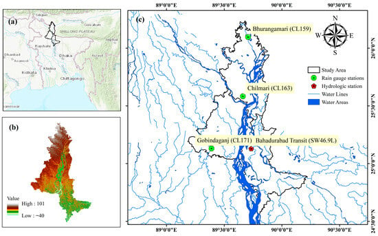
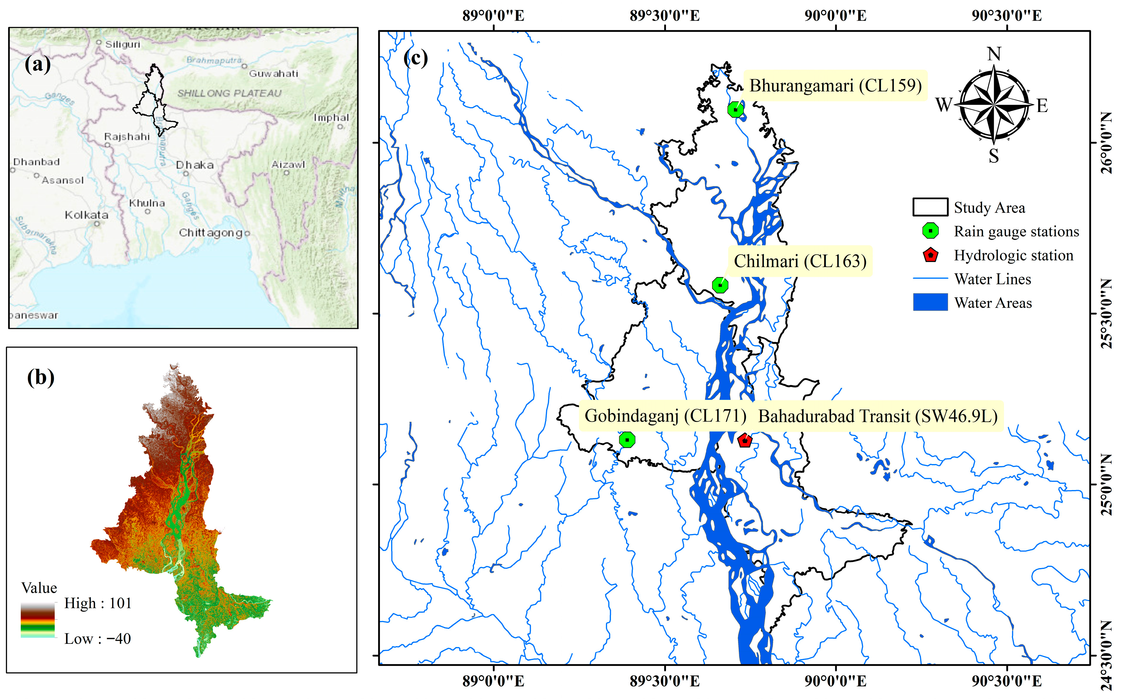
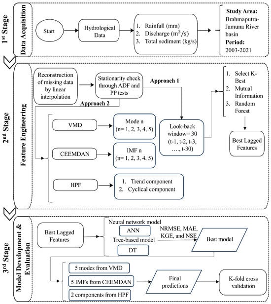
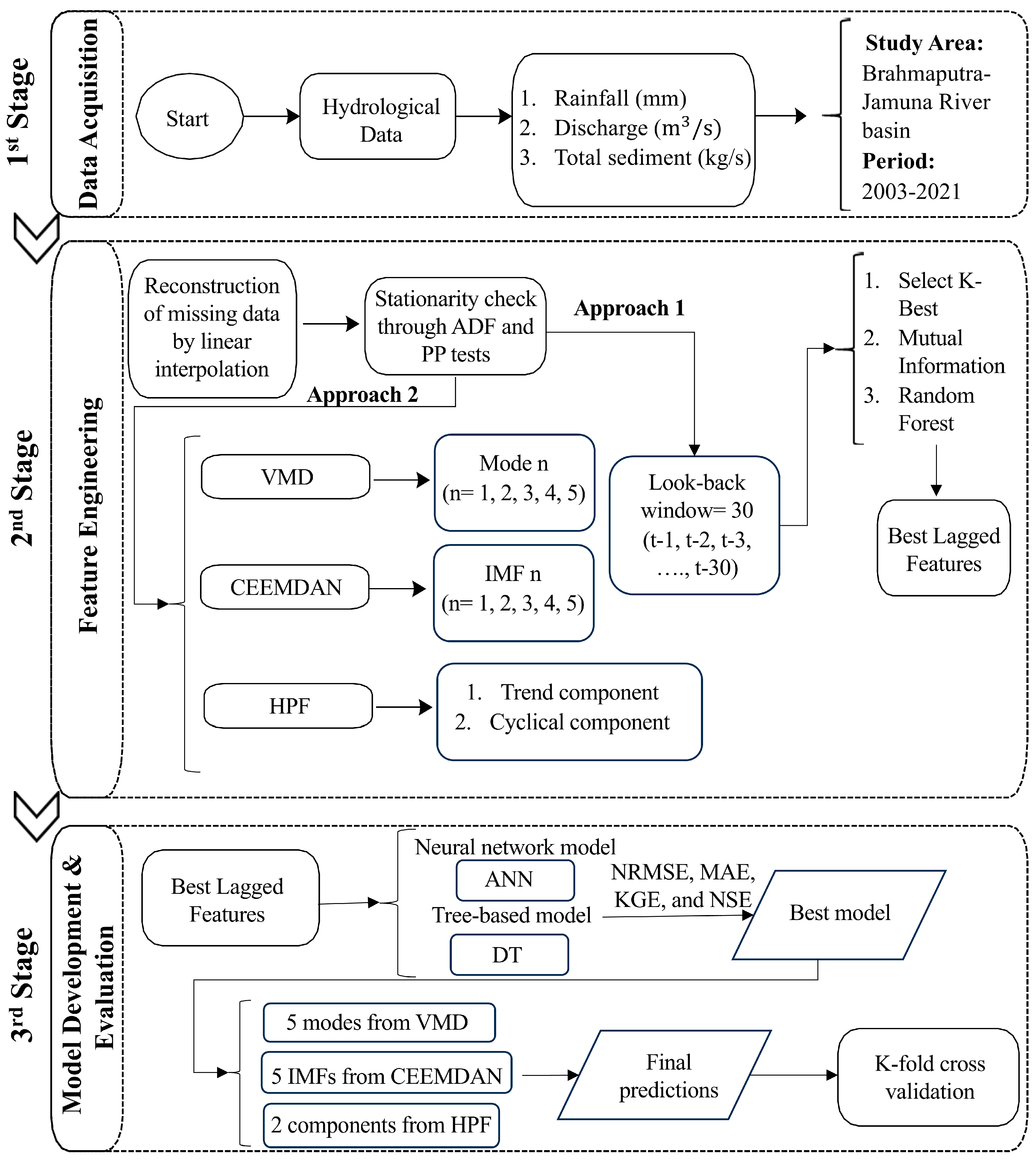
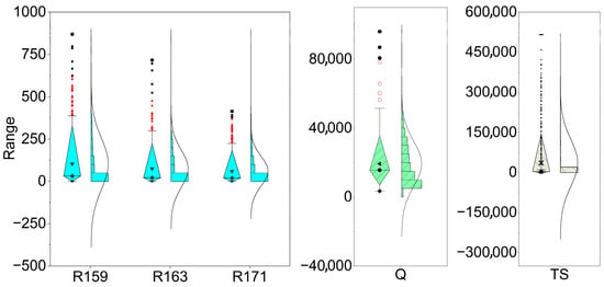
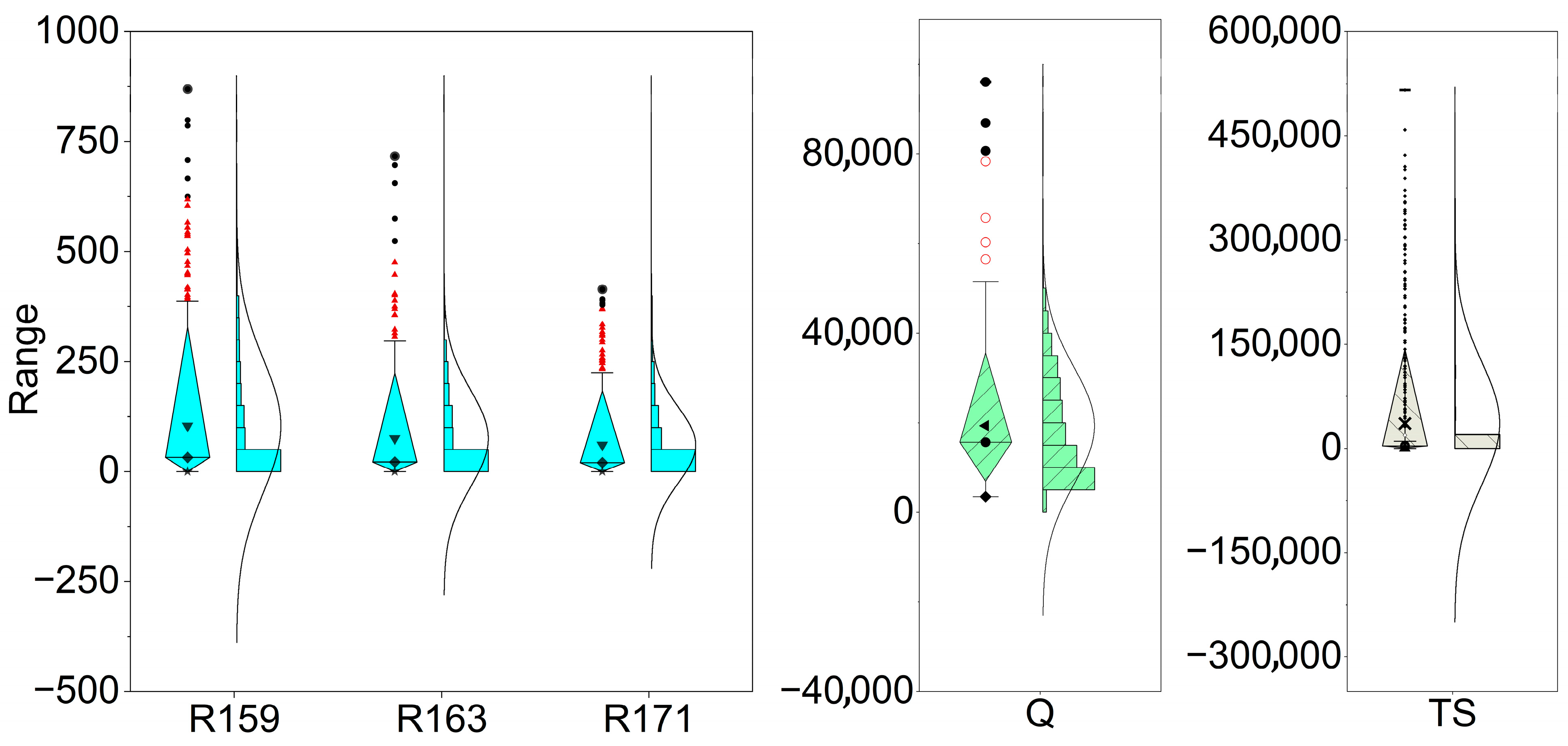
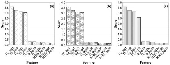
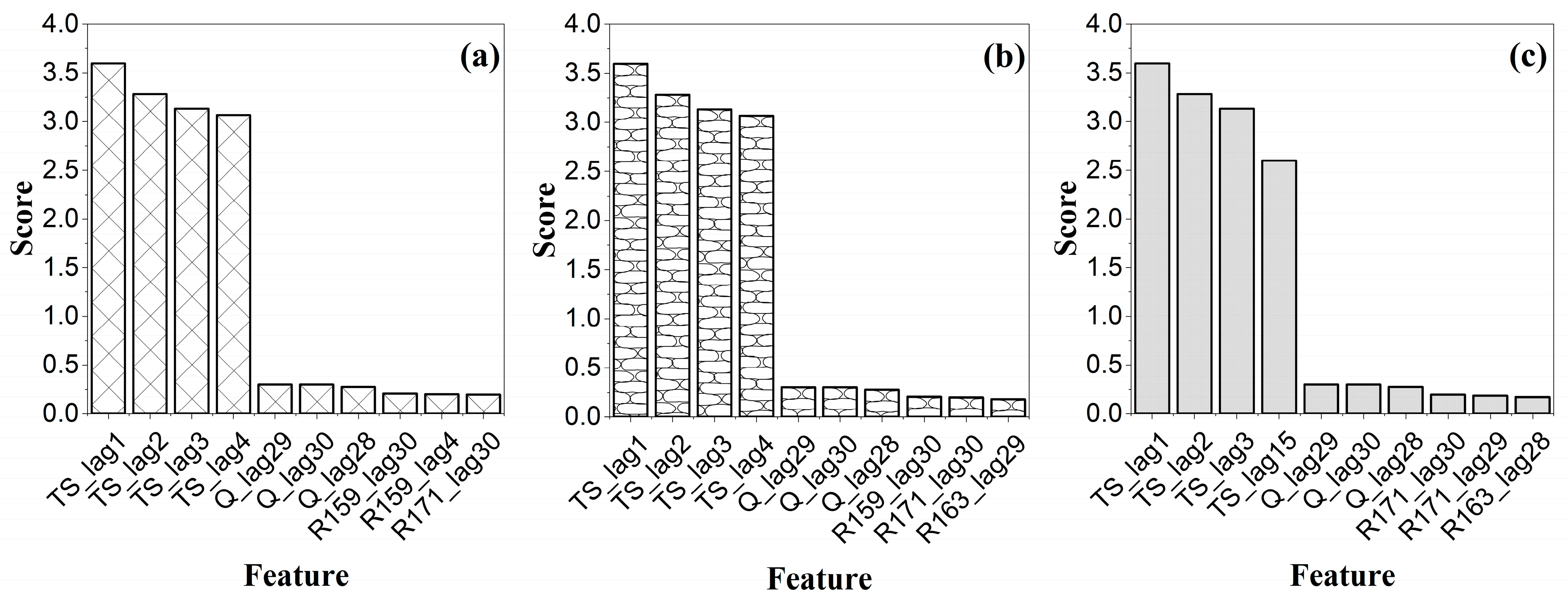
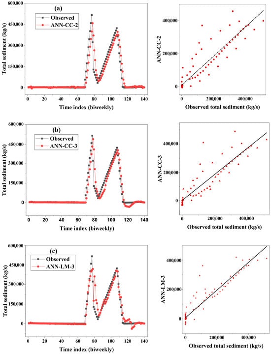
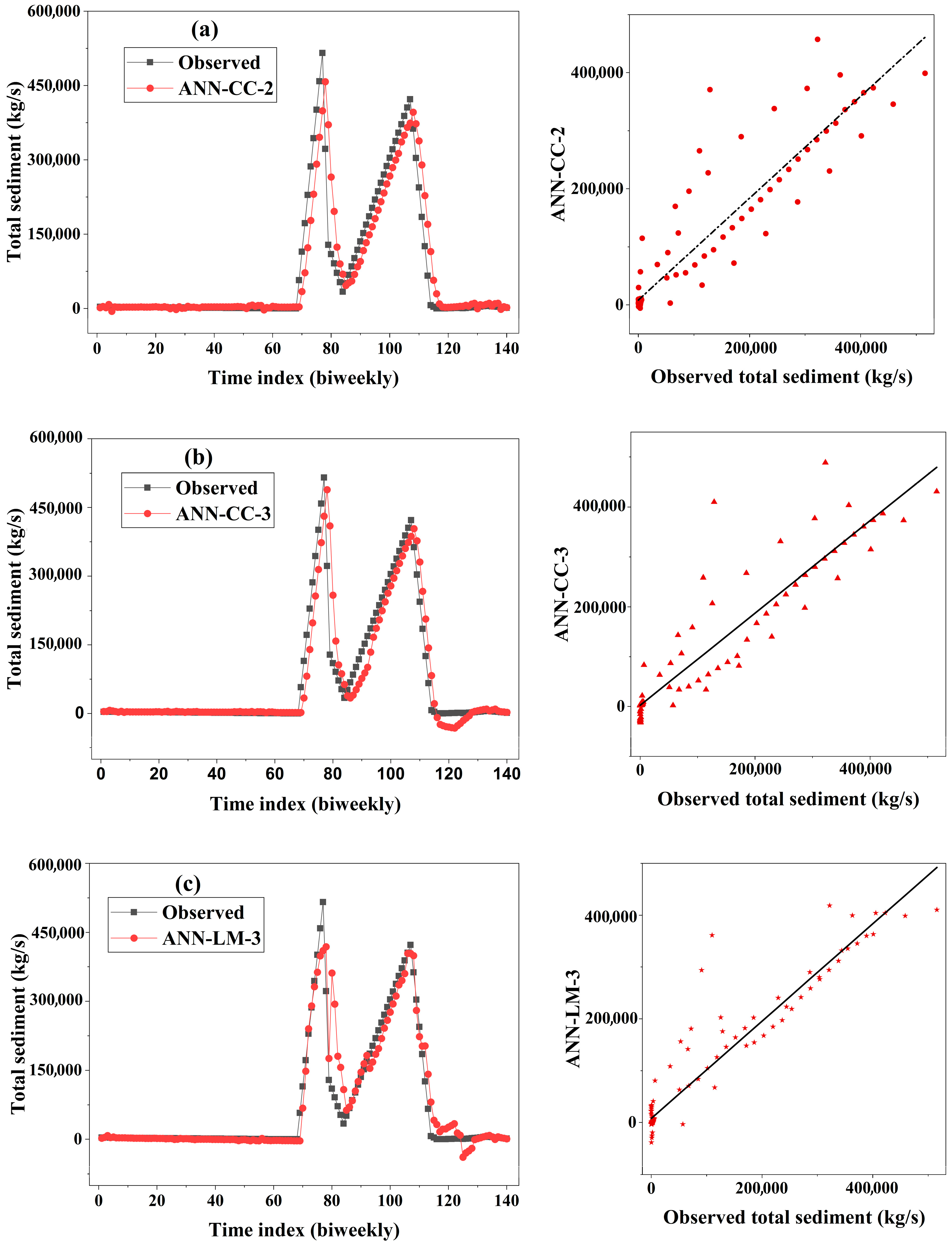
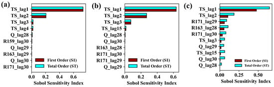
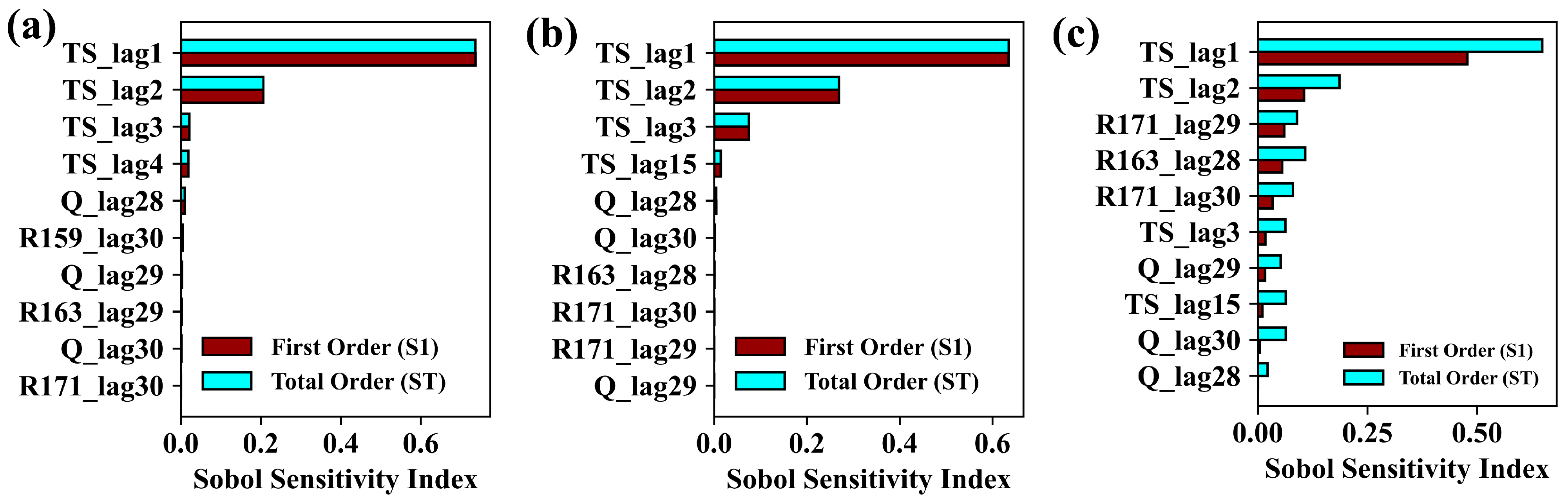
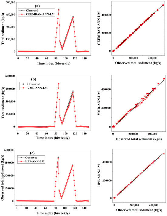
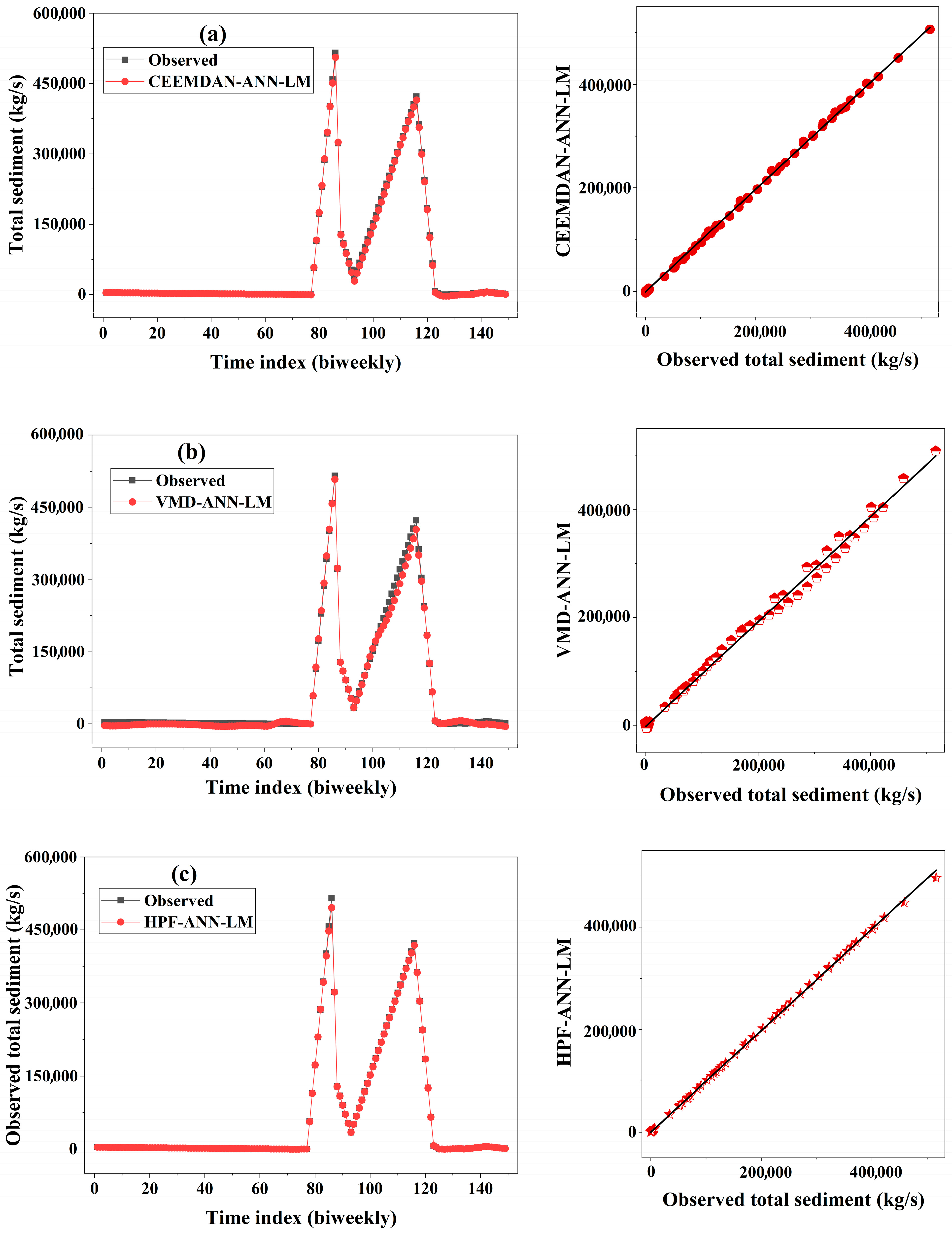
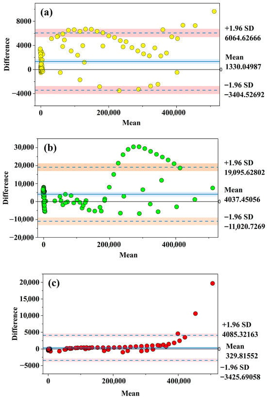
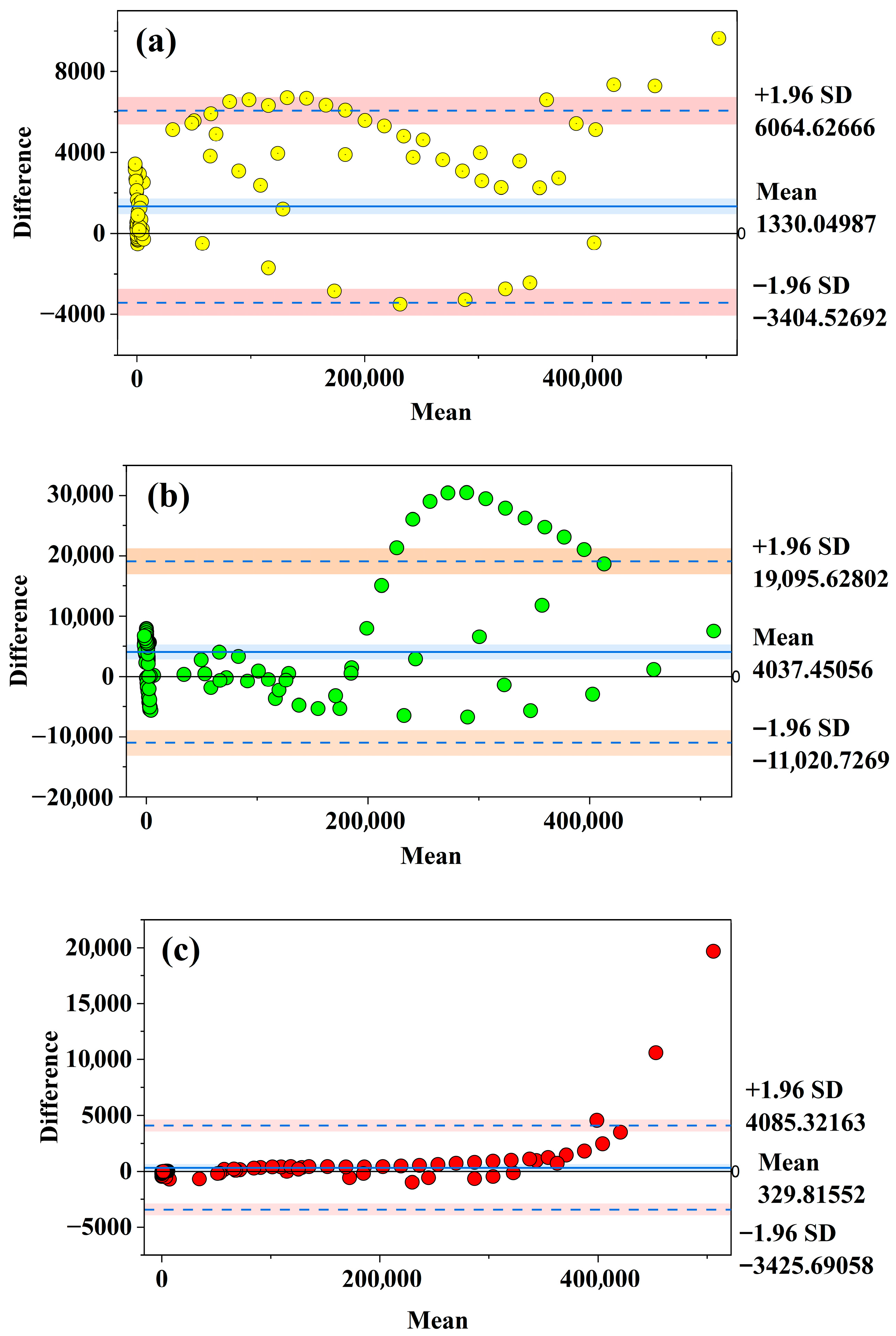
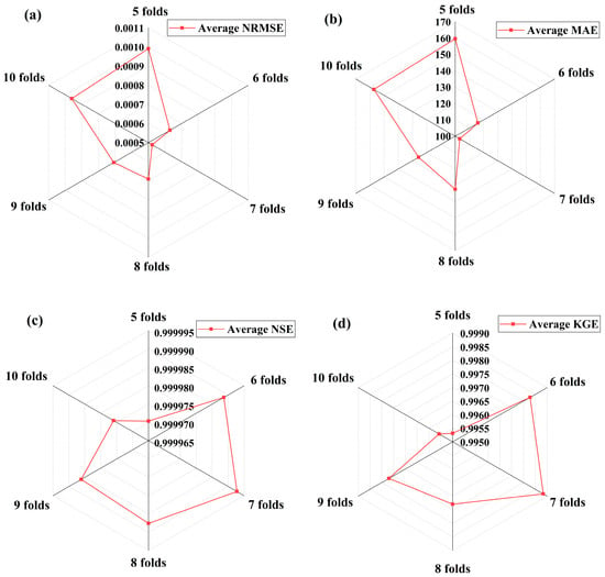
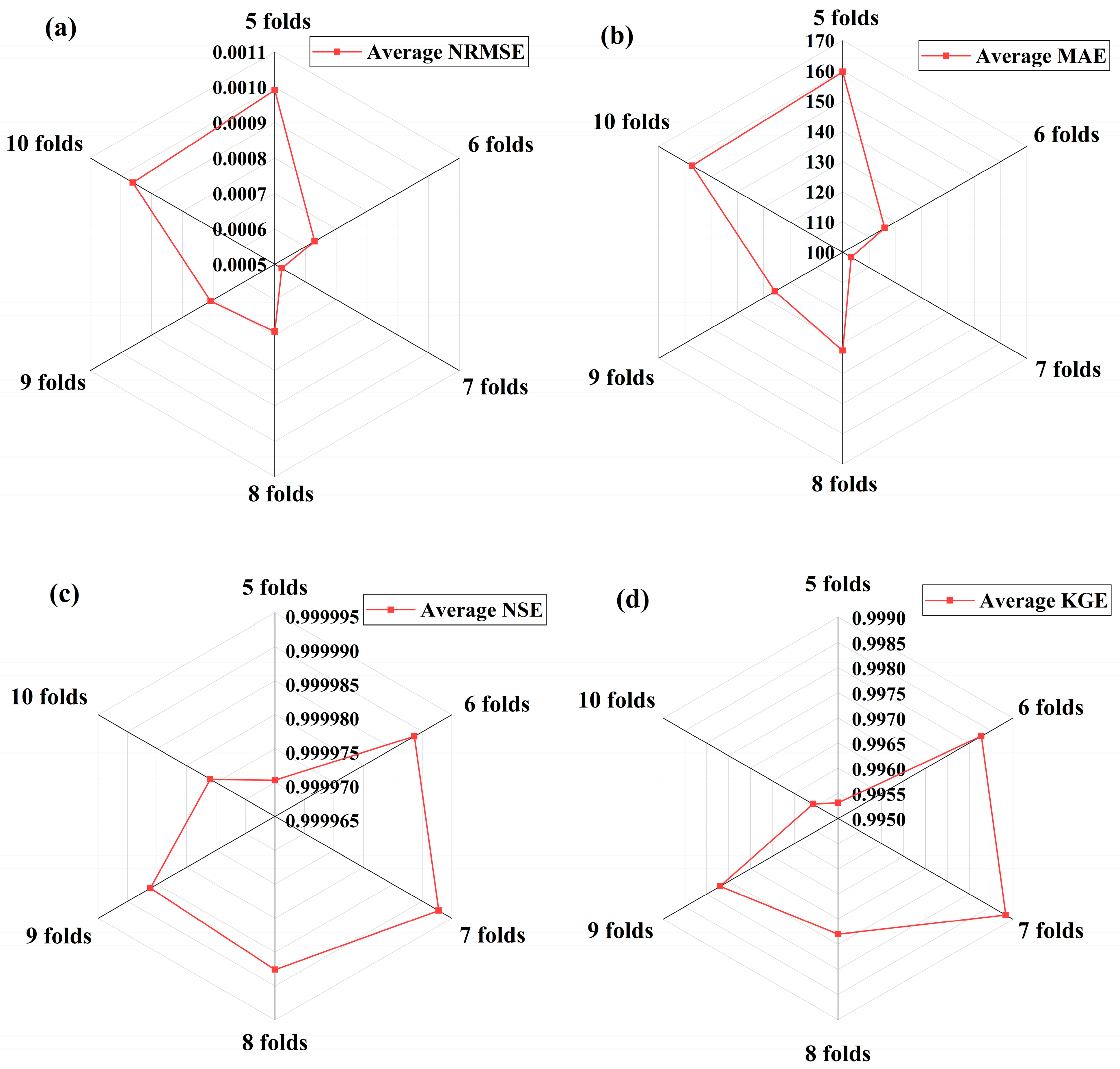

Disclaimer/Publisher’s Note: The statements, opinions and data contained in all publications are solely those of the individual author(s) and contributor(s) and not of MDPI and/or the editor(s). MDPI and/or the editor(s) disclaim responsibility for any injury to people or property resulting from any ideas, methods, instructions or products referred to in the content. |
© 2026 by the authors. Licensee MDPI, Basel, Switzerland. This article is an open access article distributed under the terms and conditions of the Creative Commons Attribution (CC BY) license.