


Abstract
Sea fog that lowers horizontal visibility below 1 km is a recurrent hazard to port operations and near-shore navigation, yet its objective, continuous short-range warning remains difficult. Using a microwave radiometer and a 35 GHz millimeter-wave cloud radar co-located at the Xiaoyangshan station near the Yangshan deep-water port, eastern China, supervised by a continuous minute-resolution visibility ground truth (about 0.65 million records, 2025–2026), we develop a calibrated probabilistic sea-fog nowcasting model for lead times of 0–3 h. Under strict date-grouped cross-validation—in which neither the input window nor any forecast label crosses a fold boundary—and at the operationally realistic fog base rate of ∼1.9%, the model attains a fog-state ROC-AUC of 0.95–0.96 across lead times and an onset-AUC of about 0.94 at the 3 h lead. After out-of-group isotonic calibration the output probabilities are reliable (expected calibration error 0.007), and a single-stage alarm reaches an event hit rate of 0.84 over the 2026 hold-out period—a figure that is unchanged under a strictly out-of-time protocol in which the model, the calibrator, and the alarm parameters are all frozen on data through 2025—with a median first alert about 3.1 h before fog onset. A compact near-surface scalar model already saturates discrimination; adding vertical profiles and radar microphysics through a mask-aware fusion network yields only a small, statistically non-significant gain, indicating that independent fog events, not model capacity, limit further improvement. The scheme is lightweight, locally deployable, and can be re-evaluated as observations accumulate.
1. Introduction
Sea fog is a weather phenomenon occurring over the sea or in the lower atmosphere of coastal areas, in which suspended water droplets or ice crystals reduce the horizontal visibility to below 1 km; by formation mechanism it is mainly classified into advection (cooling) fog and radiation fog [1]. Its formation and maintenance are jointly controlled by the advection of warm, moist air, long-wave radiative cooling at the fog top, and turbulent mixing within the boundary layer [2]. Modulated by air–sea interaction, sea fog exhibits pronounced seasonal and regional characteristics over the Yellow Sea, the East China Sea, and other waters [3,4]. Because of its abrupt onset, strong locality, and rapid life cycle, sea fog poses major safety risks to port loading and unloading, channel transit, and near-shore navigation, and the objective analysis and short-range nowcasting of the associated near-shore visibility have long been difficult problems for both observation and forecasting [5,6].
Satellite remote sensing can provide large-area, near-real-time monitoring of sea fog, but it struggles to observe the low-level fog beneath higher cloud layers when obscured, and its limited spatio-temporal resolution renders it inadequate for capturing abrupt, localized, thin sea-fog layers [7,8,9]. By contrast, ground-based remote sensing (millimeter-wave cloud radar, microwave radiometer, and ceilometer) offers high temporal resolution and near-surface detection capability, enabling continuous observation of the fog life cycle [10], and thus constitutes an important complement to satellite observation.
Millimeter-wave (Ka/W-band) cloud radars, with their short wavelengths and sensitivity to Rayleigh scattering from small cloud and fog particles, can detect non-precipitating clouds, weak precipitation, and the vertical structure of fog, and have become an effective means of vertical cloud and fog sounding [11,12,13]. For fog detection in particular, studies have used ground-based radar to relate the reflectivity of the fog layer to visibility [14], and have used W-band radar observations to improve fog forecasting and model diagnosis [15]. In recent years, applications of millimeter-wave radar to sea-fog observation have expanded further: some studies have mounted a 94 GHz radar on an unmanned surface platform to retrieve sea-fog microphysics and visibility [16], while others have combined scanning millimeter-wave radar with machine learning for near-shore sea-fog identification, achieving very high accuracy [17]. Microwave radiometers, in turn, passively retrieve profiles of boundary-layer temperature, water vapor, and liquid water, as well as the integrated liquid water path (LWP); they are sensitive to near-surface water-vapor changes and support long-term continuous observation, playing a significant role in fog monitoring and mechanistic studies [18,19,20]. At the methodological level, machine learning has been widely applied to the detection and forecasting of fog and low visibility, and has been systematically reviewed in recent years [21].
Nevertheless, two prominent problems persist for operationally oriented short-range sea-fog warning. First, most machine-learning studies adopt random splitting and near-balanced sampling, which introduce temporal-autocorrelation leakage and base-rate distortion, so that the high metrics reported can hardly represent the truly attainable performance. Second, there is a lack of nowcasting models that are supervised by a continuous visibility ground truth and are probabilistically calibrated. To address these gaps, we propose, based on the co-located MWR and MMCR at the Xiaoyangshan coastal station adjacent to the Yangshan deep-water port, a calibrated probabilistic sea-fog nowcasting model. Our main contributions are: (1) supervised by a continuous, minute-resolution visibility ground truth and evaluated under date-grouped leakage prevention, we construct a nowcasting model that outputs 0–3 h fog probabilities and onset discrimination, achieving high discriminative power (ROC-AUC 0.95–0.96); (2) through out-of-group isotonic calibration, we provide reliable fog probabilities and, via a single-stage alarm, an attainable operating point for operations (hold-out hit rate 0.84, median first alert about 3.1 h ahead); (3) we design a mask-aware radar–radiometer fusion network that degrades gracefully under missing radar, and show that a compact near-surface scalar model already saturates discrimination—the added vertical and radar structure yields only a small, statistically non-significant gain in the near-saturated hard regime, indicating that the bottleneck is the number of independent fog events rather than model capacity.
2. Materials and Methods
2.1. Study Site and Instruments
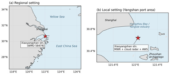
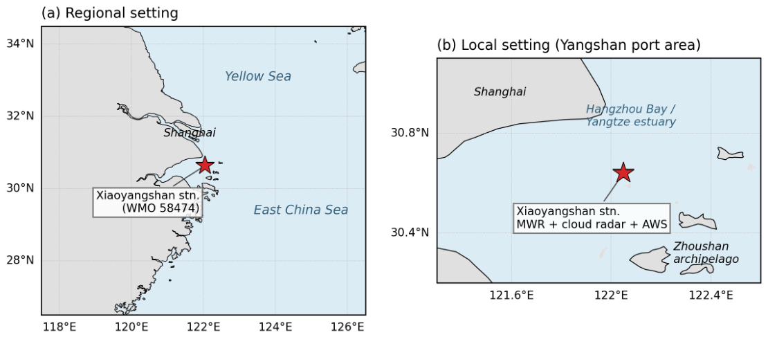
This study is based on the Xiaoyangshan National Basic Meteorological Station (WMO station 58474; 122.05° E, 30.64° N), located on Xiaoyangshan Island adjacent to the Yangshan deep-water port area of Shanghai, at the northwestern edge of the East China Sea (Figure 1). The surrounding waterway carries dense container traffic, so low-visibility episodes at this site directly constrain port scheduling and channel transit. The station hosts a co-located millimeter-wave cloud radar and a microwave radiometer—an active and a passive remote-sensing instrument—enabling coordinated, continuous observation of the low-level cloud and fog structure.
Figure 1.
Location of the Xiaoyangshan National Basic Meteorological Station (WMO 58474; 122.05° E, 30.64° N). (a) Regional setting on the East China Sea coast; (b) local setting of the station on Xiaoyangshan Island adjacent to the Yangshan deep-water port, with the co-located microwave radiometer, millimeter-wave cloud radar, and automatic weather station (visibility sensor).
The millimeter-wave cloud radar is an all-solid-state pulsed Doppler system with single-transmit dual-receive, operating at 35 GHz ± 500 MHz in a vertically pointing mode. Its range resolution is 30 m, its temporal resolution is ≤1 min, and its detection blind zone is ≤150 m. The radar’s Level-1 products include the reflectivity factor Z, radial velocity V, spectral width W, and linear depolarization ratio (LDR); the Level-2 products include the cloud-base height and cloud-top height [11,12].
The microwave radiometer is a TK001 ground-based system, a passive instrument certified for operational use by the China Meteorological Administration, which retrieves atmospheric states by receiving the brightness temperatures of the 22 GHz water-vapor absorption band and the 60 GHz oxygen absorption band [22]. Its CP profile product comprises 83 layers over the 0–10 km height range at a temporal resolution of once per 2 min, including profiles of temperature, water-vapor density, relative humidity, and liquid water content, together with the integrated water vapor, integrated cloud liquid water (i.e., LWP), cloud-base height, and surface temperature, humidity, and pressure [18,19,23]. The manufacturer-specified retrieval accuracies (root-mean-square errors) are ≤1.8 K for the tropospheric temperature profile (≤1.0 K within the boundary layer), ≤15% for the relative-humidity profile, ≤0.8 g m−3 for the water-vapor-density profile, and ≤4 mm for the integrated water vapor [22]. Table 1 summarizes the specifications of the two instruments.
Table 1.
Specifications of the two co-located ground-based remote-sensing instruments at the Xiaoyangshan station.
2.2. Data and Labels
The microwave radiometer provided about 686 days of continuous 2 min CP profiles (T/RH/LWC/VD, 83 layers) during 2024–2026; the millimeter-wave cloud radar archive comprised about 447 complete observation days (January 2025–May 2026, Z/LDR profiles); and the minute-resolution visibility from the co-located automatic weather station (1 January 2025 to 27 March 2026, about 0.65 million records, 0.01% missing) served as the continuous ground truth. Following the WMO standard, horizontal visibility < 1 km was taken as fog, and from the continuous visibility (10 min visibility < 1 km, persisting ≥10 min, with segment-mean visibility < 1 km used to remove instantaneous spikes) we reconstructed 71 fog events as the modeling gold standard; verification showed that this reconstruction fully covers the station’s manual fog records (41/41, no false positives) and additionally recovers about half of the genuine low-visibility events missed by manual curation, thereby ensuring accurate and complete labels.
Sample construction proceeds in a cascade that we summarize in Table 2 so that the various sample counts are unambiguous. The radiometer 2 min feature table contains 368,354 samples; restricting to centers with a contiguous one-hour look-back that lies entirely within the center’s date group leaves 309,199 multi-lead center samples (used for the multi-lead discrimination of Section 3.1); in addition, a forecast target whose valid time falls outside the center’s date group is masked for that horizon, so that neither the input window nor any label ever crosses a cross-validation group boundary (Section 2.4). Throughout we keep the realistic fog base rate of about 1.6–1.9% at the 2 min sample level, depending on the subset (Table 2; no near-balanced resampling, to remain faithful to operations). The co-located radar–radiometer joint modeling subset comprises 25,426 records, of which 22,289 have a valid visibility label (about 87% also carry a radar profile, with entirely missing radar segments marked by a mask); within it, the near-saturated hard regime () contains 3305 samples.
Table 2.
Data-flow cascade from raw observations to the modeling subsets, with the fog base rate of each subset and the analysis it feeds.
The seasonal distribution of the 71 reconstructed fog events (Table 3) reflects the local sea-fog climatology at the northwestern edge of the East China Sea: spring (MAM) dominates with 39 events, followed by winter (DJF, 19) and early summer (JJA, 13), while no event with visibility below 1 km occurred in autumn (SON) during the study period. Discrimination is stable across the seasons that contain fog—the seasonal ROC-AUC ranges from 0.94 (JJA) to 0.97 (DJF) with overlapping confidence intervals, and the monthly AUC stays within 0.85–0.99 over the ten months that contain both classes—indicating that the model does not merely average over season-specific mechanisms; the autumn gap and the single-fog-season depth of the record are discussed as limitations in Section 4.4.
Table 3.
Seasonal distribution of the 71 reconstructed fog events and seasonal performance (fog-state OOF ROC-AUC with day-grouped bootstrap 95% confidence intervals; event hit rate under the frozen alarm parameters). No fog event occurred in SON during the study period, so seasonal AUC and hit rate are undefined there.
2.3. Models and Framework
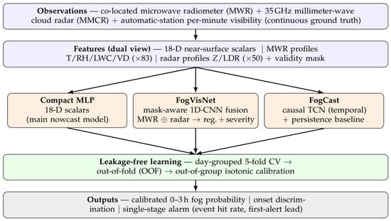
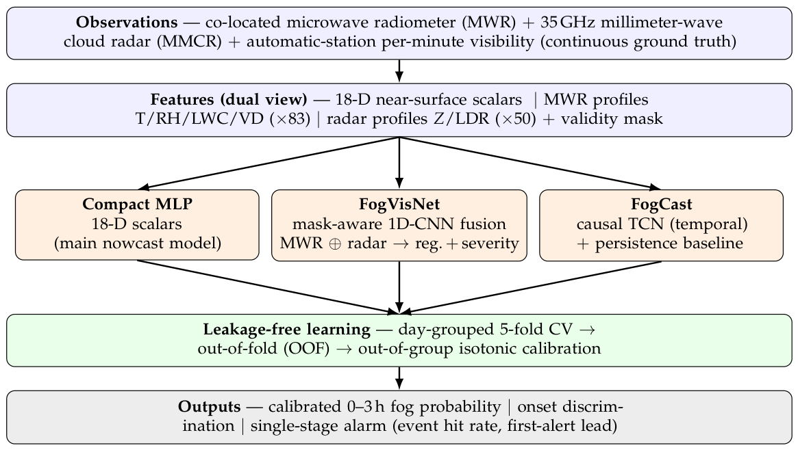
Our framework characterizes the atmospheric state through a dual-view representation and a family of models of increasing complexity, all trained and evaluated under a single leakage-free protocol (Figure 2). The first view consists of low-dimensional, physically interpretable near-surface scalars that summarize the thermodynamic and humidity state; the second consists of the full vertical profiles—radiometer thermal/moisture profiles and radar microphysical profiles—that resolve structural detail. By spanning models from a compact scalar classifier to multi-source deep networks, the framework simultaneously delivers an operational nowcast and lets us assess whether added structural or temporal complexity improves discrimination.
Figure 2.
Overview of the calibrated probabilistic sea-fog nowcasting framework. Co-located ground-based remote-sensing observations and continuous visibility ground truth are mapped into a dual-view feature set (near-surface scalars and vertical profiles). Three models of increasing complexity—a compact scalar MLP (the main nowcast model), the mask-aware radar–radiometer fusion network (FogVisNet), and the causal temporal network (FogCast)—are trained and calibrated under a single leakage-free protocol (day-grouped cross-validation, out-of-fold prediction, and out-of-group isotonic calibration) and produce calibrated multi-lead fog probabilities, onset discrimination, and a single-stage operational alarm. Arrows indicate information flow; colors distinguish observations and features (blue), models (orange), evaluation and calibration (green), and outputs (gray).
2.3.1. Compact Scalar MLP (Main Model): What and Why
The main model is a compact multilayer perceptron (MLP) acting on 18 physically interpretable near-surface scalars—RH and LWC at several near-surface heights, cloud-base height, LWP, integrated water vapor, and surface temperature/humidity/pressure—with logistic regression (LR) as a linear reference baseline. Why this design: sea-fog formation is governed by near-surface saturation, a shallow temperature inversion, and increasing low-level liquid water—an inherently low-dimensional signal. A compact model captures this signal directly while resisting over-fitting on the rare positive class (a realistic base rate of only 1.6–1.9%), and it remains cheap to deploy and to retrain as local observations accumulate.
2.3.2. Mask-Aware Radar–Radiometer Fusion (FogVisNet): What and Why
FogVisNet jointly exploits the radiometer thermodynamic profiles and the radar microphysical profiles through a mask-aware mid-fusion architecture. Each modality has a parallel 1-D convolutional encoder [24] along height (radiometer T/RH/LWC/VD × 83 layers; radar Z/LDR × 50 layers); every encoder receives the standardized profile together with a binary validity-mask channel, and average + max pooling produces a per-modality embedding. The two embeddings are concatenated with a radar-availability flag and passed through an MLP to two heads: a log-visibility regression head and a 4-class severity head ({<500, 500–1000, 1000–10,000, ≥10,000 m}). Why this design: the goal is to test whether the high-dimensional vertical structure and radar microphysics add discrimination beyond the scalars—especially in the near-saturated hard regime where the radiometer humidity signal saturates. Making “missing” an explicit input channel is essential because the radar has a ≤150 m near-surface blind zone and is entirely absent in ∼13% of samples; randomly zeroing the radar branch during training further lets the network degrade gracefully to a radiometer-only model at inference.
2.3.3. Causal Temporal Network (FogCast) and Baseline: What and Why
FogCast is a causal temporal convolutional network [25] applied to a look-back window of 2 min scalar features; it is left-padded only and never uses future samples, emitting a fog probability for each lead time. Why this design: it tests whether the temporal trajectory of the precursors improves onset lead beyond the instantaneous state, while the strict causality guarantees that the reported lead times contain no future-information leakage and are therefore operationally honest. A persistence baseline—extrapolating the current fog state forward—provides the meteorological reference against which all models are judged.
2.3.4. Multi-Lead Nowcasting and Onset Task
For each 2 min center sample we predict the probability that the 10 min mean visibility is <1 km at lead time min, yielding multi-lead fog probabilities; the onset task restricts the evaluation to currently non-fog samples (vis ≥ 1 km) and asks whether fog forms h minutes later.
2.3.5. Class-Imbalance Handling
We adopt cost weighting based on the inverse of class frequency [26] (weighted cross-entropy for the deep models/binary cross-entropy with pos_weight; class_weight=’balanced’ for the scalar baseline), and train with cosine annealing and early stopping on the validation-set macro-F1.
2.4. Evaluation and Probability Calibration
2.4.1. Date-Grouped, Leakage-Free Cross-Validation
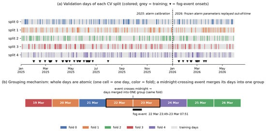
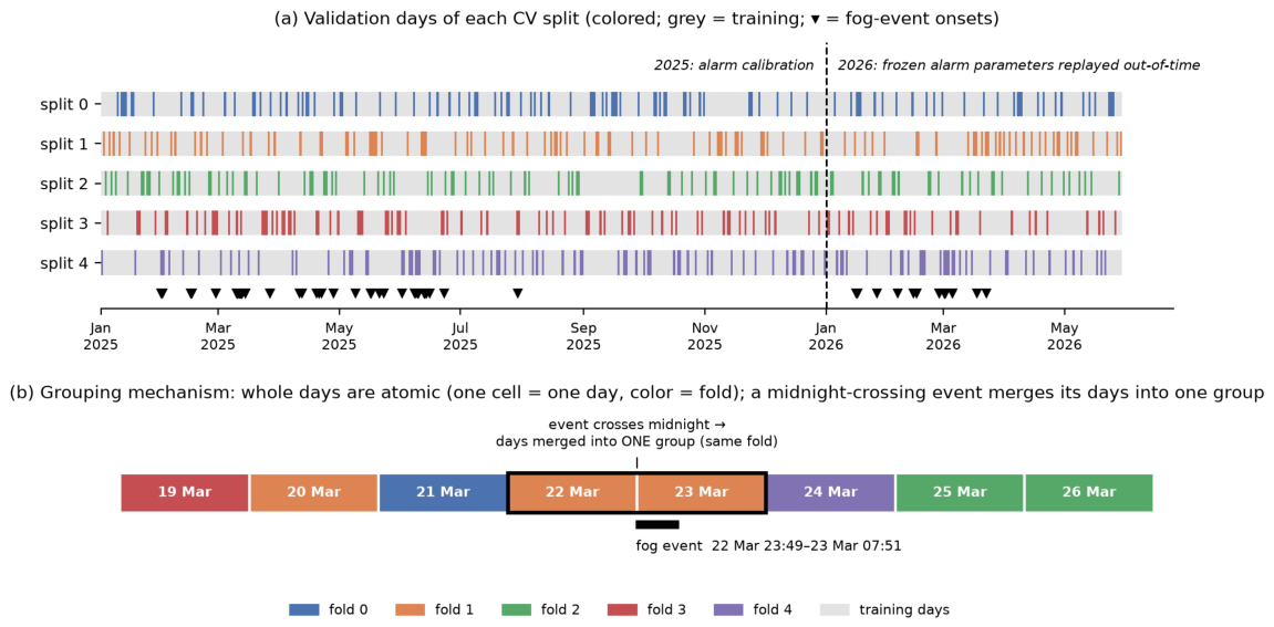
We uniformly adopt 5-fold cross-validation grouped by calendar day (Beijing time), ensuring that samples from the same date never span the training and validation sets. The groups are built in two steps: each calendar day forms one group, and all days covered by a fog event that crosses midnight are chain-merged into a single group, so that no fog event is ever split across folds. The resulting 438 day groups are assigned to the five folds by a greedy balancing rule—groups are sorted by their fog-sample count and each is assigned to the currently lightest fold—which keeps the fog base rate of every fold close to the overall 1.8–1.9% while each fold holds roughly one-fifth of the day groups. For the multi-lead task, the one-hour look-back window is required to lie entirely within the center’s date group (12,656 window-crossing centers are discarded), and a forecast target whose valid time falls in a different date group is masked for that horizon (from 6542 targets at min to 39,287 at min); consequently, neither an input window nor a training or evaluation label ever crosses a fold boundary. The standardization statistics for each fold are computed solely from that fold’s training set. Figure 3 visualizes the temporal layout of the folds, the 71 fog events, and the 2025/2026 alarm calibration/hold-out split.
Figure 3.
Date-grouped 5-fold cross-validation. (a) Validation days of each of the five cross-validation splits (one row per split; colored bars mark the days held out for validation in that split, grey the training days; triangles mark the onset times of the 71 reconstructed fog events). Each fold samples the full record, so every split validates on all represented seasons. The dashed line separates the 2025 alarm-calibration period from the 2026 period on which the frozen alarm parameters are replayed out-of-time. (b) The grouping mechanism, illustrated on a real week: whole calendar days are atomic (one cell per day, color = fold), and a fog event that crosses local midnight merges the days it covers into a single group (bold outline), so no event is ever split between training and validation.
2.4.2. Probability Calibration
The raw probability of each 2 min sample is taken from the out-of-group out-of-fold (OOF) predictions, on top of which we perform out-of-group isotonic-regression calibration [27] (the calibration mapping for fold k is fitted only from the remaining folds). Reliability is assessed via the reliability curve [28], the Brier score [29], and the expected calibration error (ECE).
2.4.3. Metrics
Discriminative power is measured by the threshold-independent ROC-AUC and, because the fog base rate is low (∼1.9%) and the ROC-AUC is then insensitive to the false-alarm burden, by the area under the precision–recall curve (AUPRC), whose no-skill reference equals the base rate. The contingency-table metrics include the probability of detection , the false alarm ratio (equivalently , not ), the critical success index , and the macro-averaged F1 (macro-F1):
The expected calibration error aggregates the gap between predicted confidence and empirical frequency over B probability bins:
where is the set of samples falling in bin b, is the empirical fog frequency, and is the mean predicted probability. The isotonic-regression calibrator learns a non-decreasing mapping g that minimizes subject to monotonicity, fitted on out-of-group OOF probabilities and applied to the held-out fold.
2.4.4. Uncertainty Quantification and Model Comparison
Because consecutive 2 min samples are strongly autocorrelated, sample-level asymptotic tests that assume independent observations (e.g., DeLong’s test for correlated ROC curves) would substantially underestimate the variance of every metric. Unless otherwise stated, the confidence intervals reported in this paper are therefore day-grouped bootstrap intervals: whole date groups are resampled with replacement () and the metric is recomputed on each resample, which preserves the within-day dependence structure and matches the grouping unit of the cross-validation design. Model comparisons use the same procedure in paired form—the metric difference between two models is recomputed on each day-group resample—complemented by a fold-level sign test and by Cohen’s d computed on the five paired fold differences as an effect-size measure. Event-level proportions (alarm hit rates) additionally carry Wilson score intervals, which are appropriate for the small event counts (52 and 19).
2.4.5. Single-Stage Alarm
The alarm logic operates on the OOF fog probability and is defined by three parameters—an entry threshold, the number of consecutive entry frames, and an exit hold duration. The threshold is not selected by Youden’s index or F1 optimization; instead we use a cost-based operational decision rule: over the 2025 calibration period only, the three parameters are grid-searched (entry thresholds taken as quantiles of the calibration-period probabilities; entry frames ; exit hold min) under the constraint of “minimizing the number of false-alarm episodes subject to an event hit rate ≥ 0.85,” which directly encodes the operational cost asymmetry between misses and false alarms. The winning triple (threshold at the ∼0.84 raw-probability level, 5 consecutive frames, 60 min exit hold) is then frozen and replayed over the 2026 hold-out period; a sensitivity analysis of the hit-rate/false-alarm trade-off as the entry threshold is varied around the frozen operating point is given in Figure S3 of the Supplementary Materials. An alarm episode that overlaps the event window is counted as a hit, and the first-alert lead is the difference between the start of the first overlapping alarm episode and the event start (negative denotes earlier). Two conventions should be noted. First, in replay scoring an episode’s start is the first sample of the qualifying consecutive run; in real time the entry condition is confirmed only after all 5 consecutive frames, so the operational first alert is issued min later than the replay start—negligible relative to the multi-hour leads reported, but stated here for operational fidelity. Second, an alarm episode may begin earlier than the 2 h pre-onset credit window and persist into it (the model responds to precursor conditions that precede the event by several hours); such episodes are counted as hits and their full lead is reported, which is why median leads can exceed 2 h.
3. Results
3.1. Multi-Lead Discrimination Performance
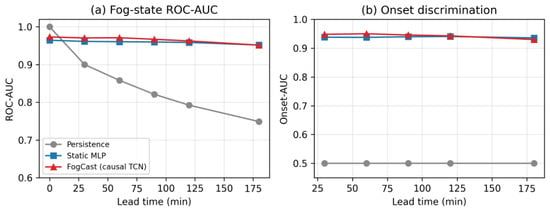
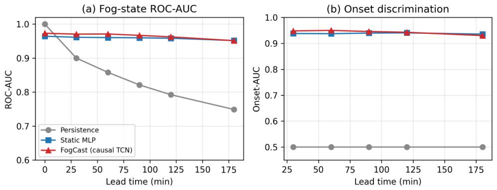
Under the date-grouped 5-fold OOF protocol with the boundary-tightened sample construction of Section 2.4, over 309,199 2 min center samples, and at a realistic fog base rate of ∼1.9%, the model maintains high discriminative power across all lead times (Table 4; Figure 4): the fog-state ROC-AUC decays gently from 0.965 at to 0.952 at 3 h, and is consistently and markedly superior to the persistence baseline (1.00 → 0.749) throughout. For the onset discrimination of “currently clear → future fog,” the onset-AUC is about 0.94 across 30–180 min (0.935 at 3 h), indicating that the model possesses an onset-warning capability several hours in advance. The causal temporal network (FogCast) attains slightly higher AUCs than the static-feature model at short leads (e.g., 0.973 versus 0.965 at ; onset-AUC 0.948 versus 0.938 at 30 min), with the two models converging by 3 h; the gap never exceeds 0.010, so the near-surface thermodynamic/humidity features at a single time already robustly support multi-lead discrimination, with the recent trajectory adding a small short-lead refinement.
Table 4.
Fog-state discrimination ROC-AUC at each lead time (date-grouped 5-fold OOF under the boundary-tightened protocol of Section 2.4; persistence/static MLP/causal-temporal FogCast).
Figure 4.
Fog-state discrimination ROC-AUC (a) and onset-AUC (b) at each lead time under the boundary-tightened protocol: persistence baseline, static MLP, and causal-temporal FogCast. The nowcasting models are markedly superior to persistence throughout, and the 3 h onset-AUC still reaches about 0.93–0.94.
Because the ROC-AUC is optimistic under the low fog base rate, we additionally report the AUPRC and day-grouped bootstrap () 95% confidence intervals for the main model (Table 5). The ROC-AUC confidence intervals are narrow and lie well above 0.9 at every lead (e.g., 0.964 [0.952, 0.979] at ), and the intervals of neighboring lead times overlap substantially, so differences between adjacent leads are not resolvable at the current event count—only the contrast between and min approaches the interval width. The AUPRC decreases from 0.32 at to 0.25 at 3 h—about 13–17× the no-skill reference of 0.019—confirming substantial precision–recall skill well beyond chance; at the same time it makes explicit that, at a ∼1.9% prevalence, the per-sample precision is modest, which is why the operational warning is issued at the event level via the temporal alarm rather than per sample (Section 3.2).
Table 5.
Multi-lead discrimination of the main model (static MLP) at the operational base rate (∼1.9%), with day-grouped bootstrap () 95% confidence intervals, under the boundary-tightened protocol of Section 2.4. AUPRC is reported against its no-skill reference (equal to the base rate, ≈0.019); “lift” is AUPRC divided by the no-skill reference.
3.2. Probability Calibration and Single-Stage Alarm
At the per-sample level, choosing an operating threshold on the main model’s fog probability gives the contingency metrics in Table 6: a CSI-optimal point reaches POD 0.59 at FAR 0.67 (CSI 0.27), and a high-recall point reaches POD 0.93 at FAR 0.82. As anticipated from the AUPRC, the per-sample precision is modest at a ∼1.9% base rate; the operational value is therefore realized by aggregating the calibrated probabilities over time into event-level alarms, as follows.
Table 6.
Per-sample contingency metrics of the main model at (309,199 samples, base rate ∼1.9%) at two operating points on the OOF fog probability. FAR = 1 − precision.
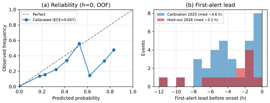
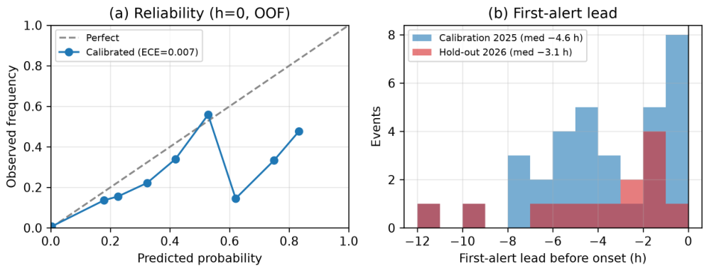
After out-of-group isotonic calibration, the model’s output fog probabilities agree closely with the empirical occurrence frequency (Figure 5, left; the reliability curve lies near the diagonal): the expected calibration error falls from 0.065 [95% CI 0.053, 0.079] (raw) to 0.007 [0.003, 0.014] after isotonic calibration, with a Brier score of 0.014 [0.009, 0.021] (10 equal-width bins; day-grouped bootstrap intervals throughout).
Figure 5.
Out-of-fold (OOF) probability reliability curve (, (a)) and the distribution of the single-stage alarm’s first-alert lead ((b), calibration/hold-out periods). The calibrated probabilities are close to perfectly reliable, and the median first alert is about 3.1 h ahead.
The single-stage alarm operates on the OOF fog probability with the parameters frozen over the 2025 calibration period (Section 2.4). Over the 2025 calibration period itself it hits 46/52 = 0.88 [Wilson 95% CI 0.77, 0.95]—a within-search figure, since the parameter grid was constrained to a hit rate on these events—and over the 2026 hold-out period it hits 16/19 = 0.84 [0.62, 0.95]; the median first alert is issued about 3.1 h ahead of onset (hold-out period, min [bootstrap 95% CI , ]; P25 /P75 min; about 4.6 h over the calibration period) (Figure 5, right). Two senses of “out-of-time” should be distinguished. In the pooled protocol above, the three alarm parameters never touched any 2026 information, while the underlying per-sample probabilities remain day-grouped out-of-fold over the pooled record (a 2026 sample is scored by a model that has never seen its own day group, though trained on other 2026 days). To verify that this distinction does not flatter the results, we additionally ran a strictly out-of-time deployment simulation: the classifier and the isotonic calibrator were fitted on data through 2025 only (the calibrator on inner day-grouped OOF pairs), frozen together with the alarm parameters, and run forward over 2026. Under this strict protocol the 2026 fog-state ROC-AUC is 0.951 (calibrated; 0.958 raw), the event hit rate is unchanged at 16/19 = 0.84, and the median first alert is min (≈2.6 h); the false-alarm burden rises from about 6 to about 12 episodes per month, reflecting the calibration shift that online re-calibration would absorb in operations. The hold-out false alarms of the pooled protocol are about six segments per month; for the most pronounced low-visibility false-alarm segments, a spot-check minute-resolution visibility review shows that most correspond to genuine low visibility of light/near fog (vis 1–5 km), indicating that a substantial fraction of the alarms fall near the fog/non-fog definitional boundary rather than being triggered spuriously. These results show that the model is not only highly discriminative but also probabilistically reliable—and that its hold-out skill survives a fully frozen, deployment-grade protocol—so that an operating point can be chosen directly according to the operational cost of misses and false alarms.
3.3. A Hold-Out Fog-Event Case Study
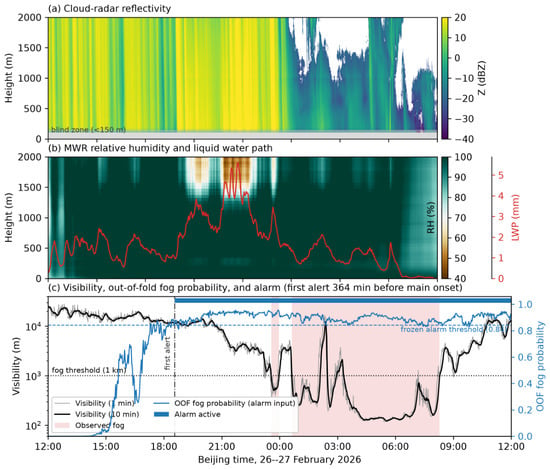
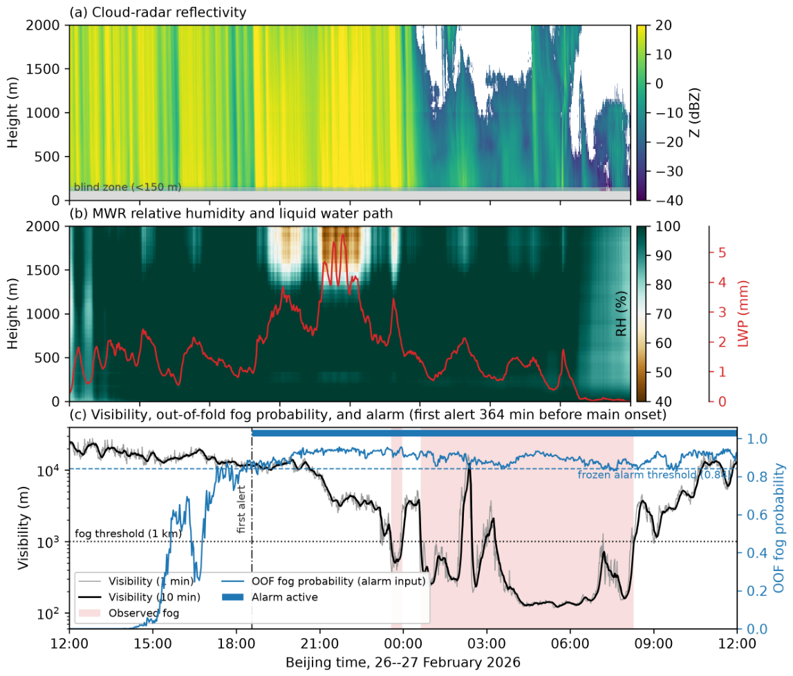
Figure 6 illustrates the behavior of the full chain—observations, probability, and alarm—on the longest fog event of the 2026 out-of-time hold-out period (27 February 2026, 00:38–08:17 Beijing time, minimum visibility 122 m), which was preceded by a brief fog patch just before midnight. The afternoon and evening of 26 February were dominated by light precipitation beneath a nearly saturated column: the cloud radar shows echo filling the lowest 2 km (reflectivity locally exceeding 10 dBZ), while the radiometer indicates relative humidity close to saturation below about 1.5 km and a liquid water path repeatedly exceeding 2 mm. As the precipitation weakened during the evening, visibility declined steadily from above 20 km; after fog onset the radar echo collapses to a shallower, weaker structure with intermittent drizzle, and the near-saturated state persists until the fog dissipates after sunrise.
Figure 6.
Hold-out case study of the 26–27 February 2026 fog event (Beijing time). (a) Millimeter-wave cloud-radar reflectivity (gates with a signal-to-noise ratio below 0 dB are masked for display; the gray band marks the ≤150 m blind zone). (b) Microwave-radiometer relative-humidity profile with the liquid water path (LWP, red). (c) One-minute and 10 min visibility (logarithmic scale), the out-of-fold (OOF) fog probability used by the alarm together with the frozen alarm threshold (dashed), alarm-active segments (top bar), and the observed fog segments (shading). The first alert was issued 364 min before the main fog onset.
The OOF fog probability (Figure 6c) rises through the evening and first satisfies the frozen alarm-entry condition at 18:34 Beijing time—364 min (about 6.1 h) before the main onset—while the observed visibility was still above 10 km. The alarm then remains continuously active through both fog segments and releases only after visibility has recovered, so the event is scored as a hit with a first-alert lead well above the hold-out median of about 3.1 h (Section 3.2). The case also illustrates the sensor division of labor discussed in Section 4.1: the radiometer-dominated near-surface saturation signal drives the early probability rise, while the radar documents the transition from precipitation to a shallow fog layer above its 150 m blind zone.
3.4. Model and Input Comparison and the Radar Gain in the Hard Regime
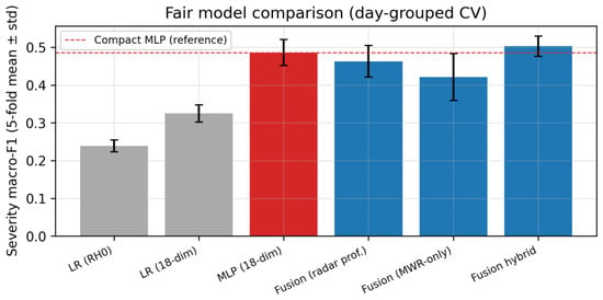
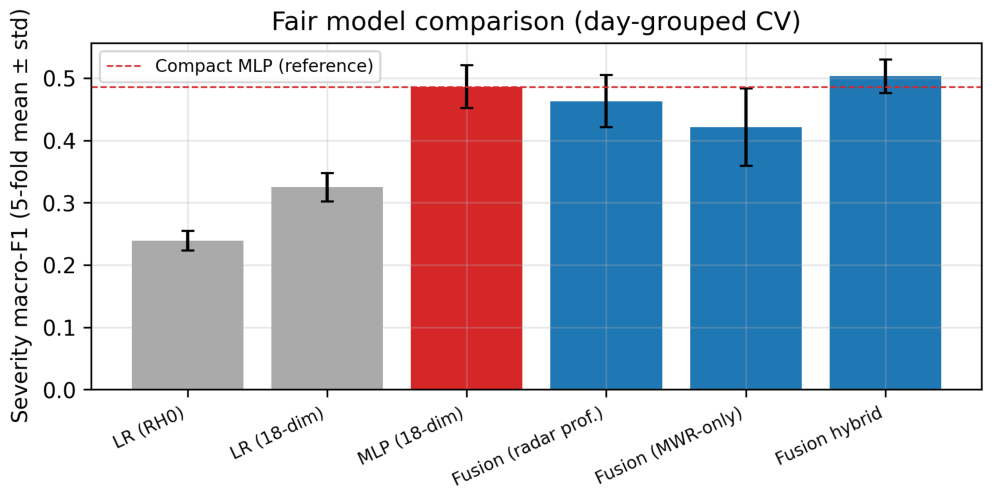
To examine the choice of model and input, we performed a fair comparison of the visibility-severity classification over 22,289 joint radar–radiometer samples (fog rate 5.2%, 438 date-grouped 5 folds) (Table 7; Figure 7). The compact scalar MLP (18-D) attained a fold-mean severity macro-F1 of 0.486 ± 0.034, and the hybrid model fusing profiles, radar, and scalars reached 0.503 ± 0.027; both are markedly superior to the linear baseline (LR 0.239–0.325). The results show that a compact model already attains robust performance; the improvement from introducing profiles and multi-source information is small and not statistically significant—the paired fold-level difference (hybrid − compact MLP) is macro-F1 (mean ± std over the five folds; sign-test ; Cohen’s ), and the paired day-grouped bootstrap 95% confidence interval of the pooled difference, , includes zero—so deployment can flexibly select according to cost. The modest effect size indicates that the non-significance reflects a genuinely small gain relative to the between-day variability, not merely a lack of statistical power at the fold level, although only more independent fog events can settle the question definitively (Section 4.4).
Table 7.
Fair comparison of visibility-severity classification (22,289 joint samples, 438 observation days grouped into 5 folds): severity macro-F1 (fold-mean ± standard deviation).
Figure 7.
Fair comparison of visibility-severity classification models (date-grouped 5-fold, severity macro-F1 fold-mean ± standard deviation): LR/compact MLP/FogVisNet and its variants.
In the near-saturated hard regime (near-surface , fog rate about 21%)—the segment in which the radiometer humidity signal tends to saturate and discrimination is hardest—fusing radar microphysics yields a gain that is positive in point estimate only: the fusion network attains a fog-CSI of 0.302, above the 0.271 of radiometer-only and the 0.250 of the pure scalar MLP, in a direction consistent with the physical expectation that “radar complements the radiometer’s near-surface blind zone”. However, under day-grouped bootstrapping the difference (fusion − radiometer-only, ) is not statistically distinguishable from the no-gain hypothesis—the 95% confidence interval includes zero—so this result should be read as suggestive rather than confirmatory. Together with the non-significant overall gain (Table 7), it indicates that the limiting factor is the small number of independent fog events at a single station rather than model capacity: a richer model cannot compensate for the scarcity of events, and confirmation must come from more stations and more co-located fog episodes.
3.5. Feature Importance and Physical Interpretation
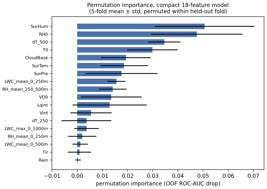
The comparisons above indicate that the compact near-surface model captures most of the available discrimination. To identify the predictors on which this skill rests, we computed permutation feature importance under the same date-grouped protocol: for each of the five folds, each feature column was permuted within the held-out fold (five repeats), and the resulting decrease in out-of-fold ROC-AUC was taken as the importance of that feature. The measure is model-agnostic, requires no surrogate model, and inherits the leakage protections of the evaluation design.
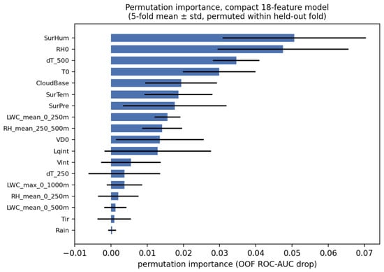
Figure 8 presents the result for the compact 18-feature model. The importance ranking is consistent with the near-surface formation mechanism of coastal sea fog discussed in Section 4.1. The largest contributions come from the two near-surface saturation variables (surface humidity, AUC ; lowest-level relative humidity , 0.048), followed by the 0–500 m temperature difference (0.035), which characterizes the low-level thermal stratification and inversion, and then by the surface and lowest-level temperatures, the retrieved cloud-base height, and the 0–250 m liquid-water content. The precipitation flag, the infrared sky temperature, and the deeper-layer moisture aggregates contribute little.
Figure 8.
Permutation feature importance of the compact 18-feature model (fog state, ): mean ± std over the five date-grouped folds of the out-of-fold ROC-AUC drop when each feature is permuted within the held-out fold (five repeats per feature). Near-surface saturation (surface humidity, ) dominates, followed by the 0–500 m temperature difference (inversion proxy), surface/lowest-level temperature, cloud-base height, and low-level liquid-water content.
These results corroborate two findings of this study. First, the discriminative signal is concentrated in a small number of near-surface thermodynamic and humidity variables, in line with the observation that the compact model suffices and that additional profile depth yields only a marginal gain (Table 7). Second, several of the leading predictors—the low-level stratification, the cloud-base height, and the low-level liquid water—are radiometer retrievals that conventional surface meteorological observations cannot provide, underscoring the central role of the microwave radiometer in the present configuration (Section 4.3).
4. Discussion
4.1. Physical Interpretation and Sensor Division of Labor
The model’s high discriminative power can be explained by the near-surface physical mechanism of sea fog: the occurrence of sea fog is closely linked to near-surface saturation, low-level temperature inversion, and increasing liquid water, and the microwave radiometer is sensitive to changes in near-surface water vapor and integrated liquid water (LWP) and supports long-term continuous observation, so its near-surface thermodynamic/humidity features can robustly support the discrimination of “whether fog exists/will form” [18,20,30]. The millimeter-wave radar, in turn, is irreplaceable for characterizing the vertical structure, thickness, and evolution of the fog layer [14], and may provide complementary microphysical information in the near-saturated hard regime where the radiometer humidity signal saturates (Section 3.4). The two are functionally complementary in principle: the radiometer leans toward “whether fog exists,” while the radar leans toward “the structure and evolution of fog.” In our data this complementarity appears only as a positive but non-significant tendency in the hardest segment; whether it translates into an operational gain remains a hypothesis to be tested with more fog events.
4.2. Benchmarking Against Existing Studies
Placing this work within the lineage of existing sea-fog remote-sensing studies helps to clarify the applicability boundaries of different observation geometries. Scanning millimeter-wave radar has been reported to achieve about 97% accuracy for sea-fog identification [17], with an advantage arising from low-elevation direct planar imaging of the sea-surface fog area and spatial block aggregation; this study adopts a vertically pointing geometry, positioned at “point + vertical structure + multi-lead probability + lead time,” complementing the “area”-oriented work of scanning radar. It should be noted that the metrics of different studies are strongly affected by the task protocol (base rate, splitting scheme); this paper adheres to the operationally realistic base rate and to date-grouped (event-chain-merged) leakage prevention, so that the reported performance is closer to the truly attainable level. Reports that a 94 GHz vehicle-mounted radar is more sensitive to early weak fog [16] likewise suggest that millimeter-wave radar is well suited to characterizing the structure and evolution of fog.
4.3. Transferability and Minimal Sensor Configuration
A natural question is what would be required to deploy this concept at another coastal site. The two profilers were chosen because they are the co-located, continuously operating active/passive pair maintained operationally at the station—the microwave radiometer is a CMA-certified operational instrument—so the data stream is sustainable rather than campaign-based. Importantly, however, the main nowcast model does not require the full (and most expensive) part of this configuration: its 18 inputs are near-surface scalars derived from the radiometer’s lowest retrieval levels and its built-in surface sensors, and the radar contributes only the hard-regime gain that is positive in direction but not statistically confirmed (Section 3.4). The minimal transferable configuration is therefore one operational microwave radiometer plus a visibility sensor: the visibility record supplies the local labels, and the compact model can be retrained and re-calibrated with the same date-grouped protocol on roughly one local fog season of data—no GPU, no radar, and no long archive are needed (the released reuse package retrains the compact model in minutes on a laptop). Whether an even cheaper subset—e.g., standard automatic-weather-station variables without the radiometer’s liquid-water and inversion information—retains sufficient skill is an open question that the permutation-importance analysis (Section 3.5) helps to frame: several of the leading predictors are radiometer-specific retrievals, indicating that the radiometer supplies the essential remote-sensing information in this configuration, with the radar acting as a refinement.
4.4. Limitations and Outlook
Several limitations remain. First, the false alarms of the single-stage alarm mostly fall near the fog/non-fog definitional boundary (genuine low visibility of light/near fog), and a graded visibility sequence and multi-threshold labels could subsequently be introduced to enable graded alarms [31].
Second, the observation geometry is a single vertical column: both instruments profile the atmosphere directly above the station, so the system detects the local precursor state (near-surface saturation, inversion, rising liquid water) but physically cannot see a fog bank forming or advecting 10–20 km upwind. This is precisely why we restrict the lead time to 0–3 h—within this range the local column carries most of the predictive signal, as evidenced by the gentle AUC decay from 0.965 to 0.952 across 0–3 h, whereas extending the lead further would increasingly require the advective context. Coupling the column nowcast with satellite fog products and neighboring coastal stations into a network-level warning is the natural next step, and the calibrated probability output of this study is designed to be one fusible input of such a system.
Third, the feature set contains no sea-surface temperature: the key advection-fog driver—the air–sea temperature difference—is only indirectly represented through the near-surface air temperature and saturation state, because no co-located, quality-controlled SST record with the required continuity was available for the study period. Incorporating a nearby buoy or a gridded SST analysis, and thereby an explicit predictor, is among the most promising single additions for the advection-fog regime and is planned for the network extension.
Fourth, the record covers a single annual cycle at one station: fog events concentrate in spring (39), winter (19), and early summer (13), while autumn contributed none (Table 3). Although discrimination is stable across the represented seasons and months (seasonal AUC 0.94–0.97 with overlapping confidence intervals), a model trained on all seasons jointly necessarily learns compromise weights across potentially season-specific mechanisms (e.g., spring advection versus winter radiation fog); with the present event counts, season-specific models are not yet statistically supportable, and multi-year accumulation is required both to test seasonal specialization and to confirm the hard-regime radar gain, whose direction is positive but whose confidence interval includes zero.
Fifth, the visibility sensor that defines the continuous ground truth also defines the reconstructed event set, so labels and evaluation share one instrument; the manual-record cross-check (41/41 coverage, no false positives) mitigates but does not eliminate this single-sensor circularity, and outages of that sensor directly perturb event boundaries.
Finally, future work could more tightly couple the fog structure/evolution products provided by the radar with the radiometer-dominated probabilistic discrimination, developing a sea-fog monitoring product oriented toward operational running and re-evaluated online as observations accumulate [21,32].
5. Conclusions
Based on the co-located microwave radiometer and millimeter-wave cloud radar at the Xiaoyangshan coastal station and supervised by a continuous, minute-resolution visibility ground truth, we constructed and evaluated a calibrated probabilistic sea-fog nowcasting model. The main conclusions are as follows:
- Under strict, date-grouped, leakage-free evaluation—in which neither input windows nor forecast labels cross fold boundaries—the model attains a ROC-AUC of 0.95–0.96 for the fog state across 0–3 h lead times, and a 3 h onset-AUC of about 0.94, possessing an onset-warning capability several hours in advance.
- After out-of-group isotonic calibration, the model’s output fog probabilities are reliable; the single-stage alarm reaches an event hit rate of 0.84 over the 2026 hold-out period—unchanged when the model, calibrator, and alarm parameters are all strictly frozen on data through 2025 and run forward—with the median first alert about 3.1 h ahead, and the false alarms mostly fall near the fog/non-fog definitional boundary.
- A compact near-surface scalar model already saturates discrimination; the mask-aware radar–radiometer fusion adds only a small, statistically non-significant gain in the near-saturated hard regime, indicating that more independent fog events—rather than a richer model—are the limiting factor. This positive but inconclusive tendency motivates multi-station, multi-season replication.
- The proposed model is lightweight, highly discriminative, and well calibrated, can be locally deployed and re-evaluated as observations accumulate, and provides a practical scheme for short-range coastal sea-fog warning.
Supplementary Materials
The following supporting information can be downloaded at: https://www.mdpi.com/article/10.3390/atmos17080788/s1, Figure S1: Fog-event label completeness drives hold-out performance. The 2026 out-of-time hold-out event hit rate is shown for the manually curated 41-event labels (grey) versus the visibility-reconstructed 71-event labels (blue), under two protocols: a full end-to-end run that trains, tunes, and evaluates the alarm pipeline on each label set (left), and a controlled swap in which the model and all alarm parameters are held fixed and only the label set is changed (right). The reconstructed labels raise the hold-out hit rate from 0.38 to 0.84 end-to-end and from 0.75 to 0.84 under the controlled swap, indicating that label completeness—rather than model choice—drives the improvement. This supports the label-reconstruction procedure described in Section 2.2 of the main text; Figure S2: Event-level bootstrap () 95% confidence intervals for the fog-CSI differences in the near-saturated hard regime (near-surface ): mask-aware fusion minus the compact MLP (), the radar increment defined as fusion minus radiometer-only (), and radar values minus echo-presence (). All three intervals include zero, confirming that the hard-regime radar gain is positive in point estimate but not statistically significant at the present single-station event count. This supports the hard-regime analysis in Section 3.4 of the main text; Figure S3: Sensitivity of the single-stage alarm to the entry threshold, with the other alarm parameters (5 consecutive entry frames, 60-min exit hold, 60-min merge gap) held at their frozen values. (a) Event hit rate versus entry threshold for the 2025 calibration period (blue) and the 2026 hold-out period (orange); the horizontal dotted line marks the ≥0.85 tuning constraint and the vertical dashed line the frozen operating point. (b) False-alarm burden (episodes per month) versus entry threshold. The hold-out hit rate is stable at 0.84 over a wide threshold band around the frozen point, indicating that the reported operating point is not finely tuned; the threshold mainly trades false-alarm burden against calibration-period hit rate. This supports the alarm design of Section 2.4 of the main text; Figure S4: Cross-validation partition-scale ablation: fog-state out-of-fold ROC-AUC of the logistic-regression baseline (calibrated) and the compact MLP when the grouping block is varied from 12 h to 5 days (event-chain merging across block boundaries retained in all cases). Performance is stable across block lengths, indicating that calendar-day grouping already isolates the dominant temporal autocorrelation; larger blocks reduce the number of groups (and thus fold-assignment flexibility) without changing the conclusion. This supports the protocol choice of Section 2.4 of the main text; Figure S5: Seasonal and monthly robustness. (a) Seasonal distribution of the 71 reconstructed fog events (stacked by the 2025 calibration and 2026 hold-out periods); no event occurred in autumn (SON) during the study period. (b) Monthly out-of-fold ROC-AUC of the fog-state discrimination () over the ten months containing both classes. This supports the seasonal analysis of Section 2.2 and the limitations discussion of Section 4.4 of the main text.
Author Contributions
Conceptualization, D.W. and C.L.; methodology, C.L.; software, C.L. and Q.Z.; validation, Q.Z., Y.W. and C.Z.; formal analysis, C.L.; investigation, Y.W. and C.Z.; resources, D.W. and H.C.; data curation, H.C. and Q.Z.; writing—original draft preparation, C.L.; writing—review and editing, D.W. and C.L.; visualization, Q.Z.; supervision, D.W.; project administration, D.W.; funding acquisition, D.W. All authors have read and agreed to the published version of the manuscript.
Funding
This research was funded by the Cooperative Project of the East China Regional Meteorological Science and Technology Collaborative Innovation Fund, grant number QYHZ202303.
Data Availability Statement
The raw observational data used in this study (microwave-radiometer profiles, millimeter-wave cloud-radar profiles, and minute-resolution visibility records) were provided by the Xiaoyangshan National Basic Meteorological Station (Shanghai Meteorological Service) under operational data-use restrictions and cannot be redistributed; they are available from the corresponding author upon reasonable request and subject to permission from the data provider. To ensure reproducibility and reuse, a package—containing the per-sample, leakage-free out-of-fold (OOF) predictions, a derived 18-feature near-surface scalar dataset (from which the compact main model can be retrained), and the code required to recompute all reported performance metrics—is provided in the Supplementary Materials (seafog_atmos_reproducibility.zip) and mirrored at https://github.com/chaoliu-atm/seafog (accessed on 16 July 2026); no raw observations are required to verify the reported results. The vertical profiles are not included, as they constitute near-raw restricted observations.
Acknowledgments
The authors thank the staff of the Xiaoyangshan National Basic Meteorological Station for maintaining the instruments and providing the observational data.
Conflicts of Interest
The authors declare no conflicts of interest.
Abbreviations
The following abbreviations are used in this manuscript:
| MWR | Microwave radiometer |
| MMCR | Millimeter-wave cloud radar |
| LWP | Liquid water path |
| LWC | Liquid water content |
| LDR | Linear depolarization ratio |
| ROC-AUC | Area under the receiver operating characteristic curve |
| AUPRC | Area under the precision–recall curve |
| OOF | Out-of-fold |
| ECE | Expected calibration error |
| POD | Probability of detection |
| FAR | False alarm ratio |
| CSI | Critical success index |
| MLP | Multilayer perceptron |
| TCN | Temporal convolutional network |
| WMO | World Meteorological Organization |
References
- Koračin, D.; Dorman, C.E.; Lewis, J.M.; Hudson, J.G.; Wilcox, E.M.; Torregrosa, A. Marine fog: A review. Atmos. Res. 2014, 143, 142–175. [Google Scholar] [CrossRef] [Scilit]
- Ye, X.Y.; Shen, F.F.; Fei, H.Y.; Sun, Q.L.; Shu, A.Q.; Wan, S.; Chen, H. The study of thermodynamic mechanisms of advection-cooled sea fogs for two cases based on the WRF model. Front. Earth Sci. 2025, 13, 1627881. [Google Scholar] [CrossRef] [Scilit]
- Zhang, S.P.; Xie, S.P.; Liu, Q.Y.; Yang, Y.Q.; Wang, X.G.; Ren, Z.P. Seasonal Variations of Yellow Sea Fog: Observations and Mechanisms. J. Clim. 2009, 22, 6758–6772. [Google Scholar] [CrossRef] [Scilit]
- Shi, X.; Yi, L.; Zhang, S.; Shi, X.; Liu, Y.; Liu, Y.; Wang, X.; Jiang, Y. Microphysical Characteristics of a Sea Fog Event with Precipitation Along the West Coast of the Yellow Sea in Summer. Atmosphere 2025, 16, 308. [Google Scholar] [CrossRef] [Scilit]
- Koračin, D. Modeling and Forecasting Marine Fog. In Marine Fog: Challenges and Advancements in Observations, Modeling, and Forecasting; Springer International Publishing: Cham, Switzerland, 2017; pp. 425–475. [Google Scholar] [CrossRef] [Scilit]
- Zhang, L.; Xu, M.; Qiu, X.; Zhang, D.; Liao, R.; Fang, X.; Wu, B.; Meng, F. Analysis of Spatio-Temporal Characteristics of Visibility in the Yellow and Bohai Seas Based on Observational Data. Atmosphere 2023, 14, 1101. [Google Scholar] [CrossRef] [Scilit]
- Bari, D.; Lasri, N.; Souri, R.; Lguensat, R. Machine Learning for Fog-and-Low-Stratus Nowcasting from Meteosat SEVIRI Satellite Images. Atmosphere 2023, 14, 953. [Google Scholar] [CrossRef] [Scilit]
- Xu, M.; Chen, K.; Guo, H.; Huang, Y.; Wu, M.; Shi, Z.; Zhang, C.; Guo, J. MFogHub: Bridging Multi-Regional and Multi-Satellite Data for Global Marine Fog Detection and Forecasting. arXiv 2025, arXiv:2505.10281. [Google Scholar] [CrossRef] [Scilit]
- Mahdavi, S.; Amani, M.; Bullock, T.; Beale, S. Enhanced oceanic fog nowcasting through satellite-based recurrent neural networks. Big Earth Data 2024, 9, 505–524. [Google Scholar] [CrossRef] [Scilit]
- Kim, Y.H.; Moon, S.H.; Yoon, Y. Detection of Precipitation and Fog Using Machine Learning on Backscatter Data from Lidar Ceilometer. Appl. Sci. 2020, 10, 6452. [Google Scholar] [CrossRef] [Scilit]
- Aguirre, R.; Toledo, F.; Rodríguez, R.; Rondanelli, R.; Reyes, N.; Díaz, M. Low-Cost Ka-Band Cloud Radar System for Distributed Measurements within the Atmospheric Boundary Layer. Remote Sens. 2020, 12, 3965. [Google Scholar] [CrossRef] [Scilit]
- Lin, H.; Wang, J.; Ge, J. A Cloud Detection Method for Vertically Pointing Millimeter-Wavelength Cloud Radar. Sensors 2023, 23, 8891. [Google Scholar] [CrossRef] [Scilit] [PubMed]
- Liu, L.; Ruan, Z.; Zheng, J.; Gao, W. Comparing and Merging Observation Data from Ka-Band Cloud Radar, C-Band Frequency-Modulated Continuous Wave Radar and Ceilometer Systems. Remote Sens. 2017, 9, 1282. [Google Scholar] [CrossRef] [Scilit]
- Boers, R.; Baltink, H.K.; Hemink, H.J.; Bosveld, F.C.; Moerman, M. Ground-Based Observations and Modeling of the Visibility and Radar Reflectivity in a Radiation Fog Layer. J. Atmos. Ocean. Technol. 2013, 30, 288–300. [Google Scholar] [CrossRef] [Scilit]
- Bell, A.; Martinet, P.; Caumont, O.; Vié, B.; Delanoë, J.; Dupont, J.C.; Borderies, M. W-band radar observations for fog forecast improvement: An analysis of model and forward operator errors. Atmos. Meas. Tech. 2021, 14, 4929–4946. [Google Scholar] [CrossRef] [Scilit]
- Shi, R.; Li, C.; Lei, Y.; Guan, Y.; Zhang, Y. Sea Fog Microphysics and Visibility Retrieval Using a 94-GHz Millimeter-Wave Radar on an Uncrewed Surface Vehicle. IEEE Trans. Geosci. Remote Sens. 2026, 64, 5100310. [Google Scholar] [CrossRef] [Scilit]
- Li, T.; Qiu, J.; Xue, J. Sea Fog Recognition near Coastline Using Millimeter-Wave Radar Based on Machine Learning. Atmosphere 2024, 15, 1031. [Google Scholar] [CrossRef] [Scilit]
- Martinet, P.; Unger, V.; Burnet, F.; Georgis, J.F.; Hervo, M.; Huet, T.; Löhnert, U.; Miller, E.; Orlandi, E.; Price, J.; et al. A dataset of temperature, humidity, and liquid water path retrievals from a network of ground-based microwave radiometers dedicated to fog investigation. Bull. Atmos. Sci. Technol. 2022, 3, 6. [Google Scholar] [CrossRef] [Scilit]
- Guy, H.; Turner, D.D.; Walden, V.P.; Brooks, I.M.; Neely, R.R. Passive ground-based remote sensing of radiation fog. Atmos. Meas. Tech. 2022, 15, 5095–5115. [Google Scholar] [CrossRef] [Scilit]
- Chan, P.W.; Cheung, P.; Ho, C.K.; Amaireh, A.; Zhang, Y.; Leung, Y.Y. Microwave Radiometer Observations of Cloud Liquid Water Content in Hong Kong: Fog, Spring-Time Clouds, Rainstorms, and Typhoon. Appl. Sci. 2025, 15, 11478. [Google Scholar] [CrossRef] [Scilit]
- Salcedo-Sanz, S.; Guijo-Rubio, D.; Pérez-Aracil, J.; Peláez-Rodríguez, C.; Gomez-Orellana, A.M.; Gutiérrez-Peña, P.A. Artificial Intelligence-Based Methods and Algorithms in Fog and Atmospheric Low-Visibility Forecasting. Atmosphere 2025, 16, 1073. [Google Scholar] [CrossRef] [Scilit]
- TK001 Ground-Based Microwave Radiometer: Product Technical Documentation; Manufacturer’s Technical Datasheet; Shanghai Leitang Technology Co., Ltd.: Shanghai, China, 2026.
- Liljegren, J.C.; Clothiaux, E.E.; Mace, G.G.; Kato, S.; Dong, X. A new retrieval for cloud liquid water path using a ground-based microwave radiometer and measurements of cloud temperature. J. Geophys. Res. Atmos. 2001, 106, 14485–14500. [Google Scholar] [CrossRef] [Scilit]
- Tang, W.; Long, G.; Liu, L.; Zhou, T.; Blumenstein, M.; Jiang, J. Omni-Scale CNNs: A simple and effective kernel size configuration for time series classification. arXiv 2020, arXiv:2002.10061. [Google Scholar] [CrossRef] [Scilit]
- Bai, S.; Kolter, J.Z.; Koltun, V. An Empirical Evaluation of Generic Convolutional and Recurrent Networks for Sequence Modeling. arXiv 2018, arXiv:1803.01271. [Google Scholar] [CrossRef] [Scilit]
- Cui, Y.; Jia, M.; Lin, T.Y.; Song, Y.; Belongie, S. Class-Balanced Loss Based on Effective Number of Samples. In Proceedings of the 2019 IEEE/CVF Conference on Computer Vision and Pattern Recognition (CVPR); IEEE: Piscataway, NJ, USA, 2019; pp. 9260–9269. [Google Scholar] [CrossRef] [Scilit]
- Zadrozny, B.; Elkan, C. Transforming classifier scores into accurate multiclass probability estimates. In Proceedings of the Eighth ACM SIGKDD International Conference on Knowledge Discovery and Data Mining; Association for Computing Machinery: New York, NY, USA, 2002; pp. 694–699. [Google Scholar] [CrossRef] [Scilit]
- Niculescu-Mizil, A.; Caruana, R. Predicting good probabilities with supervised learning. In Proceedings of the 22nd International Conference on Machine Learning (ICML); Association for Computing Machinery: New York, NY, USA, 2005; pp. 625–632. [Google Scholar] [CrossRef] [Scilit]
- Brier, G.W. Verification of Forecasts Expressed in Terms of Probability. Mon. Weather Rev. 1950, 78, 1–3. [Google Scholar] [CrossRef] [Scilit]
- Temimi, M.; Fonseca, R.M.; Nelli, N.R.; Valappil, V.K.; Weston, M.J.; Thota, M.S.; Wehbe, Y.; Yousef, L. On the analysis of ground-based microwave radiometer data during fog conditions. Atmos. Res. 2020, 231, 104652. [Google Scholar] [CrossRef] [Scilit]
- Song, J.I.; Yum, S.S.; Gultepe, I.; Chang, K.H.; Kim, B.G. Development of a new visibility parameterization based on the measurement of fog microphysics at a mountain site in Korea. Atmos. Res. 2019, 229, 115–126. [Google Scholar] [CrossRef] [Scilit]
- Martinet, P.; Cimini, D.; Burnet, F.; Ménétrier, B.; Michel, Y.; Unger, V. Improvement of numerical weather prediction model analysis during fog conditions through the assimilation of ground-based microwave radiometer observations: A 1D-Var study. Atmos. Meas. Tech. 2020, 13, 6593–6611. [Google Scholar] [CrossRef] [Scilit]

Disclaimer/Publisher’s Note: The statements, opinions and data contained in all publications are solely those of the individual author(s) and contributor(s) and not of MDPI and/or the editor(s). MDPI and/or the editor(s) disclaim responsibility for any injury to people or property resulting from any ideas, methods, instructions or products referred to in the content. |
© 2026 by the authors. Licensee MDPI, Basel, Switzerland. This article is an open access article distributed under the terms and conditions of the Creative Commons Attribution (CC BY) license.