


Abstract
This study presents a multivariate spatio-temporal clustering framework to characterise joint wind–wave regimes across European seas using the fifth-generation atmospheric reanalysis produced by the European Centre for Medium-Range Weather Forecasts (ERA5; 1979–2014). Seasonal and annual statistics of significant wave height, mean wave period, wind speed, and wave/wind direction were computed at 0.5° resolution. Principal component analysis was used to reduce dimensionality, retaining 30 components that captured 99% of the variance. K-means clustering was then used to identify nine coherent dynamical regimes with persistent spatio-temporal signatures. These regimes were grouped into open-ocean, transitional, and enclosed/semi-enclosed categories based on internal variability, directional spread, and geographic exposure. Open-Atlantic regimes are found to be energy-rich, exhibiting clear December–February maxima in significant wave height (), mean wave period (), and 10 m wind speed (); enclosed and semi-enclosed basins show lower amplitudes and reduced variability, while transitional shelves and the southern Mediterranean display intermediate conditions, characterised by moderate levels and seasonal rotation of wave and wind directions, reflecting a mixed influence of locally generated seas and remotely forced swell. Dispersion analysis highlights a clear Atlantic–Mediterranean partition, with transitional shelves forming a dynamical bridge between open-ocean and enclosed basins. Teleconnection analysis shows that the North Atlantic Oscillation and Arctic Oscillation dominate Atlantic regimes, while the Scandinavia, East Atlantic, and Polar/Eurasia patterns modulate variability and directional persistence in transitional and enclosed seas. The classification defines a climatological framework of European wind–wave conditions and establishes a practical basis for renewable energy assessment, engineering design, and long-term change analysis, with methods transferable to other basins.
1. Introduction
Near-surface wind–wave conditions are key components of the coupled ocean–atmosphere system, shaping coastal erosion, sediment transport, and energy transfer and affecting offshore infrastructure and marine ecosystems [1,2,3]. At larger scales, winds and waves contribute to ocean mixing, nutrient upwelling, and carbon cycling [2,4,5]. Wind–wave variability arises from atmospheric circulation, storm activity, and local geography [6,7]. Understanding seasonal and interannual variability improves knowledge of regional climate, supports coastal and offshore planning, and places observed trends in a broader context. With changing storm patterns and more frequent extremes, it is increasingly important to identify spatial patterns and long-term changes in wind–wave conditions [8,9].
Despite their physical connection, wind and wave conditions have often been assessed separately. Previous studies have primarily examined individual parameters, including significant wave height [1,8], wave period [4], and wind speed [9,10]. Across European seas, research has documented basin-specific trends and variability [7,8,11,12], investigated wave energy and coastal-protection applications [13,14], and examined storm impacts and regional atmospheric and oceanic controls [15,16,17,18]. Recent studies have examined the Adriatic wind–wave climate using bias-corrected forcing from the fifth-generation atmospheric reanalysis produced by the European Centre for Medium-Range Weather Forecasts (ERA5) [19], long-term wave power trends across the Mediterranean [20], and the seasonal, interannual, and North Atlantic Oscillation (NAO)-related variability of wave resources in the Irish Sea [21]. Joint wind–wave resource assessments have also been conducted for European offshore sites under Coupled Model Intercomparison Project Phase 6 (CMIP6) projections [22] and along mainland Portugal [23]. Wind-only model assessments nevertheless remain common. For example, Çalışır et al. [24] evaluated 22 CMIP6 models for wind-resource assessment and showed that model performance varies across regions and wind regimes, with EC-Earth3 performing well over the Mediterranean. Although recent studies increasingly consider both wind and wave resources, they generally focus on individual basins, selected energy sites, resource co-location, or projected changes. They do not provide a European-scale classification based on the long-term joint variability of multiple wind and wave parameters.
Several methodological approaches have attempted to organise wind–wave variability. Earlier wave-clustering methods were used to identify dominant wave regimes and classify coastal environments [25], while synoptic-climatology approaches classified atmospheric circulation patterns and examined their influence on wave conditions [26]. More recent studies have extended these methods. Odériz et al. [27] developed a multivariate dynamic classification of global wave climates and related their variability to atmospheric circulation. Lobeto et al. [28] used clustering to identify homogeneous regions of projected change in directional wave spectra, while Goharnejad et al. [29] applied Spatial Neural Gas clustering to seasonal extreme-wave conditions in the Northwest Atlantic. Zhao et al. [30] incorporated wave clustering into a weather-type statistical downscaling model. Gridded trend analyses and regional averaging provide additional information on long-term changes, but can mask local interactions and coherent spatial structures [31]. Studies of wind–wave dependence have also demonstrated the importance of considering the variables jointly for understanding atmospheric forcing, ocean response, and marine energy conditions [32,33,34]. However, recent classification methods remain centred mainly on wave variables, directional spectra, extreme conditions, or statistical downscaling. They do not classify fixed grid cells across the European domain according to the combined seasonal and interannual behaviour of wind speed, wave height, wave period, and wind and wave directions.
Despite these advances, a unified framework for classifying European marine regions according to their long-term wind–wave co-variability is still lacking. In particular, existing approaches do not simultaneously integrate multiple wind and wave parameters, represent their seasonal and interannual variability, and identify spatially coherent regions with comparable behaviour. It therefore remains unclear whether distinct wind–wave regimes can be identified across contrasting European seas, how internally consistent these regimes are, and how their behaviour varies across seasons and years.
To address this gap, this study develops a data-driven framework for identifying spatially coherent regimes from the joint, multi-decadal variability of wind and wave conditions. Using ERA5 reanalysis data [35], we combine seasonal and annual statistics of key wind and wave parameters to represent both the mean conditions and their variability at each grid cell. Principal component analysis (PCA) is used to summarise the multivariate information, after which grid cells, rather than individual years, are grouped using k-means clustering according to the similarity of their multi-decadal wind–wave behaviour. The study specifically aims to: (i) identify coherent wind–wave climate regimes across the European seas; (ii) quantify their seasonal and interannual variability; and (iii) examine how the temporal variability of the identified regimes relates to large-scale climate modes. By treating wind and wave conditions as an interconnected system, the framework provides a consistent basis for comparing marine climate variability across regions, seasons, and decades and can be transferred to other ocean basins.
The remainder of this paper is organised as follows. Section 2 describes the ERA5 dataset, preprocessing, dimensionality reduction, and clustering methodology. Section 3 presents the identified wind–wave regimes, their temporal variability, and their relationships with large-scale climate modes. Finally, Section 4 summarises the main findings, discusses the limitations, and outlines directions for future research.
2. Data and Methodology
The approach involves five main steps: (1) extracting wind and wave parameters from ERA5 (1979–2014) and deriving 10 m wind speed and direction from the wind components (see Section 2.2); (2) aggregating seasonal (December–February (DJF), March–May (MAM), June–August (JJA), and September–November (SON), with December assigned to the following DJF year) and annual statistics, using the sample standard deviation and circular averaging/dispersion for directional variables (see Section 2.2.1); (3) standardising all variables and applying principal component analysis (PCA) to reduce dimensionality (see Section 2.3); (4) performing k-means clustering () to identify spatial regimes (see Section 2.4); and (5) evaluating intra- and inter-cluster variability and linking clusters and variables to large-scale climate oscillations via (circular) Spearman correlations (see Section 2.6). Figure 1 summarises the workflow, including preprocessing and clustering. Subsequent sections describe each component in detail.
Figure 1.
Overview of the methodology workflow. Fifth-generation atmospheric reanalysis fields from the European Centre for Medium-Range Weather Forecasts (ERA5; 1979–2014) are aggregated to seasonal and annual statistics (using circular statistics for directions). Fifty features (5 variables × 5 periods × 2 statistics) are standardised and reduced via principal component analysis (PCA) for each grid-cell–year; the first 30 principal component (PC) scores (explaining ∼99% of variance) are concatenated across 36 years and clustered with k-means (). Outputs include intra-/inter-cluster variability and correlations with large-scale teleconnection indices (Spearman).
2.1. Data Description
We analyse the ERA5 reanalysis from the European Centre for Medium-Range Weather Forecasts (ECMWF) for 1979–2014, which provides a continuous, homogenised reconstruction of near-surface wind and wave conditions based on the Integrated Forecast System with assimilated in situ and satellite observations. The considered variables include significant wave height (, m), mean wave period (, s), mean wave direction (, °), 10 m wind speed (, m s−1), and 10 m wind direction (, °). Wind quantities are derived from the 10 m zonal and meridional components (, ). All variables were derived from hourly ERA5 fields, regridded to , and aggregated to seasonal (DJF, MAM, JJA, SON) and annual statistics. For each variable, we compute the mean and standard deviation; for wave and wind directions, circular means and circular standard deviations are used. The analysis domain spans W– E and N– N (Figure 2), covering the dynamically active wind–wave systems of the European seas [36].
Figure 2.
ERA5 wind–wave regimes (), 1979–2014. Nine spatial regimes obtained by k-means clustering of 1080-dimensional descriptors formed by concatenating 30 PC scores (explaining ≈99% of variance) across 36 years. The scores were derived from seasonal and annual statistics of , , , , and . Colours indicate cluster membership; labels denote abbreviations (NWAC, BSC, SMC, WMIC, EAC, NEC, EMC, SCES, WENS).
The analysis period was deliberately restricted to 1979–2014 to provide a historical reference consistent with the nominal CMIP6 historical experiment, which ends in 2014 [37]. This common period was selected to support the subsequent transfer of the ERA5-derived principal component and clustering framework to EC-Earth3 Scenario Model Intercomparison Project (ScenarioMIP) and High Resolution Model Intercomparison Project (HighResMIP) simulations under directly comparable historical forcing. The objective of the present study is to develop and test the wind–wave classification methodology over a consistent multi-decadal reference period, rather than to provide an assessment of changes extending to present-day conditions. The framework itself is not restricted to this period and can be applied to more recent or future datasets.
ERA5 was selected because it provides temporally continuous and internally consistent wind and wave variables over the full European domain and study period. Nevertheless, ERA5 is a model-based reconstruction rather than a spatially complete observational record. Its wind and wave fields are affected by the assimilation system, model physics, spatial resolution, and the representation of coastlines and bathymetry. Previous evaluations have reported spatially varying errors in coastal settings, including underestimation of extreme significant wave heights and high-percentile wind speeds in some regions [38,39]. Recent assessments further show that reanalysis-related uncertainties depend on the region and application. Giudici et al. [40] found that simulated Baltic wave statistics varied with the modelled wind dataset used to force the wave hindcast, while Gandoin and Garza [41] documented an underestimation of strong offshore wind speeds in ERA5. Because an independent reanalysis product is not included here, the resulting principal component structure, cluster membership, and regime boundaries should be interpreted as ERA5-derived rather than dataset-independent geographical boundaries.
Water depth affects wave propagation, and the distinction between deep- and shallow-water waves depends on the relative depth (h/L), where (h) is water depth and (L) is wavelength [32]. Bathymetry was not included as a separate clustering variable. However, ERA5 accounts for model bathymetry and depth-dependent wave propagation, so these effects are indirectly represented in (), (), and wave direction [32,35]. The open-ocean, transitional, and enclosed/semi-enclosed categories should therefore be understood as broad regional settings rather than formal deep- or shallow-water classes.
2.2. Data Preprocessing
2.2.1. Seasonal and Annual Aggregation
The dataset was grouped into four standard climatological seasons—DJF, MAM, JJA, and SON—together with annual values. For each variable, we computed seasonal and annual means and standard deviations. Directional parameters ( and ) were processed using circular mean and circular standard deviation to account for angular wrap-around.
2.2.2. Directional Variables ( and )
Directional quantities were treated using circular statistics to avoid discontinuities at the boundary. For any directional data , the mean direction was obtained from a vector (trigonometric) average:
Circular standard deviation was computed from the mean resultant length following standard circular statistics definitions [42].
The mean resultant length R is defined as
For waves, corresponds to the ERA5 mean wave direction [35].
For winds, instantaneous direction was first derived from the 10 m components as
and the same circular averaging was applied to obtain period means.
2.2.3. Wind Speed Calculation
Wind speed at 10 m was computed from the zonal and meridional components as
Wind variables were combined with wave parameters to form a unified dataset for the spatio-temporal analysis.
2.3. Principal Component Analysis (PCA)
PCA was used to compress the 50-dimensional feature vector (five variables × five periods × mean/standard deviation) at each grid–cell–year into a smaller set of orthogonal modes that capture the dominant covariance patterns in the wind–wave system [43]. This facilitates both noise reduction and efficient downstream clustering of spatio-temporal regimes.
- Standardisation
Let denote the feature vector () for grid cell g and year t. Each variable was standardised across all grid cells and years
where are the sample mean and (sample) standard deviation of feature j. Directional features (mean wave direction and mean wind direction) were entered as circular means (in degrees) and circular standard deviations (degrees) as computed in Section 2.2.2. After circular aggregation, these quantities were treated as scalar variables and standardised in the same way as the other variables.
- PCA Estimation
Principal Component Analysis (PCA) was applied to the standardised data matrix , where N denotes the number of grid-cell–year samples. PCA was implemented using a standard singular value decomposition to obtain orthogonal modes that capture the dominant covariance structure of the wind–wave variables [43].
- Component Retention and Representation
A scree test and the cumulative variance curve indicated that the first components account for approximately of the total variance. We therefore retained 30 principal components (PCs) and discarded the remainder. For each grid cell g and year t, let denote the retained PC score vector. To preserve the interannual structure in the subsequent clustering, the 36 yearly score vectors were concatenated into a single feature vector per grid cell, as described in Section 2.4.
2.4. Clustering Analysis
The classification uses a multivariate feature set composed of the seasonal and annual mean and standard deviation of five variables: significant wave height (), mean wave period (), wind speed (), wave direction (), and wind direction (). These features form the input to the PCA.
We used k-means to identify spatial wind–wave regimes from the PCA representation of ERA5. The method is suitable for this application because it handles large datasets efficiently, performs well in PCA-transformed spaces, and produces centroid-based groups that can be interpreted as representative multivariate conditions [43,44,45]. Compared with density- or graph-based approaches, which may be sensitive to parameter settings or irregular cluster geometry, k-means provides a consistent and computationally straightforward partitioning of the data [46]. All clustering was carried out using the full-batch k-means++ initialisation with multiple restarts to ensure stable solutions.
Uncertainty in the classification arises from both methodological choices and the input dataset. To examine sensitivity to feature selection, we repeated the analysis using alternative feature sets. A qualitative comparison showed that using a single variable, such as , produced broad spatial patterns similar to those obtained using the complete multivariate feature set, although differences occurred along local cluster boundaries and in transitional regions. This suggests that the large-scale organisation is relatively insensitive to feature selection, whereas finer-scale regime boundaries are more sensitive to the variables included. The results may also depend on the selected temporal aggregation and spatial-domain definition, which were held fixed in the present analysis.
This feature set comparison assesses methodological sensitivity but does not quantify uncertainty associated with the use of ERA5. Systematic or spatially varying errors in wind speed and direction, wave height, period, or direction can affect the covariance structure, principal component scores, cluster centroids, and resulting regime boundaries. Aggregation to seasonal and annual statistics may reduce the influence of short-term random errors, while concatenating the PC scores across 1979–2014 ensures that the classification represents the complete multidecadal evolution at each grid cell. However, neither step removes persistent reanalysis biases. The degree to which the identified regimes would remain unchanged under an alternative reanalysis therefore remains unresolved, particularly in coastal, transitional, and semi-enclosed regions where local processes may be less well represented.
- Clustering Input (Spatio-Temporal Vectors)
Let denote the retained PC score vector (Section 2.3) for grid cell g in year , where each score vector already represents seasonal and annual statistics for that year. To embed interannual evolution in each location’s descriptor, we concatenated PC score vectors across all years into a single vector
The set (one 1080-dimensional vector per grid cell) formed the input to k-means.
- Objective Function and Distance
Given k clusters with centroids in , the within-cluster sum of squares (inertia) minimised by k-means is
i.e., squared Euclidean distance in the concatenated PC-score space.
- Cluster Validation and Selection
We evaluated k from 2 to 20 using (i) the elbow method (inertia vs. k) and (ii) the silhouette coefficient
where a is the mean intra-cluster distance and b is the mean distance to the nearest neighbouring cluster. Both diagnostics indicated a clear elbow and stable behaviour at , which we adopted.
For ERA5 (concatenated 30-PC score space; 1080 dimensions; ), the overall silhouette was . Mean silhouettes by cluster were: 0 (0.334), 1 (0.131), 2 (0.416), 3 (0.258), 4 (0.364), 5 (0.166), 6 (0.219), 7 (0.126), 8 (0.273). Clusters 2 and 4 were the most separated, whereas 1 and 7 were comparatively less distinct. Sensitivity checks varying k (6–12), the number of retained PCs (20–40), and random seeds yielded consistent spatial boundaries and labels, supporting robustness.
2.5. Cluster Variability Analysis
We quantified within and between cluster variability directly in the principal component (PC) space used for clustering. This keeps the metric consistent with the k-means objective (squared Euclidean distance) and avoids mixing physical units. Let denote a grid cell’s concatenated PC score vector with (Section 2.4).
2.5.1. Centroids in PC Space
For cluster k with member set containing grid cells, the centroid is
2.5.2. Intra–Cluster Variability
For each member , we measured its deviation from the assigned centroid using the Euclidean () distance
The distribution of was summarised by , mean, standard deviation, and quartiles to characterise each cluster’s internal spread (smaller values indicate more homogeneous regimes).
2.5.3. Inter–Cluster Variability
Between clusters i and j we computed the centroid-to-centroid distance
forming a symmetric distance matrix that measures separation among regimes.
Distances are unitless (PC scores from standardised features). Using Euclidean metrics in PC space aligns with the k-means criterion and provides a consistent basis for comparing intra- vs. inter-cluster structure.
2.6. Climate Oscillation Indices
To examine the influence of large-scale climate patterns on regional wind and wave conditions, a set of climate indices was incorporated into the analysis, as summarised in Table 1. The indices are the North Atlantic Oscillation (NAO), Scandinavia pattern (SCAND), East Atlantic pattern (EA), East Atlantic/Western Russia pattern (EAWR), Arctic Oscillation (AO), Pacific/North American pattern (PNA), West Pacific pattern (WP), and Polar/Eurasia pattern (POLEUR). These indices capture key atmospheric and oceanic modes that can affect surface variability through teleconnections. The selection was based on their relevance to both European and global climate systems.
Table 1.
Climate oscillations and their definitions. Abbreviations: AO, Arctic Oscillation; EA, East Atlantic; EAWR, East Atlantic/Western Russia; NAO, North Atlantic Oscillation; PNA, Pacific/North American; POLEUR, Polar/Eurasia; SCAND, Scandinavia; WP, West Pacific.
These indices were obtained from the National Centers for Environmental Prediction (NCEP). Seasonal (DJF, MAM, JJA, SON) and annual averages were used to match the temporal resolution of the wave and wind dataset.
Correlation Metric (Spearman)
Associations were quantified using Spearman’s rank correlation coefficient () for all variables. A rank-based measure is appropriate here because the series may be non-Gaussian, skewed, or heteroscedastic, sample sizes per period are modest (), and relationships may be monotonic but not strictly linear. Spearman’s correlation is robust to outliers and corresponds to the Pearson correlation computed on ranked data.
Two-tailed p-values were obtained using the large-sample t approximation, and correlations with were considered statistically significant. For each grid cell, climate index, variable, and temporal period, both the correlation coefficient and its associated p-value were computed. Only statistically significant correlations were retained for analysis and subsequent spatial mapping. For visualisation, an additional magnitude threshold () was applied to emphasise stronger associations and improve interpretability.
For angular variables (wave direction and wind direction ), circularity was addressed by projecting directions onto their sine and cosine components. Spearman correlations were computed separately for each projection with the teleconnection index, and the component yielding the larger absolute correlation was retained along with its associated p-value. This approach preserves the robustness of rank-based correlation while accounting for the wrap-around inherent to directional data.
3. Results and Discussion
3.1. Cluster Identification
Clustering of 1080-dimensional descriptors formed by concatenating the first 30 PC scores across 36 years (the PCs captured ≈99% of variance) produced nine spatially coherent wind–wave regimes across 1979–2014 (Figure 2). The resulting clusters are Northern European Continental (NEC), Eastern Mediterranean (EMC), Southern Mediterranean (SMC), Southern and Coastal European Seas (SCES), Eastern Atlantic (EAC), Northwestern Atlantic (NWAC), Western European and Northern Sea (WENS), Western Mediterranean and Iberian (WMIC), and the Baltic Sea (BSC). Consistent with their setting, these regimes were grouped into open-ocean, transitional, and enclosed/semi-enclosed categories (Table 2).
Table 2.
Regional clusters () and qualitative geographic classification.
Although plotted here spatially (e.g., on a map), the partition is intrinsically spatio-temporal. Each grid cell is represented by a time-integrated descriptor that embeds its seasonal and annual behaviour over 1979–2014 (Section 2.4). Thus, the regimes are not instantaneous snapshots; they reflect persistent, multi-decadal structure in joint wind–wave variability.
The resulting geography exhibits coherent “fingerprints’’ shaped by consistent multivariate signals rather than by coastline geometry or masking. Open-ocean domains (e.g., NEC, EAC) are clearly separated from enclosed basins (e.g., BSC, EMC), while transitional interfaces such as WMIC and WENS emerge where gradients in wind–wave climate are strongest (Figure 2). These intermediate regions arise from the data-driven signatures in principal component space, not from spatial proximity alone.
Importantly, the method respects real-world geophysical distinctions without enforcing predefined boundaries. It captures gradients across the domain, enabling a physically interpretable classification. This structure establishes a stable baseline for tracking seasonal and interannual dynamics within each regime and supports further analysis of variability and potential drivers in the sections that follow.
3.2. Atlantic–Mediterranean Cluster Separation
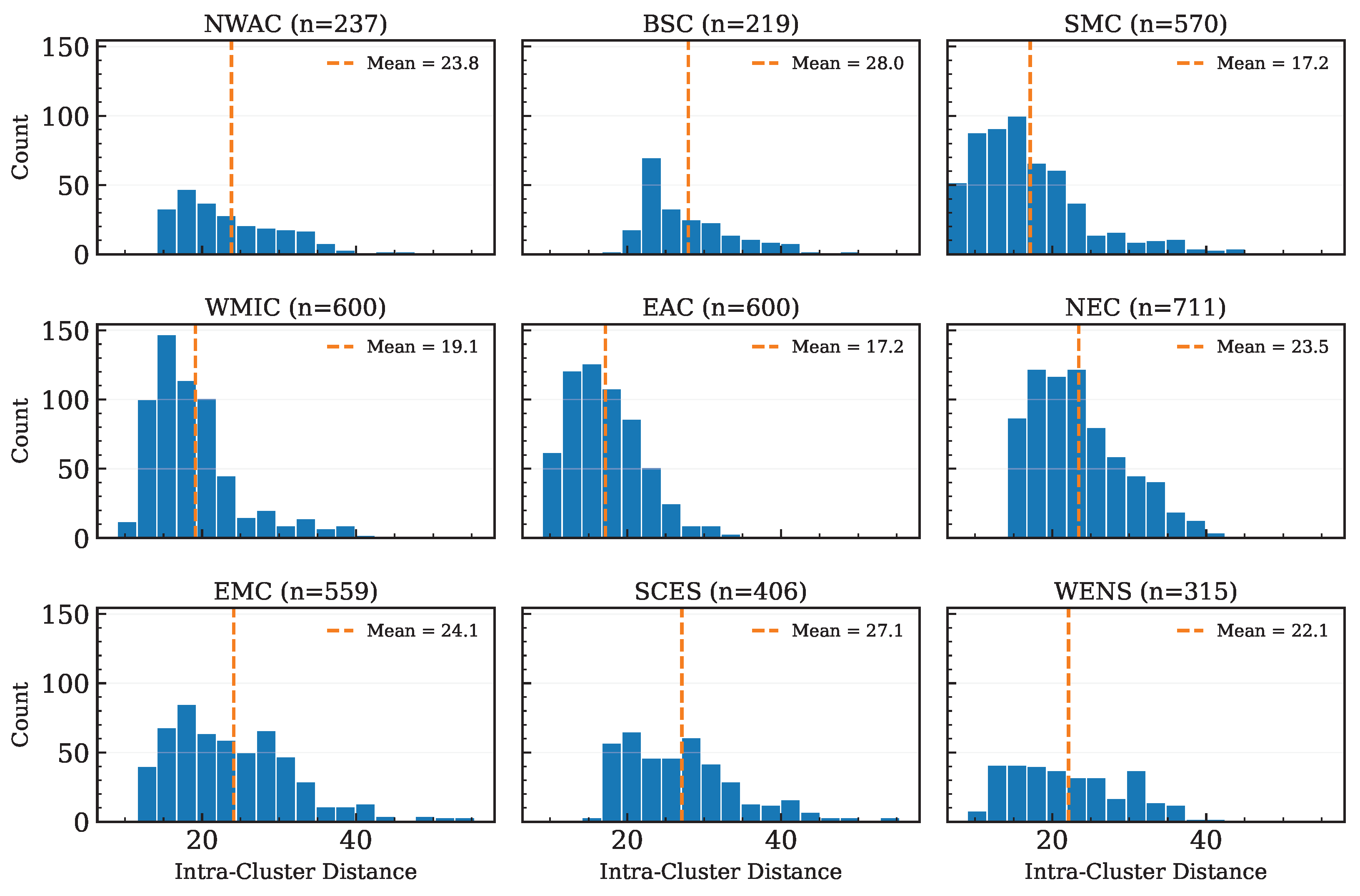
Intra-cluster variability was quantified as the Euclidean distance from each grid cell to its cluster centroid in the 1080-dimensional concatenated PC-score space. Figure 3 summarises the statistical spread of distances across regimes, while the full distance distributions are provided in Appendix A for completeness. The most compact regimes are SMC and EAC, with low cluster-mean distances (≈17–18). By contrast, EMC (≈24.1), SCES (≈27.1), and BSC (≈28.0) display broad dispersion, with BSC showing the highest mean distance overall. NEC, NWAC, WENS, and WMIC fall into the intermediate range (≈19–24). Within this group, WMIC lies toward the compact end, while NEC, NWAC, and WENS exhibit greater spread.
Figure 3.
Intra-cluster variability by regime (ERA5, ). Boxplots of Euclidean distances from each grid cell to its cluster centroid in the 1080-dimensional concatenated PC-score space (dimensionless); boxes show medians and interquartile ranges (IQRs), whiskers denote , and points indicate outliers.
The compactness of EAC reflects swell-dominated conditions and long, uniform fetches across the Atlantic, while SMC indicates relatively coherent forcing in the southern Mediterranean. In contrast, EMC, SCES, and BSC exhibit broad variability consistent with semi-enclosed geometry, complex coastlines, and heterogeneous local winds. The particularly high dispersion in BSC is further linked to shallow depth, limited fetch, strong coastal gradients, and seasonal ice effects. Intermediate regimes reflect mixed forcing: WMIC remains comparatively cohesive, while NEC, NWAC, and WENS show higher variability, with NWAC especially influenced by storm-track activity in the North Atlantic.
Inter-cluster distances (Figure 4) confirm separation between regimes. The largest centroid distances occur between EAC–WMIC (≈80.9), EAC–WENS (≈72.9), and EAC–EMC (≈70.3), marking large differences in multivariate wind–wave statistics between the open-Atlantic and transitional or eastern Mediterranean regimes. The smallest distance is between WMIC–WENS (≈25.0), reflecting their shared transitional character. Enclosed and semi-enclosed basins are not uniformly similar: EMC is distant from both SMC and SCES (≈64.6 and ≈60.8, respectively), while BSC occupies a mid-range position.
Figure 4.
Inter-cluster separation (centroid distances; ERA5, ). Symmetric matrix of Euclidean distances between cluster centroids computed in the 1080-dimensional concatenated PC-score space (dimensionless). Larger values indicate stronger dissimilarity in multivariate wind–wave statistics; diagonal entries are zero.
These patterns are consistent with basin-scale forcing. Transitional clusters (WMIC, WENS) are statistically close to EMC but remain well separated from EAC, forming bridges between open-ocean and enclosed basins. The large Atlantic–Mediterranean separations reflect distinct circulation regimes, while the intermediate position of BSC highlights the heterogeneous character of semi-enclosed seas. Boxplots and histograms show that WMIC and WENS occupy intermediate dispersion ranges broader than EAC but narrower than EMC and SCES, consistent with their dual exposure to Atlantic and Mediterranean processes. Among transitional clusters, SMC is comparatively compact.
Together, these results indicate a balanced and robust nine-cluster solution. Compact regimes (EAC and SMC) provide consistent baselines for region-specific forecasting of seasonal to interannual conditions. Large inter-basin distances across the Atlantic–Mediterranean divide (EAC–WMIC = 80.9; EAC–WENS = 72.9; EAC–EMC = 70.3) delineate contrasts in wind–wave regimes, informing energy planning where resource potential and design conditions differ substantially. Transitional regimes (e.g., WMIC–WENS = 25.0) identify zones where open-ocean and enclosed-basin processes interact, which is relevant for evaluating combined forcing in siting and operational strategies. Enclosed regimes with broad dispersion (e.g., EMC, SCES, BSC) define areas where local wind and boundary effects dominate, providing input for climate-sensitivity assessments that require explicit treatment of heterogeneous responses. The balance of compact, intermediate, and heterogeneous clusters aligned with their open-ocean, transitional, and enclosed classifications supports the nine-cluster framework as a statistically consistent and physically interpretable representation of regional wind–wave regimes.
3.3. Spatio-Temporal Variability
3.3.1. Multi-Year Annual Distributions: Significant Wave Height ()
Panel (a) of Figure A2 shows a consistent hierarchy across regimes. Open-Atlantic clusters NWAC, EAC, and NEC exhibit the largest medians, broad interquartile ranges (IQRs), and frequent upper-tail values, with NWAC being highest, EAC close behind, and NEC slightly lower. This ranking is consistent across the annual distributions.
Enclosed and semi-enclosed basins (EMC, SCES, BSC) lie at the low end, with compact IQRs and few outliers (Figure A2a). EMC and BSC are most concentrated, while SCES is somewhat wider but remains well below the open-ocean spread.
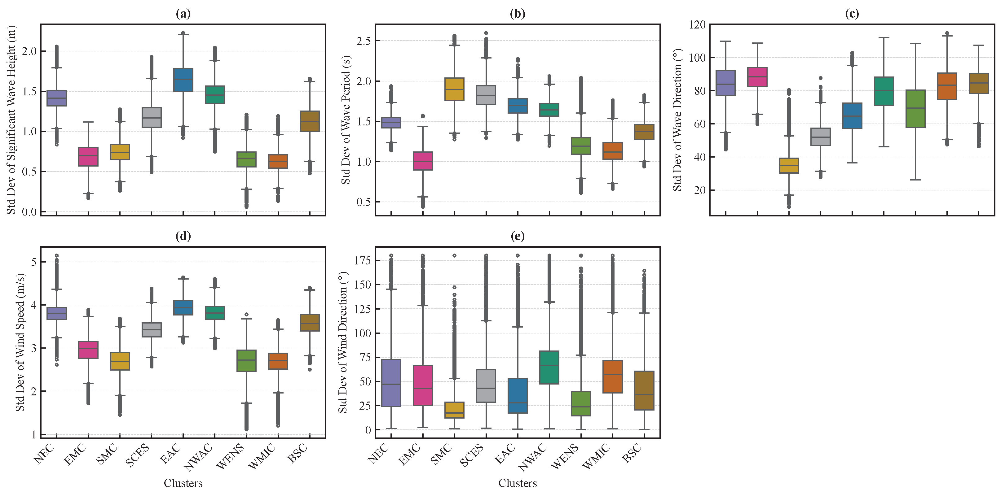
Transitional regimes (WMIC, WENS) and the southern Mediterranean (SMC) occupy an intermediate band. WMIC has the broadest spread among these, WENS is moderate, and SMC is comparatively tight. The annual standard deviation boxplots (Figure A3a) mirror this hierarchy: largest dispersion in NWAC/EAC, smallest in EMC/BSC (with SCES slightly higher), and intermediate over WMIC/WENS/SMC.
The open-ocean signal reflects persistent exposure to North Atlantic storm tracks and long-fetch swell, elevating both mean levels and variability in NWAC/EAC; NEC remains elevated but more tempered. In enclosed basins, limited fetch and predominantly local forcing suppress wave growth and compress the distributions. Transition regimes blend these influences: WMIC/WENS carry Atlantic energy but are modulated by shelf processes, while SMC shows relatively uniform regional forcing.
From a metocean standpoint, NWAC/EAC require wider design and operational ranges due to their larger intrinsic variance and heavier upper tails; EMC/BSC offer more stable sea states suitable for sheltered operations. Transition regimes warrant case-specific treatment: neither purely open-ocean nor enclosed, they combine basin-scale exposure with regional heterogeneity. Together, panels (a) in Figure A2 and Figure A3 define a clear, physically grounded hierarchy used throughout the analysis.
3.3.2. Multi-Year Annual Distributions: Mean Wave Period ()
The annual distribution of mean wave period () shows a consistent hierarchy across regimes (Figure A2b). Open-Atlantic clusters, NWAC and EAC, followed by NEC, exhibit the longest periods with broad interquartile ranges and frequent upper-tail values, consistent with persistent swell influence. Enclosed and semi-enclosed basins (EMC, BSC, SCES) display shorter periods with compact spreads, reflecting locally forced seas. Transitional shelves (WMIC, WENS) and the southern Mediterranean (SMC) occupy an intermediate position: medians lie between the open-ocean and enclosed groups, and spreads are moderate.
The corresponding annual standard deviation panel (Figure A3b) reinforces these contrasts. Variability in is largest in the open-Atlantic (NWAC, EAC), intermediate over the transitional shelves (WMIC, WENS) and SMC, and smallest within the enclosed basins (EMC, BSC, SCES). NEC typically falls between the open-Atlantic and transitional groups, reflecting partial continental influence along the Nordic–Barents margins.
Within the Atlantic, NWAC and EAC consistently lead in both median and spread, while NEC remains slightly shorter and less variable. Among transitional regimes, WMIC often shows a broader range than WENS, consistent with exposure to both Atlantic swell and Iberian/Mediterranean winds. SMC tends toward the tighter end of the transitional group, with medians closer to the enclosed basins than to the open-Atlantic.
The ordering of reflects fundamental fetch and forcing controls. Long periods and larger spreads in the open-Atlantic arise from recurrent, long-fetch storm systems and the prevalence of mature swell. Compact, shorter periods in enclosed basins follow from limited fetch and dominant local wind sea generation. Transitional shelves blend these behaviours: mixed sea–swell conditions produce intermediate medians and moderate variance.
Together, , , wave direction, and local wind statistics help distinguish regions where swell, wind sea, or a mixture of both is likely to dominate. Longer periods and differences between wind and wave directions generally indicate remotely generated swell, whereas shorter periods and closer wind–wave alignment are more typical of locally generated seas. The seasonal and annual means describe the typical conditions, while the standard deviations show their variability. However, because we use total-sea parameters, wind sea and swell cannot be quantified separately, and crossing wave systems cannot be resolved.
Because wave period modulates wave energy flux and near-bed orbital velocities, these contrasts have practical implications for design and operations. Longer, more variable periods in NWAC and EAC imply wider energy-bearing frequency bands and more stringent fatigue and response checks. By contrast, the shorter, more stable periods in EMC, BSC, and SCES support narrower design spectra and steadier operability envelopes. The transitional shelves require hybrid treatment, with allowance for episodic swell superimposed on locally forced seas.
3.3.3. Multi-Year Annual Distributions: Wind Speed ()
Annual 10 m wind speed () shows a clear spatial ordering across regimes (Figure A2d). Open-Atlantic clusters NWAC and EAC, with NEC trailing, exhibit the highest medians and broad interquartile ranges. Enclosed and semi-enclosed basins (EMC, BSC, SCES) present lower medians with compact spreads. Transitional shelves (WMIC, WENS) and the southern Mediterranean (SMC) occupy an intermediate band.
The annual standard deviation panel for (Figure A3d) mirrors the mean pattern: variability is largest over NWAC and EAC, intermediate over WMIC, WENS and SMC, and smallest within EMC, BSC and SCES. NEC typically sits between the Atlantic core (NWAC/EAC) and the transitional group.
Within the Atlantic, NWAC generally shows the widest spread, consistent with frequent cyclones and strong winter variability, while EAC maintains similarly high medians with slightly tighter dispersion. WENS tends to be windier than WMIC (North Sea exposure), and SMC sits at the lower end of the transitional cohort.
Spatial contrasts in shape wind sea growth, operability windows, and design envelopes. Higher and more variable winds in NWAC and EAC call for broader environmental design spectra and conservative weather-risk management; tighter, lower-wind climates in EMC, BSC, and SCES support narrower operability bands; transitional shelves require hybrid strategies that accommodate episodic Atlantic influence.
3.3.4. Multi-Year Annual Distributions: Wave Direction ()
Annual mean wave direction () shows coherent, regime-specific centres across all nine clusters (Figure A2c). The open-Atlantic domains NWAC and EAC exhibit tightly grouped medians within a consistent sector, reflecting persistent swell approach from the Atlantic storm track. NEC is similarly well organised but with a slight rotation relative to NWAC and EAC, consistent with Norwegian–Barents Sea exposure. Enclosed and semi-enclosed basins (EMC, BSC, SCES) display compact central angles, strongly constrained by basin geometry and limited fetch. Transitional shelves (WMIC, WENS) and the southern Mediterranean (SMC) occupy intermediate positions: their medians remain stable across years but spread more than the enclosed basins and less than the Atlantic core, evidencing the mixed influence of swell and locally forced seas.
The dispersion panel (Figure A3c) follows the same ordering. Directional variability is largest in the open ocean (NWAC, EAC), reflecting multiple storm approaches and occasional regime shifts, while NEC is moderate. Among the transitional shelves, WMIC typically shows the broadest spread (Atlantic–Mediterranean interface and coastal steering), with WENS somewhat tighter (North Sea shelf orientation). SMC sits in the intermediate-to-low range. The enclosed and semi-enclosed basins (EMC, BSC, SCES) exhibit the smallest dispersion, consistent with short fetch and boundary control.
All direction panels use circular statistics: circular means are reported after wrapping angles to , and variability is quantified with a circular spread measure, avoiding artificial widening near the seam. The persistent sectoral medians in NWAC, EAC, and NEC indicate stable swell approach at the annual scale, whereas the compact spreads in EMC, BSC, and SCES reflect fetch limitation and boundary effects. Transitional shelves (WMIC, WENS) show mixed signals that are physically credible given their dual exposure. Together, these patterns confirm that the directional climatology encoded by the clusters is geographically coherent and dynamically consistent with known forcing.
3.3.5. Multi-Year Annual Distributions: Wind Direction ()
Annual mean 10 m wind direction () exhibits coherent, regime-specific sectors across the nine clusters (Figure A2e). The open-Atlantic domains NWAC and EAC are westerly centred with broad spreads, consistent with frequent synoptic passages and long storm-track fetch; this variability underpins the elevated and longer observed in these regimes. NEC is similarly organised but rotated relative to NWAC and EAC, reflecting Norwegian–Barents exposure. Enclosed and semi-enclosed basins (EMC, BSC, SCES) show compact directional envelopes constrained by basin geometry and limited fetch. Transitional shelves (WMIC, WENS) and the southern Mediterranean (SMC) occupy intermediate positions: medians are stable but spreads exceed those of enclosed basins and are smaller than in the Atlantic core, consistent with mixed local and swell-related forcing.
The variability panel (Figure A3e) follows the same ordering. Directional variability is largest in NWAC and EAC, moderate in NEC, intermediate over WMIC and WENS (with WMIC typically broader given its Atlantic–Mediterranean interface), and smallest in EMC, BSC, and SCES; SMC sits in the intermediate-to-low range. All statistics are circular, with means wrapped to and spread measured using circular dispersion.
These contrasts are operationally relevant. Broader directional variability in NWAC, EAC, and parts of WMIC implies wider metocean load roses, larger yaw/heading excursions, and tighter fatigue allowances. Narrow spreads in EMC, BSC, and SCES support tighter design sectors and more stable operability windows. In transitional shelves such as WMIC and WENS, seasonal wind rotation increases the likelihood of reversals in wave approach and alongshore sediment transport, requiring case-specific coastal planning. SMC, though transitional, behaves closer to enclosed seas, supporting more persistent directional regimes. Because directional spread is greatest where synoptic variability dominates, anomalies linked to North Atlantic modes are most visible in NWAC and EAC and at the Atlantic–Mediterranean interface (WMIC), whereas enclosed basins exhibit higher year-to-year predictability of approach direction. Any long-term displacement of the storm track or westerly jet would be expected to manifest first as shifts in mean sector or dispersion in NWAC and EAC; the cluster climatology here provides a baseline for such monitoring.
3.3.6. Short-Term and Interannual Variability
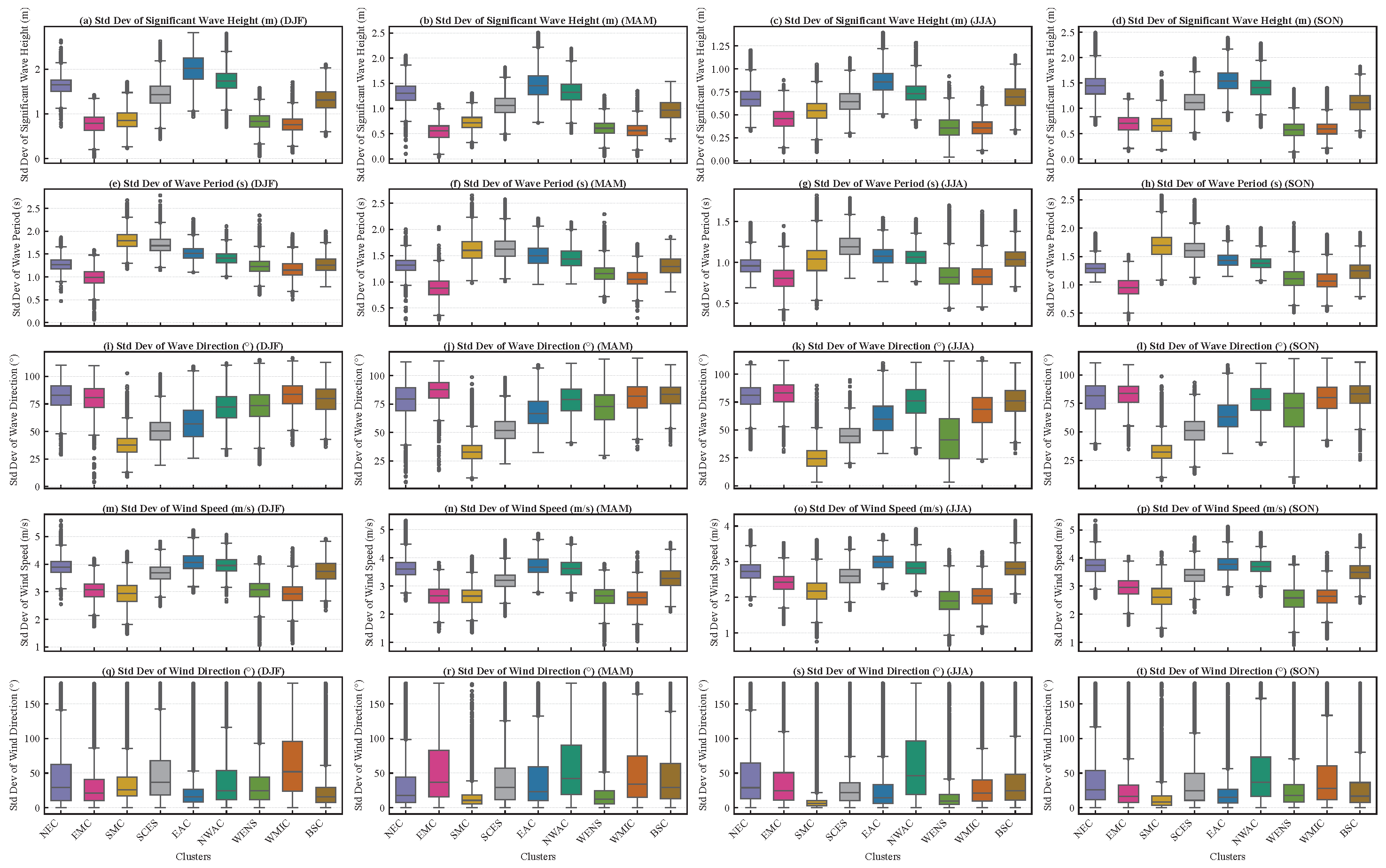
We quantify the seasonal cycle and year-to-year variability using seasonal means and seasonal standard deviations for all variables (Figure A4 and Figure A5). Seasonal means describe the intra-annual structure (DJF, MAM, JJA, SON); seasonal standard deviations summarise interannual spread within each season over 1979–2014.
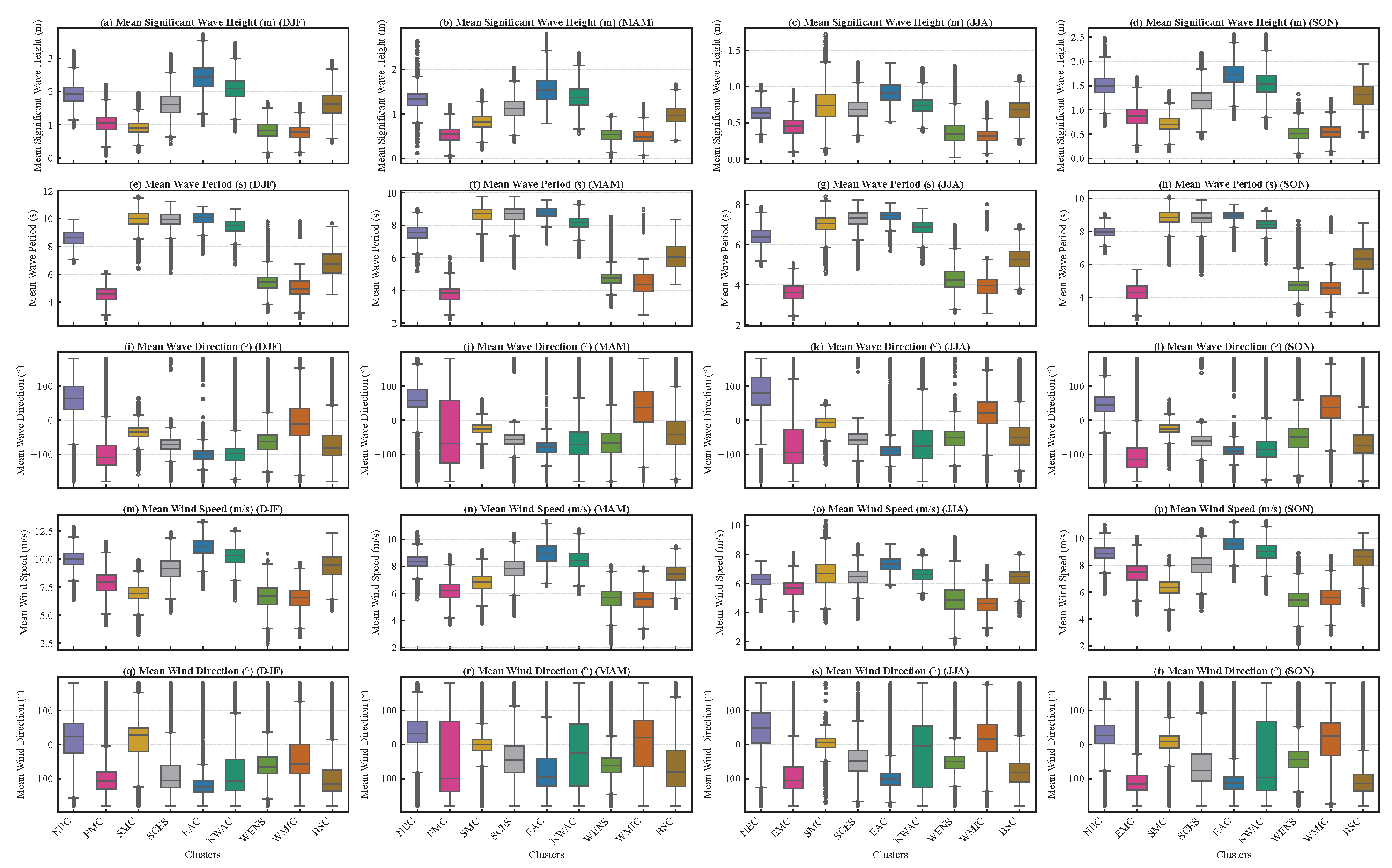
Significant wave height (): Open-Atlantic regimes (NWAC, EAC, NEC) peak in DJF and minimise in JJA, with broad winter distributions (Figure A4a). Enclosed basins (EMC, SCES, BSC) show lower amplitudes and tighter spreads across all seasons. Transitional shelves (WMIC, WENS) are intermediate; SMC is comparatively compact.
Wave period (): The seasonal ordering mirrors (Figure A4b): longer periods in DJF for NWAC and EAC (swell-rich conditions), shorter in JJA. Enclosed clusters retain shorter, less variable periods throughout the year.
Wind speed (): DJF maxima in open-ocean clusters with a marked summer minimum (Figure A4d). Enclosed clusters show muted seasonality; transitional shelves sit between.
Wave direction () and wind direction (): Open-ocean clusters retain westerly dominated sectors, most concentrated in DJF and broader in shoulder seasons (Figure A4c,e). Transitional shelves (WMIC, WENS) exhibit clear seasonal rotation (backing/veering) of prevailing sectors. Enclosed basins maintain narrower, more persistent approach and wind sectors across seasons.
and variability: Seasonal standard deviations are largest in DJF for NWAC, EAC, and NEC and smallest in JJA, with enclosed basins lowest in all seasons (Figure A5a,b). Transitional shelves are mid-range; SMC remains relatively low.
variability: The same winter-high/summer-low ordering holds (Figure A5d), strongest over the open-Atlantic and weakest in enclosed basins.
Directional variability (circular spread): Directional standard deviations are generally larger outside winter (often MAM/SON) in open-ocean and transitional regimes, and smallest year-round in enclosed basins (Figure A5c,e). Winter sectors are typically tighter over NWAC and EAC, with cluster-specific exceptions (e.g., episodic winter broadening in transitional shelves).
The winter maxima and broad spreads in , , and over NWAC, EAC, and NEC reflect the seasonal strengthening and meridional excursions of the North Atlantic storm track, longer effective fetch, and frequent swell incidence. Conversely, the compact seasonal envelopes in EMC, SCES, and BSC arise from geometric confinement and locally forced, short-sea conditions. Transitional shelves (WMIC, WENS) express both behaviours: winter exposure to Atlantic systems and seasonal rotation of prevailing sectors, which broadens directional spread in the shoulder seasons and moderates it in DJF/JJA. The persistently low spread in SMC is consistent with more coherent regional forcing relative to the western/central Mediterranean interface.
Taken together, the seasonal means set the expected cycle (energetic in winter, quiescent in summer) and the seasonal standard deviations indicate where that cycle is most variable from year to year: high over the open-Atlantic in DJF, moderate over transitional shelves, and low in enclosed basins. The directional panels confirm that clusters differ not only in energy level but also in directional persistence versus sectoral rotation, which is central for wave growth, coastal transport, and design load envelopes.
3.4. Teleconnection Imprints on Regional Wind–Wave Clusters
We examine associations between seasonal and annual wind–wave metrics and two groups of teleconnection indices: Group 1 (NAO, SCAND, EA, EAWR) and Group 2 (AO, PNA, POLEUR, WP). Spearman rank correlations were first calculated at each grid cell for every climate index–variable–period combination. Grid cell correlations with two-tailed were retained and subsequently averaged within each cluster for every climate index. Figure 5 and Figure 6 display all indices for which the mean of the retained grid cell correlations satisfies . When multiple indices meet this threshold within the same cluster–variable cell, all are reported, while the background colour represents the coefficient with the largest absolute magnitude. Empty cells indicate that no index met the display threshold.
Figure 5.
Group 1 teleconnections (NAO = N, SCAND = S, EA = E, EAWR = W): dominant correlations summarised by wind–wave regime. Spearman rank correlations were calculated at each grid cell for every climate index–variable–period combination, and coefficients with two-tailed were retained. For each cluster, variable–period combination, and climate index, the retained grid cell coefficients were averaged to obtain . Each cell lists all indices for which , while the background colour represents the coefficient with the largest absolute magnitude among those displayed (red = positive; blue = negative). Empty cells indicate that no index met the display threshold. Directional variables ( and ) were treated using sine and cosine projections before calculating the Spearman associations. The results are based on ERA5 for 1979–2014 and clusters.
Figure 6.
Group 2 teleconnections (PNA = P, WP = WP, POLEUR = R, AO = A): dominant correlations summarised by wind–wave regime. Spearman rank correlations were calculated at each grid cell for every climate index–variable–period combination, and coefficients with two-tailed were retained. For each cluster, variable–period combination, and climate index, the retained grid cell coefficients were averaged to obtain . Each cell lists all indices for which , while the background colour represents the coefficient with the largest absolute magnitude among those displayed (red = positive; blue = negative). Empty cells indicate that no index met the display threshold. Directional variables ( and ) were treated using sine and cosine projections before calculating the Spearman associations. The results are based on ERA5 for 1979–2014 and clusters.
Climate indices represent large-scale modes of atmospheric circulation and do not themselves directly force the wave field. Instead, their associated pressure anomalies modify regional pressure gradients, jet-stream position, cyclone trajectories, and storm persistence. The resulting changes in surface wind speed, direction, duration, and effective fetch influence local wave generation and growth. Changes in storm location and sequencing can also affect remotely generated swell, including its period and approach direction [18,31,32]. Accordingly, coherent associations in and are interpreted primarily as changes in local or regional wind forcing, whereas changes in without a comparable response in may reflect changes in storm duration, source region, or swell propagation. Associations with directional variables provide information about phase-dependent changes in prevailing wind and wave sectors. Even though the directional analysis is based on sine and cosine projections, the sign of the retained coefficient should not by itself be interpreted as a clockwise or anticlockwise rotation. These physical pathways provide the basis for interpreting the statistical relationships discussed below.
3.4.1. Group 1: NAO, SCAND, EA, and EAWR
Figure 5 reveals spatially and seasonally heterogeneous associations across the nine wind–wave regimes. Among the Group 1 indices, the NAO produces the most prominent associations in the open-Atlantic clusters. In EAC, the NAO is positively associated with annual and winter ( and , respectively), spring (), and spring (). In NEC, positive NAO associations occur for spring , , and (, , and , respectively). Strong NAO associations are also found for wave direction in NEC during MAM, JJA, and SON (, , and ) and for wind direction during MAM, JJA, and SON (, , and ). The NAO is negatively associated with in NEC during SON () and in WENS during JJA (), indicating that its relationship with wave period varies by region and season. In NWAC, the strongest NAO relationships are directional, particularly for summer wave direction () and spring–summer wind direction ( and ). Because the directional analysis uses sine and cosine projections, these coefficient signs indicate statistical associations with the directional components and should not be interpreted directly as clockwise or anticlockwise rotations.
The strongest opposing response occurs in WENS during DJF. Here, the NAO is positively associated with both and ( and ), whereas EAWR is negatively associated with the same variables ( and ). Winter in WENS is also positively associated with the NAO and EA ( and ). This result identifies WENS as a region where different circulation modes are associated with contrasting winter wind and wave conditions.
SCAND has its clearest imprint in the Baltic cluster (BSC). Higher SCAND values are associated with lower autumn , , and (, , and , respectively). SCAND also exhibits strong associations with wave direction in MAM and SON ( and ) and wind direction in the same seasons ( and ). EA produces an opposing autumn directional association in BSC, with coefficients of for wave direction and for wind direction. Outside the Baltic, SCAND is negatively associated with autumn and in NEC (both approximately ).
EA and EAWR generally produce more localised associations. EA is positively associated with winter in WENS () and summer in SMC (). In WMIC, EA is associated with spring wave direction (), winter (), and wind direction during DJF, MAM, and SON (, , and ). EAWR is positively associated with winter and in NEC ( and ), but negatively associated with these variables in WENS, as noted above. Additional EAWR associations include winter in EMC (), autumn wave direction in SMC (), and summer in BSC (). No cluster-mean coefficient in SCES exceeds the display threshold. This does not demonstrate an absence of teleconnection influence, but indicates that no association satisfied the selected criterion after the cluster-level averaging procedure.
The observed associations can be interpreted through the atmospheric circulation patterns represented by these indices. During a positive NAO phase, the intensified pressure difference between the Icelandic Low and the Azores High modifies the strength and position of the North Atlantic westerlies and storm track [6]. The resulting changes in surface wind speed, storm persistence, and effective fetch provide a physical explanation for the coherent and associations in EAC, NEC, and WENS. Changes in storm trajectory and duration can additionally modify the source and propagation of swell, helping to explain why the sign of the association varies among seasons and regions [18,31,32]. The opposing NAO and EAWR relationships in WENS are consistent with the different ways in which these circulation modes modify the atmospheric pressure gradient and storm activity over the European shelf.
The SCAND pattern is associated with atmospheric blocking over northern Europe, which can redirect cyclone trajectories and alter the regional wind field. In the fetch-limited Baltic Sea, even modest changes in wind direction can substantially change the distance over which waves develop. This provides a plausible mechanism for the simultaneous SCAND associations with autumn wind speed, wave height, wave period, and directional variables. In the Mediterranean clusters, the more localised EA and EAWR relationships are consistent with the influence of basin geometry, surrounding topography, and regional winds, which can limit the extent to which large-scale circulation anomalies produce spatially coherent wave responses. These mechanisms are physically consistent with the observed correlations, although the correlation analysis alone does not establish causality.
From an applied perspective, the relationships suggest that teleconnection phase could be used as a covariate when stratifying seasonal metocean conditions. The particularly clear winter response in WENS and the annual and winter associations in EAC may be relevant to assessments of offshore accessibility and operating conditions. In BSC, the strong SCAND relationships with directional variables suggest that phase-conditioned wave and wind sectors may be relevant to layout, mooring, and navigation assessments. However, the present analysis evaluates associations in mean wind–wave conditions and does not directly quantify extreme waves, structural loads, or operational downtime. Applying these results to design limits would therefore require a separate phase-conditioned analysis of extremes and engineering response.
3.4.2. Group 2: PNA, WP, POLEUR, and AO
Figure 6 shows the Group 2 associations retained after filtering the grid cell correlations at two-tailed . The displayed values are cluster means of the retained coefficients that satisfy . Among these indices, the AO has the broadest spatial and multivariate footprint, particularly in NEC and EAC.
In NEC, the AO is positively associated with on annual, DJF, MAM, and SON timescales (, , , and , respectively). Positive associations are also found for annually and during DJF and MAM (, , and ) and for annually and during DJF, MAM, and SON (, , , and ). Directional associations occur for wave direction during MAM, JJA, and SON (, , and ) and for wind direction during JJA and SON (both ).
A similarly coherent, although less extensive, AO response is found in EAC. Here, the AO is positively associated with annual and winter ( and ), annual, winter, and spring (, , and ), and annual (). The spring wave direction coefficient is negative (). As in the Group 1 analysis, the signs of the directional coefficients describe associations with the selected sine or cosine component and should not be interpreted directly as clockwise or anticlockwise rotations.
The AO associations in the remaining clusters are more selective. In NWAC, the AO is positively associated with winter () and negatively associated with summer wave direction () and wind direction during JJA and SON ( and ). In WMIC, positive AO associations occur for autumn and ( and ), together with annually, in DJF, and in MAM (, , and ). In BSC, the displayed AO response is confined to on annual and DJF timescales ( and ). SMC exhibits positive AO associations with spring (), autumn (), and spring wind direction ().
PNA, POLEUR, and WP produce fewer associations and are confined to WENS at the selected threshold. During DJF, is negatively associated with PNA () and positively associated with POLEUR (). WP is negatively associated with spring (), while POLEUR is positively associated with autumn (). The only displayed AO association in WENS is for winter wave direction (). No Group 2 cluster-mean coefficient in EMC or SCES exceeds the display threshold.
The broad AO imprint in NEC and EAC is physically consistent with its influence on the large-scale pressure gradient, circumpolar circulation, and North Atlantic storm track. During positive AO conditions, changes in the strength and position of the westerly circulation can modify regional surface winds, cyclone trajectories, storm persistence, and effective fetch [6]. The coherent positive associations among , , and in NEC and EAC are therefore consistent with enhanced or more persistent wind forcing and wave development. The AO associations with may additionally reflect changes in storm duration and swell-source location, while the directional associations indicate that the prevailing wind and wave sectors vary with the large-scale circulation state [18,31,32].
The period-centred PNA, POLEUR, and WP associations in WENS suggest a different pathway. These indices cannot directly generate ocean swell over the European shelf. Instead, their atmospheric circulation patterns can affect Rossby-wave propagation, jet-stream configuration, and subsequent cyclone activity over the North Atlantic–European sector. Changes in storm trajectory, persistence, and sequencing can alter the location and duration of wave generation and therefore affect without producing an equally strong response in . The opposing winter associations with PNA and POLEUR suggest that the two circulation patterns project differently onto the atmospheric pathways controlling swell generation and propagation toward WENS. These mechanisms provide a physically plausible interpretation of the correlations but do not establish direct causality.
The absence of displayed Group 2 associations in EMC and SCES should not be interpreted as evidence that these indices have no influence. Rather, the relationships may be weaker than the selected threshold, spatially heterogeneous within the clusters, or masked by local and regional forcing. This interpretation is particularly relevant to enclosed and semi-enclosed seas, where basin geometry, restricted fetch, topography, and regional wind systems can modify the response to large-scale atmospheric circulation.
From an applied perspective, the AO associations in NEC and EAC suggest that AO phase may be a useful covariate when stratifying seasonal metocean conditions for offshore planning and accessibility assessments. The more selective AO responses in NWAC, WMIC, BSC, and SMC indicate that the relevant variables and seasons differ among regimes. In WENS, phase-conditioned analyses of wave period distributions may help determine whether the PNA, POLEUR, and WP relationships affect operational or structural response. However, the present results describe associations in mean conditions and do not directly quantify extreme waves, fatigue damage, mooring loads, or downtime. Such engineering applications would require separate analyses of conditional extremes, wave spectra, and structural response.
3.5. Comparison with Previous Wave Climate Classifications
The broad organisation of the regimes identified here is consistent with previous wave climate studies, although a direct correspondence is not expected because earlier classifications used different variables, domains, and objectives (Table A1). The separation of NWAC, EAC, and NEC as energetic, swell-exposed Atlantic regimes agrees with the open-ocean conditions described by Semedo et al. [31] and the high-energy classes identified by Fairley et al. [25]. Similarly, the distinction between WENS and BSC is consistent with the contrasting North Sea and Baltic wave climates reported by Bonaduce et al. [15]. The separation of WMIC, SMC, EMC, and SCES supports previous evidence that the Mediterranean contains marked sub-basin differences associated with regional winds, basin geometry, and wind sea–swell interactions [7,12]. For teleconnections, the broad NAO response and more regional SCAND and EAWR associations agree with Martínez-Asensio et al. [18], although the present analysis additionally identifies a broad AO imprint and period-centred PNA, POLEUR, and WP associations in WENS. Unlike earlier wave-only or region-specific classifications, the present regimes integrate multiple wind and wave parameters and their complete seasonal and interannual behaviour. A detailed comparison is provided in Appendix A.3, Table A1.
4. Summary and Conclusions
We classified multivariate wind–wave regimes across European seas using ERA5 data for 1979–2014 at resolution. Seasonal and annual means and standard deviations were calculated for significant wave height (), mean wave period (), 10 m wind speed (), and wave and wind directions, with circular statistics used for the directional variables. PCA retained 30 components explaining approximately 99% of the variance, and k-means clustering identified nine regional regimes. For each grid cell, the yearly principal component scores were concatenated over the complete 36-year period before clustering. The resulting clusters therefore represent persistent multi-decadal wind–wave behaviour rather than conditions in individual years.
The nine regimes show a clear separation between the open-Atlantic, transitional shelves, and enclosed or semi-enclosed seas. Open-Atlantic regimes have higher and more variable , , and , with pronounced winter maxima and broader directional variability. Enclosed basins have lower variability, shorter wave periods, and wind and wave directions that are more strongly constrained by basin geometry. Transitional regions combine Atlantic exposure with locally generated wind seas and show intermediate conditions and seasonal directional changes. The cluster-distance analysis supports this organisation: EAC and SMC are the most internally compact regimes, while EMC, SCES, and BSC are more heterogeneous. The largest differences occur between EAC and the transitional or Mediterranean regimes, whereas WMIC and WENS form the most similar pair.
The relationships with large-scale atmospheric circulation vary by region, variable, and season. NAO shows the broadest Group 1 associations in the Atlantic and European shelf regions, while SCAND has its clearest associations in the Baltic and EA and EAWR act more locally. AO has the broadest Group 2 associations, particularly in NEC and EAC, with more selective associations in the other regimes. At the selected threshold, the PNA, POLEUR, and WP relationships are confined to wave period variability in WENS. Changes in pressure gradients, jet-stream position, cyclone tracks, surface winds, and effective fetch provide a physically plausible explanation for these patterns. However, the results show statistical associations and do not establish direct causal relationships.
- Practical Implications
(1) Zoning and siting. The regimes provide regional units for preliminary resource comparison and planning. They distinguish the energetic and highly variable open-Atlantic regimes (NWAC/EAC), the intermediate conditions of the transitional shelves (WENS/WMIC), and the lower-energy, less variable conditions of the enclosed basins (EMC/SCES/BSC). (2) Design and operations. The associations between NAO/AO and , , and suggest that circulation phase may be a useful covariate in seasonal metocean assessment and maintenance planning, particularly in NEC and EAC. In WENS, the relationships of PNA, POLEUR, and WP with indicate that phase-conditioned wave period and spectral analyses may be relevant to fatigue and accessibility assessments. The SCAND associations with directional conditions in BSC may also be relevant to layout, alignment, and navigation planning. These possible applications require separate analyses of extremes, wave spectra, and engineering response. (3) Monitoring. Climate indices may provide additional context for interpreting seasonal and interannual changes in regional wind–wave conditions. In particular, NAO and AO are relevant to NEC and EAC, while PNA, POLEUR, and WP may help interpret wave period variability in WENS.
Beyond annual means, seasonality provides additional structure to observed variability. Open-Atlantic regimes peak in winter and relax in summer, with broader year-to-year variability than in enclosed basins, which remain compact and predictable across seasons. Transitional shelves combine both influences: winter exposure to Atlantic storms and seasonal rotation of prevailing sectors. Directional contrasts are equally important: broad, variable sectors in NWAC/EAC pose design challenges, narrow envelopes in EMC/BSC/SCES support stable directional assumptions, and WMIC/WENS highlight the role of seasonal reversals. Together, these results extend the classification from annual averages to dynamic seasonal regimes, directly relevant for design spectra, coastal planning, and long-term monitoring.
- Scope and Next Steps
The reported correlations are statistical and based on cluster means with strict thresholds, which may smooth smaller-scale signals. In addition, k-means assumes approximately spherical cluster geometry, although the PCA representation and validation metrics support an interpretable solution within the present dataset. An important limitation is that the complete analysis is based on ERA5. The feature set sensitivity analysis does not quantify between-product uncertainty, and the identified regimes should therefore be regarded as an ERA5-based classification rather than fixed, dataset-independent geographical divisions.
Future work should (i) extend the analysis to sub-cluster scales, (ii) incorporate hindcast, altimetry and spectral information, (iii) test nonlinear embeddings and alternative clustering methods, (iv) propagate the regime framework into climate projections, and (v) repeat the complete workflow using independent wind and wave reanalysis or hindcast products. Cross-dataset robustness could then be quantified by comparing cluster membership, regime boundaries, centroid characteristics, and spatial agreement across products.
Author Contributions
P.M.: Conceptualisation, Data curation, Formal analysis, Investigation, Methodology, Software, Validation, Visualisation, Writing—original draft. J.A.A.A.: Conceptualisation, Methodology, Resources, Supervision, Validation, Writing—review and editing. K.P.: Validation, Writing—review and editing. L.C.: Writing—review and editing. A.V.M.: Funding acquisition, Project administration, Supervision, Writing—review and editing. All authors have read and agreed to the published version of the manuscript.
Funding
This research received no external funding.
Data Availability Statement
Publicly available datasets were analysed in this study. ERA5 hourly single-level data are available from the Copernicus Climate Data Store at https://cds.climate.copernicus.eu/datasets/reanalysis-era5-single-levels (accessed on 1 August 2026). Monthly teleconnection indices are available from the Climate Prediction Center of the National Oceanic and Atmospheric Administration (NOAA) at https://www.cpc.ncep.noaa.gov/data/teledoc/telecontents.shtml (accessed on 1 August 2026). The processed data and analysis code are available from the corresponding author upon reasonable request.
Acknowledgments
Special thanks are extended to the European Centre for Medium-Range Weather Forecasts (ECMWF) for making the ERA5 reanalysis dataset available, which was instrumental in our analysis. The indices were sourced from the National Centers for Environmental Prediction (NCEP), and their integration significantly enhanced the analysis of climate oscillations. We also appreciate the constructive feedback from our colleagues in the Offshore Engineering and Coastal Engineering groups, whose insights have significantly enhanced the quality of this work. Any use of trade, firm, or product names is for descriptive purposes only and does not imply endorsement by the U.S. Government.
Conflicts of Interest
The authors declare no conflicts of interest.
Correction Statement
This article has been republished with a minor correction to the existing affiliation information and acknowledgments. This change does not affect the scientific content of the article.
Appendix A. Supporting Distributions and Diagnostics
This appendix provides diagnostics and full distributions that support the summary figures discussed in the main text. Appendix figures are labelled as Figure A1 and Figure A2, etc.
Appendix A.1. Cluster Variability Diagnostics
Figure A1 shows the full distributions of Euclidean distances from grid cells to their assigned cluster centroids in the 1080-dimensional concatenated PC-score space. This complements the boxplot summary in the main text (Figure 3) by illustrating distribution shape and tail behaviour within each regime.
Figure A1.
Intra-cluster distance distributions (ERA5, ). Histograms of Euclidean distances from each grid cell to its cluster centroid in the 1080-dimensional concatenated PC-score space (dimensionless). Dashed lines indicate cluster means; panel titles list regime and sample size n.
Appendix A.2. Annual Distributions
Figure A2 and Figure A3 provide the full annual distributions by cluster that underpin the regime-level comparisons in Section 3.3.
Figure A2.
Annual mean distributions by cluster (ERA5, 1979–2014; ). Boxplots of annual mean values of (a) , (b) , (c) , (d) , and (e) . Boxes show medians and interquartile ranges; whiskers denote ; points indicate outliers. Directional means use circular statistics with angles wrapped to .
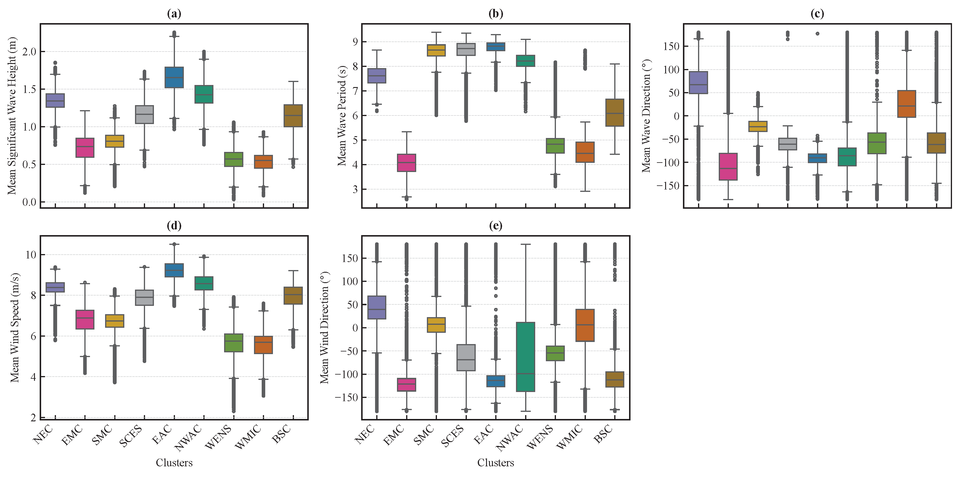
Figure A3.
Annual variability (standard deviation) by cluster (ERA5, 1979–2014; ). Boxplots of annual standard deviations for (a) , (b) , (c) (circular s.d.), (d) , and (e) (circular s.d.). Boxes show medians and interquartile ranges; whiskers denote ; points indicate outliers.
Appendix A.3. Comparison with Previous Wave Climate Classifications
Table A1.
Qualitative comparison between the wind–wave regimes identified in this study and regional structures reported in previous wave climate studies. The correspondence is conceptual rather than a direct reproduction of earlier boundaries because the studies use different variables, spatial scales, and classification objectives.
Appendix A.4. Seasonal Mean Distributions
Figure A4 provides the full seasonal mean distributions (DJF, MAM, JJA, SON) for all variables and clusters. This supports the seasonal discussion in Section 3.3.
Figure A4.
Seasonal means by cluster (ERA5, 1979–2014; ). Boxplots of seasonal mean values for five variables across the nine clusters. Columns correspond to seasons (DJF, MAM, JJA, SON); rows correspond to , , , , and . Directional means use circular statistics. Boxes show medians and interquartile ranges; whiskers denote ; points indicate outliers.
Appendix A.5. Seasonal Variability Distributions
Figure A5 presents the full seasonal standard deviation distributions (DJF, MAM, JJA, SON) for all variables and clusters. This supports the seasonal variability discussion in Section 3.3.
Figure A5.
Seasonal variability by cluster (standard deviations; ERA5, 1979–2014; ). Boxplots of seasonal standard deviations for five variables across the nine clusters. Columns correspond to seasons (DJF, MAM, JJA, SON); rows correspond to , , (circular s.d.), , and (circular s.d.). Directional spreads use circular statistics. Boxes show medians and interquartile ranges; whiskers denote ; points indicate outliers.
References
- Reguero, B.G.; Losada, I.J.; Díaz-Simal, P.; Méndez, F.J.; Beck, M.W. Effects of Climate Change on Exposure to Coastal Flooding in Latin America and the Caribbean. PLoS ONE 2015, 10, e0133409. [Google Scholar] [CrossRef] [Scilit] [PubMed]
- Waterhouse, A.F.; MacKinnon, J.A.; Nash, J.D.; Alford, M.H.; Kunze, E.; Simmons, H.L.; Polzin, K.L.; Laurent, L.C.S.; Sun, O.M.; Pinkel, R.; et al. Global patterns of diapycnal mixing from measurements of the turbulent dissipation rate. J. Phys. Oceanogr. 2014, 44, 1854–1872. [Google Scholar] [CrossRef] [Scilit]
- Dodet, G.; Melet, A.; Ardhuin, F.; Bertin, X.; Idier, D.; Almar, R. The contribution of wind-generated waves to coastal sea-level changes. Surv. Geophys. 2019, 40, 1563–1601. [Google Scholar] [CrossRef] [Scilit]
- Hemer, M.A.; Church, J.A.; Hunter, J.R. Variability and trends in the directional wave climate of the Southern Hemisphere. Int. J. Climatol. A J. R. Meteorol. Soc. 2010, 30, 475–491. [Google Scholar] [CrossRef] [Scilit]
- Liang, J.H.; Wan, X.; Rose, K.A.; Sullivan, P.P.; McWilliams, J.C. Horizontal dispersion of buoyant materials in the ocean surface boundary layer. J. Phys. Oceanogr. 2018, 48, 2103–2125. [Google Scholar] [CrossRef] [Scilit]
- Hurrell, J.W.; Deser, C. North Atlantic climate variability: The role of the North Atlantic Oscillation. J. Mar. Syst. 2010, 79, 231–244. [Google Scholar] [CrossRef] [Scilit]
- Casas-Prat, M.; Sierra, J.P. Projected future wave climate in the NW Mediterranean Sea. J. Geophys. Res. Ocean. 2013, 118, 3548–3568. [Google Scholar] [CrossRef] [Scilit]
- Morim, J.; Hemer, M.; Wang, X.L.; Cartwright, N.; Trenham, C.; Semedo, A.; Young, I.; Bricheno, L.; Camus, P.; Casas-Prat, M.; et al. Robustness and uncertainties in global multivariate wind-wave climate projections. Nat. Clim. Change 2019, 9, 711–718. [Google Scholar] [CrossRef] [Scilit]
- Young, I.R.; Ribal, A. Multiplatform evaluation of global trends in wind speed and wave height. Science 2019, 364, 548–552. [Google Scholar] [CrossRef] [Scilit] [PubMed]
- Young, I.R.; Zieger, S.; Babanin, A.V. Global trends in wind speed and wave height. Science 2011, 332, 451–455. [Google Scholar] [CrossRef] [Scilit] [PubMed]
- Benetazzo, A.; Bergamasco, A.; Bonaldo, D.; Falcieri, F.M.; Sclavo, M.; Langone, L.; Carniel, S. Response of the Adriatic Sea to an intense cold air outbreak: Dense water dynamics and wave-induced transport. Prog. Oceanogr. 2014, 128, 115–138. [Google Scholar] [CrossRef] [Scilit]
- Elshinnawy, A.I.; Antolínez, J.A. A changing wave climate in the Mediterranean Sea during 58-years using UERRA-MESCAN-SURFEX high-resolution wind fields. Ocean Eng. 2023, 271, 113689. [Google Scholar] [CrossRef] [Scilit]
- Rodriguez-Delgado, C.; Bergillos, R.J.; Iglesias, G. Dual wave farms for energy production and coastal protection under sea level rise. J. Clean. Prod. 2019, 222, 364–372. [Google Scholar] [CrossRef] [Scilit]
- Bergillos, R.J.; Rodriguez-Delgado, C.; Iglesias, G. Ocean Energy and Coastal Protection: A Novel Strategy for Coastal Management Under Climate Change; Springer Nature: Cham, Switzerland, 2019. [Google Scholar] [CrossRef] [Scilit]
- Bonaduce, A.; Staneva, J.; Behrens, A.; Bidlot, J.R.; Wilcke, R.A.I. Wave climate change in the North Sea and Baltic Sea. J. Mar. Sci. Eng. 2019, 7, 166. [Google Scholar] [CrossRef] [Scilit]
- Lobeto, H.; Menendez, M.; Losada, I.J. Future behavior of wind wave extremes due to climate change. Sci. Rep. 2021, 11, 7869. [Google Scholar] [CrossRef] [Scilit] [PubMed]
- Varlas, G.; Vervatis, V.; Spyrou, C.; Papadopoulou, E.; Papadopoulos, A.; Katsafados, P. Investigating the impact of atmosphere–wave–ocean interactions on a Mediterranean tropical-like cyclone. Ocean Model. 2020, 153, 101675. [Google Scholar] [CrossRef] [Scilit]
- Martínez-Asensio, A.; Tsimplis, M.N.; Marcos, M.; Feng, X.; Gomis, D.; Jordà, G.; Josey, S.A. Response of the North Atlantic wave climate to atmospheric modes of variability. Int. J. Climatol. 2016, 36, 1210–1225. [Google Scholar] [CrossRef] [Scilit]
- Benetazzo, A.; Davison, S.; Barbariol, F.; Mercogliano, P.; Favaretto, C.; Sclavo, M. Correction of ERA5 Wind for Regional Climate Projections of Sea Waves. Water 2022, 14, 1590. [Google Scholar] [CrossRef] [Scilit]
- Acar, E.; Akpınar, A.; Kankal, M.; Amarouche, K. Wave Power Trends over the Mediterranean Sea Based on Innovative Methods and 60-Year ERA5 Reanalysis. Sustainability 2023, 15, 8590. [Google Scholar] [CrossRef] [Scilit]
- Neill, S.P. Wave Resource Characterization and Co-location with Offshore Wind in the Irish Sea. Renew. Energy 2024, 222, 119902. [Google Scholar] [CrossRef] [Scilit]
- Barkanov, E.; Penalba, M.; Martinez, A.; Martinez-Perurena, A.; Zarketa-Astigarraga, A.; Iglesias, G. Evolution of the European Offshore Renewable Energy Resource under Multiple Climate Change Scenarios and Forecasting Horizons via CMIP6. Energy Convers. Manag. 2024, 301, 118058. [Google Scholar] [CrossRef] [Scilit]
- Majidi, A.G.; Ramos, V.; Calheiros-Cabral, T.; Santos, P.R.; Das Neves, L.; Taveira-Pinto, F. Integrated Assessment of Offshore Wind and Wave Power Resources in Mainland Portugal. Energy 2024, 308, 132944. [Google Scholar] [CrossRef] [Scilit]
- Çalışır, E.; Amarouche, K.; Çakmak, R.E.; Akpınar, A. Performance assessment of 22 CMIP6 climate models for projecting wind climate and wind power over the Mediterranean Sea. Environ. Earth Sci. 2026, 85, 170. [Google Scholar] [CrossRef] [Scilit]
- Fairley, I.; Lewis, M.; Robertson, B.; Hemer, M.; Masters, I.; Horrillo-Caraballo, J.; Reeve, D.E. A classification system for global wave energy resources based on multivariate clustering. Appl. Energy 2020, 262, 114515. [Google Scholar] [CrossRef] [Scilit]
- Pérez, J.; Menéndez, M.; Méndez, F.J.; Losada, I.J. Evaluating the performance of CMIP3 and CMIP5 global climate models over the north-east Atlantic region. Clim. Dyn. 2014, 43, 2663–2680. [Google Scholar] [CrossRef] [Scilit]
- Odériz, I.; Silva, R.; Mortlock, T.R.; Mori, N.; Shimura, T.; Webb, A.; Padilla-Hernández, R.; Villers, S. Natural Variability and Warming Signals in Global Ocean Wave Climates. Geophys. Res. Lett. 2021, 48, e2021GL093622. [Google Scholar] [CrossRef] [Scilit]
- Lobeto, H.; Menendez, M.; Losada, I.J.; Hemer, M. The Effect of Climate Change on Wind-Wave Directional Spectra. Glob. Planet. Change 2022, 213, 103820. [Google Scholar] [CrossRef] [Scilit]
- Goharnejad, H.; Perrie, W.; Toulany, B.; Casey, M.; Zhang, M. Impacts of Climate Change on Seasonal Extreme Waves in the Northwest Atlantic Using a Spatial Neural Gas Clustering Method. J. Ocean Eng. Sci. 2023, 8, 367–385. [Google Scholar] [CrossRef] [Scilit]
- Zhao, G.; Li, D.; Yang, S.; Qi, J.; Yin, B. The Development of a Weather-Type Statistical Downscaling Model for Wave Climate Based on Wave Clustering. Ocean Eng. 2024, 304, 117863. [Google Scholar] [CrossRef] [Scilit]
- Semedo, A.; Sušelj, K.; Rutgersson, A.; Sterl, A. A global view on the wind sea and swell climate and variability from ERA-40. J. Clim. 2011, 24, 1461–1479. [Google Scholar] [CrossRef] [Scilit]
- Janssen, P.A.E.M. The Interaction of Ocean Waves and Wind; Cambridge University Press: Cambridge, UK, 2004. [Google Scholar]
- Guanche, Y.; Guanche, R.; Camus, P.; Mendez, F.J.; Medina, R. A multivariate approach to estimate design loads for offshore wind turbines. Wind Energy 2013, 16, 1091–1106. [Google Scholar] [CrossRef] [Scilit]
- Sarmiento, J.; Iturrioz, A.; Ayllón, V.; Guanche, R.; Losada, I.J. Experimental modelling of a multi-use floating platform for wave and wind energy harvesting. Ocean Eng. 2019, 173, 761–773. [Google Scholar] [CrossRef] [Scilit]
- Hersbach, H.; Bell, B.; Berrisford, P.; Hirahara, S.; Horányi, A.; Muñoz-Sabater, J.; Nicolas, J.; Peubey, C.; Radu, R.; Schepers, D.; et al. The ERA5 global reanalysis. Q. J. R. Meteorol. Soc. 2020, 146, 1999–2049. [Google Scholar] [CrossRef] [Scilit]
- Reguero, B.G.; Losada, I.J.; Méndez, F.J. A global wave power resource and its seasonal, interannual and long-term variability. Appl. Energy 2015, 148, 366–380. [Google Scholar] [CrossRef] [Scilit]
- Eyring, V.; Bony, S.; Meehl, G.A.; Senior, C.A.; Stevens, B.; Stouffer, R.J.; Taylor, K.E. Overview of the Coupled Model Intercomparison Project Phase 6 (CMIP6) Experimental Design and Organization. Geosci. Model Dev. 2016, 9, 1937–1958. [Google Scholar] [CrossRef] [Scilit]
- Fanti, V.; Ferreira, Ó.; Kümmerer, V.; Loureiro, C. Improved Estimates of Extreme Wave Conditions in Coastal Areas from Calibrated Global Reanalyses. Commun. Earth Environ. 2023, 4, 151. [Google Scholar] [CrossRef] [Scilit]
- Patra, A.; Oueslati, B.; Chevallier, T.; Renaud, P.; Kervella, Y.; Dubus, L. Evaluation of ERA5, COSMO-REA6 and CERRA in Simulating Wind Speed along the French Coastline for Wind Energy Applications. Adv. Sci. Res. 2025, 22, 69–85. [Google Scholar] [CrossRef] [Scilit]
- Giudici, A.; Jankowski, M.Z.; Männikus, R.; Najafzadeh, F.; Suursaar, Ü.; Soomere, T. A Comparison of Baltic Sea Wave Properties Simulated Using Two Modelled Wind Data Sets. Estuar. Coast. Shelf Sci. 2023, 290, 108401. [Google Scholar] [CrossRef] [Scilit]
- Gandoin, R.; Garza, J. Underestimation of Strong Wind Speeds Offshore in ERA5: Evidence, Discussion and Correction. Wind Energy Sci. 2024, 9, 1727–1745. [Google Scholar] [CrossRef] [Scilit]
- Fisher, N.I. Statistical Analysis of Circular Data; Cambridge University Press: Cambridge, UK, 1993. [Google Scholar]
- Jolliffe, I.T. Principal Component Analysis for Special Types of Data. In Principal Component Analysis; Springer: New York, NY, USA, 2002; pp. 338–372. [Google Scholar]
- Jain, A.K. Data Clustering: 50 Years Beyond K-Means. Pattern Recognit. Lett. 2010, 31, 651–666. [Google Scholar] [CrossRef] [Scilit]
- Lloyd, S. Least squares quantization in PCM. IEEE Trans. Inf. Theory 1982, 28, 129–137. [Google Scholar] [CrossRef] [Scilit]
- Xu, D.; Tian, Y. A comprehensive survey of clustering algorithms. Ann. Data Sci. 2015, 2, 165–193. [Google Scholar] [CrossRef] [Scilit]
- Hurrell, J.W. Decadal trends in the North Atlantic Oscillation: Regional temperatures and precipitation. Science 1995, 269, 676–679. [Google Scholar] [CrossRef] [Scilit] [PubMed]
- Barnston, A.G.; Livezey, R.E. Classification, Seasonality and Persistence of Low-Frequency Atmospheric Circulation Patterns. Mon. Weather Rev. 1987, 115, 1083–1126. [Google Scholar] [CrossRef] [Scilit]
- Kutiel, H.; Benaroch, Y. North Sea-Caspian Pattern (NCP)–An Upper Level Atmospheric Teleconnection Affecting the Eastern Mediterranean: Identification and Definition. Theor. Appl. Climatol. 2002, 71, 17–28. [Google Scholar] [CrossRef] [Scilit]
- Thompson, D.W.J.; Wallace, J.M. The Arctic Oscillation Signature in the Wintertime Geopotential Height and Temperature Fields. Geophys. Res. Lett. 1998, 25, 1297–1300. [Google Scholar] [CrossRef] [Scilit]
- Wallace, J.M.; Gutzler, D.S. Teleconnections in the Geopotential Height Field during the Northern Hemisphere Winter. Mon. Weather Rev. 1981, 109, 784–812. [Google Scholar] [CrossRef] [Scilit]
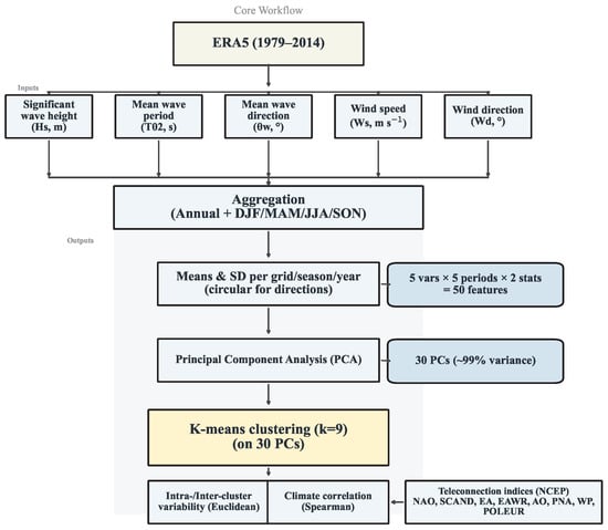
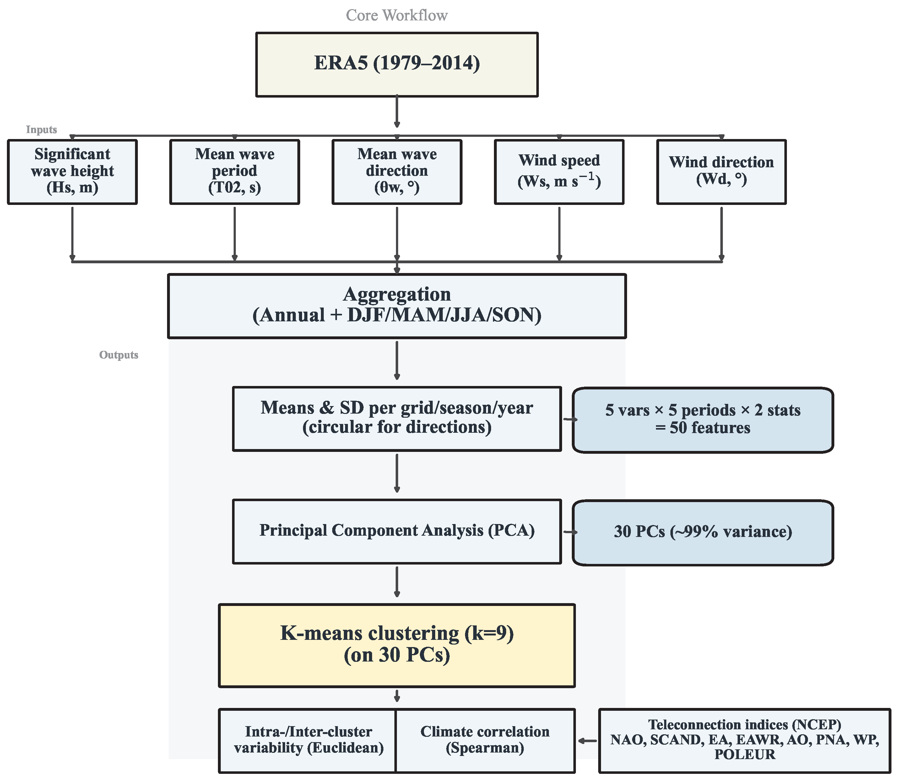
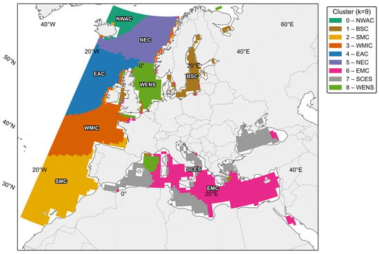
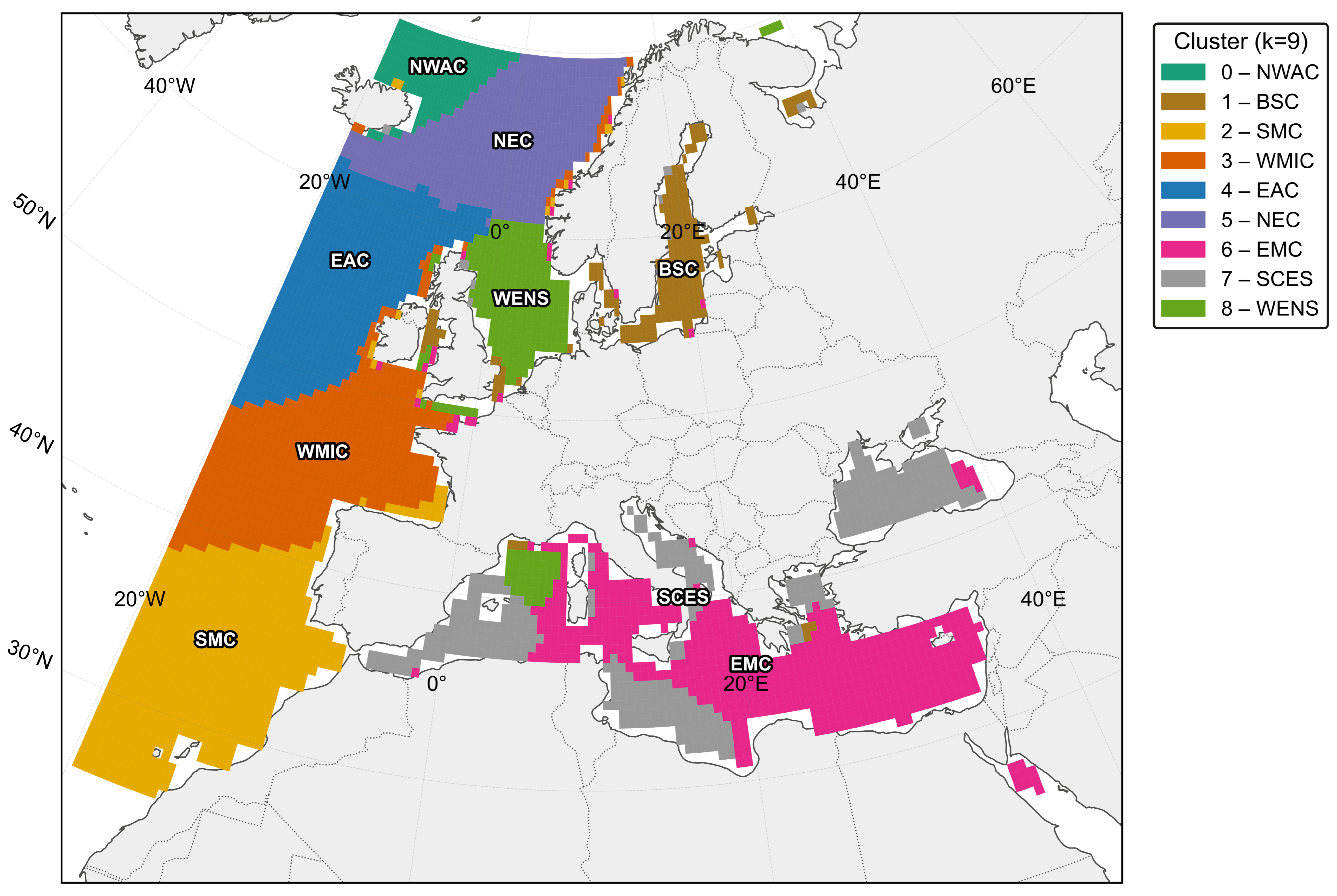
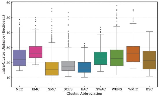
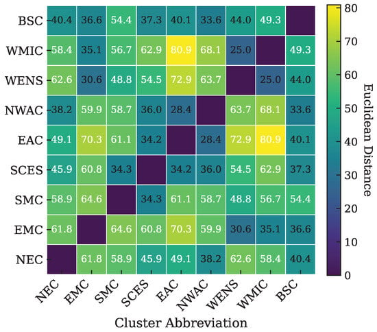
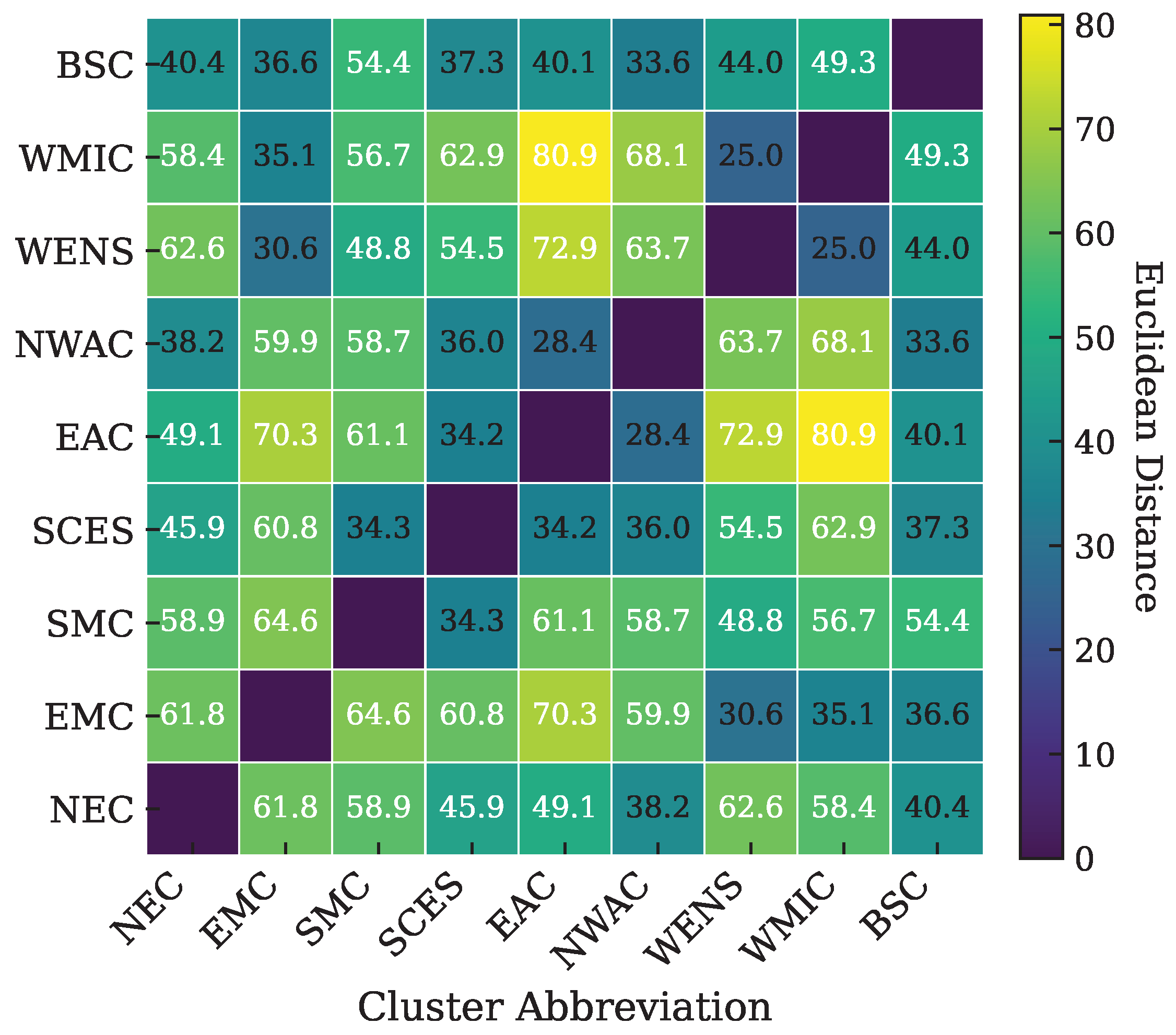
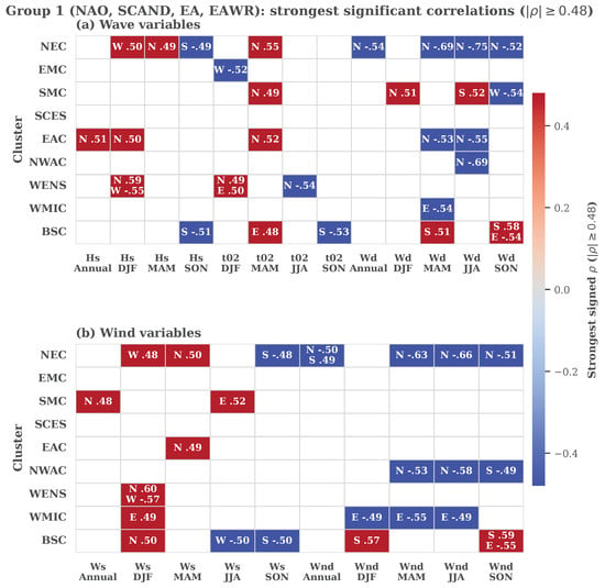
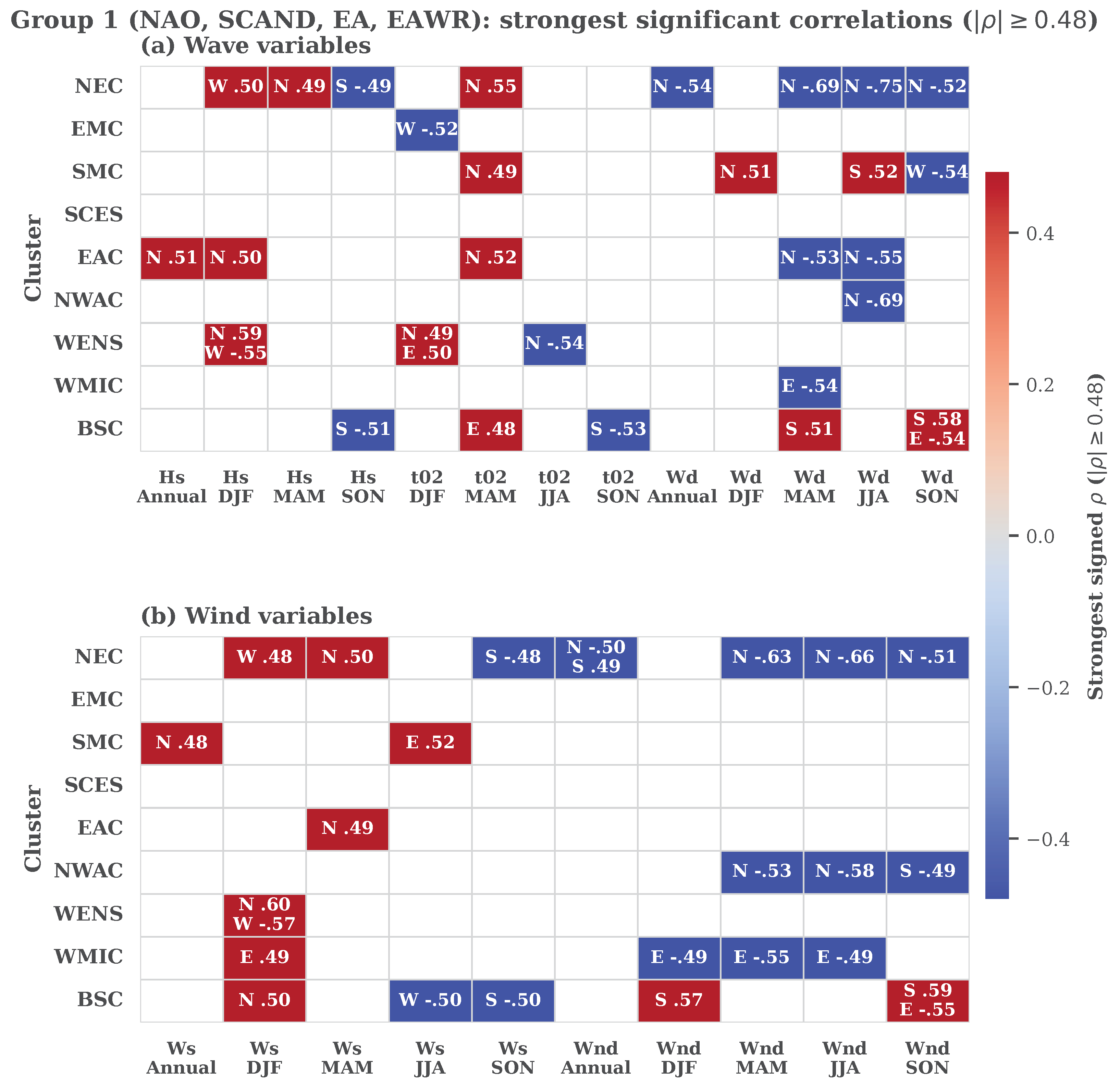
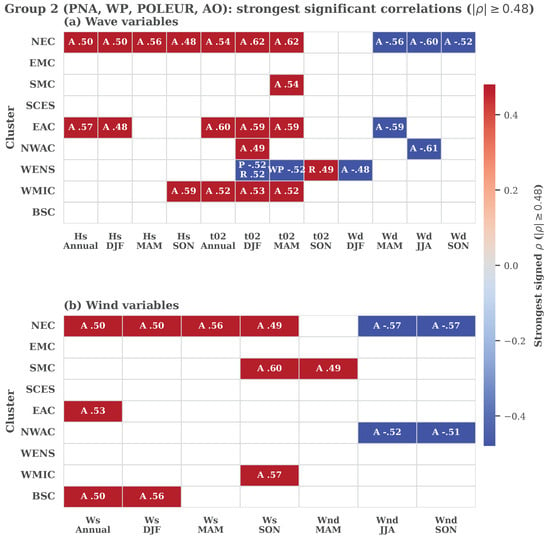
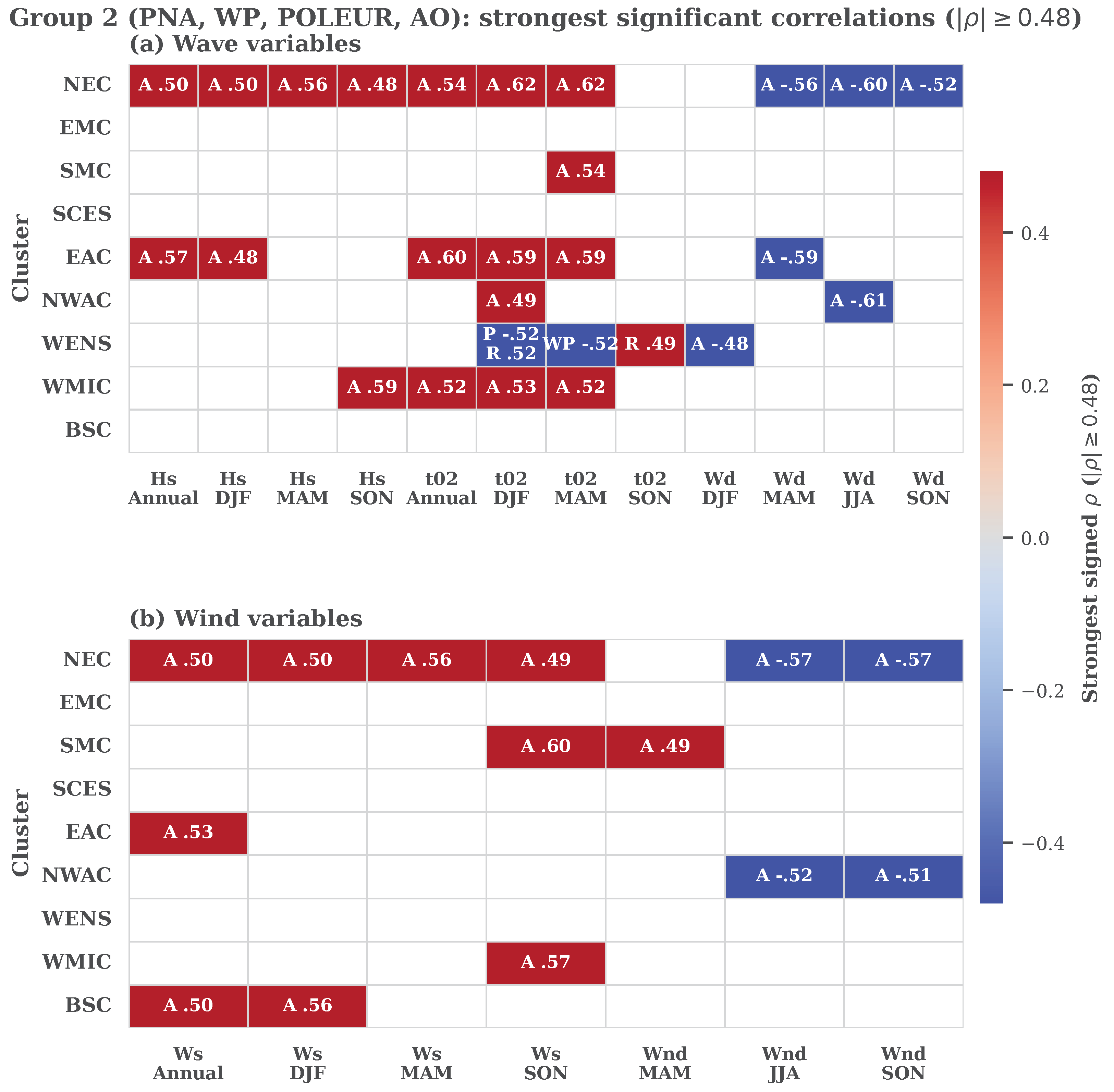

Disclaimer/Publisher’s Note: The statements, opinions and data contained in all publications are solely those of the individual author(s) and contributor(s) and not of MDPI and/or the editor(s). MDPI and/or the editor(s) disclaim responsibility for any injury to people or property resulting from any ideas, methods, instructions or products referred to in the content. |
© 2026 by the authors. Licensee MDPI, Basel, Switzerland. This article is an open access article distributed under the terms and conditions of the Creative Commons Attribution (CC BY) license.