Field Evaluation of CALINE4-Based Carbon Monoxide Dispersion Modeling at a Signalized Intersection in Ulaanbaatar, Mongolia

Abstract

Urban intersections are important hot spots of traffic–related air pollution, particularly in places where signal delays and idling increase vehicle emissions. This study evaluates near–road carbon monoxide (CO) concentrations at a signalized four–leg intersection in Ulaanbaatar, Mongolia, by combining field measurements with CALINE4 dispersion modeling. CO concentrations were measured at four receptor locations during two observation periods, 9:00–10:00 and 15:00–16:00. Hourly traffic volume, fleet composition, microclimatic conditions, and receptor geometry were used as model inputs. A fleet-weighted CO emission factor of 12.5 g veh⁻¹ mile⁻¹, adjusted for vehicle age and local stop-and–go traffic conditions, was applied as the base case, while 11.5 and 13.5 g veh⁻¹ mile⁻¹ were tested as sensitivity scenarios. The base case CALINE4 results reproduced the measured spatial pattern reasonably well, with overall performance indicators of r² = 0.759, FB = −0.006, NMSE = 0.010, RMSE = 0.400 ppm, and MAE = 0.325 ppm. Sensitivity analysis showed that higher emission factors increased predicted CO concentrations, although differences among scenarios were limited. The results suggest that the MOVES–CALINE4 modeling chain is suitable for preliminary screening level CO hot–spot assessment at congested intersections in Ulaanbaatar.

1. Introduction

Urban air pollution has become one of the major global environmental and public health challenges. In particular, pollutant concentrations in heavily trafficked road corridors frequently exceed permissible air quality standards. Previous studies have shown that long–term exposure to traffic–related air pollution is associated with respiratory diseases, cardiovascular disorders, and increased mortality risk [1]. In addition, air pollution is an important contributor to childhood respiratory diseases, particularly in low and middle–income countries in Asia [2]. Among the pollutants emitted by motor vehicles, carbon monoxide (CO) poses a significant health risk because it binds strongly to hemoglobin and reduces the oxygen–carrying capacity of the blood. Elevated concentrations of CO and other related pollutants near roads in heavily trafficked urban areas increase health risks for pedestrians and nearby residents [3].

Ulaanbaatar, the capital and administrative center of Mongolia, has a population of approximately 1.6–1.7 million and covers an area of about 4704.4 km². The city has experienced rapid urbanization and motorization over recent decades. Approximately 56% of all registered vehicles in Mongolia are concentrated in Ulaanbaatar, and motorized vehicles account for 97.7% of daily urban traffic. These conditions make congested signalized intersections in Ulaanbaatar suitable environments for assessing the—dispersion patterns of CO and other hazardous traffic–related pollutants.

The geographical setting of Ulaanbaatar, combined with its arid continental climate, promotes strong temperature inversions during winter and transitional seasons. Stable atmospheric conditions and low wind speeds restrict pollutant dispersion. The city also experiences a low atmospheric mixing layer height, which further enhances pollutant accumulation [4]. Rapid growth in vehicle ownership and persistent traffic congestion also contribute to elevated near–road CO concentrations [5]. Signalized intersections are often local air pollution hot-spots because they are characterized by vehicle idling, deceleration, long queues, and concentrated traffic flows. These operating conditions reduce fuel combustion efficiency and increase CO emissions [6]. Road geometry, transport infrastructure, land use patterns, and surrounding development also influence the dispersion of traffic–related pollutants [7].

Advanced dispersion models, including C–LINE, OSPM, ADMS–Urban, RLINE/AERMOD, OML–Highway, and Polyphemus, are widely used to evaluate pollutant concentrations near–roads. In the present study, CALINE4, which is based on Gaussian line–source theory, was selected. CALINE4 was chosen because it is suitable for the project level analysis of CO concentrations at specific monitoring locations and can be applied as a screening–level tool with relatively simple input requirements for intersection environments. Previous research has also shown that the integrated MOBILE6.2–CALINE4 framework can estimate near–road CO concentrations with reasonable accuracy [8]. Studies conducted in Indian cities reported that CALINE4 performed acceptably near intersections and under relatively flat terrain conditions [9,10]. However, model accuracy is highly dependent on wind conditions, traffic volume, emission factors, roadway geometry, and terrain complexity [9,11].

The performance of CALINE4 also varies according to pollutant type and study environment. In Detroit, USA, the model reproduced CO concentrations reasonably well but underestimated PM_2.5 concentrations [12]. In Himachal Pradesh, India, the model performed better in flat terrain than in mountainous areas [13]. Studies conducted in Beijing and Guangzhou concluded that the MOBILE6.2CALINE4 framework was suitable for estimating PM₁₀ concentrations near roads and intersections [14]. At a heavily trafficked intersection in Bangalore, modeled PM_2.5 concentrations showed acceptable agreement with field measurements [10]. Sensitivity analyses have identified traffic volume, emission factors, wind speed, and wind direction as the main parameters affecting CALINE4 predictions [15]. Nevertheless, unsatisfactory model performance has also been reported under certain high–traffic conditions [11]. Integrated approaches combining MOVES–Matrix with CALINE4 or AERMOD have improved computational efficiency while maintaining reliable results [16]. CALINE4 has also been successfully applied to studies of unsignalized intersections [17] and pedestrian exposure, where pollutant concentrations were found to decrease with increasing receptor height [18]. These findings indicate that CALINE4 is an efficient tool for the preliminary assessment of near–road CO and particulate matter concentrations. However, in areas characterized by complex terrain, variable meteorological conditions, traffic congestion, and uncertainty in emission factors, model outputs should be validated against local measurements.

Several studies have previously applied CALINE–type models to assess microscale carbon monoxide (CO) concentrations around roadway intersections. Abdul–Wahab applied the CAL3QHC model to estimate CO concentrations near a roadway intersection in Muscat, Oman [19], while Tippichai et al. used CAL3QHC to predict CO concentrations at signalized intersections in Khon Kaen, Thailand [20]. Subsequent studies also examined CO emission modeling at signalized intersections using CAL3QHC; for example, Kho et al. applied the model in Kuching, Malaysia [21], and Ritner et al. used a MOVES–CAL3QHC modeling framework that accounted for emissions during acceleration and deceleration phases [22]. However, localized applications that integrate field measurements, vehicle fleet composition, receptor geometry, meteorological input data, and emission factor estimation remain limited in the Mongolian context.

Therefore, the objective of this study is to evaluate CO concentrations near a heavily trafficked signalized four–leg intersection in Ulaanbaatar by integrating on–site measurements with CALINE4 dispersion modeling. The analysis combines traffic volume, vehicle fleet composition, micrometeorological conditions, roadway geometry, receptor locations, and emission factor estimation to compare measured and modeled CO concentrations. The findings are expected to clarify the applicability and limitations of CALINE4 under the specific traffic, meteorological, and topographical conditions of Ulaanbaatar. In addition, the study provides a scientific basis for improving traffic emission assessment and localized air quality management.

2. Methodology

In this study, a signalized four-leg intersection with high traffic demand in Ulaanbaatar City was selected, and the dispersion of CO emitted from road traffic was evaluated using a combination of field measurements and mathematical modeling. The methodological framework consists of five main stages: description of the study area, traffic survey, microclimatic measurements, emission factor estimation, and CALINE4 dispersion modeling framework.

CALINE4 was selected because this study aimed to provide an initial assessment of CO hot–spots at a signalized intersection using data collected during a relatively limited field campaign. The model was well suited to the available dataset, which included traffic volume, roadway geometry, receptor locations, estimated emission factors, wind speed, wind direction, and ambient temperature. It also offers a practical and transparent way to evaluate near–road pollutant dispersion when detailed meteorological and turbulence data are not available. For this reason, CALINE4 was used as a screening–level tool to examine spatial variations in CO concentrations and to compare measured and predicted values, rather than as a substitute for more advanced dispersion models requiring more comprehensive input data.

2.1. Study Area

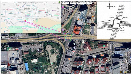
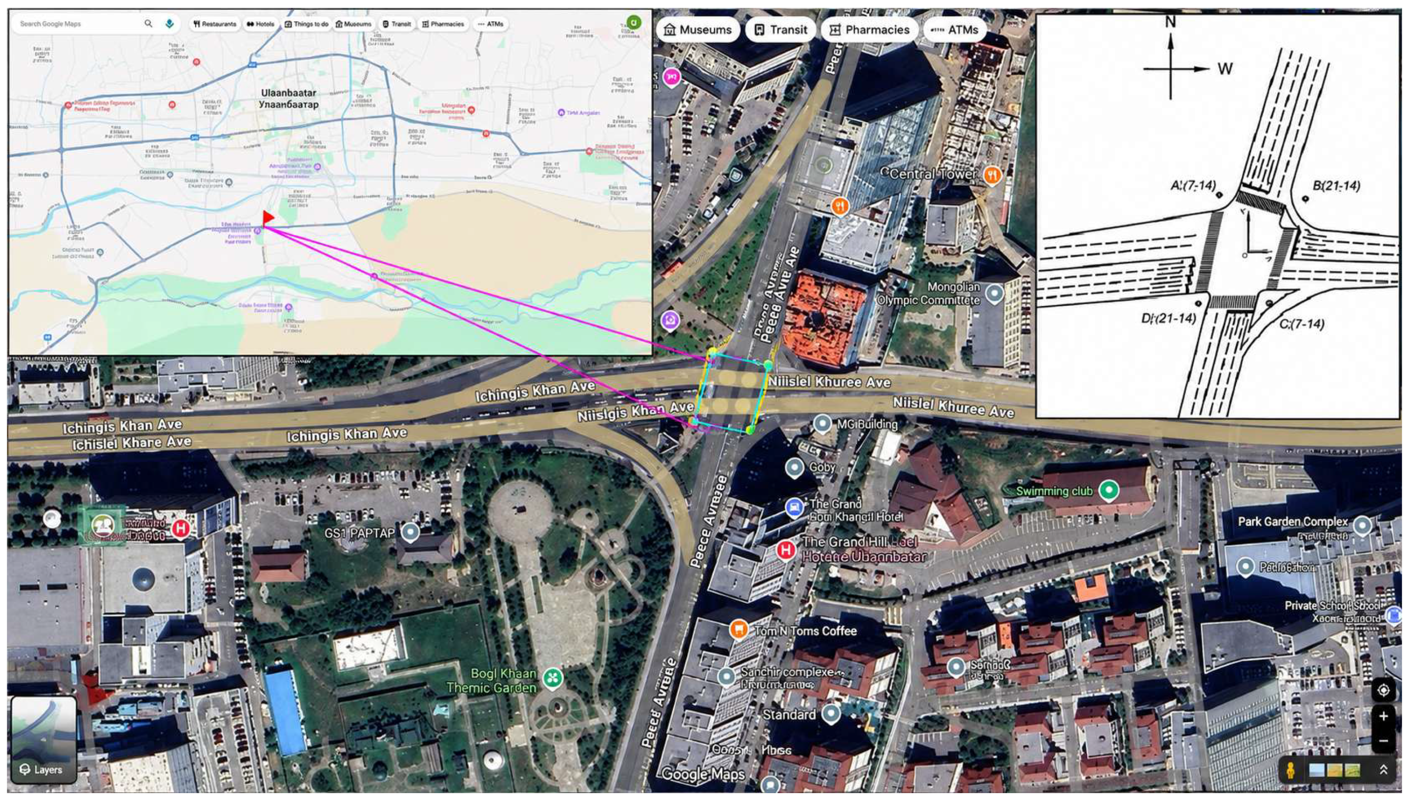
The study site was a signalized four–leg intersection located in the central area of Ulaanbaatar City characterized by heavy traffic volume. A circular zone with a radius of 200 m around the intersection was defined as the study and measurement domain. This zone included pedestrian crossings, residential areas, and commercial and service buildings. The layout of the intersection is illustrated in Figure 1.

Figure 1. Location of the study area, intersection layout, and measurement points, adapted and annotated from Google Maps using AutoCAD 2018. Map data/image © Google and respective data providers.

To accurately represent the spatial configuration of the intersection and the positioning of the monitoring equipment, four discrete receptor points (A, B, C, and D) were established. These points were situated at a uniform height along the vertical (Z) axis, strategically positioned at locations where pedestrian density is highest during signalized crossing intervals. The center of the intersection was defined as the coordinate origin (0,0). Two roadway links were represented as at–grade line sources: Link 1 for the east–west roadway and Link 2 for the south–north roadway. Four monitoring locations were represented as receptors A, B, C, and D, located around the intersection at a height of 1.2 m, which represents the approximate pedestrian breathing height.

Air quality measurements were conducted using an AQ–IQ Pod (USA, Colorado. College of Engineering and Applied Sciences), a portable low–cost air quality monitoring device developed by a research laboratory at the University of Colorado Boulder, USA. The device is designed to measure multiple air quality parameters, including CO, CO₂, PM₁, PM_2.5, and PM₁₀. Compared with conventional high-precision regulatory–grade monitoring instruments, the AQ–IQ Pod provides a lower–cost and more portable alternative for field–based air quality monitoring.

The geometric dimensions of the intersection are provided in Table 1, while the spatial coordinates of the receptor points are summarized in Table 2.

Table 1. CALINE4 geometric dimensions of the intersection.

Link	X1/(m)	Y1/(m)	X2/(m)	Y2/(m)
Link1	−200	0	200	0
Link2	0	−200	0	200

Table 2. Coordinates of measurement points.

Measurement Point	X/(m)	Y/(m)	Z/(m)
A	−7	14	1.2
B	21	14	1.2
C	7	−14	1.2
D	−21	−14	1.2

2.2. Traffic Survey

The field survey was carried out on 29 August 2024, a regular weekday in autumn. The date was chosen because there were no public holidays, major road closures, traffic restrictions, or unusual weather conditions that could have affected normal travel patterns. The traffic conditions observed during the survey were therefore considered representative of a typical weekday at the selected signalized intersection. Data were collected during both the morning and afternoon periods to capture changes in CO concentrations under different traffic and meteorological conditions. Traffic volumes and vehicle movements at the four–leg intersection were recorded using drone footage together with video recordings from fixed cameras.

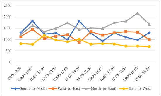
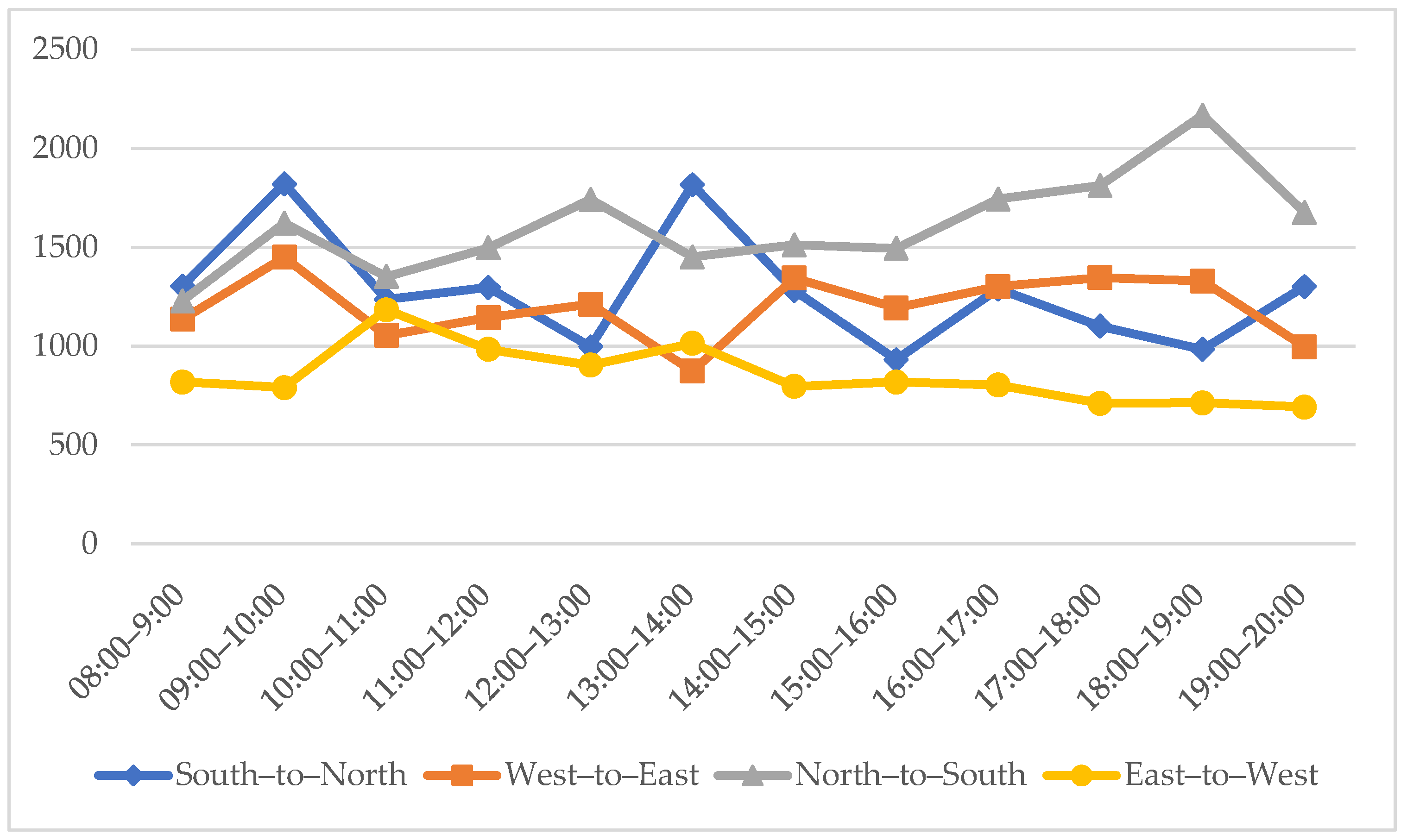
Figure 2 presents the hourly directional traffic volumes recorded from 08:00 to 20:00 for four movements: southnorth, west–to–east, north–to–south, and east–to–west. Traffic was unevenly distributed between the two principal roadway axes, with approximately 58% of the total traffic travelling along the north–to–south axis and 42% along the east–to–west axis.

Figure 2. Hourly directional traffic volumes at the intersection from 08:00 to 20:00 on 29 August 2024.

For the CALINE4 model, the four directional traffic streams were aggregated into two roadway links. Link 1 represents the east–to–west roadway and was calculated as the sum of the west–to–east and east–to–west traffic streams. Link 2 represents the north–to–south roadway and was calculated as the sum of the south–to–north and north–to–south streams. The highest total hourly traffic volume was recorded during 09:00–10:00, reaching 5689 vehicles per hour; therefore, this period was selected as the morning peak–hour base case. The 15:00–16:00 period, with a total volume of 4442 vehicles per hour, was also modeled to compare the predicted concentrations with the CO concentrations measured during the afternoon survey. The aggregated traffic volumes used as CALINE4 model inputs are summarized in Table 3.

Table 3. Traffic volumes aggregated by CALINE4 roadway link for the modeled periods.

Period	Link 1: East–to–West (veh/h)	Link 2: South–to–North (veh/h)	Total (veh/h)
9:00–10:00	2243	3446	5689
15:00–16:00	2014	2428	4442

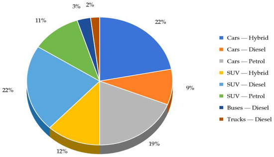
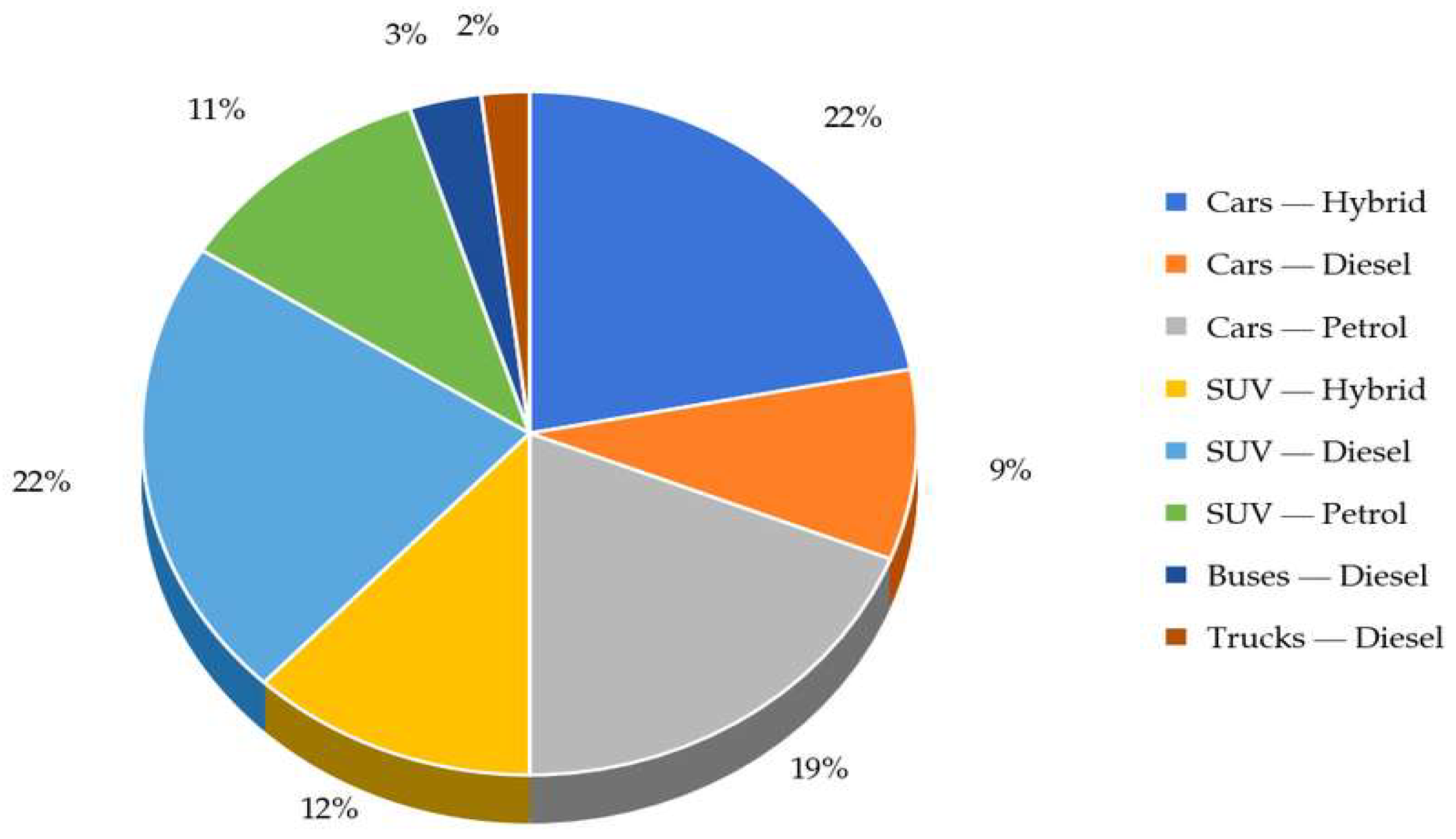
The vehicle fleet composition observed during the traffic survey is presented in Figure 3. The surveyed fleet included hybrid, diesel, and petrol passenger cars and SUV’s, as well as diesel–powered buses and trucks.

Figure 3. Composition of vehicle types observed at the intersection on 29 October 2024.

2.3. Meteorological Measurements During the Field Campaign

During the CO measurement campaign at the signalized intersection in Ulaanbaatar, local field meteorological parameters were recorded at approximately pedestrian breathing height using a handheld anemometer (China, Electronic wind speed meter tester, model HT625B). In accordance with the World Meteorological Organization (WMO) Guide to Instruments and Methods of Observation, wind speed and air temperature were considered essential field observation variables for interpreting near–road pollutant dispersion [23]. The measured wind speed, wind direction, and ambient temperature represent short–term meteorological conditions during the field campaign and were used as input parameters for CALINE4. They should not be interpreted as a long–term microclimatic characterization of the study area.

Wind speed and ambient temperature were measured using a handheld anemometer, while wind direction was determined separately using compass–based field observations and expressed according to the meteorological convention. For example, 315° indicates wind originating from the northwest.

The micro–meteorological parameters used for CALINE4 input and wind–rose visualization are summarized in Table 4. Hourly average values were used as the direct CALINE4 input, while the minimum and maximum values were retained to describe the observed range of field conditions during the two measurement periods.

Table 4. Completed meteorological data used for CALINE4 input and reconstructed wind–rose visualization.

Parameter	09:00–10:00 Avg	09:00–10:00 Min	09:00–10:00 Max	15:00–16:00 Avg	15:00–16:00 Min	15:00–16:00 Max
Wind speed/(m/s)	1.2	0	3.5	1.8	0	4
Wind direction/(deg)	315	285	345	295	255	335
Wind direction std.dev./(deg)	15	-	-	20	-	-
Ambient temperature/(°C)	16	14	17	19	17	20

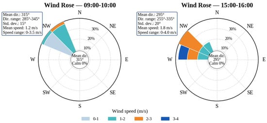
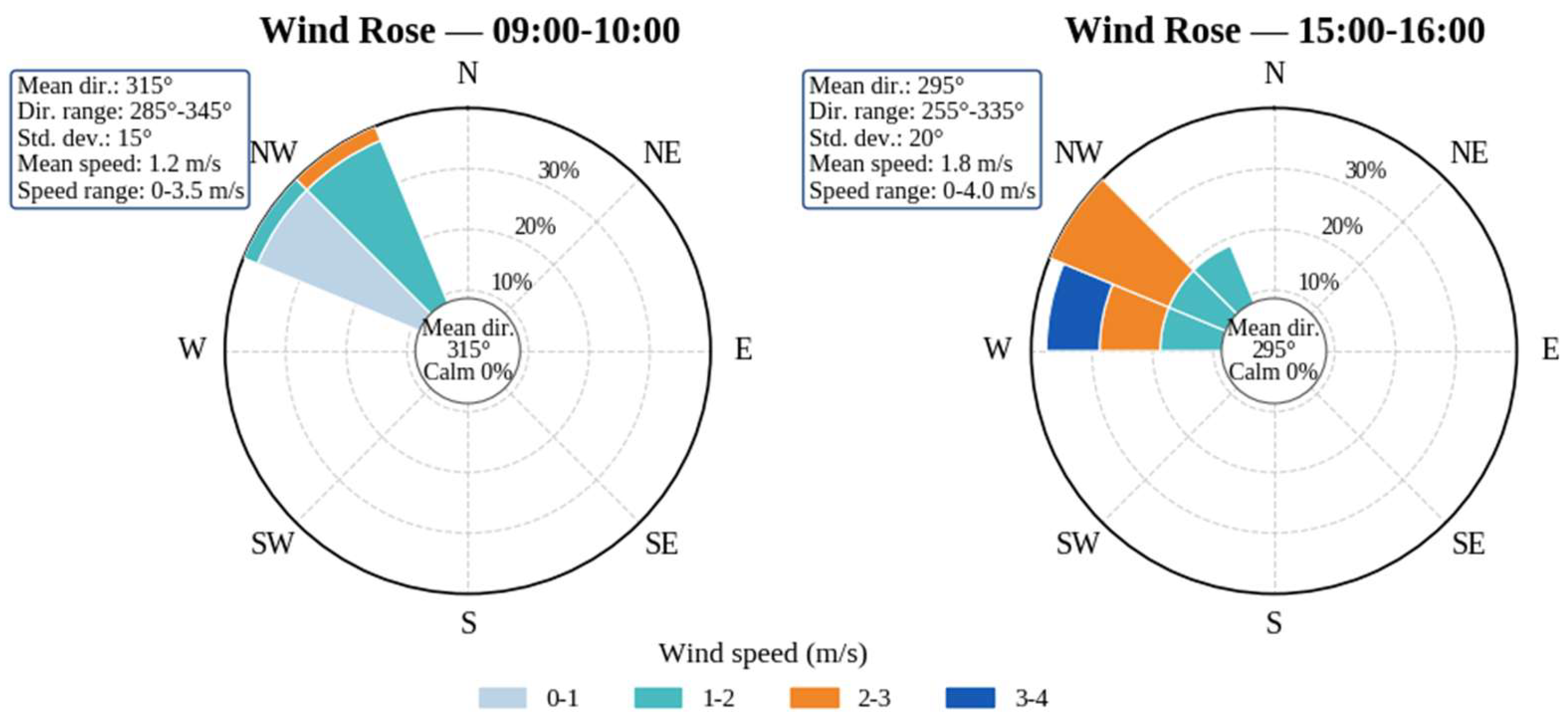
Figure 4 presents the wind–rose diagrams for the two modeled periods, showing the distribution of wind direction and wind speed. During 09:00–10:00, the average wind speed was 1.2 m/s, with an observed range of 0–3.5 m/s, and the dominant wind direction was 315°. During 15:00–16:00, the average wind speed increased to 1.8 m/s, with a range of 0–4.0 m/s, while the dominant wind direction shifted to 295°. The ambient temperature ranged from 14–17 °C during the morning period and from 17–20 °C during the afternoon period.

Figure 4. Wind–rose diagrams showing wind direction and wind speed distributions during the morning (09:00–10:00) and afternoon (15:00–16:00) modeling periods.

Because continuous high–frequency wind direction measurements were unavailable, the wind rose was reconstructed from field observations and aggregated meteorological data. A synthetic 5-min interval series was generated solely for visualization and was not treated as an independent set of raw observations. The reconstruction preserved the observed hourly mean wind speed, wind speed range, dominant wind direction, directional variability, and temperature range.

Wind direction standard deviation was included to represent directional variability during the two measurement periods. In CALINE4–related CO screening applications, wind direction and wind direction standard deviation are important meteorological inputs; the Sacramento Metropolitan Air Quality Management District CO modeling guidance notes that a wind direction standard deviation may be specified and recommends 5° for worst–case screening conditions [2]. In this study, standard deviations of 15° for 09:00–10:00 and 20° for 15:00–16:00 were used to represent moderate directional variability observed during the field campaign.

Accordingly, the reconstructed wind rose should be interpreted as a supporting visualization of the meteorological conditions used in the dispersion–modeling framework, whereas the CALINE4 simulation itself was parameterized using the observed hourly average meteorological values shown in Table 4.

2.4. Emission Factor Estimation

The emission factors (EFs) for CO emitted from vehicles were selected based on internationally recognized models widely used in previous studies. Considering vehicle fleet composition and traffic conditions, the weighted emission factor (WEF) was calculated.

An EF represents the amount of pollutant emitted per unit distance traveled (g/km) by a specific vehicle type. EF values depend on multiple factors, including vehicle type, fuel type, vehicle age, maintenance condition, engine performance, and meteorological conditions [24,25,26].

In Mongolia, vehicles are imported, and a nationally developed EF database (EFDB) has not yet been established. Consequently, international empirical models are commonly used to estimate vehicle emissions. As noted by Bayasgalan and Matsumoto [27], EF standards based on vehicles operating in Mongolia have not yet been fully developed, although related research began in 2014.

The vehicular fleet in Mongolia exhibits a heavily skewed age distribution, with approximately 80% of vehicles exceeding 10 years of age, while those aged 0–3, 4–6, and 7–9 years account for only 6%, 4%, and 10%, respectively [28]. Mongolia’s vehicle fleet is characterized by a high share of old vehicles, which contributes to elevated exhaust emissions and urban air quality deterioration. Therefore, the emission assessment in this study was supported by national vehicle statistics and Mongolia’s National Inventory Report submitted to the UNFCCC [29]. Furthermore, chronic traffic congestion in Ulaanbaatar, characterized by sustained low operational speeds (10–20 km/h) and extensive engine idling, significantly exacerbates emission factors (EFs).

Given these localized complexities, CO values were estimated using the USEPA MOVES (Motor Vehicle Emission Simulator) framework [30]. The MOVES model was selected for its high–fidelity capacity to integrate multi–dimensional variables, including vehicular age bins, fuel specifications, transient driving cycles, and ambient meteorological parameters [31]. Furthermore, the MOVES model is widely recognized as a state–of–the–art emission modeling tool that improves the accuracy of emission factor estimation at national and regional scales by incorporating driving patterns and vehicle operating conditions [32].

The CO emission factor used as an input to the CALINE4 dispersion model was estimated as a literature–based proxy emission factor rather than a direct MOVES simulation output. This approach was adopted because the MOVES model was not executed for the study site. Nevertheless, the method retains consistency with MOVES–based emission rate concepts by using published vehicle–type–specific emission factors and then adapting them to the observed fleet composition at the intersection. CALINE4 was selected for projectlevel CO hot–spot analysis, which is consistent with Caltrans’ guidance that identifies CALINE4 as applicable to CO hot–spot analysis near roadways [33].

The baseline CO emission factors were obtained from the Bureau of Transportation Statistics (BTS) Table 4-43, which reports estimated national average vehicle emission rates in grams per mile. The current BTS Table 4-43 is generated using EPA MOVES4 and states that the emission factors are averages based on national age distributions, vehicle activity, operating modes, speeds, temperature conditions, inspection/maintenance assumptions, and average fuel properties. The table also specifies that gasoline–electric hybrid vehicles are represented within the gasoline vehicle category [34]. For the numerical proxy calculation, the archived BTS Table 4-43 values for 2010 were used because the relevant CO values are explicitly available by vehicle type and fuel type. The selected CO values were as follows: gasoline lightduty vehicle = 8.73 g veh⁻¹ mile⁻¹, gasoline light–duty truck = 11.02 g veh⁻¹ mile⁻¹, diesel light–duty vehicle = 0.90 g veh⁻¹ mile⁻¹, diesel light–duty truck = 0.76 g veh⁻¹ mile⁻¹, and diesel heavy–duty vehicle = 1.75 g veh⁻¹ mile⁻¹ [35].

As summarized in Table 5, the observed vehicle composition at the intersection was mapped to the corresponding BTS vehicle classes, resulting in a fleet–weighted emission factor of 6.41 g veh⁻¹ mile⁻¹. Cars–Hybrid and Cars–Petrol were assigned to gasoline light–duty vehicles, Cars–Diesel to diesel light–duty vehicles, SUV–Hybrid and SUV–Petrol to gasoline light–duty trucks, SUV–Diesel to diesel light–duty trucks, and Buses–Diesel and Trucks–Diesel to diesel heavy–duty vehicles.

Table 5. Emission factors (EF) calculated using the MOVES model.

Vehicle Type	Observed Share (%)	Assigned Emission Class	EFᵢ/(g veh−1 mile−1)	Weighted EF (g veh−1 mile−1)
Cars—Hybrid	22	Gasoline light–duty vehicle	8.73	1.92
Cars—Diesel	9	Diesel light–dutyvehicle	0.90	0.08
Cars—Petrol	19	Gasoline light–dutyvehicle	8.73	1.63
SUV—Hybrid	12	Gasoline light–dutytruck	11.02	1.31
SUV—Diesel	22	Diesel light–dutytruck	0.76	0.17
SUV—Petrol	11	Gasoline light–dutytruck	11.02	1.21
Bus—Diesel	3	Diesel heavy–duty vehicle	1.75	0.06
Truck—Diesel	2	Diesel heavy–duty vehicle	1.75	0.03
Total	100	-	-	6.41

However, this baseline value represents U.S. national average conditions and cannot fully represent the Mongolian vehicle fleet, which is characterized by a high proportion of old vehicles. National road safety statistics indicate that a dominant share of registered vehicles in Mongolia has been used for 10 years or more [36]. Therefore, an age–related deterioration factor and a traffic–condition factor were applied to account for the older fleet and low–speed stop–and–go operation at the intersection. The adjusted CO emission factor was calculated as:

$${\mathrm{E}\mathrm{F}}_{(\mathrm{C}\mathrm{O},\mathrm{a}\mathrm{d}\mathrm{j})}={\mathrm{E}\mathrm{F}}_{(\mathrm{b}\mathrm{a}\mathrm{s}\mathrm{e},\mathrm{f}\mathrm{l}\mathrm{e}\mathrm{e}\mathrm{t})}\times {\mathrm{K}}_{\left(\mathrm{a}\mathrm{g}\mathrm{e}\right)}\times {\mathrm{K}}_{\left(\mathrm{t}\mathrm{r}\mathrm{a}\mathrm{f}\mathrm{f}\mathrm{i}\mathrm{c}\right)}$$

(1)

${\mathrm{K}}_{\left(\mathrm{a}\mathrm{g}\mathrm{e}\right)}$ is the vehicular age correction factor.

${\mathrm{K}}_{\left(\mathrm{t}\mathrm{r}\mathrm{a}\mathrm{f}\mathrm{f}\mathrm{i}\mathrm{c}\right)}$ is the traffic operating condition adjustment factor.

In this study, ${\mathrm{K}}_{\left(\mathrm{a}\mathrm{g}\mathrm{e}\right)}=1.5$ was used to account for emission deterioration associated with the high share of old vehicles in the local fleet, while ${\mathrm{K}}_{\left(\mathrm{t}\mathrm{r}\mathrm{a}\mathrm{f}\mathrm{f}\mathrm{i}\mathrm{c}\right)}=1.3$ was used to represent low–speed stop–and–go operation at the signalized intersection [37]. These coefficients were applied as engineering adjustment factors to localize the literature–based baseline emission factor to the study context. Because they were not derived from local dynamometer measurements or direct MOVES simulations, they represent a source of uncertainty. Therefore, sensitivity scenarios were applied to evaluate the influence of the assumed emission factor on predicted CO concentrations. Thus:

$${\mathrm{E}\mathrm{F}}_{(\mathrm{C}\mathrm{O},\mathrm{a}\mathrm{d}\mathrm{j})}=6.41\times 1.5\times 1.3=12.5·g·{\mathrm{veh}}^{-1}{\mathrm{mile}}^{-1}$$

Accordingly, the CO emission factor used in the CALINE4 model was set to 12.5 g veh⁻¹ mile⁻¹. Since this value is not a direct MOVES output, it should be interpreted as a literature–based proxy emission factor. To assess the uncertainty in this assumption, sensitivity analyses were performed using 11.5 and 12.5 g veh⁻¹ mile⁻¹.

2.5. CALINE4 Model Setup and Dispersion Modeling

The CALINE4 dispersion model was used to estimate near–road carbon monoxide (CO) concentrations at the selected signalized four–leg intersection. CALINE4 is a steady-state Gaussian line–source model developed for roadway air quality assessment and describes pollutant dispersion using Gaussian diffusion theory together with a roadway mixing zone concept [38,39].

Although CALINE4 can be applied to several transport–related pollutants, the present application focuses on CO because it is a typical pollutant for intersection–level hot–spot analysis. Caltrans notes that CALINE4 is currently applied for CO hot–spot analysis in project–level air quality studies [40]. Accordingly, the input dataset was organized to represent the dominant roadway links, receptor locations, selected hourly traffic counts, emission–factor assumptions, and micro–meteorological conditions recorded during the field campaign.

The main input parameters used in the CALINE4 simulation are summarized in Table 6. Since site–specific mixing height measurements were not available during the field campaign, a representative mixing height of 500 m was assumed for the screening–level CALINE4 simulation. This value was used only as a screening–level modeling assumption and should not be interpreted as a measured boundary layer height. This assumption introduces uncertainty, particularly under stable atmospheric conditions.

Table 6. Input parameters used in the CALINE4 dispersion model.

No.	Parameter	Value/Unit	Source
1	Traffic data	1-h traffic volume (veh h−1)	Camera and manual count
2	Weighted emission factor	12.5 g veh−1 mile−1	Calculated in this study
3	Emission factor basis	BTS Table 4-43/EPA MOVES4	Literature–based fleet–weighted CO emission factor using MOVES/BTS–derived values
4	Terrain type	Urban	Field observation
5	Mixing zone width	30 m	Field measurement
6	Roadway geometry	Two at-grade links	Field layout/coordinate system
7	Receptor points	A, B, C, D at 1.2 m	Field measurement locations
8	Wind speed	m/s	On-site field measurement using handheld digital anemometer
9	Wind direction		Compass–based field observation using meteorological convention
10	Wind direction std. dev.		Estimated from repeated directional observations/reconstructed series
11	Ambient temperature	°C	On-site field measurement using handheld digital anemometer
12	Mixing height	500 m	Assumed for screening–level simulation; site–specific data were not available future studies
13	Dispersion model		CALINE4 Gaussian line–source dispersion model

The CO emission factor was entered in g veh⁻¹ mile⁻¹, which is consistent with roadway dispersion modeling practice where emission rates are commonly specified in grams per mile for the corresponding vehicle category, speed, and operating condition [41]. The final input structure combined direct field observations, study–specific calculations, and screening–level assumptions. Traffic volume, roadway geometry, receptor coordinates, terrain type, and mixing zone width were obtained from field observation and measurement. The fleet–weighted CO emission factor was calculated in this study using literature–based MOVES/BTS–derived emission factors and local adjustment coefficients. Meteorological variables were obtained from on–site measurements and reconstructed directional statistics, while the mixing height was assumed for the screening–level modeling framework.

3. Results

Measured and CALINE4–predicted CO concentrations were compared for two observation periods, 9:00–10:00 and 15:00–16:00, at the four receptor locations (A–D) established around the signalized intersection. The base modeling case used a CO emission factor of EF = 12.5 g veh⁻¹ mile⁻¹, which was derived from the fleet–weighted emission factor estimation procedure and adjusted to reflect vehicle age and local stop–and–go traffic conditions. In addition, EF = 11.5 and 13.5 g veh⁻¹ mile⁻¹ were applied as lower and upper sensitivity scenarios to examine how uncertainty in the emission factor affects the predicted CO concentrations.

As shown in Table 7, the modeled concentrations generally follow the measured spatial pattern across the receptor points. Because only four receptor points were used, the results should be interpreted as local concentration differences among selected pedestrian–level receptor locations rather than as a complete spatial distribution of CO around the intersection. Accordingly, the revised analysis focuses on receptor–level measured–versus–modeled differences rather than spatial interpolation.

Table 7. Measured and CALINE4–predicted CO concentrations/(ppm) under different emission factor scenarios/(g veh⁻¹ mile⁻¹).

Time	Location	Measured CO/(ppm)	CALINE4 CO, EF = 11.5 veh−1 mile−1/(ppm)	CALINE4 CO, EF = 12.5 veh−1 mile−1/(ppm)	CALINE4 CO, EF = 13.5 veh−1 mile−1/(ppm)
9:00–10:00	A	3.6	3.4	3.5	3.5
	B	5.1	4.2	4.3	4.5
	C	5.4	5.1	5.3	5.5
	D	4.2	4.0	4.0	4.1
15:00–16:00	A	2.9	3.3	3.4	3.4
	B	3.7	3.7	3.8	3.9
	C	4.1	4.4	4.5	4.7
	D	3.5	3.8	3.9	4.0

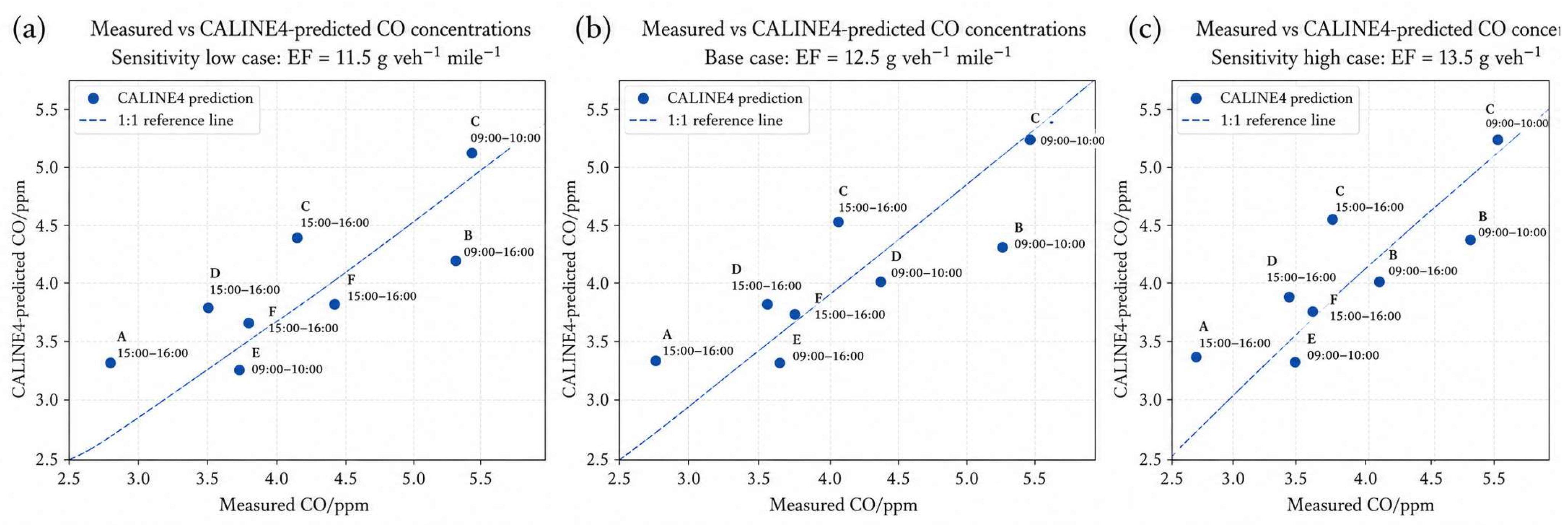
During the morning period, the highest measured CO concentration was recorded at receptor C (5.4 ppm), and the corresponding base case CALINE4 prediction was 5.3 ppm. In the afternoon period, the measured CO concentrations were lower, ranging from 2.9 to 4.1 ppm, while the base case predictions ranged from 3.4 to 4.5 ppm. These results indicate that CALINE4 reproduced the overall magnitude of near–road CO concentrations reasonably well, although some receptor-specific deviations remained.

Figure 5 presents measured-versus-predicted scatter plots for the complete dataset under three CO emission factor scenarios: EF = 11.5, 12.5, and 13.5 g veh⁻¹ mile⁻¹. Each panel includes eight paired observations obtained from four receptor locations during the 09:00–10:00 and 15:00–16:00 monitoring periods. The dashed 1:1 reference lines indicate perfect agreement between the measured and CALINE4-predicted concentrations. These scatter plots, together with the tabulated concentration values and statistical performance indicators, provide the basis for evaluating model agreement, receptor-specific deviations, and sensitivity to the selected emission factor.

Figure 5. Measured–versus–predicted scatter plots for the complete dataset under three emission–factor scenarios: (a) sensitivity low case, EF = 11.5 g veh⁻¹ mile⁻¹; (b) base case, EF = 12.5 g veh⁻¹ mile⁻¹; and (c) sensitivity high case, EF = 13.5 g veh⁻¹ mile⁻¹. The dashed lines represent perfect 1:1 agreement between measured and predicted CO concentrations. Labels indicate the receptor locations and monitoring periods.

3.1. Statistical Performance of the Base Case

The statistical performance indicators for the CALINE4 base case (EF = 12.5 g veh⁻¹ mile⁻¹) are summarized in Table 8. For the base case (EF = 12.5 g veh⁻¹ mile⁻¹), the overall statistical indicators were r² = 0.759, FB = −0.006, NMSE = 0.010, RMSE = 0.400 ppm, and MAE = 0.325 ppm. The normalized mean square error (NMSE) was calculated using the air quality model performance formulation: $NMSE=mean\left[\right(Cp-Co{)}^2]/(meanCp\times meanCo)$, where Cp and Co denote predicted and observed CO concentrations, respectively. To avoid ambiguity in the interpretation of relative error, normalized MAE was additionally calculated as MAE divided by the mean observed concentration. Thus, NMSE and normalized MAE were treated as distinct performance indicators. The near-zero FB indicates that CALINE4 produced almost no systematic bias across the full dataset, while the low NMSE suggests limited normalized scatter between measured and predicted concentrations.

Table 8. Statistical performance indicators for the CALINE4 base case (EF = 12.5 g veh⁻¹ mile⁻¹).

Case	Mean Measured/(ppm)	Mean CALINE4/(ppm)	r2	FB	NMSE	RMSE/(ppm)	MAE/(ppm)
9:00–10:00	4.575	4.275	0.834	0.068	0.009	0.418	0.300
15:00–16:00	3.550	3.900	0.881	−0.094	0.010	0.381	0.350
Overall	4.062	4.088	0.759	−0.006	0.010	0.400	0.325

3.2. Sensitivity Analysis Results

Table 9 summarizes the sensitivity analysis conducted using three CO emission factor scenarios. As the emission factor increased, the mean predicted CO concentration also increased, while FB shifted from slight underprediction at 11.5 g veh⁻¹ mile⁻¹ to slight overprediction at 13.5 g veh⁻¹ mile⁻¹. However, the overall differences among the scenarios were small, with RMSE values ranging from 0.400 to 0.406 ppm and MAE values from 0.325 to 0.338 ppm. The base case, EF = 12.5 g veh⁻¹ mile⁻¹, provided the closest overall agreement with the observations, producing a mean predicted concentration of 4.088 ppm compared with the measured mean of 4.062 ppm. It also yielded the lowest RMSE of 0.400 ppm, an MAE of 0.325 ppm, and an FB value close to zero, indicating minimal systematic bias. These error values correspond to approximately 9.8% and 8.0% of the mean measured concentration, respectively. Although the lower emission factor scenario produced a slightly higher $r^2$, the base case was retained because it provided the most balanced performance across the evaluation metrics and was derived from the fleet–weighted and traffic–adjusted emission factor estimation procedure rather than selected solely on the basis of statistical fit.

Table 9. Sensitivity analysis of CALINE4 prediction performance under different CO emission factors.

Case	Mean Measured/(ppm)	Mean CALINE4/(ppm)	r2	FB	NMSE	RMSE/(ppm)	MAE/(ppm)
EF = 11.5 g veh−1 mile−1 (Sensitivity low)	4.062	3.987	0.772	0.019	0.010	0.406	0.325
EF = 12.5 g veh−1 mile−1 (Base case)	4.062	4.088	0.759	−0.006	0.010	0.400	0.325
EF = 13.5 g veh−1 mile−1 (Sensitivity high)	4.062	4.200	0.771	−0.033	0.009	0.402	0.338

4. Discussion

The results indicate that the MOVES–CALINE4 modeling chain reproduced the general magnitude and spatial distribution of near–road CO concentrations at the signalized intersection. In the base case, the morning period showed strong agreement between the measured and predicted values (r² = 0.834, RMSE = 0.418 ppm, MAE = 0.300 ppm), while the afternoon period also showed a high linear association (r² = 0.881) with low absolute errors (RMSE = 0.381 ppm, MAE = 0.350 ppm). The overall statistics (r² = 0.759, FB = −0.006, NMSE = 0.010) suggest that the model captured the receptor–to–receptor variation with minimal systematic bias. The small negative FB indicates a slight overall overprediction, but its magnitude is sufficiently low to consider the bias negligible for screening–level interpretation.

The model performance observed in this study is consistent with previous applications of CALINE4 for near–road CO assessment. Validated CALINE4 for predicting carbon monoxide concentrations near urban roads and evaluated the model using statistical indicators such as correlation, fractional bias, and NMSE [42]. Similarly, Ellis et al. reported that CALINE4 can provide useful near–road concentration estimates, although its performance may be lower than more advanced roadway dispersion models under some conditions [43]. These findings support the interpretation that CALINE4 is appropriate for preliminary or screening–level evaluation when input data are limited but traffic, receptor, and meteorological parameters are carefully defined.

The sensitivity analysis also confirms that the emission factor is an important source of uncertainty in the modeling chain. Dhyani, R et al [15] showed that CALINE4 predictions are sensitive to traffic, emission, meteorological, and roadway parameters, including wind speed, wind direction, emission factor, traffic volume, and roadway width. In the present study, changing the CO emission factor from 11.5 to 13.5 g veh⁻¹ mile⁻¹ changed the mean predicted CO concentration from 3.987 to 4.200 ppm, while the RMSE changed only slightly. This indicates that, within the tested range, the selected emission factor affected the magnitude of predicted CO but did not substantially alter the overall spatial pattern.

Although the diesel vehicle categories showed relatively low CO emission factors in the fleet–weighted calculation, this should not be interpreted as evidence that diesel vehicles have a negligible air quality impact. Diesel engines are typically more relevant for particulate matter and nitrogen oxides emissions than for CO emissions. Therefore, the present CO–focused assessment should be complemented in future work by multi–pollutant modeling, particularly for PM_2.5, PM₁₀, and NOx.

Several limitations should be considered when interpreting the results. First, the line-source representation simplifies the complex acceleration, deceleration, idling, and queue formation processes that occur at a signalized intersection. Second, the limited number of receptor points is an important source of uncertainty. Four receptor locations are insufficient to characterize the full spatial distribution of CO around the intersection; therefore, the results should be interpreted only as local pedestrian–level concentration differences.

Third, local wind fields may be affected by surrounding buildings, street geometry, and short–term turbulence, which are not fully represented by hourly average meteorological inputs. In addition, site–specific mixing–height data were not available during the field campaign. Therefore, a representative mixing height was assumed for the screening–level CALINE4 simulation. This assumption may affect predicted concentrations, particularly under stable atmospheric conditions or thermal inversion events, which are common in Ulaanbaatar. Fourth, background CO concentration was not continuously monitored at a high temporal resolution. Finally, the emission factor was estimated using a literature based, fleet weighted proxy and local adjustment factors rather than a direct MOVES simulation using local vehicle operating modes.

As recommended by [44], air quality model performance should therefore be interpreted using multiple indicators rather than a single statistic. The present results should be regarded as a reasonable screeninglevel CO hot–spot assessment, which is consistent with Caltrans’ guidance identifying CALINE4 as applicable for project–level CO hot–spot analysis.

5. Conclusions

The statistical evaluation demonstrates that the CALINE4 base case with EF = 12.5 g veh⁻¹ mile⁻¹ provides a reasonable screening–level estimate of CO concentration at the signalized intersection. The overall performance indicators (r² = 0.759, FB = −0.006, NMSE = 0.010, RMSE = 0.400 ppm, and MAE = 0.325 ppm) indicate good spatial agreement, low normalized scatter, and negligible systematic bias. The model reproduced both morning and afternoon concentration patterns with relatively small errors, suggesting that the MOVES–CALINE4 modeling chain can be used as a practical preliminary tool for assessing traffic–related CO hot spots at congested urban intersections in Ulaanbaatar.

The sensitivity analysis showed that emission–factor uncertainty affects the magnitude of predicted CO concentrations, but the tested range did not substantially change the overall model performance. Nevertheless, the reliability of future assessments can be improved by running MOVES directly with local vehicle age distribution, fuel composition, link–specific speed, operating mode distribution, and queue–delay data. Future studies should include a denser receptor network around the intersection to support more reliable spatial analysis.

References

- Hoek, G.; Krishnan, R.M.; Beelen, R.; Peters, A.; Ostro, B.; Brunekreef, B.; Kaufman, J.D. Long-term air pollution exposure and cardio-respiratory mortality: A review. Environ. Health 2013, 12, 43. [Google Scholar] [CrossRef] [Scilit] [PubMed]
- Ibrahim, M.F.; Hod, R.; Nawi, A.M.; Sahani, M. Association between ambient air pollution and childhood respiratory diseases in low- and middle-income Asian countries: A systematic review. Atmos. Environ. 2021, 256, 118422. [Google Scholar] [CrossRef] [Scilit]
- Cepeda, M.; Schoufour, J.; Freak-Poli, R.; Koolhaas, C.M.; Dhana, K.; Bramer, W.M.; Franco, O.H. Levels of ambient air pollution according to mode of transport: A systematic review. Lancet Public Health 2016, 2, e23–e34. [Google Scholar] [CrossRef] [Scilit] [PubMed]
- Davaanyam, E.; Gantsetseg, B. Air Quality Monitoring in Mongolia. 2020. Available online: https://www.unescap.org/sites/default/files/9.%20Air%20Qulaity%20Monitoring%20in%20Mongolia_IRIMHE.pdf (accessed on 9 July 2026).
- Bayasgalan, B.; Matsumoto, T. Estimation and Prediction of Road Traffic Emissions in Ulaanbaatar. J. Jpn. Soc. Civ. Eng. Ser. G 2017, 73, 183–190. [Google Scholar] [CrossRef] [Scilit] [PubMed]
- Potoglou, D.; Kanaroglou, P.S. Carbon monoxide emissions from passenger vehicles: Predictive mapping with an application to Hamilton, Canada. Transp. Res. Part D Transp. Environ. 2005, 10, 97–109. [Google Scholar] [CrossRef] [Scilit]
- Zahabi, S.A.H.; Miranda-Moreno, L.F.; Patterson, Z.; Barla, P. Urban transportation greenhouse gas emissions and their link with Urban Form, Transit Accessibility, and Emerging Green Technologies. Transp. Res. Rec. J. Transp. Res. Board 2013, 2375, 45–54. [Google Scholar] [CrossRef] [Scilit]
- Zhang, K.; Batterman, S. Near–road air pollutant concentrations of CO and PM2.5: A comparison of MOBILE6.2/CALINE4 and generalized additive models. Atmos. Environ. 2010, 44, 1740–1748. [Google Scholar] [CrossRef] [Scilit]
- Sharma, N.; Gulia, S.; Dhyani, R.; Singh, A. Performance evaluation of CALINE 4 dispersion model for an urban highway corridor in Delhi. J. Sci. Ind. Res. 2013, 72, 521–530. [Google Scholar]
- Santhaveerana Goud, B.; Savadatti, S.; Prathibha, D. Application of Caline 4 Model to Predict PM2.5 Concentration at Central Silk Board Traffic Intersection of Bangalore City. Int. J. Civ. Eng. Technol. IJCIET 2015, 6, 191–200. [Google Scholar]
- Dhyani, R.; Sharma, N.; Maity, A.K. Prediction of PM2.5 along urban highway corridor under mixed traffic conditions using CALINE4 model. J. Environ. Manag. 2017, 198, 24–32. [Google Scholar] [CrossRef] [Scilit] [PubMed]
- Askariyeh, M.H.; Venugopal, M.; Khreis, H.; Birt, A. Near–road Traffic–related Air Pollution: Resuspended PM2.5 from Highways and Arterials. Int. J. Environ. Res. Public Health 2020, 17, 2851. [Google Scholar] [CrossRef] [Scilit] [PubMed]
- Dhyani, R.; Singh, A.; Sharma, N.; Gulia, S. Performance evaluation of CALINE 4 Pradesh (India). Int. J. Environ. Pollut. 2013, 52, 244–262. [Google Scholar] [CrossRef] [Scilit]
- Wang, Y.; Li, J.; Cheng, X.; Lun, X.; Sun, D.; Wang, X. Estimation of PM10 in the traffic-related atmosphere for three road types in Beijing and Guangzhou, China. J. Environ. Sci. 2014, 26, 197–204. [Google Scholar] [CrossRef] [Scilit] [PubMed]
- Dhyani, R.; Sharma, N. Sensitivity analysis of CALINE4 model under mix traffic conditions. Aerosol Air Qual. Res. 2017, 17, 314–329. [Google Scholar] [CrossRef] [Scilit]
- Lu, H.; Liu, H.; Kim, D.; Xia, T.; Dai, Z.; Reichard, W.; Zhao, Y.; Guin, A.; Rodgers, M.O.; Guensler, R. MOVES-Matrix and distributed computing for microscale line source dispersion analysis. Transp. Res. Rec. J. Transp. Res. Board 2022, 2677, 1321–1339. [Google Scholar] [CrossRef] [Scilit]
- Bari, C.S. PM10 Dispersion Modelling at Unsignalised Intersection Using Caline4—A Case Study. In Advances in Civil Engineering and Infrastructural Development Select Proceedings of ICRACEID 2019; Springer: Singapore, 2019. [Google Scholar] [CrossRef] [Scilit]
- Patra, S.S.; Vanajakshi, L.D. Analysis of the near–road fine particulate exposure to pedestrians at varying heights. Aerosol Air Qual. Res. 2021, 21, 210104. [Google Scholar] [CrossRef] [Scilit]
- Abdul-Wahab, S.A. An application and evaluation of the CAL3QHC model for predicting carbon monoxide concentrations from motor vehicles near a roadway intersection in Muscat, Oman. Environ. Manag. 2004, 34, 372–382. [Google Scholar] [CrossRef] [Scilit] [PubMed]
- Tippichai, A.; Klungboonkrong, P.; Pan-Aram, R.; Wongwises, P. Prediction of CO concentrations from road traffic at signalized intersections using CAL3QHC model: The Khon Kaen case study. Songklnakarin J. Sci. Technol. 2005, 27, 1286–1298. [Google Scholar]
- Freddy, W.; Law, P.L. A predictive study: Carbon monoxide emission modeling at a signalized intersection. J. Eng. Sci. Technol. 2014, 9, 1–14. [Google Scholar]
- Ritner, M.; Westerlund, K.K.; Cooper, C.D.; Claggett, M. Accounting for acceleration and deceleration emissions in intersection dispersion modeling using MOVES and CAL3QHC. J. Air Waste Manag. Assoc. 2013, 63, 724–736. [Google Scholar] [CrossRef] [Scilit] [PubMed]
- World Meteorological Organization. Guide to Instruments and Methods of Observation Volume I—Measurement of Meteorological Variables; World Meteorological Organization: Geneve, Switzerland, 2024. [Google Scholar]
- EPA. MOVES2014 User Interface Manual MOVES2014 User Interface Manual 3 US Environmental Protection Agency; EPA: Washington, DC, USA, 2014. Available online: https://19january2017snapshot.epa.gov/sites/production/files/2016-11/documents/420b16085.pdf (accessed on 9 July 2026).
- European Environment Agency. EMEP/EEA Air Pollutant Emission Inventory Guidebook 2019: Technical Guidance to Prepare National Emission Inventories; Publications Office of the European Union: Luxembourg, 2019; Available online: https://www.eea.europa.eu/en/analysis/publications/emep-eea-guidebook-2019 (accessed on 9 July 2026).
- Gillenwater, M.; Saarinen, K.; Ajavon, A.-L.N. Chapter 7—Precursors and Indirect Emissions. In 2006 IPCC Guidelines for National Greenhouse Gas Inventories; Institute for Global Environmental Strategies: Hayama, Japan, 2006; Available online: https://www.ipcc-nggip.iges.or.jp/public/2006gl/pdf/1_Volume1/V1_7_Ch7_Precursors_Indirect.pdf (accessed on 9 July 2026).
- Bayasgalan, B.; Matsumoto, T.; Altangerel, O. On-Board Measurement and Emission Prediction from Vehicle Engines Using Ordinary Fuel and Fuel Additives in Mongolia. J. JSCE 2018, 6, 118–126. [Google Scholar] [CrossRef] [Scilit] [PubMed]
- National Statistics Office of Mongolia. Mongolian Statistical Yearbook; National Statistics Office of Mongolia: Ulaanbaatar, Mongolia, 2024; Available online: https://www.nso.mn/uploads/1763950654113-Mongolian%20Statistical%20Yearbook%202024.pdf (accessed on 9 July 2026).
- Shaariibuu, G.; Borkhuu, B.; Bumtsend, T.; Ulzii-Orshikh, D. Mongolia’s National Inventory Report 2023. United Nations Framework Convetion on Climate Change: Ulaanbaatar, Mongolia, 2023. Available online: https://unfccc.int/sites/default/files/resource/20231112_NIR_MGL.pdf (accessed on 9 July 2026).
- Environmental Protection Agency. GHG Emission Factors Hub. 2025. Available online: https://www.epa.gov/system/files/documents/2025-01/ghg-emission-factors-hub-2025.pdf (accessed on 9 July 2026).
- North, R.J.; Noland, R.B.; Ochieng, W.Y.; Polak, J.W. Modelling of particulate matter mass emissions from a light–dutydiesel vehicle. Transp. Res. Part D Transp. Environ. 2006, 11, 344–357. [Google Scholar] [CrossRef] [Scilit]
- Park, S.; Lee, J.-B.; Lee, C. State-of-the-art automobile emissions models and applications in North America and Europe for sustainable transportation. KSCE J. Civ. Eng. 2016, 20, 1053–1065. [Google Scholar] [CrossRef] [Scilit]
- Benson, P.E. Development and verification of the California Line Source Dispersion Model. Transp. Res. Rec. 1988, 1176, 69–77. [Google Scholar]
- Schmitt, R.R. Bureau of Transportation Statistics Style Manual, 2025 Edition; Bureau of Transpiration Statistics: Washington, DC, USA, 2025. [Google Scholar]
- Fletcher, W. Transportation Statistics Annual Report; DIANE Publishing: Darby, PN, USA, 1999; p. 226. Available online: https://books.google.com/books?id=Xohu_3ooPhEC&pgis=1 (accessed on 9 July 2026).
- The Asian Transport Outlook (ATO) Project. Country Summary; The Asian Transport Outlook (ATO) Project: Manila, Philippines, 2025; Volume 2021, pp. 1–7. Available online: https://www.bing.com/search?q=MONGOLIA%20ROAD%20SAFETY%20PROFILE&qs=n&form=QBRE&sp=-1&lq=0&pq=mongoliaroad%20safety%20profile&sc=5-28&sk=&cvid=F9862D2B41644B0CAF3C4388DBE4CA39 (accessed on 9 July 2026).
- Wu, Y.; Song, G.; Yu, L. Sensitive analysis of emission rates in MOVES for developing site-specific emission database. Transp. Res. Part D Transp. Environ. 2014, 32, 193–206. [Google Scholar] [CrossRef] [Scilit]
- Benson, P.E. CALINE4—A Dispersion Model for Predicting Air Pollutant Concentrations Near Roadways; State of California, Department of Transportation, Division of New Technology and Research: Sacramento, CA, USA, 1984; Available online: https://www.weblakes.com/products/calroads/resources/docs/CALINE4.pdf (accessed on 9 July 2026).
- Benson, P.E. A review of the development and application of the CALINE3 and 4 models. Atmos. Environ. Part B. Urban Atmos. 1992, 26, 379–390. [Google Scholar] [CrossRef] [Scilit]
- EPA. Using MOVES3 in Project-Level Carbon Monoxide Analyses, EPA-420-B-21-047. 2021. Available online: https://www3.epa.gov/otaq/stateresources/transconf/documents/420b15028.pdf (accessed on 9 July 2026).
- Yu, Y.; Paul, K.; Arah, O.A.; Mayeda, E.R.; Wu, J.; Lee, E.; Shih, I.-F.; Su, J.; Jerrett, M.; Haan, M.; et al. Air pollution, noise exposure, and metabolic syndrome—A cohort study in elderly Mexican-Americans in Sacramento area. Environ. Int. 2020, 134, 105269. [Google Scholar] [CrossRef] [Scilit] [PubMed]
- Ghanshyam. Validation of Caline 4 Model for Prediction of Carbon Monoxide in the Vicinity of Urban Roads. Int. J. Eng. Res. Appl. 2014, 4, 58–66. [Google Scholar] [CrossRef]
- Ellis, K.; McHugh, C.; David, C.; Amy, S. Comparision of ADMS-Roads, CALINE4 and UK DMRB Model Predictions for Roads. In Proceedings of the 7th International Conference on Harmonisation Within Atmospheric Dispersion Modelling for Regulatory Purposes, Belgirate, Italy, 28–31 May 2001; Available online: https://www.cerc.co.uk/environmental-software/model-validation.html (accessed on 9 July 2026).
- Chang, J.C.; Hanna, S.R. Air quality model performance evaluation. Meteorol. Atmos. Phys. 2004, 87, 167–196. [Google Scholar] [CrossRef] [Scilit]
Disclaimer/Publisher’s Note: The statements, opinions and data contained in all publications are solely those of the individual author(s) and contributor(s) and not of MDPI and/or the editor(s). MDPI and/or the editor(s) disclaim responsibility for any injury to people or property resulting from any ideas, methods, instructions or products referred to in the content. |
© 2026 by the authors. Licensee MDPI, Basel, Switzerland. This article is an open access article distributed under the terms and conditions of the Creative Commons Attribution (CC BY) license.