


Abstract
The present work examines a severe, long-lived bow echo in South China during 12–13 April 2016 and investigates the favorable factors for its strength and longevity using a series of 20 cloud-resolving ensemble experiments. Analysis of observational data indicated that this system developed near a surface front under unstable and favorable conditions with dynamic uplifting by approaching troughs at 500–700 hPa. After formation, it propagated rapidly toward the east–southeast across South China and made landfall in Southern Taiwan. The ensemble used four different datasets as initial and boundary conditions and started at five different initial times, whereby comparing the better-performing members with worse ones, four key factors promoting its strength and longevity were identified: (1) A stronger and moister low-level southwesterly flow to the south of the front to enhance convergence and moisture flux at the leading edge—where a stronger inflow with higher equivalent potential temperature (θe) values could feed into the bow echo—leading to a stronger and taller updraft and overall more abundant hydrometeors and rainfall; (2) stronger northwesterly to westerly winds near 700 hPa and thus stronger low-level vertical wind shear, resulting in a stronger rear inflow jet (RIJ), bookend vortices behind the bow apex, and, eventually, a faster propagation speed; (3) a deeper low to the northeast of the bow echo near 850 hPa, where its circulation also helped to bring in low-θe air from farther away and enhance the RIJ and cold pool; and (4) a convective initiation location farther to the east in a more favorable environment, with higher θe and a faster speed to remain in such a better environment. Helped by the above factors, the bow echo in the present case could reach the observed severity and long duration (~15 h) through interactions and reinforcement among its structural components, including the tilted updraft/downdraft, the low-level inflow and stratiform region, the RIJ and bookend vortices, and the cold pool and gust front.
1. Introduction
A bow echo is a highly organized, linear mesoscale convective system (MCS) characterized by a forward-bulging, bow-shaped leading edge in radar observation, typically accompanied by a trailing stratiform precipitation region [1,2,3,4]. They have a horizontal scale of about 20–200 km, a lifespan of roughly 3–12 h, and can be classified into three stages: strong echo, bow echo, and comma echo [1]. As a type of severe weather, bow echoes often cause intense straight-line winds, heavy rainfall of short durations, hail, and even tornadoes at times [1,2,3,4,5,6,7,8], thus posing substantial threats to safety of the society. Due to their mesoscale nature and rapid evolution, they also present a challenge in forecasting and mitigation, e.g., [1,3,8,9].
Bow echoes typically evolve from a segment of a linear MCS, i.e., a squall line, so they share a common environment conducive to formation and maintenance [2,3,6,7,8], including the presence of instability to convection, abundant moisture near the surface, strong low-level vertical wind shear, and, preferably, relatively dry conditions further aloft at mid-levels [10,11]. When fully developed, many of their structural characteristics are also similar, such as a pair of tilted updraft and downdraft [12,13,14] with vertical wind shear that is roughly in balance with the environmental shear [15,16], system-relative low-level front-to-rear (FTR) inflow, and, behind the leading line, upper-level FTR outflow that forms the stratiform clouds and precipitation [3,6,7,12,13,14], as well as the mid-level rear-to-front (RTF) inflow that develops in response to the reduced local pressure [17,18]. Also, associated with the cold downdraft enhanced by evaporative cooling of hydrometeors, a gust front forms at its leading edge to further enhance the uplifting and the updraft. Thus, mainly due to the tilted structure in a sheared environment, the updraft/downdraft pair can reinforce each other, leading to increased severity and a longer duration of the system [3,6,7,12,13,14,15,16,17,18].
The main differences between bow echoes and squall lines lie in their severity and shape. In bow echoes, the mid-level rear inflow is more intense and can be called a rear inflow jet (RIJ), which sinks to the gust front and causes the part of the line ahead to propagate faster and bulge forward, thus forming a protruding apex in radar reflectivity [3,6,7,17,18,19]. At this point, a segment of the squall line has evolved into a bow echo. At the gust front, the damaging winds can be as strong as 30–50 m s−1 and cause serious hazards, e.g., [1,2,3,6,7,19,20,21,22]. Another distinct signature of bow echoes is a pair of “bookend vortices” at the two flanks behind the line at lower and middle levels during their bow-echo stage, linked to the appearance of the RIJ [1,6,7,8,16,19,20,21,22,23,24,25]. In the Northern hemisphere, the cyclonic vortex appears on the left side and the anticyclonic one on the right side of the RIJ, in agreement with the jet’s shearing vorticity. Idealized numerical simulations at a horizontal grid size (Δx) of 2 km have indicated that the bookend vortices form initially through tilting of the environmental vertical shear by the downdraft, then via tilting of the system-generated vorticity associated with the updraft-downdraft pair by the updraft during the mature stage [23]. This counter-rotating pair of bookend vortices acts to focus and reinforce the RIJ, and thus promotes system strength and longevity [19,20,24]. Also, although the vortex pair is often rather symmetrical after formation, the cyclonic (anticyclonic) one tends to be enhanced (suppressed) by the Coriolis effect with time, thus resulting in a comma echo at the late stage [1,2,3]. Thus, the development and evolution of bow echoes are mostly controlled by the dynamics of the relevant processes at the storm scale, including the updraft/downdraft, cold pool, and the RIJ, provided that a favorable environment with instability and significant vertical wind shear is present.
As a strong vertical wind shear and instability are both necessary in their environments, bow echoes mostly occur during spring and summer in mid-latitudes, especially over the Great Plains and Midwest of the United States, e.g., [2,3,7,8,10,11,12,13,14,22,23,24,25,26]. Near South China and Taiwan in East Asia, they can develop as well, although not as frequently and are typically weaker [27,28,29,30,31]. Under the influence of monsoon, the bow-echo environment in East Asia can be quite complex, often with abundant moisture at low levels but weaker shear, e.g., [27,28,29,30,31], and differ from those in the mid-latitudes to some extent in their formation and maintenance, e.g., [30,31,32]. On the other hand, during frontal passages, the conditions in vertical shear can be more suitable, and bow echoes can at times develop in the cold season when the atmosphere is unstable above the frontal surface, e.g., [33]. Naturally, such an environment usually does not contain a large amount of convective available potential energy (CAPE), e.g., [9], for instability, and the bow echo can be quite asymmetrical [25,30]; for example, as in an anticyclonic case recently studied by Wang et al. [34]. Thus, how bow echoes in East Asia differ from typical systems in mid-latitudes in their structure, formation, and maintenance remains an interesting and important question not yet fully understood.
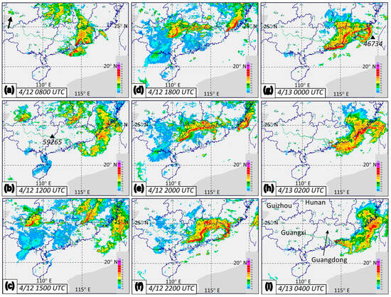
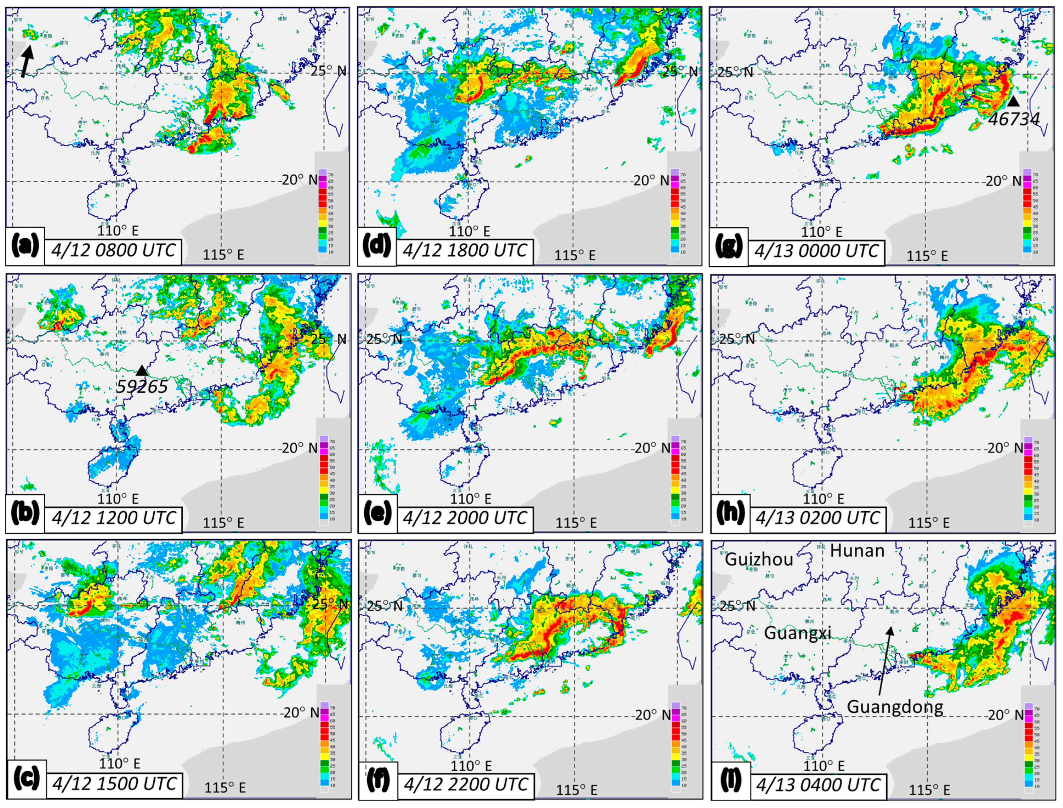
During 12–13 April 2016, another bow echo with a clear bulge developed and propagated across South China in a region of widespread convection (Figure 1). It produced surface wind gusts up to ~25 m s−1, with hail and heavy rainfall, as well as damage to many houses, buildings, infrastructures, and the power grid. While bad weather took place for over 24 h, the bow echo itself was intense and lasted for 15 h, with a relatively long lifespan in this region [28,29]. Therefore, it is a unique and interesting event that warrants detailed investigation. Due to its high intensity and long lifespan, we are particularly keen to understand the environmental conditions and favorable factors leading to its formation and development, as well as the reasons for why that part of the squall line formed the bow echo. To fulfill this goal, an ensemble of 20 high-resolution model simulations is performed, and, in terms of the reproduction of bow-echo features, the more successful members are compared and contrasted with the less successful ones. While the ensemble approach is still quite limited in the literature, e.g., [35,36], the important factors for the bow formation in the present event can be isolated in this way to augment our understanding on bow echoes in subtropical East Asia.
Figure 1.
Radar reflectivity composites (dBZ) over South China at selected times every 2, 3, or 4 h from (a) 0800 UTC 12 April to (i) 0400 UTC 13 April 2016, as labeled (0000 UTC = 0800 LST). The convection of interest is marked by the arrow in (a) at its initiation, and the two sounding sites used in Figure 6 are marked by the triangles in (b) for Wuzhou (59265) and (g) for Makung (46734). The names of provinces of China mentioned in text are also labeled in (i).
The remainder of this paper is arranged as follows. In Section 2, the data, case overview, synoptic conditions, numerical model, ensemble experiments, and methodology to analyze model results are described. The model results, including the control (CTRL) experiment and the other members, are described and discussed in Section 3. In Section 4, further discussion on the favorable environmental factors is provided. Finally, a summary and conclusions are offered in Section 5.
2. Data and Methodology
2.1. Data
The observational data used in this study include the following. To document the morphology and evolution of the bow echo during 12–13 April 2016, radar reflectivity mosaics from the China Meteorological Administration, as well as those from the Central Weather Administration (CWA) of Taiwan, were used. Surface and upper-level weather maps in East Asia from the CWA were employed for synoptic analysis, and soundings at selected sites were also used for thermodynamic conditions before the event.
For the ensemble model experiments, four widely used objective gridded analysis datasets by major centers during the case period were adopted as the initial/lateral boundary conditions (IC/LBCs): the National Centers of Environmental Prediction (NCEP) Global Forecast System (GFS) operational final (FNL) analysis [37,38]; the analysis of the NCEP Climate Forecast System version 2 (CFSv2) [39], both from the United States; the European Center for Medium-Range Weather Forecast (ECMWF) Reanalysis (ERA)-Interim [40,41]; and the Japan Meteorological Agency (JMA) Global Spectral Model Analysis (GANAL) [42,43,44]. With different horizontal resolutions but all at 6 h intervals, these four datasets will be further described later in Section 2.5. Among them, the NCEP FNL will also be used to compare and validate the CTRL experiment in Section 3.1. Based on model results, the circulation patterns and environmental conditions among these datasets will also be compared to identify the factors favorable for the bow echo case.
2.2. Case Overview
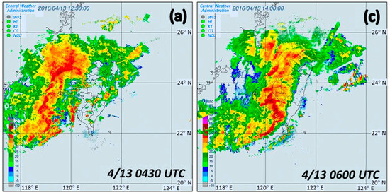
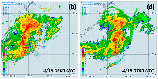
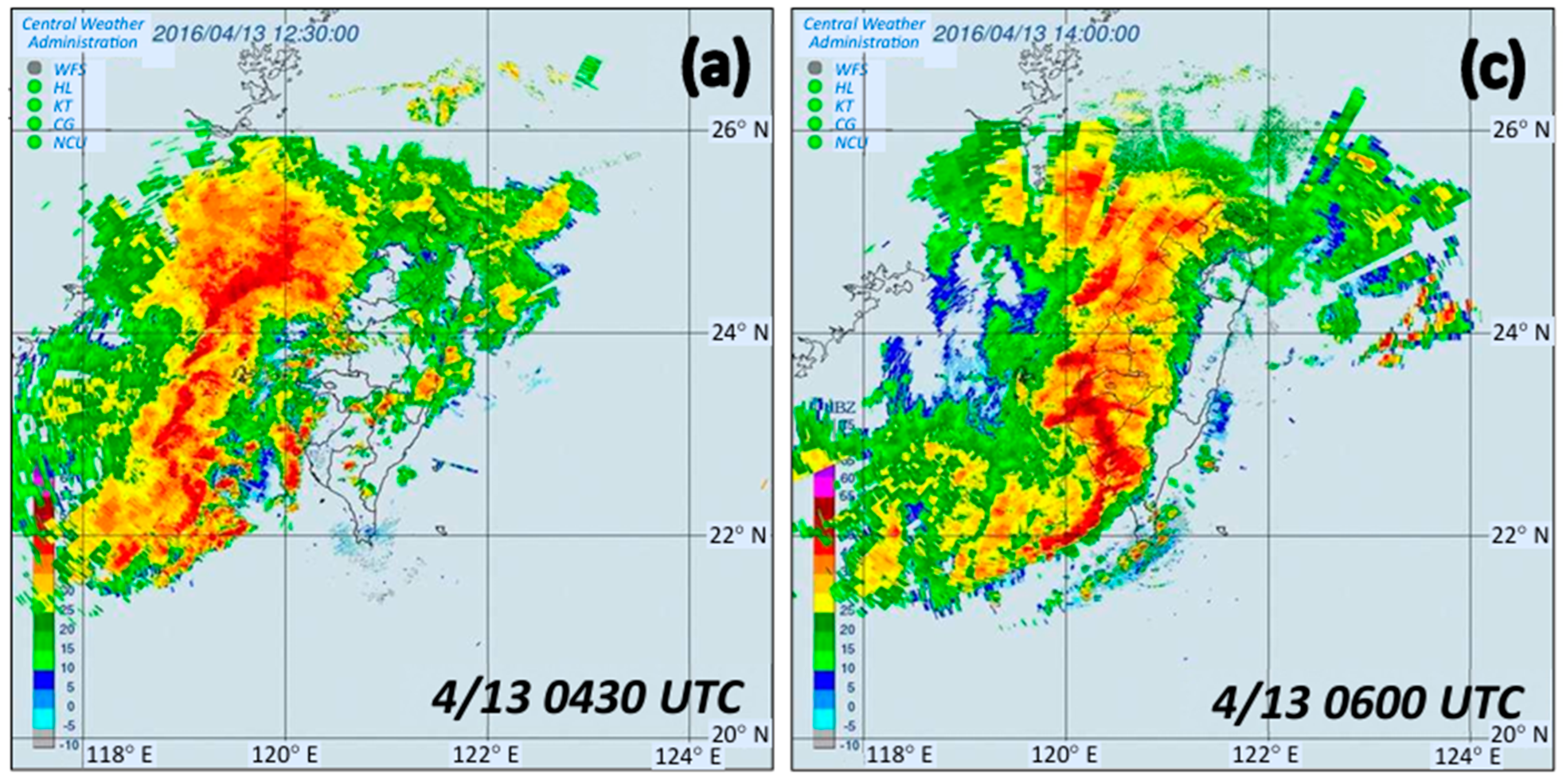
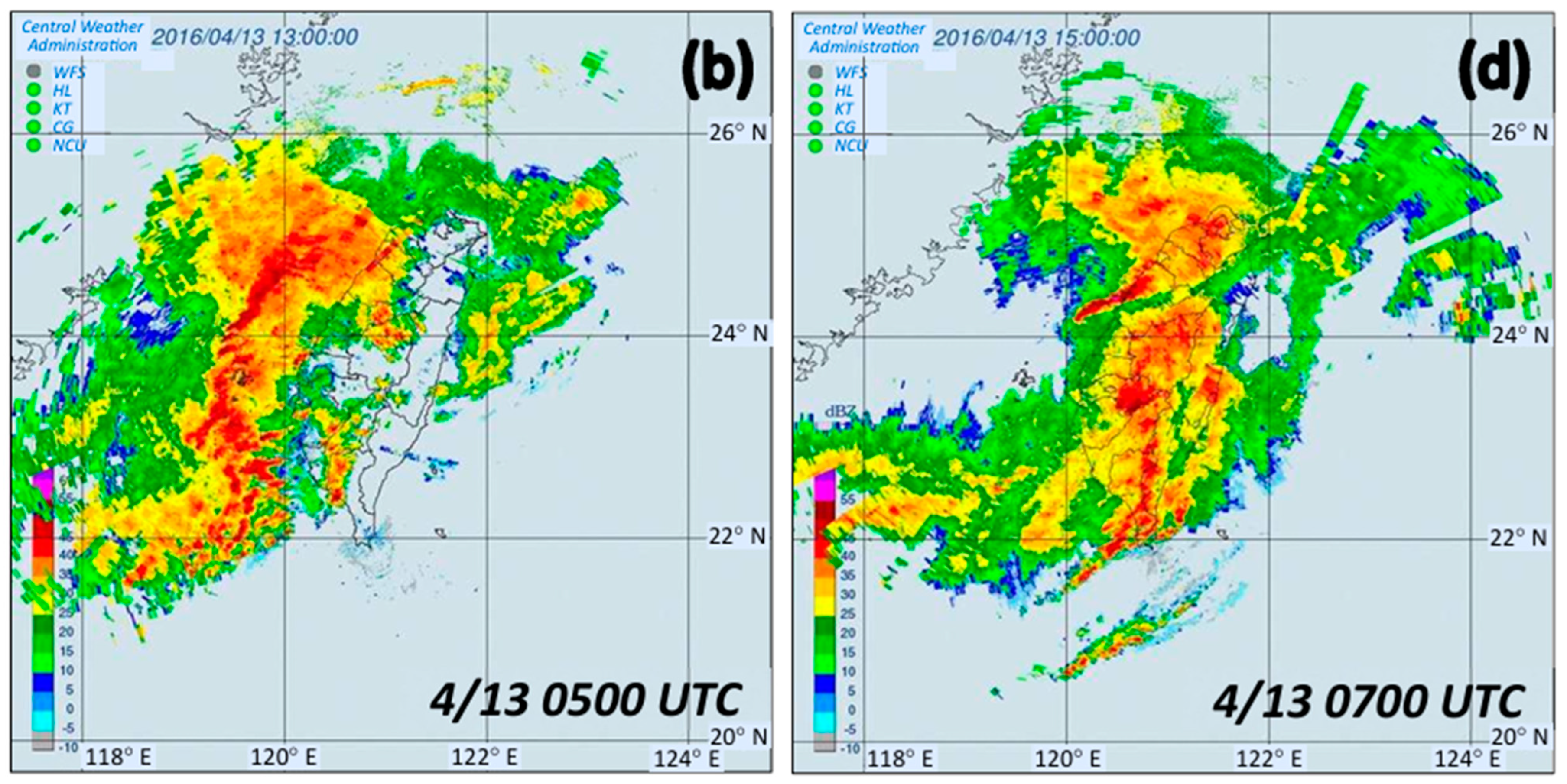
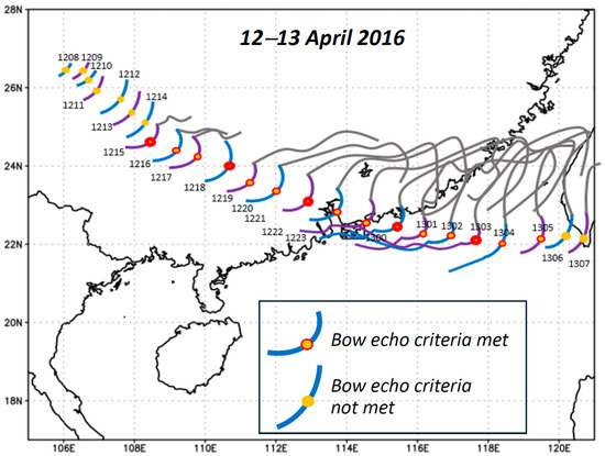
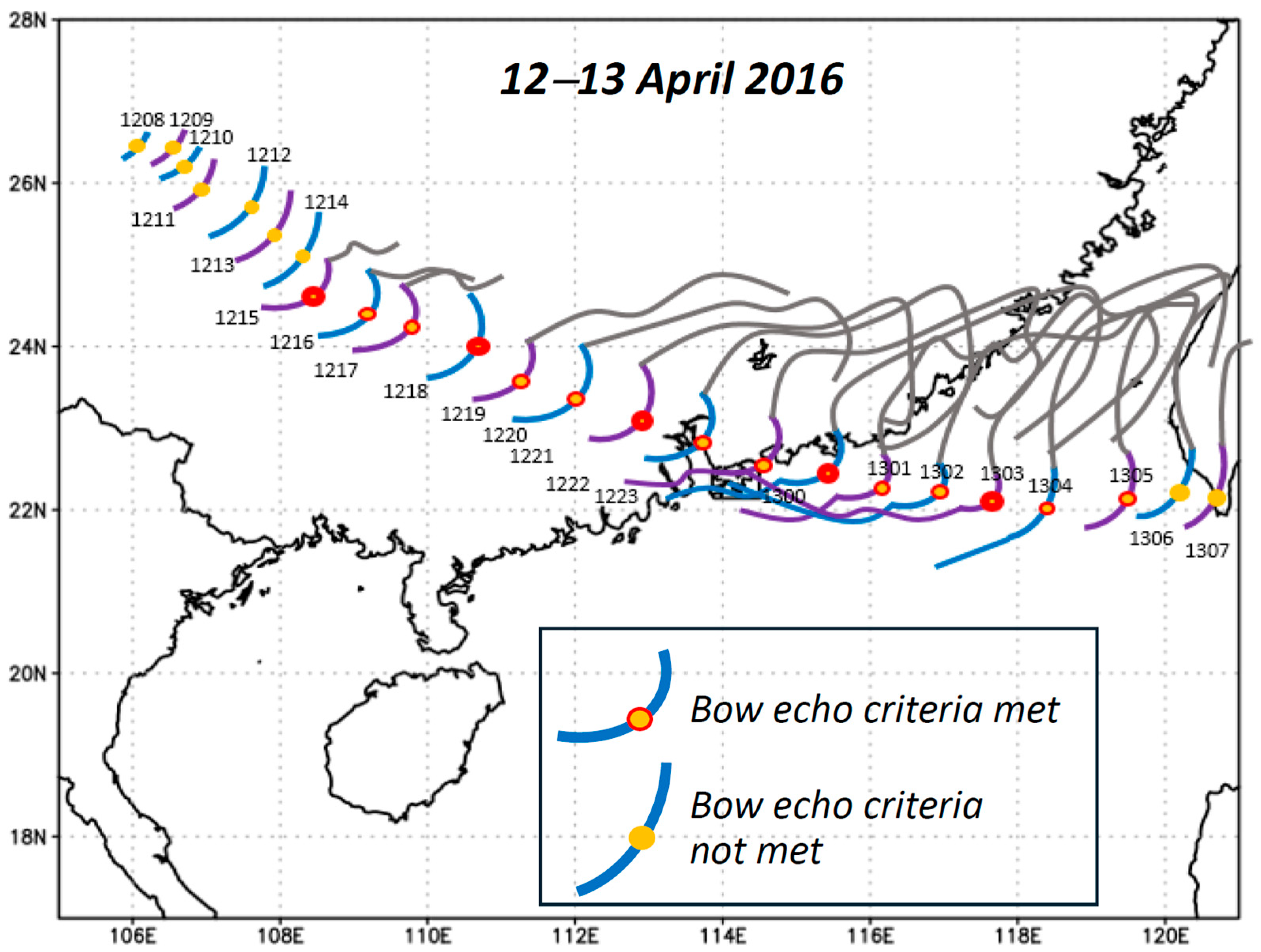
The bow echo in this study occurred during 12–13 April 2016 (Figure 1). The convective system initiated over Guizhou Province in Southwestern China in the afternoon of 12 April (Figure 1a, 0800 UTC = 1600 LST) near a frontal zone (to be shown shortly) and subsequently propagated southeastward while intensifying (Figure 1a–c). By the early hours of 13 April, the system had evolved into a well-defined bow echo (Figure 1c,d), affecting Guangxi and Guangdong Provinces and producing severe weather, including strong winds, heavy rainfall, and hail (Figure 1d–i). When the bow echo moved into the Taiwan Strait, it was also captured by the radar network in Taiwan (Figure 2). It made landfall in Southern Taiwan and lasted through 0700 UTC 13 April. Here, using the criteria of [45] for convective lines near Taiwan (i.e., maximum radar reflectivity ≥ 20 dBZ, length ≥ 150 km, and duration ≥ 3 h), plus a clear bulge in reflectivity, the lifecycle and propagation of this bow echo observed by radars have been mapped and shown in Figure 3. Thus, since the system reached the criteria at 1500 UTC 12 April, it persisted as a bow echo for approximately 15 h, representing a relatively long-lived event in South China and Taiwan, as mentioned [28,29]. In Figure 3, one can see that the convective line moved relatively slowly at the beginning after formation but started to propagate rapidly once it evolved into a bow echo. Its mean propagation speed was 22.1 m s−1 during the bow-echo stage compared to 19.2 m s−1 over its entire lifespan. In fact, in Figure 1, a second bow echo appeared around 1800–2000 UTC 12 April as it moved across the Northern Taiwan Strait, but its lifespan was much shorter and lasted only a few hours (Figure 1d,e). Therefore, certain favorable factors must have been there to enhance the bow echo studied herein.
Figure 2.
Radar reflectivity composites (dBZ) from the CWA radars in Taiwan at (a) 0430, (b) 0500, (c) 0600, and (d) 0700 UTC on 13 April 2016 (0000 UTC = 0800 LST).
Figure 3.
Hourly position and movement of the convective system/bow echo from 0800 UTC 12 to 0700 UTC 13 April 2016, as determined from the radar observation (0000 UTC = 0800 LST). The apex of the bow echo or middle point of the convective line are marked by the circle (thickened every 3 h during bow-echo stage), and the legend illustrates the meaning of different symbols.
2.3. Synoptic Environment and Instability
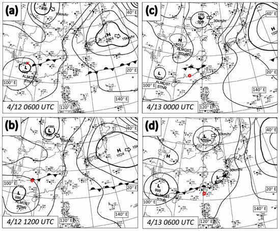
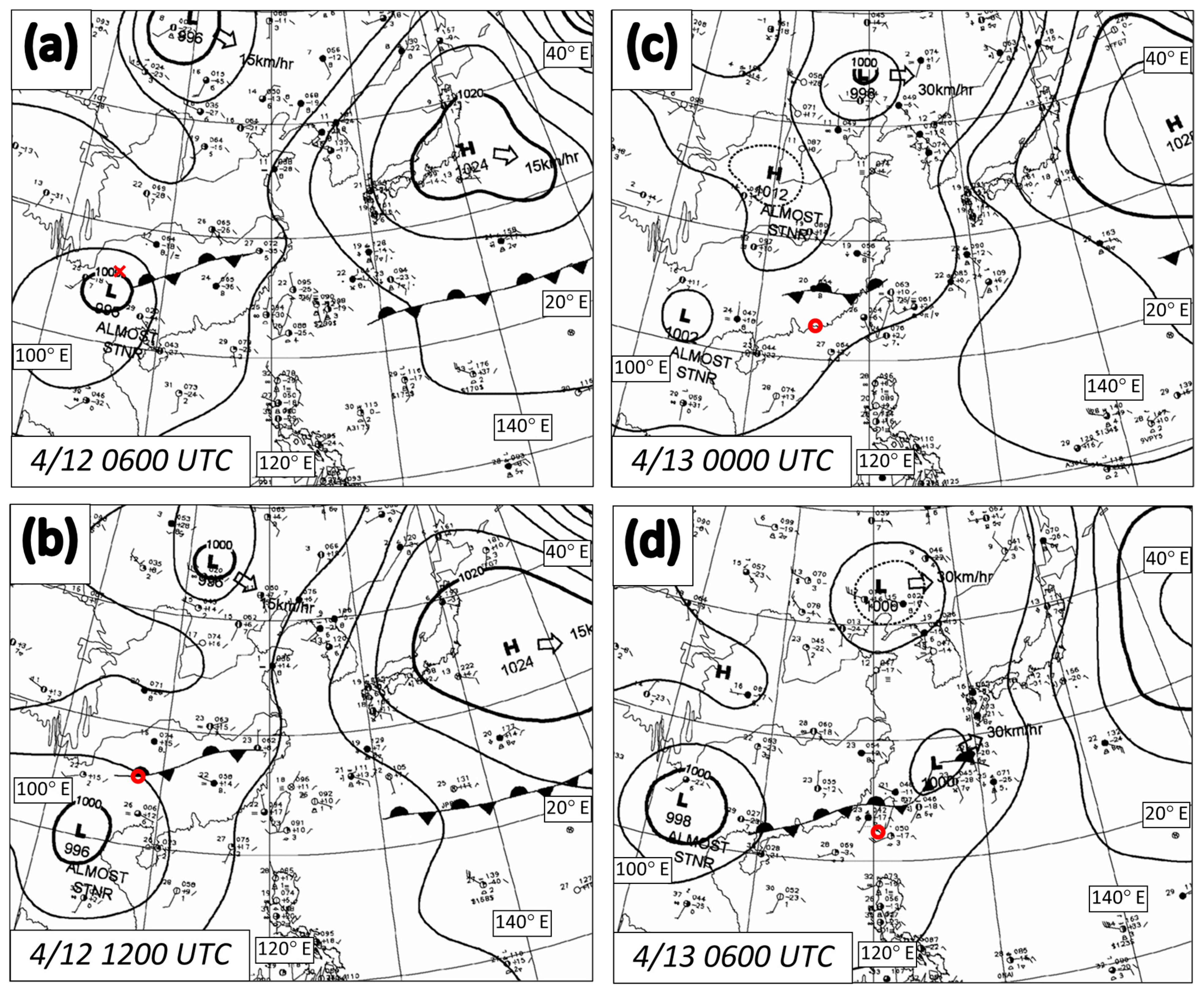
From the CWA surface weather maps, a stationary front is seen to exist over South China, to the south of the Yangtze River, at 0600 and 1200 UTC 12 April 2016, separating relatively warm air to the south from cooler air to the north (Figure 4a,b). While the front provided some lifting, a low-pressure appeared at its western end, transporting warm air toward the front. Near the front and low center, the convection that would evolve into the bow echo was triggered by 0800 UTC (red “x” in Figure 4a). Since the bow echo was moving at a high speed, it gradually propagated farther south, away from the frontal zone, and well into the warm side. By 0000 UTC 13 April, its apex had already moved offshore (red open circle), and the front had also started to move south to affect Guangxi and Guangdong Provinces (Figure 3 and Figure 4c). Six hours later, the front almost reached the coastline of China, though the bow echo had already hit Southern Taiwan (Figure 2c, Figure 3, and Figure 4d).
Figure 4.
The CWA surface weather maps for (a) 0600 and (b) 1200 UTC 12 April and (c) 0000 and (d) 0600 UTC 13 April 2016. Black solid lines are isobars of sea-level pressure (hPa) analyzed every 4 hPa (thickened every 20 hPa). The apex of the bow echo is marked by the open red circle in (b–d), and its initiation location at 0800 UTC (see Figure 1 and Figure 3) is marked by the red “x” in (a).
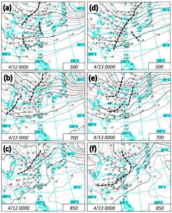
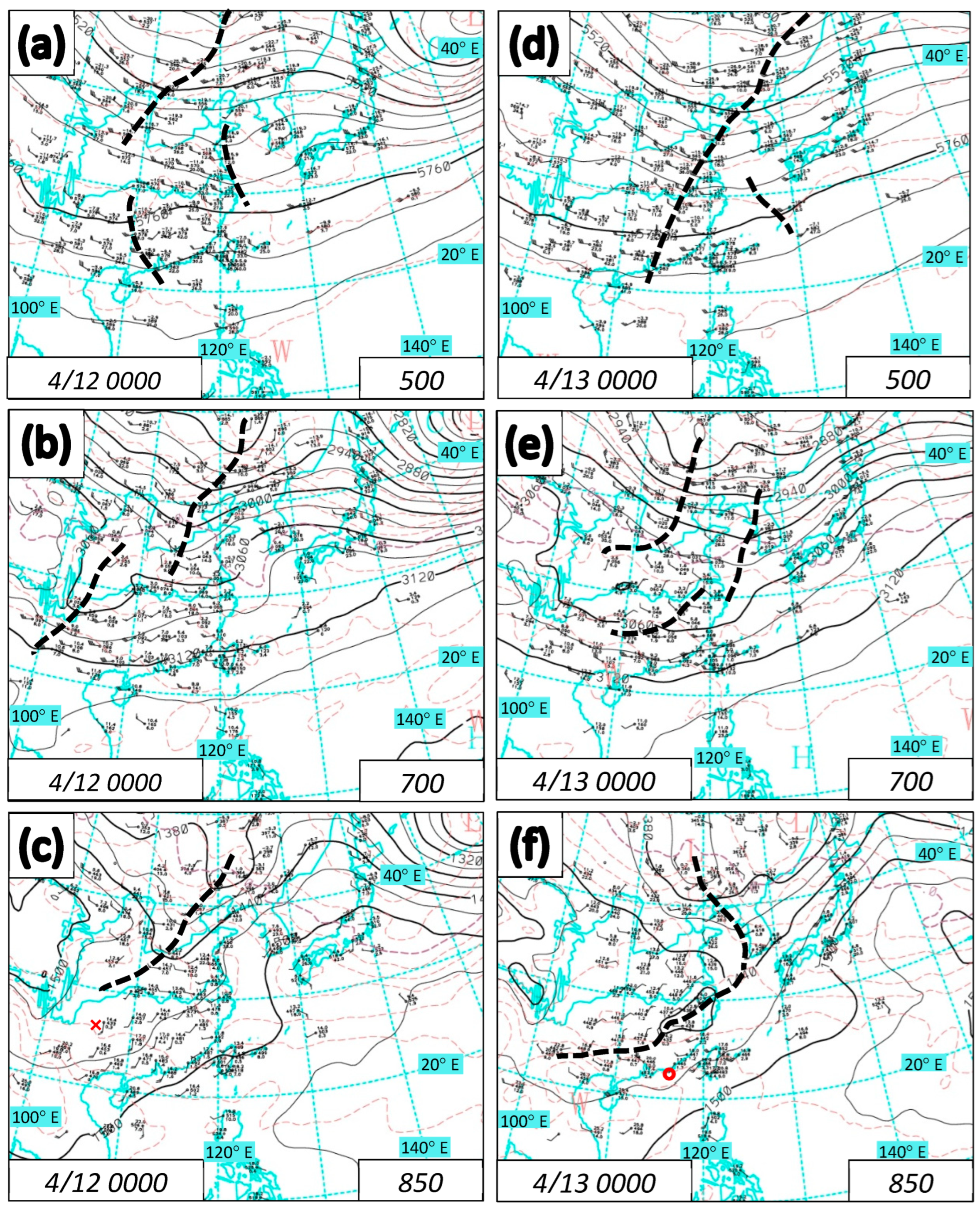
The upper-air weather maps show that at 0000 UTC 12 April, the trough at 850 hPa was located north of the Yangtze River and a southwesterly flow of 10–15 kts prevailed over the entire South China (Figure 5c). In other words, the stationary front at the surface was shallow at this time. The flow over South China turned into west–southwesterly to westerly, strengthening to 20–30 kts at 700 and 500 hPa, with an approaching short-wave trough from the west at both levels (Figure 5a,b). The advancing troughs provided rising motion ahead and the veering of winds with height indicated warm air advection, both favoring convective initiation (CI). In addition, the strong vertical wind shear was a vital ingredient for the deep convection to organize into squall lines and bow echoes, as mentioned. One day later at 0000 UTC 13 April, as the 500 hPa trough moved through the area (Figure 5d), the front at 850 hPa deepened significantly over South China, with a clear cyclonic circulation and a low-pressure center north to northeast of the bow echo, and became vertically coupled with the surface front (Figure 5e). At 700 hPa, a corresponding wind-shift line also appeared (Figure 5f), so the frontal system became much deeper. Note that around this time, this developing front-trough system provided northwesterly flow throughout low levels at the backside of the bow echo, which was propagating toward the coast of South China. In other words, the circulation of this deepening front-trough system was feeding northwesterly flow into the backside of the bow echo, a point that will be further discussed later. Apparently, the northwesterly flow and the northerly winds behind the 850 hPa front also pushed the front-trough system southward.
Figure 5.
The CWA weather maps at (a) 500 hPa, with wind barbs (knots), geopotential height contours (gpm, black) every 60 gpm, and isotherms (°C, red dash) every 5 °C; (b) 700 hPa, with wind barbs (knots), geopotential height contours every 30 gpm, and isotherms every 3 °C; and (c) 850 hPa, with variables and plotting method as in 700 hPa, at 0000 UTC 12 April 2016. The troughs are marked by thick dashed lines. (d–f) are the same as in (a–c), except at 0000 UTC 13 April 2016. Locations of the convective system are also marked in (c,f) as in Figure 4.
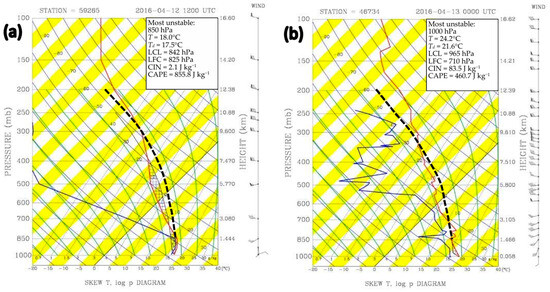
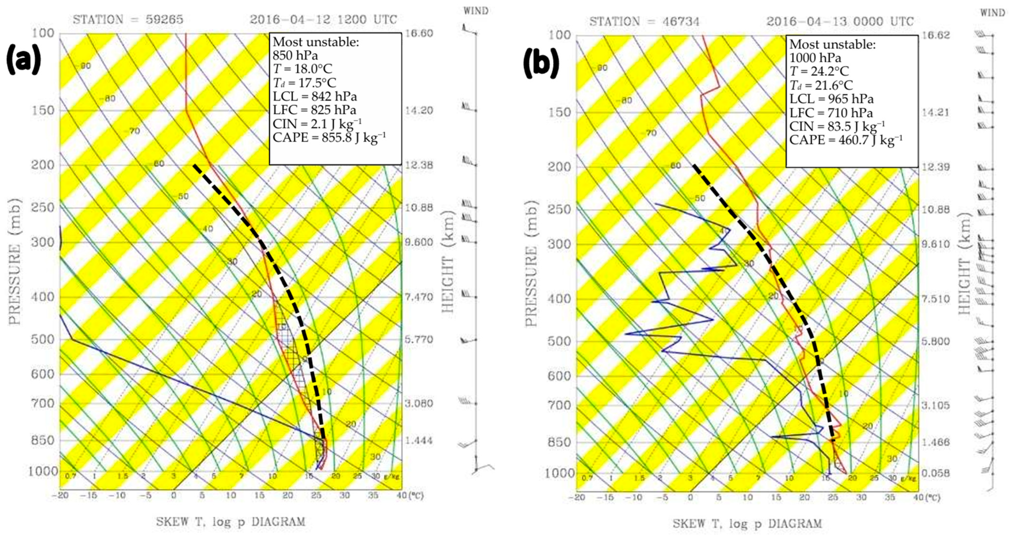
For thermodynamic conditions prior to the convection, two soundings were selected and are shown in Figure 6. The sounding at Wuzhou (59,265) at 1200 UTC 12 April (Figure 6a), about 8 h before the passage of the bow echo (see Figure 1b,e), indicates that the parcel from the most unstable level, located at 850 hPa, possessed a respectable amount of CAPE—about 856 J kg−1—with nearly no convective inhibition (CIN). In fact, if uplifted from roughly 950 hPa and closer to the surface, a parcel there would have nearly the same CAPE. The sounding at Makung (467,34) on the island of Penghu over the Taiwan Strait at 0000 UTC 13 April was launched about 4 h before the convective line passed through. A surface parcel would possess about 461 J kg−1 of CAPE with some CIN of 84 J kg−1 to overcome and reach free ascent. Thus, the thermodynamic conditions in the region were also supportive to convection. Overall, as shown in Figure 4, Figure 5 and Figure 6, the synoptic environment of the bow echo was quite favorable for the initiation and maintenance of deep convection, and for the development of the linear convection and bow echo as well.
Figure 6.
The soundings with vertical wind profile (knots) at (a) Wuzhou (59265) at 1200 UTC 12 April and (b) Makung (46734) at 0000 UTC 13 April 2016. Selected relevant parameters for the most unstable level are given inside the box at the top-right corner, and the process curve is depicted by the thick dashed line. Locations of the two sites are marked in Figure 1b,g.
2.4. Numerical Model
In this study, all numerical experiments were conducted using the Cloud-Resolving Storm Simulator (CReSS, version 3.4.2), developed by Nagoya University of Japan [46,47]. The CReSS model is a nonhydrostatic model equipped with comprehensive cloud microphysics schemes, allowing for detailed representation of convective clouds and MCSs alike. In this study, the single-moment cold-rain cloud microphysics scheme based on [48,49,50,51,52] is adopted. The model has been widely applied to study convective storms, tropical cyclones, heavy rainfall events, and other types of severe weather, e.g., [53,54,55,56,57,58]. A detailed description of the model can be found in [47] and some studies referenced above.
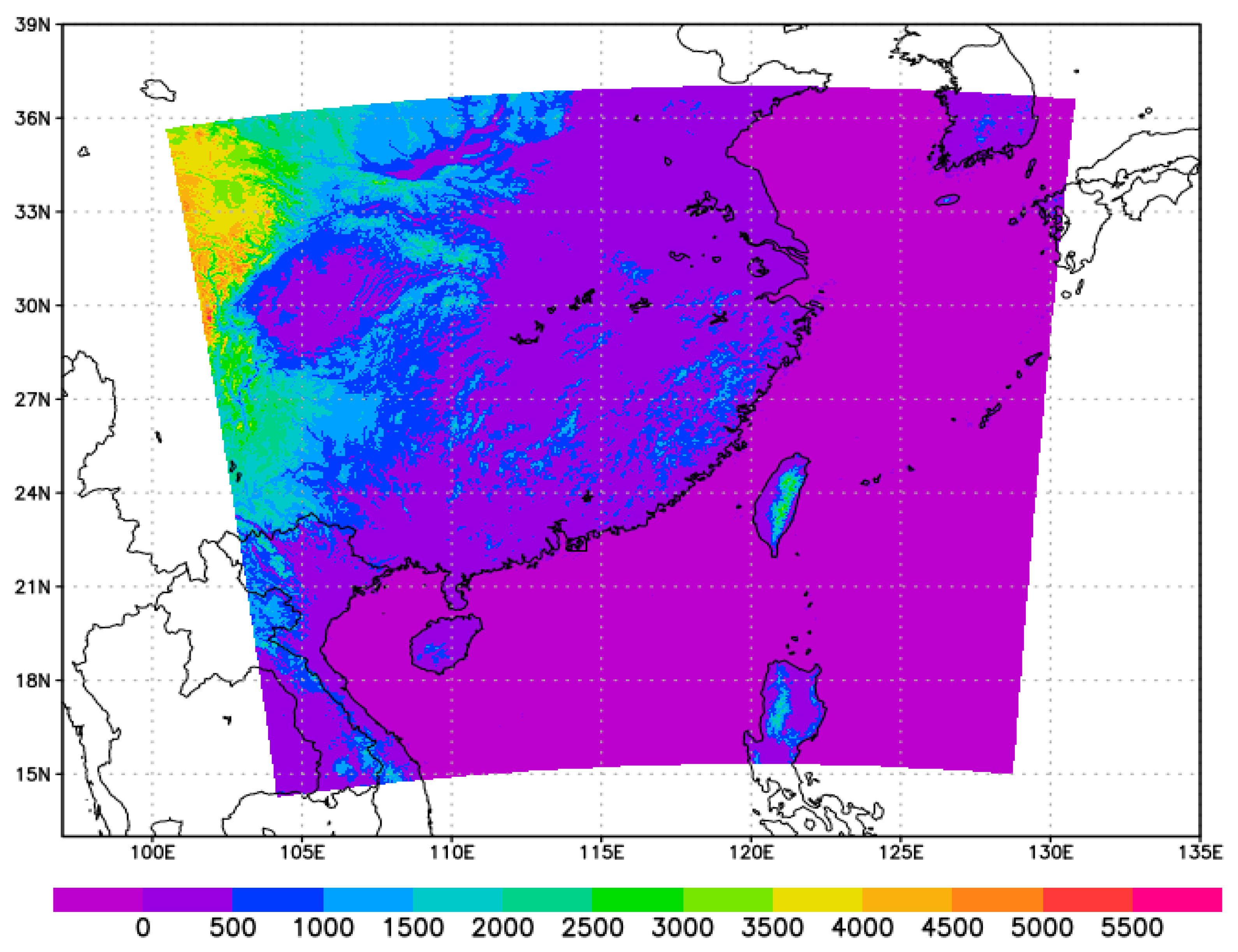
The CReSS model utilizes a single high-resolution domain (no nesting), with a horizontal grid spacing of 2 km here. The model domain consists of 1350 × 1200 grid points in the horizontal (Figure 7) and 40 vertical levels with a model top at 20 km (averaging 500 m apart, Table 1). The vertical coordinate is, in fact, a hybrid based on height with terrain-following coordinates below the lowest constant-height level, which is set to 12 km. For time integration, CReSS uses a split time-step scheme [59,60], with a large time-step of 4 s for low-speed modes and a small time-step of 2 s for acoustic and gravity waves. At the bottom of the model, topographic data and sea surface temperature (SST) analyses from the National Oceanic and Atmospheric Administration (NOAA) were also provided [61]. Model outputs were saved at hourly intervals for subsequent analysis. Table 1 provides a list for the major specifications of the model common to all experiments.
Figure 7.
Model domain (color area) and topography (m, scale at bottom).
Table 1.
Configurations and physical options of CReSS that were common to all experiments in this study.
2.5. Design of Ensemble Experiment
To examine the sensitivity of the bow echo in the CReSS simulation and to identify the important factors affecting the results, an ensemble approach is adopted in this study. For this purpose, an ensemble is produced using four different analysis datasets by major centers with five different initial times as IC/LBCs, resulting in a total of 20 ensemble simulations. As mentioned, the four datasets include the NCEP GFS FNL, the NCEP CFSv2, the ERA-Interim by the ECMWF, and the JMA GANAL, all at 6 h intervals [37,38,39,40,41,42,43,44]. In Table 2, these datasets and the five initial times are listed. Since ECMWF and JMA provide only one dataset each, it may be denoted simply by the agency name later. All ensemble simulations employed identical model configurations and physical parameterizations, differing only in their IC/LBCs (and simulation length). This strategy allows for an intercomparison among simulation results of the bow echo using somewhat different but widely used IC/LBC products from different meteorological centers.
Table 2.
The four datasets for IC/LBC and five initial times used to produce the CReSS ensemble experiments in this study.
2.6. Analysis of Model Results
As the last initial time is 0600 UTC 12 April and all runs end at 1800 UTC 13 April 2016, they can cover the entire lifespan of the bow echo (Table 2). In all 20 experiments, organized convection was produced in South China during 12–13 April. These results were evaluated against the observation for morphology, duration, propagation speed, and structural characteristics of the bow echo—mainly subjectively—for an overall assessment. The experiment that best reproduced the bow echo is identified as the CTRL (the one initialized at 0000 UTC 12 April using NCEP FNL as IC/LBCs), which is to be validated in Section 3.1. Among all 20 runs, certain members simulated the bow echo more successfully, with a more distinct bulge, more accurate track, and longer duration. Others, on the other hand, failed to maintain an organized convective line long enough, thus with a shorter lifetime, and were less successful. Subsequently, the best six of these were selected as the “good member” (GM), as they produced a clearer bow shape with a longer duration. Conversely, the worst six members were also chosen as the “bad member” (BM). By comparing the composite results of GMs and BMs using the apex as the common point of reference, further investigation of key differences in the structure and intensity of the bow echo, including those of the RIJ, can be identified. Similarly, differences in the environment that could contribute to the differences in the bow echo and its longevity, such as moisture supply and circulation patterns, are also examined and discussed.
3. Model Results
3.1. Control Experiment and Validation
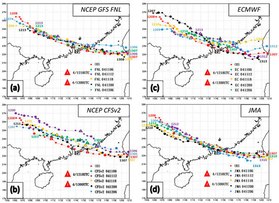
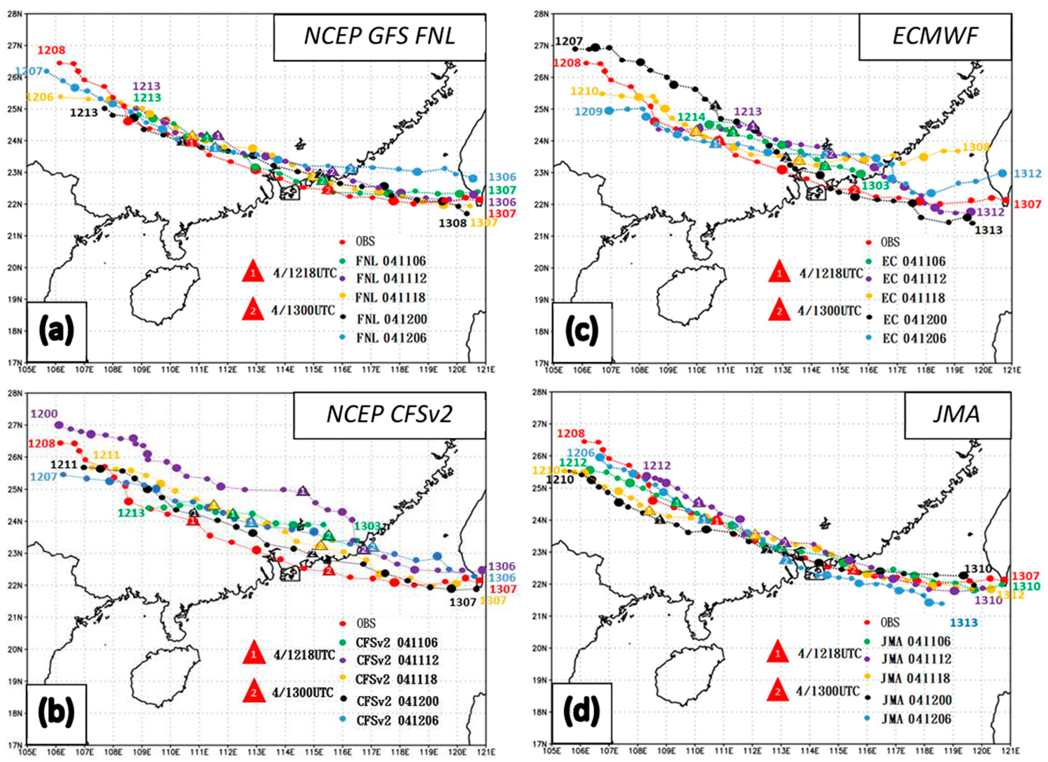
As mentioned, widespread and organized convection over South China during 12–13 April 2016 was captured in all 20 ensemble experiments. While the bow echo was reproduced more faithfully in many of them, the bow-shaped feature was not as distinct nor even barely discernible in some other runs. Nevertheless, even in the latter cases, a convective line could still be identified. Thus, using the method as for Figure 3, the apex of the bow echo, or the center of the corresponding convective line, during its lifespan in each of all 20 runs was identified, as shown in Figure 8. Here, the column-maximum mixing ratio of precipitation (rain + snow + graupel) was used for identification, as radar reflectivity is mainly caused by such larger, falling particles. As seen, while runs using some datasets produced fairly concentrated tracks for the bow echo/line convection (e.g., NCEP FNL and JMA) and others less so (e.g., NCEP CFSv2), all systems have a long lifespan and propagation direction comparable to the observed bow echo. Notably, these lifespans and the propagation speeds during the bow-echo phase (around 20 m s−1) are significantly longer and faster than averaged squall lines and MCSs in South China [27,28,29,62]. In Figure 8, in earlier runs (green and purple), the convection also tends to initiate at a later time, e.g., during 1200–1400 UTC 11 April.
Figure 8.
Hourly position (dots) and movement of the bow echo/convective system in the 20 ensemble experiments using (a) NCEP FNL, (b) NCEP CFSv2, (c) ECMWF ERA, and (d) JMA GANAL as IC/LBCs, as determined from the distribution of column-maximum mixing ratio of precipitation (g kg−1, rain + snow + graupel). Experiments with different initial times are differentiated by color (see legend) with starting/ending times labeled (in format of “ddtt” for date/time in UTC), and the observed track (red) is also plotted (same as in Figure 3). During bow-echo stages, the apex positions are enlarged every 3 h, and the two triangles (with numbers) mark the positions at 1800 UTC 12 (first) and 0000 UTC 13 (second) April 2016.
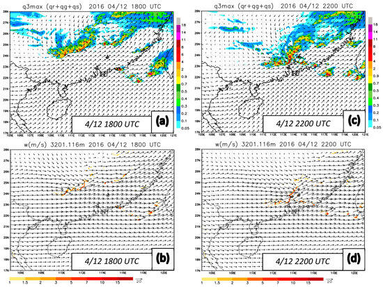
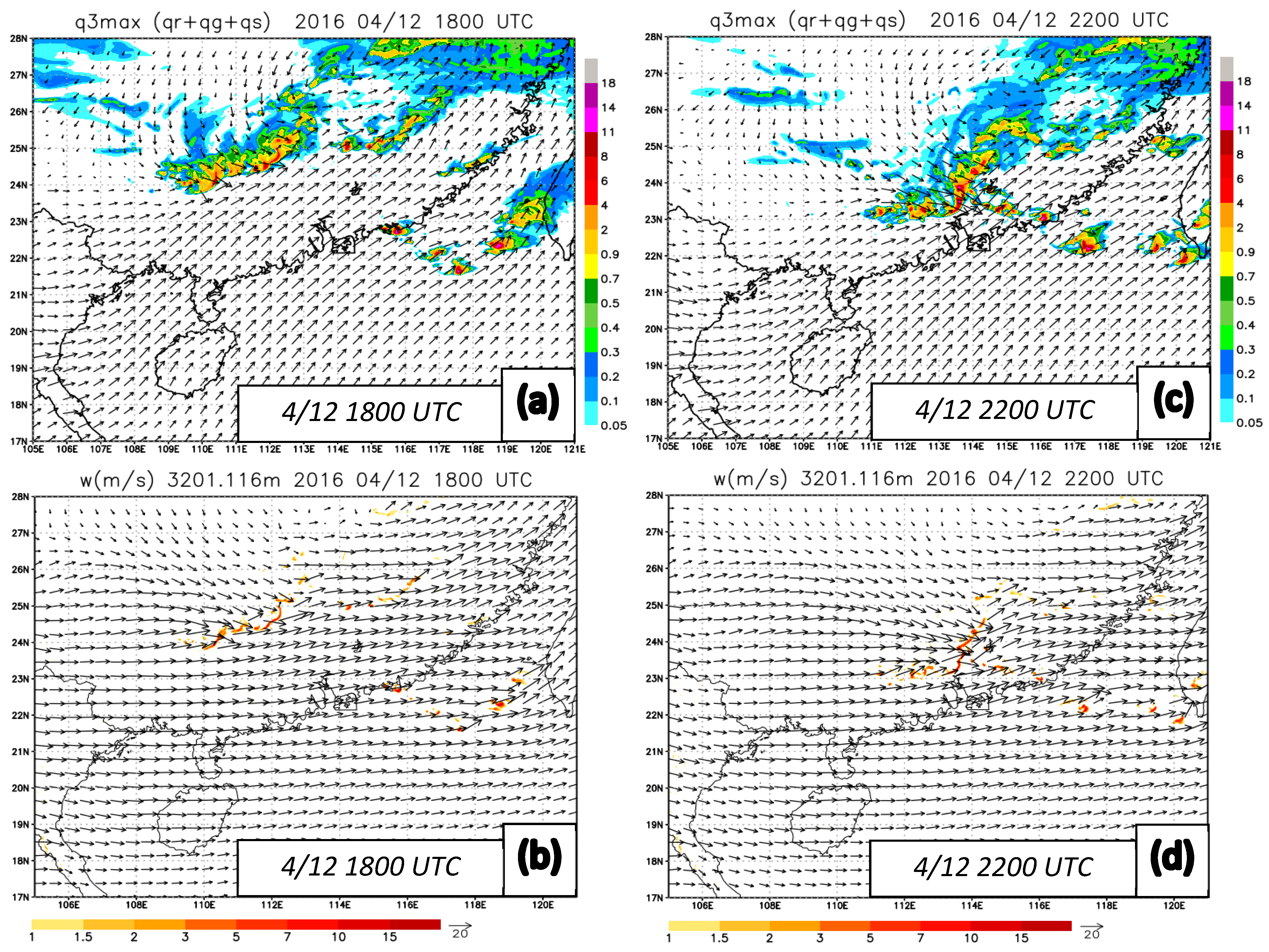
From Figure 8 and the loops of other relevant plots (e.g., kinematic structure and rainfall pattern), the experiment initialized at 0000 UTC 12 April using NCEP FNL analysis was determined to best reproduce the bow echo and was thus designated as the CTRL (track in black in Figure 8a). The characteristics of this system in the column-maximum mixing ratio of precipitation and vertical motion are shown in Figure 9 at two instances: 1800 and 2200 UTC 12 April 2016. At 1800 UTC (Figure 9a), the system in the CTRL has already evolved into a bow echo, with its apex near 24.0° N, 110.4° E and a clear rear inflow at the level of z = 1594 m (near 850 hPa). To the south of the system, the low-level flow is coming from the southwest at about 16 m s−1 and is quite uniform. Farther up at 3201 m, the strong westerly to west–northwesterly flow, over 20 m s−1 at some places at the backside and feeding into the bow echo, is also visible (Figure 9b). At this time, the location of the bow echo is very close to the observation (also Figure 1d and Figure 8a), although the system in CTRL is perhaps somewhat less pronounced in its bow shape. As noted, the low-level trough extended from the bow echo toward the northeast, with a low-pressure center near 28° N, 115° E. Four hours later at 2200 UTC, the bow echo in CTRL evidently has further intensified along with its RIJ at both 1594 and 3201 m (Figure 9c,d), which is also consistent with the observation (see Figure 1f).
Figure 9.
(a) Maximum total mixing ratio of precipitating particles (g kg−1, rain + snow + graupel, color) and horizontal wind vectors (m s−1, reference length at bottom) at z = 1594 m; (b) upward motion (m s−1, color, scale at bottom) and horizontal wind vectors (m s−1) at z = 3201 m at 1800 UTC 12 April 2016 in CTRL. (c,d) are the same as in (a,b), except at 2200 UTC.
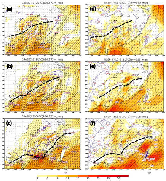
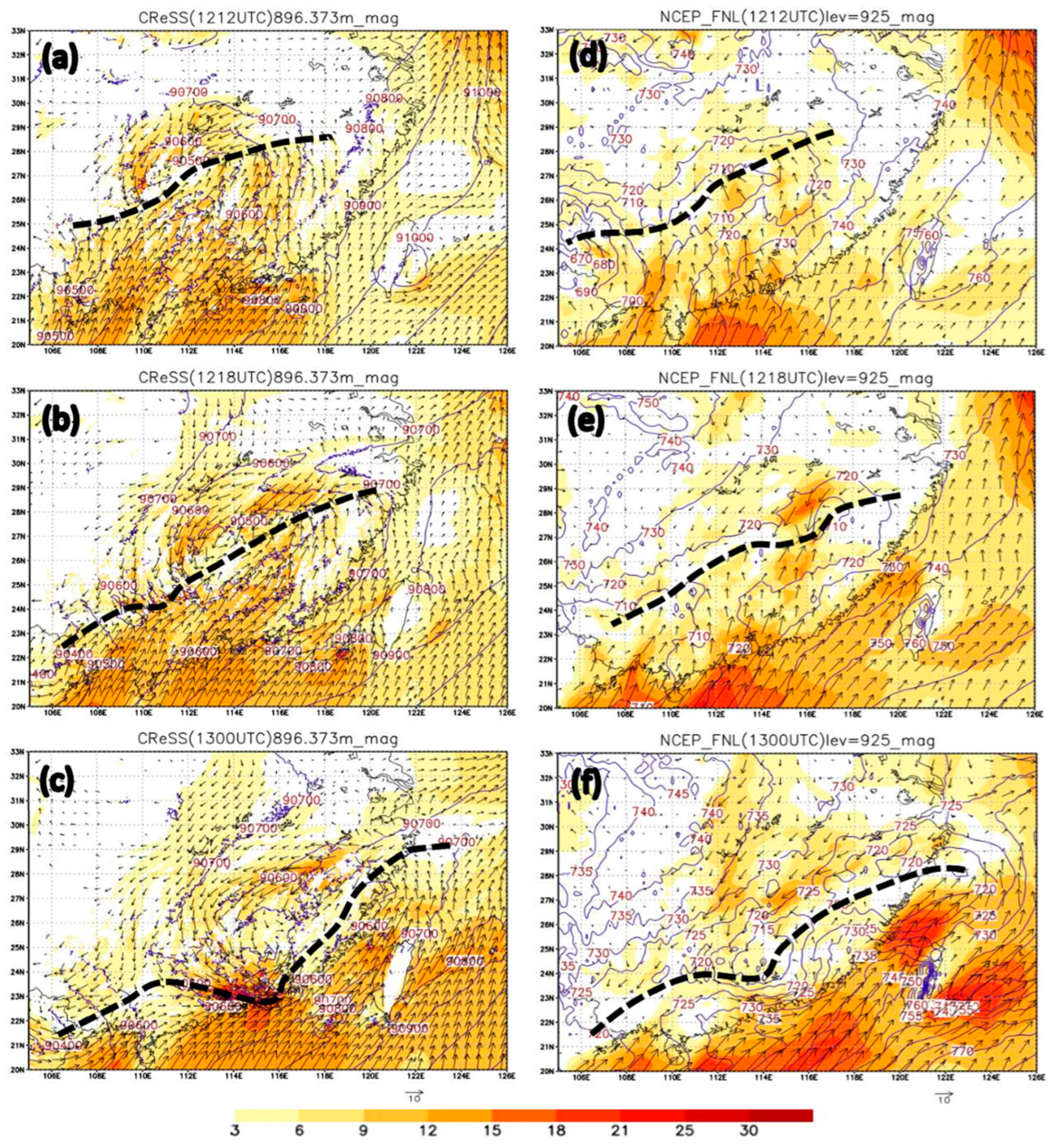
As an additional verification, Figure 10 shows a comparison of NCEP FNL analysis at 925 hPa with the CTRL at the output level of z = 896.4 m (closest to 925 hPa) at three different times of 1200 and 1800 UTC 12 April and 0000 UTC 13 April 2016. The CTRL is seen to reproduce the low-level trough at roughly the correct location with clear cyclonic circulation, but the southwesterly flow on the warm side of the trough tends to be slightly weaker in the model, presumably linked to its more rugged terrain (Figure 10). With the development of the bow echo, the distortion of the trough in the CTRL toward the later stage at 0000 UTC 13 April is also more evident—somewhat expected in such high-resolution experiments. Thus, the orientation and movement of the bow echo, as well as the main precipitation region, are reproduced quite well in the CTRL. However, certain deficiencies can be noted, as the convection with a circular shape to the north and east of the bow echo around 2200 UTC 12 April is not fully captured (see Figure 1f and Figure 9c), and some peripheral convective cells are also weaker than observed. Despite these limitations, the CTRL provides a good and realistic simulation, as well as a reasonable baseline for further comparison and evaluation on the performance of other ensemble members.
Figure 10.
Pressure field (Pa, isobars every 1 hPa) and horizontal wind vectors (m s−1, reference length at bottom) at z = 896.4 m in CTRL at (a) 1200 and (b) 1800 UTC 12, and (c) 0000 UTC 13 April 2016. (d–f) are the same as in (a–c), except for geopotential height (gpm, contours every 10 gpm) and horizontal wind vectors (m s−1) at 925 hPa in NCEP FNL analysis at the three times. Thick dashed lines indicate trough/wind-shift line.
3.2. Important Factors from Ensemble Experiment
Based on how well the bow echo was reproduced in the experiments, all 20 ensemble members were classified into three groups as mentioned: six GMs, six BMs, and eight others in between (Table 3). Using the apex during the bow-echo stage (or the center of line convection otherwise) as the common reference point, i.e., the origin (see Figure 8), the CReSS model outputs in the GM and BM groups are extracted to produce composites using arithmetic mean for comparison. Also, in each run, the time with the most pronounced bow shape is identified as t = 0 h, as shown in Table 4, and the following five phases are used for composites: P1 (t = −6 to −4 h), P2 (t = −3 to −1 h), P3 (t = −1 to +1 h), P4 (t = +1 to +3 h), and P5 (t = +4 to +6 h). These phases roughly correspond to the formation, development, maturation, weakening, and dissipation stages in the lifecycle of the bow echo (or line convection), and each composite is made from 18 fields (6 members × 3 output times). By comparing the composites of GMs and BMs from P1 to P5, we can identify differences in structure and intensity of the bow echo between GMs and BMs, and subsequently, the key differences in their environment that contributed to their eventual differences in the CReSS simulations.
Table 3.
The classification results of the 20 ensemble members in this study, including the six GMs (GM-1 to GM-6, while CM-1 is CTRL) and six BMs (BM-1 to BM-6).
Table 4.
The time identified as having the most pronounced bow shape (i.e., t = 0 h and mid-point of P3, all in UTC) in each of the members in the GM and BM groups.
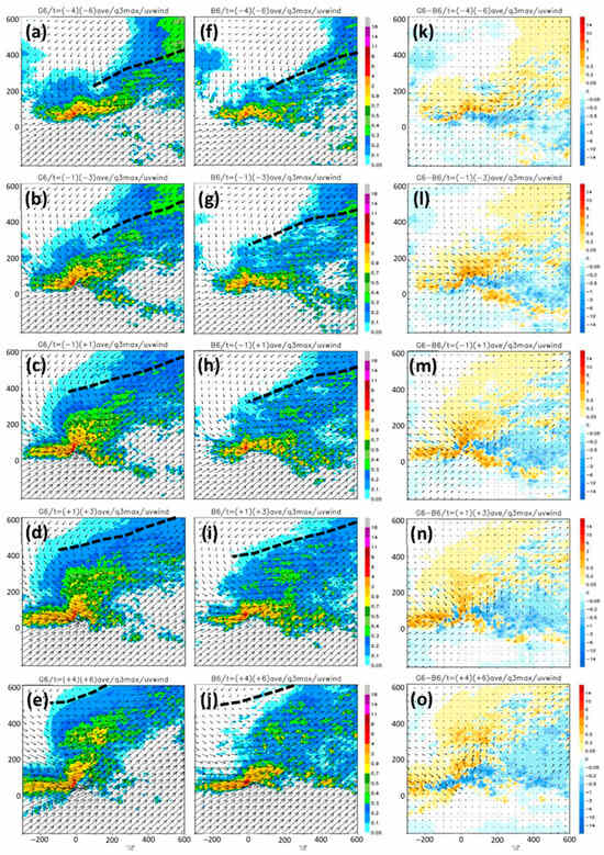
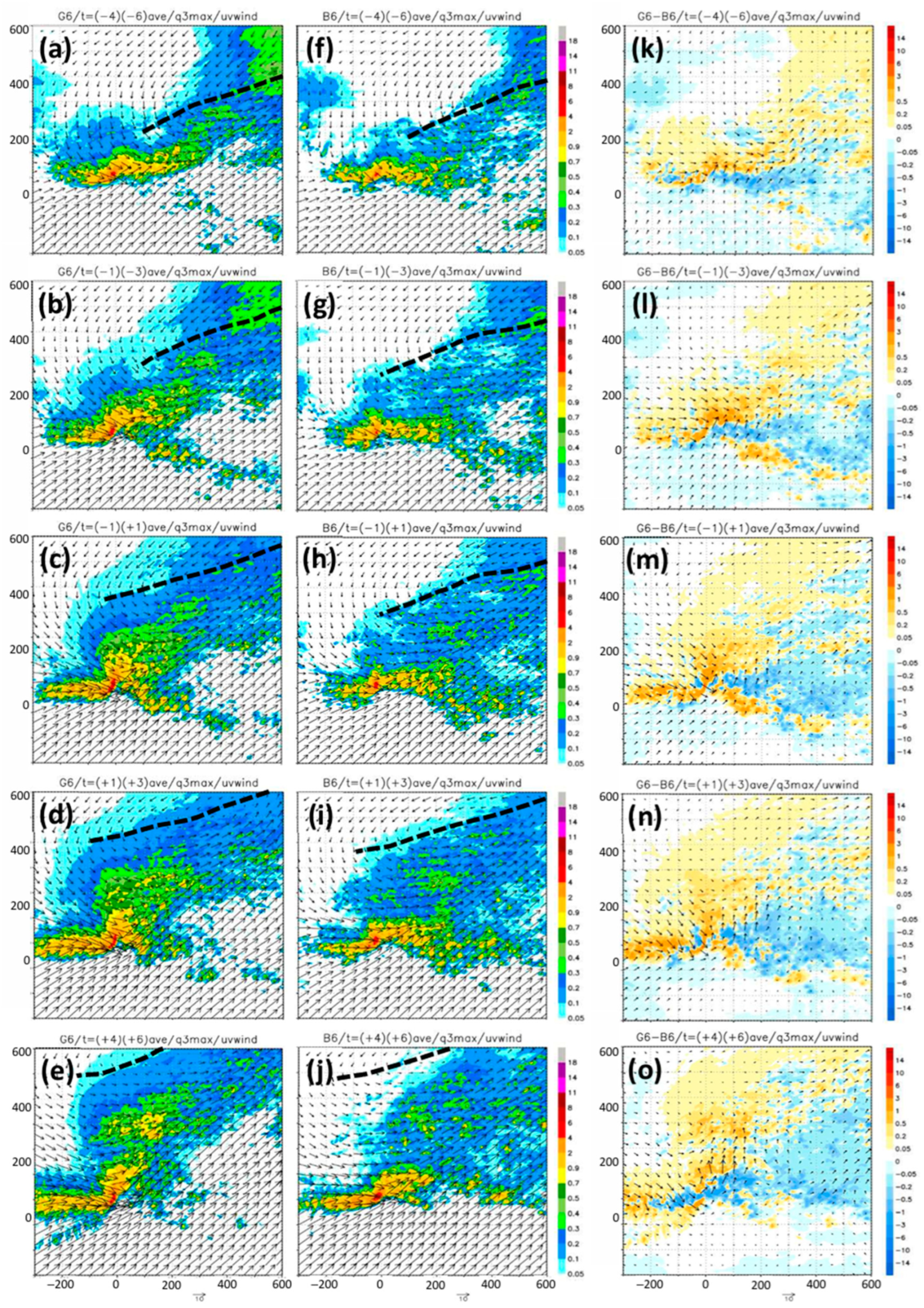
In Figure 11, the composites of the precipitation mixing ratio and low-level wind field at z = 1594 m (as in Figure 9a,c) from P1 to P5 for the GM (left column) and BM groups (middle column) are shown for a square region from −300 to +600 km in both x and y directions (i.e., 900 km × 900 km), with the apex placed at (0, 0). First, at P3 when the bow shape is the most distinct in GM, its overall size (length) is larger and more comparable to the radar observations, and it is associated with higher content in precipitating particles than the BM group, such that the positive portion (warm colors) in their differences show a similar shape as the bow echo itself (Figure 11c,h,m). Implied by the content of precipitating condensates, the overall rainfall area in GMs also appears larger, particularly near the trough. At the backside of the bow echo, the northwesterly inflow in GMs is also significantly stronger than that in BMs at this level—and quite evident in their differences as well. To the south of the bow echo, the environmental southwesterly flow in GMs is seen to be also stronger and produce a stronger low-level confluence (and thus convergence) at the leading edge of the convection than those in BMs. Such differences in Figure 11 can be traced back to the earlier stages of P1 and P2 after the formation of convective line (first two rows), and continue into the later stages of P4 and P5 (bottom two rows). Overall, when compared with the BM group, GMs show more active convection, with more distinct protrusion at the apex and a stronger low-level rear inflow. The overall rain area is also larger in size, including the region surrounding the accompanying trough, which exhibits a stronger cyclonic circulation. With a less coherent bow structure, the BM group, on the other hand, has more hydrometeors (and rainfall) east of the convective line as depicted in the last column in Figure 11 (negative region with cold colors). This region, however, is farther away from the trough.
Figure 11.
Composites of column-maximum mixing ratio of precipitation (g kg−1, color, scale to the right of middle column) overlaid with horizontal wind vectors (m s−1, reference length at bottom) at z = 1594 m in the GM group at the five phases from (a) P1 to (e) P5. (f–j) are the same as in (a–e), except in the BM group, and (k–o) their differences (GM minus BM, scale for mixing ratio to the right) at the five phases. The domain shown is 900 km × 900 km in size, and the apex is located at the origin of (0, 0). Thick dashed lines in (a–j) indicate the trough/wind-shift line.
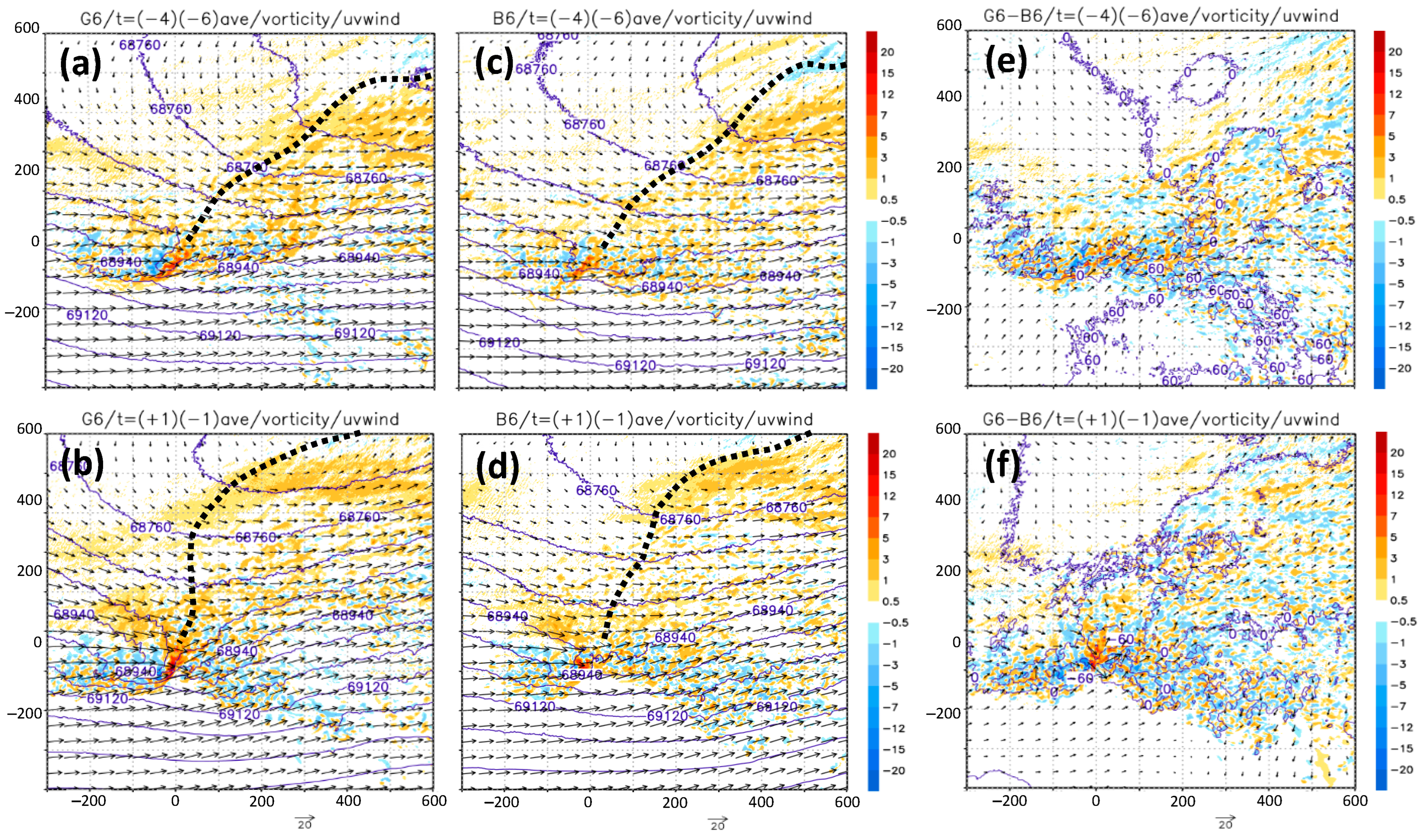
For the level of z = 3201 m (near 700 hPa) farther up, Figure 12 shows the composites of pressure, relative vorticity, and wind fields for GMs, BMs, and their differences at P1 and P3 over the same square domain. At this level, the bow echo in the GM composites is seen to develop near the base of the trough, and its protruding leading line is mostly associated with positive vorticity (warm colors) following P1 (Figure 12a). Behind the line, relative vorticity is mostly negative (cold colors) within about 30–40 km. When the bow echo becomes the most evident at P3 (Figure 12b), the northern half on its backside becomes dominated by positive vorticity, whereas the southern half is dominated by negative vorticity, consistent with the development of a pair of bookend vortices and the intensification of the RIJ [1,3,6,7,8,17,18,19,20,21,22,23,24,25]. Similar to Figure 11, the convective line in BMs also exhibits a weaker signature in relative vorticity and its associated trough is not as deep (Figure 12c,d), which is likely a reflection of a weaker overall latent heating effect near the bow echo. Although the rear inflow in the BM group is not as strong, the positive–negative vorticity pair is still present at the backside at P3 (Figure 12d). From their differences, one can also see that near 700 hPa, the westerly rear inflow and the prevailing southwesterly flow to the south of the system are both stronger in GMs compared to BMs (Figure 12e,f).
Figure 12.
As in Figure 11 but showing pressure (Pa, isobars every 0.6 hPa), relative vorticity (10−4 s−1, color, scale to the right of middle column), and horizontal wind vectors (m s−1, reference length at bottom) at z = 3201 m in the GM group at (a) P1 and (b) P3; those in the BM group at (c) P1 and (d) P3; and (e,f) their differences (GM minus BM).
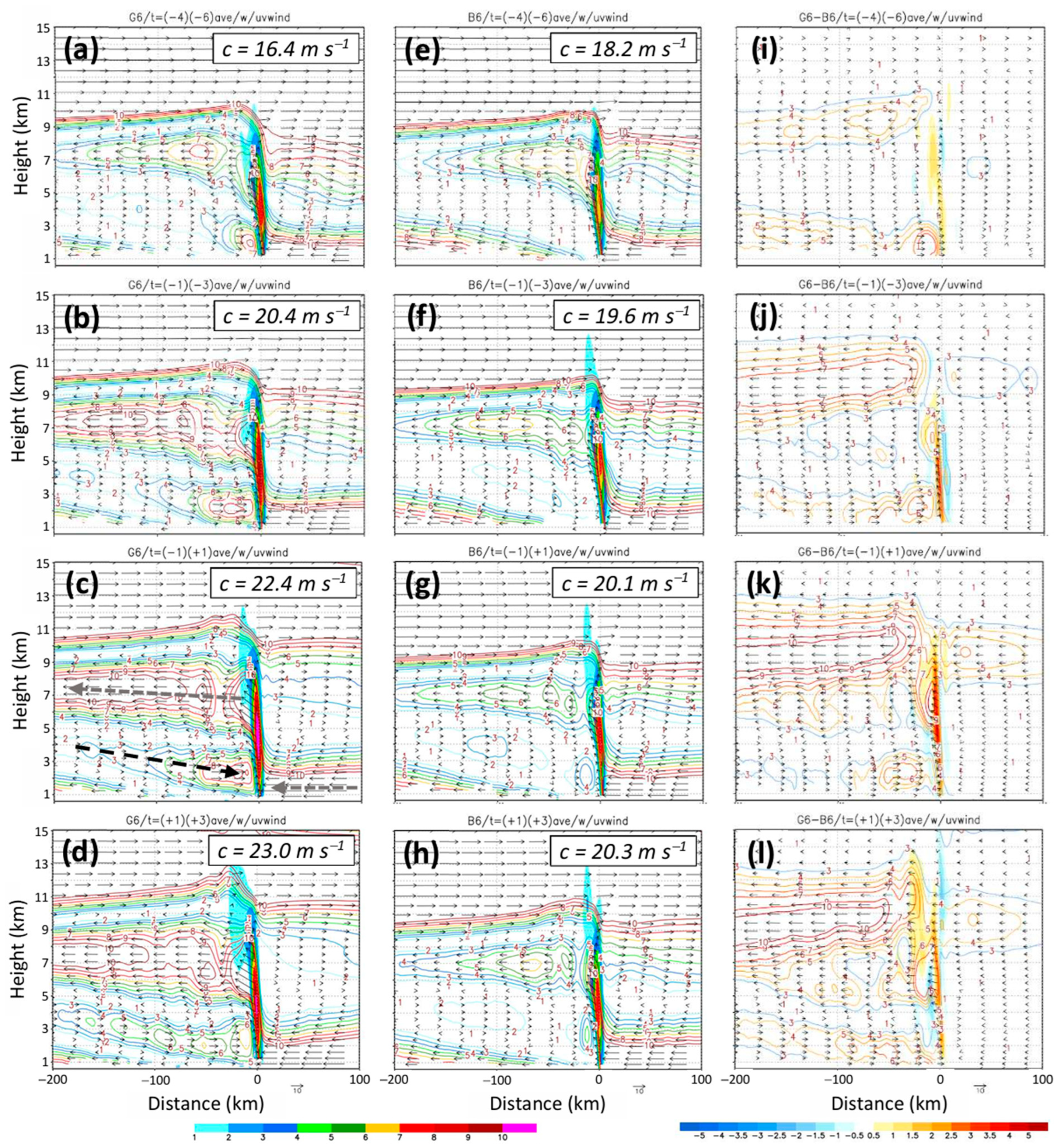
Figure 13 compares the kinematic structure of the bow echo in the GM and BM groups on the vertical cross-section, along the axis of the RIJ, and through the bow apex, from 200 km behind to 100 km ahead of the apex. Following stage P1, the tilted updraft at the leading edge in the GM composite is stronger than BMs, especially evident at the lower and middle troposphere, despite its initial slower propagation speed (Figure 13, top row). Linked to this stronger updraft, the system-relative FTR outflow behind the updraft also appears thicker in depth and extends higher in elevation, peaking at about z = 7.5 km in GMs (versus ~7.0 km in BMs). At this stage, the system-relative RIJ in GMs has already appeared at the immediate backside of the leading line below 4–5 km, but there is little sign for its existence in BMs. These differences are also reflected in the panel of GM minus BM. As the bow echo in GMs strengthens in P2 and P3, it starts to propagate at a speed over 20 m s−1, faster than the system in BMs, consistent with its stronger RIJ that exceeds 9–10 m s−1 (compared to about 3–4 m s−1 in BM), and extends much farther back behind the line (rows 2 and 3 in Figure 13). Thus, at P3, the RIJ in GMs has a maximum ground speed of close to 30 m s−1. The FTR outflow aloft that corresponds to the stratiform region in GMs now becomes stronger and deeper as well. As a result, in the difference plots, the GM updraft is much stronger and more buoyant, as are the upper-level FTR outflow, roughly over z = 7–15 km, and the RIJ, by more than 6 m s−1 right behind the line near z = 2–2.5 km (Figure 13j,k). At P4, the bow echo in GMs reaches its highest moving speed of 23 m s−1 (Figure 13d), faster than the BM system by 2.7 m s−1 (Figure 13h), with similar differences (Figure 13l). At this stage, the RIJ in GMs also has descended closer to the surface due to its negative buoyancy. Similar differences continue into P5 but become smaller. Also, because the RIJ in GMs is considerably stronger and extends much farther back, it is able to draw in drier mid-level air from the environment than that in BMs, with lower equivalent potential temperatures (θe) by about 1 K in the RIJ at P3, resulting in a stronger cold pool by about 2 K behind the leading edge at/near the surface as well. This combination of a stronger RIJ, cold pool, and updraft is helpful in maintaining the intensity of the bow echo, as reviewed in Section 1, e.g., [3,6,7,8,17,18,19,20,21,22]. Next, in the following section, we further explore and discuss the reasons for such differences to occur in the environment.
Figure 13.
Composite vertical cross-sections along the direction of the RIJ and through the apex of the bow echo of the GM group, showing system-relative velocity vectors (all in m s−1), wind speed (color contours, every 1 m s−1 from 1 to 10 m s−1), and vertical velocity (w, color shades) on the section plane at (a) P1 to (d) P4. The reference vector length and color scale are both plotted below the bottom panel. (e–h) are the same as in (a–d), except in the BM group, and (i–l) their differences (GM minus BM, scale at bottom) at the four phases. The length of the cross-sections is 300 km (apex located at the origin), with the distance increasing in the direction of system propagation. The average moving speed of the group is given inside each panel.
4. Discussion
In this section, our focus is to find the answers to the question: what are the environmental factors leading to the differences in the intensity and morphology of bow echoes in the ensemble simulations? As four of the GMs are produced using NCEP FNL as IC/LBCs while four of the BMs are using the JMA GANAL (Table 3), differences must exist in the environment contained in these two datasets that lead to, or at least contribute to, the different outcomes in CReSS simulations. Therefore, we compare their differences at key instances during the lifespan of the bow echo at 0600 UTC 12 April, when the CI is about to occur within a few hours, and at 1800 UTC 12 April, when the bow echo intensifies toward its maximum intensity (see Table 4).
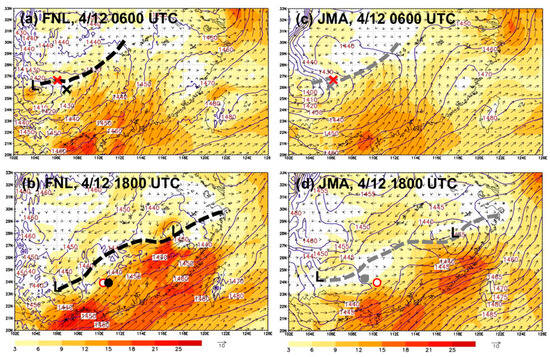
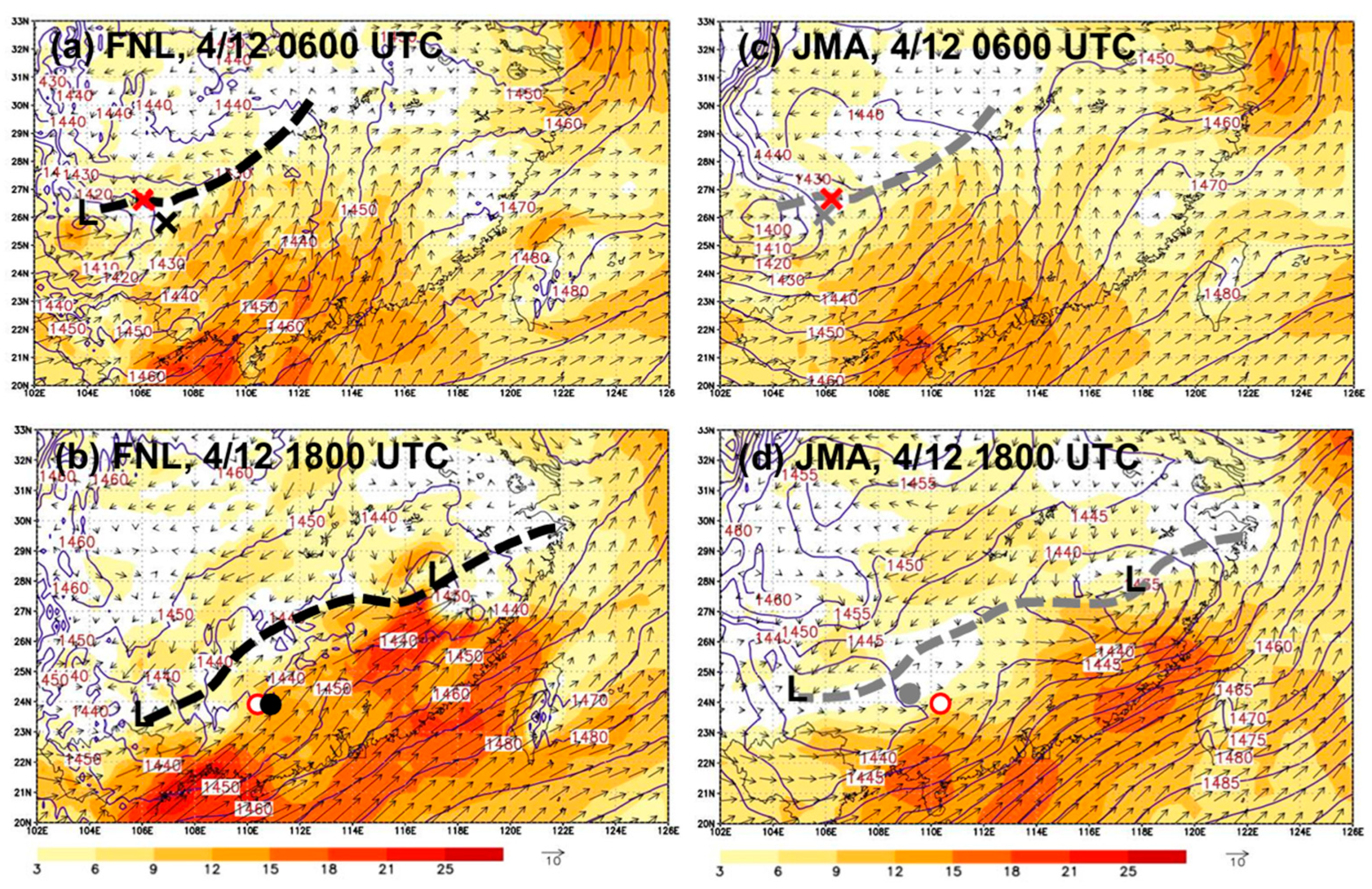
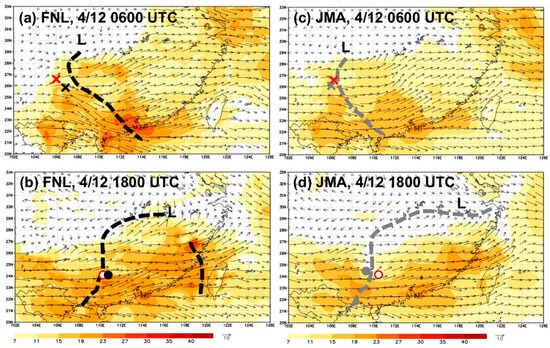
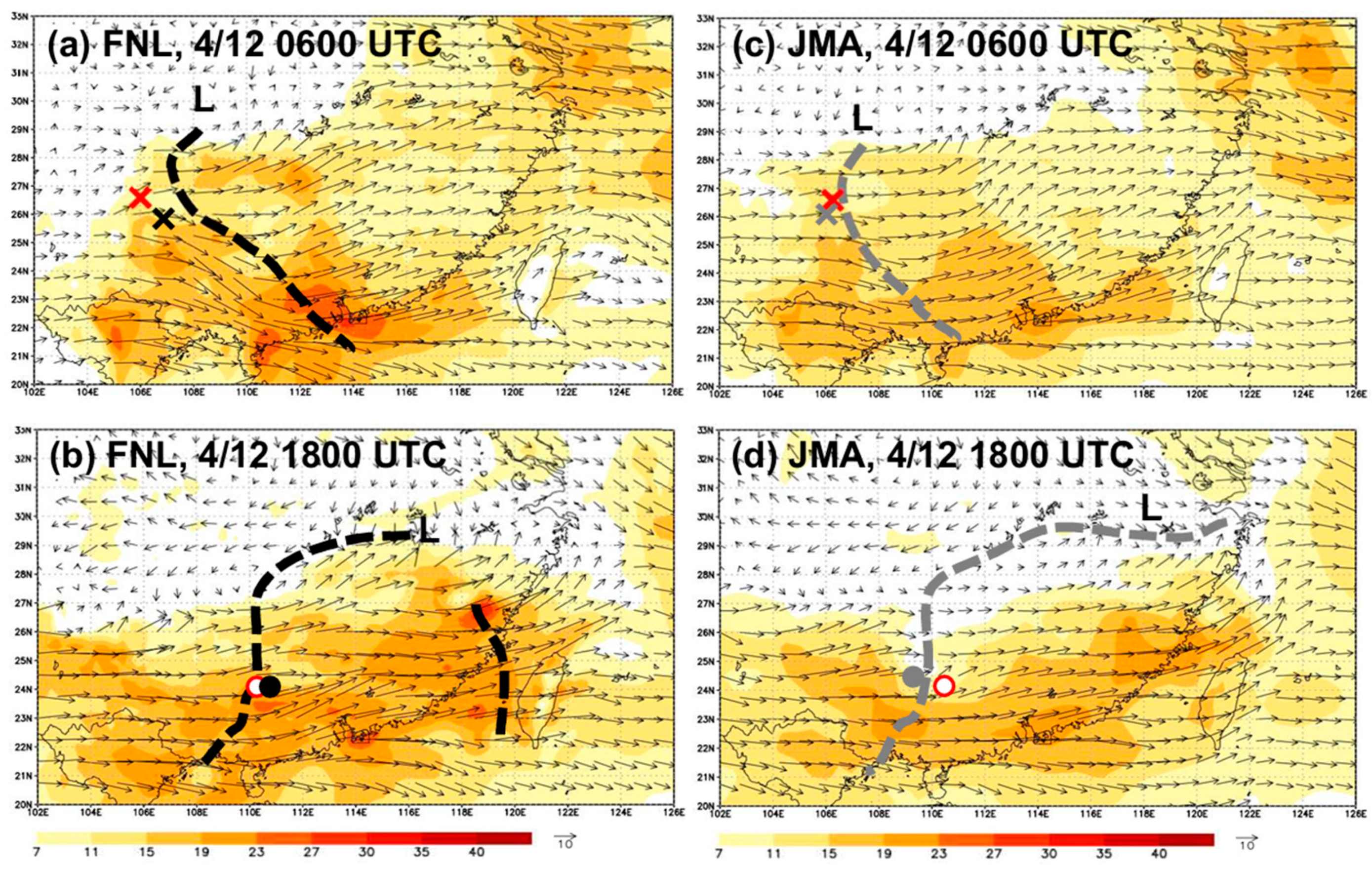
Figure 14 compares the height and wind fields at 850 hPa between NCEP FNL and JMA analyses, which for the FNL at 1800 UTC is the same as Figure 10e but at a different level. While the locations of the 850 hPa trough are similar in the two datasets at both times, the southwesterly flow on the warm side is overall stronger in the NCEP FNL compared to JMA. At 0600 UTC, the difference in the southwesterly flow is quite evident near the location of CI (Figure 14a,c). Also, on average, the CI in GMs occurs farther to the east, making it closer to the stronger southwesterly winds in the FNL (reaching about 10 m s−1). At 1800 UTC, the differences in southwesterly wind speed between the two datasets over the pre-frontal region are further enlarged, especially near the frontal zone (Figure 14b,d). Due to the faster propagation speed of the bow echo and its location farther to the east in GMs, the environmental flow (and thus, the low-level FTR inflow feeding into the system) is also significantly stronger in GMs (about 12 m s−1) at 850 hPa compared to BMs (≤3 m s−1), leading to its stronger updraft. This is a distinct difference between the two datasets and the two groups. A similar difference in the strength of the low-level southerly flow was found in a heavy-rainfall event in South China [36].
Figure 14.
Comparisons of 850 hPa geopotential height (gpm, contours every 10 gpm) and wind vectors and speeds (m s−1, speed in color, with color scale and vector reference length at bottom) in NCEP FNL analysis at (a) 0600 and (b) 1800 UTC 12 April 2016. (c,d) are the same as in (a,b), except for JMA GANAL. Thick dashed lines indicate trough. Red, black, and gray “x” symbols in (a,c) mark the observed location, average location in GMs, and average location in BMs of CI (exact time not at 0600 UTC). Similarly, red open circle, black dot, and gray dot in (b,d) mark the observed location of bow apex, and the average locations in GMs and BMs at 1800 UTC.
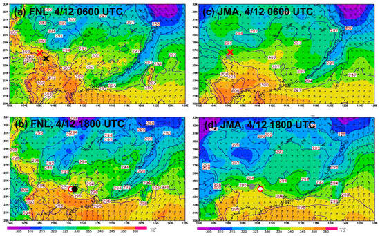
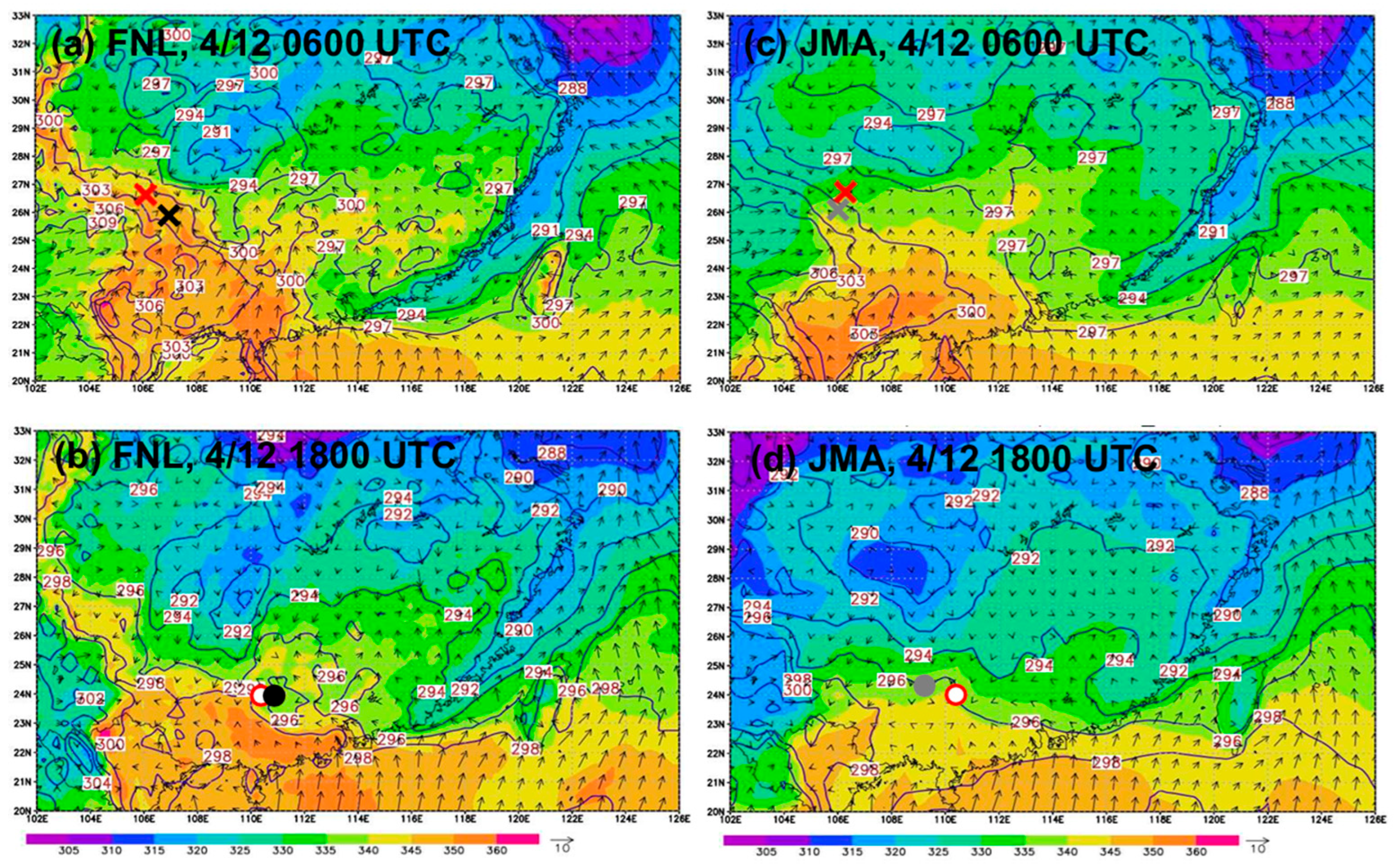
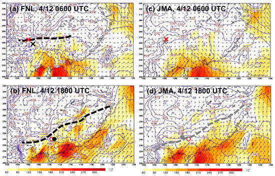
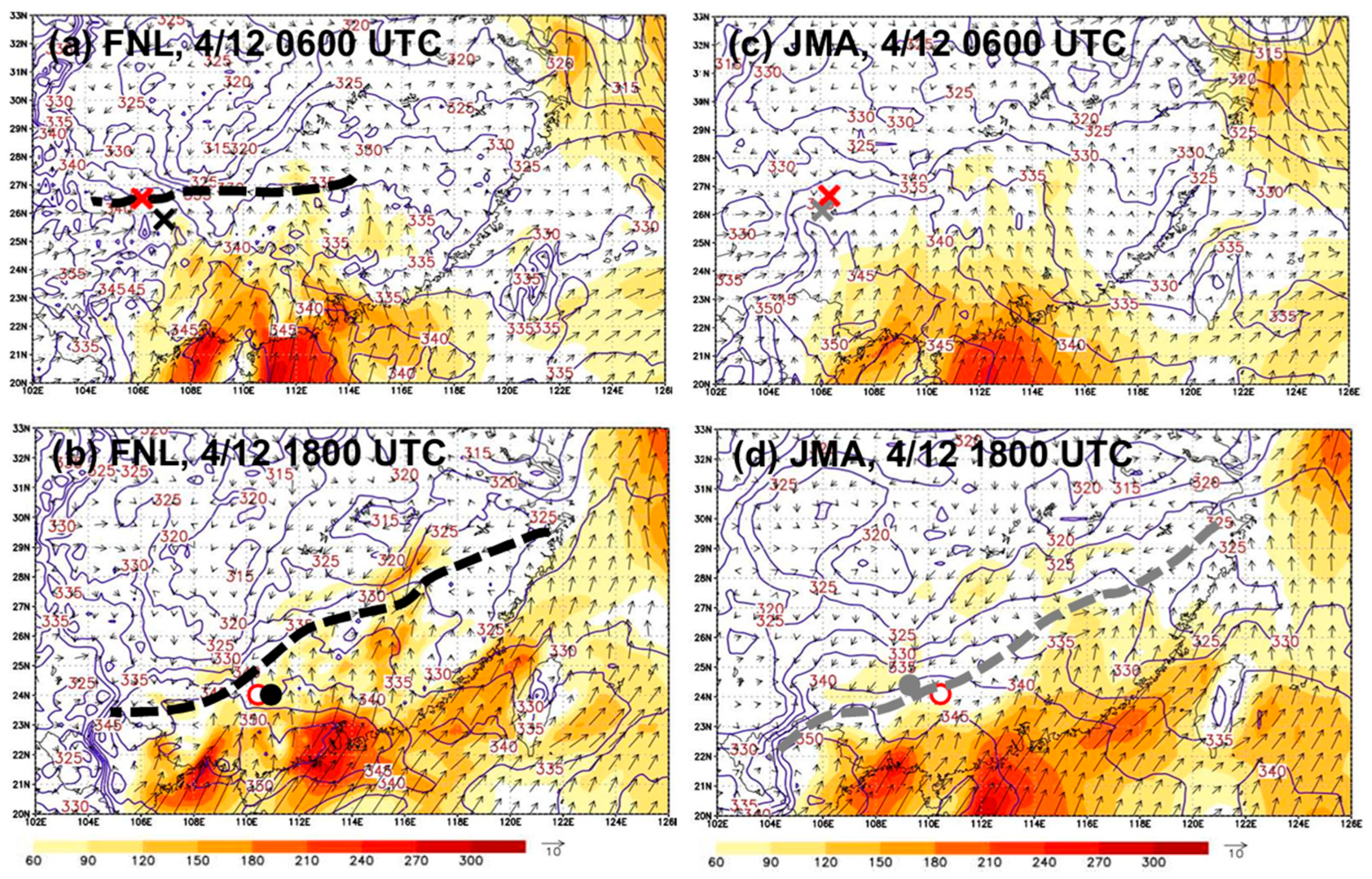
The environmental conditions at 1000 and 925 hPa closer to the surface in the two datasets are shown in Figure 15 and Figure 16. Clearly linked to the stronger southwesterly flow and advection, the FNL fields are warmer and moister, with higher θe values near the convective system than the JMA fields at both 0600 and 1800 UTC 12 April. At 0600 UTC, the θe at the CI location is at least 5 K higher in the FNL (~348 K) than the JMA (~340 K) at 1000 hPa (Figure 15a,c). As the bow echo strengthens at 1800 UTC (Figure 15b,d), the near-surface air feeding into the system also has significantly higher θe values (reaching ≥350 K) in FNL, due to its proximity to the warmer and wetter region, than the JMA data (θe ≈ 340 K). Thus, at 925 hPa near the surface, the moisture flux in terms of mixing ratio is also stronger just upstream of the system in the FNL at both times (Figure 16), particularly at 1800 UTC when the bow echo is propagating faster and farther ahead of the trough, into the warmer and moister environment. At this time, the moisture flux just to the south of the bow echo can reach 120 g kg−1 m s−1 in the FNL (Figure 16b), twice as large compared to only about 60 g kg−1 m s−1 in the JMA (Figure 16d). Therefore, the GM bow echoes are more robust and possess a stronger and more buoyant updraft that reaches higher into the upper troposphere, as seen in Figure 13. In some earlier studies over South China, the model results were also found to be sensitive to moisture amount in the initial field, e.g., [35].
Figure 15.
Similar to Figure 14, but showing 1000 hPa temperature (K, isotherms every 3 K), θe (K, color, scale at bottom), and wind vectors (m s−1, reference length at bottom) in FNL and JMA at the two times (as labeled). The trough location is not plotted.
Figure 16.
Similar to Figure 14, but showing 925 hPa water vapor flux (g kg−1 m s−1, color, scale at bottom), θe (K, purple contours every 5 K), and wind vectors (m s−1, reference length at bottom) in FNL and JMA. Thick dashed lines indicate trough/wind-shift line.
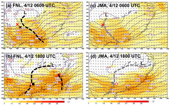
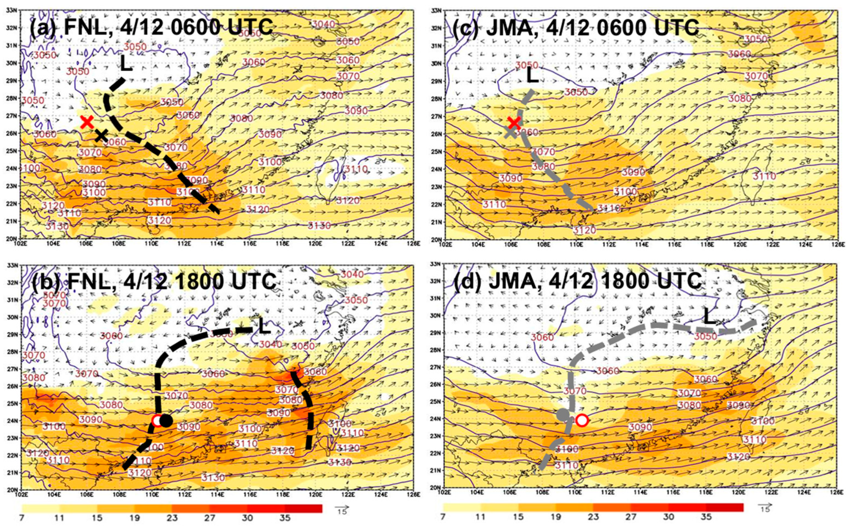
The conditions in the NCEP FNL and JMA GANAL at 700 hPa are compared in Figure 17. As mentioned earlier (see Figure 12), the FNL data provide a stronger westerly flow at this level behind the trough over the region of CI at 0600 UTC 12 April compared to the JMA (Figure 17a,c). Even more evident at 0000 UTC, this difference is maintained through 1800 UTC (Figure 17b,d), when the bow echo in GMs has propagated faster to a location slightly ahead of the 700 hPa trough, whereas the system in BMs still lags behind its corresponding trough. As a result, the 1000–700 hPa vertical wind shear at 0600 UTC over the CI region, pointing toward the southeast, is also stronger in the FNL (about 17 m s−1, Figure 18a) versus the JMA (about 13 m s−1, Figure 18c). Likewise, at 1800 UTC, the low-level vertical shear is also stronger in the FNL (about 20–21 m s−1, Figure 18b) compared to the JMA (about 10 m s−1, Figure 18d), even though it is now pointing toward the east or slightly east–southeast near the bow echo. Thus, conditions in the low-to-mid-level wind and vertical wind shear also differed between the NCEP FNL and JMA GANAL during the lifespan of the bow echo. In the former dataset, the stronger 700 hPa wind increases the momentum supply and contributes toward a stronger RIJ associated with the system, and its stronger vertical wind shear, coupled with a stronger pair of updraft and downdraft (Figure 13), also promotes system intensity in terms of the bookend vortices and thus the RIJ through the tilting effect, as reviewed in Section 1 [1,6,7,8,19,20,21,22,23,24,25].
Figure 17.
Similar to Figure 14, but at 700 hPa in (a,b) NCEP FNL and (c,d) JMA GANAL at the two times.
Figure 18.
Similar to Figure 17, but showing the vertical wind shear vectors (m s−1) over the layer of 1000–700 hPa in (a,b) NCEP FNL and (c,d) JMA GANAL at the two times.
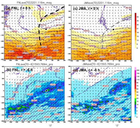
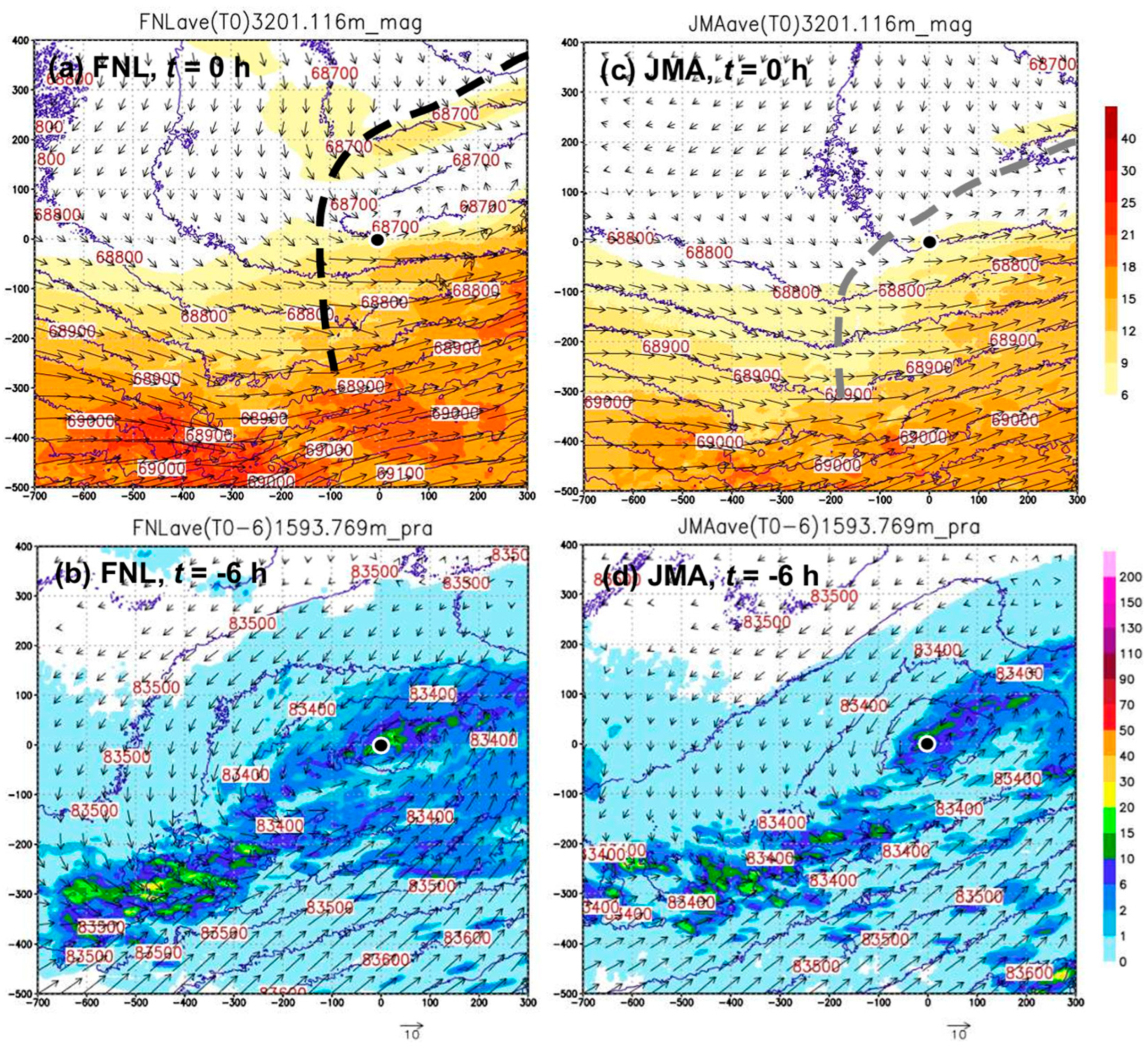
In Figure 19, we present the composite pressure and wind fields at z = 3201 m while at t = 0 h (Table 4), and hourly rainfall distributions ending at t = −6 h, of the FNL and JMA members, instead of in the analyses. At the maturation stage, the FNL members produce a deeper trough with significantly stronger westerly flow, providing stronger westerly wind shear and consistent with earlier discussion (Figure 19a,c). Note that at this level, the northwesterly flow at the backside of the bow echo (apex located at the origin) is also much stronger and contributing to the RIJ in the FNL members. This is consistent with the stronger trough, with much more abundant hourly rainfall in these members before t = −6 h several hours earlier (Figure 19b,d). As also shown in Figure 11, this difference in rainfall is persistent throughout the lifecycle of the bow echo, including the region to its northeast, where the low pressure near 850 hPa exists. Thus, as part of the circulation associated with the low pressure (see Figure 11), the northwesterly flow behind the bow echo, i.e., its RIJ, is also strengthened through this mechanism. Overall, through the interactions among warmer, moister, and stronger winds with larger vertical wind shear at low levels, the pair of updraft/downdraft in the GM group (mostly using FNL as IC/LBCs) becomes stronger, leading to stronger RIJ that extends farther back behind the system, and thus, a more distinct bulge of the bow echo as well as its faster propagation speed and longer duration.
Figure 19.
(a) Composite pressure (Pa, isobars every 50 Pa) and horizontal wind vectors (m s−1, reference length at bottom) and speed (m s−1, color) at t = 0 h (i.e., mid-point of P3, see Table 4), all at z = 3201 m; and (b) composite pressure, wind vectors at t = −6 h and z = 1594 m, and hourly rainfall (mm, color) prior to t = −6 h in FNL members. (c,d) are the same as in (a,b), but from JMA members. For both wind speed and hourly rainfall, the color scales are plotted to the far right. The domain shown is 1000 km × 900 km in size, and the apex is located at (0, 0) marked by a black dot. Thick dashed lines (a,c) indicate the trough/wind-shift line.
Finally, it should be noted that even with more favorable conditions in the environment, not all CReSS experiments using the NCEP FNL analyses were good members, and likewise, not all runs using JMA data belong to BMs (Table 3). This implies some uncertainty among the ensemble experiments exists. Perhaps, the ensemble-based sensitivity analysis, e.g., [63,64], similar to [56], can be applied for a more quantitative assessment in the future. Also, although in agreement with [30] to some extent, our results herein are based on a single bow-echo case, and thus, have limitations and only apply to similar scenarios.
5. Conclusions
This study investigates the development and evolution of a long-lived bow echo in South China over 12–13 April 2016 using a series of 20 high-resolution ensemble experiments with the CReSS model at a horizontal grid size of Δx = 2 km. Synoptic and thermodynamic analyses showed that this system developed near a surface front under favorable conditions, with dynamic uplifting ahead of approaching troughs at 500 and 700 hPa and instability with a fair amount of CAPE (~850 J kg−1). After formation, the bow echo propagated at a speed of over 20 m s−1 toward the east–southeast across South China and stayed ahead of the 850 hPa front, which was also deepening with a low-pressure center developing to the northeast of the bow echo. The ensemble was produced by using four different gridded analysis datasets from the United States, Europe, and Japan as IC/LBCs, combined with five different initial times 6 h apart.
Deemed to be the best in the ensemble, the CTRL successfully reproduced the development and evolution of the bow echo in agreement with the above analysis. Various signature components of the bow echo in their structure and kinematic field were also well captured in the CTRL, including tilted updraft/downdraft pairs, system-relative inflows and outflows, RIJs, and bookend vortices. In the other 19 experiments, the morphology and evolution of the bow echo were reproduced at various levels of success, and the six best-performing members were chosen as “good members” (the GM group), and the six worst ones were chosen as “bad members” (the BM group). By comparing the two groups, it is determined that a stronger bow echo with a more distinct protruding bulge in this event is associated with a stronger and more buoyant updraft, a thicker stratiform region that also extends higher in elevation, more overall rainfall, a stronger RIJ that extends farther back in distance (and thus the downdraft), more distinct bookend vortices, and a stronger cold pool (and the gust front), thereby resulting in a faster propagation speed, an increased severity, and a longer lifespan of the system. In the BM group, all the above features are weaker and the MCS shorter in duration.
By comparing the NCEP FNL analysis that fostered four of the six GMs (including CTRL) with the JMA GANAL, which produced four BMs, several environmental factors that contributed to a more intense and longer-lived bow echo in the CReSS experiments have also been identified, as listed below:
- A stronger and moister low-level southwesterly flow to the south of the front to produce a stronger moisture flux and convergence at the leading edge, with higher θe values (by ≥5 K) and a stronger FTR inflow feeding into the bow echo, leading to the significantly stronger and taller updraft, and overall more abundant hydrometeors and rainfall;
- A stronger northwesterly to westerly wind near 700 hPa and thus stronger 1000–700 hPa vertical wind shear (almost twice as strong), causing a stronger RIJ behind the apex, a bookend vortex pair that focuses and reinforces the RIJ, and, eventually, a faster propagation speed;
- A deeper low near 850 hPa along the front with a center to the northeast of the bow echo, associated with more rainfall and latent heating, where its circulation can feed into the backside of the bow echo with low θe air, further strengthening the RIJ and cold pool;
- A CI location farther to the east due to more favorable conditions with higher θe given in point 1, which in turn contributes to the strength of the updraft and thus the severity of the storm, as well as a faster speed to keep staying in the more favorable environment.
Because in a severe storm such as a bow echo, the updraft/downdraft can reinforce each other, while all the above points are inter-connected through interaction, as reviewed in Section 1. As pointed out here, several favorable conditions in the environment co-existed in the present case, including in the vertical wind shear, low-level convergence and moisture supply, instability, and the strength of the RIJ once the system formed, leading to the development of the current bow echo with a long lifespan of 15 h in South China.
Author Contributions
Conceptualization, C.-C.W. and Z.M.; methodology, C.-C.W. and C.-C.H.; software, C.-C.H., Y.-H.C. and K.T.; validation, C.-C.W. and C.-C.H.; formal analysis, C.-C.W., C.-C.H. and Y.-H.C.; investigation, C.-C.W., C.-C.H. and Y.-H.C.; resources, C.-C.W., Z.M. and K.T.; data curation, C.-C.H. and K.T.; writing—original draft preparation, C.-C.W., C.-C.H. and Y.-H.C.; writing—review and editing, all authors; visualization, C.-C.H.; supervision, C.-C.W.; project administration, C.-C.W.; funding acquisition, C.-C.W. and Z.M. All authors have read and agreed to the published version of the manuscript.
Funding
This research was funded by the National Science and Technology Council (NSTC) of Taiwan, under grants NSTC 114-2111-M-003-004 and NSTC 114-2625-M-003-004, including the APC.
Institutional Review Board Statement
Not applicable.
Informed Consent Statement
Not applicable.
Data Availability Statement
The CReSS model and its user’s guide are open to researchers and available at http://www.rain.hyarc.nagoya-u.ac.jp/~tsuboki/cress_html/index_cress_eng.html (accessed on 13 October 2017). The analysis datasets used in this study are open and available at http://rda.ucar.edu/datasets/ds335.0/#!description (NCEP GFS FNL, accessed on 14 January 2018), http://nomads.ncep.noaa.gov/pub/data/nccf/com/cfs/prod/ (NCEP GFSv2, accessed on 3 July 2018), https://cds.climate.copernicus.eu/stac-browser/collections/reanalysis-era-interim (ECMWF ERA-Interim, accessed on 10 April 2018), and https://www.wis-jma.go.jp/cms/gsm/download.html (JMA GANAL, accessed on 12 December 2018).
Acknowledgments
The National Center for High-Performance Computing (NCHC) in Taiwan is acknowledged for providing computation resources for this study. We also thank the assistance of Chih-Sheng Chang during manuscript preparation.
Conflicts of Interest
The authors declare no conflicts of interest.
Abbreviations
The following abbreviations are used in this manuscript:
| BM | Bad Member |
| CAPE | Convective Available Potential Energy |
| CFSv2 | Climate Forecast System Version 2 |
| CI | Convective Initiation |
| CIN | Convective Inhibition |
| CReSS | Cloud-Resolving Storm Simulator |
| CWA | Central Weather Administration |
| CTRL | Control Experiment |
| ECMWF | European Center for Medium-Range Weather Forecast |
| ERA | ECMWF Reanalysis |
| FTR | Front-to-Rear |
| GANAL | Global Spectral Model Analysis |
| GFS | Global Forecast System |
| GM | Good Member |
| IC/LBCs | Initial and Lateral Boundary Conditions |
| JMA | Japan Meteorological Agency |
| MCS | Mesoscale convective system |
| NCEP | National Centers for Environmental Prediction |
| NOAA | National Oceanic and Atmospheric Administration |
| RIJ | Rear Inflow Jet |
| RTF | Rear-to-Front |
| SST | Sea Surface Temperature |
References
- Fujita, T.T. Manual of Downburst Identification for Project NIMROD; Satellite and Mesometeorology Research Paper No.156; Department of Geosciences, University of Chicago: Chicago, IL, USA, 1978; 104p. [Google Scholar]
- Johns, R.H.; Hirt, W.D. Derechos: Widespread convectively induced wind-storms. Weather Forecast. 1987, 2, 32–49. [Google Scholar] [CrossRef] [Scilit]
- Przybylinski, R.W. The bow echo: Observations, numerical simulations, and severe weather detection methods. Weather Forecast. 1995, 10, 203–218. [Google Scholar] [CrossRef] [Scilit]
- Burgess, D.W.; Ray, P.S. Principle of Radar. In Mesoscale Meteorology and Forecasting; Ray, P.S., Ed.; American Meteorological Society: Boston, MA, USA, 1986; pp. 85–117. [Google Scholar]
- Nolen, R.H. A radar pattern associated with tornadoes. Bull. Am. Meteorol. Soc. 1959, 40, 277–279. [Google Scholar] [CrossRef] [Scilit]
- Weisman, M.L. The genesis of severe, long-lived bow echoes. J. Atmos. Sci. 1993, 50, 645–670. [Google Scholar] [CrossRef] [Scilit]
- Weisman, M.L. Bow echoes: A tribute to T. T. Fujita. Bull. Am. Meteorol. Soc. 2001, 82, 97–116. [Google Scholar] [CrossRef] [Scilit]
- Davis, C.; Atkins, C.; Bartels, D.; Bosart, L.; Coniglio, M.; Bryan, G.; Cotton, W.; Dowell, D.; Jewett, B.; Johns, R.; et al. The Bow Echo and MCV Experiment. Observations and opportunities. Bull. Am. Meteorol. Soc. 2004, 85, 1075–1093. [Google Scholar] [CrossRef] [Scilit]
- Wakimoto, R.M. The West Bend Wisconsin storm of 4 April 1981: A problem in operational meteorology. J. Clim. Appl. Meteorol. 1983, 22, 181–189. [Google Scholar] [CrossRef] [Scilit]
- Johns, R.H. Meteorological conditions associated with bow echo development in convective storms. Weather Forecast. 1993, 8, 294–299. [Google Scholar] [CrossRef] [Scilit]
- Johns, R.H.; Howard, K.W.; Maddox, R.A. Conditions associated with long-lived derechos—An examination of the large-scale environment. In 16th Conference on Severe Local Storms, Kananaskis Park, AB, Canada; American Meteorological Society: Boston, MA, USA, 1990; pp. 408–412. [Google Scholar]
- Smull, B.F.; Houze, R.A., Jr. A midlatitude squall line with a trailing region of stratiform rain: Radar and satellite observations. Mon. Weather Rev. 1985, 113, 117–133. [Google Scholar] [CrossRef] [Scilit]
- Houze, R.A., Jr.; Rutledge, S.A.; Biggerstaff, M.I.; Smull, B.F. Interpretation of Doppler radar displays of mid-latitude mesoscale convective systems. Bull. Am. Meteorol. Soc. 1989, 70, 608–619. [Google Scholar] [CrossRef] [Scilit]
- Funk, T.W.; Darmofal, K.E.; Kirkpatrick, J.D.; DeWald, V.L.; Przybylinski, R.W.; Schmocker, G.K.; Lin, Y.-J. Storm reflectivity and mesocyclone evolution associated with the 15 April 1994 squall line over Kentucky and southern Indiana. Weather Forecast. 1999, 14, 976–993. [Google Scholar] [CrossRef] [Scilit]
- Rotunno, R.; Klemp, J.B.; Weisman, M.L. A theory for strong, long-lived squall line. J. Atmos. Sci. 1988, 45, 463–485. [Google Scholar] [CrossRef] [Scilit]
- Skamarock, W.C.; Weisman, M.L.; Klemp, J.B. Three-dimensional evolution of simulated long-lived squall lines. J. Atmos. Sci. 1994, 51, 2563–2584. [Google Scholar] [CrossRef] [Scilit]
- Smull, B.F.; Houze, R.A., Jr. Rear inflow in squall-lines with trailing stratiform precipitation. Mon. Weather Rev. 1987, 115, 2869–2889. [Google Scholar] [CrossRef] [Scilit]
- Braun, S.A.; Houze, R.A., Jr. The evolution of the 10–11 June 1985 PRE-STORM squall line: Initiation, development of rear inflow, and dissipation. Mon. Weather Rev. 1997, 125, 478–504. [Google Scholar] [CrossRef] [Scilit]
- Weisman, M.L. The role of convectively generated rear-inflow jets in the evolution of long-lived mesoconvective systems. J. Atmos. Sci. 1992, 49, 1826–1847. [Google Scholar] [CrossRef] [Scilit]
- Atkins, N.T.; Arnott, J.M.; Przybylinski, R.W.; Wolf, R.A.; Ketcham, B.D. Vortex structure and evolution within bow echoes. Part I: Single-Doppler and damage analysis of the 29 June 1998 derecho. Mon. Weather Rev. 2004, 132, 2224–2242. [Google Scholar] [CrossRef] [Scilit]
- Lee, W.-C.; Wakimoto, R.M.; Carbone, R.E. The evolution and structure of a “bow-echo-microburst” event. Part II: The bow echo. Mon. Weather Rev. 1992, 120, 2211–2225. [Google Scholar] [CrossRef] [Scilit]
- Houze, R.A., Jr. 100 Years of research on mesoscale convective systems. Meteorol. Monogr. 2018, 59, 17.1–17.54. [Google Scholar] [CrossRef] [Scilit]
- Weisman, M.L.; Davis, C. Mechanisms for the generation of mesoscale vortices within quasi-linear convective systems. J. Atmos. Sci. 1998, 55, 2603–2622. [Google Scholar] [CrossRef] [Scilit]
- Weisman, M.L.; Trapp, R.J. Low-level mesovortices within squall lines and bow echoes. Part I: Overview and dependence on environmental shear. Mon. Weather Rev. 2003, 131, 2779–2803. [Google Scholar] [CrossRef] [Scilit]
- Atkins, N.T.; Laurent, M.S. Bow echo mesovortices. Part II: Their genesis. Mon. Weather Rev. 2009, 137, 1514–1532. [Google Scholar] [CrossRef] [Scilit]
- Li, J.; Geiss, A.; Feng, Z.; Leung, L.R.; Qian, Y.; Cui, W. A derecho climatology (2004–2021) based on machine learning identification of bow echoes. Earth Syst. Sci. Data 2025, 17, 3721–3745. [Google Scholar] [CrossRef] [Scilit]
- Meng, Z.; Zhang, F.; Markowski, P.; Wu, D.; Zhao, K. A modeling study on the development of a bowing structure and associated rear inflow within a squall line over South China. J. Atmos. Sci. 2012, 69, 1182–1207. [Google Scholar] [CrossRef] [Scilit]
- Meng, Z.; Yan, D.; Zhang, Y. General features of squall lines in East China. Mon. Weather Rev. 2013, 141, 1629–1647. [Google Scholar] [CrossRef] [Scilit]
- Qi, L.Y.; Chen, Y.; Ye, L.B.; Nong, M.S. Characteristics of bow echoes during 2011–2020 in western South China. J. Trop. Meteor. 2024, 30, 428–443. [Google Scholar] [CrossRef] [Scilit]
- Liu, Q.; Xu, X.; Zhao, K.; Zhou, A. A merger-formation bow echo caused by low-level mesovortex in South China. J. Geophys. Res. Atmos. 2023, 128, e2022JD037954. [Google Scholar] [CrossRef] [Scilit]
- Xu, C.; Zhang, L.; Xiao, X. Evolution characteristics and mechanism of meso-γ-scale vortex in an atypical bow echo in the North China Plain. Atmos. Res. 2024, 311, 107657. [Google Scholar] [CrossRef] [Scilit]
- Liu, Q.; Zhou, A.; Zhao, K.; Xu, X.; Huang, H. Microphysical evolution of heavy rainfall during a bow echo event in South China. J. Geophys. Res. Atmos. 2025, 130, e2024JD041381. [Google Scholar] [CrossRef] [Scilit]
- Chen, G.T.-J.; Wang, C.-C.; Chou, H.-C. Case study of a bow echo near Taiwan during wintertime. J. Meteorol. Soc. Jpn. 2007, 85, 233–253. [Google Scholar]
- Wang, C.-C.; Hou, J.-P.; Tseng, C.-H.; Chang, P.-L.; Lee, D.-I. Study of an asymmetric and anticyclonic bow echo near Taiwan. Atmosphere 2022, 13, 331. [Google Scholar] [CrossRef] [Scilit]
- Wu, D.; Meng, Z.; Yan, D. The predictability of a squall line in South China on 23 April 2007. Adv. Atmos. Sci. 2013, 30, 485–502. [Google Scholar] [CrossRef] [Scilit]
- Wu, N.; Zhuang, X.; Min, J.; Meng, Z. Practical and intrinsic predictability of a warm-sector torrential rainfall event in the South China monsoon region. J. Geophys. Res. 2022, 125, e2019JD031313. [Google Scholar] [CrossRef] [Scilit]
- Kalnay, E.; Kanamitsu, M.; Baker, W.E. Global numerical weather prediction at the national meteorological center. Bull. Am. Meteorol. Soc. 1990, 71, 1410–1428. [Google Scholar] [CrossRef] [Scilit]
- Kleist, D.T.; Parrish, D.F.; Derber, J.C.; Treadon, R.; Wu, W.S.; Lord, S. Introduction of the GSI into the NCEP global data assimilation system. Weather Forecast. 2009, 24, 1691–1705. [Google Scholar] [CrossRef] [Scilit]
- Saha, S.; Moorthi, S.; Wu, X.; Wang, J.; Nadiga, S.; Tripp, P.; Behringer, D.; Hou, Y.-T.; Chuang, H.-Y.; Iredell, M.; et al. The NCEP Climate Forecast System version 2. J. Clim. 2014, 27, 2185–2208. [Google Scholar] [CrossRef] [Scilit]
- Berrisford, P.; Dee, D.P.; Poli, P.; Brugge, R.; Fielding, K.; Fuentes, M.; Kållberg, P.W.; Kobayashi, S.; Uppala, S.; Simmons, A. The ERA-Interim Archive Version 2.0. ERA Report, ECMWF, 2011, 23p. Available online: https://www.ecmwf.int/en/elibrary/8174-era-interimarchive-version-20 (accessed on 18 March 2026).
- Dee, P.D.; Uppala, S.M.; Simmons, A.J.; Berrisford, P.; Poli, P.; Kobayashi, S.; Andrae, U.; Balmaseda, M.A.; Balsamo, G.; Bauer, P.; et al. The ERA-Interim reanalysis: Configuration and performance of the data assimilation system. Q. J. R. Meteorol. Soc. 2011, 137, 553–597. [Google Scholar] [CrossRef] [Scilit]
- Tsuyuki, T.; Fujita, T. (Eds.) Outline of the Operational Numerical Weather Prediction at the Japanese Meteorological Agency; JMA: Tokyo, Japan, 2002; 157p. [Google Scholar]
- JMA. Outline of the Operational Numerical Weather Prediction at the Japan Meteorological Agency. Appendix to WMO Technical Progress Report on the Global Data-Processing and Forecasting Systems (GDPFS) and Numerical Weather Prediction (NWP) Research; Japan Meteorological Agency: Tokyo, Japan, 2013. Available online: http://www.jma.go.jp/jma/jma-eng/jma-center/nwp/outline2013-nwp/index.htm (accessed on 15 December 2018).
- JMA. Joint WMO Technical Progress Report on the Global Data Processing and Forecasting System and Numerical Weather Prediction Research Activities for 2014; Japan Meteorological Agency: Tokyo, Japan, 2014; 53p. Available online: https://www.jma.go.jp/jma/jma-eng/jma-center/nwp/report/2014_Japan.pdf (accessed on 15 December 2018).
- Chen, G.T.-J.; Shen, L.-Y. Environmental conditions for the line convection over the northern Taiwan Strait and the adjacent areas in the Taiwan Mei-Yu season. Atmos. Sci. 1996, 24, 233–245. (In Chinese) [Google Scholar]
- Tsuboki, K.; Sakakibara, A. Large-scale parallel computing of cloud resolving storm simulator. In High Performance Computing; Zima, H.P., Joe, K., Sato, M., Seo, Y., Shimasaki, M., Eds.; Springer: Berlin/Heidelberg, Germany, 2002; pp. 243–259. [Google Scholar]
- Tsuboki, K.; Sakakibara, A. Numerical Prediction of High-Impact Weather Systems: The Textbook for the Seventeenth IHP Training Course in 2007; Hydrospheric Atmospheric Research Center, Nagoya University, and UNESCO: Nagoya, Japan, 2007; 273p. [Google Scholar]
- Lin, Y.-L.; Farley, R.D.; Orville, H.D. Bulk parameterization of the snow field in a cloud model. J. Clim. Appl. Meteorol. 1983, 22, 1065–1092. [Google Scholar] [CrossRef] [Scilit]
- Cotton, W.R.; Tripoli, G.J.; Rauber, R.M.; Mulvihill, E.A. Numerical simulation of the effects of varying ice crystal nucleation rates and aggregation processes on orographic snowfall. J. Clim. Appl. Meteorol. 1986, 25, 1658–1680. [Google Scholar] [CrossRef] [Scilit]
- Murakami, M. Numerical modeling of dynamical and microphysical evolution of an isolated convective cloud—The 19 July 1981 CCOPE cloud. J. Meteorol. Soc. Jpn. 1990, 68, 107–128. [Google Scholar] [CrossRef] [Scilit]
- Ikawa, M.; Saito, K. Description of a nonhydrostatic model developed at the Forecast Research Department of the MRI. MRI Technol. Rep. 1991, 28, 238. [Google Scholar]
- Murakami, M.; Clark, T.L.; Hall, W.D. Numerical simulations of convective snow clouds over the Sea of Japan: Two-dimensional simulation of mixed layer development and convective snow cloud formation. J. Meteorol. Soc. Jpn. 1994, 72, 43–62. [Google Scholar] [CrossRef] [Scilit]
- Wang, C.-C.; Chen, G.T.-J.; Huang, S.-Y. Remote trigger of deep convection by cold outflow over the Taiwan Strait in the Mei-yu season: A modeling study of the 8 June 2007 case. Mon. Weather Rev. 2011, 139, 2854−2875. [Google Scholar] [CrossRef] [Scilit]
- Wang, C.-C.; Kuo, H.-C.; Chen, Y.-H.; Chen, S.-H.; Tsuboki, K. A decade after Typhoon Morakot (2009): What have we learned about its physics and predictability? Weather Forecast. 2022, 37, 2161−2181. [Google Scholar] [CrossRef] [Scilit]
- Wang, C.-C.; Lee, C.-Y.; Jou, B.J.-D.; Celebre, C.P.; David, S.; Tsuboki, K. High-resolution time-lagged ensemble prediction for landfall intensity of Super Typhoon Haiyan (2013) using a cloud-resolving model. Weather Clim. Extremes 2022, 37, 100473. [Google Scholar] [CrossRef] [Scilit]
- Wang, C.-C.; Li, M.-S.; Chang, C.-S.; Chuang, P.-Y.; Chen, S.-H.; Tsuboki, K. Ensemble-based sensitivity analysis and predictability of an extreme rainfall event over northern Taiwan in the Mei-yu Season: The 2 June 2017 Case. Atmos. Res. 2021, 259, 105684. [Google Scholar] [CrossRef] [Scilit]
- Wang, C.-C.; Yeh, T.-Y.; Chang, C.-S.; Li, M.-S.; Tsuboki, K.; Liu, C.-H. A modeling study of an extreme rainfall event along the northern coast of Taiwan on 2 June 2017. Atmos. Chem. Phys. 2023, 23, 501−521. [Google Scholar] [CrossRef] [Scilit]
- Wang, C.-C.; Chen, G.T.-J.; Yang, S.-C.; Tsuboki, K. Wintertime supercell thunderstorms in a subtropical environment: Numerical simulation. Mon. Weather Rev. 2009, 137, 2175−2202. [Google Scholar] [CrossRef] [Scilit]
- Asselin, R. Frequency filter for time integrations. Mon. Weather Rev. 1972, 100, 487–490. [Google Scholar] [CrossRef] [Scilit]
- Klemp, J.B.; Wilhelmson, R.B. The simulation of three-dimensional convective storm dynamics. J. Atmos. Sci. 1978, 35, 1070–1096. [Google Scholar] [CrossRef] [Scilit]
- Reynolds, R.W.; Rayner, N.A.; Smith, T.M.; Stokes, D.C.; Wang, W. An improved in situ and satellite SST analysis for climate. J. Clim. 2002, 15, 1609–1625. [Google Scholar] [CrossRef] [Scilit]
- Chen, Y.; Luo, Y.; Liu, B. General features and synoptic-scale environments of mesoscale convective systems over South China during the 2013–2017 pre-summer rainy seasons. Atmos. Res. 2022, 266, 105954. [Google Scholar] [CrossRef] [Scilit]
- Ancell, B.; Hakim, G.J. Comparing adjoint- and ensemble-sensitivity analysis with applications to observation targeting. Mon. Weather Rev. 2007, 135, 4117–4134. [Google Scholar] [CrossRef] [Scilit]
- Torn, R.D.; Hakim, G.J. Ensemble-based sensitivity analysis. Mon. Weather Rev. 2008, 136, 663–677. [Google Scholar] [CrossRef] [Scilit]

Disclaimer/Publisher’s Note: The statements, opinions and data contained in all publications are solely those of the individual author(s) and contributor(s) and not of MDPI and/or the editor(s). MDPI and/or the editor(s) disclaim responsibility for any injury to people or property resulting from any ideas, methods, instructions or products referred to in the content. |
© 2026 by the authors. Licensee MDPI, Basel, Switzerland. This article is an open access article distributed under the terms and conditions of the Creative Commons Attribution (CC BY) license.